HAL Id: hal-02277633https://hal.umontpellier.fr/hal-02277633

Preprint submitted on 3 Sep 2019

HAL is a multi-disciplinary open accessarchive for the deposit and dissemination of sci-entific research documents, whether they are pub-lished or not. The documents may come fromteaching and research institutions in France orabroad, or from public or private research centers.

L’archive ouverte pluridisciplinaire HAL, estdestinée au dépôt et à la diffusion de documentsscientifiques de niveau recherche, publiés ou non,émanant des établissements d’enseignement et derecherche français ou étrangers, des laboratoirespublics ou privés.

Why do people continue to live near polluted sites?Empirical evidence from Southwestern Europe

Pierre Levasseur, Katrin Erdlenbruch, Christelle Gramaglia

To cite this version:Pierre Levasseur, Katrin Erdlenbruch, Christelle Gramaglia. Why do people continue to live nearpolluted sites? Empirical evidence from Southwestern Europe. 2019. �hal-02277633�

Why do people continue to live near polluted sites?

Empirical evidence from Southwestern Europe

Pierre Levasseur1Katrin Erdlenbruch

& & Christelle Gramaglia

CEE-M Working Paper 2019-16

1

Why do people continue to live near polluted sites?

Empirical evidence from Southwestern Europe

Pierre Levasseur1,*, Katrin Erdlenbruch1,2 and Christelle Gramaglia1

1G-EAU, Irstea, AgroParisTech, Cirad, IRD, Montpellier SupAgro, Univ Montpellier, Montpellier, France

2 Cee-M, Université de Montpellier, CNRS, INRA, Montpellier SupAgro, Montpellier, France

*Corresponding author: pierre.levasseur@irstea.fr, Irstea 361 rue J-F Breton, 34196 Montpellier cedex 5

Abstract: Poverty is a major determinant for pollution exposure, according to the US location choice literature. In this paper,

we assess the impact of poverty on location choices in the European context. Our analysis is based on an original dataset of

1194 households living in polluted and non-polluted areas in three European countries: Spain, Portugal and France. We use

instrumental variable strategies to identify the socioeconomic causes of location choices. We show that low education, wealth

and income are main reasons for living in polluted areas. However, we also highlight several reasons why intermediate social

groups (especially young couples) prefer living in polluted areas, such as greater housing surfaces or non-environmental

amenities. Similarly, we show that middle-income households have lower move-out intentions than other income groups,

next to households with strong community attachment or long lengths of residence in the area.

Keywords: soil pollution exposure; residential choice; socioeconomic status; environmental inequalities, instrumental

variables strategy.

Acknowledgements:

This study was part of the SoilTakeCare project financed by INTERREG SUDOE funds 2017-2019. All ethical standards

concerning data collection and analysis were respected. The database is anonymous and contains no personal information.

The authors are responsible for all remaining errors.

2

1. INTRODUCTION

Notwithstanding the strong development of locational choice models in recent decades, empirical

evidence for the relationship between socioeconomic status and pollution exposure in Europe remains

limited. In the US, the existing literature identifies a negative correlation between socioeconomic status

and exposure to pollution (Jerrett et al., 2001, Banzhaf, Ma and Timmins, 2019). Some authors also find

evidence of a causal effect (Banzhaf and Walsh 2008): richer households emigrate from polluted areas

while poorer households immigrate to polluted areas; hence pollution is leading to social segregation. In

Europe, the literature focused on the role of natural amenities, rather than pollution (but see Chanel et

al. 2004), to explain patterns of social segregation. Results are ambiguous: Schaeffer et al. 2016, found

that natural amenities increase the mutual segregation between executives and other workers in the

French region of Marseille, but not in the region of Grenoble. In the Netherlands, van Duijn and

Rouwendal (2013) showed that double earners prefer natural living environments while highly educated

households placed more value on historical amenities. De Palma, Picard and Waddell (2007) highlight

the important role of the noise disamenity, next to natural amenities and transport amenities, in location

choices in the area of Paris. Schaeffer et al. (2016) conclude that location patterns ultimately depend on

the interplay between natural and other amenities.

Several theoretical pathways may lead certain social groups to disproportionally live in polluted areas

(Banzhaf, Ma and Timmins, 2019). First, industries tend to locate their polluting activities in ‘favorable’

geographic and economic areas, i.e. where land is available, the labor force is cheap and transport

networks are well developed. Second, households choose their residential location depending on their

willingness to pay (Tiebout 1956): even if lower-income households would prefer to live in a cleaner

area, they are not willing to pay the higher price. Hence, in the long run, poorer households (as well as

certain ethnic groups) end up in more polluted areas (Banzhaf and Walsh, 2013). Several multiplier

effects can reinforce this pathway (Banzhaf, Ma and Timmins, 2019): people tend to adopt homophile

behavior, i.e. they tend to live near other people with similar ethnic, sociodemographic or socioeconomic

characteristics (Schirmer, Eggermond and Axhausen, 2014); residents may influence the local amenities

3

of their community, which in turn plays on future arrivals. Next, households in polluted areas have

generally less ability to influence governments and may less easily mobilize against existing rules in

favor of industries (Banzhaf, Ma and Timmins, 2019, Gramaglia, 2015). Finally, residents may accept a

certain level of pollution exposure in exchange for compensation provided by the polluting firm

(Banzhaf, Ma and Timmins 2019, Phillimore and Bell, 2013), such as employment opportunities and

direct investments in local amenities (e.g. parks, sports infrastructure and cultural centers).

Compensations may also be set-up by the city hall, which may negotiate subsidies from the industry in

exchange for the right to implant a polluting activity. French sociological studies show that polluted

areas may specifically attract households with moderate standards of living (and not the poorest) because

they provide several local amenities and affordable housing (Flanquart, Hellequin and Vallet, 2013).

Given the ambiguities concerning residential preferences in Europe, this article aims to contribute to the

literature by quantitatively identifying the factors that determine the probability of living in polluted

areas. In addition, we investigate the main determinants of the intention to move out of polluted areas in

the next five years. Note that we analyze the admitted determinants (i.e. economic and social

circumstances), besides the more hidden (and often omitted) determinants such as community

attachment and risk taking behavior (Flanquart, Hellequin and Vallet, 2013, Dohmen et al. 2011). Our

methodological approach, based on an instrumental variables (IV) strategy, addresses potential

endogeneity issues due to reverse causality and unobserved heterogeneity in the relationship between

household socioeconomic status, residential location and move-out intentions. To our best knowledge,

the use of IV strategy in this context is new (see Bowen, 2002 ; Mitchell and Walker, 2005).

Our analysis is based on an original dataset of 1194 households and 2787 individuals in three study areas

in Southwestern Europe (Spain, Portugal and France). Comparing the populations from several polluted

areas with the populations from similar but non-polluted areas, our results emphasize the presence of

strong environmental inequalities. The IV strategy shows that socioeconomic determinants (i.e.

education, income and wealth) have negative effects on the probability of living in polluted areas. In

contrast to the results from the US literature, we confirm qualitative findings that polluted areas also

4

seem to be an alternative for young families with lower-middle incomes attracted by affordable housing

facilities. Households that are less risk averse and more attached to their community also tend to live in

polluted areas. Similarly, we find that middle-income families seem to see advantages in remaining in

polluted areas.

The structure of the article is the following. In section 2, we describe the database and provide some

contextual information about the case studies on which we base our analysis. In section 3, we explain

the methods we use to identify the main determinants of the probability of living and continuing to live

in polluted areas versus living in cleaner ones. In section 4, we present our results and, in section 5, we

conclude and discuss the related public policy implications.

2. DATA

2.1. An original data set

From October 2018 to January 2019, we conducted three household surveys of 1,194 households in

France, Portugal and Spain, specifically designed to study the socioeconomic issues of pollution

exposure. We collected data of 684 households (1589 individuals) in polluted areas and of 510

households (1198 individuals) in corresponding control areas, creating an original comparative dataset,

the “Comparative Survey on Pollution Exposure “(CSPE). More precisely, the CSPE is representative

of the following polluted areas: Viviez in France (156 households and 293 individuals); the municipality

of Estarreja in Portugal (300 households and 739 individuals); and three villages of the Spanish Sierra

Minera (Portman, Estrecho de San Ginès and Alumbres) located to the east of Cartagena (228 households

and 557 individuals). The non-polluted control areas are: Montbazens in France (138 households and

309 individuals); the municipality of Vagos in Portugal (200 households and 437 individuals); and a

group of villages (Portus, Galifa, Perin, La Corona, Cantera and Molinos Marfagones) located to the

west of Cartagena in Spain (172 households and 452 individuals). Control areas were selected using

region-specific literature. For example, Inácio, Neves and Pereira (2014) and Guihard-Costa et al. (2012)

explain that Estarreja and Vagos had the same natural amenities before the installation of the chemical

5

complex in Estarreja. Similarly, the French Institute of Public Health used Montbazens as control area

to infer the health effects of pollution exposure in Viviez (Durand, Sauthier and Schwoebel, 2011). The

polluted and control study areas are shown in Figure 1.

Figure 1: Mapping of polluted and control areas

Source: OSM, authors’ computation.

It is important to note that this quantitative survey was originally conducted to complete a set of well-

documented qualitative interviews. Although the results of the qualitative field campaigns are not

directly included in this article, they greatly contributed to our understanding of the study context and

issues.

2.2. Context of the study areas

The three study areas have different mining and industrial histories that make their comparison

generalizable to a wide spectrum of pollution contexts. Based on the CSPE database, Table 1 provides

mean-comparison tests between polluted sites and their respective control areas. Additional descriptive

statistics about the study areas are provided in Appendix A. In the following, we describe some key

characteristics of each area.

6

Table 1: Mean-comparison tests between polluted and control areas Portman/ESG

vs. control

Viviez

vs. control

Alumbres

vs. control

Estarreja

vs. control

Economic characteristics

Declared housing price (euros) -37326*** -81800*** -4187 -1089

Monthly renting price (euros) -62*** -104*** -26 6.2

Monthly total income (euros) -504*** -561*** -139 268*** Employment (proportion) -0.20*** -0.06*** -0.07 0.16***

Unemployment and inactivity (proportion) 0.20*** 0.14** 0.14 -0.17***

Local advantages

Perception of area attractiveness (1-to-5 scale) -0.16 -1.21*** -0.53*** 0.02

Perception of public services availability (1-to-5 scale) -1.06*** -0.75*** -0.41** 0.20**

Perception of shops and retails availability (1-to-5 scale) -0.36* -1.09*** -0.25 0.26***

Community life and involvement

Perception of social cohesion (1-to-5 scale) -0.2 -0.51*** -0.40** -0.79***

Regularly participating in community events (proportion) 0.06 -0.12** 0.20** 0.05 Involved in a local association (proportion) -0.11* -0.09* -0.04 0.07**

Notes: (1) Mean comparison tests (H0:diff=0) are corrected for unequal variances when the standard deviation (SD) ratio is significantly different to 1

(H0: ratio=1). Bilateral significance levels: ***1%, **5%, *10%, (2) Monthly renting price is hypothetic for housing owners.

Source: Authors’ calculation from the CSPE database.

The Spanish Sierra Minera is an ex-mining site that was particularly active between 1957 and 1990 due

to the activity of a multinational company. Soils in the area show high concentrations of zinc, lead and

cadmium. Since the decline of mining, few industrial alternatives have been set up and the development

of tourism remains uncertain (Conesa, Schulin and Nowack, 2008 ; Banos-Gonzales and Baños Paez,

2013). By comparing Portman and Estrecho de San Ginès ESG to other towns located to the west of

Cartagena (control group), Table 1 shows that lower housing prices, household incomes and employment

rates characterize such ex-mining sites. Table 1 also identifies the lower perceived availability of

services and retail outlets in these areas.

Alumbres is a small town located at the foot of the Sierra Minera (between Cartagena and La Union).

This small town has prospered alongside the gradual development of a large petrochemical complex

since 1950. Today, this industrial site includes an oil refinery, a gas plant, an electric power station that

transforms fuel oils and gas, a factory producing white minerals oils, natural sulfonates and sulfuric acid,

a fertilizer industry, and, a producer of lubrication bases. Alumbres is exposed to toxic winds of heavy

metal residuals. As shown in Table 1, there is no significant difference between Alumbres and Molinos

Marfagones (control group) in terms of the price of housing, employment, unemployment and perceived

availability of retail outlets.

The Portuguese region of Estarreja has hosted an active industrial site since 1946. First, ammoniac,

chlorine-sodium and PVC manufactures settled in Estarreja in 1946, 1956 and 1960, respectively. Then,

7

since 1977, several petrochemical industries have begun their activity. Today, Estarreja hosts six

complementary industries producing a large number of chemical products and other derived goods.

Water cannels and ditches around the factory transport heavy metals and organic compounds. For

instance, high concentrations of lead, mercury, arsenic and benzene have been found in the area. On the

other hand, the presence of the industrial complex has made the area more dynamic and has improved

the average socioeconomic and demographic characteristics of the area (Inácio, Neves and Pereira,

2014 ; Guihard-Costa et al., 2012). As suggested by Table 1, the municipality of Estarreja has better

average characteristics than the municipality of Vagos (control area). Compared to the control area,

residents are significantly richer in Estarreja, besides having better employment indicators and public

facilities.

The case of Viviez in France marks the transition between a zinc smelting and a modern industry based

on the processing of zinc and the recycling of industrial wastes. In 1855, a zinc smelter settled in Viviez

because of its proximity to coal mines and rail facilities. In 1871, an international company undertook

large-scale industrialization of the site by extracting, transforming and exporting zinc. In 1922, the site

became a pioneer in adopting electrolytic techniques to chemically extract zinc from zinc blende.

Although zinc extraction ended in 1987, the company continues to process zinc. In addition, the company

helped develop new industries, namely the recycling of cadmium residuals and plastics. As a result of

the zinc melting activity, the soils in the areas are contaminated with high concentrations of lead,

cadmium and arsenic (Durand, Sauthier and Schwoebel, 2011). Considering the economic and

community indicators listed in Table 1, Viviez looks more like Portman/ESG (an ex-mining site) than

Alumbres and Estarreja (active industrial sites). Compared to Montbazens (control area), Viviez has

lower housing prices, household incomes and employment rates, as well as a lower perceived availability

of public services and retail outlets.

In a nutshell, our Southwestern European sample makes it possible to observe the three stages that

characterize several polluted areas around the world: (i) ex-mining towns (Portman and ESG); (ii) a

heavy metal industry undergoing technological reconversion (Viviez); and (iii) active (petro-)chemical

8

complexes (Estarreja, and Alumbres). Interestingly, demographic and socioeconomic indicators tend to

be worse in the two first groups and better in the third group. In Appendix A, we describe at more length

the main reasons that motivate residents from Portman/ESG, Viviez, Alumbres and Estarreja to live in

the area.

3. METHODS

In this article, we study the determinants of two types of outcome indicators. First, we create a binary

variable “living in a polluted area” which takes the value 1 for households living in a study area, and

zero for households living in a control area. This allows us to analyze the reasons why households live

in each area. Next, we create a binary response variable that identifies households who plan to move out

in the next five years. This allows us to explore potential dynamics in the environmental injustice

process. In both cases, we estimate the probability of the outcome indicator being 1, using a Probit

estimator. Referring to the theoretical pathways discussed in Section 2, our empirical analysis especially

captures long-term effects between household socioeconomic indicators and pollution exposure. Indeed,

the polluting sites we study have been settled since the 1950s (i.e. for more than two generations). In

other words, even if the oldest residents might remain for emotional reasons, we assume that the majority

of current residents already made their (re)location choice as a function of their economic constraints

and their willingness to pay for a clean environment.

3.1. Empirical challenges

Apart from pollution and industrial features, our sample of polluted and non-polluted areas may initially

differ in terms of ecological and historical attractiveness.1 In other words, it is impossible to be sure that

our selected control areas are perfect counterfactuals of our selected polluted areas. A perfect

1 Even if we methodically selected the set of control areas, environmental amenities, land availability, soil composition,

cultural wealth and other points of interest may differ from those in the polluted areas, even before the arrival of polluting

industries.

9

counterfactual means that these control areas would evolve in the same way as the polluted areas if they

had also benefited from the installation of an industrial site (or a mining company). Given that our control

areas are potentially imperfect counterfactuals, simply comparing polluted and non-polluted samples

might lead to a selection bias. Hence, the main challenge is to deal with endogeneity problems. First,

our estimations could be biased because of the presence of reverse causality between household

socioeconomic status and pollution exposure. Not only pollution reduces housing prices that potentially

attracts poor households, but also polluting industries may emit residuals that are toxic for human health

(Landrigan et al., 2018). Daily exposure to these toxic residuals may affect the capacity for

socioeconomic advancement of residents through loss of productivity. Second, another source of

endogeneity may originate from the omission of factors simultaneously correlated with household

socioeconomic status and outcome indicators. In our context, we assume that heterogeneous

environmental and geographical preferences may bias the estimates. Indeed, these preferences can be

simultaneously correlated with socioeconomic status and the unexplained part of (re)location choice,

and thus bias estimations. It is widely recognized that different social groups have specific tastes and

perceptions about health, pollution and space and thus different ability to pay for desirable community

amenities like a clean environment, natural spaces, nice landscapes, quality schools, public safety,

employment accessibility and accessible retail outlets (Banzhaf, Ma and Timmins, 2019). To neutralize

such a selection bias, we use an IV strategy that allows the effect of household socioeconomic status to

be robustly assessed.

Another challenge is to correct the expected intra-group correlation within polluted villages that could

reduce the variance of certain factors, and thus overestimate their significance. Indeed, it is well known

that households tend to live among or relocate around groups of households with similar incomes

(Schirmer, Eggermond and Axhausen, 2014). Moreover, the presence (or absence) of public facilities is

an important predictor of residential choice (Guo and Bhat, 2007), which could reinforce the intra-

correlation within an area. To control for the potential intra-group correlations within villages, cluster

10

robust standard errors are systematically estimated at the village level (i.e. the standard errors are not

calculated at the individual level but at the village level), see Wooldridge (2003)

3.2. The model

Based on Schirmer, Eggermond and Axhausen (2014), we frame our estimation models on the following

dimensions measured at the household level: socioeconomic factors (income, education and wealth),

demographic and housing factors (age group proportions, gender proportion, marital status, housing size

and garden ownership), community-based factors (length of residence and family network), and

respondent-based factors (risk taking behavior). Table B1 in the Appendix B describes the explanatory

variables that we considered. We also tested other covariates such as housing price and employment

indicators, but we do not include them in the model because of collinearity with indicators for

socioeconomic status. More formally, we consider two structural equations with 𝜃 designing the

functional form of the equation (i.e. a conditional maximum likelihood estimator). In a preliminary step,

multivariate binomial regressions (Probit estimator) are performed for Eq.1 and Eq.2:

Eq.1: 𝜃(𝐿𝑖𝑣𝑖𝑛𝑔𝑃𝑜𝑙𝑙𝑢𝑡𝑒𝑑𝐴𝑟𝑒𝑎𝑠) = 𝛽0 + 𝛽1𝑆𝑜𝑐𝑖𝑜𝑒𝑐𝑜𝑛𝑜𝑚𝑖𝑐𝐹𝑎𝑐𝑡𝑜𝑟𝑠 + 𝛽2𝐷𝑒𝑚𝑜𝑔𝑟𝑎𝑝ℎ𝑖𝑐𝐹𝑎𝑐𝑡𝑜𝑟𝑠 +

𝛽3𝐶𝑜𝑚𝑚𝑢𝑛𝑖𝑡𝑦𝐹𝑎𝑐𝑡𝑜𝑟𝑠 + 𝛽4𝐼𝑛𝑑𝑖𝑣𝑖𝑑𝑢𝑎𝑙𝐹𝑎𝑐𝑡𝑜𝑟𝑠 + 𝜀

Eq.2: 𝜃(𝑀𝑜𝑣𝑒 𝑜𝑢𝑡) = 𝛽0 + 𝛽1𝑆𝑜𝑐𝑖𝑜𝑒𝑐𝑜𝑛𝑜𝑚𝑖𝑐𝐹𝑎𝑐𝑡𝑜𝑟𝑠 + 𝛽2𝐷𝑒𝑚𝑜𝑔𝑟𝑎𝑝ℎ𝑖𝑐𝐹𝑎𝑐𝑡𝑜𝑟𝑠 +

𝛽3𝐶𝑜𝑚𝑚𝑢𝑛𝑖𝑡𝑦𝐹𝑎𝑐𝑡𝑜𝑟𝑠 + 𝛽4𝐼𝑛𝑑𝑖𝑣𝑖𝑑𝑢𝑎𝑙𝐹𝑎𝑐𝑡𝑜𝑟𝑠 + 𝛽5𝐿𝑖𝑣𝑖𝑛𝑔𝑃𝑜𝑙𝑙𝑢𝑡𝑒𝑑𝐴𝑟𝑒𝑎𝑠 + 𝛽6[𝑆𝑜𝑐𝑖𝑜𝑒𝑐𝑜𝑛𝑜𝑚𝑖𝑐𝐹𝑎𝑐𝑡𝑜𝑟𝑠 ∗

𝐿𝑖𝑣𝑖𝑛𝑔𝑃𝑜𝑙𝑙𝑢𝑡𝑒𝑑𝐴𝑟𝑒𝑎𝑠] + 𝜀

Despite the comprehensive set of observed factors included in the analysis, these models potentially

remain sensitive to endogeneity problems, mainly due to reverse causality and variations in unobserved

individual preferences (landscape preference, geographical location, specific local amenities, etc.).

Mathematically, 𝛽1 is biased if socioeconomic factors are correlated with ε (i.e. the unexplained part of

the variance of the dependent variable). Therefore, to establish a causal inference regarding

socioeconomic factors, we apply an IV strategy based on a control function method as follows

(Wooldridge, 2010):

11

Eq.3:

{ 𝜃(𝐿𝑖𝑣𝑖𝑛𝑔𝑃𝑜𝑙𝑙𝑢𝑡𝑒𝑑𝐴𝑟𝑒𝑎𝑠) = 𝛽0 + 𝛽1𝑆𝑜𝑐𝑖𝑜𝑒𝑐𝑜𝑛𝑜𝑚𝑖𝑐𝐹𝑎𝑐𝑡𝑜𝑟𝑠 + 𝛽2𝐷𝑒𝑚𝑜𝑔𝑟𝑎𝑝ℎ𝑖𝑐𝐹𝑎𝑐𝑡𝑜𝑟𝑠 + 𝛽3�̂� + 𝜀

with F(𝑆𝑜𝑐𝑖𝑜𝑒𝑐𝑜𝑛𝑜𝑚𝑖𝑐𝐹𝑎𝑐𝑡𝑜𝑟𝑠) = 𝛽0 + 𝛾1𝐼𝑛𝑠𝑡𝑟𝑢𝑚𝑒𝑛𝑡𝑠 + 𝛾2𝐷𝑒𝑚𝑜𝑔𝑟𝑎𝑝ℎ𝑖𝑐𝐹𝑎𝑐𝑡𝑜𝑟𝑠 + 𝜌

Eq.4:

{

𝜃(𝑀𝑜𝑣𝑒 𝑜𝑢𝑡) = 𝛽0 + 𝛽1𝑆𝑜𝑐𝑖𝑜𝑒𝑐𝑜𝑛𝑜𝑚𝑖𝑐𝐹𝑎𝑐𝑡𝑜𝑟𝑠 + 𝛽2𝐿𝑖𝑣𝑖𝑛𝑔𝑃𝑜𝑙𝑙𝑢𝑡𝑒𝑑𝐴𝑟𝑒𝑎𝑠 +

𝛽3𝑆𝑜𝑐𝑖𝑜𝑒𝑐𝑜𝑛𝑜𝑚𝑖𝑐𝐹𝑎𝑐𝑡𝑜𝑟𝑠 ∗ 𝐿𝑖𝑣𝑖𝑛𝑔𝑃𝑜𝑙𝑙𝑢𝑡𝑒𝑑𝐴𝑟𝑒𝑎𝑠 + 𝛽4𝐷𝑒𝑚𝑜𝑔𝑟𝑎𝑝ℎ𝑖𝑐𝐹𝑎𝑐𝑡𝑜𝑟𝑠 + 𝛽5�̂� + 𝜀

with F(𝑆𝑜𝑐𝑖𝑜𝑒𝑐𝑜𝑛𝑜𝑚𝑖𝑐𝐹𝑎𝑐𝑡𝑜𝑟𝑠, 𝑆𝑜𝑐𝑖𝑜𝑒𝑐𝑜𝑛𝑜𝑚𝑖𝑐𝐹𝑎𝑐𝑡𝑜𝑟𝑠 ∗ 𝐿𝑖𝑣𝑖𝑛𝑔𝑃𝑜𝑙𝑙𝑢𝑡𝑒𝑑𝐴𝑟𝑒𝑎𝑠)

= 𝛽0 + 𝛾1𝐼𝑛𝑠𝑡𝑟𝑢𝑚𝑒𝑛𝑡𝑠 + 𝛾2𝑃𝑜𝑙𝑙𝑢𝑡𝑖𝑜𝑛𝐸𝑥𝑝𝑜𝑠𝑢𝑟𝑒 + 𝛾3𝐷𝑒𝑚𝑜𝑔𝑟𝑎𝑝ℎ𝑖𝑐𝐹𝑎𝑐𝑡𝑜𝑟𝑠 + 𝜌

As suggested by Angrist and Pischke (2008), we only integrate exogenous control factors in the IV

model in order to focus on the causal impacts of household education, wealth and income. Thus, we only

control for demographic heterogeneity across households (i.e. age group proportions, gender proportion,

marital status, housing size, and country fixed effects). Indeed, the inclusion of potential endogenous

control factors (e.g. owning a garden, length of residence, family network and health risk behavior) could

bias IV estimates insofar as we cannot be sure whether these factors are determinants or consequences

of living in polluted areas.

We use the reported height (in meters) of the respondent, as well as the respondent’s parental education

(at least a high-school diploma), as IV to instrument socioeconomic factors. To implement over-

identification tests, we also consider an additional instrument: the respondent’s parental education (a

dummy variable identifying if at least one of both parents completed high school).

While the correlation between the parent’s and children’s education is obvious, the literature abounds

with works showing a strong relationship between individual height and socioeconomic status. Indeed,

there is a vicious cycle between small height and poverty, namely due to the hazardous lifestyles of

mothers during pregnancy, micronutrient deficiencies, schooling and labor market discrimination, and

productivity loss (Marmot, 2015). In contrast, there is little evidence for a direct correlation between

height and pollution exposure, at least concerning exposure to heavy metal residuals. Some evidence

exists for an effect on height of intense inhalation of coal smoke during the English industrial revolution

(Bailey, Hatton and Inwood, 2018), but, to our understanding, the effect of pollution exposure on height

is mainly due to socioeconomic status. Indeed, as discussed by O’Neill et al. (2003), the poorest are

12

likely to be the most exposed to pollution, with respect to the place of residence, work and behaviors,

and hence, are the most affected by pollution-related diseases.

In the first step regression, we linearly regress socioeconomic factors on instruments and covariates.

Then, the fitted error term from the first-step is included in the structural equation to neutralize the

unobserved part of the variance of the dependent variable correlated with socioeconomic factors. In other

words, assuming exogenous instruments, ε is suitably independent of �̂� and socioeconomic factors (i.e.

socioeconomic factors are fully identified). This means that the model no longer has endogeneity

problems and produces consistent estimates.

4. RESULTS

4.1. Descriptive statistics

As shown in Figure 2, the respondent’s pollution perception of the area (measured with a 1-to-5 Likert

scale) is strongly correlated with the probability of living in a polluted area.

Figure 2: Respondent’s pollution perception and probability of living in polluted areas

Source: Authors’ calculation from the CSPE database.

Hence, the question is why people continue to live in polluted areas, even if they know about related

pollution issues. Figure 3 shows that the probability of living in a polluted area decreases when

household incomes differ from the average community income. As observed by Guo and Bhat (2007),

the lower the absolute gap, the higher the risk of living in a polluted area. However, Figure 4 suggests

that it is not mainly the poorest households (Q1) who live in polluted areas nor the richest households

13

(Q4 and Q5), but a lower-middle class (Q2 and Q3). Nonetheless, this result should be interpreted with

caution given the aforementioned endogeneity problems.

Figure 3: Income gaps in polluted areas

Note: Fractional polynomial estimates are used. The y-axis is the probability of living in polluted areas Source: Authors’ calculation from the CSPE database.

Figure 4: Household incomes (in $PPP) and risk of living in polluted areas

Source: Authors’ calculation from the CSPE database.

4.2.Why do people live in polluted areas?

Multivariate analysis

We first conducted binomial multivariate regressions of the probability of living in polluted areas on

several individual-, household- and community-based explanatory factors (Eq.1). Table B2 in the

appendix shows average marginal effects (at the mean). The appendix also contains a more detailed

discussion of these results.

As expected, socioeconomic factors are strong predictors of residential location choice. We find a U-

inverted relationship between the wealth index or income and the probability of living in polluted areas.

Housing size is also an important predictor of this probability, especially for young families with

14

moderate wealth or income. Apart from socioeconomic factors, other factors have been controlled for:

community attachment, the presence of a family network and the length or residence in the area increase

the probability of living near polluted sites, while risk aversion in the domain of health risks decreases

the probability of living there2. Having members of foreign origin in the household increases the

probability of living in polluted areas. Likewise, single individuals and couples have a higher probability

of living in polluted areas compared to individuals who suffered from marital upheavals (divorce,

separation or widowhood).

To sum up, two groups of households disproportionally live in polluted areas (because of the better

housing conditions, and probably of employment opportunities): (i) a group of young families with

lower-middle incomes, and (ii) a more vulnerable group with a substantial proportion of single women.

Note that both groups are characterized by low levels of education, in addition to being relatively poor

considering the income and wealth distribution, which suggests important environmental inequalities in

Southwestern Europe.

IV Probit

To test the impact of households’ socioeconomic status on the probability of living in polluted areas, we

apply a control function strategy: the instrumental variable Probit (see discussion in the next section).

Table 3 depicts the results: marginal effects (at the mean) explaining the probability of living in polluted

areas.

Columns 1 and 2 in Table 3 show that one extra educated member in the household reduces the

probability of living in a polluted area by 25-37 percentage points. This higher magnitude compared to

Table B2 suggests that simple Probit estimates understate the negative impact of human capital on

residential choices, probably due to a selection bias.

2 We measure the environmental health risk aversion by asking the respondent to evaluate on a 1-to-5 Likert scale his/her

willingness to live in a polluted area that may decrease by 5 years old his/her life expectancy.

15

Table 3: Effects of socioeconomic status on the probability of living in polluted areas (conditional marginal effects at

the mean point) (1) (2) (3) (4) (5) (6)

Number of children (lower than 17yo) -0.006 -0.004 0.007 0.005 0.000 -0.001

(-0.22) (-0.17) (0.42) (0.28) (0.00) (-0.05)

Number of young adults (18-29yo) 0.226*** 0.166** 0.057** 0.063** 0.126*** 0.105*

(5.47) (2.43) (2.46) (2.37) (3.02) (1.88)

Number of lower-middle age adults (30-44yo) 0.172*** 0.114** 0.072** 0.071** 0.163*** 0.122*

(3.64) (2.04) (2.09) (1.98) (3.63) (1.78)

Number of higher middle age adults (45-64yo) 0.079** 0.031 0.047 0.038 0.068 0.032

(2.00) (0.70) (1.45) (1.18) (1.60) (0.51)

Number of old adults (higher than 65yo) 0.011 -0.000 -0.044 -0.037 0.010 -0.002

(0.36) (-0.01) (-1.51) (-1.37) (0.24) (-0.03)

Number of male members -0.035 -0.040 -0.011 -0.020 -0.015 -0.019

(-1.17) (-1.27) (-0.43) (-0.75) (-0.66) (-0.71)

Respondent is in a couple (dummy) 0.047 0.053* 0.192*** 0.200*** 0.201*** 0.191***

(1.59) (1.72) (5.00) (3.93) (4.89) (3.36)

Respondent is single (dummy) 0.021 0.037 0.125*** 0.145*** 0.155** 0.164***

(0.36) (0.62) (3.38) (3.35) (2.48) (2.65)

Number of rooms 0.055*** 0.055*** 0.085*** 0.088*** 0.076*** 0.071***

(3.96) (3.30) (6.55) (5.46) (5.17) (3.99)

Number of members who obtained a high school grade -0.380*** -0.253**

(-4.83) (-2.55)

Wealth index -0.251*** -0.229***

(-6.68) (-4.55)

ln(incomePPP) -0.540*** -0.421***

(-5.53) (-2.97)

Country fixed effects Yes Yes Yes Yes Yes Yes

Observations 1,147 1,098 1,147 1,098 943 911

Numbers of instruments included 1 2 1 2 1 2

Amemiya-Lee-Newey overidentification test (H0=error term uncorrelated to instruments) - (p-value)

1.97 0.33 1.11

(0.161) (0.564) (0.292)

Hansen J statistic (overidentification test of all instruments) 1.45 0.175 0.92

(p-value) (0.229) (0.676) (0.339)

Rho (�̂�) 0.581*** 0.352* 0.722*** 0.655*** 0.576*** 0.447**

Wald test of exogeneity (H0=no endogeneity) 10.13 3.76 12.66 9.59 12.27 5.83

(p-value) (0.002) (0.052) (0.000) (0.002) (0.001) (0.0158)

F-statistics on the excluded instruments from the first-

stages 18.65 16.65 12.90 21.05 22.51 35.20

Notes: (1) We use as instrumental variables (IV): (i) height in meters of the respondent (in each specification); (ii) parental education level (at least a

high-school degree) of the respondent (in specifications 2, 4 and 6).

(2) Robust standard errors are reported correcting intra-village correlation. Significance levels are: ***1%, **5%, *10%, (3) Wealth index is the sum of the following owned (or not) assets: former house, second house, car, air conditioner, computer, cellphone and

financial assets. Thus, the wealthiest households have a score of 7 while the most deprived household a score of 0. Then, this score is log-

transformed by adding 1 for avoiding the generation of missing values (i.e. log(0)=.). We also tested the impact of this variable employing a log-transformation. However, the results remain the same.

(4) IV-Probit regressions are employed using a Maximum Likelihood estimator. We also tested the Newey’s two-step estimator and the results

remain similar. Source: Authors’ calculation from the CSPE database.

Regarding the impacts of household economic status, we find that household wealth and income

negatively affect the probability of living in a polluted area: one extra owned asset reduces the

probability of living in polluted areas by 23-25 percentage points and a 10% increase in incomes reduces

this probability by 4-5 percentage points. Hence, household economic status has a strong negative impact

on the risk of living in polluted areas. Results also show that young and lower-middle aged people tend

16

to live more often in polluted areas, either in a couple or as singles. Likewise, coefficients for housing

size are significant and positive in all fitted models, corroborating results from the simple Probit model

that households with lower socioeconomic status can live in larger houses at affordable prices in polluted

areas.

Compared to the results presented in Table B2, we do not observe any stronger representation of a lower-

middle social class in polluted areas. The difference in results may be due to unobserved factors

correlated with household socioeconomic status. Indeed, according to the sociological literature

(Flanquart, Hellequin and Vallet, 2013), polluted areas have several omitted characteristics that may

attract lower-middle social classes to live there, such as employment opportunities and accessibility,

housing facilities and other advantages (e.g. community satisfaction).

Validation of the Instrumental Variable strategy

Empirical estimates suggest that our two instruments satisfy the two requirements of suitable instruments

(Wooldridge 2010)3. First, the instrument is a non-weak predictor of the endogenous variable,

conditional on control variables. As shown in Table B3 in the Appendix, even after controlling for

exogenous covariates, the height of the respondent and the education of his/her parents are both

significant predictors of household socioeconomic status. For example, we can see that one extra

centimeter in the respondent’s height increases the household income by around 1%. It is reassuring to

see in Table 3 that all first-stage F-statistics on the excluded instrument are relatively high. Second, the

exclusion restriction assumption can be partially tested when the endogenous regressor is over-

identified. A correlation between the instruments and omitted factors related to the probability of living

3 To be suitable, an instrument must meet two conditions: (i) it must be a non-weak predictor of the endogenous variable

conditional on control variables; and (ii) it must not be directly related to the error component in the structural

equation (i.e. not be correlated with the unexplained part of the probability of living in a polluted area). The second condition,

called exclusion restriction assumption, means that our instruments should not directly correlate with the probability of living

in a polluted area through channels other than the household socioeconomic status (Wooldridge, 2010).

17

in a polluted area might cast doubt on the validity of selected instruments. However, over-identification

tests suggest the absence of correlation between the error terms of the structural equation and the

instruments (Table 3). Consequently, we can assume that our instruments are strong (i.e. meet the first

requirement) and exogenous (i.e. meet the second requirement). Furthermore, by running a reduced-

form regression of the dependent variable on the instruments and covariates (Table B4 of the Appendix),

we are able to appreciate the expression of the causal effect of interest. Indeed, we find a significant

correlation between our instruments and the probability of living in a polluted area, which is proportional

to the effect of household socioeconomic status on residential location. This means that when household

socioeconomic status is omitted, we continue to observe its influence on the dependent variable through

the instruments.4 In Table 3, Wald tests of exogeneity measure the relevance of using a control function

approach (i.e. of including the fitted error term from the first-step regression, �̂�, in the structural

equation). These tests lead us to reject the null hypothesis of no correlation between �̂� and the probability

of living in a polluted area. In addition, the fitted coefficient of �̂� (i.e. 𝛽3 in Eq.3) is significant. This

means that there is enough information in the sample to conclude on the presence of endogeneity and

thus justify our intention to treat related bias.

4.3.What factors motivate people to move out of polluted areas?

To identify the determinants that influence the decision to leave a polluted area, we regress the intention

to move out in the next five years on several factors interacted with the fact of living in a polluted area

versus living in a cleaner area. We consider that such a model specification (Eq.2) is not affected by

endogeneity-related biases. Indeed, an inverse causality bias is merely impossible since the intention to

move out cannot affect current income, education or wealth. In addition, we find no reason to think that

unobserved factors are simultaneously correlated with socioeconomic status and emigration intentions.

In fact, by applying a similar IV strategy as in the previous subsection (Eq.4), the Wald test of exogeneity

4 As Angrist and Pischke (2008, p.157) argue, “if you can’t see the causal relation of interest in the reduced form, it’s probably

not there”.

18

suggests that an ordinary binomial regression model (i.e. Probit) does not suffer from potential

endogeneity problems.

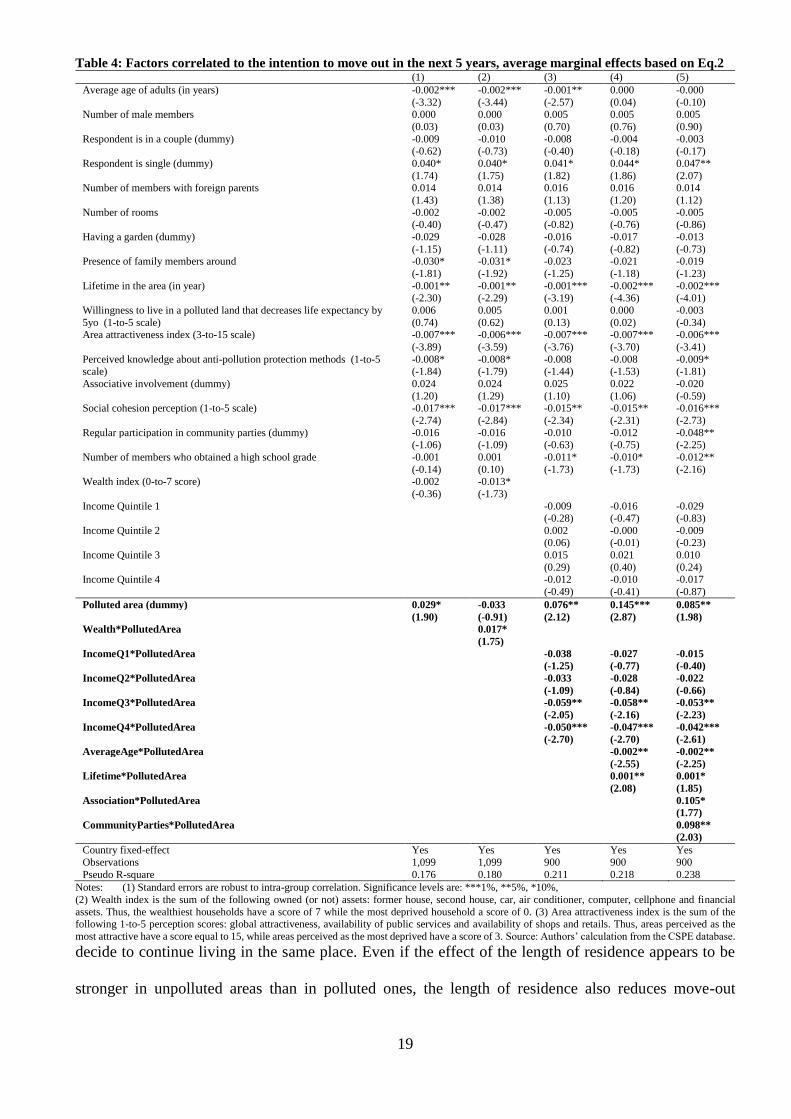
Table 4 shows marginal effects (at the mean) of the intention to move-out in the next 5 years. Several

divergences appear between polluted areas and clean areas. First, compared to control areas, living in

polluted areas increases the intention to move out in the next five years by 3 percentage points (Column

1). Focusing on interaction terms, we observe that both the wealth index and income groups affect the

intention to leave a polluted area. In Column 2, while an extra owned asset reduces the move-out

intention in clean areas by 1.3 percentage point, in polluted areas such an extra asset increases the

probability by 0.4 percentage points. Column 2 also hypothetically indicates that, among extremely

deprived households (with not even one owned asset), living in a polluted area does not affect move-out

intentions. In Column 3, we find that, in polluted areas, households belonging to the third and the fourth

quintiles have lower move-out intentions (around -4 percentage points) compared to households

belonging to the richest income category (Q5). These results emphasize a nonlinear relationship between

household socioeconomic status and the intention to leave a polluted area.

Regarding demographic factors, Column 4 in Table 4 shows that the average age of adult household

members significantly reduces the motivation to move out in households living in polluted areas: 10

extra years in age reduces move-out intentions by 2 percentage points, compared to households living

in cleaner control areas. This result is consistent with the aging theories of mobility and pollution

perception: older individuals are less sensitive to pollution and related risks than younger ones, besides

being less mobile (Lee and Waddell, 2010).5 Community attachment might also explain why people

5 Note that, even if being older reduces the probability of living in polluted areas (as can be seen in Table 2), household

average age can increase the intention to stay. It is likely that older people who chose to stay in polluted areas (before the

survey collection) are the most attached to (or trapped in) the community. Hence, these stayers are likely to remain attached

(or trapped) when we ask for move-out intention.

19

Table 4: Factors correlated to the intention to move out in the next 5 years, average marginal effects based on Eq.2 (1) (2) (3) (4) (5)

Average age of adults (in years) -0.002*** -0.002*** -0.001** 0.000 -0.000 (-3.32) (-3.44) (-2.57) (0.04) (-0.10)

Number of male members 0.000 0.000 0.005 0.005 0.005 (0.03) (0.03) (0.70) (0.76) (0.90)

Respondent is in a couple (dummy) -0.009 -0.010 -0.008 -0.004 -0.003 (-0.62) (-0.73) (-0.40) (-0.18) (-0.17)

Respondent is single (dummy) 0.040* 0.040* 0.041* 0.044* 0.047** (1.74) (1.75) (1.82) (1.86) (2.07) Number of members with foreign parents 0.014 0.014 0.016 0.016 0.014 (1.43) (1.38) (1.13) (1.20) (1.12)

Number of rooms -0.002 -0.002 -0.005 -0.005 -0.005 (-0.40) (-0.47) (-0.82) (-0.76) (-0.86)

Having a garden (dummy) -0.029 -0.028 -0.016 -0.017 -0.013 (-1.15) (-1.11) (-0.74) (-0.82) (-0.73) Presence of family members around -0.030* -0.031* -0.023 -0.021 -0.019 (-1.81) (-1.92) (-1.25) (-1.18) (-1.23)

Lifetime in the area (in year) -0.001** -0.001** -0.001*** -0.002*** -0.002*** (-2.30) (-2.29) (-3.19) (-4.36) (-4.01)

Willingness to live in a polluted land that decreases life expectancy by

5yo (1-to-5 scale)

0.006 0.005 0.001 0.000 -0.003

(0.74) (0.62) (0.13) (0.02) (-0.34) Area attractiveness index (3-to-15 scale) -0.007*** -0.006*** -0.007*** -0.007*** -0.006*** (-3.89) (-3.59) (-3.76) (-3.70) (-3.41)

Perceived knowledge about anti-pollution protection methods (1-to-5 scale)

-0.008* -0.008* -0.008 -0.008 -0.009* (-1.84) (-1.79) (-1.44) (-1.53) (-1.81)

Associative involvement (dummy) 0.024 0.024 0.025 0.022 -0.020 (1.20) (1.29) (1.10) (1.06) (-0.59) Social cohesion perception (1-to-5 scale) -0.017*** -0.017*** -0.015** -0.015** -0.016*** (-2.74) (-2.84) (-2.34) (-2.31) (-2.73)

Regular participation in community parties (dummy) -0.016 -0.016 -0.010 -0.012 -0.048** (-1.06) (-1.09) (-0.63) (-0.75) (-2.25)

Number of members who obtained a high school grade -0.001 0.001 -0.011* -0.010* -0.012** (-0.14) (0.10) (-1.73) (-1.73) (-2.16) Wealth index (0-to-7 score) -0.002 -0.013* (-0.36) (-1.73)

Income Quintile 1 -0.009 -0.016 -0.029 (-0.28) (-0.47) (-0.83)

Income Quintile 2 0.002 -0.000 -0.009 (0.06) (-0.01) (-0.23)

Income Quintile 3 0.015 0.021 0.010 (0.29) (0.40) (0.24) Income Quintile 4 -0.012 -0.010 -0.017 (-0.49) (-0.41) (-0.87)

Polluted area (dummy) 0.029* -0.033 0.076** 0.145*** 0.085** (1.90) (-0.91) (2.12) (2.87) (1.98)

Wealth*PollutedArea 0.017* (1.75)

IncomeQ1*PollutedArea -0.038 -0.027 -0.015 (-1.25) (-0.77) (-0.40)

IncomeQ2*PollutedArea -0.033 -0.028 -0.022 (-1.09) (-0.84) (-0.66)

IncomeQ3*PollutedArea -0.059** -0.058** -0.053** (-2.05) (-2.16) (-2.23)

IncomeQ4*PollutedArea -0.050*** -0.047*** -0.042*** (-2.70) (-2.70) (-2.61)

AverageAge*PollutedArea -0.002** -0.002** (-2.55) (-2.25)

Lifetime*PollutedArea 0.001** 0.001* (2.08) (1.85)

Association*PollutedArea 0.105* (1.77)

CommunityParties*PollutedArea 0.098** (2.03)

Country fixed-effect Yes Yes Yes Yes Yes

Observations 1,099 1,099 900 900 900

Pseudo R-square 0.176 0.180 0.211 0.218 0.238

Notes: (1) Standard errors are robust to intra-group correlation. Significance levels are: ***1%, **5%, *10%,

(2) Wealth index is the sum of the following owned (or not) assets: former house, second house, car, air conditioner, computer, cellphone and financial

assets. Thus, the wealthiest households have a score of 7 while the most deprived household a score of 0. (3) Area attractiveness index is the sum of the following 1-to-5 perception scores: global attractiveness, availability of public services and availability of shops and retails. Thus, areas perceived as the

most attractive have a score equal to 15, while areas perceived as the most deprived have a score of 3. Source: Authors’ calculation from the CSPE database.

decide to continue living in the same place. Even if the effect of the length of residence appears to be

stronger in unpolluted areas than in polluted ones, the length of residence also reduces move-out

20

intentions in polluted areas (Column 4). While living 10 extra years in an unpolluted area reduces move-

out intention by 2 percentage points, in polluted areas, such an increase reduces the move-out intention

by 1 percentage point. Finally, in Column 5, we find a surprising result concerning community

involvement. While participation in community events increases the intention to stay in an unpolluted

area by 4.7 percentage points, the same participation increases the intention to leave a polluted area by

5 percentage points. We observe similar results concerning involvement in associative life. These

findings highlight the presence of a link between community involvement and sensitivity to pollution,

as mentioned by Chanel et al. (2004). Moreover, these results also emphasize the level of social

exclusion of several households who prefer to stay than to move out.

Table B4 in the Appendix shows variables that do not influence move-out intentions differently between

polluted and non-polluted areas. In particular, the attractiveness of an area and the perception of social

cohesion are two of such factors.6 In the same way, household education, marital status and the presence

of a family network affect the intention to move out independently of the residential location. Anywhere,

living close his/her family reduces move-out intentions, whereas being single and educated increases

mobility intention, probably due to better social and professional opportunities elsewhere.

5. DISCUSSION AND CONCLUSION

Our study identified the main determinants that explain why households live and continue to live near

polluted sites in Southwestern Europe. We implemented an IV procedure, which is rarely done in the

connected literature. Globally, our results corroborate the existence of socio-environmental inequalities

in the European context. First, we find that household education reduces the risk of living in polluted

areas. In line with the results from the US literature, environmental disamenities tend to ward off

educated households, whereas environmental amenities attract these population groups (Waltert and

6 The absence of heterogeneous effects according to pollution exposure might be due to the fact that the attractiveness index

and the perception of social cohesion are collinear with residential location. As shown in Table 1, polluted areas are generally

perceived as less attractive and less socially cohesive, which probably affects the probability of living there.

21

Schläpfer, 2010). However, our data distribution suggests that the economic segregation is not as linear

as in the US. The multivariate analysis shows that a lower-middle income class disproportionally lives

in polluted areas in Southwestern Europe. Note that housing size significantly increases the probability

of living in polluted areas for this social group. In addition, there are higher proportions of couples and

young adults who live in polluted areas to benefit from bigger houses. Hence, as pertinently discussed

by Flanquart, Hellequin and Vallet (2013), polluted areas may constitute an acceptable residential

alternative for households with moderate standards of living insofar as such towns provide several

amenities at an affordable price. The overrepresentation of a lower-middle class in larger houses also

matches the assumption of Banzhaf, Ma and Timmins (2019) about the existence of compensations and

benefits for households who accept to live near a polluting industry. Note that these unobserved local

amenities might be a source of endogeneity and could bias the fitted coefficients of socioeconomic

factors. Indeed, when we opt for an endogeneity-corrector approach (the IV strategy), we find a negative

and linear impact of household income and wealth on the risk of living in polluted areas. Finally, we

find a higher proportion of households with members of foreign origin in polluted areas compared to in

control areas. This fact is consistent with a study on France that showed a strong spatial correlation

between towns with a high proportions of immigrant residents and the presence of hazardous sites

(Laurian, 2008).

In terms of move-out intentions, we detect some nonlinearities that might modify the linear vision of

environmental inequalities. In accordance with the mainstream theory, it is particularly the richest

households who plan to move out, probably because of their greater financial capacities and employment

opportunities. Inversely, the most materially deprived households have no move-out intentions given

their limited funding capacities and opportunities. Moreover, among polluted areas, we observe that

people who are not involved in the community life have lower move-out intentions than people who are

involved in community life. To us, these findings suggest the disproportionate presence of socially

excluded groups in polluted areas with no move-out intentions. Our results emphasize the fact that the

general equilibrium theorized by Tiebout (1956) has still not been reached in our sample of polluted

22

areas. However, between the two socioeconomic antipodes, there is a middle class with strong intentions

to remain in polluted areas. As we previously suspected, one can assume that polluted areas in

Southwestern Europe provide some amenities that particularly attract lower-middle classes. Another

interesting result underlines the importance of aging and length of residence as significant determinants

of the intention to remain in polluted areas. This result is in line with the sociological literature. In the

US context, Shriver and Kennedy (2005, p.495) argue that “long-term residents express less concern

over environmental hazards because they are far more attached to their local communities”. In France,

Flanquart, Hellequin and Vallet (2013) observe that populations living alongside hazardous industrial

sites feel a strong community attachment.

The main limitation of this study is linked to the fact that it is measuring local effects. Indeed, strictly

speaking, our results are only valid for our study areas in Southwestern Europe. However, the industrial

heterogeneity of our sample makes our estimate generalizable to a wide spectrum of polluted areas. Of

course, further analyses of the determinants of the socio-environmental segregation in Europe should be

conducted in other contexts (e.g. different case studies and different outcome indicators).

The fact that hazardous polluted areas tend to become economically attractive for lower socioeconomic

groups may be a dramatic public health issue, given that lower social classes tend to have more children.

Additional studies should also assess the health and productivity effects of pollution exposure in addition

to the influence of socioeconomic status on such effects. Finally, our results imply that health policies

or recommendations for averting behaviour should be targeted in particular towards lower-middle class

families, which are the most likely to be attracted by employment and housing opportunities in polluted

areas.

23

REFERENCES

ANGRIST Joshua D., PISCHKE Jörn-Steffen, 2008, Mostly Harmless Econometrics: An Empiricist’s Companion, Princeton University Press,

393 p.

BAILEY Roy E., HATTON Timothy J., INWOOD Kris, 2018, “Atmospheric Pollution, Health, and Height in Late Nineteenth Century Britain”,

The Journal of Economic History, 78(4), pp. 1210–1247.

BANOS-GONZALES Isabel, BAÑOS PAEZ Pedro, 2013, Portmán: De el Portus Magnus del Mediterráneo Occidental a la Bahía Aterrada |

Ediciones de la Universidad de Murcia (Editum), Ediciones de la Universidad de Murcia, Murcia, España, Baños Paez.

BANZHAF H. Spencer, WALSH Randall P., 2008, “Do People Vote with Their Feet? An Empirical Test of Tiebout”, American Economic

Review, 98(3), pp. 843–863.

BANZHAF H. Spencer, WALSH Randall P., 2013, “Segregation and Tiebout sorting: The link between place-based investments and

neighborhood tipping”, Journal of Urban Economics, 74, pp. 83–98.

BANZHAF Spencer, MA Lala, TIMMINS Christopher, 2019, “Environmental Justice: the Economics of Race, Place, and Pollution”, The

Journal of Economic Perspectives: A Journal of the American Economic Association, 33(1), pp. 185–208.

BOWEN William, 2002, “An analytical review of environmental justice research: what do we really know?”, Environmental Management,

29(1), pp. 3–15.

CHANEL Olivier, FAUGERE Elsa, GENIAUX Ghislain, KAST Robert, LUCHINI Stéphane, SCAPECCHI Pascale, 2004, “Valorisation

économique des effets de la pollution atmosphérique: Résultats d’une enquête contextuelle”, Revue économique, 55(1), pp. 65–92.

CONESA Héctor M., SCHULIN Rainer, NOWACK Bernd, 2008, “Mining landscape: A cultural tourist opportunity or an environmental

problem?: The study case of the Cartagena–La Unión Mining District (SE Spain)”, Ecological Economics, 64(4), pp. 690–700.

DE PALMA André, PICARD Nathalie, WADDELL Paul, 2007, “Discrete choice models with capacity constraints: An empirical analysis of

the housing market of the greater Paris region”, Journal of Urban Economics, 62(2), pp. 204–230.

DOHMEN, T. , Falk, A. , Huffman, D. , Sunde, U. , Schupp, J. and Wagner, G. G. (2011), "Individual risk attitudes: measurement,

determinants, and behavioral consequences. Journal of the European Economic Association, 9: 522-550.

DURAND Cécile, SAUTHIER Nicolas, SCHWOEBEL Valérie, 2011, “Évaluation de l’exposition à des sols pollués au plomb, au cadmium et

à l’arsenic en Aveyron”, Rapport de l’Institut de Veille Sanitaire (InVS), France, CIRE/Production scientifique InVS.

FLANQUART Hervé, HELLEQUIN Anne-Peggy, VALLET Pascal, 2013, “Living alongside hazardous factories: risk, choice and necessity”,

Health, Risk & Society, 15(8), pp. 663–680.

GELLER Andrew, ZENICK Harold, 2005, “Aging and the Environment: A Research Framework”, Environmental Health Perspectives,

113(9), pp. 1257–1262.

GRAMAGLIA Christelle, 2015, “Dwelling in polluted places. How issues about risk are raised, avoided or kept silent in two French towns”,

in Peilin Li, Roulleau-Berger Laurence (eds.), Ecological Risks and Disasters - New Experiences in China and Europe, 1 edition,

Abingdon, Oxon ; New York, NY, Routledge.

GUIHARD-COSTA Anne-Marie, INACIO Manuela, VALENTE Sandra, FERREIRA DA SILVA Eduardo, 2012, “Méthode d’étude spatialisée des

effets de la contamination industrielle sur la santé des populations locales, région d’Estarreja (Portugal)”, Sud-Ouest européen. Revue

géographique des Pyrénées et du Sud-Ouest, 33, pp. 69–76.

GUO Jessica Y., BHAT Chandra R., 2007, “Operationalizing the concept of neighborhood: Application to residential location choice

analysis”, Journal of Transport Geography, 15(1), pp. 31–45.

INÁCIO M, NEVES O, PEREIRA V, 2014, “Acumulação de metais pesados em forragens e produtos agrícolas em Podzóis de um local

industrial Português”, Comunicações Geológica, 101, pp. 1019–1022.

JERRETT Michael, BURNETT Richard T, KANAROGLOU Pavlos, EYLES John, FINKELSTEIN Norm, GIOVIS Chris, BROOK Jeffrey R, 2001,

“A GIS–Environmental Justice Analysis of Particulate Air Pollution in Hamilton, Canada”, Environment and Planning A: Economy and

Space, 33(6), pp. 955–973.

LANDRIGAN Philip J., ET AL., “The Lancet Commission on pollution and health”, The Lancet, 391(10119), pp. 462–512.

LAURIAN Lucie, 2008, “Environmental Injustice in France”, Journal of Environmental Planning and Management, 51(1), pp. 55–79.

24

LEE Brian H. Y., WADDELL Paul, 2010, “Residential mobility and location choice: a nested logit model with sampling of alternatives”,

Transportation, 37(4), pp. 587–601.

MARMOT Michael, 2015, “The health gap: the challenge of an unequal world”, The Lancet, 386(10011), pp. 2442–2444.

MILLER Jessica Ty, 2016, “Is urban greening for everyone? Social inclusion and exclusion along the Gowanus Canal”, Urban Forestry &

Urban Greening, 19, pp. 285–294.

MITCHELL Gordon, WALKER Gordon, 2005, “Methodological issues in the assessment of environmental equity and environmental

justice”, in Sustainable Urban Development: The environmental assessment methods, Taylor & Francis, pp. 447–472.

O’NEILL Marie S., JERRETT Michael, KAWACHI Ichiro, LEVY Jonathan I., COHEN Aaron J., GOUVEIA Nelson, WILKINSON Paul,

FLETCHER Tony, CIFUENTES Luis, SCHWARTZ Joel, CONDITIONS Workshop on Air Pollution and Socioeconomic, 2003, “Health, wealth,

and air pollution: advancing theory and methods.”, Environmental Health Perspectives.

PHILLIMORE Peter, BELL Patricia, 2013, “Manufacturing loss: Nostalgia and risk in Ludwigshafen”, Focaal, 2013(67), pp. 107–120.

SCHAEFFER Y., CREMER-SCHULTE D., TARTIU C., TIVADAR M., 2016, “Natural amenity-driven segregation: Evidence from location

choices in French metropolitan areas”, Ecological Economics, 130, pp. 37–52.

SCHIRMER Patrick M., EGGERMOND Michael A. B. van, AXHAUSEN Kay W., 2014, “The role of location in residential location choice

models: a review of literature”, Journal of Transport and Land Use, 7(2), pp. 3–21.

SHRIVER Thomas E., KENNEDY Dennis K., 2005, “Contested Environmental Hazards and Community Conflict Over Relocation*”, Rural

Sociology, 70(4), pp. 491–513.

TIEBOUT Charles M., 1956, “A Pure Theory of Local Expenditures”, Journal of Political Economy, 64(5), pp. 416–424.

VAN DUIJN Mark, ROUWENDAL Jan, 2013, “Cultural heritage and the location choice of Dutch households in a residential sorting model”,

Journal of Economic Geography, 13(3), pp. 473–500.

WALTERT Fabian, SCHLÄPFER Felix, 2010, “Landscape amenities and local development: A review of migration, regional economic and

hedonic pricing studies”, Ecological Economics, 70(2), pp. 141–152.

WOOLDRIDGE Jeffrey M., 2003, “Cluster-Sample Methods in Applied Econometrics”, American Economic Review, 93(2), pp. 133–138.

WOOLDRIDGE Jeffrey M., 2010, Econometric Analysis of Cross Section and Panel Data, Second Edition, Cambridge MA, The MIT Press.

25

APPENDIX A: Additional descriptive statistics about study areas

Table A1: Descriptive statistics of study-areas

Portman/ESG

vs. control Viviez vs.

control Alumbres

vs. control Estarreja

vs. control Attachment to the area

Ratio of area lifetime/age (%) 0.11** 0.08* 0.30*** 0,08***

Intention to move out in the next 5 years (proportion) 0,01 0.13*** 0.10* 0,01

Living here for economic reasons (proportion) 0.19*** 0.12** -0.10* -0,02

Living here for professional reasons (proportion) 0.31*** -0.10* 0.12** 0,20*** Living here for social/family reasons (proportion) 0.10* -0,01 0.15** 0,01

Living here for environmental reasons (proportion) -0.24*** -0.28*** -0.08** -0,09***

Living here for public facilities (proportion) 0.04* -0.07** 0,02 -0,02

Source: Authors’ calculation from the CSPE database.

Figure A1 shows that “social ties” play an important role on residential motivations for all study-areas; as they are more often

mentioned than “professional reasons” and “economic reasons”. Nonetheless, referring to Table A1, “professional reasons”

are particularly mentioned as a motivation for living in Alumbres and Estarreja. Table A1 also shows that residents more

often mention to have chosen to live in Viviez and Portman/ESG for “interesting economic reasons” (e.g. affordable housing

price) compared to residents from non-polluted areas, who more often mention “environmental amenities” as residential

motivation. This result is not surprising given the presence of an active industry supplying various jobs in both areas.

Furthermore, strong community attachment and satisfaction are characteristics that are highlighted in several active industrial

sites in Europe. However, perceived area attractiveness is significantly lower in these active sites (Viviez and Alumbres),

compared to their respective control groups. This might be due to the presence of smokes, smells and noises.

Table A1 also shows stronger intentions to move out for residents from Viviez and Alumbres compared to their respective

control groups. In these two municipalities, “environmental issues” appear as the most mentioned motivation for moving out

(Figure A2). In contrast, “environmental issues” does not appear as a specific move-out issue in Portman/ESG and Estarreja,

compared to their respective counterparts. On the other hand, area attractiveness perceptions in Portman/ESG and Estarreja

do not differ from their respective control areas. This absence of significant gap is not so surprising since, in both areas, there

are close environmental amenities that residents can enjoy despite the presence of pollution (e.g. lagoon, sea, or ocean). In

addition, pollution is not directly visible in Portman/ESG (i.e. mines closed since 1990) and can be relatively far in Estarreja

for people living in other freguesias than Beduido & Veiros (where the chemical complex is located). In the same way, Table

1 does not show significant differences regarding move-out intentions in Portman/ESG and Estarreja, compared to their

respective control group.

26

Figure A1: Main mentioned reason for living in the area

Source: CSPE database, authors’ computation.

Figure A2: Main mentioned reason for move-out intentions in the next 5 years

Source: CSPE database, authors’ computation.

27

APPENDIX B: Additional materials

Table B1: Description of variables used in Eq.1 and Eq.3 Variable name Description

Living in polluted areas (dummy) Takes the value 1 if the household lives in a polluted area (Viviez, Sierra Minera,

Estarreja) and 0 if it lives in a control area (Montbazens, Catargena West, Vagos).

Intention to move out in the next five years Takes the value 1 if the household plans to move out of the community in the next

five years, 0 otherwise.

Number of children (lower than 17yo) Quantity of children in the household.

Number of young adults (18-29yo) Quantity of young adults in the household.

Number of lower-middle age adults (30-44yo) Quantity of lower-middle age adults in the household.

Number of higher middle age adults (45-64yo) Quantity of higher-middle age adults in the household.

Number of old adults (higher than 65yo) Quantity of old adults in the household.

Number of male members Quantity of male members in the household.

Respondent is in a couple (dummy) Takes the value 1 if the respondent is in a couple (married or free union), 0 otherwise.

Respondent is single (dummy) Takes the value 1 if the respondent is single, 0 otherwise.

Number of members with foreign parents Quantity of adult members with foreign parents in the household.

Number of rooms Number of rooms in the housing.

Having a garden (dummy) Takes the value 1 if the housing has a private garden, 0 otherwise.

Presence of family members around (dummy) Takes the value 1 if there are family members living in the same community, 0

otherwise.

Lifetime in the area (in year) Duration of residence in the community in years.

Willingness to live in a polluted land that decreases life expectancy by 5yo (1-to-5 scale)

The scale varies from 1 "a very low willingness to live in a place that may reduce life expectancy by 5yo" to 5 "a very high willingness to take this risk".

Number of members who obtained a high-school grade Number of household members who obtained a high-school diploma

Wealth index (0-to-7 score) Wealth index is the sum of the following owned (or not) assets: former house, second

house, car, air conditioner, computer, cellphone and financial assets. Thus, the wealthiest households have a score of 7 while the most deprived household a score of

0.

ln(monthly total household income) Before being log-transformed, monthly total household incomes are corrected using

purchasing power parities (PPP) based on 2017 US dollars: 0.581 for Portugal, 0.641 for Spain and 0.776 for France.

Respondent's height Height of the respondent in meters

Respondent's parental education Takes the value 1 if at least one parent of the respondent obtained a high-school

diploma, 0 otherwise.

Source: Authors’ computation from the CSPE database.

28

Table B2: Factors correlated to the probability of living in polluted areas, average marginal effects (1) (2) (3) (4)

Number of children (lower than 17yo) -0.006 -0.021 -0.007 -0.020 (-0.19) (-0.75) (-0.26) (-0.75)

Number of young adults (18-29yo) 0.065* 0.054 0.070** 0.055 (1.86) (1.37) (1.97) (1.48)

Number of lower-middle age adults (30-44yo) 0.029 0.030 0.039 0.038 (0.79) (0.60) (1.02) (0.80)

Number of higher middle age adults (45-64yo) -0.024 -0.041 -0.021 -0.039 (-0.85) (-0.89) (-0.81) (-0.92) Number of old adults (higher than 65yo) -0.061** -0.094** -0.051* -0.095** (-2.01) (-2.03) (-1.67) (-2.11)

Number of male members -0.028 -0.008 -0.031 -0.012 (-1.04) (-0.23) (-1.12) (-0.35)

Respondent is in a couple (dummy) 0.040 0.087** 0.054** 0.107*** (1.53) (2.57) (2.16) (2.91) Respondent is single (dummy) 0.072 0.127** 0.071 0.107* (1.38) (2.36) (1.40) (1.93)

Number of members with foreign parents 0.093*** 0.085*** 0.091*** 0.082*** (3.53) (2.94) (3.58) (2.82)

Number of rooms 0.055*** 0.056*** 0.086*** 0.129*** (3.94) (3.60) (3.87) (3.60)

Having a garden (dummy) -0.181*** -0.165** -0.186*** -0.156** (-2.96) (-2.46) (-2.95) (-2.25)

Presence of family members around (dummy) 0.154** 0.176*** 0.156** 0.187*** (2.04) (2.58) (2.11) (2.61)

Lifetime in the area (in year) 0.004*** 0.005*** 0.004*** 0.004*** (5.17) (5.52) (5.23) (5.19) Willingness to live in a polluted land that decreases life expectancy by 5yo

(1-to-5 scale)

0.101** 0.096** 0.103** 0.099**

(2.36) (2.22) (2.40) (2.32)

Number of members who obtained a high school grade -0.076*** -0.061* -0.086*** -0.063* (-2.58) (-1.82) (-3.02) (-1.87)

Wealth index (0-to-7 score) 0.125*** (3.45)

Square of wealth index -0.017*** (-2.83)

ln(monthly total household income) 1.140** (2.08)

Square of ln(income) -0.075**

(-2.05)

Wealth - Tercile 1 0.342*** (2.66)

Wealth - Tercile 2 0.252**

(2.24)

RoomNumber*WealthT1 -0.055**

(-2.49)

RoomNumber*WealthT2 -0.016

(-0.88)

Income - Quintile 1 0.618*** (3.54)

Income - Quintile 2 0.462** (2.47) Income - Quintile 3 0.363** (2.19)

Income - Quintile 4 0.306 (1.44)

RoomNumber*IncomeQ1 -0.130*** (-3.50)

RoomNumber*IncomeQ2 -0.084** (-2.31)

RoomNumber*IncomeQ3 -0.054* (-1.69)

RoomNumber*IncomeQ4 -0.052

(-1.39)

Country fixed effects Yes Yes Yes Yes

Observations 1,144 939 1,144 939

Pseudo R-square 0.119 0.126 0.127 0.137 Observed probability 0.576 0.573 0.576 0.573

Predicted probability 0.586 0.583 0.588 0.585

Notes: (1) Standard errors are robust to intra-group correlation. Significance levels are: ***1%, **5%, *10%,

(2) Wealth index is the sum of the following owned (or not) assets: former house, second house, car, air conditioner, computer, cellphone and financial assets. Thus, the wealthiest households have a score of 7 while the most deprived household a score of 0.

(3) Before being log-transformed, household incomes are corrected using purchasing power parities (PPP) based on 2017 US dollars: 0.581 for

Portugal, 0.641 for Spain and 0.776 for France. (4) Potential endogenous regressors are in bold between sidebars.

Source: Authors’ calculation from the CSPE database.

29

Table B2 lists average marginal effects at the mean point. Household socioeconomic factors are strong predictors of

residential location. For example, column 1 shows a U-inverted relationship between wealth index and the probability of

living in polluted areas (the turning point being around 3-4 owned assets). In the same way, Column 2 indicates a similar U-

inverted relationship when logged household income (adjusted in $PPP) is used instead of wealth index (the turning point

being around 1918 $PPP, i.e. 1,113 euros in Portugal, 1,230 euros in Spain, and 1,489 euros in France). Households with

lower-middle wealth and income have the highest probability of living in polluted areas, in line with results in Figure 3.7

Interestingly, housing size is a significant predictor of the probability of living in polluted areas, especially for young families

with moderate wealth and incomes. For households belonging to the first wealth tercile, an extra room per housing unit

increases the probability of living in polluted areas by 3.2 percentage points (Column 3).8 Using interaction terms (Column

4), we find that, for households belonging to the first, second and third income quintiles, an extra room increases this

probability by 0.3, 4.3 and 7.4 percentage points, respectively. It is worth noting that, even if households with lower

socioeconomic status can live in larger houses at affordable price in polluted areas, they are significantly less likely to enjoy

having a private garden (a reduction of around 17-19 percentage points), perhaps because of heavy contamination of the soil.

Apart from socioeconomic patterns, other factors may explain why individuals live in polluted areas. For instance, community

attachment seems to increase the risk of living near polluted sites. Indeed, the presence of a family network increases the risk

by 15-18 percentage points, while 10 extra years of living in the area increases it by 4-5 percentage points. Moreover, for all

model specifications, families of foreign origin and households with a low level of education have higher risks of living in

polluted areas. For instance, in Column 1, one extra member with parents of foreign origin increases the probability of living

in a polluted area by nine percentage points.

Demographic factors also produce interesting results. In terms of marital status, single individuals and couples have a higher

probability of living in polluted areas compared to individuals who have suffered from marital upheavals (divorce, separation

or widowhood), except in Column 1 when wealth is controlled for (i.e. potential collinearity between wealth and marital

status). The proportion of old adults in the household reduces the probability of living in polluted areas. This

underrepresentation of the elderly in polluted areas is consistent with the literature showing that the retirees are significantly

attracted by environmental factors (van Duijn and Rouwendal, 2013). Moreover, frail elderly people tend to be more

threatened by mortality risks due to daily pollution exposure than younger individuals (Geller and Zenick, 2005).

Finally, as expected, environmental health risk aversion is negatively correlated with the probability of living in polluted

areas. In other words, people who live near mining- and industrial wastes tend to be more risk-takers concerning the health

effects of daily exposure to pollution.9

Table B3: First-step estimates in IV model, linear regression of household socioeconomic status on instruments and

control variables

Number of

educated

members

Number of

educated

members

Wealth

index

Wealth

index ln(income) ln(income)

Height of the respondent (in meters) 1.252*** 1.157*** 1.611*** 1.490*** 0.943*** 0.866***

7 We regress wealth index and household incomes in independent specifications to avoid multi-collinearity problems.

8 An alternative model specification adding interaction terms between age groups proportions and housing size shows that

housing size particularly increases the probability of living in polluted areas for the 30-45 age group (not shown).

30

(4.09) (3.64) (3.57) (3.30) (4.54) (4.15)

Parental education of the respondent (at least a high-

school diploma)

0.433*** 0.333*** 0.266***

(5.13) (3.11) (5.21)

Number of children (lower than 17yo) 0.006 -0.011 0.055 0.029 0.036 0.027 (0.07) (-0.15) (1.10) (0.57) (0.90) (0.61) Number of young adults (18-29yo) 0.607*** 0.538*** 0.248*** 0.193*** 0.267*** 0.228*** (9.86) (7.58) (3.74) (3.09) (5.50) (4.58)

Number of lower-middle age adults (30-44yo) 0.498*** 0.440*** 0.349*** 0.310*** 0.367*** 0.350*** (7.14) (7.88) (4.33) (3.72) (10.29) (9.59)

Number of higher middle age adults (45-64yo) 0.351*** 0.343*** 0.373*** 0.365*** 0.268*** 0.275*** (7.50) (9.30) (4.94) (4.47) (7.97) (8.33) Number of old adults (higher than 65yo) 0.131** 0.126** -0.044 -0.041 0.149*** 0.170*** (2.13) (2.36) (-0.42) (-0.41) (4.83) (5.21) Number of male members -0.082 -0.061 -0.028 -0.017 -0.040 -0.031 (-1.50) (-0.99) (-0.47) (-0.24) (-1.49) (-1.04)

Respondent is in a couple (dummy) 0.070 0.042 0.696*** 0.717*** 0.252*** 0.237*** (0.86) (0.53) (7.67) (7.89) (6.79) (7.78)

Respondent is single (dummy) -0.076 -0.163 0.324*** 0.346*** 0.089 0.059 (-0.75) (-1.50) (3.05) (3.19) (1.23) (1.00) Number of rooms 0.052*** 0.047*** 0.220*** 0.235*** 0.076*** 0.071*** (3.81) (3.18) (7.83) (9.60) (5.64) (5.19)

Constant -2.536*** -2.347*** -0.787 -0.703 4.961*** 5.085***

(-5.19) (-4.45) (-1.03) (-0.91) (13.73) (13.71)

Country fixed effects Yes Yes Yes Yes Yes Yes

Observations 1,147 1,098 1,147 1,098 943 911

R-square 0.302 0.329 0.340 0.353 0.436 0.464

Notes: (1) Standard errors are robust to intra-group correlation. Significance levels are: ***1%, **5%, *10%, (2) Wealth index is the sum of the following owned (or not) assets: former house, second house, car, air conditioner, computer, cellphone and

financial assets. Thus, the wealthiest households have a score of 7 while the most deprived household a score of 0. Incomes are in US$ PPA.

Source: Authors’ calculation from the CSPE database.

31

Table B4: Reduced-form regression of the dependent variable on the instruments, marginal effects Prob(LivingPollutedAreas)

Height of the respondent (in meters) -0.548*** (-3.02)

Parental education of the respondent (at least a high-school level) -0.075*

(-1.80)

Number of children (lower than 17yo) -0.003 (-0.10)

Number of young adults (18-29yo) 0.019 (0.56)

Number of lower-middle age adults (30-44yo) -0.003 (-0.07)

Number of higher middle age adults (45-64yo) -0.061* (-1.84)

Number of old adults (higher than 65yo) -0.037 (-1.04)

Number of male members -0.018 (-0.59)

Respondent is in a couple (dummy) 0.049 (1.08)

Respondent is single (dummy) 0.085 (1.64)

Number of rooms 0.045*** (4.51)

Country fixed effects Yes

Observations 1,098

R-square 0.0295

Source: Authors’ calculation from the CSPE database.

32

Table B5: Factors of interest NOT correlated to the intention to move out of polluted areas in the next 5 years, average

marginal effects based on Eq.2 Prob(move-out)

Average age of adults (in years) -0.002*** (-3.59) Number of male members -0.001 (-0.09)

Respondent is in a couple (dummy) -0.004 (-0.26)

Respondent is single (dummy) 0.040* (1.82) Number of members with foreign parents 0.015 (1.39) Number of rooms -0.003 (-0.31)

Having a garden (dummy) 0.002 (0.06)

Presence of family members around -0.052* (-1.77) Lifetime in the area (in year) -0.001** (-2.27)

Willingness to live in a polluted land that decreases life expectancy by 5yo (1-to-5 scale) 0.012 (0.59)

Area attractiveness index (3-to-15 scale) -0.006** (-1.97)

Perceived knowledge about anti-pollution protection methods (1-to-5 scale) -0.002

(-0.43)

Associative involvement (dummy) 0.021 (1.12)

Social cohesion perception (1-to-5 scale) -0.010 (-0.75) Regular participation in community parties (dummy) -0.012 (-0.85)

Number of members who obtained a high school grade -0.007 (-0.82)

Wealth index (0-to-7 score) -0.003 (-0.46)

Polluted area (dummy) 0.107 (1.31)

HighSchool*PollutedArea 0.011 (1.03)

HousingSize*PollutedArea 0.001 (0.13)

Garden*PollutedArea -0.044 (-1.28)

RiskTaker*PollutedArea -0.008 (-0.40)

FamilyNetwork* PollutedArea 0.031 (1.09)

Attractiveness*PollutedArea -0.002 (-0.71)

SocialCohesion* PollutedArea -0.011 (-0.77)

ProtectionMethods*PollutedArea -0.008

(-1.05)

Country fixed-effect Yes Observations 1,099

Pseudo R-square 0.184

Notes: (1) Standard errors are robust to intra-group correlation. Significance levels are: ***1%, **5%, *10%, (2) Wealth index is the sum of the following owned (or not) assets: former house, second house, car, air conditioner, computer, cellphone and

financial assets. Thus, the wealthiest households have a score of 7 while the most deprived household a score of 0.

(3) Area attractiveness index is the sum of the following 1-to-5 perception scores: global attractiveness, availability of public services and availability of shops and retails. Thus, areas perceived as the most attractive have a score equal to 15, while areas perceived as the most deprived

have a score of 3.

Source: Authors’ calculation from the CSPE database.

CEE-M Working Papers1 - 2019

WP 2019 - 01 Adrien Nguyen-Huu. & Antonin Pottier

«Hicksian Traverse Revisited: Conditions for the Energy Transition» WP 2019 - 02 Oumar Mbodji, Adrien Nguyen-Huu & Traian A. Pirvu

«Optimal Sharing Rule for a Household with a Portfolio Management Problem»

WP 2019 - 03 Tristan Cotty, Tristan, Elodie Maitre d’Hotel &Julie Subervie

«Inventory credit to enhance food security in Africa» WP 2019 - 04 Raphael Soubeyran

«Incentives, Pro-social Preferences and Discrimination» WP 2019 - 05 Adrien Fabre, Mouez Fodhaz & Francesco Ricci

«Optimal Timing of Energy Production» WP 2019 - 06 Claude Bismut & Ismaël Rmajo

«A world of low interest rates» WP 2019 – 07 Gabriela Demarchi, Julie Subervie, Fernando Palha Leite & Jean-Paul

Laclau « Farmers’ preferences for water-saving strategies in brazilian eucalypt

plantation » WP 2019 - 08 Arnaud Tognetti, David Doat, Dimitri Dubois & Rustam Romaniuc

« Does the presence of a physically disabled erson in the group increase cooperation? An experimental test of the empathyaltruism hypothesis »

WP 2019 – 09 Isabelle Tritsch, Gwenole Le Velly, Benoit Mertens, Patrick, Meyfroidt,

Christophe Sannier, Jean-Sylvestre Makak & Kenneth Houngbedji « Do Forest-Management Plans and FSC Certification Reduce deforestation in the Congo Basin? »

WP 2019 - 10 Jean-Michel Salles

« Valuing the loss and damage from climate change: a review of some current issues »

WP 2019 - 11 Can Askan Mavi « Can harmful events be another source of environmental traps? » WP 2019 - 12 Daniel Serra « Neuroeconomics and Modern Neuroscience »

1 CEE-M Working Papers / Contact : laurent.garnier@inra.fr

RePEc https://ideas.repec.org/s/hal/wpceem.html HAL https://halshs.archives-ouvertes.fr/CEE-M-WP/

WP 2019 - 13 Daniel Serra « La neuroeconomie en question : debats et controversies » WP 2019 - 14 Claire Richert, Katrin Erdlenbruch�& Frédéric Grelot

« The impact of �flood management policies individual adaptation actions: insights from a French case study »

WP 2019 - 15 Margaux Lapierre, Alexandre Sauquet & Julie Subervie

« Improving Farm Environmental Performance through Technical Assistance: Empirical Evidence on Pesticide Use»

WP 2019 - 16 Pierre Levasseur, Katrin Erdlenbruch & Christelle Gramaglia

« Why do people continue to live near polluted sites? Empirical evidence from Southwestern Europe