why do most countries set high tax rates on capital? do most countries set high tax rates on ......
TRANSCRIPT
Why Do Most Countries Set High Tax Rates on Capital??
Nicolas MarceauUniversite du Quebec a Montreal and CIRPEE
Steeve MongrainSimon Fraser University, RIIM, and CIRPEE
John D. WilsonMichigan State University
June 2007
Marceau: [email protected]
Mongrain: [email protected]
Wilson: [email protected]
? We have benefited from our discussions with Nicolas Boccard, Claude Fluet, Richard Harris, Gordon Myers,
Frederic Rychen, Nicolas Sahuguet, and Michael Smart. We also thank seminar participants at HEC-Montreal,
Queen’s University, Simon Fraser University, Universite de Cergy-Pontoise, Universite de Lille 3, University
of Oregon, Canadian Public Economics Group 2004, International Institute of Public Finance 2004, Journees
du CIRPEE 2005, and Les Journees Louis-Andre Gerard-Varet 2004 for their comments. Financial support
from FQRSC, RIIM, and SSHRCC is gratefully acknowledged.

Abstract: We consider tax competition in a world with tax bases exhibiting different degrees
of mobility, modeled as mobile and immobile capital. An agreement among countries not to
give preferential treatment to mobile capital results in an equilibrium where mobile capital is
nevertheless taxed relatively lightly. In particular, one or two of the smallest countries, mea-
sured by their stocks of immobile capital, choose relatively low tax rates, thereby attracting
mobile capital away from the other countries, which are then left to set revenue maximizing
taxes on their immobile capital. This conclusion holds regardless of whether countries choose
their tax policies sequentially or simultaneously. In contrast, unrestricted competition for
mobile capital results in the preferential treatment of mobile capital by all countries, without
cross-country differences in the taxation of mobile capital. Nevertheless our main result is that
the non-preferential regime generates larger global tax revenue, despite the sizable revenue
loss from the emergence of low-tax countries. By extending the analysis to include cross-
country differences in productivities, we are able to resurrect a case for preferential regimes,
but only if the productivity differences are sufficiently large.
Keywords: Tax Competition, Capital Mobility
JEL Classification: F21, H87

1. Introduction
A theme running through the tax competition literature is that jurisdictions face incentives
to compete for mobile capital by reducing their tax rates. As a result, tax competition leads
to inefficiently low tax rates and public good provision when governments are welfarist, but
may constrain the excessive size of government that act as Leviathans.1 One might question
the tax-reducing effects of tax competition when examining the effective average capital tax
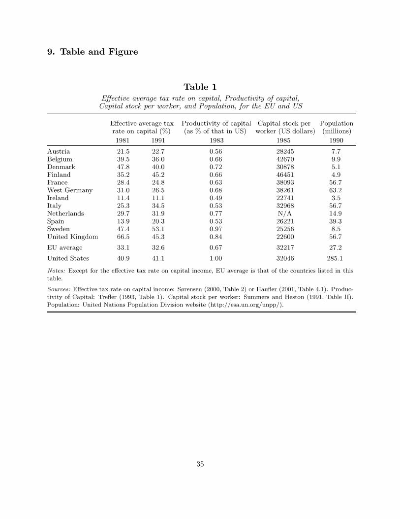
rates in the European Union for the year 1991, which we report in Table 1.2 Indeed, note that
most of the countries are distributed around an average of 32% – with some variance, possibly
explained by differences in preferences for publicly provided goods – while on the other hand,
a considerably lower tax rate of only 11% is in effect in Ireland.3 An interpretation of such
facts is that Ireland was undercutting the other countries, while the rest seemed to act as if
it was business as usual. Intuitively, if a country has a comparative advantage at lowering its
tax rate to attract mobile capital, it will specialize in this activity. However, the rest of the
countries will not attempt to attract mobile capital, and will instead focus on their immobile
base to finance their expenditures.
These observations raise questions about the extent to which countries actively compete for
capital in an increasingly integrated world economy. Despite increasing capital mobility, Hines
(2005) presents evidence showing that in a group of 68 countries, corporate tax collections
did not decline as a percentage of GDP between 1982 and 1999.4 He attributes this finding
to a switch in tax burdens from mobile capital to immobile capital, along with an expansion
1 See Wilson (1999) for a review of the tax competition literature, and Wilson (2005) for a recentanalysis of competition with self-interested government officials.
2 Effective average tax rates measure total taxes paid as a fraction of the relevant tax base. In thecase of the average capital tax rates reported in Table 1, they include corporate tax collectionas well as personal taxes on capital income. See Sørensen (2000) or Haufler (2001).
3 Similar patterns can be observed in the 1981 tax rates, except for the fact that Spain and Irelandboth have very low tax rates.
4 Note however that for the US, corporate tax collections seem to have declined rapidly between1960 and 1982. On this, see Auerbach (2005).
1

of domestic tax bases. Such a switch could be brought about by the type of specialization
described above, but it could also signal the use of preferential tax regimes by individual
countries, whereby mobile capital is taxed more lightly than immobile capital.
This view that the revenue-reducing effects of tax competition might be mitigated by the
differential treatment of mobile and immobile tax bases is not universally shared by economists
and policymakers. Recently, the OECD became interested in what it calls “harmful tax
practices”. In OECD (1998), in the context of countries engaged in the taxation of mobile
tax bases, two sorts of country behaviour are viewed as harmful: (a) To impose no or very low
taxes on some bases; and (b) To have some preferential features in the tax system that allow
part of a given base to escape taxation. For the second sort of behaviour, the preferential tax
regimes often consist in the foreign-owned portion of a tax base being taxed at a lower rate
than the domestic-owned portion, a behaviour which is also labeled “discrimination”.5
The theoretical literature on preferential versus non-preferential tax regimes is inconclusive.
Janeba and Peters (1999) show that the elimination of preferential regimes leads to higher
total levels of tax revenue. On the other hand, Keen (2001) reaches the opposite conclusion.
They both analyze simultaneous-move Nash games in tax rates, but their models contain
important differences. Janeba and Peters consider two countries that differ in their supplies
of an immobile “domestic tax base,” whereas a second base is infinitely elastic with respect to
differences in tax rates: it locates in the lowest-tax country. In contrast, Keen assumes that
both countries are completely identical and have access to two tax bases that are partially-
mobile to different degrees. Wilson (2005) observes, however, that if one of the tax bases
in Keen’s paper were made infinitely elastic, as in Janeba and Peters, then a symmetric
5 Note that some countries – e.g. Canada and the US – have signed mutually advantageous taxtreaties which would be jeopardized if one or the other actor were to start discriminating. Andthe prohibition of the asymmetric treatment of foreign and domestic firms has been included intreaties in the EU and the OECD. Both the OECD and the EU are active in trying to reducethe extent of discrimination among their members. On this, see OECD (1998).
2
equilibrium in pure strategies would not exist.6
In an effort to sort out these competing views, we first develop a model in which countries
are first constrained to use a non-preferential regime which imposes the same tax rate on
immobile and perfectly mobile capital. This leads to an equilibrium in which there is never-
theless differential taxation of mobile and immobile capital, not within individual countries,
but rather because mobile capital locates in countries with low tax rates on all capital. Con-
sistent with the EU case described above, a small number of countries act as “tax havens,”
setting their tax rates at relatively low levels and thereby attracting large amounts of the
mobile base, leaving the majority of countries to impose higher tax rates on their remaining
(immobile) capital. This result suggests that another OECD initiative — to limit tax havens
— complements their guidelines for limiting preferential treatment of mobile capital.7
When countries are allowed to individually levy different tax rates on immobile and mobile
capital, tax havens do not emerge in our model, but tax competition for mobile capital
intensifies, causing a large revenue loss in the form of lower tax rates on mobile capital.
This comparison raises the intriguing question of whether it is preferable to bring about the
differential treatment of mobile and immobile capital through the operation of tax havens in a
non-preferential regime, or through preferential treatment without tax havens. We conclude
that tax competition in the non-preferential regime leads to a lower aggregate loss in tax
revenue, compared with tax competition in the preferential regime. Note, however, that
6 Janeba and Smart (2003) generalize both the Janeba-Peters and Keen results to more generalsettings. But they also must restrict the relevant elasticities to ensure the existence of equilibriain pure strategies. Wilson (2005) analyzes mixed strategies, but he considers only symmetricequilibria for identical countries, whereas the focus of the current paper is on the emergence oflow-tax countries (tax havens).
7 In 2000 the OECD published a list of 35 countries called “non-cooperating tax havens,” givingthem a year to enact fundamental reform of their tax systems and broaden the exchange ofinformation with tax authorities or face economic sanctions. By 2005 almost all of the blacklistedtax havens had signed the OECD’s Memorandum of Understanding agreeing to transparencyand exchange of information.
3

revenue would be higher in the non-preferential regime if there were no tax havens. 8
We demonstrate that the superiority of the non-preferential regime in terms of tax revenue
does not require assumptions about whether countries choose their tax rates simultaneously
or sequentially. Thus, we do not need to justify a particular order of moves, though a case
might be made for sequential-move games based on institutional constraints on the ability of
countries to adjust tax rates quickly. Our assumption of a highly-mobile tax base precludes
the existence of a simultaneous-move pure strategy equilibrium in the non-preferential-regime
case, but we are still able to make comparisons by allowing countries to use mixed strategies.
In addition, we find that all countries obtain at least the same expected tax revenue under
the equilibrium for the sequential-move game as they do when the simultaneous-move game is
played, with expected tax revenue higher for some countries when non-preferential treatment
is required. As a result, we should not be surprised not to observe mixed strategies being
played in practice.
Our analysis of non-preferential regimes also yields the finding that those countries that
emerge as ”tax havens” are the smallest ones. A similar result is found in the literature
on asymmetric tax competition.9 The intuition is that smaller countries face a more elastic
tax base, giving them incentives to set lower tax rates. In these papers, population is the
measure used to describe a small country. But in Table 1, the correlation between the size –
population – of a country and its tax rate is not clear. For example, some large countries like
Germany and France have below average tax rates. In 1991, it is clearly the smallest country
on the list – Ireland – that has the lowest tax rate. However, for 1981, both Ireland and
8 The term “tax haven” is being applied here to countries that offer low tax rates on real capitalinvestments, rather than countries that facilitate income-shifting for the purpose of reducingtaxable income in high-tax countries, independently of the location of physical investments.Slemrod and Wilson (2006) analyze tax competition in the latter setting and conclude that taxhavens worsen the tax competition problem, resulting in lower levels of welfare.
9 On asymmetric tax competition, see Bucovetsky (1991), Kanbur and Keen (1993), and Wilson(1991).
4

Spain – which has an above average population size – are neck to neck for the lowest tax rate.
Note further that if small countries have low tax rates, then they should become importers of
capital, giving them relatively high capital/labor ratios, all else equal. But Table 1 also fails
to support this prediction. For example, Ireland and Spain have capital/labour ratios below
the EU average. In fact, this small set of European data reveals that the 1991 capital taxes
and population have a negative correlation factor of -0.108. To summarize, the predictions
of the asymmetric tax competition literature do not appear to be realized in the real world
equilibrium. Hines (2005) also comments on this lack of correlation between country size and
tax rates, noting that it had largely disappeared by 1999.
In this paper, we introduce a different measure of country size. Countries are allowed
to differ in their endowments of “immobile capital,” and it is the country with the lowest
endowment that will choose the lowest tax rate. The intuition is simply that such a country
has the least to lose by lowering its tax rate. Our framework therefore suggests that countries
with low capital/labour ratios are more likely to set very low tax rates to attract mobile
capital. Table 1 provides some evidence on this issue. While some high capital/labour ratio
countries – e.g. Sweden and UK – do set high tax rates, it remains that the very low tax rates
are found in countries with low capital/labour ratio – e.g. Ireland and Spain. The correlation
between the 1991 tax rates and the capital/labor ratio is small but positive (at 0.169).
We later extend the analysis to allow countries to possess different productivities. For non-
preferential regimes, an intriguing result is that for countries of equal size, it may be the one
with the lowest productivity that will set the lowest tax rate. The same intuition applies:
a country with a low productivity generates less tax revenues from its immobile tax base,
and can consequently be more aggressive. This implies that mobile capital may have the
tendency to inefficiently locate in less productive countries. Depending on the size of these
productivity differences, this result could counteract the superior revenue-raising capabilities
of non-preferential regimes. Table 1 also reports some data on the productivity of capital.
5

Our explanation could account for the case of Ireland — low productivity and low tax rates,
and could also help explain the low tax rate chosen by Spain in 1981. Our explanation is
also supported by the fact that as Spain’s productivity rose in the eighties, so did its tax
rate.10 Note that overall, the correlation between the 1981 tax rates and the 1983 capital
productivity is strongly positive at 0.848.
The plan of this paper is as follows. In the next section, we first describe the basic model, with
countries of different sizes and no productivity differences. For the case where all countries
choose their tax rates simultaneously, we show in Section 3 that there exists a simultaneous-
move Nash equilibrium in which the smallest two countries play mixed strategies, with their
tax rates undercutting the tax rates chosen by the remaining countries. Thus, these two
countries obtain all of the mobile capital in equilibrium. We also analyze the case where all
countries are identical, finding that there also exist equilibria where more than two countries
play mixed strategies and obtain the mobile capital. In Section 4, we introduce a sequential-
move game in which each country chooses its tax rate in a specific, randomly determined,
order. As noted above, this game produces only a single tax haven and leads to higher global
tax revenue than the simultaneous-move game. Section 5 contains the comparison between
preferential and non-preferential regimes, along with extending the analysis to the case where
countries possess different productivities. Section 6 concludes.
2. The Basic Model
Consider a world in which there are J ≥ 2 countries indexed by j, j = 1, ..., J . In each country,
a representative citizen owns a constant return to scale technology F (K) = γK, with γ > 0,
that transforms capital into output. Capital owners can be local or mobile. In country j,
there are Nj local capital owners, and they can only invest in their country. The world is also
10 Data on total factor productivity for Spain in the eighties can be found in Aiyar and Dalgaard(2001).
6

populated by M mobile capital owners who can invest in any of the J countries.11 Capital
owners, whether local or mobile, will also choose the size of their investment. Denote by I the
investment choice made by all capital owners. If the Nj local capital owners and the M mobile
capital owners invest I units of capital in j, then output in j is F (NjI +MI) = γ(Nj +M)I.
Thus, all capital is perfectly substitutable in production.
Capital bears a per unit tax of tj in country j. Given the constant return to scale technology in
each country, the net return of capital in country j is then simply (γ−tj). The owners of local
capital can adjust to taxation by increasing or decreasing the size of their capital investment
I. As for the owners of mobile capital, they too can adjust the size of their investment, but
they can also adjust by choosing to invest in the country which offers them the highest net
return.
The decision of a mobile capital owner as to where to invest is a simple one. The net return
they obtain for each unit they invest in country j is (γ − tj), j = 1, ..., J . Obviously, they will
choose to invest in the country with the lowest tax rate, i.e. in country g if min{tj}Jj=1 = tg.
For now, we assume that if S countries have chosen the same lowest tax rate, then all capital
owners invest in a country belonging to this set with probability 1/S.12 Thus, all of mobile
capital always ends up in a single country (i.e. capital investment is bang-bang), and the
other countries obtain nothing.13
The general timing of events in this world is as follows. First, countries choose their tax rates
11 Note that M (along with some other measure defined below) can be viewed as one of severaldimensions of the size of investment.
12 For heuristic reasons, we introduce a different breaking rule when the game is sequential.
13 Our results would obtain even if the assumption that all investments are bunched were relaxed.In our framework, we simply assume that the marginal product of capital is constant in a givencountry. Departing from the standard assumption of a declining marginal product of capital isfrequent in the literature and simplifies our analysis. For papers which investigate the case inwhich capital tends to agglomerate because of an increasing marginal product, see Baldwin andKrugman (2004), Boadway, Cuff and Marceau (2004), Kind, Knarvik and Schjelderup (2000).
7
tj, j = 1, ..., J . Note that the tax rate in a given country applies to the two types of capital;
discriminating is simply assumed to be impossible. Second, the owners of mobile capital select
the country in which they will invest. Third and finally, owners of local and mobile capital
choose the size of their investment. We will in turn consider the case where the countries
play simultaneously, and that in which they play sequentially, so the first stage will later be
decomposed into two sub-stages.
Owners of capital located in i (be it local or mobile) adjust the size of their investment to
maximize their net consumption, which is simply the total return on their investment minus
the cost of investment, which is given by c(I), with c′ > 0 and c′′ > 0. Thus, for capital
owners in j, the optimal size of their investment is:
I(tj) = arg maxI
(γ − tj)I − c(I)
Of course, given the owners of mobile capital have decided to invest in j, the problem faced by
the owners of local capital and those of mobile capital is identical. The first order condition
characterizing the investment decision I(tj) is (γ− tj)− c′(I) = 0. Using it, we easily get that
I ′(tj) = −1/c′′(I) < 0.
Given our focus on the revenue effects of tax competition, it is natural to assume that tax
revenue plays a prominent role in government objectives. For simplicity, we assume that
governments maximize revenue, but we later argue that our analysis holds more generally.14
Let mj be an indicator function which takes a value of 1 if all mobile capital owners invest in
country j, and a value of 0 if they have opted for any other country. Thus, tax revenue for
country j are tj[Nj + Mmj ]I(tj). We denote by W j(t, m) the tax revenue in country j when
it has chosen tax rate t and when the indicator variable takes a value of m. Thus, we have:
14 Note that Janeba and Peters (1999), a paper which is close to ours, considers a world in whichgovernments maximize tax revenues. Edwards and Keen (1996), Kanbur and Keen (1993), Keen(2001), or Wilson (2005) make this same assumption.
8

W j(t, 1) = t[Nj + M ]I(t)
W j(t, 0) = tNjI(t)
For future use, denote by t the tax rate which maximizes W j(t, 0) and W j(t, 1).15 Also note
that both W j(t, 0) = W j(t, 1) = 0 at both t = 0 and some t > t. Finally, we define tj < t
as the tax rate solving W j(tj , 1) = W j(t, 0), i.e. tjI(tj)(M + Nj) = tI(t)Nj . This implies
that each country has a specific tj, that tj = 0 when Nj = 0, and that tj increases when Nj
increases. The payoff functions of a given country are represented in Figure 1.
— FIGURE 1 —
Irrespective of where mobile capital ends up locating, global tax revenue, summed across all
countries, is maximized when tax rates are set at tj = t ∀ j, j = 1, ..., J . Thus, because
all locations are equivalent, the sole inefficiency that can arise, and that on which we first
want to focus, is the under-taxation of capital. In Section 5, we allow the productivity of
investment to vary between countries, thereby making some locations better than others, and
introducing the possibility of an inefficient location.
3. Equilibrium of the Simultaneous Move Game
Consider first two special cases that are interesting and useful to understand.
In the first special case, there are no mobile capital owners, so M = 0. In this case, because
there is no mobile factor over which the countries can fight, global tax revenue is maximized.
In particular, governments set tj = t ∀ j, j = 1, ..., J , and each country obtains revenue
W j(t, 0), j = 1, ..., J .
15 Note that given the present formulation of the model, t maximizes both W j(t, 0) and W j(t, 1).
9
As a second special case, suppose there is some mobile capital but no local capital, so Nj = 0,
j = 1..., J . In such a case, competition will drive tax rates to zero, and no revenue will be
generated in equilibrium. This equilibrium is obviously the worse possible outcome in this
world.
Note that the allocation in these two special cases does not depend on the timing of the game
or on the relative size of the countries. Obviously, in the absence of mobile capital owners, the
timing is irrelevant since the decisions made by the countries are essentially independent. As
for the case where there is only mobile capital, the equilibrium features zero revenue regardless
of the timing.
The general case we now want to consider is one in which there are J countries differing in their
number of local capital owners. Without loss of generality, suppose that N1 ≥ N2 ≥ ... ≥ NJ .
Three preliminary results turn out to be useful. The proofs of all lemmas and propositions
are in the Appendix.
Lemma 1: Country i never chooses a strategy ti > t.
Note that t is independent of the relative size of Ni and M , so that the same upper bound
on strategies applies to the countries whether they are identical or different. Lemma 1 simply
states that it does not pay to play a tax rate above t, because a lower tax rate can increase
tax revenue and the likelihood of attracting mobile capital.
Lemma 2: Country i never chooses a strategy ti < ti.
For a given tax rate ti ∈ [ti, t], a country is better off when all mobile capital is invested in
it. If the tax rate is lower than ti, the country prefers to drop off the race and at least get
W i(t, 0). Recall that each country has a specific ti and from Lemma 1 and Lemma 2, we now
know that the relevant strategy space for country i is the subset of the real line [ti, t].
10

Lemma 3: The game has no pure strategy equilibrium.
To understand why there is no pure strategy equilibrium, consider an example in which there
are only two countries, 1 and 2, with N1 > N2, implying that t1 > t2. From this last inequality,
it is clear that country 2 can always undercut country 1. Yet, it is impossible to find a pair of
tax rates (t1, t2) which would constitute an equilibrium. For any t1 ∈]t1, t[, country 2’s best
response is to set t2 to just undercut t1 (to attract mobile capital). However, given such a t2,
country 1’s best response is also to undercut country 2. For t1 = t1, country 2’s best response
is again to set t2 arbitrarily close to t1 (t2 ∈ [t2, t1[ is possible for that). However, given such
a t2, country 1’s best response is to play t. Finally, for t1 = t, country 2’s best response is
to set t2 arbitrarily close to t. However, given such a t2 = t, country 1’s best response is to
undercut country 2. Thus, such a game has no pure strategy equilibrium. The argument just
developed can be extended to a game with J countries.
We are now in a position to characterize the equilibrium of the game. Note that the framework
developed in the current paper bears important similarities with that of an all-pay auction,
i.e. an auction in which the highest bidder obtains the object for sale and, more importantly,
in which all bidders pay their bid to the auctioneer. As it turns out, our results below have
the flavor of those found in Baye et al. (1996), which characterizes the equilibria of all-pay
auctions.16 We here present the case in which N1 > N2 > ... > NJ because the general case
with N1 ≥ N2 ≥ ... ≥ NJ is heavy in terms of notation. However, we present the case in
which N1 = N2 = ... = NJ in Proposition 2.
Proposition 1: In a world with J countries differing in their number of local capital owners
16 Also note that the equilibrium of our game is reminiscent of those of the literature on duopolypricing with capacity constraints, e.g. Levitan and Shubik (1972) and Kreps and Scheinkman(1983). Varian (1980) characterizes a similar equilibrium in his work on Bertrand price com-petition when some of the firms’ customers are captive. Dasgupta and Maskin (1986) examinethe existence of equilibrium in general discontinuous economic games. They find the conditionsunder which the equilibrium is a mixed strategy one similar to that obtained here.
11

(say N1 > N2 > ... > NJ), the game has an asymmetric mixed strategy Nash equilibrium in
which the equilibrium strategies are as follows.
� Countries j = 1, ..., J − 2: Play t with probability qj = 1.
� Country J − 1: With positive probability qJ−1 ∈ ]0, 1[ , plays t; with positive probability
(1 − qJ−1), plays the interval [tJ−1, t[ with continuous probability distribution HJ−1(t), with:
qJ−1 = 1 −[W J(t, 1) − W J(tJ−1, 1)
W J(t, 1) − W J(t, 0)
]
HJ−1(t) =[W J(t, 1) − W J(tJ−1, 1)] [W J(t, 1) − W J(t, 0)][W J(t, 1) − W J(t, 0)] [W J(t, 1) − W J(tJ−1, 1)]
� Country J : Plays the interval [tJ−1, t[ with continuous probability distribution HJ(t), with:
HJ(t) =W J−1(t, 1) − W J−1(t, 0)W J−1(t, 1) − W J−1(t, 0)
To understand Proposition 1, first note that because N1 > N2 > ... > NJ−1 > NJ , we have
0 < tJ < tJ−1 < ... < t2 < t1 < t. The ranking of the tjs reflects the capacity of each country
to undercut its opponents. This ranking has a straightforward implication: smaller countries
can undercut larger countries. Indeed, the equilibrium described in Proposition 1 is one in
which all countries but the two smallest ones (J − 1 and J) put themselves out of the race to
attract mobile capital by taxing at rate t with probability one. Country J −1 puts some mass
(< 1) on t, but it also randomizes over the interval [tJ−1, t[. Finally, country J randomizes on
[tJ−1, t[, and it never plays t. It follows from these strategies that mobile capital necessarily
locates in country J − 1 or J (the only countries really participating in the tax competition),
and that mobile capital is never taxed at the revenue-maximizing tax rate t. Global revenue
falls short of its maximum level because mobile capital precisely locates in the countries taxing
capital at rates below t. Of course, there is a revenue loss also because immobile capital is
12

taxed at a rates below t in J (for sure) and J−1 (with probability 1−qJ−1). In equilibrium, the
expected payoff of all countries (except J) is equal to that they obtain when unable to attract
mobile capital and taxing immobile capital at t, i.e. the expected payoff for j = 1, ..., J − 1 is
W j(tj , 1) = W j(t, 0). The sole country which does better is country J , the smallest one. It
obtains and expected payoff of W J (tJ−1, 1) > W J(tJ , 1) = W J(t, 0).
It is useful at this point to introduce a measure of the revenue loss from tax competition.
There are of course several ways in which this could be done. We use what we think is a
simple and natural measure, expected foregone tax revenue as a proportion of maximum tax
revenue, and we denote it by Φ. Maximum revenue is obtained when all countries tax all
capital at rate t. Thus, maximum revenue is MtI(t)+∑J
i=1 W i(t, 0). Further, we know from
our characterization of the equilibrium that all countries obtain, in expected terms, W j(t, 0),
except for country J , which obtains W J(tJ−1, 1). It follows that our measure Φ is given by:
Φ =W J(t, 1) − W J(tJ−1, 1)
MtI(t) +∑J
i=1 W i(t, 0)
It should be clear that although only two countries are effectively competing for mobile capital,
all mobile capital is taxed at rates below the revenue-maximizing level, so our measure of
revenue loss, Φ, grows larger when M increases relative to the Njs. Note also that if the
size of the economy was doubled (e.g. M and all the Njs are doubled), then the equilibrium
tax rates would not change,17 but the absolute value of foregone tax revenues would double,
leaving Φ unchanged. In next section, we will compare the revenue loss associated with tax
competition under sequential play with that under simultaneous play.
The special case in which the J countries are identical yields some interesting insights.
Proposition 2: If the J countries are identical (Nj = N , ∀ j), the game has a large number
of mixed strategy Nash equilibria. An equilibrium entails 0 ≤ Q ≤ J − 2 countries playing t
17 This is because the tjs do not change when M and all the Njs are doubled. It follows that theequilibrium remains the same.
13
with probability 1, and J−Q countries playing t ∈ [t, t] according to the continuous cumulative
function H(t) and density function h(t) = H ′(t) on [t, t]. For t ∈ [t, t], the mixed strategy
H(t) is given by:
H(t) = 1 −[W (t, 0) − W (t, 0)W (t, 1) − W (t, 0)
]1/(J−Q−1)
In equilibrium, the expected payoff of all countries is W (t, 0).
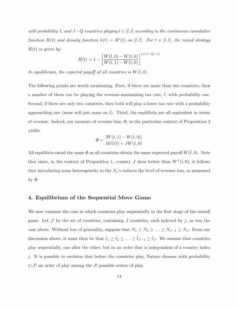
The following points are worth mentioning. First, if there are more than two countries, then
a number of them can be playing the revenue-maximizing tax rate, t, with probability one.
Second, if there are only two countries, then both will play a lower tax rate with a probability
approaching one (none will put mass on t). Third, the equilibria are all equivalent in terms
of revenue. Indeed, our measure of revenue loss, Φ, in the particular context of Proposition 2
yields:
Φ =[W (t, 1) − W (t, 0)]MtI(t) + JW (t, 0)
All equilibria entail the same Φ as all countries obtain the same expected payoff W (t, 0). Note
that since, in the context of Proposition 1, country J does better than W J(t, 0), it follows
that introducing some heterogeneity in the Nj ’s reduces the level of revenue loss, as measured
by Φ.
4. Equilibrium of the Sequential Move Game
We now examine the case in which countries play sequentially in the first stage of the overall
game. Let J be the set of countries, containing J countries, each indexed by j, as was the
case above. Without loss of generality, suppose that N1 ≥ N2 ≥ . . . ≥ NJ−1 ≥ NJ . From our
discussion above, it must then be that t1 ≥ t2 ≥ . . . ≥ tJ−1 ≥ tJ . We assume that countries
play sequentially, one after the other, but in an order that is independent of a country index
j. It is possible to envision that before the countries play, Nature chooses with probability
1/J ! an order of play among the J ! possible orders of play.
14

Before going further, it is useful to re-formulate our tie breaking rule for the case in which S
countries have chosen the same lowest tax rate. Our assumption is that in such a case, all
mobile capital M locates in the country with the largest index j. For example, if countries
2, 3, and 7 have set the lowest tax rate, then M locates in country 7. Such an assumption
reflects the fact that because tj is lower (not larger) for a higher index j (because it has a
smaller Nj), the country with the highest index is that which could ultimately undercut every
other countries.
In this sequential game, Lemmas 1 and 2 still hold, so for each country, equilibrium strategies
must belong to the real line [tj , t]. Let aj , j = 1, ..., J − 1, be an indicator function which
takes a value of 1 if country j chooses its tax rate after country J , and a value of 0 if it
chooses it before. We denote by A ⊂ J the set of countries who choose their tax rate after
J : A = {j ∈ J |aj = 1}. The following can be obtained.
Proposition 3: If tJ = min{tj , j ∈ J }, then the subgame perfect equilibrium of the tax
competition game is a strategy profile (t?1, . . . , t?J) in which all countries play the revenue-
maximizing tax rate (t?j = t, ∀ j 6= J), except for country J , which plays t?J = min{tk|k ∈ A}.
Thus, in all equilibria, mobile capital locates in country J , the one which can undercut every
other country. The presence of smallest country J disciplines all the larger countries, making
it useless for them to enter into tax competition and inducing them to maximize the revenue
yield of the immobile base. But the tax rates the smallest country must play to attract mobile
capital depends on the order of moves. The worse case scenario occurs when country J − 1
plays after country J (J − 1 ∈ A). In this case, of course, t?J = tJ−1, and so t?J may be
significantly smaller than t. The revenue loss stemming from the under-taxation of capital
may therefore be quite large. On the other hand, the best-case scenario occurs when country
J plays last (A = ∅). In such a case, t?J = t, so global tax revenue is maximized.
Clearly, the nature of the revenue loss in the sequential game is the same as that in the
15

simultaneous game. Our results can therefore be viewed as being robust to changes in the
timing of the game. However, there is only one country taxing capital below t in the sequen-
tial game, and two in the simultaneous game. Also note that in the sequential game, the
equilibrium outcome is uncertain ex ante because of the uncertainty regarding the order of
play, not because the countries play mixed strategies.
It turns out that calculating the appropriate measure of revenue loss in the sequential game
in the most general case of J countries is fairly involved. However, we know that in this
sequential game, all countries obtain W j(t, 0) for all order of moves, except for J which,
in the worse case scenario, when country J − 1 plays after country J , obtains a payoff of
W J(tJ−1, 1), and which does better for any other scenario in which country J −1 plays before
country J . Using our loss measure, Φ, we can immediately recognize two points: (a) The
level of loss in the worse case scenario of the sequential game is equal to that in the overall
simultaneous game; (b) This level of loss is less than that of the overall simultaneous game
in any other scenario of the sequential game. Since the worse case scenario occurs with a
probability less than one in the sequential game, it follows from this that there is less revenue
loss in the sequential game than in the simultaneous game, a result which is intuitive.
5. Discussion
5.1 Varying Productivities
As an extension to our analysis, we now want to examine the case in which the productivity
of investment varies across countries. Thus, suppose that the technology in each country is
given by Fj(K) = γjK, with γj > 0 being possibly different across countries. Recall from
above that the countries have been indexed by j so that N1 ≥ N2 ≥ ... ≥ NJ . Suppose that
the ordering of the γj is independent of the index j. Of particular interest to us is the country
with the largest γj . Let country g be this country: max{γi}Ji=1 = γg.
16

In this context, full efficiency requires that all countries tax at rate tj (which now differs for
different countries) and that mobile capital locates in the most productive country, i.e. in
country g.
Consider the case of a sequential move game. From what was shown in Section 4, it should
be clear that whatever the order of moves, mobile capital will locate in the country with the
largest per unit return γj − tj that a country can offer. It follows that capital will locate
inefficiently if maxj{γj − tj}Jj=1 6= g.
To see how this can happen, let ∆gj = γg−γj ≥ 0 be the difference in productivity between the
most productive country g and any other country j. Note that countries never set a negative
tax rate (tj ≥ 0) otherwise their payoff would be negative. It follows that if a country is so
unproductive that ∆gj > tg, then this country will never be able to attract mobile capital at
positive tax rate tj. This is reminiscent of the analysis of Cai and Treisman (2005) in which
countries of too low productivity are simply unable to compete for mobile capital. Thus, we
focus on countries that are sufficiently productive and for which ∆gj ≤ tg. Let J ′ ⊆ J be the
set of such countries. Now recall that the smaller the Nj of a country, the lower the smallest
tax rate tj it can offer. It should therefore be clear that some countries belonging to J ′,
despite being less productive than country g, may be small enough to attract mobile capital.
Indeed, let Ngj , j ∈ J ′, j 6= g, be the solution to the following implicit equation:
tgNg
Ng + M
I(γg − tg)I(γg − tg)
− tjNgj
Ngj + M
I(γj − tj)I(γj − tj)
− ∆gj = 0
It can then be shown that if ∃j ∈ J ′, j 6= g|Nj < Ngj , then there is a country that is small
enough to attract mobile capital despite being less productive than country g. In such a case,
all countries tax choose their revenue-maximizing tax rate, tj (including country g), except
the country in which mobile capital ends up locating. Thus, there is now not only the revenue
loss from taxing mobile capital at too low a rate, but also the potential inefficiency from
17

capital possibly ending up locating in a country where it is not the most productive.
To summarize, the presence of small and less productive countries generates two effects. On
the one hand, small and less productive countries discipline productive and large countries
and induce them to maximize the revenue yield of their immobile tax bases. On the other
hand, these small and less productive countries, by taxing capital at lower tax rates, may end
up with a disproportionately large share (all of it in our analysis) of mobile capital because
they are the ones who have less to lose from low taxes.
5.2 Preferential versus Non-Preferential Regimes
We now turn to a comparison of bilateral preferential regimes – i.e. regimes in which com-
peting countries can set different tax rates on bases of differing mobility – with bilateral
non-preferential regimes – i.e. regimes in which tax rates are constrained to be the same on
all bases. The main advantage of a preferential regime resides in the fact that governments
can avoid losing tax revenue on immobile tax bases by setting an appropriately high tax rate
on them, while competing more aggressively on the more mobile ones. On the other hand,
a non-preferential regime has the advantage of reducing competition on the mobile tax bases
by tying them to the more immobile ones. In other words, a non–preferential regime makes it
more costly for governments to lower their tax rates and so reduces harmful tax competition.
Depending on the environment, one or the other regime may be desirable. Janeba and Pe-
ters (1999), in an environment entailing one perfectly mobile base and one perfectly immobile
base, show that a non-preferential regime dominates a preferential regime. On the other hand,
Keen (2001) obtains the opposite result when two bases are at least partially mobile. Wilson
(2005) generalizes and attempts to reconcile these results within a unified framework.
It turns out that the framework developed in this paper can be used to contribute to this
literature. We focus on the simple case in which one tax base is perfectly mobile and the other
18

one is perfectly immobile. Since the equilibrium properties depend on whether countries set
their tax rates simultaneously or sequentially, we have to study each case in turn.
In the case of a simultaneous game, the non–preferential regime equilibrium tax rates are
the outcome of a mixed strategy Nash equilibrium in which countries choose their tax rates
in the manner stated in Proposition 1. In equilibrium, the expected tax revenue of each
country is given by W j(t, 0) (the same amount they would obtain by maximizing tax revenue
from their immobile base only) except for smallest country J which does better, obtaining
W J(tJ−1, 1) > W J(t, 0). In the case of a preferential regime, the characterization of the
equilibrium is a lot simpler. Since tax rates on mobile and immobile capital are disconnected,
our framework can be viewed as a simple first-price auction18. Thus, each country sets the
revenue maximizing tax rate t on its immobile base, and competition drives the tax rate on the
mobile base to zero. Tax revenue in that case is given by W j(t, 0) for all countries. It follows
that in the case of a simultaneous game, a non-preferential regime dominates a preferential
one since at least one country (country J) does better in the non-preferential one.
For the case of a sequential game, Proposition 3 establishes that in a non-preferential regime,
all countries obtain W j(t, 0) except for country J which obtains at least W J(tJ−1) ≥ W J(t, 0)
(with a strict inequality if NJ > NJ−1) and even better in a potentially large number of order
of moves. The analysis of the preferential regime in the sequential game is identical to that in
the simultaneous case. All countries set a tax rate t on immobile capital, but for the mobile
base, intense competition implies that the only subgame perfect equilibrium is for all countries
to set their tax rate at zero. The expected payoff for all countries is therefore W j(t, 0). Thus,
because at least one country (country J) does better in the non-preferential regime, we again
conclude that a non-preferential regime dominates a preferential one.
18 Recall that in the case of a non-preferential regime, in which tax rates are tied, our frameworkcan be interpreted as an all-pay auction.
19

But there are also, within our framework, arguments in favour of preferential regimes. Clearly,
since tax rates on mobile capital are driven down to zero in a preferential regime, the location
decision of mobile capital owners is unaffected by tax considerations and it must then be
that mobile capital will locate in the most productive country. Recall from the previous Sub-
section that mobile capital could locate inefficiently in a non-preferential regime. It follows
from this that non-preferential regimes are better at reducing the under-taxation of capital,
but that preferential regimes are better at eliminating the inefficiency associated with the
wrong location of mobile capital.
6. Conclusion
The current analysis could be extended in a few directions. First, we could assume that gov-
ernments care about new investment not only because of the resulting rise in tax revenue, but
also because of various external benefits such as employment gains in desirable occupations.
Keen (2001) discusses such an extension in his analysis of preferential and non-preferential
regimes, showing that his analysis can be generalized to encompass these additional benefits.
Similarly, we may amend the objective function to read
W j(t, 1) = (t + b)[Nj + M ]I(t)
W j(t, 0) = (t + b)NjI(t),
where b represents the external benefit per unit of investment. This extension reduces the tax
rate that is optimal for a country in the absence of mobile capital: countries no longer wish
to maximize revenue, because the investment loss resulting from a marginal increase in the
tax rate now not only lowers the tax base, but also reduces the external benefits associated
with investment. But the previous analysis goes through with t now redefined in this manner.
In particular, countries other than the two smallest decide not to compete for capital and
instead set their tax rates equal to this t (Proposition 1), and the other results are similarly
extended.
20
Alternatively, the objective function may be specified as a weighted sum of tax revenue and the
producers’ surplus received by the suppliers of capital to a region. This extension recognizes
that higher tax rates harm capital owners by reducing their income from capital. Once again,
the analysis goes through with t reduced below its revenue-maximizing level to reflect this
harm. Presumably, the weight given to producers’ surplus would reflect the political influence
of capital owners, perhaps through lobbying activities. A more complex extension would
be to allow the benefits of additional capital to differ between mobile and immobile capital.
This asymmetry complicates the calculation of mixed strategies and is therefore left to future
research.
Two other extensions appear to us as likely to generate interesting results. The first one
would be to introduce labour and political economy considerations in the analysis. Suppose
that workers in each country benefit from the presence of productive capital because of the
associated larger output and wages, but also because capital is taxed to finance the provision
of a public good. Then, if capital is highly mobile and unevenly owned by the workers of
various countries, then the choice of tax rates on capital in a given country will be driven by
strategic international considerations — as in the current paper, but also by the distribution
of capital ownership within the country.
A second extension of the current analysis would be to use the framework of Section 4 as
the within-period game of a multi-period dynamic game. To simplify, assume that both
investors and governments are myopic. Also assume that the countries have the same pro-
ductivity, but that they differ in terms of their number of local capital owners. Further,
suppose that Mt new mobile investors are born each period and that the location decision
they make at that time is irreversible – in effect, mobile investors locate and transform them-
selves into local capital investors. Hence, suppose that at time t, the countries have local
capital (N1,t, . . . , N`,t, . . . , NJ,t). Then, from our previous analysis, and whatever the order of
moves within period t, if country ` is that with the smallest amount of local capital investors,
21
capital investors Mt then end up locating in country ` at time t. Assuming investors are
infinitely-lived, it follows that at time t + 1, the countries will have local capital investors
(N1,t+1 = N1,t, . . . , N`,t+1 = N`,t + Mt, . . . , NJ,t+1 = NJ,t). Of course, it will again be the
country with the smallest number of local capital investors that will attract mobile capital
investors Mt+1. If this process continues, the smaller countries will become larger – while the
large ones will stagnate – and all countries will evolve to be approximately of the same size.19
Thus, the environment considered in this paper can generate convergence in the amount of
capital located in all countries. However, such a convergence does not seem to be happening
in the real world – e.g. see Table 1. We speculate that if investors and/or governments were
forward-looking – instead of being myopic – then convergence would not necessarily obtain.
These extensions of the current paper will be examined in future work.
19 The difference between the size of the largest country and that of the smallest of course dependson the size of the elements of the sequence {Mt,Mt+1, . . .}.
22

7. Appendix: Proofs
Proof of Lemma 1: For any t′i > t, there exists a t′′i < t such that W i(t′′i ,m) = W i(t′i,m),
for m ∈ {0, 1}. Of course, since under t′′i , the country is more likely to attract the mobile
capital, it will always prefer to play t′′i . QED.
Proof of Lemma 2: If a country plays ti < ti and all the mobile capital locates on its
territory, it will get a payoff which is less that it gets when it taxes at rate t and no mobile
capital locates on its territory: W i(ti < ti, 1) < W i(t, 0). QED.
Proof of Lemma 3: (A) We first study the case of two identical countries. For Ni = Nj ,
we first show that there is no symmetric (ti = tj) pure strategy Nash equilibrium and then
show that there is no asymmetric (ti > tj) pure strategy Nash equilibrium.
(i) There is no symmetric (ti = tj) pure strategy Nash equilibrium.
Consider a strategy profile (t, t), with t ∈ [t, t] (from Lemma 1 and Lemma 2).
If t > t, then the payoff of each country is W 1 = W 2 = 12W (t, 1) + 1
2W (t, 0). Clearly, this
cannot be an equilibrium as any country, say 1, has an incentive to deviate to t′1 = t− ε ≥ t,
causing all the capital to locate in 1, and ensuring itself a payoff W 1′= W (t − ε, 1) > W 1.
If t = t, then the payoff of each country is W 1 = W 2 = 12W (t, 1) + 1
2W (t, 0). Clearly, this
cannot be an equilibrium as any country, say 1, has an incentive to deviate to t′1 = t, ensuring
itself a payoff W 1′= W (t, 0) > W 1.
(ii) There is no asymmetric (ti > tj) pure strategy Nash equilibrium.
Consider any strategy profile (t1, t2), with t ≥ t1 > t2 ≥ t.
If t ≥ t1 > t2 > t, then W 1 = W (t1, 0) and 1 has an incentive to deviate to t′1 = t2 − ε > t to
23

obtain W 1′= W (t2 − ε, 1) > W 1.
If t > t1 > t2 = t, then W 1 = W (t1, 0) and 1 has an incentive to deviate to t′1 = t to obtain
W 1′= W (t, 0) > W 1.
If t = t1 > t2 = t, then W 2 = W (t, 1) and 2 has an incentive to deviate to t′2 = t − ε > t to
obtain W 2′= W (t − ε, 1) > W 2.
This completes part (A) of the proof.
(B) We now turn to the case in which there are two countries with Ni > Nj .
From above, we know that ti > tj . As Lemma 1 and Lemma 2 apply when Ni > Nj , it
follows that the strategies of the countries must belong to the following intervals: ti ∈ [ti, t]
and tj ∈ [tj, t].
We first show that there is no symmetric (ti = tj) pure strategy Nash equilibrium and then
show that there is no asymmetric (ti 6= tj) pure strategy Nash equilibrium.
(i) There is no symmetric (ti = tj) pure strategy Nash equilibrium.
Since tj < ti < t, a symmetric equilibrium is a pair (t, t) such that t ∈ [ti, t]. Consider such a
strategy profile (t, t).
If t > ti, then the payoff of country i is W i = 12W i(t, 1) + 1
2W i(t, 0) and that of j is W j =
12W j(t, 1) + 1
2W j(t, 0). Clearly, this cannot be an equilibrium as any country, say i, has an
incentive to deviate to t′i = t− ε ≥ ti, causing all the capital to locate in i, and ensuring itself
a payoff W i′ = W i(t − ε, 1) > W i.
If t = ti, then the payoff of country i is W i = 12W i(ti, 1) + 1
2W i(ti, 0) and that of j is
W j = 12W j(ti, 1) + 1
2W j(ti, 0). Clearly, this cannot be an equilibrium as i has an incentive
to deviate to t′i = t ensuring itself a payoff W i′ = W i(t, 0) > W i.
24

(ii) There is no asymmetric (ti 6= tj) pure strategy Nash equilibrium.
Without loss of generality, assume that N1 > N2 so that t2 < t1 < t.
Consider a strategy profile (t1, t2) with t1 ≤ t1 < t2 ≤ t. Given those strategies, W 1 =
W 1(t1, 1) and W 2 = W 2(t2, 0). Then, 2 has an incentive to deviate to t′2 = t1 − ε to obtain
W 2′= W 2(t1 − ε, 1) > W 2.
Consider a strategy profile (t1, t2) with t2 < t1 < t2 < t1 ≤ t. Given those strategies,
W 1 = W 1(t1, 0) and W 2 = W 2(t2, 1). Then, 1 has an incentive to deviate to t′1 = t2 − ε to
obtain W 1′= W 1(t2 − ε, 1) > W 1.
Consider a strategy profile (t1, t2) with t2 ≤ t2 ≤ t1 < t1 < t. Given those strategies,
W 1 = W 1(t1, 0) and 1 has an incentive to deviate to t′1 = t to obtain W 1′= W 1(t, 0) > W 1.
Consider a strategy profile (t1, t2) with t2 ≤ t2 < t1 ≤ t1 < t. Given those strategies,
W 1 = W 1(t1, 0) and 1 has an incentive to deviate to t′1 = t to obtain W 1′= W 1(t, 0) > W 1.
Consider a strategy profile (t1, t2) with t2 ≤ t2 ≤ t1 < t1 = t. Given those strategies, W 2 =
W 2(t2, 1) and 2 has an incentive to deviate to t′2 = t− ε to obtain W 2′= W 2(t − ε, 1) > W 2
for ε small.
This completes part (B) of the proof.
(C) The generalization of (A) and (B) to the case of J countries with N1 ≥ N2 ≥ ... ≥ NJ is
tedious but straightforward.
This completes the proof. QED.
Proof of Proposition 1: Because N1 > N2 > ... > NJ−1 > NJ , we have 0 < tJ < tJ−1 <
... < t2 < t1 < t. The equilibrium strategies are as follows.
25

� Countries j = 1, ..., J − 2: Play t with probability qj = 1.
� Country J − 1: With positive probability qJ−1 ∈ ]0, 1[ , plays t; with positive probability
(1− qJ−1), plays the interval [tJ−1, t[ with continuous probability distribution HJ−1(t), with:
qJ−1 = 1 −[W J(t, 1) − W J(tJ−1, 1)
W J (t, 1) − W J(t, 0)
]
HJ−1(t) =[W J(t, 1) − W J(tJ−1, 1)] [W J(t, 1) − W J(t, 0)][W J(t, 1) − W J(t, 0)] [W J(t, 1) − W J(tJ−1, 1)]
� Country J : Plays the interval [tJ−1, t[ with continuous probability distribution HJ(t), with:
HJ(t) =W J−1(t, 1) − W J−1(t, 0)W J−1(t, 1) − W J−1(t, 0)
Thus, all countries except the two smallest ones (J − 1 and J) put themselves out of the race
to attract mobile capital by taxing at rate t with probability one. Mobile capital locates in
country J − 1 or J .
In equilibrium, the expected payoff of all countries (except J) is equal to that they obtain
when unable to attract mobile capital and taxing immobile capital at the revenue-maximizing
tax rate, t, i.e. the expected payoff for j = 1, ..., J − 1 is W j(tj, 1) = W j(t, 0). The sole
country which does better is country J , the smallest one. It obtains and expected payoff of
W J(tJ−1, 1) > W J(tJ , 1) = W J (t, 0).
The proof that these strategies constitute an equilibrium is simply that given the other coun-
tries’ strategy, Country j has no desire to deviate.
To determine qJ−1, HJ−1(t), and HJ(t), the procedure is as follows.
(A) Consider first the payoffs for country J for some of its pure strategies, given the strategy
of country J − 1. Note that since the other countries always play t, they have no impact on
the payoff of country J .
26

A.1 When country J plays tJ−1, it obtains W J(tJ−1, 1):
qJ−1WJ(tJ−1, 1) + (1 − qJ−1)[HJ−1(tJ−1)W J (tJ−1, 0) + (1 − HJ−1(tJ−1))W J (tJ−1, 1)]
= W J(tJ−1, 1)
A.2 For any t ∈]tJ−1, t[ , country J obtains:
qJ−1WJ(t, 1) + (1 − qJ−1)[HJ−1(t)W J (t, 0) + (1 − HJ−1(t))W J (t, 1)]
Imposing that this last expression equals W J(tJ−1, 1) to ensure that all pure strategies yield
the same payoff, we can solve for HJ−1(t):
HJ−1(t) =W J (t, 1) − W J(tJ−1, 1)
(1 − qJ−1)[W J(t, 1) − W J(t, 0)]
It is easily checked that HJ−1(tJ−1) = 0. Using the fact that lim t→t HJ−1(t) = 1, we can
solve for qJ−1 and obtain:
qJ−1 = 1 −[W J(t, 1) − W J (tJ−1, 1)
W J(t, 1) − W J(t, 0)
]
Substituting this value of qJ−1 in HJ−1(t) above we get the following:
HJ−1(t) =[W J(t, 1) − W J(tJ−1, 1)] [W J(t, 1) − W J(t, 0)][W J(t, 1) − W J(t, 0)] [W J(t, 1) − W J(tJ−1, 1)]
And it is easily checked that HJ−1(tJ−1) = 0 and lim t→t HJ−1(t) = 1.
(B) Consider now the payoffs for country J−1 for any of its pure strategies given the strategy
of country J and that of the other countries.
For any t ∈ [tJ−1, t[ , country J − 1 obtains:
HJ(t)W J−1(t, 0) + (1 − HJ(t))W J−1(t, 1)
27
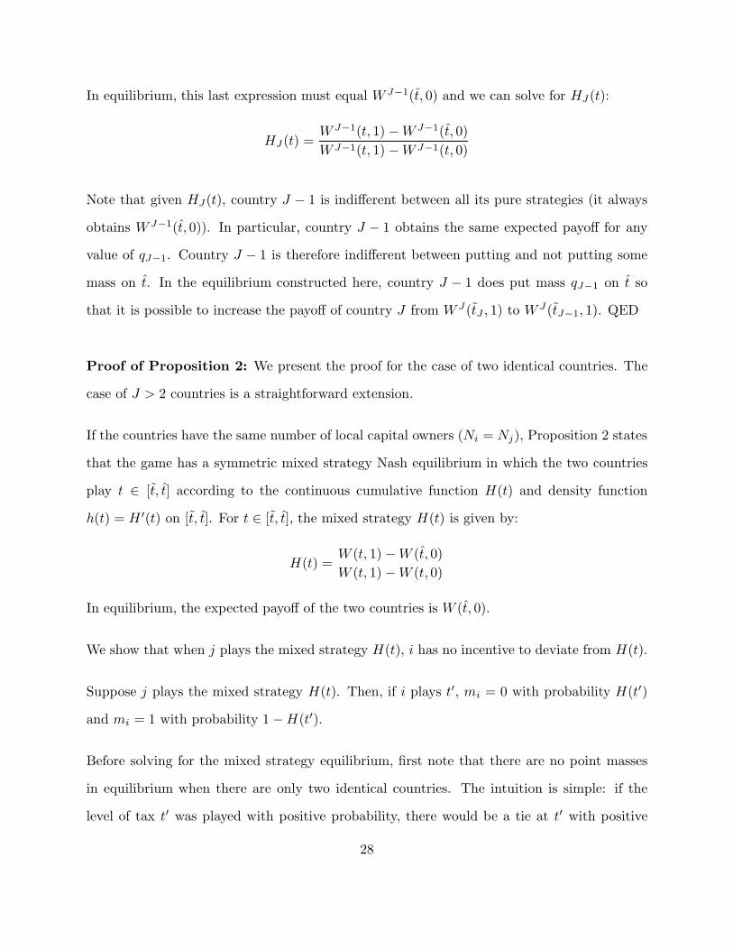
In equilibrium, this last expression must equal W J−1(t, 0) and we can solve for HJ(t):
HJ(t) =W J−1(t, 1) − W J−1(t, 0)W J−1(t, 1) − W J−1(t, 0)
Note that given HJ(t), country J − 1 is indifferent between all its pure strategies (it always
obtains W J−1(t, 0)). In particular, country J − 1 obtains the same expected payoff for any
value of qJ−1. Country J − 1 is therefore indifferent between putting and not putting some
mass on t. In the equilibrium constructed here, country J − 1 does put mass qJ−1 on t so
that it is possible to increase the payoff of country J from W J(tJ , 1) to W J(tJ−1, 1). QED
Proof of Proposition 2: We present the proof for the case of two identical countries. The
case of J > 2 countries is a straightforward extension.
If the countries have the same number of local capital owners (Ni = Nj), Proposition 2 states
that the game has a symmetric mixed strategy Nash equilibrium in which the two countries
play t ∈ [t, t] according to the continuous cumulative function H(t) and density function
h(t) = H ′(t) on [t, t]. For t ∈ [t, t], the mixed strategy H(t) is given by:
H(t) =W (t, 1) − W (t, 0)W (t, 1) − W (t, 0)
In equilibrium, the expected payoff of the two countries is W (t, 0).
We show that when j plays the mixed strategy H(t), i has no incentive to deviate from H(t).
Suppose j plays the mixed strategy H(t). Then, if i plays t′, mi = 0 with probability H(t′)
and mi = 1 with probability 1 − H(t′).
Before solving for the mixed strategy equilibrium, first note that there are no point masses
in equilibrium when there are only two identical countries. The intuition is simple: if the
level of tax t′ was played with positive probability, there would be a tie at t′ with positive
28
probability. Imagine then that country j decides to play t′ − ε (instead of t′) with the same
probability. The cost of such a deviation would be of the order of ε, but if the two countries
were to tie, then country j would gain a fixed positive amount. The formal proof of this is as
follows. Imagine that country i plays t′ with positive probability ω, and country j deviates
from t′ to t′ − ε with the same positive probability. The payoff for country j will change by
a factor of:
{Pr(ti < t′ − ε)W (t′ − ε, 0) − Pr(ti < t′)W (t′, 0)
}
+{
Pr(ti > t′ − ε)W (t′ − ε, 1) − Pr(ti > t′)W (t′, 1)}
+{
ωW (t′ − ε, 1) − ω
2[W (t′, 1) + W (t′, 0)]
}
The first terms in curly brackets represent the difference between losing with a tax level t′−ε,
and losing with a tax level t′. As for the second terms in curly brackets, they represent the
difference between winning with a tax level t′ − ε, and winning with a tax level t′. It is easy
to see that the sum of those terms goes to zero when ε goes to zero. Now, the last terms
in curly brackets represent the difference between winning alone with t′ − ε, and sharing the
win with t′. Since the sum of these terms is strictly positive when ε goes to zero, it pays to
deviate to t′ − ε when there is a probability mass at t′. This implies that H(t) cannot have
a probability mass.20 And because the cumulative function is continuous, cases in which the
countries play ti = tj (a tie) occur with probability 0.
We now solve for H(t) knowing that it must be continuous on [t, t]. Thus, given j plays H(t),
when i plays the mixed strategy H(t), its expected payoff is:∫ t
t
[H(z)W (z, 0) + (1 − H(z))W (z, 1)] dH(z)
20 Note that a different argument is required to show that there cannot be a probability mass at t.The argument goes as follows. Suppose that each country plays t with probability ω. There isthen a positive probability that the countries will tie at t and earn a strictly dominated payoff:1/2[W (t, 1) + W (t, 0)] < W (t, 0). Thus, H(t) cannot have a mass at t.
29

For (H(t),H(t)) to be a mixed strategy Nash equilibrium, it has to be that all pure strategies
played with positive probability yield the same payoff. We construct the equilibrium so that
the expected payoff of the two countries is W (t, 0). Thus, it has to be that:
H(t)W (t, 0) + (1 − H(t))W (t, 1) = W (t, 0) ∀ t ∈ [t, t]
It follows that for t ∈ [t, t], H(t) is given by:
H(t) =W (t, 1) − W (t, 0)W (t, 1) − W (t, 0)
When j plays the mixed strategy H(t), i has no incentive to deviate from H(t) because:
- Changing the probability of playing any t ∈ [t, t] would not affect its payoff as all pure
strategies are equivalent by construction.
- Playing t ∈ [0, t[ or t ∈]t,∞] with positive probability would decrease i’s expected payoff
as these strategies are all dominated (Lemma 1 and Lemma 2).
This completes the proof for the case of two identical countries. It is easily shown that for
the case of J > 2 countries, either all countries play a modified H(t) given by
H(t) = 1 −[W (t, 0) − W (t, 0)W (t, 1) − W (t, 0)
]1/(J−Q−1)
or some of them (Q ≤ J − 2) put a unit mass on t. QED.
Proof of Proposition 3: (A) We first study the case of two countries, 1 and 2, with N1 ≥ N2.
We start by examining the case in which country 2 plays first. In that case, the game has a
pure perfect Nash equilibrium in which country 2 sets t2 = t1 and country 1 sets t1 = t. In
equilibrium, mobile capital locates in 2 and the payoff of country 1 is W 1(t, 0) while that of
country 2 is W 2(t1, 1) > W2(t, 0).
30

To see that this must be true, note that because country 2 has a lower N2, it has a lower t:
t2 ≤ t1. Consequently, country 2 can always and does undercut country 1 by setting t2 = t1
(recall our breaking rule). Country 1 then chooses the best tax rate available given it is unable
to compete, i.e the tax rate it chooses when isolated: t.
Consider now the case in which country 1 plays first. In that case, the game has a pure perfect
Nash equilibrium in which both countries play t. In equilibrium, mobile capital locates in 2
and the payoff of countries 1 is W 1(t, 0) while that of country 2 is W 2(t, 1). To see that this
must be true, recall that country 1 can always be undercut by country 2. Country 1 thus sets
t1 = t and country 2, benefiting from the breaking rule, plays t2 = t.
This completes part (A) of the proof.
(B) The generalization of (A) to the case of J countries with N1 ≥ N2 ≥ ... ≥ NJ is
straightforward. QED.
31

8. References
Aiyar S., and C.J. Dalgaard (2001), “Total Factor Productivity Revisited: A Dual Approach
to Levels-Accounting,” mimeo.
Auerbach, A.J. (2005), “Who bears the Corporate Tax? A Review of What We Know”,
Working Paper 11686, NBER.
Baldwin, R.E., and P. Krugman (2004), “Agglomeration, Integration and Tax Harmonisa-
tion,” European Economic Review 48, 1–23.
Baye, M.R., D. Kovenock, and C.G. de Vries (1996), “The All-Pay Auction With Complete
Information”, Economic Theory 8, 291–305.
Boadway, R., K. Cuff, and N. Marceau (2004), “Agglomeration Effects and the Competition
for Firms,” International Tax and Public Finance 11, 623–645.
Bucovetsky, S. (1991), “Asymmetric Tax Competition,” Journal of Urban Economics 30,
167–181.
Cai, H., and D. Treisman (2005), “Does Competition for Capital Discipline Governments?
Decentralization, Globalization, and Public Policy”, American Economic Review 95, 817–
830.
Dasgupta, P., and E. Maskin (1986), “The Existence of Equilibrium in Discontinuous Eco-
nomic Games II: Applications”, Review of Economic Studies 53, 27–41.
Edwards, J., and M. Keen (1996), “Tax Competition and Leviathan,” European Economic
Review 40, 113–134.
Haufler, A. (2001), Taxation in a Global Economy, Cambridge: Cambridge University Press.
Hines, J.A. (2005), “Corporate Taxation and International Competition,” mimeo, University
of Michigan.
Janeba, E., and W. Peters (1999), “Tax Evasion, Tax Competition and the Gains from Nondis-
crimination: The Case of Interest Taxation in Europe”, Economic Journal 109, 93–101.
Janeba, E., and M. Smart (2003), “Is Targeted Tax Competition Less Harmful Than Its
32

Remedies,” International Tax and Public Finance 10, 259–280.
Kanbur, R., and M. Keen (1993), “Jeux sans frontieres: Tax Competition and Tax Coordi-
nation when Countries Differ in Size,” American Economic Review 83, 877–892.
Keen, M. (2001), “Preferential Regimes Can make Tax Competition Less Harmful”, National
Tax Journal 54, 757–762.
Kind, H.J., K.H.M. Knarvik, and G. Schjelderup (2000), “Competing for Capital in a ‘Lumpy’
World”, Journal of Public Economics 78, 253–274.
Kreps, D.M., and J.A. Scheinkman (1983), “Quantity Precommitment and Bertrand Compe-
tition Yield Cournot Outcomes”, Bell Journal of Economics 14, 326–227.
Levitan, R., and M. Shubik (1972), “Price Duopoly and Capacity Constraints”, International
Economic Review 13, 111–122.
OECD (1998), Harmful Tax Competition: An Emerging Global Issues, Paris: OECD.
Slemrod, J., and J.D. Wilson (2006), “Tax Competition with Parasitic Tax Havens,” mimeo,
Michigan State University.
Sørensen, P.B. (2000), “The Case for International Tax Co-Ordination Reconsidered”, Eco-
nomic Policy 31, 429–272.
Summers, R., and A. Heston (1991), “The Penn World Table (Mark 5): An Expanded Set of
International Comparisons, 1950-1988”, Quarterly Journal of Economics 106, 327–368.
Trefler, D. (1993), “International Factor Price Differences: Leontief Was Right!”, Journal of
Political Economy 101, 961–987.
Varian, H.R. (1980), “A Model of Sales”, American Economic Review 70, 651–659.
Wilson, J.D. (1986), “A Theory of Interregional Tax Competition,” Journal of Urban Eco-
nomics 19, 296–315.
Wilson, J.D. (1991), “Tax Competition with Interregional Differences in Factor Endowments,”
Regional Science and Urban Economics 21, 423–451.
Wilson, J.D. (1999), ”Theories of Tax Competition,” National Tax Journal 52, 269–304.
Wilson, J.D. (2005), “Tax Competition with and without Preferential Treatment of a Highly-
33

Mobile Tax Base,” In J. Alm, J. Martinez-Vasquez, and M. Rider, Editors, The Challenge
of Tax Reform in a Global Economy, Springer.
Zodrow, G.R. and P. Mieszkowski (1986), “Pigou, Tiebout, Property Taxation, and the Un-
derprovision of Local Public Goods,” Journal of Urban Economics 19, 356–370.
34
9. Table and Figure
Table 1Effective average tax rate on capital, Productivity of capital,Capital stock per worker, and Population, for the EU and US
Effective average tax Productivity of capital Capital stock per Populationrate on capital (%) (as % of that in US) worker (US dollars) (millions)
1981 1991 1983 1985 1990
Austria 21.5 22.7 0.56 28245 7.7Belgium 39.5 36.0 0.66 42670 9.9Denmark 47.8 40.0 0.72 30878 5.1Finland 35.2 45.2 0.66 46451 4.9France 28.4 24.8 0.63 38093 56.7West Germany 31.0 26.5 0.68 38261 63.2Ireland 11.4 11.1 0.49 22741 3.5Italy 25.3 34.5 0.53 32968 56.7Netherlands 29.7 31.9 0.77 N/A 14.9Spain 13.9 20.3 0.53 26221 39.3Sweden 47.4 53.1 0.97 25256 8.5United Kingdom 66.5 45.3 0.84 22600 56.7
EU average 33.1 32.6 0.67 32217 27.2
United States 40.9 41.1 1.00 32046 285.1
Notes: Except for the effective tax rate on capital income, EU average is that of the countries listed in this
table.
Sources: Effective tax rate on capital income: Sørensen (2000, Table 2) or Haufler (2001, Table 4.1). Produc-
tivity of Capital: Trefler (1993, Table 1). Capital stock per worker: Summers and Heston (1991, Table II).
Population: United Nations Population Division website (http://esa.un.org/unpp/).
35

t
W
0
W j(t, 1)
W j(t, 0)
•
••
•
W j(t, 1)
W j(t, 0) = W j(tj , 1)
W j(tj , 0)
t ttj
........................................................................................................................................................................................................................................................................................................................................................................................................................................................................................................................................................................................................................................................................................................................................................................................................................................................................................................................................................................................................................................................................................................................................................
................................................................................................................................................................................................................................................................................................................................................................................................................................................................................................................................................................................................................................................................................................................................................................................................................................................................................................................................................................................................................................................................................................................................................................................................................................................................................................................................................................................................................................................................................................................................................................................................................................................................................................................................
........................................................................................................................................................................................................................................................................................................................................................................................................................................................................................................................................................
....................................................................................................................................................................
.....................................................................................................................................................................................................................................................................................................................................................................................................................................................................................................................................................................................................................................................................................................................................................................................................................................................................................................................................................................................................................................................................................................................
...............................................................................................................
.....................
.........................................................................................................
.....................
........
.....
........
.....
........
.....
........
.....
........
.....
........
.....
........
.....
........
.....
........
.....
........
.....
........
.....
........
.....
........
.....
........
.....
........
.....
........
.....
........
.....
........
.....
........
.....
........
.....
........
.....
........
.....
........
....
............................................................................................................................................................................
............................................................................................................................................................................
.............
.............
.............
.............
.............
.............
.............
.............
.............
.............
.............
......
....................................................
Figure 1: The Payoffs
36