Finance and Economics Discussion SeriesDivisions of Research & Statistics and Monetary Affairs

Federal Reserve Board, Washington, D.C.

Why Do Innovative Firms Hold So Much Cash? Evidence fromChanges in State R&D Tax Credits

Antonio Falato and Jae Sim

2014-72

NOTE: Staff working papers in the Finance and Economics Discussion Series (FEDS) are preliminarymaterials circulated to stimulate discussion and critical comment. The analysis and conclusions set forthare those of the authors and do not indicate concurrence by other members of the research staff or theBoard of Governors. References in publications to the Finance and Economics Discussion Series (other thanacknowledgement) should be cleared with the author(s) to protect the tentative character of these papers.

Why Do Innovative Firms Hold So Much Cash?Evidence from Changes in State R&D Tax Credits

Antonio FalatoFederal Reserve Board1

Jae W. SimFederal Reserve Board

This Draft: May 2014

1Corresponding author: Antonio Falato, Federal Reserve Board, 20th st & Constitution Av NW WashingtonDC 20511 Phone: (202) 452-2861. Email: antonio.falato@frb.gov. We thank Kai Li, Mitchell Petersen, GordonPhillips, David Scharfstein, and seminar participants at the Federal Reserve Board for helpful comments anddiscussions. Special thanks to Darrell Ashton for his help with parsing the SEC filings, to Tim Loughran andJay Ritter for making their sample of seasoned equity offerings available to us, and to Daniel Wilson and BobChirinko for kindly sharing their hand-collected data on state-level investment tax credits. Suzanne Changprovided excellent research assistance. All remaining errors are ours.

Abstract

This paper uses the staggered changes of R&D tax credits across U.S. states and over time as a quasi-

natural experiment to examine the impact of innovation on corporate liquidity. By generating plau-

sibly independent variation in firms’ incentive to invest in R&D, we are able to assess the empirical

importance of specific theories of the link between innovation and corporate liquidity. Firms increase

(decrease) their cash to asset ratios by about one and a half percentage point when their home state

increases (cuts) R&D tax credits. These baseline difference-in-differences estimates hold up to a bat-

tery of validation, falsification, and robustness checks, which corroborate their internal and external

validity. The treatment effect of R&D tax credits increases monotonically with several specific prox-

ies for debt and equity financing frictions. Increases (cuts) in tax credits also lead to increases (de-

creases) in the ratios of cash to bank lines of credit and to book equity, and to decreases (increases) in

bank debt, secured debt, and overall net indebtness, supporting debt and equity financing channels

through which innovation impacts the demand for cash. We also find support for a product market

competition channel, and assess repatriation and agency explanations. Overall, our analysis offers

endogeneity-free evidence that innovation is a first-order driver of corporate liquidity management

decisions.

1 Introduction

That the top U.S. cash holders are innovative corporations which rely heavily on R&D investments

is well-known and to be expected based on first principles in corporate finance (for example, Aghion

and Tirole (1994), Hart and Moore (1994)). In fact, innovative corporations held, on average, as much

as a third of their assets in cash or near-cash instruments over the last decade, and the five largest

cash holders were Apple, Microsoft, Google, Cisco, and Pfizer, who held more than one quarter of the

total cash of the U.S. corporate sector. Especially since U.S. corporate cash holdings hit new record

highs after the financial crisis, the subject of cash holdings of innovative firms has made headlines

in the press and received attention by policy makers and institutional shareholder activists, with the

likes of Carl Ichan and David Einhorn pressuring innovative firms to disgorge their cash.1

However, what is relatively less well understood and remains actively debated is the question of

why innovative firms hold so much cash. Is it because innovation matters for cash, or is it because

innovative firms are just fundamentally different from the average U.S. corporation along observable

and unobservable dimensions that are hard to control for? In addition, if innovation matters, how

does it matter – i.e., through which channels does it impact cash? Despite the small yet growing

literature on the financial economics of innovation, which has been generally focused on external

rather than internal financing (Brown et al (2009; 2013), Chava et al (2013); Hall and Lerner (2010) is

a survey), and the vast literature on the determinants of cash, which, starting from Opler et al (1999),

has generally included R&D as a covariate for a large cross-section of firms, to date there has been no

attempt at empirically identifying the impact of innovation on cash and at systematically evaluating

the channels.

In order to fill the gap in the literature, we design a quasi-natural experimental setting that over-

comes the empirical identification challenge of finding plausibly exogenous sources of variation in

innovation by exploiting staggered changes in R&D tax credits across U.S. states and over time. One

of the challenges with cross-sectional estimates is that measures of innovation are also correlated with

proxies for why innovation matters, which complicates the examination of how innovation impacts

corporate liquidity. By generating variation in firms’ incentives to invest in R&D that is plausibly un-

related to firm-level characteristics, our quasi-experimental design also helps to overcome this issue.

In summary, we offer well-identified estimates of the impact of innovation on cash, direct evidence

that innovation is a first-order determinant of corporate liquidity, and a comprehensive assessment

1See, for example, "Too Much Cash Isn’t Good for Apple," BusinessWeek, February 26, 2013.

1

of the specific channels through which innovation impacts cash.

We start with presenting descriptive evidence that there is a positive cross-sectional relation be-

tween measures of firm innovation based on R&D expenditures and cash holdings relative to assets

as well as external liquidity (bank lines of credit) in a standard panel of U.S. firms between 1986

and 2011. This evidence, which replicates in our sample the findings of Opler et al (1999) and Bates,

Kahle, and Stulz (2009) for cash and Sufi (2009) for lines of credit, is important, but its interpretation

is limited by a variety of well-known endogeneity concerns. In particular, when measuring the ef-

fect of innovation using comparisons across firms, there will always be a suspicion that the controls

included in the analysis are not exhaustive. Such concerns are mitigated when the specification in-

cludes firm fixed effects. Nevertheless, if there are time-varying omitted firm characteristics, such

as future profit growth opportunities, that affect both the firm’s incentives to invest in R&D and its

cash holdings decisions, then the estimates would not have a causal interpretation. As such, the

cross-sectional evidence lays out the foundation for our effort to take a first step toward identifying

the causal link between R&D and cash, and assessing the empirical relevance of the theories that can

explain the link.

To achieve identification, we exploit plausibly exogenous time-series variation in firms’ incentives

to innovate that arises due to changes in state R&D tax credits.2 By way of validation, we show

that R&D expenses respond strongly to changes in state R&D tax credits, which is in line with the

existing evidence on the effectiveness of tax incentives for R&D (see Hall and Van Reenen (2000) for

a survey). In our baseline specification, we use a standard difference-in-difference (DID) approach

to derive estimates of the effect of changes in state R&D tax credits on cash holdings. To insure that

there are no systematic differences between treated and control firms that are relevant for their cash

holding decisions, which is our key identifying assumption, we include an extensive set of controls

for unobserved, time-invariant heterogeneity across firms; unobserved, time-varying heterogeneity

across industries ("industry shocks"); and firm level changes in other determinants of cash holdings.3

The inclusion of these controls insures that our estimates are identified by comparing the differential

(within-firm) response of cash holdings in the same industry-year for similar firms located in state-

years when there is a change in the R&D tax credit (the ’treatment group’) relative to those that are

2Over the last two decades, nearly every U.S. state has enacted some type of tax incentive for R&D andsubsequently repealed, reduced, or expanded.

3To minimize the risk of biases arising from the inclusion of potentially endogenous variables as per the"bad controls" problem discussed in Angrist and Pischke (2009), we include the pre-treatment (lagged) valuesof the firm-level variables.

2

not (the ’control group’).

Any residual identification concern about the internal validity of our baseline estimates can only

come from residual unobserved, time-varying heterogeneity across states that is not captured by the

industry-year effects, which may bias our estimates if it coincides with changes in state R&D tax

credits and is relevant for cash holding decisions.4 We take several steps to build confidence that our

estimates are well-identified. First, we implement validation tests of the main residual threat to our

identification by examining the determinants of states’ likelihood of changing their R&D tax credits,

which we allow to be a function of state-level variables that, on an a-priori basis, we expect may be

relevant for cash holding decisions, such as state business cycle and political conditions, labor market

forces, and other state taxes. The results of these validation tests indicate that the introduction of R&D

tax credits is the only type of change that is systematically related to state economic conditions and,

in general, to state-level variables, while increases or cuts of R&D tax credits subsequent to their

introduction appear generally unresponsive to state-level variables. Based on these results, we take

a conservative approach in our baseline analysis and only include in the treatment group changes

in state R&D tax credits subsequent to their introduction.5 Throughout the analysis, we take several

additional steps to address potential state-level confounds and bolster a causal interpretation of our

DID estimates, which include falsification and a battery of sensitivity tests.

Our baseline DID estimates indicate that there is an increase (decrease) in cash to book assets of

about 2 (1.7) percentage points after an increase (decrease) in R&D tax credits, a result which is robust

to using alternative definitions of cash ratios.6 To build confidence that these baseline estimates are

well-identified, we implement two batteries of falsification tests.7 First, we repeat our analysis for

two different sub-sample splits of the data based on proxies for the institutional design of the R&D

tax credits that should affect their effectiveness because of the way they affect the opportunity-cost

of R&D. The estimates indicate that there are strong and significant effects only for firms that are

4The reason why this issue is a potential challenge for our identification strategy is that it potentially threat-ens our key identifying assumption of "parallel trends" by which we are effectively assuming that absent achange in the state R&D tax credit, treated firms’ cash would have evolved in the same way as that of controlfirms. Thus, we need to address potential state level confounds that affect firms’ demand for cash irrespectiveof the R&D tax credits’ changes.

5Since we recognize that tax credit introductions, though less suitable for standard DID research design,are potentially interesting discrete events, we examine their impact in an extensive set of dedicated robustnesstests.

6There is no evidence of either firm anticipation or pre-event trends, while we also present evidence thatlarger tax credit changes trigger larger responses in cash.

7The specifications for both tests are all estimated in first differences to remove firm fixed effects in thelevels equations, and lagged changes in the firm-level controls of the baseline specification (1) as well as year-industry(48-FF) dummies are included.

3

subject to a stronger treatment. Second, we implement falsification tests that exploit changes in state

investment tax credits, which are state-level tax incentives programs otherwise analogous to the R&D

tax credits except for the fact that they give tax relief for capex – i.e., for investment in PPE, such as

plants, machinery, and buildings.8 The response of cash to changes in investment tax credits, though

somewhat weaker in magnitude, is qualitatively the exact opposite of the response to R&D credits,

with cash decreasing (increasing) in response to increases (cuts) in investment tax credits.

We implement an extensive set of sensitivity tests to further corroborate both the internal and ex-

ternal validity of our baseline estimates. First, we estimate versions of our baseline DID regressions

that use alternative standard errors9 and add more firm-, state-, and industry-level control variables,

such as state fixed effects to control for unobserved time-invariant differences among states. Sec-

ond, in an attempt to sharpen our identification, we refine the control group to include only firms in

neighboring counties across border (see Homes (1998) for a similar approach) for which we can ex-

ploit the natural geographic discontinuity of tax policy (i.e., the fact that it stops at the state’s border)

to difference out unobserved variation in local economic conditions.10 Third, we consider robustness

to alternative estimators and asses the external validity of our baseline estimates. One of the alter-

native estimators we consider is a matched-sample DID estimator (Heckman, Ichimura, and Todd

(1997)) that replicates the DID tests after matching treated and control firms based on pre-treatment

characteristics that include state business cycle conditions, which further addresses the concern that

differences between treated and control firms may invalidate our parallel-trend assumption.11 To ex-

amine external validity, we include R&D tax credit introduction events in the treatment group. Our

estimates remain stable across different specifications, estimators, and types of treatments. Overall,

the results of our falsification, sensitivity, and external validity tests support a causal interpretation

of the observed response of cash.

In the second part of our analysis, we investigate the drivers of the treatment effect by examining

8Chirinko and Wilson (2008) hand-collected state-level data on these programs and show evidence of theireffectiveness at stimulating physical capital expenditures. We use their data to construct indicator variablesfor changes in state investment tax credits, which consist of 18 introduction events, 27 increases, and 8 cuts.

9Specifically, we cluster standard errors at the state level, to address the concern that clustering at the firmlevel may lead to inflated standard errors since the key source of variation in the analysis is at the state level(Bertrand, Duflo, and Mullainathan (2004))

10We do so by estimating a version of our baseline specification that adds county-pairs fixed effects andis estimated only for firms that have a neighboring county across the border. The resulting estimates areidentified within contiguous county dyads across state borders.

11 We also consider the system IV-GMM of Blundell and Bond (1998) to address potential biases from in-cluding a lagged dependent variable; and an IV-DID (2-SLS) estimator that uses R&D tax credit changes asinstruments for changes in R&D capital, to offer well-identified estimates of the impact of R&D on cash (seeBloom, Schankerman, and Van Reenen (2013) for a similar approach).

4

its variation with several variables that, based on theory, we expect should affect the demand for cash

by innovative firms. We start by testing whether the treatment effect displays systematic heterogene-

ity across variables that capture financing frictions.12 The findings indicate that R&D tax credits have

a stronger impact on cash for firms that have relatively less access to either debt or equity financing.13

To the extent that physical assets are relatively more suitable than intangible assets to support debt

financing, the evidence from our falsification tests supports theories of cash based on debt financing

frictions such as Rampini and Viswanathan (2010) and Falato, Kadyrzhanova and Sim (2013). To offer

a more direct assessment of financing frictions, we also examine the impact of changes in state R&D

tax credits on corporate liquidity structure, debt, and equity financing. Increases (cuts) in R&D tax

credits lead to increases (decreases) in cash relative to bank lines of credit, and to decreases (increases,

though estimates of these increases are noisy) in bank debt, secured debt, and overall net indebtness.

They also lead to increases (decreases) in net equity issuance, though cash increases also relative to

book equity. In all, this evidence indicates that external financing frictions are an empirically relevant

explanation for why innovative firms holds more cash, and that this is due not only to debt financing

frictions, which have been the traditional focus of the existing literature surveyed in Hall and Lerner

(2010), but also to equity financing frictions, whose importance has been recently emphasized by dy-

namic corporate finance models such as Bolton, Chen, and Wang (2011), Eisfeldt and Muir (2013),

and Warusawitharan and Whited (2013).

We also test for variation in the treatment effect by proxies that capture other important theories,

including agency frictions, repatriation, and product market competition. Specifically, we run our

baseline DID regressions for splits of the data based on ex-ante proxies for repatriation incentives

and product market competition,14 as well as of the severity of agency frictions faced by the firm.15

12Specifically, we split the sample between above versus below median (pre-treatment) values of the follow-ing variables: firm size, Kaplan and Zingales (1997) KZ-Index, Whited and Wu (2006) WW-Index, firm cashflows, firm age, firm market-to-book ratio, firm cash flow volatility, and by dividend payer status, as well asseveral other proxies for debt and equity financing frictions.

13To assess debt frictions, we run our baseline DID regressions of cash holdings for three different sub-sample splits of the data based on ex-ante proxies for the severity of the debt financing frictions faced by firms:Berger et al. (1996) asset liquidation value, Balasubramanian and Sivadasan (2009) index of industry assetredeployability, and based on whether the firm has a long-term debt rating. For equity frictions, the sampleis split based on the total dollar volume of SEOs in a firm’s (48-FF) industry in any given year, the average (0,+1) cumulative abnormal return (CAR) of SEOs announcements in a firm’s (48-FF) industry in any given year,which are commonly employed proxies for hot vs.cold equity markets (e.g., Korajczyk and Levy (2003), andthe standard deviation (dispersion) of analysts’ EPS forecasts from IBES.

14The sample is split between above versus below median (pre-treatment) values of the foreign tax burdenmeasure of Foley, Hartzell, and Titman (2007), based on whether the firm reports foreign income in a given year,and based on above vs. below median (pre-treatment) values of the (48-FF) industry Herfindahl-HirschmanIndex (HHI) of sales.

15We report results for the sub-sample of firms in relatively concentrated industries (those with above-median HHI) and further stratify the sample based on above vs. below median (pre-treatment) values of

5

The response of cash to changes in state R&D tax credits is weakened by firms’ multinational status,

suggesting that the effect of increasing domestic financing frictions is empirically the driving factor

of the repatriation channel, while the response is magnified by the intensity of industry competition,

which supports recent theories such as Morellec, Nikolov, and Zucchi (2013) and Ma, Mello, and Wu

(2013) where cash holdings strengthen the competitive position of firms vis a vis their industry rivals.

The response is also magnified by proxies for agency issues between managers and shareholders, but

only in relatively concentrated industries. This evidence is in line with the findings of significant

interaction effects between governance and industry (Giroud and Mueller (2011)), and suggests that

in relatively less competitive industries classical agency considerations of the type highlighted in the

empirical literature by Dittmar and Mahrt-Smith (2007) and Gao, Harford, and Li (2013) are likely to

be most important for innovative firms.

In summary, our paper makes three main contributions. First, we document the first evidence of

a causal relation between innovation and corporate liquidity. Our evidence shows that innovation

is a first-order driver of corporate liquidity decisions. As such, it complements existing findings in

the literature on the financial economics of innovations (e.g., Brown et al. (2009, 2013), Chava et al.

(2013)), which has so far mostly focused on external finance. It also complements the earlier cross-

sectional findings of Opler et al (1999) and Bates, Kahle, and Stulz (2009) for cash and Sufi (2009) for

lines of credit by indicating that a causal interpretation of these correlations is warranted. Second, we

clarify how innovation impacts cash. By identifying the channels through which innovation affects

firms’ corporate liquidity decisions, we are able to make progress on the question of why innova-

tion matters for corporate liquidity, which is challenging in a standard cross-sectional setting since

measures of innovation tend to be correlated with proxies for why innovation matters.

Our findings have important implications for the ongoing policy debate, and are helpful to iden-

tify when in the cross-section shareholder activists’ pressure on innovative firms to disgorge their

cash is more likely to be beneficial. In particular, they indicate that financing frictions and competi-

tive pressure lead to significant trade-offs for such shareholders’ efforts. On the other hand, strategies

targeting the cash holdings of entrenched firms in relatively less competitive sectors are likely to be

value enhancing. Finally, at a more methodological level, our paper joins a recent literature that ex-

ploits state and country level changes in taxes to achieve identification (Heider and Ljungqvist (2012),

Panier, Pérez-González, and Villanueva (2012), Faccio and Xu (2011)). Our contribution to this litera-

standard metrics for the likelihood of managerial entrenchment, which include board size, board indepen-dence, and whether the firm has a classified board of directors.

6

ture is to examine R&D tax credits and corporate liquidity, which broadens the focus of existing work

on corporate profit taxes, debt tax shields, and capital structure. In doing so, and by documenting

a stark contrast in the response of cash to changes in tax credits for R&D versus those for physi-

cal investment, we also contribute to the policy evaluation literature that examines the effectiveness

of R&D tax credits as incentives for innovation (see Hall and Van Reenen (2000) for a survey, and

Chirinko and Wilson (2008) for evidence on the effectiveness of investment tax credits), which had

not examined corporate finance issues.

2 Theoretical Framework and Descriptive Evidence

In this section, we first provide an overview of the main theories that help to pin down the channels

through which innovation should matter for firms’ cash holding decisions. We then offer descriptive

evidence that in our sample replicates the well-known finding that high R&D firms hold more cash

– i.e., that there is a positive correlation between R&D and corporate cash holdings. This evidence

suggests that innovation is a potentially important economic determinant of corporate cash manage-

ment policies, but its interpretation remains yet unclear. As such, it lays out the foundation for our

effort to take a first step toward identifying the causal interpretation of the correlation between R&D

and cash, and assessing the empirical relevance of the alternative theories that can explain the impact

of innovation on cash.

2.1 Why Should Innovative Firms Hold More Cash? An Overview of the Theory

There are several reasons to expect that, based on first principles in corporate finance theory, inno-

vation should lead to higher cash holdings. First, a central insight of financial contracting and, more

broadly, capital structure theories in corporate finance is that external finance frictions give rise to

a precautionary or hedging motive to hold cash. This insight, which dates back to Keynes (1936),

was developed in the influential study of Froot, Scharfstein, and Stein (1993)16 and has been recently

explored quantitatively within dynamic corporate finance models (Riddick and Whited (2009) and

Bolton, Chen, and Wang (2011)). A demand for internal funds arises because financial frictions limit

the firm’s ability to raise external finance. Due to such frictions, cash flow shortfalls might prevent

16See Almeida, Campello, and Weisbach (2004) for supporting evidence based on the cash-flow sensitivityof cash; and Bonaime, Hankins, and Harford (2013) for more recent evidence of substitution between hedgingand payout decisions.

7

firms from investing in profitable projects if they do not have liquid assets. Thus, firms may find it

profitable to hold internal finance (cash) in order to mitigate costs of financial distress and preserve

investment opportunities.

There are two distinct financing channels through which R&D may increase cash by raising exter-

nal finance costs. There is a debt financing channel, through which R&D limits firms’ ability to raise

debt since knowledge assets have limited collateral value (e.g., Hart and Moore (1994), Rampini and

Viswanathan (2010), and Falato, Kadyrzhanova, and Sim (2013)). Based on this literature, R&D may

limit external debt financing because it complicates contractibility problems by lowering the value

that can be captured by creditors in default states. In addition, debt finance can lead to problems of

financial distress that may be particularly severe for firms that rely heavily on R&D, since the design

of standard debt contracts does not work well for investments characterized by a high probability

of failure and some chance of extremely large upside returns (Opler and Titman (1994)). The debt

financing channel also has direct implications for liquidity structure, and it implies that R&D should

reduce firm reliance on external sources of liquidity, such as bank lines of credit.17

There is also an equity financing channel. Basic considerations from information theory suggest

that R&D investments are prone to potentially severe information problems that are likely to increase

the cost of raising external equity. Bolton, Chen, and Wang (2011) show that costly equity financing

can give rise to a precautionary motive to hold cash. While external equity may have advantages over

debt for financing R&D,18 internal and external equity finance are not perfect substitutes since public

stock issues incur sizeable flotation costs and require a “lemons premium” due to asymmetric infor-

mation (e.g., Myers and Majluf (1984)). Information asymmetries are likely to make outside equity

financing more expensive when firms rely more on R&D, because due to the inherent uncertainty

associated with R&D investment outside investors have more difficulty distinguishing good projects

from bad compared to investments in more low-risk projects such as those in capital expenditures

(Leland and Pyle (1977)).19

17See Mann (2013) and Chava, Oettl, Subramanian and Subramanian (2013) for recent evidence on debtfinancing and innovation. Hall and Lerner (2010) is a survey.

18For example, see Brown, Martinsson, and Petersen (2013), who document in a cross-section of countriesthat shareholder protections and better access to stock market financing lead to higher R&D investment, par-ticularly in small firms, but are unimportant for fixed capital investment.

19A final financing aspect of R&D that favors cash is its inflexibility, which is due to the fact that R&D in-vestment entails large adjustment costs. For example, R&D investments include setting up and running R&Dlabs with highly skilled workers, whose firing can result in large hiring and training costs as well as the un-wanted dissemination of proprietary information on innovation efforts, making it very expensive for firms tocut down R&D in response to temporary changes in the availability of external finance. Consistent with thisreasoning, Brown and Petersen (2011) document that financially constrained firms use cash to smooth theirR&D expenditures. Relatedly, MacKay (2003) documents that there is a positive relation between leverage and

8

Second, the higher uncertainty and lack of verifiability associated with R&D may lead to an

agency channel through which innovation impacts cash. This is the case if R&D makes insiders’ deci-

sions harder to monitor by outside shareholders, thus effectively exacerbating agency costs. The link

between agency costs and cash is well understood at least since Jensen (1986), who emphasized the

conflict between managers and shareholders over internal funds.20 Relatedly, there is also a repatria-

tion channel. The fact that multinationals have a motive for holding cash because their unrepatriated

foreign earnings are tax advantaged is well established (see Foley, Hartzell, Titman, and Twite (2007)

and Falkeunder and Petersen (2012)). However, innovation may either lower multinational firms’

incentives to repatriate foreign income, by increasing financing costs at home, or it could heighten

the repatriation motive by increasing the firm’s flexibility to shift profits abroad. Thus, the overall

effect of innovation on cash is ambiguous based on repatriation.

Third and final, there is a product market competition channel. A growing theory literature con-

siders optimal cash holding decisions in a setting where firms compete dynamically over time (see,

for example, Morellec, Nikolov, and Zucchi (2013), Ma, Mello, and Wu (2013); and Hoberg, Phillips

and Prabhala (2014) for supporting evidence). Lyandres and Palazzo (2014) consider a setting where

in addition to competing in the product market, firms also make innovation decisions. A common

prediction across these theories is that the demand for cash should be increasing in the intensity

of product market competition, and especially so for innovative firms. The basic intuition is that

product market interactions give rise to a strategic motive for holding cash, by which cash holdings

effectively improve the competitive prospects of a firm vis-a-vis its industry rivals.21 Thus, based

on the product market channel, we expect that industry competition should increase the impact of

innovation on cash holdings.

In summary, the theory literature leads to the following main testable hypotheses:

investment flexibility.20In a cross-country study, Dittmar, Mahrt-Smith, and Servaes (2003) document that in low investor protec-

tion countries firms hold more cash. Harford (1999) documents evidence that acquisitions by cash-rich firmsare value-decreasing, which is consistent with private motives to hold cash. Dittmar and Mahrt-Smith (2007)find that the value of cash is significantly lower at poorly governed firms. More recently, Gao, Harford, andLi (2013) compare the cash policies of publicly-traded vs. privately-held firms, and argue that the large differ-ences in cash holdings between these types of firms can be attributed to the much higher agency costs in publicfirms.

21He (2014) documents evidence in support of the product market channel, with R&D firms increasing theircash holdings in response to tariff reductions that lead to intensified foreign competition, but non-R&D firmsnot doing so. While informative about the importance of product market competition, this evidence still re-lies on a cross-sectional comparision between R&D and non-R&D firms, which may differ along oservable aswell as unobservable characteristics that are hard to control for. As such, it is less informative about the im-pact of innovation since interpretation is subject to the same type of endogeneity limitations as standard OLSestimates.

9

• Innovation should have a positive impact on cash holdings, but not on external (bank) liquidity.

• The positive impact of innovation on cash holdings should be stronger for financially con-

strained firms (debt and equity financing channels), for firms with more entrenched managers

(agency channel), and those in more competitive industries (product market channel).

2.2 Data and Descriptive Evidence

Our primary data is standard accounting information from Compustat for all nonfinancial firms22

incorporated in the U.S. between 1986 and 2011, which yields a starting panel of 124,504 firm-year

observations for 11,091 unique firms. 1986 is the earliest year for which we can retrieve historical

information on firm headquarter location, which is necessary to implement our identification strategy

as described in detail in the next section. We complement this sample with detailed information on

firm liquidity and debt structure from Capital IQ, which is available for a sub-set of 23,086 firm-year

observations for 2,866 unique firms in the 2002 to 2011 period (see Sufi (2009) for an early study of

liquidity structure that uses hand-collected information from SEC filings, and Colla, Ippolito and

Li, (2013) for a recent study of debt structure that uses Capital IQ). In order to better isolate the

causal impact of innovation, it is important to minimize the risk that our estimates are driven by

spurious correlation from comparing innovative to non-innovative firms, which differ along many

dimensions that are hard to control for. In addition, tax incentives for R&D are clearly not relevant

for firms that are not active in R&D, whose inclusion would reduce the power of our tests. Thus, we

take a conservative approach and exclude firms that are never active in innovation throughout our

sample period.23

Table 1 provides summary statistics for our resulting final sample of innovative firms, which con-

sists of 6,058 (1,798) unique Compustat firms (with Capital IQ information) that report non-zero R&D

expenditures in at least one year over the 1986-2011 period for a total of 72,587 (14,504) firm-year ob-

servations. We report means, medians, and standard deviations of our main dependent variable, the

ratio of cash holdings to book assets, as well as of liquidity structure variables, such as the ratio of

bank liquidity to total liquidity. We also tabulate commonly employed measures of firm innovation,

R&D expenditures and the stock of R&D assets,24 and our firm- and industry-level controls, which

22As it is standard in the literature, we exclude regulated Utilities (SIC 4900-4999) and firms with missing or non-positivebook value of assets in a given year.

23The results are robust to adding the more aggressive filter of excluding all firm-years with zero R&D.24Since under current accounting principles R&D assets do not appear in firm balance sheet, we follow an approach

which is standard in the literature on the economics of innovation (Corrado, Hulten, and Sichel (2009) and Corrado and

10

include those generally used in the literature. Detailed variable definitions are in Appendix A. Over-

all, our starting Compustat sample is comparable to those used in previous studies, such as Opler,

Titman, and Stulz (1999), with firms holding on average 18% of their total (balance sheet) assets in

cash. In our final sample, innovative firms hold on average 24% of their total assets in cash, which

is consistent with the well-replicated finding of a positive correlation between cash and R&D (Bates,

Kahle, and Stulz (2009) and Hall and Lerner (2010)). However, innovative firms clearly differ from the

average U.S. firm along most characteristics, including that they are generally smaller and younger,

have higher growth opportunities, and are less reliant on debt and less likely to pay dividends, which

illustrates one aspect of the identification challenge involved in deriving well-identified estimates of

the impact of R&D on cash.

Before proceeding to our main analysis, Table 2 summarizes descriptive evidence on the cross-

sectional relation between standard measures of firm innovation and cash holdings, as well as liquid-

ity structure. Specifically, we report results of OLS regressions of cash-to-book assets ratios (Columns

1 to 4) and ratios of external liquidity-to-total liquidity (the sum of cash and external liquidity)

(Columns 5 to 10) on (year-prior) R&D (expenditures or capital), while controlling for standard cross-

sectional covariates of cash holdings (year-prior cash flow volatility, market-to-book ratio, firm size,

cash flow, capex, acquisition expenditures, and a dummy for whether the firm pays dividend in any

given year) in addition to year and 48-FF industry effects. In line with previous findings (Bates,

Kahle, and Stulz (2009), Lyandres and Palazzo (2014), He (2014) for cash, and Sufi (2009) for liquid-

ity) and with the evidence surveyed in Hall and Lerner (2010), the coefficient on either measure of

R&D is statistically and economically significantly positive (negative) in the cash (external liquidity)

regressions,25 a result that holds in both the overall Compustat sample (Panel A) and our innovative

firms sample (Panel B). Thus, consistent with theory, innovative firms tend to hold a relatively larger

fraction of both their assets and their total liquidity internally in the form of cash.

Hulten (2010); see Eisfeldt and Papanikolau (2011;2014) and Falato, Kadyrzhanova, and Sim (2013) for recent papers infinance that have used a similar approach to construct measures of intangible assets) and construct the stock of R&D assetsby capitalizing R&D expenditures using the perpetual inventory method as follows: Git = (1− δR&D)Git−1 + R&Ditwhere Gt is the end-of-period stock of R&D capital, R&Dit is the ($1990 real) expenditures on R&D during the year, andδR&D = 15% following Hall, Jaffe, and Trachtenberg (2001). If R&D expenditures are constant (in real terms), the stock ofR&D capital is Gt = ∑∞

s=0 (1− δ)s R&Dt−s =Rδ . We set the initial stock to be equal to the R&D expenditures in the first

year divided by the depreciation rate δR&D. In addition, we interpolate missing values of R&D following Hall (1993) whoshows that this results in an unbiased measure of R&D capital. The R&D stock is scaled by ($1990 real) book assets.

25Coefficients on control variables are also in line with the previous literature, with large firms and firms that pay div-idends holding less cash, and firms with higher cash flow volatility and market-to-book holding more. The coefficientson capital expenditures and acquisitions are negative and significant, consistent with firms using their cash holdings topursue investment opportunities.

11

3 Exploiting Changes in State R&D Tax Credits: Baseline Estimates of

the Impact of Innovation on Cash

The cross-sectional evidence on the relation between R&D and cash replicated in Table 2 is important,

but its interpretation is limited by a variety of well-known endogeneity concerns. In particular, when

measuring the effect of innovation using comparisons across firms, there will always be a suspicion

that the controls included in the analysis are not exhaustive. Such concerns are mitigated when the

specification includes firm fixed effects. Nevertheless, if there are time-varying omitted firm charac-

teristics, such as future profit growth opportunities, that affect both the firm’s incentives to invest in

R&D and its cash holdings decisions, then the estimates would not have a causal interpretation. Our

main contribution is to build on the existing evidence and identify the causal impact of innovation

on cash by exploiting plausibly exogenous time-series variation in firms’ incentives to innovate that

arises due to changes in state R&D tax credits. Over time, state policy makers have used legislation

and public subsidies to influence the costs of R&D, altering firms’ incentives to make these invest-

ments. In this section, we use a standard difference-in differences approach and examine the impact

of changes in state R&D tax credits on corporate cash policies.

3.1 Institutional Background

Most U.S. states offered an R&D tax credit as of December 2011. These state-level tax credits apply

to R&D activities incurred within the state borders and are typically credits for the state corporate

income tax.26 The basic structure of the state credits is generally designed to mimic the federal R&D

tax credit27 and stipulates a statutory (percentage) tax credit rate for qualified research expenditures

(QRE) incurred in the current year in excess of a base amount, which is typically a function of average

QREs incurred in up to the prior three tax years. Most states use the federal definition of QRE from

the Internal Revenue Code, Section 41,28 with a modification to include only expenses incurred within

26Only 3 states offer a sales tax credit. Firms are subject to state income taxes if they have an economic "nexus" with thestate, which is generally determined based on whether they derive income from sales in the state, have employees or ownlease property in the state (see Heider and Ljungqvist (2012) for additional details).

27The federal R&D tax credit was introduced in 1981 and applies in addition to the state ones.28“Qualified research” is identified as research undertaken for the purpose of discovering information that is technolog-

ical in nature and the application of which is intended to be useful in the development of a new or improved businesscomponent, as well as all of the activities of which constitute elements of a process of experimentation for a new or im-proved function, performance, reliability, or quality. There is also a list of research activities that do not qualify for thecredit, such as computer software or social sciences. Finally, QREs are the amount paid for wages of employees engagingin qualifi ed research, supplies used for qualified research, and 65 percent (higher for certain type of entities) of contractresearch expenses paid to outside entities to perform qualified research.

12

the state borders.29 There is a lot of variation across states in the details of the definition of the base

amount, but a feature that holds robustly across states is that the base definition is intended to capture

R&D intensity of the firm based on prior-years’ QREs.30

Appendix B contains the full detailed list of state R&D tax credit changes, with their respective

effective dates – i.e., the first year when the firm can claim the credit. For example, California in-

creased its R&D tax credit from 12 percent to 15 percent (top statutory rate) effective from fiscal year

2000. In 2011, top statutory credit percentage rates ranged from 2 percent in Michigan to 100 percent

for the "super" credit in Wisconsin, with 2 to 5 percent being relatively low credits rates, 15 to 20

percent being relatively high rates, and 10 percent being the most common rate.31 Over the last two

decades, nearly every U.S. state has enacted some type of tax incentive for R&D and subsequently re-

pealed, reduced, or expanded it.32 It is this variation over time that we exploit to generate exogenous

variation in firms’ incentives to innovate.

3.1.1 Intuition

In order to build intuition on how our identification strategy works, it is useful to consider how state

R&D tax credits affect firms’ decisions to invest in R&D. Following the standard approach in the eco-

nomics of innovation literature (see, for example, Hall and Lerner (2010)), the standard benchmark to

evaluate firms’ R&D investment decisions is the ’neo-classical’ marginal profit condition for optimal

investment which is based on the original expression for the marginal cost or the so-called ’user cost’

of physical capital of Hall and Jorgenson (1967)). Generalizing this expression, we can derive an ex-

pression for the firm (after-tax) marginal cost of R&D capital (per dollar of investment) as a function

of the state R&D tax credit but also of all the other relevant economic and institutional determinants

of R&D investment decisions.33

29Only five states (Colorado, Kentucky, New Hampshire, Washington, and West Virginia) depart from the federal QREdefinition. Some are narrower; New Hampshire and Washington only include certain industries, while some are broader;West Virginia’s statutory definition includes many expenses not eligible for the federal credit and Kentucky’s credit appliesto the costs of constructing, equipping, or expanding facilities used for R&D.

30Eighteen states use the Federal Section 41 definition with an adjustment to apply to in-state expenses. Seven states usesome form of a prior year(s) moving average base. Another alternative, used by four states (Alaska, Delaware, Nebraska,and New York), is to allow taxpayers to claim some percentage of their federal credit. Four states (Connecticut, Delaware,Oregon, and West Virginia) employ a dual base, where either different rates apply to two different base amounts or taxpay-ers can elect to claim the greater of two methods for computing the value of their credit. Finally, only two states (Kentuckyand North Carolina) have non-incremental credits and consequentially do not define a base period.

31Some states offer tiered rates, with the percentage decreasing at some dollar amount of QRE.32Minnesota was the first state to enact a R&D tax incentive in 1981, followed by Indiana in 1984 and Iowa in 1985. All

other states’ credit enactments and changes are within our sample period.33For simplicity, here we abstract from the federal R&D tax credit, which would enter as an additional linear term at the

numerator of our expression, thus leaving our main conclusions unchanged.

13

This derivation (see Appendix A in Hall and Van Reenen (2000) for full details) assumes that at

time t = 0 the firm maximizes its market value, which is defined as the discounted present value

of future dividends, with the discount factor implied by the real interest rate, rt, and with the R&D

capital stock defined using the same perpetual inventory method we used to define our empirical

measure with depreciation rate δ. The resulting expression for firms’ marginal cost of R&D invest-

ment is given by:

MPR&Dit =

1− state statutory credit rateit × f (R&Dit − base(R&Dt−n))− DAit

1− τit[rt + δ]

where τit denotes the (effective) corporate income tax rate, DAit is the NPV of depreciation al-

lowances, and the effect of the state R&D tax credit is given by the product of the statutory credit rate

and the part of R&D that qualifies for preferential tax treatment, which is given by the qualified R&D

expenditures in excess of the base amount. It is immediate from this expression that ∂MPR&Dit

∂Credit Rate < 0 -

i.e., an increase (decrease) in the statutory R&D tax credit rate reduces (increases) the (after-tax) cost

of an extra dollar invested in R&D. Thus, changes in state R&D tax credit rates are a plausible shock

to firms’ incentives to invest in R&D.

While parsimonious enough to derive transparent intuition for our identification strategy, this

expression offers a relatively rich characterization of the determinants of the decision to invest in

R&D. In particular, the following implications can be used to derive falsification tests for a sub-set of

firms that are unlikely to be directly affected by the changes in tax credits:

Comparative static 1, variation with τit : ∂2 MPR&Dit

∂Credit Rate∂τ < 0 - i.e., any given increase (decrease) in

the statutory R&D tax credit rate reduces (increases) the (after-tax) cost of an extra dollar invested in

R&D by proportionally more in states with higher corporate income tax rates. Intuitively, since tax

credits are generally not refundable, in any given year when the firm has no tax liabilities it cannot

claim a credit. While the credit can be carried forward over the next years (generally up to 10), clearly

credits have more bite in states with higher corporate profit taxes.

Comparative static 2, variation with f (R&Dit − base(R&Dt−n)) : ∂2 MPR&Dit

∂Credit Rate∂ f (·) < 0 - i.e., any

given increase (decrease) in the statutory R&D tax credit rate reduces (increases) the (after-tax) cost

of an extra dollar invested in R&D by proportionally more for firms that experience higher growth

in R&D expenditures relative to their pre-treatment levels. Intuitively, this is the case since the base

amount is an increasing function of past R&D intensity, which effectively operates as a ’claw-back’

provision in terms of current tax credit. Thus, for any given amount of current R&D investment,

14

higher pre-treatment R&D expenditures reduce the effectiveness of tax credits.

3.2 Empirical Framework

To examine the effect of changes in state R&D tax credits on cash holdings, we use the following

baseline difference-in-difference (DID) regression specification:

ΔCashijst = β1 × ΔRDTC+st + β2 × ΔRDTC−st

+δ1 × ΔXit−1 + δ2 × Cashijst−1 + αjt + εijst (1)

where i, j, s, and t index firms, industries, states, and years. Δ denotes the first-difference operator,

Cash is the ratio of cash holdings to book assets, ΔRDTC+ and ΔRDTC− are indicators that equal

one if any given state increases or cuts its R&D tax credit in any given year, respectively. The latter

are contemporaneous changes, because our timing convention is to assign to each tax credit change

its year effective – i.e., the first year when the firm can claim the credit, which is generally either the

same year or the year subsequent the passage of the change. In addition to this baseline specification,

we also estimate a more inclusive specification that adds leads and lags of the tax credit changes

to examine the timing of the response of cash holdings.34 X are firm-level controls for standard

covariates of cash,35 and αjt are industry-year fixed effects. We evaluate statistical significance using

robust clustered standard errors adjusted for non-independence of observations within firms.36 The

null hypothesis is that the coefficients of interest, β1 and β2, which capture the effect of tax credit

changes on cash holdings, are equal to zero.

The key identifying assumption behind our DID estimates, β1 and β2, is that there are no system-

atic differences between treated and control firms that are relevant for their cash holding decisions.

Our baseline specification rules out three main potential sources of such differences between treated

and control firms: first, we control for unobserved, time-invariant heterogeneity across firms by es-

timating our DID regression in first differences; second, we control for unobserved, time-varying

heterogeneity across industries ("industry shocks") by including industry-year fixed effects; and fi-

34In additional robustness checks, we verified that our baseline estimates are robust to using a specification with onlylagged changes in R&D tax credits (results available upon request).

35Specifically, our baseline specification controls for cash flow volatility, market-to-book, firm size, cash flow, capitalexpenditures, (cash) acquisitions expenditures, and a dummy for whether the firm pays dividend.

36In robustness analysis (Table 6, Panel A), we verify that the results are robust to adjusting the standard errors forclustering at the state level, to address the concern that the key source of variation in the analysis is at the state level(Bertrand, Duflo, and Mullainathan (2004)). This correction relaxes the assumption that firm observations are independentwithin each state.

15

nally, we control for firm level changes in performance or other determinants of cash holdings by

including standard firm level determinants of cash. To minimize the risk of biases arising from the

inclusion of potentially endogenous variables as per the "bad controls" problem discussed in Angrist

and Pischke (2009), we include the pre-treatment (lagged) values of the firm-level variables.

The inclusion of an extensive set of controls for (observable and unobservable) potential con-

founds insures that our DID estimates are identified by comparing the differential (within-firm) re-

sponse of cash holdings in the same industry-year for similar firms located in state-years when there

is a change in the R&D tax credit (the ’treatment group’) relative to those that are not (the ’control

group’). Any residual threat to identification and to the internal validity of our baseline estimates can

only come from residual unobserved, time-varying heterogeneity across states, such as, for example,

state business cycle or political conditions or changes in other state taxes, that is not captured by

the industry-year effects, which may bias our estimates if it coincides with changes in state R&D tax

credits and is relevant for cash holding decisions.37

Given the importance of these potential state-level confounds, we take several steps to address

the issue: first, for our baseline estimates we take a conservative approach and only include in the

treatment group changes in state R&D tax credits subsequent to their introduction, which, based

on a probit analysis, appear not to be systematically related to (observable) state-wide confounds;38

second, we implement falsification tests that exploit the institutional features of the R&D tax credit

programs; third, we implement an extensive set of sensitivity tests, which include adding controls

for potential state-level confounds; fourth, we refine the control group to include only firms in neigh-

boring counties across border (see Homes (1998) for a similar approach) for which we can exploit

the natural geographic discontinuity of tax policy (i.e., the fact that it stops at the state’s border) to-

gether with the fact that these firms are likely to share common economic fundamentals to difference

out unobserved variation in local economic conditions; and fifth, we replicate the DID tests after

matching treated and control firms based on pre-treatment characteristics that include state business

cycle conditions. This matched-sample DID estimator (Heckman, Ichimura, and Todd (1997)) fur-

ther addresses the concern that differences between treated and control firms may invalidate our

37The reason why this issue is a potential challenge for our identification strategy is that it potentially threatens our keyidentifying assumption of "parallel trends" by which we are effectively assuming that absent a change in the state R&D taxcredit, treated firms’ cash would have evolved in the same way as that of control firms. Thus, we need to address potentialstate level confounds that affect firms’ demand for cash irrespective of the R&D tax credits’ changes.

38In robustness analisys (Table 5, Panel D), we assess the external validity of our baseline estimates by including also theintroduction of state R&D tax credits in the treatment group.

16

parallel-trend assumption.39

In robustness analysis, we also address potential concerns with the fact that our specification in-

cludes a lagged dependent variable, which controls for imperfections in cash rebalancing or partial

adjustment in cash ratios (there is a vast literature on partial adjustment in leverage ratios – e.g.,

Lemmon, Roberts, and Zender (2008); see Dittmar and Duchin (2010) for recent evidence of partial

adjustment for cash).40 Allowing for partial adjustment of cash is important in light of the evidence

on the persistent response of R&D to tax credits in the previous literature. The lagged dependent also

controls for "Ashenfelter dip" type factors, that may be a concern in case the states are changing R&D

tax credits in response to potentially unobserved factors related to firm cash holdings (Ashenfelter

(1978)). Since OLS estimates of δ2 may be biased in small-T unbalanced dynamic panels (Nickell

(1981), Arellano and Bond (1991)), we do not emphasize this coefficient estimate and focus our dis-

cussion on the baseline estimates of the immediate impact of R&D tax credit changes or "short-term"

elasticities, β1 and β2. As a robustness test, however, we re-estimate specification (1) using a system

IV-GMM estimator (Blundell and Bond (1998)),41 which is designed to address the econometric con-

cerns associated with estimating dynamic panel data models in the presence of firm fixed effects.42

Finally, in order to estimate (1), we remedy the measurement issue that Compustat’s location

information is often incorrect by hand-collecting historical headquarter states and zip codes for each

firm-year in our sample from SEC filings. Compustat reports the current address of a firm’s principal

executive office, not its historic headquarter location, which is an issue since firms relocate their

headquarters. Dealing with this issue is necessary since firms location information in our experiment

is crucial to sort firms into the treatment vs. control groups, and incorrect location information is a

source of measurement error that would likely bias our estimates in favor of a false null. For each

fiscal year, we use a Perl program and, for each firm in our sample, search for location information in

that year within the universe of its SEC filings (Def 14A, 10-Q, 10K).43

As an additional data check on this procedure, we cross-check our hand-collected location infor-

39We do not explore robustness to an alternative specification that would address potential confounds by including themean of the group’s dependent variable – i.e., mean cash holdings across firms in a given state-year – as a control, since ithas been shown to lead to inconsistent estimates (Gormley and Matsa (2014)).

40Allowing for partial adjustment is important also in light of the evidence that financial frictions lower the speed ofadjustment of leverage and, thus, may be expected to also increase adjustment costs of cash (see Faulkender et al. (2012)for evidence on leverage).

41Specifically, the system IV-GMM approach includes lagged variable levels and differences in the instrument set to ad-dress the problem of persistent regressors, which, when differenced, contain little information for parameter identification.

42In additional robustness checks, we verified that our baseline estimates are robust to using a specification that excludesthe lagged dependent variable (results available upon request).

43We retrieve the bulk of the proxy filings from the Compact Disclosure disks until they are available (2005) and supple-ment them with filings from Edgar Online whenever not available.

17

mation with historical event information from Capital IQ Key Developments database, which tracks

headquarter relocation announcements starting from 2001.44 We find a high degree of overlap be-

tween location information from Capital IQ and the one we retrieved manually, with our procedure

"missing" location changes in Capital IQ for less than 1/2% of firm-years observations in the sam-

ple.45 By contrast, Compustat state information is incorrect in 11.5% of the firm-years observations,

affecting 17.1% of innovative firms in the sample.

3.2.1 Validation of R&D Tax Credit Changes: Do They Coincide with Other State-Level Changes

that are Potentially Relevant for Cash? And, Do They Matter for Innovation?

For our baseline DID estimates to be well-identified, the key assumption of parallel-trends between

treated and control firms has to be valid, because it is under this assumption that we can be assured

that absent any R&D tax credit changes, treated firms’ cash holdings would have evolved in the

same way as that of control firms. In addition, changes in state R&D tax credits must be effectively

"innovation shocks," because if they did not matter for innovation, that would cast doubt on the

interpretation of our coefficient estimates on changes in R&D tax credits as reflective of the impact of

innovation on cash. In order to offer a screening of the internal validity of our estimates, we examine

these two issues in turn.

First, we implement validation tests of the main residual identification concern about our baseline

estimates. As we have emphasized in the description of our baseline specification, potential identifi-

cation concerns can only arise because of residual, time-varying heterogeneity across states that is not

captured by the industry-year effects, which may bias our estimates if it coincides with changes in

state R&D tax credits and is relevant for cash holding decisions. Thus, we examine the determinants

of states’ likelihood of changing their R&D tax credits, which we allow to be a function of state-level

variables that, on an a-priori basis, we expect may be relevant for cash holding decisions. These vari-

ables include proxies for state business cycle conditions, since there is evidence that firm financial

policies (Korajczyk and Levy (2003)) and cash holdings (Eisfeldt and Muir (2013), Warusawitharan

44Capital IQ Key Developments database consists of information gathered from a wide variety of sources, includingpublic news, company press releases, regulatory lings, call transcripts, investor presentations, stock exchanges, regulatoryand company websites. Capital IQ analysts filter the data, link it to standard company identifiers (gvkey), and then catego-rize it based on the type of event involved. We retain only the "Address Change" announcement category, which containsabout 1,500 announcements involving Compustat firms in the 2001-2011 period.

45We looked up a handful of such cases, and they all corresponded to address changes that were announced (and, assuch, recorded in the Capital IQ database), but not completed. Thus, we opted for keeping our location information inthe few instances when Capital IQ records a relocation announcement that is not recorded in the regulatory filings. Inadditional robustness tests (available upon request), we verified that our results are little changed if we alternatively usethe Capital IQ location information in these cases.

18

and Whited (2013)) are responsive to the business cycle; for political and labor market forces, since

there is evidence that political uncertainty heightens firms’ precautionary motive (Baker, Bloom, and

Davis (2013)) and that bargaining with unions matters for leverage (Matsa (2010)) and cash (Schmalz

(2013)); and for other taxes, since, for example, corporate taxes could have an independent effect on

cash for reasons related to the tax benefits of debt (see Heider and Ljungqvist (2012) for evidence on

corporate taxes and leverage).

The results of this first set of validation tests are reported in Panel A of Table 3, which tabulates

estimates from linear-probability regression analysis of the likelihood that a state changes its R&D

tax credit in a given year for different types of changes in turn: tax credit introduction or subsequent

increases (Column 1), introduction only (Column 2), increases subsequent to introduction (Column

3), and cuts subsequent to introduction (Column 4). The introduction of R&D tax credits is the only

type of change that is systematically related to state economic conditions and, in general, to state-level

variables, with the Wald test unable to reject the null that these variables are jointly insignificant at the

5% confidence level. By contrast, increases or cuts of R&D tax credits subsequent to their introduction

appear generally unresponsive to economic conditions and unrelated to other state-level variables. In

addition, as shown in Figure 1, the time-series of these subsequent changes is indeed staggered over

time by state and their geographic distribution is fairly spread out across the U.S. map. Based on these

results, we take a conservative approach and for our baseline estimates only include in the treatment

group changes in state R&D tax credits subsequent to their introduction. Since we recognize that tax

credit introductions, though less suitable for standard DID research design, are potentially interesting

discrete events, we examine their impact in an extensive set of dedicated robustness tests.

As a second validation test of our quasi-experimental setting, Panel B of Table 3 reports parameter

estimates from DID regressions of changes in innovation on changes in state R&D tax credits. Col-

umn 1 refers to R&D expenditures and Column 2 to R&D capital, while, for the sake of falsification,

Column 3 refers to Capex and Column 4 to property, plants, and equipment (PPE).46 The estimates

show that, on average and relative to other firms in the same industry that are not subject to R&D tax

credit changes in their headquarter state-year, there is a strongly statistically significant 0.3% (0.2%)

increase (decrease) in R&D expenditures following R&D tax credit increases (cuts). These effects are

economically significant, at about 10% of their average pre-treatment levels.47 The impact on R&D

46All specifications are estimated in first differences to remove firm fixed effects in the levels equations, and laggedchanges in the firm-level controls of the baseline specification (1) as well as year-industry(48-FF) dummies are included.

47As shown in Table 1, average R&D expenditures in the innovative firms sample are 3% of book assets.

19

capital is even larger, with an 8.8% (7.4%) increase (decrease), which are about 1/4 of their average

levels in the sample. Capex and PPE show no significant response. These findings confirm the ex-

isting evidence that R&D expenses respond strongly to tax incentives and their impact is long-lived

(see Hall and Van Reenen (2000) for a survey).

By way of summary of the existing evidence on the effectiveness of R&D tax credit, previous stud-

ies find a considerable response of R&D to tax credits in the U.S. For example, several studies show

evidence that the federal R&D tax credit introduced in 1981 produced roughly a dollar-for-dollar in-

crease in R&D investment (Hall (1992), Berger (1993), and Hines (1993)). Another main finding is

that the R&D response tends to increase over time and is ultimately sizable in the long term. Wil-

son (2009) documents roughly similar estimates for R&D tax credits at the state rather than at the

federal level. There is also growing evidence from cross-country studies that supports the overall

effectiveness of tax credits at stimulating R&D, though point estimates differ depending on the spe-

cific country and period, the type of R&D tax credit, as well as the specifics of its implementation.

For example, Bloom, Griffith, and Van Reenen (2002) document evidence of tax credits leading to a

dollar-for-dollar increase in R&D investment for a panel of nine OECD countries over the 1979 to

1997 period. In a recent study, Mulkay and Mairesse (2013) document a bit smaller (three quarters

of a dollar-for-dollar increase), but still overall large and reliably significant estimates of the effect of

the 2008 R&D tax credit in France.

3.3 Baseline DID Estimates

Our baseline estimates from DID regressions of changes in cash holdings on changes in state R&D

tax credits for several different specifications and definitions of cash ratios are reported in Table 4.48

Columns 1 to 3 report results for cash to book asset ratios, in turn for the baseline specification (1), as

well as for a more inclusive specification with leads and lags of R&D tax credit changes to address

pre-trends, and for a specification where the percentage change in the R&D tax credit is used instead

of an indicator variable to examine the question of whether the size of the R&D tax credits matters.

Robustly across these specifications, the estimates indicate that after states change their tax codes to

increase (decrease) R&D tax credits, firms increase (decrease) their cash holdings relative to otherwise

similar firms in the same industry that are not subject to R&D tax credit changes in their headquarter

state-year. The baseline estimates in Column 1 show that there is an increase (decrease) in cash to

48All specifications are estimated in first differences to remove firm fixed effects in the levels equations, and laggedchanges in the firm-level controls of the baseline specification (1) as well as year-industry(48-FF) dummies are included.

20

book assets of about 2 (1.7) percentage points after an increase (decrease) in R&D tax credits. These

effects are economically significant, at about 9% (7%) of their average pre-treatment levels.49 The lack

of significance and the relatively small size of the estimates for leads and lags indicate that there is

no evidence of either firm anticipation or pre-event trends. Finally, larger tax credit changes trigger

larger responses in cash holdings.

Nonparametric analysis of average annual within-firm changes in cash to book asset ratios in

event time leading to and after the year when a state increases (Panel A of Figure 1) or cuts (Panel B

of Figure 1) its R&D tax credit confirms that there is a sharp and statistically significant change in cash

holdings in the year of treatment (t = 0), which is not reversed in subsequent years.50 The remaining

columns of Table 4 report DID estimates for the baseline specification using alternative definitions

of cash ratios, with the goal of addressing measurement issues with our dependent variable. We

experiment with several alternative definitions of cash ratios, which include cash to book assets net

of cash (Column 4) and cash to market value of assets (Column 5), which address the concern that

changes in the denominator of our dependent variable may be driving the result, as well as with cash

minus net income to book assets (Column 6) and cash to lagged cash plus net income (Column 7).

These latter measures, either by netting income out of cash or by considering the marginal propensity

to retain cash out of cash flow, address the concern that we may be hard-wiring the result if cash

changes are simply due to mechanical retention of, say, potentially higher realizations of after-tax

cash flows due to firms cashing in on higher R&D tax credits. The results are remarkably stable across

all of these measures, indicating that changes in firm cash holding decisions (the numerator) are

driving the baseline estimates and that these changes are not purely driven by mechanical retention.

3.3.1 Falsification Tests

Are our baseline DID estimates well-identified? We address this question with two batteries of falsi-

fication tests.51 First, we repeat our analysis of changes in cash holdings to book assets after changes

in state R&D tax credits for two different sub-sample splits of the data based on proxies for the in-

49Specifically, as shown in Table 1, the average cash to book asset ratio in the innovative firms sample is 24%. Thus, ourbaseline DID estimate is about 9% of the sample mean (0.021/0.24=0.0875) for R&D tax credit increases and about 7% ofthe sample mean (-0.017/0.24=0.071) for R&D tax credit cuts.

50Plotted changes are in excess of contemporaneous cash changes in the firm’s 48-FF industry, to remove the influenceof time-varying changes in industry conditions, and of predicted changes based on pre-treatment cash levels, to controlfor partial adjustment of cash. In the years prior to treatment (t = −2,−1), cash changes are close to zero on average,confirming the regression result that there is no evidence of pre-event differential trends between treated and control firms.

51The specifications for both tests are all estimated in first differences to remove firm fixed effects in thelevels equations, and lagged changes in the firm-level controls of the baseline specification (1) as well as year-industry(48-FF) dummies are included.

21

stitutional features of the R&D tax credits that should affect their effectiveness. The intuition behind

these falsification tests is to exploit the non-linearities from the comparative static properties of the

opportunity-cost of R&D that we derived above from the institutional design of the state R&D tax

credit programs. If cash holdings are responding to unobserved factors, such as changes in local

conditions (orthogonal to our state-level controls) rather than to R&D tax credit changes, then we

should see no variation across groups when we split the sample by proxies for the intensity of the

treatment. The estimate, which are presented in Columns 1 to 4 of Table 5, show a starkly different

pattern. Robustly across either of our two sample splits, there are strong and significant effects for

firms that are subject to a stronger treatment, which are proxied by above median (year-prior) values

of state corporate tax rate (Column 1) and of growth in firm R&D expenditures with respect to their

pre-treatment level (Column 3). By contrast, the effects are weak and not statistically significant for

firms that unlikely to be affected by the tax credit based on either metric (Columns 2 and 4).

Second, we implement another set of falsification tests that exploits state tax credits for a different

type of investment. Specifically, we consider the response of cash to changes in state investment tax

credits, which are state-level tax incentives programs otherwise analogous to the R&D tax credits

except for the fact that they give tax relief for capex – i.e., for investment in PPE, such as plants, ma-

chinery, and buildings. Chirinko and Wilson (2008) hand-collected state-level data on these programs

and show evidence of their effectiveness at stimulating physical capital expenditures. We use their

data to construct indicator variables for changes in state investment tax credits, which consist of 18

introduction events, 27 increases, and 8 cuts.52 If our estimates are simply picking up either mechanic

retention from cashing in on tax incentives or unobserved state-wide factors, then the nature of the

tax incentives should not matter and we should expect a response of cash to changes in investment

tax credits that is qualitatively similar to the one we documented for R&D tax credits. However, this

is not what the estimates presented in Columns 5 to 6 of Table 5 indicate: the response of cash to

changes in investment tax credits, though somewhat weaker in magnitude, is qualitatively the exact

opposite of the response to R&D credits, with cash decreasing (increasing) in response to increases

(cuts) in investment tax credits.

In addition to offering a useful falsification test, the evidence of a differential response of cash to

tax credits for R&D versus investment in physical assets supports theories of cash based on debt fi-

nancing frictions such as Rampini and Viswanathan (2010) and Falato, Kadyrzhanova and Sim (2013),

52We refer the reader to Chirinko and Wilson (2008) for further details on this data.

22

since cash is accumulated in response to higher incentives to invest in intangible assets that cannot

be easily financed with debt due to the lack of pledgeability of these assets. Thus, while both state tax

credits for capital expenditures and those for R&D constitute incentives for higher investment, only

R&D tax credits lead to cash accumulation, which is consistent with the notion that debt is relatively

more suitable to finance capital expenditures. In the next section, we will return to the question of

debt financing frictions and offer additional, more direct evidence on their role in our analysis of the

channels through which innovation impacts cash.

3.3.2 Robustness and External Validity Tests

Next, we run a battery of sensitivity tests to further corroborate the internal validity of our baseline

estimates. Table 6 tabulates the results. We consider three different sets of sensitivity tests.53 First,

we estimate versions of our baseline DID regressions that use alternative standard errors and add

more firm-, state-, and industry-level control variables (Panels A and B). Row 1 shows results for

a specification that clusters standard errors at the state level, to address the concern that the key

source of variation in the analysis is at the state level (Bertrand, Duflo, and Mullainathan (2004)), and

adds state fixed effects to control for unobserved time-invariant differences among states, so that the

resulting estimates are identified using within-firm, within-industry-year, and within-state variation.

Rows 2 to 8 add controls for firm- and industry-level, as well as time-varying state-level confounds.

Second, we address the concern that local economic conditions could contaminate our inference

by refining our control group (Panel C, Row 9). Specifically, we refine the control group to include

only firms in neighboring counties across border (see Homes (1998) for a similar approach). The

intuition for why this approach is effective at differencing out local economic conditions is that tax

policies display a natural geographic discontinuity at the border (i.e., they stop at the state’s border),

while other spurious factors such as local economic conditions plausibly do not. Thus, by comparing

neighboring county pairs across state borders, we can difference out unobserved variation in local

economic conditions. We do so by estimating a version of our baseline specification that adds county-

pairs fixed effects and is estimated only for firms that have a neighboring county across the border.

The resulting estimates are identified within contiguous county dyads across state borders, which

sharpens our identification. Overall, our DID estimates are stable across these two sets of sensitivity

tests.53All specifications are estimated in first differences to remove firm fixed effects in the levels equations, and lagged

changes in the firm-level controls of the baseline specification (1) as well as year-industry(48-FF) dummies are included.

23

Third, we consider robustness to alternative estimators and asses the external validity of our base-

line estimates. We consider three alternative estimators: the system IV-GMM of Blundell and Bond

(1998) to address potential biases from including the lagged dependent variable (Panel C, Row 10);

an IV-DID (2-SLS) estimator that uses R&D tax credit changes as instruments for changes in R&D

capital, to offer well-identified estimates of the impact of R&D on cash (see Bloom, Schankerman,

and Van Reenen (2013) for a similar approach; estimates of the second stage regression with instru-

mented R&D stock are reported in Panel C, Row 11); and a matched-sample DID estimator (Heck-

man, Ichimura, and Todd (1997)) that matches treated and control firms based on pre-treatment size,

industry, and performance to addresses the concern that these differences between treated and con-

trol firms may invalidate our parallel-trend assumption.

To examine external validity, we include R&D tax credit introduction events (Panel D, Rows 13

and 15) and a subset of the most discrete such events (top quartile of the statutory credit rate; Panel D,

Rows 14 and 16) in the treatment group. Given our finding that tax credit introductions are system-

atically related to state economic conditions, for both cases we report matched-sample DID estimates

based on pre-treatment state economic conditions.54 Our estimates remain stable across different es-

timators and types of treatments. Overall, results of the falsification, sensitivity, and external validity

tests support a causal interpretation of the observed response of cash.

4 Why Does Innovation Matter? Assessing the Channels

In the second part of our analysis, we investigate the drivers of the treatment effect by examining its

variation with several variables that, based on theory, we expect should affect the demand for cash by

innovative firms. We test whether the treatment effect displays systematic heterogeneity across four

set of variables that capture the main theories summarized in our theory overview section: financing

frictions, agency frictions, repatriation, product market competition. We also offer a direct assessment

of financing frictions by examining the impact of changes in state R&D tax credits on firms’ liquidity

structure (cash vs. lines of credit), as well as debt and equity financing decisions. This analysis

provides an empirical assessment of the different explanations for why innovation has an impact on

cash. In addition, it offers evidence on the determinants of cash holding and, more broadly, financing

decisions for innovative firms.54While we report vanilla DID estimates for reference in Rows 13 and 14, we emphasize that they are best interpreted as

descriptive evidence.

24

4.1 Assessing Debt & Equity Financing Frictions

If innovative firms hold more cash because of financing frictions, then the treatment effect of state

R&D tax credits on cash should be stronger among firms that face more severe financing frictions.

Table 7 reports results from running our baseline DID regressions in several different sub-sample

splits of the data based on broad ex-ante proxies for the severity of financial frictions faced by firms

(Panel A), as well as for the intensity of the precautionary motive to hold cash (Panel B), an approach

which is standard in the literature (e.g., Hennessy and Whited (2007)).55 Specifically, we split the

sample between above vs. below median (pre-treatment) values of the following variables: firm size

(Column 1), Kaplan and Zingales (1997) KZ-Index (Column 3), Whited and Wu (2006) WW-Index

(Column 4), firm cash flows (Column 5), firm age (Column 6), firm market-to-book ratio (Column

7), firm cash flow volatility (Column 8), and by dividend payer status (Column 2). Robustly across

these proxies, the results indicate that the response of cash to changes in state R&D tax credits is

magnified by firms’ financing constraint status, with firms that have greater financial slack showing

a muted response, and by the intensity of their precautionary motive, with the effect concentrated

among relatively younger and riskier firms, those with low cash flows and greater growth potential.

Next, we examine which financing frictions matter. To assess debt financing frictions, we take two

different approaches, with results summarized in Table 8. First, we examine the impact of changes

in state R&D tax credits on corporate liquidity structure and debt financing (Panel A). We consider

probit regressions of the likelihood of having bank liquidity (Column 1), DID estimates of changes in

unused bank liquidity (unused lines of credit) to total liquidity (Column 2), in net debt issuance (Col-

umn 3), and in net book leverage (Column 4), and estimates from probit regressions of the likelihood

of having a debt structure that is specialized in bank debt (Column 5) and in secured debt (Column

6). In all these tests, we use a specification analogous to our baseline (1). Second, we run our baseline

DID regressions of cash holdings for three different sub-sample splits of the data based on ex-ante

proxies for the severity of the debt financing frictions faced by firms (Panel B): Berger et al. (1996)

asset liquidation value (Columns 1 and 2), Balasubramanian and Sivadasan (2009) index of industry

asset redeployability (Columns 3 and 4), and based on whether the firm has a long-term debt rating

(Columns 5 and 6). Increases (cuts) in R&D tax credits lead to increases (decreases) in cash relative

to bank lines of credit, and to decreases (increases, though estimates of these increases are noisy) in

55All specifications are estimated in first differences to remove firm fixed effects in the levels equations, and laggedchanges in the firm-level controls of the baseline specification (1) as well as year-industry(48-FF) dummies are included.

25

bank debt, secured debt, and overall net indebtness. These results, together with the evidence that

R&D tax credits have a stronger impact on cash for firms that have relatively less access to debt fi-

nancing, are all consistent with a debt financing channel through which innovation increases firms’

demand for cash by reducing their debt capacity.

We follow an analogous strategy to assess equity financing frictions. The results are summarized

in Table 9, which reports parameter estimates of the impact of changes in state R&D tax credits on

equity financing (Panel A), and DID estimates of our baseline cash regressions for several different

sub-sample splits of the data based on ex-ante proxies for the severity of the equity financing frictions

faced by firms (Panel B). Specifically, in Panel A we report DID estimates of changes in net equity

issuance (Column 1) and cash to book equity ratio (Column 3), and estimates from probit regressions

of the likelihood of a secondary equity issue (SEO) (Column 2). In Panel B, the sample is split based

on the total dollar volume of SEOs in a firm’s (48-FF) industry in any given year (Columns 1 and

2), the average (0, +1) cumulative abnormal return (CAR) of SEOs announcements in a firm’s (48-

FF) industry in any given year (Columns 3 and 4), which are commonly employed proxies for hot

vs. cold equity markets (e.g., Korajczyk and Levy (2003), and the standard deviation (dispersion) of

analysts’ EPS forecasts from IBES (Columns 5 and 6).

Table 9 shows that increases (cuts) in R&D tax credits lead to increases (decreases) in net equity

issuance. However, cash increases also relative to book equity, suggesting that, even though inno-

vative firms are well-recognized to be relatively more reliant on equity, external financing is only

an imperfect substitute for internal funds. Also consistent with an equity financing channel, R&D

tax credits have a stronger impact on cash at times when firms have relatively less access to equity

markets. In all, this evidence indicates that external financing frictions are an empirically relevant

explanation for why innovative firms holds more cash, and that this is due not only to debt financing

frictions, which have been the traditional focus of the existing literature surveyed in Hall and Lerner

(2010) (see Chava et al. (2013) and Mann (2013) for recent studies), but also to equity financing fric-

tions, whose importance has been recently emphasized by dynamic corporate finance models such

as Bolton, Chen, and Wang (2011), Eisfeldt and Muir (2013), and Warusawitharan and Whited (2013)

(see Brown, Martinsson, and Petersen (2013) for recent cross-country evidence on the importance of

equity frictions for R&D financing).

26

4.2 Assessing Repatriation, Industry Competition, and Agency

In our final set of tests, we run our baseline DID regressions of cash holdings for three types of

sub-sample splits of the data based on ex-ante proxies for repatriation incentives and product market

competition (Panel A of Table 10), as well as of the severity of agency frictions faced by the firm (Panel

B of Table 10).56 In Panel A, the sample is split between above vs. below median (pre-treatment)

values of the foreign tax burden measure of Foley, Hartzell, and Titman (2007) (Columns 1 and 2),

based on whether the firm reports foreign income in a given year (Columns 3 and 4), and based

on above vs. below median (pre-treatment) values of the (48-FF) industry Herfindahl-Hirschman

Index (HHI) of sales (Columns 5 and 6). The results indicate that the response of cash to changes in

state R&D tax credits is weakened by firms’ multinational status, suggesting that the positive effect

of innovation on domestic financing frictions is empirically the driving factor of the repatriation

channel, while the response is magnified by the intensity of industry competition, which supports

recent theories such as Morellec, Nikolov, and Zucchi (2013) and Ma, Mello, and Wu (2013) where

cash holdings strengthen the competitive position of firms vis a vis their industry rivals.

In Panel B of Table 10, we examine the agency channel. We report results for the sub-sample of

firms in relatively concentrated industries (those with above-median HHI) and further stratify the

sample based on above vs. below median (pre-treatment) values of standard metrics for the likeli-

hood of managerial entrenchment, which include board size (Columns 1 and 2), board independence

(Columns 5 and 6), and whether the firm has a classified board of directors (Columns 3 and 4). Ro-

bustly across these metrics, the results indicate that R&D tax credits have a stronger impact on cash

for firms that are relatively more likely to face agency issues between managers and shareholders.

By contrast, when we replicate these agency splits either in the overall sample or in the sub-sample

of firms in relatively less concentrated industries (those with below-median HHI), we find mixed

results.57 This evidence is consistent with the view that there is no "one size fits all" governance for

innovative firms that face intense competitive pressure (Coles, Daniel, and Naveen (2008)). By con-

trast, and in line with the findings of significant interaction effects between governance and industry

(Giroud and Mueller (2011)), in relatively less competitive industries classical agency considerations

of the type highlighted in the empirical literature by Dittmar and Mahrt-Smith (2007) and Gao, Har-

ford, and Li (2013) are likely to be important factors for innovative firms.

56All specifications are estimated in first differences to remove firm fixed effects in the levels equations, and laggedchanges in the firm-level controls of the baseline specification (1) as well as year-industry(48-FF) dummies are included.

57Which we do not report for brevity.

27

5 Conclusions

Does innovation matter for corporate cash holdings, and why? That innovation should matter for

a variety of explanations, including financing frictions, agency problems, product market competi-

tion, and repatriation is well-understood. Yet, it is challenging to provide well-identified estimates

of the impact of innovation on cash and to understand which explanations are empirically relevant.

One big challenge is that commonly-employed variables associated with innovation, such as R&D

expenditures or capital, are also related to future business opportunities, which complicates a causal

interpretation of existing cross-sectional evidence. In an attempt to advance the empirical literature

on this important yet challenging question, we have exploited time-series variation in firms’ incen-

tives to innovate around changes in state R&D tax credits.

In particular, we have taken several steps to design a quasi-natural experimental setting that

is successful at overcoming the empirical identification challenge of finding plausibly exogenous

sources of variation in the innovation-driven demand for cash. We have used our quasi-experimental

setting to assess specific channels through which innovation matters. Our evidence indicates that

innovation is a first-order determinant of corporate liquidity, and clarifies when innovation matters

in the cross-section. Specifically, innovation matters not only for cash holding decisions of firms that

face more severe debt financing frictions, but also at times when firms have less access to equity

financing. In addition, it matters more in relatively more competitive industries. Finally, we also find

evidence supporting the importance of agency issues for innovative firms, which matter empirically

but only in relatively less competitive industries.

28

References

[1] Aghion, P. and J. Tirole, 1994„ "The Management of Innovation," Quarterly Journal of Eco-nomics, 109(4), 1185-1209.

[2] Almeida, H., M. Campello, and M. S. Weisbach, 2004, "The Cash Flow Sensitivity of Cash,"Journal of Finance, 59(4), 1777-1804.

[3] Angrist, J. D. and J. Pischke, 2009, Mostly Harmless Econometrics, Princeton University Press,New Jersey.

[4] Arellano, M. and S. Bond, 1991, "Some tests of specification for panel data: Monte Carlo evidenceand an application to employment equations," The Review of Economic Studies, 58, 277 – 297.

[5] Ashenfelter, O., 1978, "Estimating the Effect of Training Programs on Earnings," Review of Eco-nomics and Statistics, 60, 47-57.

[6] Baker, S. R., N. Bloom, and S. J. Davis, 2013, "Measuring Economic Policy Uncertainty," mimeo,Stanford University.

[7] Bates T. W., K. M. Kahle, and R. M. Stulz, 2009, "Why Do U.S. Firms Hold So Much More Cashthan They Used To?," Journal of Finance, 64(5), 1985-2021.

[8] Berger, P. G., 1993, "Explicit and Implicit Tax Effects of the R&D Tax Credit," Journal of Account-ing Research, 31(2), 131-171.

[9] Berger, P., E. Ofek, and I. Swary. 1996, "Investor Valuation and Abandonment Option," Journalof Financial Economics, 42, 257–87

[10] Bertrand, M., E. Duflo, and S. Mullainathan. 2004. “How Much Should We Trust Differences-in-Differences Estimates?” The Quarterly Journal of Economics, 119 (1), 249-275.

[11] Bloom, N., R. Griffith, and J. Van Reenen, 2002, "Do R&D tax credits work? Evidence from apanel of countries, 1979–1997," Journal of Public Economics, 85, 1–31.

[12] Bloom, N., M. Schankerman, and J. Van Reenen, 2013, "Identifying Technology Spillovers andProduct Market Rivalry," Econometrica, 81(4), 1347–1393.

[13] Bolton, P., H. Chen, and N. Wang, 2011, "A unified theory of Tobin’s q, corporate investment,financing, and risk management," Journal of Finance, 66(5), 1545–1578.

[14] Bonaime, A. A., K. W. Hankins, and J. Harford, 2013, "Financial Flexibility, Risk Management,and Payout Choice," Review of Financial Studies, Forthcoming.

[15] Blundell, R., and S. Bond, 1998, “Initial Conditions and Moment Restrictions in Dynamic PanelData Models,” Journal of Econometrics, 87, 115-143.

[16] Brown, J. R. and B. C. Petersen, 2011, "Cash Holdings and R&D Smoothing," Journal of Corpo-rate Finance, 17(3), 694-709

[17] Brown, J. R., S. M. Fazzari, and B. C. Petersen, 2009, "Financing Innovation and Growth: CashFlow, External Equity, and the 1990s R&D Boom," Journal of Finance, 64(1), pp. 151-185.

[18] Brown, J. R., G. Martinsson, and B. C. Petersen, 2013, "Law, Stock Markets, and Innovation,"Journal of Finance, 68(4), pp. 1517-1549.

29

[19] Chava, S., A. Oettl, A. Subramanian and K. Subramanian, 2013, “Banking Deregulation andInnovation”, Journal of Financial Economics , 109 (3), 759-775.

[20] Chirinko, R.and D. Wilson, 2008, "State Investment Tax Incentives: A Zero-Sum Game?" Journalof Public Economics, 92(12), 2,362-2,384.

[21] Coles, J. L., D. N. Daniel, and L. Naveen, 2008, "Boards: Does one size fit all?" Journal of FinancialEconomics, 87(2), 329-356.

[22] Colla, P., F. Ippolito, and K. Li, 2013, "Debt Specialization," Journal of Finance, 68, 2117-2141.

[23] Corrado, Carol A., and Charles R. Hulten, 2010, "How Do You Measure a "Technological Revo-lution"?" American Economic Review, 100(2), 99–104.

[24] Corrado, C., C. Hulten, and D. Sichel, 2009, "Intangible Capital and US Economic Growth,"Review of Income and Wealth, 55(3), 661-685

[25] Dittmar, A. and R. Duchin, 2010, "The Dynamics of Cash," mimeo, University of Michigan

[26] Dittmar, A. and J. Mahrt-Smith, 2007, "Corporate Governance and the Value of Cash Holdings,"Journal of Financial Economics, 83(3), 599–634.

[27] Dittmar, A., J. Mahrt-Smith, and H. Servaes, 2003, "International Corporate Governance andCorporate Cash Holdings," Journal of Financial and Quantitative Analysis, 38(1), 111-133.

[28] Eisfeldt, A and T. Muir, 2013, "Aggregate Issuance and Savings Waves," mimeo, UCLA.

[29] Eisfeldt, A and D Papanikolaou, 2011, "Organization Capital and the Cross-Section of ExpectedReturns," Journal of Finance, Forthcoming.

[30] Eisfeldt, A. and D. Papanikolaou, 2014, "The Value and Ownership of Intangible Capital," TheAmerican Economic Review, 104(5), 189-194.

[31] Faccio, M., and J. Xu, 2011, “Taxes and Capital Structure.” Working Paper, Purdue University.

[32] Falato, A, D. Kadyrzhanova, and J. Sim, 2013, "Rising Intangible Capital, Shrinking Debt Capac-ity, and the US Corporate Savings Glut," mimeo, Federal Reserve Board.

[33] Faulkender, M., M. J. Flannery, K. Watson Hankins, J. M. Smith, 2012, "Cash Flows and LeverageAdjustments," Journal of Financial Economics, 103(3), 632-646.

[34] Faulkender, M. and M. Petersen, 2012, "Investment and Capital Constraints: Repatriations Un-der the American Jobs Creation Act," Review of Financial Studies, 25(11), 3351-3388.

[35] Flannery, M., and K. Rangan, 2006, "Partial adjustment toward target capital structures," Journalof Financial Economics 79, 469–506.

[36] Foley, F., J. Hartzell, S. Titman, and G. Twite, 2007, "Why Do Firms Hold So Much Cash? ATax-Based Explanation," Journal of Financial Economics, 86, 579-607.

[37] Froot, K. A. and Scharfstein, D. S. and Stein, J. C., 1993, "Risk Management: Coordinating Cor-porate Investment and Financing Policies," The Journal of Finance, 48(5), 1629-1658

[38] Gao H., J. Harford, and K. Li, 2013, Determinants of Corporate Cash Policy: Insights from Pri-vate Firms," Journal of Financial Economics, 109, 623–639.

[39] Giroud, X., and H. M., Mueller, 2011, "Corporate Governance, Product Market Competition, andEquity Prices," The Journal of Finance, 66(2), 563-600.

30

[40] Gormley, T. A. and D. A. Matsa, 2014, "Common Errors: How to (and Not to) Control for Unob-served Heterogeneity," Review of Financial Studies, 27(2), 617-61.

[41] Graham, J. R., 1996, "Proxies for the corporate marginal tax rate," Journal of Financial Economics42, 187-221.

[42] Hall, B. H., 1992, “R&D Tax Policy during the 1980s: Success or Failure?" Tax Policy and theEconomy,7,1-36

[43] Hall, B.H., 1993, “The Stock Market’s Valuation of R&D Investment during the 1980s,” AmericanEconomic Review, 83(2), 259–64

[44] Hall, B.H., A. B. Jaffe, and M. Trajtenberg, 2001, "The NBER Patent Citation Data File: Lessons,Insights and Methodological Tools," NBER WP #8498.

[45] Hall, B.H. and J. Lerner, 2010, "The Financing of R&D and Innovation," in Hall, B. H. and N.Rosenberg (eds.), Handbook of the Economics of Innovation, Elsevier-North Holland.

[46] Hall, B. H. and J. Van Reenen, 2000, "How Effective are Fiscal Incentives for R&D? A Review ofEvidence," Research Policy, 29(4-5), 449–469.

[47] Hall, R., 2001, “The Stock Market and Capital Accumulation,” American Economic Review 91(5),1185–1202

[48] Hall, R. E. and D. W. Jorgenson, 1967, "Tax Policy and Investment Behavior,” American Eco-nomic Review, 57(3), 391-414.

[49] Harford, J, 1999, "Corporate Cash Reserves and Acquisitions," The Journal of Finance, 54(6),1969-1997

[50] Hart, O and J. Moore, 1994, "A Theory of Debt Based on the Inalienability of Human Capital,"The Quarterly Journal of Economics, 109(4), 841-79.

[51] He, Z., 2014, "The Cost of Innovation: R&D and High Cash Holdings in U.S. Firms," mimeo,University of Kansas.

[52] Heckman, J. J., H. Ichimura and P. E. Todd, 1997, “Matching as an Econometric Evaluation Esti-mator: Evidence from Evaluating a Job Training Programme,” The Review of Economic Studies,64, 605-654.

[53] Heider, F. and A. Ljungqvist, 2012, “As Certain as Debt and Taxes: Estimating the Tax Sensitivityof Leverage from Exogenous State Tax Changes.” Working Paper, European Central Bank andNew York University.

[54] Hennessy, C. A., and T. M. Whited, 2007, "How Costly Is External Financing? Evidence from aStructural Estimation," The Journal of Finance, 62(4), 1705-1745.

[55] Hines, J. R., 1993, "On the Sensitivity of R&D to Delicate Tax Changes: The Behavior of U.S.Multinationals in the 1980s," Studies in International Taxation, Editors A. Giovanni, R. G. Hub-bard, and J. Slemrod, University of Chicago Press, 149-194.

[56] Hirsch, B. T., and D. A. Macpherson, 2003, "Union membership and coverage database from theCurrent Population Survey: Note," Industrial and Labor Relations Review, 56(2), 349-354.

[57] Hoberg, G., G. Phillips and N. Prabhala, 2014, "Product Market Threats, Payouts, and FinancialFlexibility," Journal of Finance, 69 (1), 293-324.

31

[58] Holmes, T. J., 1998, "The Effect of State Policies on the Location of Manufacturing: Evidencefrom State Borders," Journal of Political Economy, 106(4), 667-705.

[59] Jensen, M., 1986, "Agency Costs of Free Cash Flow, Corporate Finance, and Takeovers," Ameri-can Economic Review, 76(2),323-329.

[60] Kaplan, S., and L. Zingales, 1997, "Do Financing Constraints Explain Why Investment is Corre-lated with Cash Flow?" Quarterly Journal of Economics, 112, 269–215.

[61] Korajczyk, R. A., and A. Levy, 2003, "Capital Structure Choice: Macroeconomic Conditions andFinancial Constraints, Journal of Financial Economics, 68, 75-109.

[62] Leary, M., and M. R. Roberts, 2005, "Do firms rebalance their capital structures?," Journal ofFinance 60, 2575–2619

[63] Leland, H.E., Pyle, D.H. (1977). “Informational Asymmetries, Financial Structure, and FinancialIntermediation,” Journal of Finance 32, 371-87.

[64] Lemmon, M., M. Roberts, and J. Zender, 2008, "Back to the beginning: persistence and the cross-section of corporate capital structure," Journal of Finance, 63, 1575-1608.

[65] Linck, J., J. Netter, and T. Yang, 2008, "The Determinants of Board Structure," Journal of FinancialEconomics, 87(2), 308–328.

[66] Loughran T. and J. Ritter, 1995, "The New Issues Puzzle," Journal of Finance, 50, 23-51.

[67] Lyandres, E. and D. Palazzo, 2014, "Cash Holdings, Competition, and Innovation," mimeo,Boston University.

[68] Ma, L., A. S. Mello, and Y. Wu, 2013, "Industry Competition, Winner’s Advantage, and CashHoldings," mimeo, University of Wisconsin.

[69] MacKay, P, 2003, "Real Flexibility and Financial Structure: An Empirical Analysis," The Reviewof Financial Studies, 16 (4), 1131-1165.

[70] Mann, W, 2013, "Creditor Rights and Innovation: Evidence from Patent Collateral," mimeo, TheWharton School, Universtiy of Pennsylvania.

[71] Matsa, D. A., 2010, "Capital Structure as a Strategic Variable: Evidence from Collective Bargain-ing," Journal of Finance, 65, 1197-1232.

[72] Morellec, E., B. Nikolov, and F. Zucchi, 2013, "Competition, Cash Holdings, and Financing Deci-sions," Swiss Finance Institute Research Paper No. 13-72.

[73] Mulkay, B. and J. Mairesse, 2013, "The R&D tax credit in France: assessment and ex ante evalu-ation of the 2008 reform," Oxford Economic Papers, Oxford University Press, 65(3), 746-766.

[74] Nickell, S., 1981, "Biases in dynamic models with fixed effects," Econometrica, 49, 1417–1426.

[75] Nikolov, B. and T. Whited, 2013, "Agency Conflicts and Cash: Estimates from a Dynamic Model,"Journal of Finance, Forthcoming.

[76] Opler, T., L. Pinkowitz, R. Stulz, and R. Williamson, 1999, “The Determinants and Implicationsof Corporate Cash Holdings,”Journal of Financial Economics 52, 3-46.

[77] Opler, T., Titman, S., 1994. Financial distress and corporate performance. Journal of Finance 49(3), 1015–1040

32

[78] Panier, F., F. Pérez-González, and P. Villanueva, 2012, "Capital Structure and Taxes: What Hap-pens When You (Also) Subsidize Equity?" mimeo, Stanford University

[79] Rampini, A. and S. Viswanathan, 2010, "Collateral, Risk Management, and the Distribution ofDebt Capacity," The Journal of Finance, 65(6), 2293–2322.

[80] Riddick L. and T. Whited, 2009, “The Corporate Propensity to Save,” Journal of Finance, 64,1729–1766.

[81] Schmalz, M. C., 2013, "Managing Human Capital Risk," Ross School of Business, Michigan Uni-versity, Working Paper No. 1215.

[82] Shleifer, A. and Vishny, R. W., 1992, "Liquidation Values and Debt Capacity: A Market Equilib-rium Approach," Journal of Finance, 47(4), 1343-66.

[83] Stein, J., 2003, "Agency, Information and Corporate Investment," in G.M. Constantinides, M.Harris and R. Stulz, eds.: Handbook of the Economics of Finance (Elsevier, Amsterdam).

[84] Sufi, A, 2009, "Bank Lines of Credit in Corporate Finance: An Empirical Analysis," Review ofFinancial Studies, 22(3), 1057-1088.

[85] Warusawitharan, M. and T. Whited, 2013, "Equity Market Misvaluation, Financing, and Invest-ment," mimeo, University of Rochester.

[86] Whited T. and G Wu, 2006, "Financial Constraints Risk," Review of Financial Studies 19, 531-559.

[87] Wilson, D., 2009, “Beggar thy Neighbor? The In-State, Out-of-State and Aggregate Effects ofR&D Tax Credits,” Review of Economics and Statistics, 91(2), 431-436.

33

Appendix A. Variable Definitions

The variables used in the analysis are defined as follows, with their respective data sources:

Corporate Liquidity Variables:

• Cash to Book Assets is defined as cash and marketable securities (Compustat data item #1) divided bybook assets (#6).

• Cash to Net Book Assets is cash and marketable securities (#1) divided by book assets (#6) minus cashand marketable securities (#1).

• Cash to Market Value of Assets is cash and marketable securities (#1) divided by long-term debt (#9)plus debt in current liabilities (#34) plus market value of equity, which is constructed as common sharesoutstanding (#25)*price (#199).

• Cash to Book Equity is cash and marketable securities (#1) divided by book equity, which is defined asbook value of common equity (#60) plus preferred stock (#10).

• Net Cash to Book Assets is cash and marketable securities (#1) minus net income (#172) divided by bookassets (#6).

• Dollar Cash is cash and marketable securities (#1) in 1990 dollars (using CPI).• Bank Liquidity to Total Liquidity is the ratio of total line of credit (drawn plus undrawn, Capital IQ

data) to the sum of total line of credit (drawn and undrawn, Capital IQ data) plus cash and marketablesecurities (#1).

• Unused Bank Liquidity to Total Liquidity is the ratio of unused line of credit (undrawn, Capital IQ data)to the sum of unused line of credit (undrawn, Capital IQ data) plus cash and marketable securities (#1).

Innovation & State R&D Tax Credits:

• R&D Expenditures is the ratio of R&D expenditures (#46) to book assets (#6).• R&D Capital is constructed by capitalizing R&D expenditures using the perpetual inventory method

as follows: Git = (1− δR&D)Git−1 + R&Dit where Gt is the end-of-period stock of R&D capital,R&Dit is the ($1990 real) expenditures on R&D during the year, and δR&D = 15% following Hall, Jaffe,and Trachtenberg (2001). If R&D expenditures are constant (in real terms), the stock of R&D capital isGt = ∑∞

s=0 (1− δ)s R&Dt−s =Rδ . We set the initial stock to be equal to the R&D expenditures in the

first year divided by the depreciation rate δR&D. In addition, we interpolate missing values of R&Dfollowing Hall (1993) who shows that this results in an unbiased measure of R&D capital. The R&Dstock is scaled by ($1990 real) book assets (#6).

• R&D Tax Credit Increase is a dummy variable that equals one if a state either increases or re-introducesits R&D tax credit in a given year. Details on data sources and the full list of events are in Appendix B.

• R&D Tax Credit Cut is a dummy variable that equals one if a state either cuts its R&D tax credit or lets itexpire in a given year. Details on data sources and the full list of events are in Appendix B.

• R&D Tax Credit Introduction is a dummy variable that equals one if a state that never had an R&D taxcredit introduces it in a given year. Details on data sources and the full list of events are in Appendix B.

Baseline Firm Controls:

• Cash Flow Volatility is the standard deviation of cash flow to book assets. Standard deviation of cashflow to book assets is computed for every firm-year using data over the previous ten years.

• Market-to-Book ratio is the ratio of the book value of assets (#6) minus the book value of equity (#60)plus the market value of equity (#199 * #25) to the book value of assets (#6).

• Firm Size is the natural logarithm of book assets (#6) in 1990 dollars (using CPI).• Cash Flow is earnings after interest, dividends, and taxes before depreciation divided by book assets

((#13 – #15 – #16 – #21) / #6).

34

• Capital Expenditures is the ratio of capital expenditures (#128) to book assets (#6).• Dividend is a dummy variable equal to one in years in which a firm pays a common dividend (#21).

Otherwise, the dummy equals zero.• Acquisition Expenditures is the ratio of acquisitions (#129) to book assets (#6).

Channels & Additional Controls:

Debt & Equity Financing Channels:

• Net-Leverage is the ratio of long-term debt (#9) plus debt in current liabilities (#34) minus cash andmarketable securities (data item #1) to book assets (#6).

• Leverage is the ratio of long-term debt (#9) plus debt in current liabilities (#34) to book assets (#6).• Bank Debt to Total Debt is the ratio of total bank debt (line of credit plus term loan, Capital IQ data) to

total debt (Capital IQ data).• Bank90 is a dummy that takes value of one for firm-year observations that are in the top decile of the

distribution of bank debt to total debt (Capital IQ data).• Secured Debt to Total Debt is the ratio of total secured debt (Capital IQ data) to total debt (Capital IQ

data).• Secured90 is a dummy that takes value of one for firm-year observations that are in the top decile of the

distribution of secured debt to total debt (Capital IQ data).• Net Debt Issuance is long term issuance (#111) minus long term debt reduction (#114) plus changes in

current debt (#301), divided by book assets.• Net Equity Issuance is Sale of Common and Preferred Stock (#108) minus purchase of common and

preferred stock (#115), divided by book assets.• SEO Volume is the total dollar value of SEOs in a firm’s (48-FF) industry in a given year, and is con-

structed from the database of 4,291 SEOs of Loughran and Ritter (1995) (as updated by the authors) forthe 1973-2001 period, and from SDC for the 2002-2011 period.

• SEO Costs is the average (0, +1) cumulative abnormal return (CAR) of SEOs announcements in a firm’s(48-FF) industry in a given year, and is constructed from the database of 4,291 SEOs of Loughran andRitter (1995) (as updated by the authors) for the 1973-2001 period, and from SDC for the 2002-2011period.

• Analyst Forecast Dispersion is the standard deviation of analysts’ EPS forecasts (IBES data).• KZ-Index is based on Kaplan and Zingales (1997) and is as follows:

KZ=-1.002*Cash flow +0.283*Q +3.139*Leverage -39.368*Dividends -1.315*Cash,

where Q is the market-to-book ratio, Dividends is the ratio of total dividends to book assets, and theother variables are as defined above.

• WW-Index is based on Whited and Wu (2006) and is as follows:

WW=-0.091*CashFlow -0.062*Dividend +0.021*Leverage

-0.044*Size +0.102*Industry Growth -0.035*Growth,

where Industry Growth is the 4-SIC industry sales growth, Growth is own–firm real sales growth, andthe other variables are as defined above.

• Resale Value is based on Berger et al. (1996) and is the sum of 0.715*Receivables (#2), 0.547*Inventory(#3), and 0.535*Capital (#8).

• Asset Redeployability Index is based on Balasubramanian and Sivadasan (2009) and is the fraction oftotal capital expenditures in an industry accounted for by purchases of used (as opposed to new) capital,computed at 4-digit SIC level and constructed using hand-collected US Census Bureau data. Since thesedata are available only once every 5 years and not for more recent years, we compute a time-invariantindex by averaging the available quinquennial indexes at the 4-SIC level. This measure is only availablefor a restricted sample of manufacturing firms.

35

• Firm Age is the number of years since IPO, with information on IPO year gathered from Compustat,when available, and otherwise from SDC and Jay Ritter’s IPO database.

• Debt Rating is a dummy that equals one if the firm has a debt rating from S&P in a given year, and isconstructed based on Compustat historical debt rating information.

Agency, Product Market, and Repatriation Channels:

• Marginal Tax Rate is the after-interest marginal tax rate from Graham (1996).

• Foreign Tax Burden is constructed following Foley, Hartzell, Titman, and Twite (2007) as the maximumbetween zero and foreign pre-tax income (#273) times the marginal tax rate minus foreign taxes paid(#64).

• Foreign Income is the ratio of foreign pre-tax income (#273) to book assets (#6).

• Industry Competition is the Herfindahl-Hirschman Index (HHI), which is constructed as the sum of thesquares of the individual company market shares for all the firms in a given (48-FF) industry-year.

• High-Tech industries are defined following Loughran and Ritter (2004) as SIC codes 3571, 3572, 3575,3577, 3578, 3661, 3663, 3669, 3674, 3812, 3823, 3825, 3826, 3827, 3829, 3841, 3845, 4812, 4813, 4899, 7370,7371, 7372, 7373, 7374, 7375, 7378, and 7379.

• Board Size is the total number of directors on the board in a given firm-year, and is constructed usinginformation from proxy filings extracted from Compact Disclosure for the 1986-2005 period (as in Linck,Netter and Yang (2008)), and using Capital IQ for the 2006-2011 period.

• Classified Board is a dummy variable that equals one if the firm has a classified board of directors, andis constructed using IRRC data for the 1992-2005 period, and Capital IQ for the 2006-2011 period.

• Board Independence is the ratio of the number of non-executive directors to the overall number of di-rectors in a given firm-year, and is constructed using information from proxy filings extracted fromCompact Disclosure for the 1986-2005 period (as in Linck, Netter and Yang (2008)), and using Capital IQfor the 2006-2011 period.

Additional State Controls:

• State GDP growth is the real annual growth rate in gross state product (GSP), from BEA data.

• State Unemployment Rate is the state unemployment rate, from BLS data.

• Vote Share of Republican Presidential Candidate is the state’s share of the vote cast for the Republicancandidate in the last presidential election, from the data of the American Presidency Project at UC SantaBarbara.

• Union Membership is the fraction of private-sector employees who belong to a labor union in a state-year, from the Hirsch and Macpherson (2003) data base.

• Change in Corporate Taxes is a categorical variable that equals one if a state increases its corporate taxrate in a given year, and minus one if a state cuts its corporate tax rate in a given year. Data is fromAppendix A and Appendix B of Heider and Ljungqvist (2012).

• Change in Personal Income Taxes is a categorical variable that equals one if a state increases its personalincome tax rate in a given year, and minus one if a state cuts its personal income tax rate in a given year.The personal income tax rate is the maximum state tax rate on wage income, from the NBER Taxsimdata.

• State Investment Tax Credit Introductions is a dummy variable that takes the value of one if a state thatnever had an investment tax credit introduces it in a given year, and is from the data base hand-collectedby Chirinko and Wilson (2008) and therein detailed.

• State Investment Tax Credit Increases (Cuts) is a dummy variable that takes the value of one if a stateincreases (cuts) its investment tax credit in a given year, and is from the data base hand-collected byChirinko and Wilson (2008) and therein detailed.

36

Appendix B. List of Changes in State Tax Credits

This table details all the 73 state R&D tax credits’ changes (35 introductions and 38 subsequent changes, ofwhich 24 are increases and 14 are cuts) between tax years 1987-2011 used in the DID analysis. We hand-collected this information for all U.S. states using a variety of sources. The State Tax Handbook (various years)and Wilson (2009) provided the starting point to get a summary list of R&D tax credits available in any givenstate at a particular point in time. We then cross-checked this information by verifying the passage of statetax bills and obtaining information on the year when a given tax credit becomes effective through keywordsearches in Lexis-Nexis (State Net) and online searches of state code legislation and tax forms on the states’Department of Revenue websites.

YearEffective

State Description

1987 Minnesota Cuts R&D tax credit from 6.25% to 2.5%1988 California Introduces a tax credit of 8% of qualified incremental R&D expenditures1988 Kansas Introduces a tax credit of 6.5% of qualified incremental R&D expenditures1988 North Dakota Introduces a tax credit of 4% of qualified incremental R&D expenditures1989 Colorado Introduces a tax credit of 3% of qualified incremental R&D expenditures1989 Oregon Introduces a tax credit of 5% of qualified incremental R&D expenditures1990 Illinois Introduces a tax credit of 6.5% of qualified incremental R&D expenditures1991 Massachusetts Introduces a tax credit of 10% of qualified incremental R&D expenditures1993 Arizona Introduces a tax credit of 20% of qualified incremental R&D expenditures1993 Connecticut Introduces a tax credit of 6% of qualified incremental R&D expenditures1993 New Hampshire Introduces a tax credit of 7.5% of qualified incremental R&D expenditures1994 Missouri Introduces a tax credit of 6.5% of qualified incremental R&D expenditures1994 New Hampshire Increases R&D tax credit from 7.5% to 15%1994 New Jersey Introduces a tax credit of 10% of qualified incremental R&D expenditures1994 Rhode Island Introduces a tax credit of 5% of qualified incremental R&D expenditures1995 New Hampshire Lets R&D tax credit expire1995 Washington Introduces a tax credit of 7.5% of qualified incremental R&D expenditures1996 Maine Introduces a tax credit of 5% of qualified incremental R&D expenditures1996 North Carolina Introduces a tax credit of 5% of qualified incremental R&D expenditures1997 California Increases R&D tax credit from 8% to 11%1997 Pennsylvania Introduces a tax credit of 10% of qualified incremental R&D expenditures1998 Georgia Introduces a tax credit of 10% of qualified incremental R&D expenditures1998 Rhode Island Increases R&D tax credit from 5% to 16.9%1998 Vermont Introduces a tax credit of 10% of qualified incremental R&D expenditures1999 California Increases R&D tax credit from 11% to 12%1999 Montana Introduces a tax credit of 5% of qualified incremental R&D expenditures1999 Utah Introduces a tax credit of 6% of qualified incremental R&D expenditures2000 California Increases R&D tax credit from 12% to 15%2000 Delaware Introduces a tax credit of 10% of qualified incremental R&D expenditures2000 Hawaii Introduces a tax credit of 20% of qualified incremental R&D expenditures2000 Maryland Introduces a tax credit of 10% of qualified incremental R&D expenditures2000 New Mexico Introduces a tax credit of 4% of qualified incremental R&D expenditures2001 Arizona Cuts R&D tax credit from 20% to 11%2001 Idaho Introduces a tax credit of 5% of qualified incremental R&D expenditures2001 Ohio Introduces a tax credit of 7% of qualified incremental R&D expenditures

37

List of Changes in State Tax Credits (Continued)

YearEffective

State Description

2001 South Carolina Introduces a tax credit of 2.5% of qualified incremental R&D expenditures2001 Texas Introduces a tax credit of 4% of qualified incremental R&D expenditures2002 Kentucky Introduces a tax credit of 5% of qualified incremental R&D expenditures2002 South Carolina Increases R&D tax credit from 2.5% to 5%2002 Texas Increases R&D tax credit from 4% to 5%2003 Illinois Lets R&D tax credit expire2003 Indiana Increases R&D tax credit from 5% to 10%2003 Louisiana Introduces a tax credit of 8% of qualified incremental R&D expenditures2003 West Virginia Extends R&D tax credit of 10% from only 5 high-tech sectors to all sectors2003 Arkansas Introduces a tax credit of 20% of qualified incremental R&D expenditures2004 Illinois Re-introduces a tax credit of 6.5% of qualified incremental R&D expenditures2005 Indiana Increases R&D tax credit middle & low brackets to 15% and 12.5%2005 Missouri Lets R&D tax credit expire2006 Indiana Cuts R&D tax credit middle & low brackets to 10%2006 Nebraska Introduces a tax credit of 3% of qualified incremental R&D expenditures2006 North Carolina Lets R&D tax credit expire2006 Oregon Increases R&D tax credit cap from $0.5M to $2M2007 New Hampshire Re-introduces a tax credit of 10% of qualified incremental R&D expenditures2007 North Carolina Re-introduces a tax credit of 3.25% of qualified incremental R&D expenditures2007 North Dakota Increases R&D tax credit from 4% to 20%2007 Vermont Lets R&D tax credit expire2007 Washington Increases R&D tax credit from 7.5% to 15%2008 Indiana Increases R&D tax credit from 10% to 15%2008 Michigan Introduces a tax credit of 2% of qualified incremental R&D expenditures2008 Texas Lets R&D tax credit expire2008 Utah Cuts existing R&D tax credit to 5%, but introduces an additional

new R&D tax credit on all qualified R&D expenditures (ambiguous)2009 Utah Increases R&D tax credit from 5% to 6%2010 Arizona Increases R&D tax credit from 11% to 13%2010 Minnesota Increases R&D tax credit from 6.25% to 10%2010 Utah Increases R&D tax credit from 6% to 9%2011 Arizona Increases R&D tax credit from 13% to 15%2011 Hawaii Lets R&D tax credit expire2011 Michigan Lets R&D tax credit expire2011 Montana Lets R&D tax credit expire2011 New York Introduces a tax credit of 3% of qualified incremental R&D expenditures,

but eligibility is conditional on job creation covenants2011 North Dakota Cuts R&D tax credit from 20% to 8%2011 Utah Lets R&D tax credit expire2011 Vermont Re-introduces a tax credit of 6% of qualified incremental R&D expenditures2011 Wisconsin Introduces additional super credit of 100% of the qualified R&D expenditures

that exceed 1.25 times the average of R&D expenditures in the 3 prior years

38

Table 1: Summary Statistics

The starting sample consists of all US nonfinancial firms (excluding Utilities) in Compustat from 1986 to 2011,which yields a panel of 124,504 observations for 11,091 unique firms. The sample of innovative firms consistsof the sub-sample of all US nonfinancial firms (excluding Utilities) in Compustat that report non-zero R&Dexpenditures in at least one year over the same period, which yields a panel of 72,587 observations for 6,058unique firms. The table reports summary statistics of the dependent variables and main explanatory variables.The main dependent variable is the ratio of cash holdings to book assets. Cash holdings are the sum of cashand short-term marketable securities. We also present results for variables related to liquidity structure (theratios of bank and unused bank liquidity to total liquidity), which are constructed using data from Capital IQ(available for the 2002-2011 period, 23,086 (14,504) observations for 2,866 (1,798) unique (innovative) firms).Detailed definitions for all variables are provided in Appendix A. The detailed list of changes in state R&D taxcredits is in Appendix B.

Compustat Sample Innovative Firms SampleCorporate Liquidity Variables: Mean Median Std Dev Mean Median Std Dev

Cash/Book Assets 0.18 0.08 0.22 0.24 0.14 0.25Cash/Net Book Assets 0.29 0.08 0.50 0.39 0.14 0.54Cash/Market Value of Assets 0.14 0.07 0.20 0.16 0.09 0.21Dollar Cash ($M, 1990 real) 52.0 5.4 169.7 59.3 6.2 186.6

Bank Liquidity/Total Liquidity 0.29 0.02 0.37 0.23 0 0.34Unused Bank Liquidity/Total Liquidity 0.08 0 0.22 0.07 0 0.21

Innovation & State R&D Tax Credits:R&D Expenditures/Book Assets 0.01 0 0.14 0.03 0.00 0.20R&D Capital/Book Assets 0.15 0.01 0.28 0.30 0.19 0.33States Adopting R&D Tax Credit (% obs) 3.3%States Increasing R&D Tax Credit (% obs) 5.1%States Cutting R&D Tax Credit (% obs) 0.8%

Baseline Firm Controls:Cash Flow Volatility 0.37 0.37 0.11 0.39 0.41 0.10Market-to-Book 1.96 1.47 1.44 2.20 1.63 1.63Size (log(Book Assets), 1990 real) 4.78 4.64 2.15 4.49 4.27 2.28Cash Flow/Book Assets 0.04 0.06 0.14 0.02 0.06 0.16Capex/Book Assets 0.06 0.04 0.07 0.05 0.04 0.06Dividend dummy 0.25 0 0.43 0.23 0 0.42Acquisitions/Book Assets 0.02 0 0.06 0.02 0 0.06

Channels & Additional Controls (selected):Net Leverage 0.09 0.11 0.43 -0.01 0.01 0.46Bank Debt/Total Debt 0.39 0.22 0.40 0.35 0.12 0.41Secured Debt/Total Debt 0.45 0.33 0.43 0.42 0.22 0.44Debt Rated Dummy 0.19 0 0.39 0.16 0 0.36Net Debt Issuance/Book Assets 0.02 0 0.17 0.01 0 0.16Net Equity Issuance/Book Assets 0.05 0 0.16 0.06 0 0.18Cash/Book Equity 0.35 0.21 0.39 0.41 0.28 0.42Firm Age (years) 15 10 15 14 9 14Foreign Tax Burden/Book Assets 0.001 0 0.001 0.001 0 0.001Foreign Income Dummy 0.30 0 0.45 0.38 0 0.48Industry Competition (HHI) 0.07 0.05 0.06 0.05 0.04 0.05High Tech Industry Dummy 0.25 0 0.43 0.38 0 0.48Board Size 7.45 7 2.83 7.31 7 2.79Classified Board Dummy 0.57 1 0.49 0.57 1 0.50Board Independence (% Outside Directors) 0.65 0.66 0.20 0.66 0.71 0.20

39

Tabl

e2:

Des

crip

tive

Evid

ence

onC

orpo

rate

Cas

hH

oldi

ngs

and

Liqu

idit

ySt

ruct

ure

ofIn

nova

tive

Firm

s

The

Com

pust

atsa

mpl

eco

nsis

tsof

allU

Sno

nfina

ncia

lfirm

s(e

xclu

ding

Uti

litie

s)in

Com

pust

atfr

om19

86to

2011

(Pan

elA

),w

hile

the

sam

ple

ofin

nova

tive

firm

sco

nsis

tsof

the

sub-

sam

ple

ofal

lUS

nonfi

nanc

ialfi

rms

(exc

ludi

ngU

tilit

ies)

inC

ompu

stat

that

repo

rtno

n-ze

roR

&D

expe

ndit

ures

inat

leas

tone

year

over

the

sam

epe

riod

(Pan

elB)

.For

each

ofth

ese

two

sam

ples

,the

tabl

ere

port

spa

ram

eter

esti

mat

es,s

cale

dby

the

stan

dard

devi

atio

nof

the

unde

rlyi

ngva

riab

le,

from

pane

lO

LSre

gres

sion

sof

cash

hold

ings

(Col

umns

1-4)

and

liqui

dity

stru

ctur

e(C

olum

ns5-

10)

ontw

ofir

m-l

evel

mea

sure

sof

inno

vati

on,

R&

Dex

pend

itur

esan

dR

&D

capi

tal,

whi

leco

ntro

lling

for

stan

dard

dete

rmin

ants

ofca

sh(c

ash

flow

vola

tilit

y,m

arke

t-to

-boo

kra

tio,

firm

size

,cas

hflo

w,

who

seco

effic

ient

sar

ere

port

ed;c

apex

,acq

uisi

tion

expe

ndit

ures

,and

adu

mm

yfo

rw

heth

erth

efir

mpa

ysdi

vide

ndin

any

give

nye

ar,a

real

soin

clud

ed,

but

coef

ficie

ntes

tim

ates

are

omit

ted

for

brev

ity)

.Th

ein

terp

reta

tion

ofea

chre

port

edco

effic

ient

isth

ech

ange

inth

ede

pend

ent

vari

able

asso

ciat

edw

ith

aon

e-st

anda

rdde

viat

ion

chan

gein

the

dete

rmin

ant.

Fore

xam

ple,

aon

e-st

anda

rdde

viat

ion

incr

ease

inR

&D

expe

ndit

ures

isas

soci

ated

wit

ha

5.4%

incr

ease

inca

shho

ldin

gs(C

olum

n1)

.R&

Dca

pita

lis

the

stoc

kof

past

R&

Dex

pend

itur

esco

nstr

ucte

dus

ing

the

perp

etua

linv

ento

rym

etho

d.Ye

aran

d48

-Fam

a-Fr

ench

indu

stry

dum

mie

sar

ein

clud

edin

allr

egre

ssio

ns.p

-val

ues

(in

pare

nthe

ses)

are

clus

tere

dat

the

firm

leve

l,w

ith

***,

**,a

nd*

deno

ting

sign

ifica

nce

atth

e1%

,5%

,and

10%

leve

l,re

spec

tive

ly.V

aria

ble

defin

itio

nsar

epr

ovid

edin

App

endi

xA

.

Pan

el

A:C

om

pu

stat

Sam

ple

Cor

pora

teC

ash

Hol

ding

sC

orpo

rate

Liqu

idit

ySt

ruct

ure

Cas

h/C

ash/

Prob

itof

Bank

Liqu

idit

yto

Unu

sed

Bank

Liqu

idit

yBo

okA

sset

sN

etBo

okA

sset

sBa

nkLi

quid

ity

Tota

lLiq

uidi

tyto

Tota

lLiq

uidi

ty(1

)(2

)(3

)(4

)(5

)(6

)(7

)(8

)(9

)(1

0)

R&

DEx

pend

itur

es0.

054*

**0.

035*

**-0

.195

***

-0.0

21**

*-0

.006

***

(0.0

03)

(0.0

04)

(0.0

70)

(0.0

04)

(0.0

02)

R&

DC

apit

al0.

080*

**0.

074*

**-0

.186

***

-0.0

44**

*-0

.013

***

(0.0

03)

(0.0

04)

(0.0

33)

(0.0

04)

(0.0

02)

Cas

hFl

owVo

lati

lity

0.01

7***

0.01

6***

0.02

7***

0.02

7***

-0.0

64**

*-0

.054

***

-0.0

07**

-0.0

07**

-0.0

02-0

.002

(0.0

01)

(0.0

01)

(0.0

02)

(0.0

02)

(0.0

11)

(0.0

11)

(0.0

03)

(0.0

03)

(0.0

02)

(0.0

02)

Mar

ket-

to-B

ook

0.02

4***

0.02

7***

0.04

6***

0.05

3***

-0.0

09**

*-0

.011

***

-0.0

32**

*-0

.038

***

-0.0

06**

*-0

.008

***

(0.0

01)

(0.0

02)

(0.0

03)

(0.0

03)

(0.0

03)

(0.0

03)

(0.0

04)

(0.0

04)

(0.0

01)

(0.0

02)

Firm

Size

-0.0

21**

*-0

.017

***

-0.0

27**

*-0

.022

***

0.02

9***

0.02

4***

0.00

0-0

.003

0.00

2*0.

001

(0.0

02)

(0.0

02)

(0.0

03)

(0.0

03)

(0.0

03)

(0.0

04)

(0.0

02)

(0.0

02)

(0.0

01)

(0.0

01)

Cas

hFl

ow/B

ook

Ass

ets

-0.0

02-0

.004

***

0.00

4*0.

006*

*0.

018

0.00

10.

004

0.00

20.

005*

**0.

005*

**(0

.001

)(0

.001

)(0

.002

)(0

.002

)(0

.016

)(0

.019

)(0

.004

)(0

.004

)(0

.002

)(0

.002

)

Year

&In

dust

ryFi

xed

Effe

cts

Yes

Yes

Yes

Yes

Yes

Yes

Yes

Yes

Yes

Yes

Adj

uste

dR

20.

251

0.27

40.

155

0.18

40.

127

0.14

10.

043

0.04

6P

an

el

B:In

no

vati

ve

Fir

ms

Sam

ple

R&

DEx

pend

itur

es0.

052*

**0.

033*

**-0

.154

**-0

.023

***

-0.0

05**

*(0

.003

)(0

.004

)(0

.063

)(0

.004

)(0

.002

)R

&D

Cap

ital

0.07

2***

0.06

3***

-0.1

40**

*-0

.038

***

-0.0

10**

*(0

.003

)(0

.004

)(0

.029

)(0

.004

)(0

.002

)

Year

&In

dust

ryFi

xed

Effe

cts

Yes

Yes

Yes

Yes

Yes

Yes

Yes

Yes

Yes

Yes

Adj

uste

dR

20.

251

0.27

30.

151

0.17

70.

109

0.12

70.

045

0.04

2

40

Tabl

e3:

Val

idat

ion

ofC

hang

esin

Stat

eR

&D

Tax

Cre

dits

The

tabl

ere

port

sre

sult

sof

linea

r-pr

obab

ility

regr

essi

ons

ofth

elik

elih

ood

that

ast

ate

chan

ges

its

R&

Dta

xcr

edit

(Pan

elA

),an

dpa

ram

eter

esti

mat

esfr

omD

IDre

gres

sion

sof

chan

ges

inin

nova

tion

onch

ange

sin

stat

eR

&D

tax

cred

its

(Pan

elB)

.In

Pane

lA,t

hede

pend

entv

aria

ble

isa

dum

my

that

take

sva

lue

ofon

ein

any

give

nye

arw

hen

ast

ate

chan

ges

its

R&

Dta

xcr

edit

,wit

hdi

ffer

ent

type

sof

chan

ges

intu

rn:

intr

oduc

tion

orsu

bseq

uent

incr

ease

s(C

olum

n1)

,in

trod

ucti

on(C

olum

n2)

,inc

reas

essu

bseq

uent

toin

trod

ucti

on(C

olum

n3)

,and

cuts

subs

eque

ntto

intr

oduc

tion

(Col

umn

4).

Det

erm

inan

tsin

clud

esot

her

stat

e-le

velc

hang

esth

atca

nbe

pote

ntia

llyre

leva

ntfo

rca

sh.Y

ear

and

stat

edu

mm

ies

are

incl

uded

inal

lreg

ress

ions

.p-v

alue

s(i

npa

rent

hese

s)ar

ecl

uste

red

atth

est

ate

leve

l.Es

tim

ates

inPa

nelB

are

for

the

inno

vati

vefir

ms

sam

ple,

whi

chco

nsis

tsof

the

sub-

sam

ple

ofal

lUS

nonfi

nanc

ialfi

rms

(exc

ludi

ngU

tilit

ies)

inC

ompu

stat

that

repo

rtno

n-ze

roR

&D

expe

ndit

ures

inat

leas

ton

eye

arov

erth

e19

86to

2011

peri

od,a

ndfo

rch

ange

sin

R&

Dex

pend

itur

es(C

olum

n1)

,R

&D

capi

tal(

Col

umn

2),C

apex

(Col

umn

3),a

ndPr

oper

ty,p

lant

s,an

deq

uipm

ent(

Col

umn

4).T

hein

terp

reta

tion

ofea

chre

port

edco

effic

ient

isth

ech

ange

inth

ede

pend

ent

vari

able

asso

ciat

edw

ith

anR

&D

tax

cred

itch

ange

.Fo

rex

ampl

e,in

Col

umn

2,R

&D

tax

cred

itin

crea

ses

are

asso

ciat

edw

ith

an8.

8%in

crea

sein

R&

Dca

pita

lrel

ativ

eto

book

asse

ts.

All

spec

ifica

tion

sar

ees

tim

ated

infir

stdi

ffer

ence

sto

rem

ove

firm

fixed

effe

cts

inth

ele

vels

equa

tion

s,an

dla

gged

chan

ges

inth

efir

m-l

evel

cont

rols

ofth

eba

selin

esp

ecifi

cati

on(1

)as

wel

las

year

-ind

ustr

y(48

-FF)

dum

mie

sar

ein

clud

ed.

p-va

lues

(in

pare

nthe

ses)

are

clus

tere

dat

the

firm

leve

l,w

ith

***,

**,a

nd*

deno

ting

sign

ifica

nce

atth

e1%

,5%

,and

10%

leve

l,re

spec

tive

ly.V

aria

ble

defin

itio

nsar

ein

App

endi

xA

.The

deta

iled

listo

fcha

nges

inst

ate

R&

Dta

xcr

edit

sis

inA

ppen

dix

B.

Pan

el

A:D

ete

rmin

an

tso

fC

han

ges

inS

tate

R&

DT

ax

Cre

dit

sIn

trod

ucti

on&

Sub-

Intr

oduc

tion

Subs

eque

ntSu

bseq

uent

sequ

entI

ncre

ases

Incr

ease

sC

uts

Sta

teB

usi

ness

Cy

cle

Co

nd

itio

ns

(1)

(2)

(3)

(4)

Lagg

edG

DP

Gro

wth

0.00

20.

001

0.00

10.

000

(0.0

03)

(0.0

02)

(0.0

03)

(0.0

01)

Lagg

edU

nem

ploy

men

tRat

e0.

021*

*0.

017*

*0.

004

0.00

4(0

.008

)(0

.006

)(0

.003

)(0

.002

)P

oli

tica

lC

on

dit

ion

sVo

teSh

are

ofR

epub

lican

Pres

iden

tial

Can

dida

te0.

002

0.00

10.

001

0.00

0(0

.001

)(0

.001

)(0

.001

)(0

.000

)U

nio

nP

ow

er

Lagg

edU

nion

Mem

bers

hip

-0.0

10-0

.004

-0.0

060.

003

(0.0

07)

(0.0

04)

(0.0

06)

(0.0

03)

Ch

an

ges

inO

ther

Sta

teT

axes

Lagg

edC

hang

ein

Cor

pora

teTa

xes

0.01

00.

013

-0.0

03-0

.027

(0.0

26)

(0.0

24)

(0.0

12)

(0.0

17)

Lagg

edC

hang

ein

Pers

onal

Inco

me

Taxe

s0.

013

0.02

6-0

.013

0.00

4(0

.023

)(0

.021

)(0

.011

)(0

.004

)D

iagn

osti

cs,W

ald

test

:All

coef

fs=0

2.00∗

(p=0

.083

)2.

29∗∗

(p=0

.050

)0.

72(p

=0.6

32)

1.14

(p=0

.355

)St

ate

and

Year

fixed

effe

cts

[R2 ]

Yes

[0.0

67]

Yes

[0.0

74]

Yes

[0.0

54]

Yes

[0.0

57]

Pan

el

B:V

ali

dati

on

of

Ch

an

ges

inS

tate

R&

DT

axes

R&

DEx

pend

itur

esR

&D

Cap

ital

Cap

exPP

E(1

)(2

)(3

)(4

)=1

ifR

&D

Tax

Cre

ditI

ncre

ase

att=

0(i

n%

)0.

003*

*0.

088*

**0.

001

0.00

0(0

.002

)(0

.021

)(0

.001

)(0

.002

)=1

ifR

&D

Tax

Cre

ditC

utat

t=0

(in

%)

-0.0

02**

-0.0

74**

0.00

10.

001

(0.0

01)

(0.0

36)

(0.0

03)

(0.0

03)

Base

line

Firm

Con

trol

s,In

dust

ry-Y

ear

fixed

effe

cts

Yes

Yes

Yes

Yes

41

Tabl

e4:

The

Impa

ctof

Inno

vati

onon

Cor

pora

teC

ash

Hol

ding

s:Ba

selin

eA

naly

sis

ofC

hang

esin

Stat

eR

&D

Tax

Cre

dits

The

tabl

ere

port

spa

ram

eter

esti

mat

esfr

omD

IDre

gres

sion

sof

chan

ges

inca

shho

ldin

gsto

book

asse

tson

chan

ges

inst

ate

R&

Dta

xcr

edit

sfo

rse

vera

ldi

ffer

ent

spec

ifica

tion

san

dde

finit

ions

ofca

shra

tios

.A

llre

gres

sion

sar

ees

tim

ated

inth

ein

nova

tive

firm

ssa

mpl

e,w

hich

cons

ists

ofth

esu

b-sa

mpl

eof

all

US

nonfi

nanc

ialfi

rms

(exc

ludi

ngU

tilit

ies)

inC

ompu

stat

that

repo

rtno

n-ze

roR

&D

expe

ndit

ures

inat

leas

ton

eye

arov

erth

e19

86to

2011

peri

od(7

2,58

7fir

m-y

ear

obse

rvat

ions

for

6,05

8un

ique

firm

s).

The

inte

rpre

tati

onof

each

repo

rted

coef

ficie

ntis

the

chan

gein

the

depe

nden

tva

riab

leas

soci

ated

wit

han

R&

Dta

xcr

edit

chan

ge.F

orex

ampl

e,in

the

first

colu

mn,

anin

crea

sein

stat

eR

&D

tax

cred

its

isas

soci

ated

wit

ha

2.1%

incr

ease

inca

shre

lati

veto

book

asse

ts.

Col

umns

1to

3re

port

resu

lts

for

cash

tobo

okas

set

rati

os,i

nth

eba

selin

esp

ecifi

cati

on(1

),as

wel

las

ina

mor

ein

clus

ive

spec

ifica

tion

wit

hle

ads

and

lags

ofR

&D

tax

cred

itch

ange

s,an

din

asp

ecifi

cati

onw

here

the

perc

enta

gech

ange

inth

eR

&D

tax

cred

itis

used

inst

ead

ofan

indi

cato

rva

riab

le,r

espe

ctiv

ely.

Col

umns

4to

7ar

efo

ral

tern

ativ

ede

finit

ions

ofca

shra

tios

,whi

chin

clud

eca

shto

net

book

asse

ts(C

olum

n4)

,cas

hto

mar

ket

valu

eof

asse

ts(C

olum

n5)

,ca

shm

inus

neti

ncom

eto

book

asse

ts(C

olum

n6)

,and

cash

tola

gged

cash

plus

neti

ncom

e(C

olum

n7)

.All

spec

ifica

tion

sar

ees

tim

ated

infir

stdi

ffer

ence

sto

rem

ove

firm

fixed

effe

cts

inth

ele

vels

equa

tion

s,an

dla

gged

chan

ges

inth

efir

m-l

evel

cont

rols

ofth

eba

selin

esp

ecifi

cati

on(1

)as

wel

las

year

-ind

ustr

y(48

-FF)

dum

mie

sar

ein

clud

ed.

p-va

lues

(in

pare

nthe

ses)

are

clus

tere

dat

the

firm

leve

l,w

ith

***,

**,

and

*de

noti

ngsi

gnifi

canc

eat

the

1%,

5%,

and

10%

leve

l,re

spec

tive

ly.V

aria

ble

defin

itio

nsar

ein

App

endi

xA

.The

deta

iled

listo

fcha

nges

inst

ate

R&

Dta

xcr

edit

sis

inA

ppen

dix

B.

Base

line

Tim

ing

Size

ofA

lter

nati

veD

efini

tion

sof

Cas

hR

atio

sC

ash/

Cas

h/R

&D

Tax

Cas

h/N

etC

ash/

Mar

-N

etC

ash/

Cas

h/(L

agC

ash

Book

Ass

ets

Book

Ass

ets

Cre

dit

Book

Ass

ets

ketA

sset

sBo

okA

sset

s+

Net

Inco

me)

(1)

(2)

(3)

(4)

(5)

(6)

(7)

=1if

R&

DTa

xC

redi

tInc

reas

eat

t=0

0.02

1***

0.01

3***

0.03

2***

0.02

1***

0.02

6***

0.06

1***

(0.0

03)

(0.0

05)

(0.0

06)

(0.0

05)

(0.0

06)

(0.0

17)

=1if

R&

DTa

xC

redi

tInc

reas

eat

t=-1

0.00

9*(0

.005

)=1

ifR

&D

Tax

Cre

ditI

ncre

ase

att=

+10.

002

(0.0

04)

R&

DTa

xC

redi

tInc

reas

eat

t=0

0.31

6***

(0.0

93)

=1if

R&

DTa

xC

redi

tCut

att=

0-0

.017

***

-0.0

15**

-0.0

29**

*-0

.016

***

-0.0

16**

-0.0

57**

(0.0

06)

(0.0

07)

(0.0

07)

(0.0

06)

(0.0

08)

(0.0

27)

=1if

R&

DTa

xC

redi

tCut

att=

-1-0

.011

(0.0

08)

=1if

R&

DTa

xC

redi

tCut

att=

+1-0

.006

(0.0

09)

R&

DTa

xC

redi

tCut

att=

0-0

.219

***

(0.0

85)

Base

line

Firm

Con

trol

sYe

sYe

sYe

sYe

sYe

sYe

sYe

sIn

dust

ry-Y

ear

fixed

effe

cts

Yes

Yes

Yes

Yes

Yes

Yes

Yes

Adj

uste

dR

20.

168

0.24

50.

152

0.13

90.

186

0.17

00.

191

42

Tabl

e5:

The

Impa

ctof

Inno

vati

onon

Cor

pora

teC

ash

Hol

ding

s:Fa

lsifi

cati

onTe

sts

The

tabl

ere

port

spa

ram

eter

esti

mat

esfr

omD

IDre

gres

sion

sof

chan

ges

inca

shho

ldin

gsto

book

asse

tson

chan

ges

inst

ate

R&

Dta

xcr

edit

sfo

rtw

odi

ffer

ent

sub-

sam

ple

split

sof

the

data

base

don

prox

ies

for

the

inst

itut

iona

lfea

ture

sof

the

R&

Dta

xcr

edit

sth

ataf

fect

thei

ref

fect

iven

ess

(Col

umns

1to

4)an

dfo

rsp

ecifi

cati

ons

that

also

incl

ude

chan

ges

inst

ate

inve

stm

entt

axcr

edit

s(C

olum

ns5

to6)

.All

regr

essi

ons

are

esti

mat

edin

the

inno

vati

vefir

ms

sam

ple,

whi

chco

nsis

tsof

the

sub-

sam

ple

ofal

lUS

nonfi

nanc

ialfi

rms

(exc

ludi

ngU

tilit

ies)

inC

ompu

stat

that

repo

rtno

n-ze

roR

&D

expe

ndit

ures

inat

leas

ton

eye

arov

erth

e19

86to

2011

peri

od(7

2,58

7fir

m-y

ear

obse

rvat

ions

for

6,05

8un

ique

firm

s).T

hein

terp

reta

tion

ofea

chre

port

edco

effic

ient

isth

ech

ange

inth

ede

pend

ent

vari

able

asso

ciat

edw

ith

ach

ange

inR

&D

tax

cred

it.F

orex

ampl

e,in

the

first

colu

mn,

anin

crea

sein

stat

eR

&D

tax

cred

its

isas

soci

ated

wit

ha

2.2%

incr

ease

inca

shre

lati

veto

book

asse

ts.T

hesa

mpl

eis

split

betw

een

abov

evs

.bel

owm

edia

n(y

ear-

prio

r)va

lues

ofth

efo

llow

ing

ex-a

nte

prox

ies:

stat

eco

rpor

ate

tax

rate

(Col

umns

1to

2),a

ndgr

owth

infir

mR

&D

expe

ndit

ures

wit

hre

spec

tto

thei

rpr

e-tr

eatm

ent

leve

l(C

olum

ns3

and

4).

The

chan

ges

inin

vest

men

tta

xcr

edit

sar

e18

intr

oduc

tion

even

ts,2

7in

crea

ses,

and

8cu

tsin

stat

ein

vest

men

ttax

cred

its

hand

-col

lect

edby

Chi

rink

oan

dW

ilson

(200

8)an

dth

erei

nde

taile

d.A

llsp

ecifi

cati

ons

are

esti

mat

edin

first

diff

eren

ces

tore

mov

efir

mfix

edef

fect

sin

the

leve

lseq

uati

ons,

and

lagg

edch

ange

sin

the

firm

-lev

elco

ntro

lsof

the

base

line

spec

ifica

tion

(1)

asw

ella

sye

ar-i

ndus

try(

48-F

F)du

mm

ies

are

incl

uded

.p-

valu

es(i

npa

rent

hese

s)ar

ecl

uste

red

atth

efir

mle

vel,

wit

h**

*,**

,and

*de

noti

ngsi

gnifi

canc

eat

the

1%,5

%,a

nd10

%le

vel,

resp

ecti

vely

.Var

iabl

ede

finit

ions

are

inA

ppen

dix

A.T

hede

taile

dlis

tofc

hang

esin

stat

eR

&D

tax

cred

its

isin

App

endi

xB.

Stat

eC

orpo

rate

Tax

Rat

eis

R&

DG

row

this

Res

pons

eto

Cha

nges

inH

igh

Low

Hig

hLo

wSt

ate

Inve

stm

entT

axC

redi

ts(1

)(2

)(3

)(4

)(5

)(6

)

=1if

R&

DTa

xC

redi

tInc

reas

eat

t=0

0.02

2***

0.00

40.

029*

**0.

005

0.02

0***

(0.0

04)

(0.0

12)

(0.0

06)

(0.0

07)

(0.0

03)

=1if

R&

DTa

xC

redi

tCut

att=

0-0

.021

***

-0.0

07-0

.030

**-0

.008

-0.0

24**

*(0

.006

)(0

.011

)(0

.015

)(0

.007

)(0

.007

)

=1if

New

Inve

stm

entT

axC

redi

tatt

=00.

001

-0.0

10(0

.010

)(0

.010

)

=1if

Inve

stm

entT

axC

redi

tInc

reas

eat

t=0

-0.0

18**

-0.0

16*

(0.0

09)

(0.0

09)

=1if

Inve

stm

entT

axC

redi

tCut

att=

00.

009*

0.01

2**

(0.0

05)

(0.0

06)

Base

line

Firm

Con

trol

sYe

sYe

sYe

sYe

sYe

sYe

sIn

dust

ry-Y

ear

fixed

effe

cts

Yes

Yes

Yes

Yes

Yes

Yes

Adj

uste

dR

20.

131

0.10

60.

190

0.12

20.

124

0.16

1

43

Tabl

e6:

The

Impa

ctof

Inno

vati

onon

Cor

pora

teC

ash

Hol

ding

s:Ex

tern

alV

alid

ity

and

Rob

ustn

ess

Test

s

The

tabl

ere

port

spa

ram

eter

esti

mat

esfr

omD

IDre

gres

sion

sof

chan

ges

inca

shho

ldin

gsto

book

asse

tson

chan

ges

inst

ate

R&

Dta

xcr

edit

sfo

rth

ree

diff

eren

tse

tsof

robu

stne

sste

sts

(Pan

els

A,B

,and

D)

and

para

met

eres

tim

ates

base

don

alte

rnat

ive

esti

mat

ors

(Pan

elC

).Pa

nelA

cons

ider

sro

bust

ness

tous

ing

alte

rnat

ive

stan

dard

erro

rsan

din

clud

ing

addi

tion

alfir

m-,

stat

e-,a

ndin

dust

ry-l

evel

cont

rolv

aria

bles

.Pan

elB

cons

ider

sro

bust

ness

toco

ntro

lling

for

pote

ntia

lcon

foun

dsat

the

stat

ele

vel.

Pane

lC

cons

ider

sro

bust

ness

tous

ing

alte

rnat

ive

esti

mat

ors,

whi

chin

clud

ea

geog

raph

icre

gres

sion

disc

onti

nuit

yde

sign

(RD

D)

esti

mat

orba

sed

onfir

ms

inst

ate

bord

erco

unti

es(R

ow9)

,th

esy

stem

IV-G

MM

ofBl

unde

llan

dBo

nd(1

998)

(Row

10),

anIV

-DID

(2-S

LS)

esti

mat

orth

atus

esR

&D

tax

cred

itch

ange

sas

inst

rum

ents

for

the

R&

Dst

ock

(est

imat

esof

the

seco

ndst

age

regr

essi

onw

ith

inst

rum

ente

dR

&D

stoc

kar

ere

port

edin

Row

11),

and

am

atch

ed-s

ampl

eD

IDes

tim

ator

(Hec

kman

,Ic

him

ura,

and

Todd

(199

7))

that

mat

ches

trea

ted

and

cont

rol

firm

sba

sed

onpr

e-tr

eatm

ent

size

,ind

ustr

y,an

dpe

rfor

man

ce.

Pane

lDex

amin

esex

tern

alva

lidit

yby

cons

ider

ing

diff

eren

tse

tsof

trea

tmen

ts,w

hich

cons

ist

ofin

clud

ing

intr

oduc

tion

even

tsin

the

trea

tmen

tset

(Row

s13

and

15),

asw

ella

sco

nsid

erin

gth

ein

trod

ucti

onof

only

the

larg

est(

top

quar

tile

)suc

hst

ate

R&

Dta

xcr

edit

prog

ram

s(R

ows

14an

d16

).A

llre

gres

sion

sar

ees

tim

ated

inth

ein

nova

tive

firm

ssa

mpl

e,w

hich

cons

ists

ofth

esu

b-sa

mpl

eof

all

US

nonfi

nanc

ial

firm

s(e

xclu

ding

Uti

litie

s)in

Com

pust

atth

atre

port

non-

zero

R&

Dex

pend

itur

esin

atle

asto

neye

arov

erth

e19

86to

2011

peri

od(7

2,58

7fir

m-y

ear

obse

rvat

ions

for

6,05

8un

ique

firm

s).T

hein

terp

reta

tion

ofea

chre

port

edco

effic

ient

isth

ech

ange

inth

ede

pend

entv

aria

ble

asso

ciat

edw

ith

ach

ange

inR

&D

tax

cred

it.F

orex

ampl

e,in

the

first

row

,an

incr

ease

inst

ate

R&

Dta

xcr

edit

sis

asso

ciat

edw

ith

a2%

incr

ease

inca

shre

lati

veto

book

asse

ts.A

llsp

ecifi

cati

ons

are

esti

mat

edin

first

diff

eren

ces

tore

mov

efir

mfix

edef

fect

sin

the

leve

lseq

uati

ons,

and

lagg

edch

ange

sin

the

firm

-lev

elco

ntro

lsof

the

base

line

spec

ifica

tion

(1)a

sw

ella

sye

ar-i

ndus

try(

48-F

F)du

mm

ies

are

incl

uded

.p-v

alue

s(i

npa

rent

hese

s)ar

ecl

uste

red

atth

efir

mle

vel,

unle

ssin

dica

ted

othe

rwis

e,w

ith

***,

**,a

nd*

deno

ting

sign

ifica

nce

atth

e1%

,5%

,and

10%

leve

l,re

spec

tive

ly.

Var

iabl

ede

finit

ions

are

inA

ppen

dix

A.T

hede

taile

dlis

tof

chan

ges

inst

ate

R&

Dta

xcr

edit

sis

inA

ppen

dix

B.

Rob

ustn

ess

Test

Esti

mat

edC

oeffi

cien

tR

obus

tnes

sTe

stEs

tim

ated

Coe

ffici

ent

ifR

&D

Tax

Cre

dita

tt=0

ifR

&D

Tax

Cre

dita

tt=0

Incr

ease

sC

uts

Incr

ease

sC

uts

(1)

(2)

(1)

(2)

Pane

lA:A

lter

nati

veSt

anda

rdEr

rors

and

Con

trol

sPa

nelC

:Fin

erC

ontr

olG

roup

s&

Alt

erna

tive

Esti

mat

ors

[1]

Clu

ster

ing

byst

ate,

cont

rolf

or0.

020*

**-0

.018

**[9

]G

eogr

aphi

cR

DD

usin

gad

jace

nt0.

019∗∗∗

-0.0

17∗∗

stat

efix

edef

fect

s(0

.005

)(0

.008

)co

unti

esas

cont

rolg

roup

(0.0

03)

(0.0

08)

[2]

Con

trol

for

repa

tria

tion

0.01

9***

-0.0

15**

*[1

0]IV

-GM

M0.

020∗∗∗

-0.0

18∗∗∗

(0.0

03)

(0.0

06)

(0.0

05)

(0.0

04)

[3]

Con

trol

for

mar

gina

ltax

rate

0.01

9***

-0.0

15**

*[1

1]IV

-DID

(2-S

LS),

R&

DSt

ock

is0.

068∗∗∗

(0.0

03)

(0.0

06)

inst

rum

ente

dus

ing

R&

Dta

xcr

edit

s(0

.014

)[4

]C

ontr

olfo

rco

mpe

titi

on&

high

-tec

h0.

019*

**-0

.015

***

[12]

Mat

ched

-sam

ple

DID

:siz

e,in

dust

ry&

0.01

8***

-0.0

16**

(0.0

03)

(0.0

06)

prio

rpe

rfor

man

ce(0

.004

)(0

.007

)

New

Cre

dit

Pane

lB:C

ontr

ollin

gfo

rPo

tent

ialC

onfo

unds

Pane

lD:E

xter

nalV

alid

ity

orIn

crea

ses

Cut

s

[5]

Con

trol

for

stat

ebu

sine

sscy

cle

0.01

3***

-0.0

19**

*[1

3]O

LS,A

ll0.

012*

**-0

.017

***

(0.0

03)

(0.0

06)

(0.0

02)

(0.0

06)

[6]

Con

trol

for

stat

epo

litic

alco

ndio

ns0.

021*

**-0

.034

**[1

4]O

LS,T

opqu

arti

lene

wta

xcr

edit

s0.

021*

**-0

.017

***

&un

ion

pow

er(0

.006

)(0

.015

)(0

.003

)(0

.006

)[7

]C

ontr

olfo

rst

ate

corp

orat

e0.

021*

**-0

.016

***

[15]

Mat

ched

-sam

ple

DID

:siz

e,in

dust

ry&

0.01

8***

-0.0

28**

*in

com

eta

xes

(0.0

03)

(0.0

06)

stat

eBC

(0.0

03)

(0.0

07)

[8]

Con

trol

for

stat

epe

rson

al0.

021*

**-0

.017

***

[16]

Mat

ched

-sam

ple

DID

:siz

e,in

dust

ry&

0.02

9***

-0.0

28**

*in

com

eta

xes

(0.0

03)

(0.0

06)

stat

eBC

,Top

quar

tile

new

tax

cred

its

(0.0

04)

(0.0

07)

44

Tabl

e7:

The

Impa

ctof

Inno

vati

onon

Cor

pora

teC

ash

Hol

ding

s:A

sses

sing

the

Rol

eof

Fina

ncia

lFri

ctio

ns&

Prec

auti

onar

yM

otiv

es

The

tabl

ere

port

spa

ram

eter

esti

mat

esfr

omD

IDre

gres

sion

sof

chan

ges

inca

shho

ldin

gsto

book

asse

tson

chan

ges

inst

ate

R&

Dta

xcr

edit

sfo

rse

vera

ldi

ffer

ents

ub-s

ampl

esp

lits

ofth

eda

taba

sed

onex

-ant

epr

oxie

sfo

rth

ese

veri

tyof

finan

cial

fric

tion

sfa

ced

byfir

ms

(Pan

elA

),as

wel

las

for

the

inte

nsit

yof

the

prec

auti

onar

ym

otiv

eto

hold

cash

(Pan

elB)

.All

regr

essi

ons

are

esti

mat

edin

the

inno

vati

vefir

ms

sam

ple,

whi

chco

nsis

tsof

the

sub-

sam

ple

ofal

lUS

nonfi

nanc

ialfi

rms

(exc

ludi

ngU

tilit

ies)

inC

ompu

stat

that

repo

rtno

n-ze

roR

&D

expe

ndit

ures

inat

leas

tone

year

over

the

1986

to20

11pe

riod

(72,

587

firm

-ye

arob

serv

atio

nsfo

r6,

058

uniq

uefir

ms)

.Th

ein

terp

reta

tion

ofea

chre

port

edco

effic

ient

isth

ech

ange

inth

ede

pend

entv

aria

ble

asso

ciat

edw

ith

ach

ange

inR

&D

tax

cred

it.

For

exam

ple,

inth

efir

stco

lum

n,an

incr

ease

inst

ate

R&

Dta

xcr

edit

sis

asso

ciat

edw

ith

a1.

8%in

crea

sein

cash

rela

tive

tobo

okas

sets

.Th

esa

mpl

eis

split

betw

een

abov

evs

.be

low

med

ian

(pre

-tre

atm

ent)

valu

esof

the

follo

win

gva

riab

les:

firm

size

(Col

umn

1),K

apla

nan

dZ

inga

les

(199

7)K

Z-I

ndex

(Col

umn

3),W

hite

dan

dW

u(2

006)

WW

-Ind

ex(C

olum

n4)

,firm

cash

flow

s(C

olum

n5)

,firm

age

(Col

umn

6),fi

rmm

arke

t-to

-boo

kra

tio

(Col

umn

7),fi

rmca

shflo

wvo

lati

lity

(Col

umn

8),a

ndby

divi

dend

paye

rst

atus

(Col

umn

2).

All

spec

ifica

tion

sar

ees

tim

ated

infir

stdi

ffer

ence

sto

rem

ove

firm

fixed

effe

cts

inth

ele

vels

equa

tion

s,an

dla

gged

chan

ges

inth

efir

m-l

evel

cont

rols

ofth

eba

selin

esp

ecifi

cati

on(1

)as

wel

las

year

-ind

ustr

y(48

-FF)

dum

mie

sar

ein

clud

ed.p

-val

ues

(in

pare

nthe

ses)

are

clus

tere

dat

the

firm

leve

l,w

ith

***,

**,a

nd*d

enot

ing

sign

ifica

nce

atth

e1%

,5%

,and

10%

leve

l,re

spec

tive

ly.V

aria

ble

defin

itio

nsar

ein

App

endi

xA

.The

deta

iled

listo

fcha

nges

inst

ate

R&

Dta

xcr

edit

sis

inA

ppen

dix

B.

Pane

lA:F

inan

cial

Fric

tion

sPr

oxie

sPa

nelB

:Pre

caut

iona

ryM

otiv

ePr

oxie

sFi

rmD

ivid

end

KZ

WW

Cas

hFi

rmM

/BC

ash

Flow

Size

Paye

rIn

dex

Inde

xFl

ows

Age

Rat

ioVo

lati

lity

(1)

(2)

(3)

(4)

(5)

(6)

(7)

(8)

Con

stra

ined

Low

Youn

gH

igh

Ris

ky

=1if

R&

DTa

xC

redi

tInc

reas

eat

t=0

0.01

8∗∗

0.01

8∗∗∗

0.02

2∗∗∗

0.02

1∗∗

0.02

1∗∗

0.03

0∗∗

0.02

2∗∗

0.01

9∗∗∗

(0.0

09)

(0.4

21)

(0.0

06)

(0.0

10)

(0.0

11)

(0.0

14)

(0.0

09)

(0.0

04)

=1if

R&

DTa

xC

redi

tCut

att=

0-0

.015∗∗∗

-0.0

13∗∗

-0.0

21∗∗∗

-0.0

19∗∗∗

-0.0

19∗∗∗

-0.0

26∗∗∗

-0.0

19∗∗∗

-0.0

15∗∗∗

(0.0

05)

(0.0

07)

(0.0

07)

(0.0

05)

(0.0

06)

(0.0

06)

(0.0

06)

(0.0

06)

Base

line

Firm

Con

trol

sYe

sYe

sYe

sYe

sYe

sYe

sYe

sYe

sIn

dust

ry-Y

ear

fixed

effe

cts

Yes

Yes

Yes

Yes

Yes

Yes

Yes

Yes

Unc

onst

rain

edH

igh

Old

Low

Safe

=1if

R&

DTa

xC

redi

tInc

reas

eat

t=0

0.00

30.

005

0.00

8∗0.

005

0.00

8∗0.

008∗∗

0.01

00.

005

(0.0

04)

(0.0

05)

(0.0

04)

(0.0

04)

(0.0

05)

(0.0

04)

(0.0

06)

(0.0

08)

=1if

R&

DTa

xC

redi

tCut

att=

0-0

.006

-0.0

08-0

.003

-0.0

01-0

.007

-0.0

07-0

.008

-0.0

04(0

.006

)(0

.006

)(0

.007

)(0

.004

)(0

.006

)(0

.005

)(0

.007

)(0

.010

)

Base

line

Firm

Con

trol

sYe

sYe

sYe

sYe

sYe

sYe

sYe

sYe

sIn

dust

ry-Y

ear

fixed

effe

cts

Yes

Yes

Yes

Yes

Yes

Yes

Yes

Yes

45

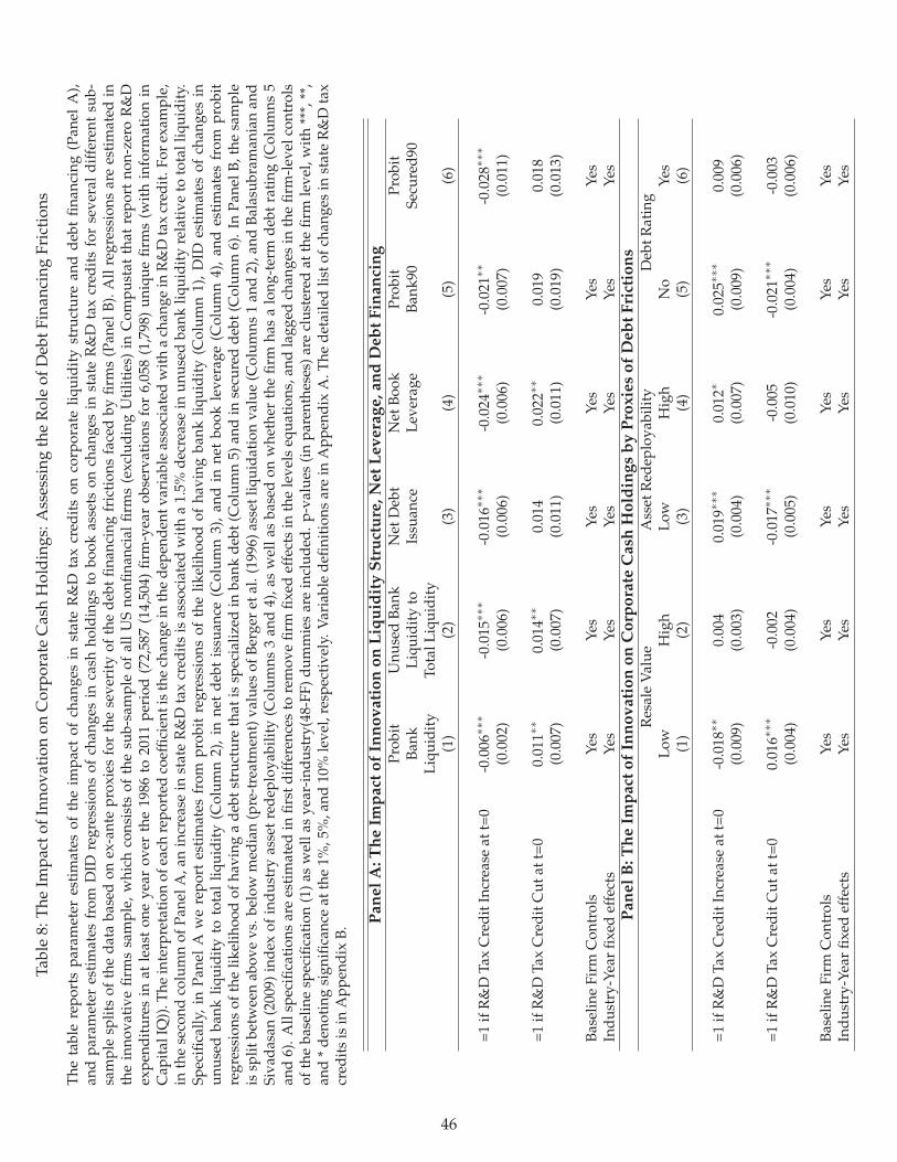
Tabl

e8:

The

Impa

ctof

Inno

vati

onon

Cor

pora

teC

ash

Hol

ding

s:A

sses

sing

the

Rol

eof

Deb

tFin

anci

ngFr

icti

ons

The

tabl

ere

port

spa

ram

eter

esti

mat

esof

the

impa

ctof

chan

ges

inst

ate

R&

Dta

xcr

edit

son

corp

orat

eliq

uidi

tyst

ruct

ure

and

debt

finan

cing

(Pan

elA

),an

dpa

ram

eter

esti

mat

esfr

omD

IDre

gres

sion

sof

chan

ges

inca

shho

ldin

gsto

book

asse

tson

chan

ges

inst

ate

R&

Dta

xcr

edit

sfo

rse

vera

ldi

ffer

ent

sub-

sam

ple

split

sof

the

data

base

don

ex-a

nte

prox

ies

for

the

seve

rity

ofth

ede

btfin

anci

ngfr

icti

ons

face

dby

firm

s(P

anel

B).A

llre

gres

sion

sar

ees

tim

ated

inth

ein

nova

tive

firm

ssa

mpl

e,w

hich

cons

ists

ofth

esu

b-sa

mpl

eof

all

US

nonfi

nanc

ial

firm

s(e

xclu

ding

Uti

litie

s)in

Com

pust

atth

atre

port

non-

zero

R&

Dex

pend

itur

esin

atle

ast

one

year

over

the

1986

to20

11pe

riod

(72,

587

(14,

504)

firm

-yea

rob

serv

atio

nsfo

r6,

058

(1,7

98)

uniq

uefir

ms

(wit

hin

form

atio

nin

Cap

ital

IQ))

.The

inte

rpre

tati

onof

each

repo

rted

coef

ficie

ntis

the

chan

gein

the

depe

nden

tvar

iabl

eas

soci

ated

wit

ha

chan

gein

R&

Dta

xcr

edit

.For

exam

ple,

inth

ese

cond

colu

mn

ofPa

nelA

,an

incr

ease

inst

ate

R&

Dta

xcr

edit

sis

asso

ciat

edw

ith

a1.

5%de

crea

sein

unus

edba

nkliq

uidi

tyre

lati

veto

tota

lliq

uidi

ty.

Spec

ifica

lly,

inPa

nel

Aw

ere

port

esti

mat

esfr

ompr

obit

regr

essi

ons

ofth

elik

elih

ood

ofha

ving

bank

liqui

dity

(Col

umn

1),

DID

esti

mat

esof

chan

ges

inun

used

bank

liqui

dity

toto

tal

liqui

dity

(Col

umn

2),

inne

tde

btis

suan

ce(C

olum

n3)

,an

din

net

book

leve

rage

(Col

umn

4),

and

esti

mat

esfr

ompr

obit

regr

essi

ons

ofth

elik

elih

ood

ofha

ving

ade

btst

ruct

ure

that

issp

ecia

lized

inba

nkde

bt(C

olum

n5)

and

inse

cure

dde

bt(C

olum

n6)

.In

Pane

lB,t

hesa

mpl

eis

split

betw

een

abov

evs

.bel

owm

edia

n(p

re-t

reat

men

t)va

lues

ofBe

rger

etal

.(19

96)a

sset

liqui

dati

onva

lue

(Col

umns

1an

d2)

,and

Bala

subr

aman

ian

and

Siva

dasa

n(2

009)

inde

xof

indu

stry

asse

tre

depl

oyab

ility

(Col

umns

3an

d4)

,as

wel

las

base

don

whe

ther

the

firm

has

alo

ng-t

erm

debt

rati

ng(C

olum

ns5

and

6).A

llsp

ecifi

cati

ons

are

esti

mat

edin

first

diff

eren

ces

tore

mov

efir

mfix

edef

fect

sin

the

leve

lseq

uati

ons,

and

lagg

edch

ange

sin

the

firm

-lev

elco

ntro

lsof

the

base

line

spec

ifica

tion

(1)a

sw

ella

sye

ar-i

ndus

try(

48-F

F)du

mm

ies

are

incl

uded

.p-

valu

es(i

npa

rent

hese

s)ar

ecl

uste

red

atth

efir

mle

vel,

wit

h**

*,**

,an

d*

deno

ting

sign

ifica

nce

atth

e1%

,5%

,and

10%

leve

l,re

spec

tive

ly.V

aria

ble

defin

itio

nsar

ein

App

endi

xA

.The

deta

iled

listo

fcha

nges

inst

ate

R&

Dta

xcr

edit

sis

inA

ppen

dix

B.

Pan

el

A:T

he

Imp

act

of

Inn

ov

ati

on

on

Liq

uid

ity

Str

uct

ure

,N

et

Lev

era

ge,an

dD

eb

tF

inan

cin

gPr

obit

Unu

sed

Bank

Net

Deb

tN

etBo

okPr

obit

Prob

itBa

nkLi

quid

ity

toIs

suan

ceLe

vera

geBa

nk90

Secu

red9

0Li

quid

ity

Tota

lLiq

uidi

ty(1

)(2

)(3

)(4

)(5

)(6

)

=1if

R&

DTa

xC

redi

tInc

reas

eat

t=0

-0.0

06∗∗∗

-0.0

15∗∗∗

-0.0

16∗∗∗

-0.0

24∗∗∗

-0.0

21∗∗

-0.0

28∗∗∗

(0.0

02)

(0.0

06)

(0.0

06)

(0.0

06)

(0.0

07)

(0.0

11)

=1if

R&

DTa

xC

redi

tCut

att=

00.

011∗∗

0.01

4∗∗

0.01

40.

022∗∗

0.01

90.

018

(0.0

07)

(0.0

07)

(0.0

11)

(0.0

11)

(0.0

19)

(0.0

13)

Base

line

Firm

Con

trol

sYe

sYe

sYe

sYe

sYe

sYe

sIn

dust

ry-Y

ear

fixed

effe

cts

Yes

Yes

Yes

Yes

Yes

Yes

Pan

el

B:T

he

Imp

act

of

Inn

ov

ati

on

on

Co

rpo

rate

Cash

Ho

ldin

gs

by

Pro

xie

so

fD

eb

tF

rict

ion

sR

esal

eV

alue

Ass

etR

edep

loya

bilit

yD

ebtR

atin

gLo

wH

igh

Low

Hig

hN

oYe

s(1

)(2

)(3

)(4

)(5

)(6

)

=1if

R&

DTa

xC

redi

tInc

reas

eat

t=0

-0.0

18∗∗

0.00

40.

019∗∗∗

0.01

2∗0.

025∗∗∗

0.00

9(0

.009

)(0

.003

)(0

.004

)(0

.007

)(0

.009

)(0

.006

)

=1if

R&

DTa

xC

redi

tCut

att=

00.

016∗∗∗

-0.0

02-0

.017∗∗∗

-0.0

05-0

.021∗∗∗

-0.0

03(0

.004

)(0

.004

)(0

.005

)(0

.010

)(0

.004

)(0

.006

)

Base

line

Firm

Con

trol

sYe

sYe

sYe

sYe

sYe

sYe

sIn

dust

ry-Y

ear

fixed

effe

cts

Yes

Yes

Yes

Yes

Yes

Yes

46

Tabl

e9:

The

Impa

ctof

Inno

vati

onon

Cor

pora

teC

ash

Hol

ding

s:A

sses

sing

the

Rol

eof

Equi

tyFi

nanc

ing

Fric

tion

s

The

tabl

ere

port

spa

ram

eter

esti

mat

esof

the

impa

ctof

chan

ges

inst

ate

R&

Dta

xcr

edit

son

equi

tyfin

anci

ng(P

anel

A),

and

para

met

eres

tim

ates

from

DID

regr

essi

ons

ofch

ange

sin

cash

hold

ings

tobo

okas

sets

onch

ange

sin

stat

eR

&D

tax

cred

its

for

seve

rald

iffer

ents

ub-s

ampl

esp

lits

ofth

eda

taba

sed

onex

-ant

epr

oxie

sfo

rth

ese

veri

tyof

the

equi

tyfin

anci

ngfr

icti

ons

face

dby

firm

s(P

anel

B).A

llre

gres

sion

sar

ees

tim

ated

inth

ein

nova

tive

firm

ssa

mpl

e,w

hich

cons

ists

ofth

esu

b-sa

mpl

eof

allU

Sno

nfina

ncia

lfirm

s(e

xclu

ding

Uti

litie

s)in

Com

pust

atth

atre

port

non-

zero

R&

Dex

pend

itur

esin

atle

asto

neye

arov

erth

e19

86to

2011

peri

od(7

2,58

7fir

m-y

ear

obse

rvat

ions

for

6,05

8un

ique

firm

s).T

hein

terp

reta

tion

ofea

chre

port

edco

effic

ient

isth

ech

ange

inth

ede

pend

entv

aria

ble

asso

ciat

edw

ith

ach

ange

inR

&D

tax

cred

it.

For

exam

ple,

inth

eth

ird

colu

mn

ofPa

nel

A,a

nin

crea

sein

stat

eR

&D

tax

cred

its

isas

soci

ated

wit

ha

3.6%

incr

ease

inca

shre

lati

veto

book

equi

ty.

Spec

ifica

lly,i

nPa

nel

Aw

ere

port

DID

esti

mat

esof

chan

ges

inne

teq

uity

issu

ance

(Col

umn

1)an

dca

shto

book

equi

tyra

tio

(Col

umn

3),a

ndes

tim

ates

from

prob

itre

gres

sion

sof

the

likel

ihoo

dof

ase

cond

ary

equi

tyis

sue

(SEO

)(C

olum

n2)

.In

Pane

lB,t

hesa

mpl

eis

split

betw

een

abov

evs

.be

low

med

ian

(pre

-tre

atm

ent)

valu

esof

the

tota

ldol

lar

volu

me

ofSE

Os

ina

firm

’s(4

8-FF

)in

dust

ryin

any

give

nye

ar(C

olum

ns1

and

2),t

heav

erag

e(0

,+1)

cum

ulat

ive

abno

rmal

retu

rn(C

AR

)ofS

EOs

anno

unce

men

tsin

afir

m’s

(48-

FF)i

ndus

try

inan

ygi

ven

year

(Col

umns

3an

d4)

,and

the

stan

dard

devi

atio

n(d

ispe

rsio

n)of

anal

ysts

’EPS

fore

cast

sfr

omIB

ES(C

olum

ns5

and

6).

All

spec

ifica

tion

sar

ees

tim

ated

infir

stdi

ffer

ence

sto

rem

ove

firm

fixed

effe

cts

inth

ele

vels

equa

tion

s,an

dla

gged

chan

ges

inth

efir

m-l

evel

cont

rols

ofth

eba

selin

esp

ecifi

cati

on(1

)as

wel

las

year

-ind

ustr

y(48

-FF)

dum

mie

sar

ein

clud

ed.

p-va

lues

(in

pare

nthe

ses)

are

clus

tere

dat

the

firm

leve

l,w

ith

***,

**,a

nd*

deno

ting

sign

ifica

nce

atth

e1%

,5%

,and

10%

leve

l,re

spec

tive

ly.

Var

iabl

ede

finit

ions

are

inA

ppen

dix

A.T

hede

taile

dlis

tofc

hang

esin

stat

eR

&D

tax

cred

its

isin

App

endi

xB.

Pan

el

A:T

he

Imp

act

of

Inn

ov

ati

on

on

Eq

uit

yF

inan

cin

gN

etEq

uity

Issu

ance

Prob

itEq

uity

Issu

ance

Cas

h/Bo

okEq

uity

(1)

(2)

(3)

=1if

R&

DTa

xC

redi

tInc

reas

eat

t=0

0.02

3***

0.04

1***

0.03

6***

(0.0

07)

(0.0

07)

(0.0

06)

=1if

R&

DTa

xC

redi

tCut

att=

0-0

.015

-0.0

27*

-0.0

32**

(0.0

11)

(0.0

14)

(0.0

16)

Base

line

Firm

Con

trol

sYe

sYe

sYe

sIn

dust

ry-Y

ear

fixed

effe

cts

Yes

Yes

Yes

Pan

el

B:T

he

Imp

act

of

Inn

ov

ati

on

on

Co

rpo

rate

Cash

Ho

ldin

gs

by

Pro

xie

so

fE

qu

ity

Fri

ctio

ns

SEO

Volu

me

SEO

Cos

tsA

naly

stFo

reca

stD

ispe

rsio

nLo

wH

igh

Low

Hig

hLo

wH

igh

(1)

(2)

(3)

(4)

(5)

(6)

=1if

R&

DTa

xC

redi

tInc

reas

eat

t=0

0.02

4***

0.01

00.

001

0.02

0***

0.00

90.

019*

*(0

.004

)(0

.016

)(0

.023

)(0

.005

)(0

.006

)(0

.008

)

=1if

R&

DTa

xC

redi

tCut

att=

0-0

.021

***

-0.0

09-0

.009

-0.0

29**

*-0

.002

-0.0

23**

(0.0

03)

(0.0

15)

(0.0

20)

(0.0

09)

(0.0

07)

(0.0

11)

Base

line

Firm

Con

trol

sYe

sYe

sYe

sYe

sYe

sYe

sIn

dust

ry-Y

ear

fixed

effe

cts

Yes

Yes

Yes

Yes

Yes

Yes

47

Tabl

e10

:The

Impa

ctof

Inno

vati

onon

Cor

pora

teC

ash

Hol

ding

s:A

sses

sing

the

Rol

eof

Age

ncy,

Rep

atri

atio

n,an

dIn

dust

ryC

ompe

titi

on

The

tabl

ere

port

spa

ram

eter

esti

mat

esfr

omD

IDre

gres

sion

sof

chan

ges

inca

shho

ldin

gsto

book

asse

tson

chan

ges

inst

ate

R&

Dta

xcr

edit

sfo

rse

vera

ldi

ffer

ent

sub-

sam

ple

split

sof

the

data

base

don

ex-a

nte

prox

ies

for

repa

tria

tion

ince

ntiv

esan

dpr

oduc

tm

arke

tco

mpe

titi

on(P

anel

A),

asw

ell

asof

the

seve

rity

ofag

ency

fric

tion

sfa

ced

byth

efir

m(P

anel

B).A

llre

gres

sion

sar

ees

tim

ated

inth

ein

nova

tive

firm

ssa

mpl

e,w

hich

cons

ists

ofth

esu

b-sa

mpl

eof

all

US

nonfi

nanc

ialfi

rms

(exc

ludi

ngU

tilit

ies)

inC

ompu

stat

that

repo

rtno

n-ze

roR

&D

expe

ndit

ures

inat

leas

ton

eye

arov

erth

e19

86to

2011

peri

od(7

2,58

7fir

m-y

ear

obse

rvat

ions

for

6,05

8un

ique

firm

s).

The

inte

rpre

tati

onof

each

repo

rted

coef

ficie

ntis

the

chan

gein

the

depe

nden

tva

riab

leas

soci

ated

wit

ha

chan

gein

R&

Dta

xcr

edit

.Fo

rex

ampl

e,in

the

seco

ndco

lum

n,an

incr

ease

inst

ate

R&

Dta

xcr

edit

sis

asso

ciat

edw

ith

a1.

5%in

crea

sein

cash

rela

tive

tobo

okas

sets

.In

Pane

lA,t

hesa

mpl

eis

split

betw

een

abov

evs

.be

low

med

ian

(pre

-tre

atm

ent)

valu

esof

the

fore

ign

tax

burd

enm

easu

reof

Fole

y,H

artz

ell,

and

Titm

an(2

007)

(Col

umns

1an

d2)

,the

(48-

FF)i

ndus

try

Her

finda

hl-H

irsc

hman

Inde

x(H

HI)

ofsa

les

(Col

umns

5an

d6)

,and

base

don

whe

ther

the

firm

repo

rts

fore

ign

inco

me

ina

give

nye

ar(C

olum

ns3

and

4).I

nPa

nelB

,we

cons

ider

only

the

sub-

sam

ple

offir

ms

inre

lati

vely

conc

entr

ated

indu

stri

es(t

hose

wit

hab

ove-

med

ian

HH

I)an

dfu

rthe

rsp

litth

esa

mpl

ebe

twee

nab

ove

vs.

belo

wm

edia

n(p

re-t

reat

men

t)va

lues

ofbo

ard

size

(Col

umns

1an

d2)

,bo

ard

inde

pend

ence

(Col

umns

5an

d6)

,and

base

don

whe

ther

the

firm

has

acl

assi

fied

boar

dof

dire

ctor

s(C

olum

ns3

and

4).

All

spec

ifica

tion

sar

ees

tim

ated

infir

stdi

ffer

ence

sto

rem

ove

firm

fixed

effe

cts

inth

ele

vels

equa

tion

s,an

dla

gged

chan

ges

inth

efir

m-l

evel

cont

rols

ofth

eba

selin

esp

ecifi

cati

on(1

)as

wel

las

year

-ind

ustr

y(48

-FF)

dum

mie

sar

ein

clud

ed.p

-val

ues

(in

pare

nthe

ses)

are

clus

tere

dat

the

firm

leve

l,w

ith

***,

**,a

nd*

deno

ting

sign

ifica

nce

atth

e1%

,5%

,an

d10

%le

vel,

resp

ecti

vely

.Var

iabl

ede

finit

ions

are

inA

ppen

dix

A.T

hede

taile

dlis

tofc

hang

esin

stat

eR

&D

tax

cred

its

isin

App

endi

xB.

Pan

el

A:T

he

Imp

act

of

Inn

ov

ati

on

on

Co

rpo

rate

Cash

Ho

ldin

gs

by

Pro

xie

so

fR

ep

atr

iati

on

&P

rod

uct

Mark

et

Co

mp

eti

tio

nFo

reig

nTa

xBu

rden

Fore

ign

Inco

me>

0In

dust

ryH

HI

Hig

hLo

wYe

sN

oLo

wH

igh

(1)

(2)

(3)

(4)

(5)

(6)

=1if

R&

DTa

xC

redi

tInc

reas

eat

t=0

-0.0

070.

015*

**0.

007*

0.02

4***

0.01

7***

0.01

3(0

.007

)(0

.005

)(0

.004

)(0

.005

)(0

.003

)(0

.009

)

=1if

R&

DTa

xC

redi

tCut

att=

0-0

.005

-0.0

14*

-0.0

09-0

.023

*-0

.017

***

-0.0

06(0

.011

)(0

.008

)(0

.006

)(0

.012

)(0

.006

)(0

.008

)

Base

line

Firm

Con

trol

sYe

sYe

sYe

sYe

sYe

sYe

sIn

dust

ry-Y

ear

fixed

effe

cts

Yes

Yes

Yes

Yes

Yes

Yes

Pan

el

B:T

he

Imp

act

of

Inn

ov

ati

on

on

Co

rpo

rate

Cash

Ho

ldin

gs

by

Pro

xie

so

fA

gen

cy&

Go

vern

an

ceF

rict

ion

sBo

ard

Size

inC

lass

ified

Boar

din

Boar

dIn

depe

nden

ce(%

Out

side

Hig

hH

HII

ndus

trie

sH

igh

HH

IInd

ustr

ies

Dir

ecto

rs)i

nH

igh

HH

IInd

ustr

ies

Low

Hig

hN

oYe

sH

igh

Low

(1)

(2)

(3)

(4)

(5)

(6)

=1if

R&

DTa

xC

redi

tInc

reas

eat

t=0

0.00

50.

013*

**0.

007

0.01

8**

0.01

0**

0.01

5***

(0.0

05)

(0.0

05)

(0.0

07)

(0.0

07)

(0.0

04)

(0.0

05)

=1if

R&

DTa

xC

redi

tCut

att=

0-0

.007

-0.0

17*

-0.0

08-0

.017

*-0

.007

-0.0

20*

(0.0

07)

(0.0

10)

(0.0

08)

(0.0

10)

(0.0

07)

(0.0

12)

Base

line

Firm

Con

trol

sYe

sYe

sYe

sYe

sYe

sYe

sIn

dust

ry-Y

ear

fixed

effe

cts

Yes

Yes

Yes

Yes

Yes

Yes

48

Figure 1: History of Changes in State R&D Tax Credits

This figure shows the pattern of changes in all state R&D tax credits (subsequent to their introduction) betweentax years 1987 and 2011. The left column shows the pattern of cuts in state R&D tax credits, and the rightcolumn shows the pattern of increases in state R&D tax credits. We hand-collected this information for allU.S. states using a variety of sources. The State Tax Handbook (various years) and Wilson (2009) provided thestarting point to get a summary list of R&D tax credits available in any given state at a particular point in time.We then cross-checked this information by verifying the passage of state tax bills and obtaining information onthe year when a given tax credit becomes effective by performing keyword searches in Lexis-Nexis (State Net)and online searches of state code legislation and tax forms on the states’ Department of Revenue websites.

49

Figure 2: Annual Changes in Cash Holdings Around Changes in State R&D Tax Credits

This figure plots average annual within-firm changes in cash to book asset ratios for each year in a five-yearwindow around the year when a state increases (Panel A) or cuts (Panel B) its R&D tax credit (t=0). Plottedchanges are in excess of contemporaneous cash changes in the firm’s 48-FF industry, to remove the influenceof time-varying changes in industry conditions, and of predicted changes based on pre-treatment cash levels,to control for partial adjustment of cash. The solid, red bars are for treated firms and the dotted, blue bars arefor controls, and the difference between the two bars in a given year – i.e., the difference-in-difference estimate– is displayed for t=0 (with its respective (two-sided) t-test of significance using standard errors clustered atthe firm level, with ***, **, and * denoting significance at the 1%, 5%, and 10% level, respectively).

Panel A: Increases in State R&D Tax Credits

Panel B: Cuts in State R&D Tax Credits

50