Why are Income Distributions Different?: A Comparison of Brazil and the United States

François Bourguignon, Francisco H. G. Ferreira and Phillippe G. Leite1

Keywords: Inequality, Distribution, Micro-simulations

JEL Classification Codes: C15, D31, J22

Abstract: Although most people agree that differences in income distributions across countries matter, little is known about what determines them. This paper develops a micro-econometric method to account for differences across distributions of household income. Going beyond the determination of earnings in labor markets, we also estimate statistical models for occupational choice and for the conditional distributions of education, fertility and non-labor incomes. We use combinations of estimated parameters from these models to simulate counterfactual income distributions. This allows us to decompose differences between functionals of two income distributions (such as inequality or poverty measures) into shares due to differences in the structure of labor market returns (price effects); differences in the occupational structure; and differences in the underlying distribution of assets (endowment effects). We apply the method to the differences between the income distributions of the US and Brazil, and find that most of Brazil's excess income inequality relative to the United States is due to underlying inequalities in the distribution of two key endowments: access to education and to sources of non-labor income, mainly pensions. Steeper returns to education in Brazil also contribute, but are of secondary importance. Differences in occupational structures are immaterial.

1 Bourguignon is with DELTA, Paris, and the World Bank. Ferreira and Leite are at the Pontifícia Universidade Católica do Rio de Janeiro and the World Bank. We thank David Lam, Dean Jolliffe, Klara Sabirianova and seminar participants at PUC-Rio, IBMEC-Rio, the University of Michigan, the World Bank and DELTA for helpful comments. The opinions expressed here are those of the authors and do not necessarily reflect those of the World Bank, its Executive Directors or the countries they represent.

2

1. Introduction

The distribution of personal welfare varies enormously across countries. Gini coefficients

for distributions of household income per capita, for instance, range from 0.20 in the

Slovak Republic to 0.63 in Sierra Leone (World Bank, 2002) and similar international

variation can be found for most alternative measures of inequality. This international

variation is much greater than the variation ever encountered in any single time-series of

inequality measures for any given country – including both developed countries with long

histories of reliable data, like the UK or the US (see e.g. Kuznets, 1955), and transition

economies with dramatic recent distributional changes (see e.g. Milanovic, 1998).

One would think, then, that there ought to be considerable interest in understanding why

income distributions vary so much across countries. After all, different inequality levels or

poverty rates are likely to matter both for the current welfare levels of a society and for its

long-term development and growth prospects. More unequal societies may create different

institutions, with possibly persistent and deleterious effects on the development process

(Engerman and Sokoloff, 1997). The outcomes of similar political processes may, because

of different income distributions, lead to different social contracts, including different

choices about taxation and redistribution (Bénabou, 2000; Ferreira, 2001). Different income

distributions may lead to different patterns of occupational choice; with consequently

different labor market outcomes, which have been hypothesized to lead to multiple

equilibria in the long-run (Banerjee and Newman, 1993). In fact, economic thinking about

growth and development since the early 1990s has, as Anthony Atkinson (1997) put it,

brought “income distribution in from the cold”, and back into the fairly central position it

used to occupy for classical economists like David Ricardo.

Yet, surprisingly little is known about how and why income distributions actually differ

across countries.2 Is it because the underlying distributions of wealth differ greatly, perhaps

2 There has been a much greater concern with testing the proposition that inequality is bad for growth (e.g. Forbes, 2000). That literature has not been particularly conclusive (Banerjee and Duflo, 2000). But our concern here is with a basic empirical understanding of the nature – rather than of the effects - of distributional differences.

3

for historical reasons (Engerman et. al., 1998)? Or is it because returns to education are

higher in one country than in the other (e.g. Blau and Khan, 1996)? What is the role of

differences in labor market institutions (e.g. Calmfors and Driffill, 1988; DiNardo et.al.,

1996)? Do different fertility rates and family structures play a role? And if, as is likely,

differences in income distributions reflect all of these (and possibly other) factors, in what

manner and to what extent does each one contribute?

Applied research on differences across income distributions has not been as abundant as

one might expect.3 Increasingly, this seems to have less to do with lack of data and more to

do with inadequate methodological tools. Through initiatives like the Luxembourg Income

Study and the WIDER World Income Inequality Database, the availability of high-quality

household-level data is growing. Methodologically, however, those seeking an

understanding of why distributions are so different - and reluctant to rely exclusively on

cross-country regressions with inequality measures as dependent variables - have often had

to resort to comparing Theil decompositions across countries.4 We will argue below that,

while these can be informative, their ability to shed light on the determinants of differences

across distributions is inherently limited.

In contrast, much more substantial progress has been made in our ability to understand

differences in wage (or earnings) distributions. Some of this work - such as Almeida dos

Reis and Paes de Barros (1991), Juhn, Murphy and Pierce (1993), Blau and Khan (1996)

and Machado and Mata (2001) - draws on variants of a decomposition technique based on

simulating counterfactual distributions by combining data on individual characteristics (X)

from one distribution, with estimated parameters (β) from another, which is due originally

to Oaxaca (1973) and Blinder (1973).5 Another strand, which includes DiNardo, Fortin and

3 As noted, theoretical models of why income distributions might differ across countries have been more abundant. Banerjee and Newman (1993) and Bénabou (2000) are two well-known examples. See Aghion et. al. (1999) for a survey. 4 Theil decompositions are also known as decompositions of Generalized Entropy inequality measures by population subgroups. They were developed independently by Bourguignon (1979), Cowell (1980) and Shorrocks (1980). 5 Some of these studies - like Juhn, Murphy and Pierce (1993) and Machado and Mata (2001) - decompose changes in the wage distribution of a single country, over time. Others, like Almeida dos Reis and Paes de Barros (for metropolitan areas within Brazil) and Blau and Khan (for ten industrialized countries) decompose

4

Lemieux (1996) and Donald, Green and Paarsch (2000), is based on alternative semi-

parametric approaches. DiNardo et. al. (1996) use weighted kernel density estimators -

instead of regression coefficients - to generate counterfactual density functions that

combine population attributes (or labor market institutions) from one period, with the

structure of returns from another. Donald et. al. (2000) adapt hazard-function estimators

from the spell-duration literature to develop density-function estimators, and use these to

construct counterfactual density and distribution functions (comparing the US and

Canada).6

These approaches have been very fruitful, but they have not yet been generalized from

wage distributions to those of household incomes, largely because the latter involve

additional complexities.7 The distribution of wages is usually defined over those currently

employed. Taking the characteristics of these workers as given, earnings determination can

be reasonably well understood by estimating returns to those characteristics in the labor

market, through a Mincerian earnings equation: iii Xy εβ += . Most of the aforementioned

recent literature on differences in wage inequality is based on simulating counterfactual

distributions on the basis of equations such as this, and many further restrict their samples

to include prime-age, full-time male workers only. In addition, some authors are quite clear

that they are interested in wages primarily as indicators of the price of labor, rather than as

measures of welfare (e.g. Juhn, Murphy and Pierce, 1993). While this is perfectly adequate

for their purposes, it does mean that these are not studies about international differences in

the distribution of welfare. The latter, which would be better proxied by distributions of

household per capita incomes or expenditures, are our focus here.

differences across wage distributions for different spatial units. For a less well-known but also pioneering piece, see Langoni (1973). 6 The distinction between "parametric" and "semi-parametric" methods is not terribly sharp. DiNardo et. al. (1996) use a probit model to estimate one of their conditional reweighing functions. Donald et. al. (2000) rely entirely on maximum likelihood estimates of parameters in a proportional-hazards model, and what is non-parametric about their method is a fine double-partitioning of the income space, allowing for considerable flexibility in both the estimation of the baseline hazard function, and in the manner in which it is shifted by the proportional-hazards estimates. Conversely, in the present paper, which follows a predominantly parametric route, some non-parametric reweighing of joint distribution functions is also used (see below). These techniques are often better thought of as complements, rather than substitutes. 7 From a conceptual point of view this should matter, since it is the distribution of household incomes, rather than that of individual wages, which is more likely to affect voting behavior or the educational credit available to the family.

5

Naturally, the distribution of household incomes does depend on the characteristics of the

employed members of the household and on the rates of return to them, and we will thus

draw on earnings models too. But it also depends on their participation and occupational

decisions, as well as on choices concerning the size and composition of the family. In

addition, changes in some personal characteristics - such as education - affect household

incomes through more than one channel. Suppose we ask what the effect of “importing” the

US distribution of education to Brazil might be on the Brazilian distributions of earnings

and incomes. Whereas for earnings it might very well suffice to simply replace the

Brazilian vector of years of schooling in the X matrix with the relevant US values, the

distribution of household incomes will also be affected through changes in participation and

fertility behavior. This greater complexity of the determinants of household income

distributions seems to have prevented counterfactual simulation techniques from being

applied to them, thus depriving those interested in understanding cross-country differences

in the distribution of welfare from the powerful insights they can deliver.

Nevertheless, a more general version of the Oaxaca-Blinder idea – of simulating

counterfactual distributions on the basis of combining models estimated for different real

distributions - can fruitfully be applied to household incomes. What is required is an

expansion of the set of models to be estimated, to include labor market participation,

fertility behavior and educational choices. In this paper, we first propose a general

statement of statistical decompositions applied to household income distributions; and then

suggest a specific model of household income determination that enables us to implement

the decomposition empirically. In particular, we investigate the comparative roles of three

factors: the distribution of population characteristics (or endowments); the structure of

returns to these endowments, and the occupational structure of the population. We apply

the method to an understanding of the differences between the income distributions in

Brazil and the United States – the two most populous countries in the Western hemisphere,

both of which are very unequal for their per capita GDP levels.

6

The paper is organized as follows. Section 2 presents the data and some preliminary

description of income distributions in the two countries. Doing so also motivates the need

for better tools to understand the large differences between them. Section 3 contains a

general statement of statistical decomposition analysis, which encompasses all variants

currently in use as special cases. Section 4 proposes a specific model of household income

determination and describes the estimation and simulation procedures needed for the

decomposition. The results are discussed in section 5, and section 6 concludes.

2. Income Distribution in Brazil and the United States: preliminaries.

This section compares the distributions of household income in the two largest countries in

the Western Hemisphere: the United States and Brazil. This choice of countries is not

accidental: since we are, in some sense, interested in understanding inequality, we want

places with lots of it. Decomposing differences between the distributions of Sweden and

Slovakia would not have been a good first test of the approach. Secondly, we also want

countries which are at different stages in development – and in particular which have truly

different distributions of educational attainments – since this difference is a central

candidate for explaining income differences. This makes a comparison between a large and

unequal developing country with relatively low levels of education, and a large and

relatively unequal industrial nation with very high levels of education, particularly

interesting.8

The comparisons are based on the original household-level data sets: the Pesquisa Nacional

por Amostra de Domicílios (PNAD) 1999 is used for Brazil, and the Annual Demographic

Survey in the March Supplement to the Current Population Survey (CPS/ADS) 2000, for

the United States. The PNAD income data refers to the month of September 1999. As

always with the March Supplement of the CPS/ADS, total personal income data refers to

the preceding calendar year, 1999, so that both surveys refer to the same year. The sizes of

8 Our emphasis here is purely comparative. We make no attempt to present a detailed analysis of inequality or poverty in each of these countries. There is a large literature on the subject for both countries. On Brazil, see Henriques (2000) for a recent compilation. For earlier studies comparing the Brazilian and US earnings distributions, see Lam and Levison (1992) and Sacconato and Menezes-Filho (2001).

7

the samples actually used are as follows: the CPS/ADS 2000 contained 50,982 households

(133,649 individuals), and the PNAD 1999 contained 80,972 households (294,244

individuals).

We use income data, rather than data on consumption expenditures, because the

decompositions described in the remainder of the paper rely in part on the determination of

earnings.9 For Brazil, the income variable used was monthly total household income per

capita, available in the surveys as a constructed variable from the disaggregated income

questionnaire. In the US, the variable used was the sum (across individuals in the

household) of annual total personal income and other incomes, excluding disability

benefits, educational assistance and child support, divided by 12.10 Both income definitions

are before tax, but include transfers. While total annual incomes are not top-coded in the

CPS/ADS, some of their components might be. The US Census Bureau warns that weekly

earnings, in particular, are "subject to top-coding at U$1923", so as to censor the

distribution of annual earnings from the main job at U$100,000. Inspection of our sample

revealed, however, that 2.1% (2.5%) of observations had reported weekly (annual) earnings

above those value. The maximum reported weekly value was U$2884. We therefore did not

correct for top-coding in the US. Incomes are not top-coded in Brazil either.

As always, there are reasons to suspect that incomes may be measured with some error. In

the case of Brazil, the problem is particularly severe in rural areas, to the extent that the

usefulness of any estimate based on rural income data is thrown into doubt.11 For this

reason, we prefer to confine our attention to Brazil’s urban areas only.12 Care is taken to

ensure that the distributions used are as comparable as possible, and this requires that we

9 And also because consumption data for Brazil is either very old (ENDEF, 1975) or incomplete in geographical coverage (POF, 1996; PPV, 1996). 10 These income sources were excluded from the analysis because non-retirement public transfers are proportionately much more important in the US than in Brazil, and their allocation follows rules which are not modelled in our approach. When they were included, the residual term of the decomposition was slightly larger, but all of our conclusions remained qualitatively valid. 11 For evidence on the weaknesses of income data for rural Brazil, see Ferreira, Lanjouw and Neri (2000) and Elbers, Lanjouw, Lanjouw and Leite (2001). 12 For the US, since the CPS/ADS does not disaggregate non-metropolitan areas into urban and rural, and the former dominate, we included both metropolitan and non-metropolitan areas.

8

work with data unadjusted for misreporting, imputed rents, or for regional price level

differences within countries. 13

With 168 million inhabitants in 1999, Brazil’s population was approximately 60% that of

the United States (273 million). In the same year, Brazil’s per capita GDP from the

National Accounts was 20% that of the US. Mean per capita income as measured by the

household surveys was slightly less, at 17%. Brazil's urban inequality, on the other hand, is

much higher. Its Gini coefficient of 0.569 was twelve and a half percentage points higher

than that of the US. Brazil’s Theil-T (or E(1) index) was 0.644, whereas the US’s was

0.349. Bourguignon et. al. (2002) show that this pattern is robust to (considerable) variation

in the degree of economies of scale in household consumption, allowed for through the

Buhmann et. al. (1988) parameter. It is also robust to the choice of inequality measures,

since the Lorenz curve for the US lies everywhere strictly above that for urban Brazil,

indicating that inequality is unambiguously lower in the former (Atkinson, 1970).

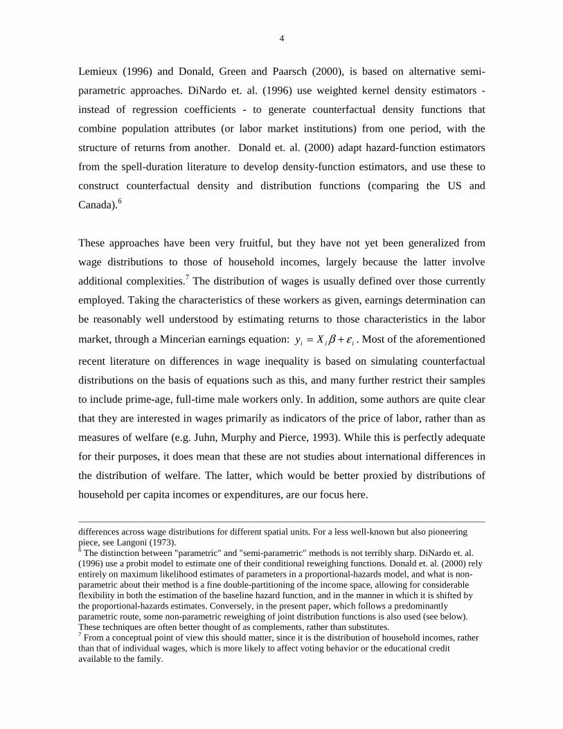
But income distributions do not differ only with respect to their fist two moments. One

advantage of the approach we propose is exactly that it allows us to visualize the impacts of

different factors on different parts of the distribution in an entirely disaggregated way. As a

preliminary, then, it is useful to see that the income distributions for urban Brazil and the

United States in 1999 did not differ only in mean and inequality. Figure 1 below plots

kernel estimates of the (mean normalized) density functions for the distribution of (the

logarithm of) household per capita income in both countries. The differences in skewness

and kurtosis, for example, are immediately obvious, with Brazil’s distribution being more

skewed to the left and having thicker tails.

We are not aware of empirical methods for comparing household income distributions

which can account for these differences. As an example of a common approach, Table 1

reports on standard decompositions of E(0), E(1) and E(2) by population subgroups14,

computing the RB statistic developed by Cowell and Jenkins (1995). This statistic is an

13 Both datasets are well-known in their respective countries. For more detailed information about the CPS/ADS, go to www.census.gov. Information on the PNAD is available from www.ibge.gov.br. 14 See Bourguignon (1979), Cowell (1980) and Shorrocks (1980).

9

indicator of the relative importance of each attribute used to partition the population, in the

process of "accounting for" the inequality. The idea is that the larger the share of dispersion

which is between groups defined by some attribute - rather than within those groups - the

more likely it is that something about the distribution of or returns to that attribute are

causally related to the observed inequality. The attributes to be used include education of

the household head; his or her age; his or her race or ethnic group; his or her gender; as

well as the location of the household (both regional and rural/urban) and its size or type.

Figure 1: Kernel Density Estimates of the Distributions of Household Incomes,Brazil and the United States

0.0

0.1

0.2

0.3

0.4

0.5

0.6

0 2 4 6 8 10 12Log income

Den

sity

Brazil

USA

Source: PNAD/IBGE 1999, CPS/ADS 2000 and author's calculationNote: Gaussian Kernel Estimates (with optimal window width) of the density functions for the distributions of the logarithms of household per capita incomes. The distribution were scaled so as to have the Brazilian mean. Brazil is urban area only. Incomes were converted to US dollar at PPP exchange rates (see Appendix).

The results are suggestive. In Brazil, education of the head is clearly the most important

partitioning characteristic, followed by race and household type. In the US, household type

dominates, with education a surprisingly low second, and age of head third. Education

clearly accounts for more inequality in Brazil than in the US, although these

decompositions can not tell us whether this is due predominantly to different returns or

different endowments of education – i.e. a different distribution of the population across

educational levels. Strikingly little of the overall US inequality is between different regions

of the country, reinforcing the widespread perception of a well-integrated economy. In

contrast, almost 10% of Brazil’s Theil-L is accounted for by the regional partition.15

15 The regional breakdowns used in this decomposition were standard for each country. Brazil was divided up into five regions: North, Northeast, Centre-West, Southeast and South, while the US was broken down into four regions: Northeast, Midwest, South and West.

10

Finally, it is interesting to note that inequality between households headed by people of

different races - which one might have expect to be prominent in the US - is five times

larger in Brazil.

Although this is a useful preliminary exercise, there are at least three reasons why one

would wish to go further. First, none of these decompositions control for any of the others:

some of the inequality between regions in Brazil is also between individuals with different

races – given that racial compositions varies considerably across regions - and there is no

way of telling how much. Second, the decompositions are of scalar measures, and therefore

“waste” information on how the entire distributions differ (along their support). Although

some information can be recovered from knowledge of the different sensitivities of each

measure, this is at best a hazardous and imprecise route. Finally, even to the extent that one

is prepared to treat inequality between subgroups defined by age or education, say, as being

driven by those attributes – rather than by correlates – the share of total inequality

attributed to that partition tells us nothing of whether it is the distribution of the

characteristic (or asset), or the structure of its returns that matters. In the next section, we

propose an alternative approach, which suffers from none of these shortcomings.

3. A General Statement of Statistical Decomposition Analysis.

In order to understand the differences between two distributions of household incomes,

fA(y) and fB(y), it seems natural to depart from the joint distributions ϕC(y, T), where T is a

vector of observed household characteristics which affect incomes - such as family size, the

age, gender, race, education and occupation of each individual member of the household,

etc.. The superscript C (= A, B) denotes the country. Because a number (but not all) of the

characteristics in T clearly depend on others (e.g. family size, via the number of children,

will vary with the age and education of the parents), it will prove helpful to partition T =

[V, W] where, for any given household h in C, each element of Vh may be thought of as

logically depending on Wh, and possibly on some other elements of Vh, but Wh is to be

considered as fully exogenous to the household.

11

The distribution of household incomes, fC(y), is of course the marginal distribution of the

joint distribution ϕC(y, T) : ( )∫∫∫∫ ⋅⋅= dTTyyf CC ,)( ϕ . It can therefore be rewritten as

( ) ( ) ( )dVdWWVWVygyf CCC ,, ζ∫∫∫∫ ⋅⋅= , where gC(y | V,W) denotes the distribution of y

conditional on V and W, and ζC(V, W) is the joint distribution on all elements of T in

country C. Given the distinction made above between the “semi-exogenous”16 household

characteristics V and the “truly exogenous” characteristics W, this can be further rewritten

as:

(1) ( ) ( ) ( ) ( ) ( ) ( )dVdWWWvhWVvhWVvhWVygyf CCCCCC ψυυ...,,, 2,122111 −−∫∫∫∫ ⋅⋅=

In (1), the joint distribution of all elements of T = [V, W] has been replaced by the product

of υ conditional distributions and the joint distribution of all elements in W, ψC(W). Each

conditional distribution hn is for an element of V, conditioning on the υ-n elements of V not

yet conditioned on, and on W. The order n = 1,…υ obviously does not matter for the

product of the conditional distributions. (1) is an identity, invariant in that ordering.

However, the order does matter for the definition of each individual conditional distribution

hn(vn|V-1,…,n, W), and therefore for the interpretation of each decomposition defined below.17

Once we have written the distributions of household incomes for countries C = A, B as in

(1), one could investigate how fB(y) differs from fA(y) by replacing some of the observed

conditional distributions in the ordered set kA = gA, hA by the corresponding conditional

distributions in the ordered set kB = gB, hB. Each such replacement generates a

counterfactual (ordered) set of conditional distributions ks, the dimension of which is υ+1,

(like kA and kB) whose elements are drawn either from kA or kB.18 It is now possible to

define a counterfactual distribution fsA→B(y; ks, ψA) as the marginal distribution that arises

16 This terminology is motivated by the fact that we do not pretend that our models of V should be interpreted causally, and make no claims to be endogenizing these variables in a behavioural sense. 17 Shorrocks (1999) proposes an algorithm based on the Shapley Value in order to calculate the correct "average" contribution of a particular hn( ) or of g( ), over the set of possible orderings, to the overall difference across the distributions. Rather than constructing these values in this paper, we present our results by showing a number of different orderings explicitly, in Section 5 below. 18 Formally, s is an ordered sequence of country superscripts, such as s = A, B, A, A, A, …, A.

12

from the integration of the product of the conditional distributions in ks and the joint

distribution function ψA(W), with respect to all elements of V and W. For example:

( ) ( ) ( ) ( ) ( ) ( )dVdWWWvhWVvhWVvhWVygyf AAABAsBA ψυυ...,,, 2,122111 −−→ ∫∫∫∫ ⋅⋅= . The

number of possible such counterfactual distributions is the number of possible permutations

in the set k.19

For each counterfactual distribution, it is possible to decompose the observed difference in

the income distributions for countries A and B as follows:

(2) ( ) ( ) ( ) ( )[ ] ( ) ( )[ ]yfyfyfyfyfyf sBAsAB −+−=−

where the first term on the right-hand side measures the “explanatory power” of

decomposition s, and the second term measures the “residual” of decomposition s.20 Since

these are differences in densities, they can be evaluated for all values of y. Furthermore, any

functional of a density function can be evaluated for fA, fB or fs, and similarly decomposed,

according to its own metric.

So, we have the same decomposition relationship as (2) for the cumulative distribution

( ) ( )∫=y

CC dxxfyF0

. Likewise, for the mean income of intervals between quantiles q-1 and

q (where there are Q intervals21): ( ) ( )( )

( )

∫−

− −

=qF

qF

CCq

C

C

dyyyfQ

y

1

1 1

1µ , we have:

(3) ( ) ( ) ( ) ( )[ ] ( ) ( )[ ]yyyyyy sq

Bq

Aq

sq

Aq

Bq µµµµµµ −+−=−

And we have analogous decompositions for any inequality measure I(f(y)) or poverty

measure P(f(y); z), where z is a suitable poverty line. In the applications discussed in

19 When we turn to the empirical implementation of these counterfactual distributions, we will see that is also possible, of course, to simulate replacing the joint distribution ψA(y) by a non-parametric approximation of ψB(y). Depending on how each specific conditional distribution is modelled, it is also possible to have more than one counterfactual distribution per element of k. These matters pertain more properly to a discussion of the empirical application of the approach, however, and we return to them later. 20 A decomposition is defined (by (2)) with respect to a unique counterfactual distribution s, and is thus also indexed by s.

13

Section 5, the results are presented exactly in this form: Table 3 contains inequality and

poverty measures, evaluated for fA(y), fB(y) and for a set of counterfactual distributions fs(y),

so that the reader can make his own subtractions. Figures 2-6 plot the differences in the

(log) mean income of “hundredths” (Q = 100), in a graphical representation of Equation

(3). In recognition of their parentage, we call these the Generalized Oaxaca-Blinder

decompositions.

4. The Decompositions in Practice: A Specific Model

The essence of the approach outlined above is to compare two actual income distributions,

by means of a sequence of “intermediate” counterfactual distributions. These are

constructed by replacing one or more of the underlying conditional distributions of A by

those imported from B. In practice, this requires generating statistical approximations to the

true conditional distributions. This may be done either parametrically - following the

tradition of Oaxaca (1973), Blinder (1973) and Almeida dos Reis and Paes de Barros

(1991) - or using non-parametric techniques – as in DiNardo, Fortin and Lemieux (1996).22

Because of the direct economic interpretations of the parameter estimates in our

approximated distributions, we find it convenient in this paper to follow (mainly) the

parametric route and approximate each of the true conditional distributions by a set of

standard econometric models, with pre-imposed functional forms.23

In particular, we will find it convenient to propose two (sets of) models:

(4) y = G (V, W, ε; Ω) and

(5) V = H (W, η; Φ),

where Ω and Φ are sets of parameters and ε and η stand for vectors of random variables,

with ε⊥V, W, and η⊥W, by construction. G and H have pre-imposed functional forms.

21 Or Q-1 quantiles. So, for instance, Q = 4 (10, 100) for quartiles (deciles, percentiles). 22 Although, as noted earlier, these authors too rely on parametric approximations to some conditional distributions, such as the probit for the conditional distribution of union status on individual characteristics. 23 This is an advantage of our approach vis-à-vis, for instance, the hazard-function estimators of Donald et. al. (2000), who "note that the estimates of the hazard function for wages, earnings or incomes are difficult to interpret" (p.616)

14

We can then write an approximation f*(y) to the true marginal distribution fC(y) in Equation

(1) as:

(1’) ( ) ( ) ( )( )

( )( )∫ ∫

=Ω =Φ

Ψ

=

yWVG

C

VWH

vyC dVdWWddyf;,, ,,

*

ε η

ηηπεεπ

where πy(ε) is the joint probability distribution function of the elements of ε and πv(η) is the

joint probability distribution function of the elements of η.

Just as an exact decomposition was defined by (2) for each true counterfactual distribution,

we can now define the (actually operational) decomposition s in terms of the approximated

distributions f *(y), as follows:

(2’) ( ) ( ) ( ) ( )[ ] ( ) ( )[ ] ( ) ( )[ ]yfyfyfyfyfyfyfyf sssBAsAB ** −+−+−=− .

Recall that a counterfactual distribution s is conceptually given by fsA→B(y; ks, ψA), and is

thus defined by (ψA and) the simulated sequence of conditional distributions ks, which

consists of some original distributions from A, and some imported from B. Analogously, an

approximated distribution ( )AsssBA yf ΨΦΩ→ ,,;* is defined with respect to (ψA and) the two

sets of simulated parameters Ωs and Φs, which consist of some original parameters from the

models estimated for country A, and some imported from the models estimated for country

B.

The last term in (2') gives the difference between the true and the approximated

counterfactual distributions. We therefore call it the approximation error and denote it by

RA. Clearly, how useful this decomposition methodology is in accounting for differences

between income distributions depends to some extent on the relative size of the

approximation error. The comparison between Brazil and the United States, discussed in

the next section, illustrates that it can be remarkably small.

Following from (1’), our statistical model of household incomes has three levels. The first

corresponds to model G (V, W, ε; Ω), which seeks to approximate the conditional

15

distribution of household incomes on observed characteristics: g (y| V,W). This level

generates estimates for the parameter set Ω, which we associate with the structure of

returns in the labor markets and with the determination of the occupational structure in the

economy. The second level corresponds to model H (W, η; Φ) which seeks to approximate

the conditional distributions hn (vn|V-1,…,n, W), for V =number of children in the household

(nch); years of schooling of individual i (Eih); and total household non-labor income (y0h)

In the third level, we investigate the effects of replacing ψA(W) with a (non-parametric)

estimate of ψB(W). This largely corresponds to the racial and demographic make-up of the

population.

First-level model G (V, W, ε; Ω) is given by equations (6-8) below. Household incomes are

an aggregation of individual earnings yhi, and of additional, unearned income such as

transfers or capital income, y0. Per capita household income for household h is given by:

(6)

+Ι= ∑∑

= =0

1 1

1yy

ny

h

hihi

n

i

J

j

jj

hh

where jhiI is an indicator variable that takes the value 1 if individual i in household h

participates in earning activity j, and 0 otherwise. The allocation of individuals across

activities (i.e. labor force participation and the occupational structure of the economy) is

modeled through the familiar discrete choice multinomial logit model:

(7) ∑

≠

+==≠∀+=≥+===

sk

ZZ

Z

hisUk

kkUs

ss

khishi

shi

ee

eZPskZUZUsj

λλ

λ

λελελ ),(,PrPr

where Ps( ) is the probability of individual i in household h being in occupational category

s, which could be: inactivity, formal employment in industry, informal employment in

industry, formal employment in services or informal employment in services. Separate but

identically specified models are estimated for males and females. The vector of

characteristics Z ⊂ T is given by Z = 1, age, age squared, education dummies, age

interacted with education, race, and region for the individual in question; average

endowments of age and education among adults in his or her household; numbers of adults

and children in the household; whether the individual is the head or not; and if not whether

the head is active.

16

Turning to the labor market determination of earnings, jhiy in (6) is assumed to be log-

linear in αj and βj, and the individual earnings equation is estimated separately for males

and females, as follows:

(8) ijhijj

hiy εβα ++= xlog

where x ⊂ T is given by x = education dummies, age, age squared, age * education, and

intercept dummies for region, race, sector of activity and formality status. In the absence

of specific information on experience, the education and age variables are the standard

Becker - Mincer human capital terms. The racial and regional intercept dummies allow for

a simple level effect of possible spatial segmentation of the labor markets, as well as for the

possibility of racial discrimination. Earning activities are defined by sector and formality

status. To simplify, it is assumed that earnings functions across activities also differ only

through the intercepts, so that the sets of coefficients βj are the same across activities (βj =

β). We interpret these β coefficients in the usual manner: as estimates of the labor market

rates of return on the corresponding individual characteristics.

This first level of the methodology generates estimates for the set Ω, comprising

occupational choice parameters λ, and (random) estimates of the residual terms Ushiε 24, as

well as for αj , β and for the variance of the residual terms, 22 , fm εε σσ .

In the second level of the model, H (W, η; Φ), we estimate the conditional distributions of

V =number of children in the household (nch); years of schooling of individual i (Eih); and

total household non-labor income (y0h) on W = number of adults in the household (nah),

its regional location (rh), individual age (Aih), race (Rih) and gender (gih). This is done by

imposing the functional form associated with the multinomial logit (such as the one in

Equation 7) on both the conditional distribution of Eih on W: MLE (EA, R, r, g) and on the

conditional distribution of the number of children in the household on E, W: MLC (nchE,

A, R, r, g, nah).

24 For details on how the latter may be determined, see Bourguignon, Ferreira and Lustig (1998).

17

Unlike Equation (7), these models are estimated jointly for men and women. The education

multilogit MLE has as choice categories 0; 1-4; 5-6; 7-8; 9-12; and 13 and more years of

schooling, with 13 and more as the omitted category. Estimation of this model generates

estimates for the educational endowment parameters, γ. The demographic multilogit MLC

has as choice categories the number of children in the household: 0, 1, 2, 3, 4 and 5 and

more, with 5 as the omitted category. Estimation of this model generates estimates for the

demographic endowment parameters, ψ. Finally, the conditional distribution of total

household non-labor incomes on E, W is modelled as a Tobit: T (yE, A, R, r, g).25

Estimation of this model generates estimates for the non-human asset endowment

parameters, ξ. These three vectors constitute the set of parameters Φ=γ, ψ, ξ.

After each of these reduced-form models has been separately estimated for the two

countries (Brazil and the United States), the approximate decompositions in (2’) can be

carried out. Each decomposition is based on the construction of one approximated

counterfactual distribution ( )AsssBA yf ΨΦΩ→ ,,;* , defined largely by which set of

parameters in ΩA and ΦA is replaced by their counterparts in ΩB and ΦB. All of our results

in the next section are presented in this manner. Table 3, for example, lists mean incomes,

four inequality measures and three poverty measures for a set of approximated

counterfactual distributions, denoted by the vectors of parameters which were replaced with

their counterparts from B. Similarly, Figures 2-6 depict differences in log mean incomes for

each hundredth of the distribution, between actual and approximated counterfactual

25 We also experimented with an alternative approximation for the conditional distribution of non-labor incomes. This was a (non-parametric) rank-preserving transformation of the observed distribution of y0, conditional on earned incomes in each country. In practical terms, we ranked the two distributions by per

capita household earned income h

he n

yyy 0−= . If )( eB yFp = was the rank of household with income ye

in country B, then we replaced Bopy with the unearned income of the household with the same rank (by earned

income) in country A, after normalizing by mean unearned incomes: ( )0

0 )(

y

yy

A

BAop µ

µ. The results, which are

available from the authors on request, were similar in both direction and magnitude to those of the parametric exercise reported in the text.

18

distributions, where these are denoted by the vectors of parameters which were replaced

with their counterparts from B to generate them.

As an example, consider line 4 of Table 3 (denoted “α, β, and σ2”). It lists the mean

income and the inequality and poverty measures calculated for the distribution obtained by

replacing the Brazilian α and β in equation (8), with those estimated for the US; scaling up

the variance of the residual terms εi by the ratio of the estimated variance in the US to that

of Brazil; and then predicting values of yih for all individuals in the Brazilian income

distribution, given their original characteristics (ψA). The density function defined over this

vector of predicted incomes is ( )AsssBA yf ΨΦΩ→ ,,;* for AABBBs ηλσβα ,,,, 2=Ω and Φs

= ΦA.

Whenever sB Ω∈λ , individuals may be reallocated across occupations. This involves

drawing counterfactual εU's from censored double exponential distributions with the

relevant empirically observed variances.26 The labor income ascribed to the individuals

who change occupation (to a remunerated one) is the predicted value by equation (8), with

the relevant vector of parameters, and with ε's drawn from a Normal distribution with mean

zero and the relevant variance. And when Φs ≠ ΦA, so that the values of the years of

schooling variable and/or the number of children in households may change, these changes

are incorporated into the vector V, and counterfactual distributions are recomputed for the

new (counterfactual) household characteristics. As the discussion in the next section will

show, the interactions between these various simulations are often qualitatively and

quantitatively important. The ability to shed light on them directly and the ease with which

they can be interpreted are two of the main advantages of this approach.

The third and final level of the model consists of altering the joint distribution of the truly

exogenous household characteristics, ψC(W). The set W is given by the age (A), race (R),

gender (g) of each adult individual in the household, as well as by adult household size

26 The censoring of the distribution from which the unobserved choice determinants are drawn is designed to ensure that they are consistent with observed behaviour under the alternative vector λ. See Bourguignon, Ferreira and Lustig (1998) for details.

19

(nah) and the region where the household is located (r). Since these variables do not depend

on other exogenous variables in the model, this estimation is carried out simply by re-

calibrating the population by the weights corresponding to the joint distribution of these

attributes in the target country.27

In practice, this is done by partitioning the two populations by the numbers of adults in the

household. To remain manageable, the partition is in three groups: households with a single

adult; households with two adults; and households with more than two adults. Each of these

groups is then further partitioned by the race (whites and non-whites) and age category (six

groups) of each adult.28 The number of households in each of these subgroups can be

denoted CnraM ,

, , where a stands for the age category of the group, r for the race of the group,

n for the number of adults in the household, and C for the country. If we are importing the

structure from country B (population of households PB) to country A (population of

households PA), we then simply re-scale the household weights in the sample for country A

by the factor:

(9) B

A

Anra

Bnran

raP

P

M

M

=

,,

,,

,φ

Results for this final level of simulations are reported in Table 3, under the letter φ.

5. Results.

The decompositions described in the previous section were conducted for differences in

distributions between Brazil and the United States in 1999. The estimated coefficients for

equations (7) and (8), as well as those for the multinomial logit models for the demographic

and educational structures and the tobit model of the conditional distribution of non-labor

incomes are not reported here due to space constraints, but can be found in Tables A1-A5

in Bourguignon et. al. (2002). Table 2 presents the results for importing the parameters

from the US into Brazil, in terms of means and inequality measures for the individual

27 The spirit of this procedure is very much the same as in DiNardo et. al. (1996).

20

earnings distributions, separately for men and women. Table 3 displays analogous results

for household per capita incomes, and includes also three poverty measures.29 Figures 2 to

6 present the full picture, by plotting differences in log household per capita incomes

between the distributions simulated in various steps and the original distribution, for each

hundredth of the new distribution.30

Looking first at individual earnings, the observed differences between the Gini coefficients

in Brazil and the US are nine points for men, and ten for women. Brazil's gender-specific

earnings distributions have a Gini of 0.5, whereas those of the US are around 0.4. Roughly

speaking, price effects (identified by simulating Brazilian earnings with the US α and β

parameters) account for half of this difference. As we shall see, this is a much greater share

than that which will hold for the distribution of household incomes per capita. Among the

different price effects, the coefficient on the interaction of age and education stands out as

making the largest difference.

Differences in participation behavior are unimportant in isolation. Importing the US

participation parameters only contributes to reducing Brazilian earnings inequality when

combined with importing US prices, as may be seen by comparing the rows α,β (viii) and

the row λ,α,β. Educational and fertility choices are more important effects. The former

raises educational endowments and hence both increases and upgrades the sectoral profile

of labor supply. The latter leads to increased participation rates by women. This effect

accounts for nearly all of the remaining four to five Gini points. As one would expect,

demographic effects are particularly important for the female distribution, where, in

combination with the effect of education, it reduces the Brazilian Gini by a full five points

28 In the case of households with more than two adults, this is done for two adults only: the head and a randomly drawn other adult. In this manner, the group of single adult households is partitioned into 12 sub-groups, and the other two groups into 144 sub-groups each. 29 In order for the poverty comparisons to make sense across two countries as different as the US and Brazil, the US earnings distributions were scaled down so as to have the Brazilian mean. This was done by appropriately adjusting the estimate for αUS, as can be seen from the means reported in Tables 2 and 3. Accordingly, counterfactual poverty measures are not reported for simulations which do not include an α estimate. The three poverty measures reported for the various distributions in Table 3 are the standard ones from Foster et. al. (1984). A relative poverty line was adopted, equal to one half of the median income in each distribution. 30 Analogous figures for differences in log incomes by percentiles ranked by the original distribution – which show the re-rankings induced by each simulation - are available from the authors on request.

21

even before any changes are made to prices. Reweighing the purely exogenous

endowments - including race - has no effect.

Table 3, which reports on the simulations for the distribution of household incomes per

capita, can be read in an analogous way. The first two lines present inequality and poverty

measures for the actual distributions of household per capita income by individuals in

Brazil and the US. In terms of the Gini coefficient, the gap we are trying to "explain" is

substantial: it is twelve and a half points higher in Brazil than in the US. The difference is

even larger when the entropy inequality measures E() are used.

The first block of simulations suggests that differences in the structure of returns to

observed personal characteristics in the labor market can account for some five of these

thirteen points.31 When one disaggregates by individual βs, it turns out that returns to

education, conditionally on experience – as for individual earnings - play the crucial role.

Overall, it can thus be said that differences in returns to schooling and experience together

account for approximately 40 per cent of the difference in inequality between Brazil and the

US. The order of magnitude is practically the same with E(1) and E(2) but it is higher with

E(0), suggesting that the problem is not only that returns to schooling are relatively higher

at the top of the Brazilian schooling scale but also that they are relatively lower at the

bottom. This is confirmed by the fact that importing US prices lowers poverty in Brazil,

even though (relative) poverty is initially comparable in the two countries.

Importing the US variance of residuals goes in the opposite direction, contributing to an

increase of almost 1.5 Gini points in Brazilian inequality.32 Two candidate explanations

suggest themselves: either there is greater heterogeneity amongst US workers along

unobserved dimensions (such as ability) than among their Brazilian counterparts, or the US

labor market is more efficient at observing and pricing these characteristics. This is an

interesting question, which deserves further investigation. In the absence of additional

31 The relative importance of each effect varies across the four inequality measures presented, but the orders of magnitude are broadly the same, and the main story could be told from any of them. All are presented in Table 3, but we use the Gini for the discussion in the text. 32 This result is in line with the earlier findings of Lam and Levinson (1992), who noted that the variance of residuals from earnings regressions such as these was considerably higher in the US than in Brazil.

22

information on, say, the variance of IQ test results or other measures of innate ability,

orthogonal to education, we are inclined to favor the second interpretation. It may be that

the lower labor market turnover and longer tenures that characterize the US labor market

translate into a lessened degree of asymmetric information between workers and managers

in that country, with a more accurate remuneration of endowments which are unobserved to

researchers. We thus consider the σ2 effect as a price effect, which dampens the overall

contribution of price effects to some 3.5 to 4 points of the Gini.

The next block shows that importing the US occupational structure (λ) by itself, has almost

no impact on Brazilian inequality, but lowers average incomes and raises poverty. This is a

consequence of the great differences in the distribution of education across the two

countries, as revealed by Table 4 below. Since education is negatively correlated with

inactivity, and positively with employment in industry and with formality in the US, when

we simulate participation behavior with US parameters but Brazilian levels of education,

we withdraw a number of people from the labor force, and 'downgrade' many others. Figure

3 shows the impoverishing effect of imposing US occupational choice behavior, combined

with its price effect, on Brazil's original distribution of endowments.

Turning to the second-level model, H(W, η, Φ), we see further support for the

aforementioned role of education in determining occupational choice. When US

educational parameters are imported by themselves, this raises education levels in Brazil

substantially, thus significantly increasing incomes and reducing poverty. Education

endowments increase more for the poor (as expected, given the bounded-above nature of

the education distribution), and inequality also falls dramatically. The γ simulation alone

reduces the Brazilian Gini by six points and, crucially, eliminates the impoverishing effect

of the occupational structure simulation. The latter result suggests that the most important

difference in the distribution of educational endowments between Brazil and the US might

actually be in the lack of a minimum compulsory level in Brazil – see Table 4.

At this stage, it might seem that almost all of the difference in inequality between the US

and Brazil is explained by education-related factors. Six points of the Gini are explained by

23

the differences in the distribution of education and five points by the difference in the

structure of earnings by educational level (that is, the coefficients of the earning functions).

Yet, when these changes - i.e. α, β and γ - are simulated together, as in row 8a in Table 3,

it turns out that their overall effect is not the sum of the two effects (eleven points), but only

eight points. The two education-related effects, distribution and earnings structure, are

therefore far from being additive. The same is true in the decomposition of earnings

inequality in Table 2.

The explanation for this non-additivity property is straight-forward. As can be seen in Table

4, only a tiny minority of US citizens have fewer than 9 years of education, whereas

practically 60% of the Brazilian population do. At the same time, the structure of US

earnings for the few people below that minimum level of schooling is essentially flat,

possibly because of minimum wage laws. In Brazil, on the other hand, earnings are strongly

differentiated over that range. People with less than full primary education earn on average

70% of the mean earnings of people with some secondary education. The equivalent

proportion in the US is 95%. Thus, importing the earnings structure from the US to Brazil

contributes to a drastic equalization of the distribution when the Brazilian distribution of

education remains unchanged. The many people with less than secondary education are

then paid at practically the same rate as people with completed secondary.

Doing the same exercise after the US conditional distribution of education has been

“imported” into Brazil clearly has a much smaller effect, because there are then very few

people left with less than secondary education. This is shown clearly in Table 3, by

comparing rows 1 and 3 on the one hand, and rows 8 and 8a on the other. The basic effect

of switching to the US earnings structure when the US conditional distribution of education

is used comes from the fact that the relative earnings of college versus high school

graduates is substantially higher in Brazil.

The question which remains is: how much of the excess inequality in Brazil with respect to

the US is due to the distribution of education, and how much is due to the structure of

24

schooling returns.33 The foregoing argument makes it tempting to place greater weight on

the distribution of education effect. This is because the structure of educational returns at

low schooling levels is relevant to very few people in the US, and yet it has such an

important effect when imported to Brazil. One may also hold that the structure of returns

actually reflects the educational profile of both populations. There are positive returns at the

bottom in Brazil because many people in the labor force have zero or a very low level of

schooling, whereas this is exceptional in the US. There are also larger returns in Brazil at

the top of the schooling range because there are relatively fewer people with a college

education.

Moving on to demographic behavior, we observe a similar role for education. As with

occupational structure, importing ψ alone hardly changes inequality – it would even

increase it slightly. However, fertility is negatively correlated with educational attainment,

particularly of women. If the change in fertility were taking place in the Brazilian

population with US levels of schooling and participation behavior, inequality would drop

by 1 percentage point of the Gini coefficient and poverty would fall. This seems to mean

that fertility behavior differs between the two countries mostly for the least educated

households.

When the effects of some of the “semi-exogenous” endowments (embodied in the

approximations to the educational and demographic counterfactual conditional

distributions) are combined with occupational structure and price effects (as in the row for

ψ, λ, γ, α, β, σ2), we see an overall reduction of seven points in the Gini. Most of this

(around five points) seems to be associated with adopting the US endowments of education,

either directly or indirectly, through knock-on effects on participation and fertility. The

remainder is due to the price effects. This still leaves, however, some five Gini points in the

difference in inequality between the two countries unexplained. Figure 5 illustrates the

results of the combined simulations for the entire distribution: while the simulated line has

33 This is not a new question. In fact, it was at the heart of the public debate about the causes of increasing inequality in Brazil during the 1960s. See Fishlow (1972) and Langoni (1973) for different views on the matter at that time.

25

moved much closer to the actual (log mean income per hundredth) differences, it is not yet

a very good fit.

Of the various candidate factors we are considering, two remain: the differences in the joint

distributions of exogenous observed personal endowments: ψA(W) and ψB(W); and non-

labor incomes. The two final blocks of simulations show that it is the latter, rather than the

former, which account for the remaining inequality differences. While reweighing the

households in accordance with Equation (9) actually has an increasing effect on Brazilian

inequality (see line 21) - thus weakening the explanatory power of the overall simulation by

about one and half Gini points - importing the conditional distribution of non-labor incomes

has a surprisingly large explanatory power. As may be seen from line 20 of Table 3, it

actually moves the simulated Gini coefficient for Brazil to within 1.7 Gini points of the true

US Gini.

When reweighing the joint distributions of exogenous observed personal endowments is

combined with all the previous steps, in line 23, the difference is further reduced to 1.3 Gini

points It also does remarkably well by all other inequality measures in Table 3. Figure 6

shows the simulated income differences for two different counterfactual distributions with

non-labor incomes - one with and the other without reweighing. The fit with regard to the

actual differences is clearly much improved with respect to the preceding simulations, and

it is evident that reweighing the exogenous endowments has a limited effect. The fact that

the curve for simulated income differences now lies much nearer the actual differences

curve graphically illustrates the success of the simulated decomposition. This suggests that

the approximation error RA is very small, at least in this application.

In order to identify the relative importance of the various components of non-labor income,

we considered the effect of each source separately.34 Private transfers are responsible for a

drop in the Gini coefficient equal to 0.7 percentage points, certainly not a negligible effect.

But most of the effect of unearned income is due to retirement incomes. Retirement income

is inequality-increasing in Brazil, whereas it is equalizing in the US. This can be seen in

34 Details of this analysis are available from the authors on request.

26

Figure 7, which shows the share of retirement pension income in total household income,

for each hundredth of the distribution of household income per capita, in Brazil and the US.

Although the Brazilian series is quite noisy below the median, one can nevertheless discern

an ascending trend: retirement pensions tend to be a larger share of total income for richer

families than for poorer ones in Brazil. In the US, in contrast the share declines with per

capita income, from the first quintile upwards.

The evidence suggests that this unequal distribution of pension incomes in Brazil is not

only the result of an unequal distribution of lifetime labor earnings, which is simply

reproduced beyond retirement through pension contributions. While the inequality in

lifetime labor incomes clearly must play a part, studies of Brazil’s retirement pension

system (the “Previdência”) suggest that low coverage at the bottom of the distribution –

induced by large numbers of self-employed workers excluded from the system – and very

generous terms and conditions in the public pension system at the high-end, contribute

separately and substantially to pension income inequality. Retirement income in Brazil

concentrates among retirees of the formal sector who tend to be better off than the rest of

the population.35 See, e.g., Siqueira et al. (2002). Our findings imply that a switch from the

Brazilian to the US retirement income distribution is very strongly equalizing, reflecting

first of all the near-universal nature of access to pension benefits in the US and the relative

privilege that it still represents in Brazil.

Overall, the bottom line seems to be that differences in income inequality between Brazil

and the United States are predominantly due to differences in the underlying distribution of

endowments in the two countries, including among endowments the rights of access to

retirement income. Of the almost thirteen Gini points difference, almost ten can be ascribed

to endowment effects. Among these, the data suggest almost equally important roles to

inequalities in the Brazilian distribution of human capital (as proxied by years of

schooling), and other claims on resources, measured by flows of non-labor income.

35 See Hoffman (2001) for an interesting analysis of the contribution of retirement pensions to Brazilian inequality. His findings confirm the importance of this income source to the country's high levels of inequality, but he shows that this effect is particularly pronounced in the metropolitan areas of the poorer Northeastern region, as well as in the states of Rio de Janeiro, Minas Gerais and Espírito Santo. The effect appears to be much weaker in rural areas.

27

The remaining three points of the Gini are due to price effects and, in particular, steeper

returns to education in Brazil than in the US. Combined to the more unequal distribution of

educational endowments themselves, this confirms the importance of education (prices and

quantities) in driving Brazilian inequality, as previewed by the Theil decompositions

reported in Section 2. While human capital remains firmly at the center-stage, our results

suggest that it is joined there by the distribution of non-labor incomes and, in particular, of

post-retirement incomes.

6. Conclusions

This paper proposed a micro-econometric approach to investigating the nature of the

differences between income distributions across countries. Since a distribution of

household incomes is the marginal of the joint distribution of income and a number of other

observed household attributes, simple statistical theory allows us to express it as an integral

of the product of a sequence of conditional distributions and a (reduced order) joint

distribution of exogenous characteristics. Our method is then to approximate each of these

conditional distributions by pre-specified parametric models, which can be econometrically

estimated in each country. We then construct approximated counterfactual income

distributions, by importing sets of parameter estimates from the models of country B into

country A. This allows us to decompose the difference between the density functions

(evaluated at any point) of the two distributions - or any of their functionals, such as

inequality or poverty indices – into a term corresponding to the effect of the imported

parameters, a residual term, and an approximation error. The decomposition residual can be

reduced arbitrarily by combining the sets of parameters to be imported into a given

simulation. The approximation error is shown to be small for the application considered.

The sets of counterfactual income distributions constructed in this paper were designed to

decompose differences across income distributions into effects due to three broad sources:

differences in the returns or pricing structure prevailing in the countries' labor markets;

differences in the occupational structure of the economy; and differences in the

distributions of household asset endowments, broadly defined. By comparing the

28

counterfactual distributions corresponding to each of these effects and to various

combinations of them, we hope to have shed some light on the nature of the inter-

relationships between returns, occupations, and the underlying distributions of

endowments. These can lead to interesting findings, such as a quantification of the impact

of educational expansion on inequality through a specific channel: its effect on women’s

fertility behavior and labor force participation.

We used this approach to ask what makes the Brazilian distribution of income so unequal.

In particular, we considered the determinants of the differences between it and the US

income distribution. We found that differences in the structure of occupations account for

very little. The structure of returns to human capital had a more substantial effect, due

largely to steeper returns to education in Brazil. But the most important source of Brazil's

uniquely large income inequality is the underlying inequality in the distribution of its

human and non-human endowments. In particular, the main causes of Brazil's inequality -

and indeed of its urban poverty - seem to be poor access to education and claims on assets

and transfers that potentially generate non-labor incomes.

The importance of these non-labor incomes was one of our chief findings. Income

distribution in Brazil would be much improved if only the distribution of this income

component was more similar to that of the United States - itself hardly a paragon of the

Welfare State. In particular, it seems that if social security reforms succeeded in reducing

the excessive generosity of non-contributory pension schemes which largely serve rich

former civil-servants, and in extending pension coverage to poorer workers in the informal

sector, this could have a very considerable impact in terms of inequality reduction.

29

References. Aghion, Philippe, Eve Caroli and C. Garcia-Peñalosa (1999): "Inequality and Economic Growth: The Perspective of the New Growth Theories", Journal of Economic Literature, XXXVII (4), pp.1615-1660. Almeida dos Reis, José G. and Ricardo Paes de Barros (1991): “Wage Inequality and the Distribution of Education: A Study of the Evolution of Regional Differences in Inequality in Metropolitan Brazil”, Journal of Development Economics, 36, pp. 117-143. Atkinson, Anthony B. (1970): "On the Measurement of Inequality", Journal of Economic Theory, 2, pp.244-263. Atkinson, Anthony B. (1997) : “Bringing Income Distribution in from the Cold”, Economic Journal, 107 (441), pp.297-321. Banerjee, Abhijit and Esther Duflo (2000): “Inequality and Growth: What can the Data Say?”, NBER Working Paper No. w7793 (July). Banerjee, Abhijit and Andrew Newman (1993): “Occupational Choice and the Process of Development”, Journal of Political Economy, 101 (2), pp.274-298. Bénabou, Roland (2000): “Unequal Societies: Income Distribution and the Social Contract”, American Economic Review, 90 (1), pp.96-129. Blau, Francine and Lawrence Khan (1996): “International Differences in Male Wage Inequality: Institutions versus Market Forces”, Journal of Political Economy, 104 (4), pp.791-837. Blinder, Alan S. (1973): "Wage Discrimination: Reduced Form and Structural Estimates", Journal of Human Resources, 8, pp.436-455. Bourguignon, François (1979): "Decomposable Income Inequality Measures", Econometrica, 47, pp.901-20. Bourguignon, François, Francisco H.G. Ferreira and Phillippe Leite (2002): "Beyond Oaxaca-Blinder: Accounting for Differences in Household Income Distributions across Countries”, World Bank Policy Research Working Paper 2828, Washington, DC (April). Bourguignon, François, Francisco H.G. Ferreira and Nora Lustig (1998): "The Microeconomics of Income Distribution Dynamics in East Asia and Latin America", World Bank DECRA mimeo. Buhmann, B., L. Rainwater, G. Schmaus e T. Smeeding (1988): "Equivalence Scales, Well-being, Inequality and Poverty: Sensitivity Estimates Across Ten Countries using the Luxembourg Income Study database", Review of Income and Wealth, 34, pp.115-42.

30

Calmfors, Lars and John Driffill (1988): “Bargaining Structure, Corporatism and Macroeconomic Performance”, Economic Policy, 6, April, pp.14-61. Cowell, Frank A. (1980): "On the Structure of Additive Inequality Measures", Review of Economic Studies, 47, pp.521-31. Cowell, Frank A. and Stephen P. Jenkins (1995): "How much inequality can we explain? A methodology and an application to the USA", Economic Journal, 105, pp.421-430. DiNardo, John, Nicole Fortin and Thomas Lemieux (1996): “Labor Market Institutions and the Distribution of Wages, 1973-1992: A Semi-Parametric Approach”, Econometrica, 64 (5), pp.1001-1044. Donald, Stephen, David Green and Harry Paarsch (2000): "Differences in Wage Distributions between Canada and the United States: An Application of a Flexible Estimator of Distribution Functions in the Presence of Covariates", Review of Economic Studies, 67, pp.609-633. Elbers, Chris, Jean O. Lanjouw, Peter Lanjouw and Phillippe G. Leite (2001): "Poverty and Inequality in Brazil: New Estimates from Combined PPV-PNAD Data", World Bank, DECRG Mimeo. Engerman, Stanley, Elisa Mariscal and Kenneth Sokoloff (1998): “Schooling, Suffrage, and the Persistence of Inequality in the Americas, 1800-1945”, unpublished manuscript, University of California, Los Angeles. Engerman, Stanley and Kenneth Sokoloff (1997): “Factor Endowments, Institutions, and Differentials Paths of Growth among New World Economies”, in Stephen Haber (ed.): How Latin America Fell Behind (Stanford: Stanford University Press). Ferreira, Francisco H.G. (2001): “Education for the Masses?: The interaction between wealth, educational and political inequalities”, Economics of Transition, 9 (2), pp. 533-552. Ferreira, Francisco H.G., Peter Lanjouw and Marcelo Neri (2000): "A New Poverty Profile for Brazil using PPV, PNAD and census data", PUC-Rio, Department of Economics, TD#418. Fishlow, Albert (1972): "Brazilian Size Distribution of Income", American Economic Review, 62 (2), pp.391-410. Forbes, Kristin J. (2000): “A Reassessment of the Relationship between Inequality and Growth”, American Economic Review, 90 (4), pp.869-887. Foster, J., J. Greer, and E. Thorbecke, 1984, “A class of decomposable poverty measures.” Econometrica, 52, pp.761-65.

31

Henriques, Ricardo (2000): Desigualdade e Pobreza no Brasil, (Rio de Janeiro: IPEA) Hoffman, Rodolfo (2001): "Desigualdade no Brasil: A Contribuição das Aposentadorias", UNICAMP, Instituto de Economia, mimeo. Juhn, Chinhui, Kevin Murphy and Brooks Pierce (1993): “Wage Inequality and the Rise in Returns to Skill”, Journal of Political Economy, 101 (3), pp. 410-442. Kuznets, Simon (1955): “Economic Growth and Income Inequality”, American Economic Review, 45 (1), pp.1-28. Lam, David and Deborah Levinson (1992): "Age, Experience, and Schooling: Decomposing Earnings Inequality in the United States and Brazil", Sociological Inquiry, 62 (2), pp.218-145. Langoni, Carlos G. (1973): Distribuição da Renda e Desenvolvimento Econômico do Brasil, (Rio de Janeiro: Expressão e Cultura). Machado, José A.F. and José Mata (2001): “Earning Functions in Portugal 1982-1994: Evidence from Quantile Regressions”, Empirical Economics, 26 (1), pp.115-134. Milanovic, Branko (1998): Income, Inequality, and Poverty during the Transition from Planned to Market Economy, (Washington: The World Bank). Oaxaca, Ronald (1973): "Male-Female Wage Differentials in Urban Labor Markets", International Economic Review, 14, pp.673-709. Sacconato, André L. and Naércio Menezes Filho (2001): "A Diferença Salarial entre os Trabalhadores Americanos e Brasileiros: Uma Análise com Micro Dados", Universidade de São Paulo, Instituto de Pesquisas Econômicas, TD No. 25/2001. Shorrocks, Anthony F. (1980): "The Class of Additively Decomposable Inequality Measures", Econometrica, 48, pp.613-25. Shorrocks, Anthony F. (1999): "Decomposition Procedures for Distributional Analysis: A Unified Framework Based on the Shapley Value", unpublished manuscript, University of Essex. Siqueira, Rozane B., José R. Nogueira and Horácio Levy (2002): “O Impacto Distributivo dos Tributos e Transferências Governamentais no Brasil”, unpublished manuscript, Fundação Getúlio Vargas, Rio de Janeiro. World Bank (2002): Building Institutions for a Market Economy: World Development Report, 2002, (New York: Oxford University Press).

32

RB(0) RB(1) RB(2) RB(0) RB(1) RB(2)

Region 0.092 0.076 0.031 0.003 0.004 0.003

Household Type 0.126 0.121 0.060 0.192 0.210 0.155

Urban / Rural 0.101 0.073 0.026 - - -

Gender of the Head 0.000 0.000 0.000 0.002 0.002 0.002

Race of the Head 0.137 0.119 0.051 0.024 0.024 0.016

Educational Level of the Head 0.266 0.316 0.213 0.129 0.133 0.093

Age Group 0.051 0.047 0.021 0.082 0.091 0.066Source: PNAD 1999, CPS/ADS 2000 and author's calculation

Note: Entries reflect share of overall inequality which is between subgroups for each partition. See Cowell and Jenkins (1995).

Brazil USA

Table 1: Theil Decompositions of Inequality by Population Subgroups

33

Mea

nM

ean

p/c

p/c

Inco

me

Gin

iE

(0)

E(1

)E

(2)

V(l

og)

Inco

me

Gin

iE

(0)

E(1

)E

(2)

V(l

og)

Bra

zil

636.

30.

517

0.46

70.

510

0.90

20.

837

411.

10.

507

0.45

00.

488

0.83

80.

819

USA

636.

30.

427

0.35

50.

325

0.44

10.

820

411.

10.

409

0.33

60.

288

0.36

20.

814

α, β

i. In

terc

ept

636.

30.

517

0.46

70.

510

0.90

20.

837

411.

10.

507

0.45

00.

488

0.83

80.

819

ii. E

duca

tion

636.

30.

513

0.47

90.

485

0.78

30.

948

411.

10.

479

0.40

10.

423

0.67

40.

761

iii. E

xper

ienc

e63

6.3

0.57

50.

609

0.64

41.

244

1.12

041

1.1

0.53

50.

506

0.54

90.

986

0.91

4iv

. Rac

e63

6.3

0.51

50.

463

0.50

70.

893

0.83

041

1.1

0.49

70.

430

0.46

70.

791

0.78

3v.

Int

erac

tion

: Age

/edu

catio

n63

6.3

0.43

90.

332

0.34

40.

504

0.64

241

1.1

0.46

10.

374

0.38

60.

586

0.73

1vi

. Sec

tor

of a

ctiv

ity

636.

30.

513

0.45

70.

502

0.88

40.

817

411.

10.

508

0.45

10.

489

0.83

90.

823

vii.

For

mal

/Inf

orm

al63

6.3

0.51

70.

476

0.50

90.

900

0.88

741

1.1

0.51

70.

484

0.50

60.

876

0.92

9vi

ii. A

ll B

etas

636.

30.

460

0.37

90.

376

0.54

50.

767

411.

10.

453

0.37

10.

368

0.54

40.

761

α , β

, σ2

i. In

terc

ept

636.

30.

540

0.51

60.

562

1.03

90.

927

411.

10.

545

0.53

30.

578

1.08

40.

971

ii. E

duca

tion

636.

30.

536

0.52

80.

536

0.91

01.

038

411.

10.

519

0.48

30.

510

0.88

80.

913

iii. E

xper

ienc

e63

6.3

0.59

40.

659

0.69

71.

415

1.21

041

1.1

0.57

00.

590

0.64

01.

260

1.06

6iv

. Rac

e63

6.3

0.53

80.

512

0.55

91.

030

0.92

041

1.1

0.53

50.

512

0.55

61.

028

0.93

5v.

Int

erac

tion

: Age

/edu

catio

n63

6.3

0.46

50.

379

0.39

20.

600

0.73

341

1.1

0.50

30.

454

0.47

00.

779

0.88

3vi

. Sec

tor

of a

ctiv

ity

636.

30.

536

0.50

60.

554

1.02

00.

907

411.

10.

545

0.53

40.

578

1.08

50.

975

vii.

For

mal

/Inf

orm

al63

6.3

0.53

80.

523

0.55

71.

028

0.97

741

1.1

0.55

10.

561

0.58

91.

116

1.08

0vi

ii. A

ll B

etas

636.

30.

484

0.42

40.

421

0.63

80.

857

411.

10.

492

0.44

60.

446

0.72

00.

913

λ72

2.9

0.50

20.

434

0.47

50.

803

0.77

246

5.4

0.50

30.

439

0.47

10.

781

0.80

0λ,

α, β

63

6.3

0.44

20.

336

0.34

50.

492

0.64

941

1.1

0.43

20.

321

0.33

20.

479

0.62

4

λ, α

, β,

σ2

636.

30.

468

0.38

20.

392

0.58

40.

735

411.

10.

476

0.40

00.

415

0.65

10.

773

γ12

10.0

0.47

70.

408

0.40

00.

572

0.82

570

5.9

0.46

80.

391

0.38

40.

545

0.78

9λ,

γ13

06.8

0.46

40.

382

0.37

50.

526

0.76

980

9.2

0.45

60.

369

0.36

30.

506

0.74

2λ,

γ, α

, β

636.

30.

428

0.32

20.

315

0.42

10.

654

411.

10.

415

0.30

00.

297

0.39

60.

608

λ, γ

, α ,

β, σ

263

6.3

0.45

50.

367

0.36

10.

505

0.74

141

1.1

0.46

00.

378

0.37

60.

547

0.76

1

ψ, γ

1235

.30.

469

0.39

70.

381

0.52

90.

818

732.

20.

457

0.37

30.

361

0.50

00.

762

ψ, γ

, α, β

63

6.4

0.44

10.

346

0.33

30.

447

0.71

741

1.1

0.43

10.

328

0.31

90.

425

0.67

4

ψ, γ

, α ,

β, σ

263

6.4

0.46

50.

391

0.37

80.

532

0.80

841

1.1

0.47

40.

405

0.39

50.

573

0.82

8

ψ, λ

, γ12

81.8

0.46

30.

385

0.36

90.

506

0.79

679

7.2

0.44

90.

361

0.34

80.

477

0.74

3ψ

, λ, γ

, α, β

63

6.3

0.43

00.

328

0.31

50.

413

0.68

141

1.1

0.41

20.

297

0.28

90.

378

0.61

1

ψ, λ

, γ, α

, β,

σ2

636.

30.

455

0.37

30.

359

0.49

60.

772

411.

10.

457

0.37

40.

365

0.52

30.

764

φ81

8.7

0.52

80.

492

0.51

80.

865

0.90

750

8.7

0.52

40.

485

0.51

00.

834

0.89

6

φ, ψ

, λ, γ

, α ,

β, σ

270

4.3

0.44

80.

362

0.34

90.

484

0.75

143

5.3

0.45

40.

369

0.36

20.

520

0.75

2S

ourc

e: P

NA

D 1

999,

CP

S/A

DS

200

0 an

d au

thor

's c

alcu

lati

on

Tab

le 2

: Si

mul

ated

Mea

ns a

nd I

nequ

alit

y fo

r B

razi

lian

earn

ings

in 1

999,

Usi

ng U

SA c

oeff

icie

nts.

ME

NW

OM

EN

Ineq

uali

tyIn

equa

lity

35

Meanp/c

Income Gini E(0) E(1) E(2) P(0) P(1) P(2)1 Brazil 294.8 0.569 0.597 0.644 1.395 26.23 10.10 5.362 USA 294.8 0.445 0.391 0.349 0.485 25.02 10.19 5.92

3 α, β 294.9 0.516 0.486 0.515 1.049 20.32 7.53 3.92

4 α, β, σ2 294.9 0.530 0.517 0.545 1.119 21.92 8.39 4.46

5 λ 277.9 0.579 0.632 0.653 1.3136 λ, α, β 255.4 0.535 0.536 0.542 1.022 28.06 11.58 6.467 λ, α, β, σ2 255.5 0.548 0.565 0.572 1.093 29.59 12.50 7.06

8 γ 454.0 0.505 0.489 0.460 0.7198a γ, α, β 283.9 0.480 0.425 0.425 0.732 18.81 7.12 3.75

8b γ, α, β, σ2 283.9 0.494 0.453 0.452 0.786 20.33 7.84 4.18

9 λ, γ 469.0 0.511 0.514 0.467 0.71110 λ, γ, α, β 274.2 0.490 0.450 0.445 0.780 21.15 8.36 4.5411 λ, γ, α, β, σ2 274.2 0.505 0.480 0.474 0.837 22.73 9.19 5.07

12 ψ 295.2 0.576 0.613 0.663 1.449

13 ψ, γ 464.6 0.505 0.493 0.454 0.68614 ψ, γ, α, β 287.1 0.486 0.437 0.434 0.746 19.31 7.31 3.8515 ψ, γ, α, β, σ2 287.1 0.499 0.464 0.459 0.794 20.85 8.09 4.35

16 ψ, λ, γ 507.2 0.500 0.492 0.441 0.64117 ψ, λ, γ, α, β 299.2 0.481 0.433 0.423 0.709 18.14 7.00 3.75

18 ψ, λ, γ, α, β, σ2 299.2 0.495 0.462 0.448 0.755 19.59 7.77 4.24

19 ξ 317.5 0.534 0.531 0.551 1.144 20.58 7.97 4.32

20 ψ, λ, γ, α, β, σ2 ; ξ 356.3 0.428 0.353 0.315 0.416 11.17 4.33 2.38

21 φ 404.7 0.585 0.637 0.683 1.49622 φ, ψ, λ, γ, α, β, σ2 387.7 0.511 0.490 0.489 0.874 14.35 5.43 2.8823 φ, ψ, λ, γ, α, β, σ2 ; ξ 436.4 0.432 0.359 0.325 0.448 8.14 3.11 1.71Source: PNAD 1999, CPS/ADS 2000 and author's calculationLegend:

α: importing the estimated constant term from the US earnings regressions.β: importing the other estimated coefficients from the US earnings regressions.

σ2: importing the estimated variances of residuals from the US earnings regressions.λ: importing the estimated coefficients from the US occupational structure model.γ: importing the estimated coefficients from the US educational structure model.ψ: importing the estimated coefficients from the US demographic structure model.ξ: importing the estimated coefficients from the US tobit model for non-labor income.φ: reweighting exogenous population characteristics.

PovertyZ =0.5 median income per month

Inequality

Table 3 : Simulated Poverty and Inequality for Brazil in 1999, Using USA coefficients.

Years of schooling

Brazil USA0 11.7% 0.4%1 to 4 28.1% 1.0%5 to 6 10.3% 1.9%7 to 8 15.9% 3.2%9 to 12 25.5% 45.2%13 or more 8.5% 48.4%Source: PNAD 1999, CPS/ADS 2000 and author's calculation

Table 4: Distribution of Education in the two CountriesShare of the Population (16 years and older)

36

Figure 2: US - Brazil Differences, Actual and Simulated, Price Effects

-0.4

-0.2

0

0.2

0.4

0.6

0.8

0 10 20 30 40 50 60 70 80 90 100

Percentiles

Log

dif

fere

nce

Actual US-Brazil differences

Price effects (observed characteristics)

Full price effects

Source: PNAD/IBGE 1999, CPS/ADS 2000 and author's calculation

Figure 3: US - Brazil Differences, Actual and Simulated, Occupational Effects

-0.4

-0.2

0

0.2

0.4

0.6

0.8

0 10 20 30 40 50 60 70 80 90 100

Percentiles

Log

dif

fere

nce

Actual US-Brazil differences

Full price effects

Combined price and occupational structure effects

Source: PNAD/IBGE 1999, CPS/ADS 2000 and author's calculation

37

Figure 4: US - Brazil Differences, Actual and Simulated, Educational Endowment Effect

-0.4

-0.2

0

0.2

0.4

0.6

0.8

0 10 20 30 40 50 60 70 80 90 100

Percentiles

Log

dif

fere

nce

Actual US-Brazil differences

Combined price and occupational structure effects

Combined price, occupational structure and educational endowment effects

Source: PNAD/IBGE 1999, CPS/ADS 2000 and author's calculation

Figure 5: US - Brazil Differences, Actual and Simulated, Education and Fertility

-0.4

-0.2

0

0.2

0.4

0.6

0.8

0 10 20 30 40 50 60 70 80 90 100

Percentiles

Log

dif

fere

nce

Actual US-Brazil differences

Combined price, occupational structure and educational endowment effects

Combined price, occupation, education and fertility effects

Source: PNAD/IBGE 1999, CPS/ADS 2000 and author's calculation

38

Figure 6: US - Brazil Differences, Actual and Simulated, Non Labor Incomes and Reweighting

-0.4

-0.2

0

0.2

0.4

0.6

0.8

0 10 20 30 40 50 60 70 80 90 100

Percentiles

Log

dif

fere

nce

Actual US-Brazil differences

Combined price, occupation, education and fertility effects

Full simulation, with non labor incomes, without reweighting

Full simulation, with non labor incomes and reweighting

Source: PNAD/IBGE 1999, CPS/ADS 2000 and author's calculation

Figure 7: Incidence of Retirement Pensions in Brazil and the US

0.00

0.05

0.10

0.15

0.20

0.25

0.30

0 10 20 30 40 50 60 70 80 90 100

Percentiles of the Distribution of Household Per Capita Income

Ret

irem

ent I

ncom

e as

a S

hare

of

Tot

al H

ouse

hold

Inc

ome

US BrazilSource: PNAD/IBGE 1999, CPS/ADS 2000 and author's calculation