Who gives Direction to Statistical Testing? Best

Practice meets Mathematically Correct Tests

Karl H. Schlag�

September 15, 2015

Abstract

We are interested in statistical tests that are able to uncover that one

method is better than another one. The Wilcoxon-Mann-Whitney rank-sum

and the Wilcoxon sign-rank test are the most popular tests for showing that

two methods are di¤erent. Yet all of the 32 papers in Economics we surveyed

misused them to claim evidence that one method is better, without making

any additional assumptions. We present eight nonparametric tests that can

correctly identify which method is better in terms of a stochastic inequality,

median di¤erence and di¤erence in medians or means, without adding any as-

sumptions. We show that they perform very well in the data sets from the

surveyed papers. The two tests for comparing medians are novel, constructed

in the spirit of Mood�s test.

Key words: Nonparametrics, exact, Wilcoxon signed-rank test, Wilcoxon-

Mann-Whitney rank-sum test, stochastic inequality, mean, median

JEL codes: C12, C14, C90

1 Introduction

We use statistical tests to uncover �ndings from data, to see whether what we observe

is only random or whether instead it can be attributed to properties of the underlying

processes. In this paper we look at methods for comparing two distributions. We

may be testing a new voting method or a new drug, or equivalently we may be

comparing alternative methods, treatments or populations. Typically we are not

primarily interested in showing that a new method is di¤erent than the existing one.

�Department of Economics, University of Vienna, karl.schlag@univie.ac.at

1

2

We are interested in showing that it is better. This is what we mean by identifying

direction, showing that it is better and not only di¤erent. Clearly it is easier to

establish evidence that the new method is di¤erent as one does not have to answer

how it is di¤erent. To describe how it is di¤erent may be done in many ways, for

instance by referring to means, medians or variances. In this paper we consider

statistical methods for identifying direction when more than two di¤erent outcomes

are possible.

We observe �ve di¤erent statistical practices for identifying direction. (i) Use a test

for establishing evidence of a di¤erence as if it were a test for establishing direction.

(ii) Establish statistical evidence of a di¤erence and then look at the data to determine

where this di¤erence comes from. (iii) Assume that the sample is su¢ ciently large and

use a statistical test based on an in�nitely large sample for identifying direction. (iv)

Make additional assumptions on the underlying distributions that cannot be tested

and use these to identify direction. (v) Make no additional assumptions and use a

test that is designed for the given sample size and that identi�es signi�cant evidence

for direction correctly.

Clearly the �rst approach is invalid. Approaches (ii)-(iv) are not reliable in the

following sense. There are environments in which for the majority of the data sets

the statistician comes to the conclusion that the new method is better even though

this is not true. Ad (ii), simply looking at the data can lead to false conclusions, that

is why we have statistical tests. Ad (iii), we explain why there is typically no way to

determine whether the sample is su¢ ciently large. Ad (iv), as the assumptions cannot

be tested one can easily be making assumptions that are violated in the true data.

Only approach (v) is reliable. We answer the title, who gives direction? In (i)-(iv) it

is the statistician, she determines what she will �nd. Only in (v) it is the data itself

that reveals direction and allows us to gather statistical evidence for whether the new

method is really better. Only this approach is guaranteed to deliver reliable results.

Which approaches are followed in the literature? In this article we focus on the

most popular Wilcoxon-Mann-Whitney rank-sum (1945, 1947) and the Wilcoxon

signed-rank (1945) test.12 We survey all papers published in a list of leading eco-

nomics journals since 2014 that use these two tests. We choose the economics jour-

nals to get a thorough overview, because this is the area of expertise of the author

1It is common to refer to the Wilcoxon-Mann-Whitney rank-sum test instead of to the Mann-

Whitney rank-sum test to give credit to Wilcoxon (1945) whose paper also contains a test for two

independent balanced samples.2We comment on the t test when discussing mean comparisons.

3

and because of the special situation in economics. Siegel and Castellan (1988) was

an early in�uential book that contains mistakes that lead the reader to follow (i).

Forsythe etal (1994) then show that the Wilcoxon-Mann-Whitney test is not reliable,

a paper that is now well cited. Yet none of the 32 papers we surveyed only uses these

two tests to establish evidence of a di¤erence. They all follow either (i) or (ii). The

two sample t test �ts under (iii) or (iv). Either its validity is based on asymptotic

theory (�tting into (iii)) or variables are assumed to be normally distributed (�tting

into (iv)). Methods belonging to (v) are few and not well known, thus have only

been used in a handful of papers. Romano and Wolf (2000) designed a test for the

mean of a single sample which can be used to compare means based on matched

pairs. The regression method of Dufour and Hallin (1993) can be used to compare

data of independent samples if there are no point masses. Unfortunately software is

not available online for either method. Schlag (2008) presents tests that are explicitly

designed for establishing direction when comparing two samples, the tests are simple

and software is available online. In this article we present two further simple tests,

these involve comparing medians, again software is available.3 All of these tests are

then applied to a few data sets from each of the surveyed papers (whenever data and

su¢ cient information was available).

We review why the Wilcoxon-Mann-Whitney and the Wilcoxon test are appro-

priate for testing identity of two distributions but not for testing equality of means

or medians. New insights are provided on how severely unreliable these tests can be

for uncovering direction. The limitations of the t test are also explained. We then

present eight tests that can identify how distributions di¤er, by looking at a an ordi-

nal di¤erence, median di¤erence and di¤erences in medians and means. In particular,

two novel tests that show how to correctly compare medians are introduced.

The format of this article is aimed at the broad audience as these are the users of

the tests and this is where we hope to change best practice. In particular the aim is

to show how simple it is to construct and understand some mathematically correct

tests. Once practitioners develop an understanding of reliable testing our hope is that

the theorists will design more such tests.

3Software in R for the tests in Schlag (2008) and the two new median tests introduced in this

article are available at http://homepage.univie.ac.at/karl.schlag/.

4

2 Statistical Testing

We consider statistical tests for comparing methods when there are more than two

possible outcomes. Tests for direction, speci�cally for comparing means, are well

known when only two outcomes are possible, such as the z test (Suissa and Shuster,

1985, 1991). The term nonparametrics is used when there are in�nitely many possible

outcomes and the set of underlying distributions is in�nitely dimensional. In practice

the set of possible outcomes are large but �nite. Many still then talk informally about

nonparametrics as typically the set of underlying distributions will never-the-less be

too rich for simulations.

Statististical testing is about determining from data whether or not one has ev-

idence in favor of a statement about the process that has generated the data. The

statistical test describes, as a function of the data, when the statement can be made.

� is called the level of the test if the statement made is true with probability at least

1��; where the level is calculated before the data is gathered. The smallest possiblelevel of a test is called its size. If the level of the test is below 0:05 then one speaks

of signi�cant evidence. The p value is calculated after the data is gathered and is the

smallest possible level of the test under which the statement can be made for this

data.

To claim that a given test has level � requires a proof. One needs to prove that

the probability of claiming to have evidence is at most � when the statement is false.

Simulations will not generate a correct, i.e., mathematically correct, statement in a

nonparametric framework as given the richness of the set of possible distributions one

cannot simulate them all.

In the statistical terminology, the null hypothesis identi�es all situations in which

the statement is false. To reject the null hypothesis means to make the desired

statement. In a literature used to making claims that are only correct if the sample

size is su¢ ciently large, typically without able to present on a formal bound for what

�su¢ ciently large�means, the term �exact� (Yates, 1934) is added to any test that

produces results that are mathematically correct. Only very few tests for comparing

means or medians receive the attribute �exact�.4

4The t test for a single mean and normally distributed random variables, the two sample t test

for two means, independent samples and normally distributed random variables with equal variance,

and many tests (including Fisher�s (1935) exact test and the z test) for comparing means of two

binary valued distributions are exact. An exact test for the median of a single random variable is

also easily constructed using the binomial test.

5

3 TheWilcoxon-Mann-Whitney andWilcoxon Tests

The Wilcoxon-Mann-Whitney and Wilcoxon tests can be used to uncover signi�cant

evidence that two underlying distributions are not equal (i.e. not identical), based on

a sample of data from each distribution. They are good for establishing signi�cant

evidence for the statement �The two distributions are di¤erent.�TheWilcoxon-Mann-

Whitney test applies when comparing two independent samples. The Wilcoxon test

is designed for a single sample of matched pairs, a pair consisting of one observation

for each treatment. Both tests are permutation tests, they use the fact that under

the null hypothesis the probability of realizing any given outcome does not depend on

the treatment. They however cannot be used to establish evidence for the statement

�The two distributions are di¤erent because their two means are di¤erent�or for the

analogous statement with medians. They reject the null hypothesis too often as they

are designed to detect di¤erences in distributions, even if means or medians are equal.

We provide the evidence.

Assume that we wish to test if the two means are equal and �nd that all outcomes

in the �rst sample are greater than those in the second. Then both tests will reject

the null hypothesis (if they ever reject the null hypothesis) as for them this is the

most extreme evidence in favor of unequal means. However, the means could still be

equal if there is a small probability that the second outcome is very large. In fact,

the larger it is the smaller the probability is needed to make the two means equal and

hence the less likely this large outcome will be observed. So most of the time the two

tests falsely reject the null hypothesis. In fact, the size of these tests for claiming that

the two means are di¤erent is 1. This example is due to Lehmann and Loh (1990).5

The two tests are similarly not valid for testing equality of two medians. For

matched pairs we obtain that the Wilcoxon test has size 1; using the same intution.6

Similarly the Wilcoxon-Mann-Whitney test case is oversized for testing equality of

medians given independent samples (see Figure 1).7 For earlier less dramatic examples

5Formally, let " > 0 and X1 = 1 almost surely while X2 2 f1� "; 2g such that EX2 = 1: So as "tends to 0, P (X2 = 2) tends to 0 and hence for large probability x1i > x2i holds for all i = 1; ::; n:

6Let " > 0 and assume that P (X = (0; 0)) = " and P (X = (�1; 0)) = P (X = (0; 1)) =

(1� ") =2. Then X1 and X2 have median 0. If " is small then with high probability x2i > x1i

holds for all i = 1; ::; n:7The following example is used to derive lower bounds in balanced samples. Let " = 0:0001: Let

X1 be uniformly distributed on [0; 1] while with probability 1=2+ "; let X2 be uniformly distributed

on�1=2� "; 0:5 + 2"2

�and otherwise be uniformly distributed on [1; 2]. So both r.v.s have median

1=2:

6

see Forsythe etal (1994) and Chung and Romano (2013).8

The Wilcoxon-Mann-Whitney and the Wilcoxon test are not even approximately

valid for establishing evidence in favor of stating �The two means or the two medians

are di¤erent�.

It is of course true that both Wilcoxon-Mann-Whitney and Wilcoxon tests are

trivially able to identify di¤erences in means and medians if one assumes that the

two distributions are identical whenever they have the same mean or median. Given

this assumption, whenever one uncovers that the distributions are not identical, one

can immediately claim that the means and the medians are not equal. Such drastic

assumptions are made in the location shift model. It is up to the speci�c application

whether it is plausible that these extreme restrictions are viable.9 One cannot test if

these restrictions are true in the data as the property of being a location shift model

is degenerate. Arbitrarily small changes in the probabilities, impossible to detect in a

�nite sample, will ruin the property. We lack mathematical results on how signi�cance

changes when the property holds only approximately.

So the Wilcoxon-Mann-Whitney and Wilcoxon tests should be used to understand

if there is any di¤erence in the treatments. But they should not be used for more, in

particular that cannot identify whether either means or medians di¤er between the

two treatments.10

How could best practice focus on making mathematically incorrect claims? Early

in�uential books (e.g. Siegel and Castellan, Example 5.3b and Section 6.7) suggest

this malpractice. Alternative statistical tests have only been recently available. The

largest obstacle that interferes with the use of correct methods for comparing means or

medians is the fact that these will typically be less powerful than either the Wilcoxon-

Mann-Whitney or the Wilcoxon test. This is because their null hypothesis is much

larger, and hence it is much more di¢ cult to establish su¢ cient evidence against it.

Note that the Wilcoxon test has also been used to compare a single distribution to

a single value. This is a valid procedure if one wishes to uncover that the distribution

is not symmetrically distributed around this value. However, typically there is no

empirical interest in uncovering asymmetry. In fact, in most applications this sym-

8Forsythe etal (1994, Table V, distributions 2-5) �nd rejection probabilities up to 0:12, Chung

and Romano (2013, Table 1) up to 0:23.9The author knows of no context in which this restriction arises naturally.10There are one sided versions of these two tests, which can be used to claim that the one distri-

bution does not �rst order stochastically dominate the other. However, hardly ever do these really

�t the application, there are mainly used because of their apparent power, thier p value is half of

the one of the two sided test.

7

metry assumption is not even mentioned. Note that statistical statements about the

median can be derived using the binomial test, the uniformly most powerful test for

this setting. A simple and powerful test for investigating the mean of the underlying

distribution has been constructed by Schlag (2008).

4 Tests for Comparing Means

The two sample t test (Student, 1908) cannot be used to compare means without

imposing drastic assumptions. The two sample t test is a parametric test, it is exact

when the two underlying distributions are normally distributed and have equal vari-

ances. One can apply the two sample t test if one explicitly assumes that the two

distributions are normally distributed with equal variances. Note that the property

underlying this assumption is knife-edge. Arbitrarily small changes in some proba-

bilities can destroy this property. Thus one cannot claim that this property follows

from previous investigations. Moreover, it is not possible to test this property. In

fact, data cannot be normally distributed if all possible outcomes are bounded or

discrete. Tests can only reveal that the data is approximately normally distributed

but we do not know how to adjust the size of the t test for this case. In particular, it

is not good practice (but see FDA, 1996 VI.A and FDA 2007, IV.B.4.a.iii.) to assume

normality if no evidence against normality can be gathered. Using the two-sample t

test is like testing the claim �Either the two means are di¤erent or the data is not

normally distributed with equal variances�.

Typically one is interested in establishing evidence for the claim �The two means

are di¤erent�. Indeed the t test is approximately valid if the there are su¢ ciently

many observations in each sample. However, the number of observations needed de-

pends on the underlying distributions which are unknown. The paradox is that, for

any given number of observations, provided there are at least 3 observations in each

sample, the two sample t test and Welch�s t test (1947) are arbitrarily bad for estab-

lishing this claim. Their size is 1: This result follows from the arguments of Lehmann

and Loh (1990) for the single sample t test, we used the corresponding example above

(see Footnote 5). To use the two sample t test is as if one is testing the claim �Either

the two means are di¤erent or not enough data has been gathered.� Similarly the

permuation test proposed by Chung and Romano (2013) is asymptotically valid but

by the same arguments, in any �nite sample, either it has size 1 or it never rejects

the null hypothesis.

To establish signi�cant evidence for the statement �The two means are di¤erent�

8

one needs some additional information about the underlying process. Otherwise,

following Bahadur and Savage (1956), non trivial tests do not exist. This is because

of fat tails. The values of very large and rare outcomes can in�uence whether or not

the two means are equal. But if these outcomes are so rare, they will most likely not

be observed in the given �nite sample, hence there is no way to tell whether or not

the two means are di¤erent.

In an earlier paper (Schlag, 2008) we have constructed valid tests for the case where

the statistician knows some bounds on any possible outcome. Such bounds emerge

naturally when outcomes are measured on a bounded scale. Their construction is

simple. First the data is randomly transformed into binary valued data by a mean

preserving transformation. Then signi�cant evidence of di¤erences is investigated

using an exact test for binary valued data for the relevant sampling context. In a

�nal step the randomized element that was inserted by the random transformation is

eliminated.

5 Old and New Tests for Comparing Medians

Mood�s test (Westenberg, 1948, Mood, 1950) is a candidate for comparing medians of

independent continuous distributions. In a �rst step one estimates the median of the

combined sample. In the second step one investigates whether there is evidence that

this is not the common median. To do this, count in each sample how many observa-

tions are above the estimated median. Then test whether these two proportions are

di¤erent, for instance it has been suggested to use Fisher�s exact test (1935). Mood�s

test relies on having a good estimate of the common sample median. However, even

for large sample sizes, the estimated median need not be close to the true median.

Hence, sometimes Mood�s test is in fact comparing quantiles and these need not be

equal even when the medians are, which can lead to overrejection.

The robust rank order test of Fligner and Policello (1981) is another test for

comparing medians, this test is drastically oversized. We show lower bounds in Figure

1 in the appendix.11 More recently, Chung and Romano (2013) suggest a test for

equality of medians that is asymptotically valid, however their Table 1 shows that it

is often oversized in �nite samples, for instance its rejection probability is 0:09 when

� = 0:05; n1 = 51 and n2 = 101:

In this article we demonstrate how easy it is to adjust Mood�s test to obtain a

11In both cases we used the example from Footnote 7.

9

valid and powerful test. We construct a con�dence set for the pair of medians. We

rule out a candidate pair of medians if too many or too few observations are above

these values. We also rule it out if, as in Mood�s test, there are su¢ cient di¤erences

between the two samples. If by this procedure all potential values are ruled out, one

rejects that the medians are equal. The test is invariant to a common monotone

transformation of all outcomes.

As this is the �rst place where this test appears in the literature we provide a few

more details how to construct the test for H0 : med (X1) � med (X2) (an extended

description of the test can be found in the online material to this article). The

construction is based on combining two separate tests, one for the extremes and one

for the intermediate values. First it needs to be decided how much of the overall

level � one assigns to each of these parts. Following power analyses we suggest to

allocate 0:1 � � to the �rst test and the remaining to the second. For each potentialvalue m of the median of X2 one proceeds roughly as follows: The value m is ruled

out if, using the binomial test at level �=10; the total number of outcomes above

these values in each sample is signi�cantly di¤erent from 1=2: It is also ruled out if

there are signi�cantly more observations of X1 above this value than there are of X2

above this value, evaluated using a test for comparing proportions at level 9�=10. A

natural candidate test for this comparison is the z test (Suissa and Shuster, 1985), it

is more powerful than Fisher�s exact test in balanced samples. In fact, power analyses

show that our new test is even more powerful if one replaces the exponent 1=2 in the

denominator of the z test statistic by 3=2. The details of the test as described in

the supplementary material are chosen so that the above test remains valid when the

distributions have point masses.

The same approach can be used to construct tests for comparing medians based

on matched pairs, using the z test (Suissa and Shuster, 1991) and allocating 1=10 of

the level to choosing the set of potential medians.12

One can use the above to derive a con�dence interval for the di¤erence between

the two medians. This is particularly useful to understand what is going on when

the null hypothesis of equality of the two medians cannot be rejected. Is there really

evidence that two medians are close or is the sample just too small?

12Unlike in the case of independent samples we here do not suggest to adjust the exponent in the

denominator of the z statistic.

10

6 Tests for Stochastic Equality and Median Di¤er-

ence

Median comparison tests are natural ordinal tests when the median of each distribu-

tion is the central of interest. However, if the main interest is to compare two samples,

it makes sense to test for an ordinal property that pertains to the comparison. The

aim is to generate more rejections as we are directly comparing the two distributions.

One idea is to compare two random observations, one from each distribution, and

compare the likelihood that the one is larger than the other, ignoring matches where

they are equal. This is the idea behind stochastic inequality. We say that a random

outcome X1 tends to be higher than a random outcome X2 if X1 is more likely to

generate a higher outcome than X2 than vice versa. In other words, if in the majority

of cases in which the two outcomes are di¤erent we expect that X1 is higher than X2.

Formally, we test the null hypothesis H0 : P (X1 > X2) � P (X1 < X2) : To reject

this means to have evidence for the statement �X1 tends to be larger than X2�. The

two-sided test for P (X1 > X2) = P (X1 < X2) is called a test of stochastic equality

(Brunner and Munzel, 2000).

It is easy to construct an exact test of stochastic equality when there are matched

pairs. Use the binomial test to test if there are signi�cantly more observations (x1; x2)

with x1 > x2 than there are with x1 < x2 (this is also called the sign test).

Consider now the case of independent samples. The test of Brunner and Munzel

(2000) is designed using asymptotic theory and assumes that neither X1 or X2 puts

all mass on a single point. Simple examples show that it is moderately oversized in

many samples (see also Medina etal, 2010). The Wilcoxon-Mann-Whitney test is also

oversized for testing this null hypothesis. Lower bounds on the rejection probabilities

of these two tests are shown in Figure 2 in the appendix.13

An exact test for independent samples is developed in (Schlag, 2008). Its con-

struction relies the following three steps. First the data is matched in pairs and it

is recorded which observation is larger or smaller (matches with equal observations

are dropped). Then the binomial test is applied to identify if there is a signi�cant

di¤erence between these two events. Finally, the random component introduced by

the data matching is eliminated. Con�dence intervals for the so-called stochastic dif-

ference P (X1 > X2) � P (X1 < X2) help understand the degree of the di¤erence in

13In both cases we use the following example with balanced samples. Let X be uniformly distrib-

uted on [0:9; 1:1] and Y be equally likely equal to 0 and 2:

11

tendency.

An alternative idea is to look at the median di¤erence between two randomly

random observations, one from each distribution. This is in analogy to the means

test where we are investigating the mean di¤erence between two random observa-

tions, one from each distribution. We establish evidence for the statement �The

median di¤erence between X1 and X2 is strictly positive�when we are able to re-

ject H0 : med (X1 �X2) � 0: We would thus establish evidence that X1 tends to

be larger than X2 in the sense of the stochastic inequality. The converse is true if

P (X1 = X2) = 0. This is because �med (X1 �X2) > 0�() �P (X1 �X2 � 0) < 12�

() �P (X1 > X2) > P (X1 � X2)�=) �P (X1 > X2) > P (X1 < X2)�. Thus it is

weakly harder to establish evidence against median di¤erence equal to 0 than against

stochastic equality. A test for H0 : med (X1 �X2) � 0 can be constructed like the

test of stochastic inequality, only now recording whether X1 � X2 in the matched

pair and not dropping matches with equal observations.

A test for H0 : med (X1 �X2) = d can be constructed for each d 2 R, using thefact that med (X1 �X2) � d = med (X1 � (X2 + d)) : In particular, if x1i � x2j 6= dfor all i and j then the test of H0 : med (X1 �X2) = d is equivalent to the test

of H0 : P (X1 > X2 + d) = P (X1 < X2 + d) : Con�dence intervals for the median

di¤erence help understand how X1 and X2 di¤er.

Note that the test for stochastic equality and the one for median di¤erences are

invariant to a common monotone transformation of all outcomes.

7 Data Examples

To establish current practice and to show how the tests introduced above perform we

collected all papers in which the Wilcoxon-Mann-Whitney (WMW) or the Wilcoxon

(W) test has been used and that have been recently published in top economics

journals (from January 2014 to June 2015). We found a total of 32 papers using

either the WMW or W test.

Our �rst step is to investigate current practice. The result is very disappointing.

In none of these papers the WMW and W tests are only used for what they are

designed for. In one the data is not independent, in another the test is used only to

show high p values. In all other cases they are used to reveal insights about direction.

Note that the location shift model is not mentioned in any of the articles.

Our second step is to use the data in these papers to show how the tests for

direction presented above perform. We were able to obtain data for 22 of these papers.

12

For each of them we selected a few salient results derived using either W or WMW

test, where the observations within the sample are independent by construction. We

chose data sets in which authors establish signi�cant di¤erences, whenever possible we

choose ones with strongly signi�cant treatment e¤ects and ones with only signi�cant

treatment e¤ects. This yielded 42 comparisons with corresponding data sets, 18 with

matched pairs and 23 with independent samples.

For these 42 cases we �rst run the WMW and W tests. Often our results are

di¤erent from the ones in the paper as we use the exact versions and we did not �nd

one-sided tests to be appropriate. We then investigate the four nonparametric tests

with direction, comparing medians, means and investigating stochastic inequality.

We summarize our �ndings. In most cases the WMW and W tests generate much

smaller p values than any of the other four tests. However in 2 cases the test for

comparing medians and in 6 cases the test for stochastic equality yielded a smaller or

equal p value. Generally, and as expected, signi�cant evidence for one of the four tests

with direction can only be reached if there is very strong evidence of non identical

distributions.

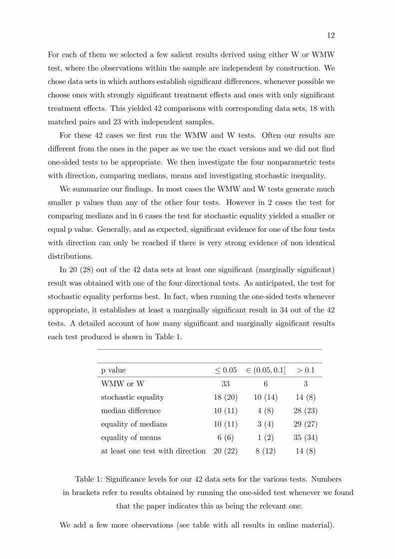
In 20 (28) out of the 42 data sets at least one signi�cant (marginally signi�cant)

result was obtained with one of the four directional tests. As anticipated, the test for

stochastic equality performs best. In fact, when running the one-sided tests whenever

appropriate, it establishes at least a marginally signi�cant result in 34 out of the 42

tests. A detailed account of how many signi�cant and marginally signi�cant results

each test produced is shown in Table 1.

p value � 0:05 2 (0:05; 0:1] > 0:1

WMW or W 33 6 3

stochastic equality 18 (20) 10 (14) 14 (8)

median di¤erence 10 (11) 4 (8) 28 (23)

equality of medians 10 (11) 3 (4) 29 (27)

equality of means 6 (6) 1 (2) 35 (34)

at least one test with direction 20 (22) 8 (12) 14 (8)

Table 1: Signi�cance levels for our 42 data sets for the various tests. Numbers

in brackets refer to results obtained by running the one-sided test whenever we found

that the paper indicates this as being the relevant one.

We add a few more observations (see table with all results in online material).

13

In the extremely small data sets, identi�ed by having between 5 and 7 observations

in each sample, the test for stochastic equality identi�ed a signi�cant �nding in 3

out of the 6 cases. Note that our novel test for testing equality of medians performs

quite well in data sets in which the minimal sample size is at least 15: In 9 out of

22 cases it establishes a signi�cant result. The equality of means test requires larger

samples, the 6 cases with signi�cance were obtained among the 17 cases with at least

25 observations in each sample.

For a subset of the data sets we also derive con�dence sets for the di¤erence in

medians, for the median di¤erence and for the stochastic di¤erence. These nicely

complement our basic tests. In 4 out of the 17 data sets the con�dence set for the

di¤erence in medians contains a single point. This means that one can signi�cantly

identify the di¤erence in medians. One of these nicely highlights the di¤erence be-

tween tests for identity of distributions and for identity of medians. In this data

set with 36 matched pairs there is signi�cant evidence that the two distributions are

di¤erent yet there is also signi�cant evidence that both have the same median.

For the same set of journals and same time period we found 7 papers that use

the Wilcoxon test to compare a single variable to speci�c value or sequence of values.

Symmetry was mentioned only twice but not motivated. We obtained data sets and

the necessary information to replicate the results for 6 of these papers. We chose 9

salient data sets from them and �nd that both the median and the mean analysis

produce signi�cant results in 7 cases, in particular without assuming symmetry.

8 Conclusion

The Wilcoxon-Mann-Whitney and Wilcoxon tests are the most prominent tests for

to identifying that two treatments generate di¤erent outcome distributions. These

two tests are extremely useful for getting a �rst understanding when comparing treat-

ments. In addition, the WMW test stands out due to its unique properties.14 Con-

ventions are important in statistical testing.15 Hence, alternative tests such as the

Kolmogorov-Smirnov test (Kolmogorov, 1933, Smirnov, 1939) should only be used if

they can be justi�ed based on the design of the treatments, irrespective of the speci�c

data gathered. However, neither the WMW nor the W test should be used to make

14The WMW test is uniformly most powerful among all unbiased tests that are invariant to

monotone transformations of the data (Lehmann and Romano, 2005).15Otherwise the user may be tempted to try several di¤erent tests and only report the results of

the one that is most favorable.

14

claims about which method is better. Nor should any other permutation or di¤erent

test for identity of distributions be used for this cause.16

We �nd no justi�cation for using the two sample t test and its robust counterpart

(Welch, 1947) in �nite samples. It is known, yet generally overlooked (see the low

number of citations), that tests based on asymptotic theory can be very inappropriate

in �nite samples (eg see Lehmann and Loh, 1990, Dufour, 2003, Romano, 2004,

Medina, 2010).

In this article, we present eight correct and valid tests and show how useful they

are for understanding real data. We �nd that it is useful to explain evidence in terms

of ordinal di¤erences as one can then apply the test for stochastic inequality. If one

wishes to identify di¤erences in terms of means then the following has to be taken

into account. It is not possible to claim signi�cant evidence of a di¤erence in means

if the underyling random variables have no natural bounds. The samples should not

be too small as in most experimental investigations if one wishes to compare means

(Note that we only obtained sign�cant results in 6 of our data sets, see Table 1).

Statistical testing is a mathematical �eld that naturally requires to make correct

claims. Of course it will not be possible to construct exact tests for each statistical

model of the underlying data generating process. Asymptotic theory remains to be

helpful to guide the design of tests. However, we think that it is only fair to report

on extensive simulations whenever using a test whose �nite sample properties are

not mathematically founded. Oversizedness in these simulations should lead to an

upwards adjustment in the reported p values.

Statistical analysis can have a drastic impact on life, such as when used to design

development policies for the third world or to analyze the e¤ectiveness of new drugs.

As such we think that we owe it to us to do this analysis mathematically correct.

References

[1] Asparouhova, Elena, Peter Bossaerts, Jon Eguia, and William Zame, �Asset

Pricing and Asymmetric Reasoning,�Journal of Political Economy, 123 (2015),

66-122.

[2] Bahadur, R. R., and Leonard J. Savage, �The Nonexistence of Certain Statistical

Procedures in Nonparametric Problems,�The Annals of Mathematical Statistics,

16Note that the test used in Cohen and Dupas (2010) is a permutation test that is misused to

identify di¤erences in means.

15

27 (1956), 1115�1122.

[3] Becchetti, Leonardo, Maurizio Fiaschetti, and Giancarlo Marini, �Card Games

and Economic Behavior,�Games and Economic Behavior, 88 (2014), 112�129.

[4] Bhattacharya, Sourav John Du¤y, and Sun-Tak Kim, �Compulsory Versus Vol-

untary Voting: An Experimental Study,�Games and Economic Behavior, 84

(2014), 111�131.

[5] Brocas, Isabelle, Juan D. Carillo, Stephie W. Wang, and Colin F. Camerer,

�Imperfect Choice or Imperfect Attention? Understanding Strategic Thinking

in Private Information Games,��Review of Economic Studies (2014), 81, 944�

970.

[6] Brunner, Edgar and Ullrich Munzel (2000), �The Nonparametric Behrens-Fisher

Problem: Asymptotic Theory and a Small-Sample Approximation,�Biometrical

Journal, 42, 17-25.

[7] Cabral, Luis, Erkut Y. Ozbay, and Andrew Schotter, �Intrinsic and Instrumen-

tal Reciprocity: An Experimental Study,�Games and Economic Behavior, 87

(2014), 100�121.

[8] Cason, Timothy N., Daniel Friedman, and Ed Hopkins, �Cycles and Instability

in a Rock�Paper�Scissors Population Game: A Continuous Time Experiment,�

Review of Economic Studies (2014), 81, 112�136.

[9] Cason, Timothy N., and Charles R. Plott, �Misconceptions and Game Form

Recognition: Challenges to Theories of Revealed Preference and Framing,�Jour-

nal of Political Economy, 122 (2014), 1235-1270.

[10] Charness, Gary, Ramón Cobo-Reyes, and Natalia Jiménez, �Identities, Selection,

and Contributions in a Public-Goods Game,�Games and Economic Behavior,

87 (2014), 322�338.

[11] Chen, Yan, Sherry Xin Li, Tracy Xiao Liu, and Margaret Shih, �Which Hat to

Wear? Impact of Natural Identities on Coordination and Cooperation,�Games

and Economic Behavior, 84 (2014), 58�86.

[12] Cheung, Stephen L., �Comment on �Risk Preferences Are Not Time Prefer-

ences�: On the Elicitation of Time Preference under Conditions of Risk,�Amer-

ican Economic Review, 105 (2015), 2242�2260.

16

[13] Chung, EunYi, Romano, Joseph P., �Exact and Asymptotically Robust Permu-

tation Tests,�The Annals of Statistics, 41 (2015), 484�507.

[14] Cohen, Jessica, and Pascaline Dupas, �Free Distribution or Cost-Sharing? Evi-

dence from a Randomized Malaria Prevention Experiment,�The Quarterly Jour-

nal of Economics, 75 (2010), 1-45.

[15] Cohn, Alain, Jan Engelmann, Ernst Fehr, and Michel André Maréchal, �Evi-

dence for Countercyclical Risk Aversion: An Experiment with Financial Profes-

sionals,�American Economic Review, 105 (2015), 860�885.

[16] Dittmann, Ingolf, Dorothea Kübler, Ernst Maug, and Lydia Mechtenberg, �Why

Votes have Value: Instrumental Voting with Overcon�dence and Overestimation

of Others�Errors,�Games and Economic Behavior, 84 (2014), 17�38.

[17] Du¤y, John, and Daniela Puzzello, �Gift Exchange versus Monetary Exchange:

Theory and Evidence,�American Economic Review, 104 (2014), 1735�1776.

[18] Dufour, Jean-Marie, �Identi�cation, Weak Instruments, and Statistical Infer-

ence in Econometrics,�The Canadian Journal of Economics / Revue canadienne

d�Economique, 36 (2003), 767-808.

[19] Dufour, Jean-Marie, and Marc Hallin, �Improved Eaton Bounds for Linear Com-

binations of Bounded Random Variables, with Statistical Applications,�Journal

of the American Statistical Association, 88 (1993), 1026�1033.

[20] Eckel, Catherine C., and Sascha C. Füllbrunn, �Thar SHE Blows? Gender,

Competition, and Bubbles in Experimental Asset Markets,�American Economic

Review, 105 (2015), 906�920.

[21] FDA, Regulatory Information, Statistical Guidance for Clinical Trials of Non

Diagnostic Medical Devices, The Division of Biostatistics, U.S. Food and Drug

Administration, 1996.

[22] FDA, Redbook 2000, Guidance for Industry and Other Stakeholders Toxicolog-

ical Principles for the Safety Assessment of Food Ingredients, U.S. Department

of Health and Human Services, Food and Drug Administration, Center for Food

Safety and Applied Nutrition, 2007.

[23] Feltovich, Nick, �Critical values for the robust rank-order test�, Communications

in Statistics - Simulation and Computation, 34 (2005), 525-547.

17

[24] Filiz-Ozbay, Emel, Kristian Lopez-Vargas, and Erkut Y.Ozbay, �Multi-Object

Auctions with Resale: Theory and Experiment,�Games and Economic Behavior,

89 (2015) 1�16.

[25] Fisher, R. A. (1935), �The Logic of Inductive Inference,�J. Roy. Stat. Soc. 98,

39�54.

[26] Fligner, Michael A., and George E. Policello II, �Robust Rank Procedures for

the Behrens-Fisher Problem,�Journal of the American Statistical Association,

76 (1981), 162-168.

[27] Forsythe, Robert, Joel L. Horowitz, N. E. Savin, and Martin Sefton, �Fairness

in Simple Bargaining Experiments,�Games and Economic Behavior, 6 (1994),

347�369.

[28] Friedman, Daniel, Ste¤en Huck, Ryan Oprea, and Simon Weidenholzer, �From

Imitation to Collusion: Long-run Learning in a Low-Information Environment,�

Journal of EconomicTheory, 155 (2015), 185�205.

[29] Hugh-Jones, David, Morimitsu Kurino, and Christoph Vanberg, �An Experi-

mental Study on the Incentives of the Probabilistic Serial Mechanism,�Games

and Economic Behavior, 87 (2014), 367�380.

[30] Isoni, Andrea, Anders Poulsen, Robert Sugden, and Kei Tsutsui, �E¢ ciency,

Equality, and Labeling: An Experimental Investigation of Focal Points in Ex-

plicit Bargaining,�American Economic Review, 104 (2014), 3256�3287.

[31] Kamijoa, Y., T. Nihonsugi, A. Takeuchi, and Y. Funaki, �Sustaining Coopera-

tion in Social Dilemmas: Comparison of Centralized Punishment Institutions,�

Games and Economic Behavior, 84 (2014), 180�195.

[32] Kiryl Khalmetskia, Axel Ockenfels, and Peter Werner, �Surprising Gifts:Theory

and Laboratory Evidence,�Journal of Economic Theory, 159 (2015), 163�208.

[33] Kolmogorov A., �Sulla Determinazione Empirica di una Legge di Distribuzione,�

Giornale dell�Istituto Italiano degli Attuari, 4 (1933), 83�91.

[34] Kosfeld, Michael and Devesh Rustagi, �Leader Punishment and Cooperation in

Groups: Experimental Field Evidence from Commons Management in Ethiopia,�

American Economic Review, 105 (2015), 747�783.

18

[35] Lai, Ernest K., Wooyoung Lim, and Joseph Tao-yi Wang, �An Experimental

Analysis of Multidimensional Cheap Talk,�Games and Economic Behavior, 91

(2015), 114�144.

[36] Lehmann, E. L., and Wei-Yin Loh (1990), �Pointwise verses Uniform Robustness

in some Large-Sample Tests and Con�dence Intervals,�Scandinavian Journal of

Statistics, 17, 177�187.

[37] Lehmann, Erich L., and Joseph P. Romano, Testing Statistical Hypotheses, New

York: Springer, 2005.

[38] Mann, H. B., and D. R. Whitney, �On a Test Whether One of Two Random

Variables is Stochastically Larger Than the Other,�Annals of Mathematical Sta-

tistics, 18 (1947), 50�60.

[39] Markussen, Thomas, Louis Putterman, and Jean-Robert Tyran, �Self-

Organization for Collective Action: An Experimental Study of Voting on Sanc-

tion Regimes,�Review of Economic Studies, 81 (2014) , 301�324.

[40] Masella, Paolo, Stephan Meier, and Philipp Zahn, �Incentives and Group Iden-

tity,�Games and Economic Behavior, 86 (2014), 12�25.

[41] McNemar, Q., �Note on the Sampling Error of the Di¤erence Between Correlated

Proportions or Percentages,�Psychometrika, 12 (1947), 153�157.

[42] Medina, Jared, Daniel Y. Kimberg, Anjan Chatterjee, and H. Branch Coslett,

�Inappropriate Usage of the Brunner-Munzel Test in Recent Voxelbased Lesion-

Symptom Mapping Studies,�Neuropsychologia, 48 (2010), 341�343.

[43] Miao, Bin and Songfa Zhong, �Comment on �Risk Preferences Are Not Time

Preferences�: Separating Risk and Time Preference,�American Economic Re-

view, 105 (2015), 2272�2286.

[44] Mood, A.M., Introduction to the Theory of Statistics, New York: McGraw-Hill,

1950.

[45] Noussair, Charles N., Stefan T. Trautmann, and Gijs van de Kuilen, �Higher

Order Risk Attitudes, Demographics, and Financial Decisions,�Review of Eco-

nomic Studies, 81 (2014), 325�355.

[46] Ockenfels, Axel, and Reinhard Selten, �Impulse Balance in the News Vendor

Game,�Games and Economic Behavior, 86 (2014), 237�247.

19

[47] Oprea, Ryan, �Survival Versus Pro�t Maximization in a Dynamic Stochastic

Experiment,�Econometrica, 82 (2014), 2225�2255.

[48] Romano, Joseph P., �On Non-Parametric Testing, the Uniform Behaviour of the

t-Test, and Related Problems,� Scandinavian Journal of Statistics, 31 (2004),

567-584.

[49] Petersen, Luba, and Abel Winn, �Does Money Illusion Matter?: Comment,�

American Economic Review, 104 (2014), 1047�1062.

[50] Pratt, J. W., �Remarks on Zeros and Ties in the Wilcoxon Signed Rank Proce-

dures,�Journal of the American Statistical Association 54 (1959), 655-667.

[51] Regner, Tobias, �Social Preferences? Google Answers!,�Games and Economic

Behavior, 85 (2014), 188�209.

[52] Romano, Joseph P., and Michael Wolf, �Finite Sample Non-Parametric Inference

and Large Sample E¢ ciency,�Annals of Statistics, 28 (2000), 756�778.

[53] Schlag, Karl H., �A New Method for Constructing Exact Tests without Making

any Assumptions,�Department of Economics and Business Working Paper, 1109

(2008a), Universitat Pompeu Fabra.

[54] Schlag, Karl H., Exact Hypothesis Testing without Assumptions - New

and Old Results not only for Experimental Game Theory, mimeo,

http://homepage.univie.ac.at/karl.schlag/research/statistics/exacthypothesistesting.pdf,

2011.

[55] Shapiro, Dmitry, Xianwen Shi, and Artie Zillante, �Level-k Reasoning in a Gen-

eralized Beauty Contest,�Games and Economic Behavior, 86 (2014), 308�329.

[56] Siegel, Sidney and N. John Castellan Jr., Nonparametric Statistics for The Be-

havioral Sciences, 2nd ed. (McGraw-Hill), 1988.

[57] Smirnov, N. V., �Estimate of Deviation Between Empirical Distribution Func-

tions in Two Independent Samples,�Bulletin Moscow University 2 (1939), 3�16.

[58] Spearman, C., �The Proof and Measurement of Association Between Two

Things,�The American Journal of Psychology, 15 (1904), 72�101.

[59] Student, �The Probable Error of a Mean,�Biometrika 6 (1908), 1�25.

20

[60] Suissa, Samy, and Jonathan J. Shuster, �Exact Unconditional Sample Sizes for

the 2 � 2 Binomial Trial,� Journal of the Royal Statistitical Society, Series A,148 (1985), 317�327.

[61] Suissa, Samy, and Jonathan J. Shuster, �The 2 x 2 Matched-Pairs Trial: Exact

Unconditional Design and Analysis,�Biometrics, 47 (1991), 361�372.

[62] Tocher, K. D., �Extension of the Neyman-Pearson Theory of Tests to Discontin-

uous Variates,�Biometrika, 37 (1950), 130�144.

[63] Wantchekon, Leonard, Marko Klasnja, and Natalija Novta, �Education and Hu-

man Capital Externalities: Evidence from Colonial Benin,�The Quarterly Jour-

nal of Economics, 130 (2015), 703�757.

[64] Welch, B. L., �The Generalization of �Student�s�Problem when Several Di¤erent

Population Variances are Involved,�Biometrika, 34 (1947), 28-35.

[65] Westenberg, J., �Signi�cance Test for Median and Interquartile Range in Samples

from Continuous Populations of Any Form,� form,�Proceedings of the Konin-

klijke Nederlandse Akademie van Wetenschapp, 51 (1948), 252-261.

[66] Wilcoxon, F., �Individual Comparisons by Ranking Methods,�Biometrics Bul-

letin, 1 (1945), 80�83.

[67] Yates, F., �Contingency Tables Involving Small Numbers and the �2 Test,�Sup-

plement to the Journal of the Royal Statistical Society, 1 (1934), 217�235.

21

A Figures on Oversizedness

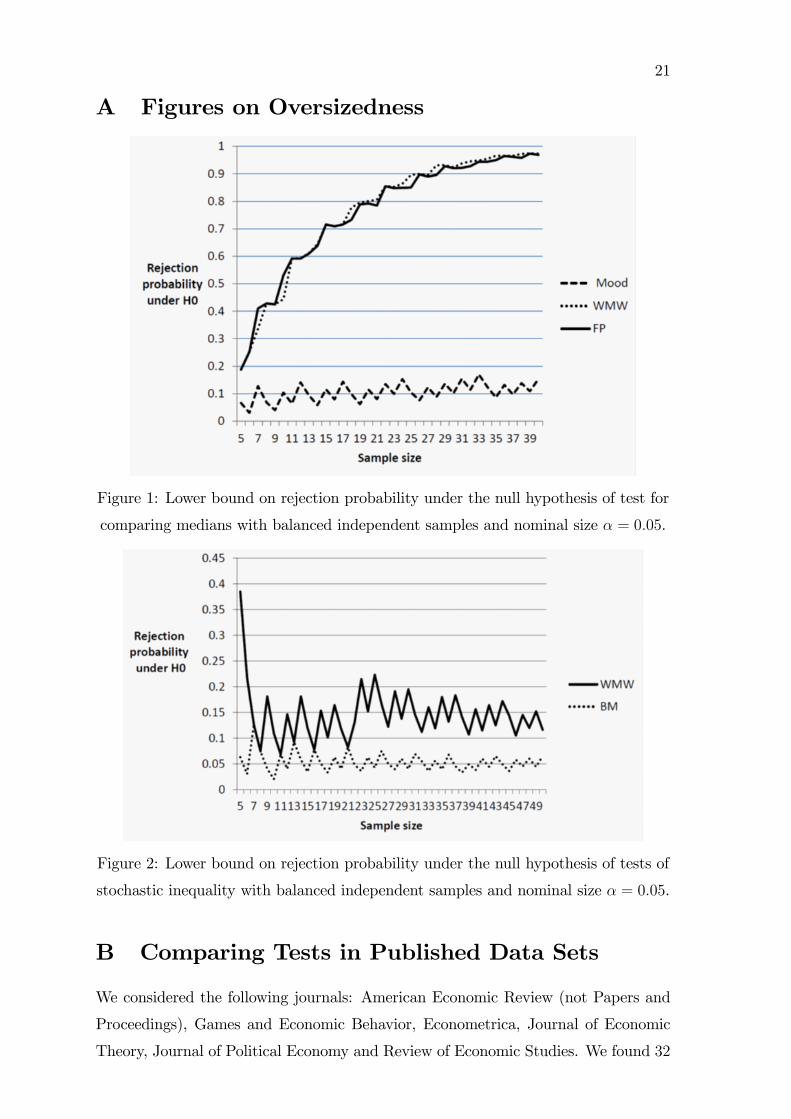
Figure 1: Lower bound on rejection probability under the null hypothesis of test for

comparing medians with balanced independent samples and nominal size � = 0:05.

Figure 2: Lower bound on rejection probability under the null hypothesis of tests of

stochastic inequality with balanced independent samples and nominal size � = 0:05.

B Comparing Tests in Published Data Sets

We considered the following journals: American Economic Review (not Papers and

Proceedings), Games and Economic Behavior, Econometrica, Journal of Economic

Theory, Journal of Political Economy and Review of Economic Studies. We found 32

22

papers that either use the Wilcoxon-Mann-Whitney or the Wilcoxon test. We were

able to obtain the data and the necessary information to replicate the �ndings for 22

of these papers, either from online sources or directly from the authors. For each of

these papers we selected a few salient hypotheses involving comparing two variables

in which the WMW and W tests can be formally applied, so where observations are

independent. Whenever possible we selected data both where p values of these two

tests were below 0:01 and where they were between 0:01 and 0:05:

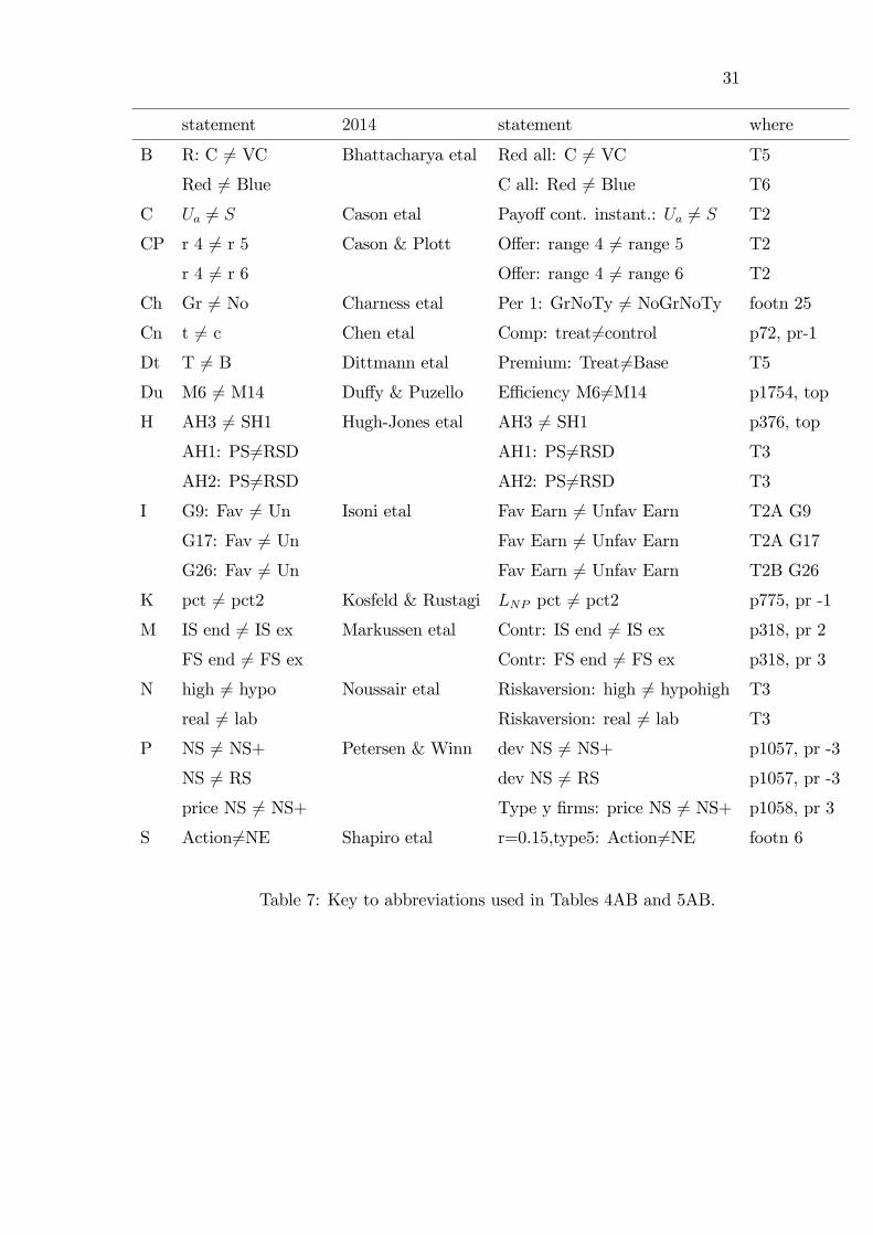
We summarize our �ndings in a series of tables followed by a �key for abbrevia-

tions�table in which more information about the data source is given. In particular,

we identify for each of the hypotheses the authors of the article, enough information

to identify which two variables are being considered and where in the published paper

the relevant statement for WMW or W can be found. In the column �x�we mention

whether we found that the authors are interested in providing evidence of inequality,

highlighted by �6=�or instead where a directional hypothesis can be identi�ed fromthe formulation of the problem as being of central interest.

For each hypothesis we reran the Wilcoxon-Mann-Whitney and Wilcoxon tests,

using the exact versions. Then we ran the four tests for identifying direction as de-

scribed in the main article. For each test, in the column �r�, we highlight the direction

of the evidence whenever it is signi�cant at 5%; put it in brackets if only signi�cant

at 10%: While the cases where one-sided tests are of importance is highlighted in

column �x�, all p values in these two tables refer to the two-sided tests.

The equality of medians test is introduced for the �rst time in this article. It tests

H0 : med (X1) = med (X2) : In our tables we include an ad-hoc measure m̂ of the

evidence that the two medians are di¤erent. It is given by the di¤erence between the

number of observations in each sample that are above the common sample median,

normalized by the number of observations in each sample. Formally, m̂ is de�ned by

m̂ =jfk : x1k � med (fxijg)gj

n1� jfk : x2k � med (fxijg)gj

n2;

where xij is the jth observation in the sample of Xi:

The median di¤erence test is concerned withH0 : med (X1 �X2) = 0: The test for

independent samples follows the lines of the test for stochastic inequality introduced

in (Schlag, 2008). The test for matched pairs is easily designed using the binomial

test. The estimated median di¤erence is denoted by m (x1 � x2) : For matched pairsm (x1 � x2) is given by the median of the sample di¤erences. For independent sam-ples the estimate is given by the expected value that is obtained by �rst forming

min fn1; n2g random pairs, one observation from each sample, and then proceeding

23

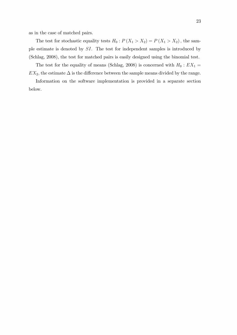
as in the case of matched pairs.

The test for stochastic equality tests H0 : P (X1 > X2) = P (X1 > X2) ; the sam-

ple estimate is denoted by SI. The test for independent samples is introduced by

(Schlag, 2008), the test for matched pairs is easily designed using the binomial test.

The test for the equality of means (Schlag, 2008) is concerned with H0 : EX1 =

EX2; the estimate� is the di¤erence between the sample means divided by the range.

Information on the software implementation is provided in a separate section

below.

24

2015

WMWorW

stochasticequality

mediandi¤erence

statement

xn1;n

2pvalue

rpvalue

rSI

pvalue

rm(x1�x2)

AG26=G3

6=12m

0:06

(6=)

0:04(!!!)

>0:67

0:04

>2:13

G26=G4

6=12m

0:005

6=0:04

>0:67

0:04

>3:86

CgCert6=Ind

6=63m

10�9

6=10�4

>0:56

0:31

20

Ind6=Corr

6=63m

0:015

6=0:08

(>)

0:21

10

Cert6=Corr

6=63m

0:04

6=0:08

(<)�0:17

10

r5:Ind6=Corr6=

63m

0:001

6=0:001(!!!)

>0:38

0:21

9

EBias:m6=f

6=6;6

0:004

6=0:04

>0:94

0:04

>95:5

Turn:m6=f

6=6;6

0:03

6=0:09

(<)�0:75

0:09

(<)

�2:9

FDs:p16=p25

>18m

0:02

6=0:1w

(<)�0:44

0:1w

(<)

�1:87

Tl:b16=b3

6=6m

0:03

6=0:04

>1

0:04

>0:95

LF26=F1

>4;4

0:03

6=0:13

z1

0:13

z0:09

MCer6=Pos

6=111m

10�5

6=10�4

>0:2

10

Pos6=Neg

6=111m

10�4

6=10�4(!!!)

>0:32

120

Cer6=Pos,16

6=111m

0:04

6=0:06

(>)

0:1

10

OI-HS6=I-LS

>28;26

10�8

6=10�5

>0:82

10�5

>0:35

WK:t6=nw/o

>89;151

10�6

6=10�4

>0:39

0:004

>2

D:t6=nw

>89;154

0:005

6=0:05

>0:22

0:64

1

Table2:Summaryof�ndingsfor2015papers:pvaluesforWMWorW,stochasticinequalityandmediandi¤erence.

25

2015

WMWorW

equalityofmedians

equalityofmeans

statement

xn1;n

2pvalue

rpvalue

rm̂

pvalue

rrange

�

AG26=G3

6=12m

0:06

(6=)

0:56

0:33

1[0;18]y

0:096

G26=G4

6=12m

0:005

6=0:56

0:33

1[0;18]y

0:16

CgCert6=Ind

6=63m

10�9

6=10�6

>0:43

0:001

>[0;100]

0:23

Ind6=Corr

6=63m

0:015

6=0:25

0:11

0:59

[0;100]

0:09

Cert6=Corr

6=63m

0:04

6=0:05

<0e*

0:4

[0;100]

�0:09

r5:Ind6=Corr6=

63m

0:001

6=0:57

0:25

0:27

[0;100]

0:13

EBias:m6=f

6=6;6

0:004

6=0:08

(>)

0:67

0:21

[�80;140]y

0:45

Turn:m6=f

6=6;6

0:03

6=0:3

�0:67

0:95

[5;25]y

�0:23

FDs:p16=p25

>18m

0:02

6=0:19

z�0:33

0:94

[0;8]y

�0:071

Tl:b16=b3

6=6m

0:03

6=toosmall

1[0;5]y

0:15

LF26=F1

>4;4

0:03

6=0:25

11

[0;1]

0:096

MCer6=Pos

6=111m

10�5

6=0:001

>0:18

0:003

>[0;100]

0:13

Pos6=Neg

6=111m

10�4

6=10�6(!!)

<�0:13e

0:02

>[0;100]

0:16

Cer6=Pos,16

6=111m

0:04

6=0:006(!!)

>0:099

0:55

[0;100]

0:056

OI-HS6=I-LS

>28;26

10�8

6=0:001

>0:63

0:002

>[0;1]

0:34

WK:t6=nw/o

>89;151

10�6

6=0:03

>0:27

0:02

>[0;20]

0:12

D:t6=nw

>89;154

0:005

6=0:37

0:13

z0:5

[0;41]

0:045

Table3:Summaryof�ndingsfor2015papers:pvaluesforWMWorW,equalityofmediansandmeans.

26

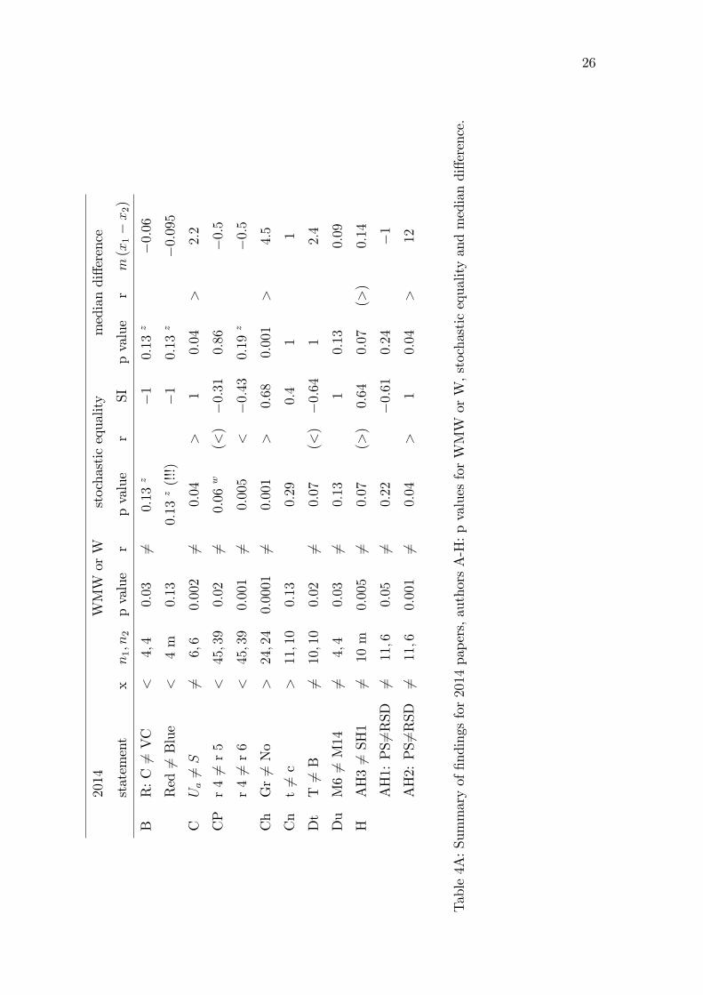
2014

WMWorW

stochasticequality

mediandi¤erence

statement

xn1;n

2pvalue

rpvalue

rSI

pvalue

rm(x1�x2)

BR:C6=VC

<4;4

0:03

6=0:13

z�1

0:13

z�0:06

Red6=Blue

<4m

0:13

0:13

z(!!!)

�1

0:13

z�0:095

CUa6=S

6=6;6

0:002

6=0:04

>1

0:04

>2:2

CP

r46=r5

<45;39

0:02

6=0:06

w(<)�0:31

0:86

�0:5

r46=r6

<45;39

0:001

6=0:005

<�0:43

0:19

z�0:5

Ch

Gr6=No

>24;24

0:0001

6=0:001

>0:68

0:001

>4:5

Cn

t6=c

>11;10

0:13

0:29

0:4

11

Dt

T6=B

6=10;10

0:02

6=0:07

(<)�0:64

12:4

Du

M66=M14

6=4;4

0:03

6=0:13

10:13

0:09

HAH36=SH1

6=10m

0:005

6=0:07

(>)

0:64

0:07

(>)

0:14

AH1:PS6=RSD

6=11;6

0:05

6=0:22

�0:61

0:24

�1

AH2:PS6=RSD

6=11;6

0:001

6=0:04

>1

0:04

>12

Table4A:Summaryof�ndingsfor2014papers,authorsA-H:pvaluesforWMWorW,stochasticequalityandmediandi¤erence.

27

2014

WMWorW

stochasticequality

mediandi¤erence

statement

xn1;n

2pvalue

rpvalue

rSI

pvalue

rm(x1�x2)

IG9:Fav6=Un

>36m

0:04

6=0:11

z0:17

10

G17:Fav6=Un

>36m

0:003

6=0:002(!!!)

>0:44

0:62

1

G26:Fav6=Un

>42m

0:06

(6=)

0:12

z0:21

10

Kpct6=pct2

>16m

0:003

6=0:02

>0:63

0:03

>25:3

MISend6=ISex

>6;4

0:02

6=0:15

z0:92

0:15

z4:5

FSend6=FSex

>9;7

0:07

(6=)

0:27

0:56

0:27

2:35

Nhigh6=hypo

6=1065;994

10�10a

6=10�10(!!!)

<�0:21

10

real6=lab

6=1395;109

0:09

(6=)

0:24

�0:095

10

PNS6=NS+

6=19;19

0:06

(6=)

0:19

0:37

0:23

2:25

NS6=RS

6=19;15

0:02

6=0:09

(>)

0:48

0:29

3

priceNS6=NS+

6=7;5

0:03

6=0:16

�0:71

0:72

�1

SAction6=NE

6=5m

0:07

(6=)

0:07

(>)

10:07

(>)

15:78

Table4B:Summaryof�ndingsfor2014papersauthorsI-Z:pvaluesforWMWorW,stochasticequalityandmediandi¤erence.

28

2014

WMWorW

equalityofmedians

equalityofmeans

statement

xn1;n

2pvalue

rpvalue

rm̂

pvalue

rrange

�

BR:C6=VC

<4;4

0:03

6=0:25

�1

0:43

[0:85;1]y

�0:4

Red6=Blue

<4m

0:13

toosmall

0:81

[0:85;1]y

�0:58

CUa6=S

6=6;6

0:002

6=0:07

(>)

10:06

(>)

[47;51]y

0:56

CP

r46=r5

<45;39

0:02

6=0:43

�0:18

0:99

[0;5]

�0:074

r46=r6

<45;39

0:001

6=0:06

w(<)�0:21

0:85

[0;6]

0:086

Ch

Gr6=No

>24;24

0:0001

6=0:02

>0:5

0:12

z[0;25]

0:19

Cn

t6=c

>11;10

0:13

10:31

0:76

[1;7]

0:15

Dt

T6=B

6=10;10

0:02

6=0:44

�0:4

0:25

[�1;8]

�0:28

Du

M66=M14

6=4;4

0:03

6=0:25

11

[0;1]

0:095

HAH36=SH1

6=10m

0:005

6=0:31

0:46

1[0;1]

0:14

AH1:PS6=RSD

6=11;6

0:05

6=0:56

�0:47

0:94

[91;97]

�0:19

AH2:PS6=RSD

6=11;6

0:001

6=0:05

>0:818

0:11

[70;97]

0:45

Table5A:Summaryof�ndingsfor2014papers,authorsA-H:pvaluesforWMWorW,equalityofmediansandmeans.

29

2014

WMWorW

equalityofmedians

equalityofmeans

statement

xn1;n

2pvalue

rpvalue

rm̂

pvalue

rrange

�

IG9:Fav6=Un

>36m

0:04

6=1

0:17

1[0;10]y

0:025

G17:Fav6=Un

>36m

0:003

6=0:58

0:47

1[0;10]y

0:053

G26:Fav6=Un

>42m

0:06

(6=)

10:14

1[0;10]y

0:064

Kpct6=pct2

>16m

0:003

6=0:19

z0:5

1[0;200]y

0:11

MISend6=ISex

>6;4

0:02

6=0:21

0:83

1[0;20]

0:2

FSend6=FSex

>9;7

0:07

(6=)

0:43

0:38

1[0;20]

0:11

Nhigh6=hypo

6=1065;994

10�10a

6=0:002

<�0:18

10�8b

<[0;5]

�0:115

real6=lab

6=1395;109

0:09

(6=)

1�0:11

0:17

b[0;5]

�0:079

PNS6=NS+

6=19;19

0:06

(6=)

0:48

0:26

0:86

[�3;25]y

0:098

NS6=RS

6=19;15

0:02

6=0:14

0:35

0:84

[�2;25]y

0:11

priceNS6=NS+

6=7;5

0:03

6=0:78

�0:71

0:98

[�4;1]y

�0:2

SAction6=NE

6=5m

0:07

(6=)

toosmall

0:88

[44;80]y

0:46

Table5B:Summaryof�ndingsfor2014papersauthorsI-Z:pvaluesforWMWorW,equalityofmediansandmeans.

30

statement 2015 statement where

A G2 6= G3 Asparouhova etal Mispricing: G2 6= G3 p90, pr-1

G2 6= G4 Mispricing: G2 6= G4 p90, pr-1

Cg Cert 6= Ind Cheung Cert 6= Ind T2, row 1

Ind 6= Corr Ind 6= Corr T2, row 3

Cert 6= Corr Cert 6= Corr T2, row 4

r5: Ind 6= Corr Ind 6= Corr T2, row 5

E Bias: m 6= f Eckel etal Avgbias: all m 6= all f p911, pr-1

Turn: m 6= f Turnover: all m 6= all f p911, pr-1

F Ds: p1 6= p25 Friedman etal Duo short: per 1 6= per 25 p192, pr1

Tl: b1 6= b3 Tri long: block 1 6= block 3 p193 pr-3

L F26=F1 Lai etal F(Game 2)6=F(Game 1) T3

M Cer6=Pos Miao & Zhong Cer6=Pos, g1 1-5 TA1

Pos6=Neg Pos6=Neg, g1 1-5 TA1

Cer6=Pos, 16 Cer6=Pos, g1 5-16 TA1

O I-HS 6= I-LS Oprea Invest: I-HS 6= I-LS p2248, pr1

W K: t 6= n w/o Wantchekon etal Kids: treat 6= no treat w/o sch TXII

D: t 6= n w Desc.: treat 6= no treat w sch TXII

Table 6: Key to abbreviations used in Tables 2 and 3.

31

statement 2014 statement where

B R: C 6= VC Bhattacharya etal Red all: C 6= VC T5

Red 6= Blue C all: Red 6= Blue T6

C Ua 6= S Cason etal Payo¤ cont. instant.: Ua 6= S T2

CP r 4 6= r 5 Cason & Plott O¤er: range 4 6= range 5 T2

r 4 6= r 6 O¤er: range 4 6= range 6 T2

Ch Gr 6= No Charness etal Per 1: GrNoTy 6= NoGrNoTy footn 25

Cn t 6= c Chen etal Comp: treat6=control p72, pr-1

Dt T 6= B Dittmann etal Premium: Treat6=Base T5

Du M6 6= M14 Du¤y & Puzello E¢ ciency M66=M14 p1754, top

H AH3 6= SH1 Hugh-Jones etal AH3 6= SH1 p376, top

AH1: PS6=RSD AH1: PS6=RSD T3

AH2: PS6=RSD AH2: PS6=RSD T3

I G9: Fav 6= Un Isoni etal Fav Earn 6= Unfav Earn T2A G9

G17: Fav 6= Un Fav Earn 6= Unfav Earn T2A G17

G26: Fav 6= Un Fav Earn 6= Unfav Earn T2B G26

K pct 6= pct2 Kosfeld & Rustagi LNP pct 6= pct2 p775, pr -1

M IS end 6= IS ex Markussen etal Contr: IS end 6= IS ex p318, pr 2

FS end 6= FS ex Contr: FS end 6= FS ex p318, pr 3

N high 6= hypo Noussair etal Riskaversion: high 6= hypohigh T3

real 6= lab Riskaversion: real 6= lab T3

P NS 6= NS+ Petersen & Winn dev NS 6= NS+ p1057, pr -3

NS 6= RS dev NS 6= RS p1057, pr -3

price NS 6= NS+ Type y �rms: price NS 6= NS+ p1058, pr 3

S Action6=NE Shapiro etal r=0.15,type5: Action6=NE footn 6

Table 7: Key to abbreviations used in Tables 4AB and 5AB.

32

Explaining symbols used in Tables: 2,3,$AB,5AB

� all tests are two-sided

� all p values rounded up, reported on the grid 10�10; ::; 10�4; 0:001; ::; 0:009; andabove to two decimals behind the comma

� WMW and W use exact distribution, W deals with ties as in Pratt (1959) to

be comparable to STATA although STATA uses asymptotic p values.

� �T�stands for table

� �pr�stands for paragraph

� �x�indicates desired alternative hypothesis in paper

� �m�refers to matched pairs

� �r�refers to signi�cant evidence at level 0:05 of the two-sided test, in bracketsif marginally signi�cant at level 0:1

� �̂m�adhoc measure of di¤erence in medians, de�ned as di¤erence of proportionof observations above the common median

� �*�: instance where m̂ = 0 but medians are di¤erent, given by 0 and 20:

� �e�: one of the sample medians is at the extreme points of data range

� �range�indicates range of outcomes used for running test for comparing means

� �y�indicates that range chosen more or less arbitrarily based on data, so infer-ence is conditional on outcomes belonging to that interval

� �SI�: estimate of the stochastic inequality, given by the di¤erence in the propor-tions of matches in which observation in �rst sample greater and smaller

� ���: di¤erence in means normalized by the range

� �(!!)�highlights that p value of median test less or equal to that of W or WMW

test

� �(!!!)�highlights that p value of median test less or equal to that of W or WMW

test

� �b�: in means test with very large data sets we exogenously choose � = 0:3

33

� �too small�: indicates that sample size too small for sensible results, for thesesample sizes no data can lead to p value below 0:2 with our median test

� �z�: the authors are interested in a one-sided test, for this the result is marginallysigni�cant (p value at most 0:1)

� �w�: the authors are interested in a one-sided test, for this the result is signi�cant(p value at most 0:05)

C Con�dence Intervals

For a subset of the above data we compute con�dence intervals for the three tests

that involve ordinal comparisons.

34

35

Con�denceIntervals

stochasticdi¤erence

mediandi¤erence

P(X

1>X2)�P(X

1<X2)

med(X

1�X2)

statement

where

n1;n

295%CI

SI95%CI

m(x1�x2)

Friedmanetal(2015)

Duoshort:per16=per25

p192,pr1

18m

[�0:81;0:06]

�0:44

[�2:6;0:08]

�1:87

Isoni(2014)

FavEarn6=UnfavEarn

T2A

G9

36m

[�0:11;0:94]

0:167

[0;0]

0

FavEarn6=UnfavEarn

T2B

G26

42m

[�0:07;0:66]

0:21

[0;1:5]

0

Cheung(2015)

Cert6=Ind

T2,row1

63m

[0:8;1]

0:56

[0;45]

20

Ind6=Corr

T2,row3

63m

[�0:02;0:54]

0:21

[0;10]

0

Miao&Zhong(2015)

Cer6=Pos,g11-5

TA1

111m

[0:5;0:98]

0:2

[0;0]

0

Eckeletal(2015)

Avgbias:allm6=allf

p911,pr-1

6;6

[0:05;0:99]

0:94

[13;178]

95

Chenetal(2014)

Comp:treat6=control

p72,pr-1

11;10

[�0:35;0:93]

0:4

[0;3]

1

Petersen&Winn(2014)

devNS6=NS+

p1057,pr-3

19;19

[�0:12;0:74]

0:37

[�0:7;5:7]

2:2

devNS6=RS

p1057,pr-3

19;15

[�0:06;0:88]

0:48

[0;6]

3

Charnessetal(2014)

Per1:GrNoTy6=NoGrNoTy

footn25

24;24

[0:28;0:9]

0:68

[1:2;8:9]

4:5

Oprea(2015)

Invest:I-HS6=I-LS

p2248,pr1

28;26

[0:5;0:95]

0:82

[0:14;0:54]

0:35

Cason&Plott(2014)

O¤er:range46=range5

T2

45;39

[�0:7;0:01]

�0:31

[�0:86;0]

�0:5

Wantchekonetal(2015)

Kids:treat6=notreatw/osch

TXII

89;151

[0:18;0:62]

0:39

[1;3]

2

Desc.:treat6=notreatwsch

TXII

89;154

[0:01;0:47]

0:22

[0;3]

1

Noussairetal(2014)

Riskaversion:high6=hypohigh

T3

1065;994

[�0:4;�0:15]

�0:21

[�1;0]

0

Riskaversion:real6=lab

T3

1395;109

[�0:37;0:12]

�0:095

[�1;0]

0

Table8A:Summaryof�ndings:con�denceintervalsforstochasticandmediandi¤erence

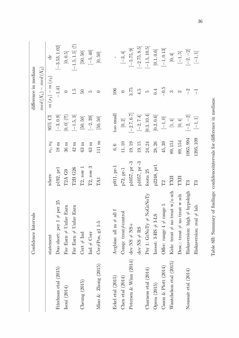
36

Con�denceIntervals

di¤erenceinmedians

med(X

1)�med(X

2)

statement

where

n1;n

295%CI

m(x1)�m(x2)

dr

Friedmanetal(2015)

Duoshort:per16=per25

p192,pr1

18m

[�3;0:9]

�1:41

[�3:53;1:02]

Isoni(2014)

FavEarn6=UnfavEarn

T2A

G9

36m

[0;0](!!)

0[0;0:5]

FavEarn6=UnfavEarn

T2B

G26

42m

[�1:5;3]

1:5

[�1:5;1:5](!)

Cheung(2015)

Cert6=Ind

T2,row1

63m

[50;50]

50[50;50]

Ind6=Corr

T2,row3

63m

[�2;39]

5[�5;40]

Miao&Zhong(2015)

Cer6=Pos,g11-5

TA1

111m

[50;50]

0[0;50]

Eckeletal(2015)

Avgbias:allm6=allf

p911,pr-1

6;6

toosmall

106

-

Chenetal(2014)

Comp:treat6=control

p72,pr-1

11;10

[0;2]

0[�3;4]

Petersen&Winn(2014)

devNS6=NS+

p1057,pr-3

19;19

[�2:7;6:7]

3:75

[�5:75;9]

devNS6=RS

p1057,pr-3

19;15

[�2;7:4]

4:5

[�2:75;8:5]

Charnessetal(2014)

Per1:GrNoTy6=NoGrNoTy

footn25

24;24

[0:3;10:4]

5[�1:5;10:5]

Oprea(2015)

Invest:I-HS6=I-LS

p2248,pr1

28;26

[0:2;0:6]

0:4

[0:1;0:6]

Cason&Plott(2014)

O¤er:range46=range5

T2

45;39

[�1;0]

�0:5

[�1;0:13]

Wantchekonetal(2015)

Kids:treat6=notreatw/osch

TXII

89;151

[1;4]

3[0;4]

Desc.:treat6=notreatwsch

TXII

89;154

[0;4]

2[�1;5]

Noussairetal(2014)

Riskaversion:high6=hypohigh

T3

1065;994

[�2;�2]

�2

[�2;�2]

Riskaversion:real6=lab

T3

1395;109

[�1;1]

�1

[�1;1]

Table8B:Summaryof�ndings:con�denceintervalsfordi¤erenceinmedians.

37

Additional information for the table with con�dence intervals:

� m (xi) denotes the sample median of sample from Xi

� �dr�: naive estimate of range of di¤erence in medians, computed by looking atrange of di¤erences among the median values that belong to 95% CI in each

sample

� (!): this is the only case where the naive measure of range is smaller than theexact 95% CI

� (!!): In this data set we �nd signi�cant evidence that the two distributions aredi¤erent (see previous table) and signi�cant evidence that the two medians are

equal.

38

D Single Sample

For the same set of journals and same time period we found 7 papers that use the

Wilcoxon test to compare observations in a single sample to a value. We obtained the

data and necessary information to replicate their results for 6 of them from which we

selected 9 hypotheses. The results are summarized below. The median test considers

H0 : med (X) = m0 and is constructed using the binomial test, observing that if

med (X) � m0 then P (X � m0) � 12: The mean test is explained in (Schlag, 2008)

and investigates H0 : EX = m1, the sample average is denoted by �x:

39

40

SingleSample

Wilcoxon

median

mean

statement

xn

pvalue

rpvalue

r95%CI

m(x)pvalue

rrange

95%CI

�x

CSContInst:payo¤6=

486=

60:06

(6=)

0:22

[47:2;48:2]k

47:53

0:96

[47;51]y

[47:3;49:1]

47:6

DVotingAshare6=0

>10

0:002

6=0:002

>[15:47;22:27]18:27

0:02

>[�10;27]

[4:4;23:1]

18:52

EAveragebiasallmale6=0

>6

0:03

6=0:04

>[15:2;131]

k74:72

0:05

>[�80;140]y

[1;121]

74:1

NLab:riskaversion6=2:5

>109

10�10

6=10�9

>[4;4]

410:�10

>[0;5]

[3:3;3:9]

3:6

Hypohigh:riskaversion6=2:5

>994

10�10

6=10�10

>[4;4]

5(!)

10�10

>[0;5]

[3:65;3:89]

3:78

Riskaversion6=

2:5

>3563

10�10a

6=10�10

>[4;4]

410�10

>[0;5]

[3:32;3:45]

3:38

OInvI-HS6=0:5

6=28

10�7

6=0:0001

>[0:95;1]

110�6

>[0;1]

[0:78;0:97]

0:92

PAverageDevNH6=0inT+16=

100:002

6=0:002

>[2:25;8:75]

5:625

0:04

>[�10;10]y

[0:4;8:2]

5:63

AverageDevNH6=0inT+56=

100:02

6=0:75

[0;6:5]

0:875

0:27

[�10;10]y

[�1:9;5:9]

2:6

KeytoAbbreviations

where

CCasonetal(2014)

T2

DDittmannetal(2015)

T3A

EEckeletal(2015)

p910,pr-1

NNoussairetal(2014)

T3

T3

T3

OOprea(2015)

footn34

PPetersenWinn(2014)

T5

T5

Table9:Summaryof�ndings:pvaluesforW,pvaluesandcon�denceintervalsformedianandmean.

41

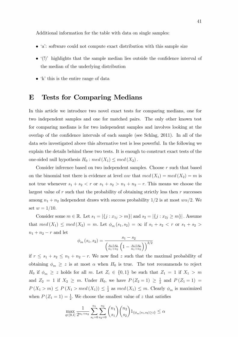
Additional information for the table with data on single samples:

� �a�: software could not compute exact distribution with this sample size

� �(!)� highlights that the sample median lies outside the con�dence interval ofthe median of the underlying distribution

� �k�this is the entire range of data

E Tests for Comparing Medians

In this article we introduce two novel exact tests for comparing medians, one for

two independent samples and one for matched pairs. The only other known test

for comparing medians is for two independent samples and involves looking at the

overlap of the con�dence intervals of each sample (see Schlag, 2011). In all of the

data sets investigated above this alternative test is less powerful. In the following we

explain the details behind these two tests. It is enough to construct exact tests of the

one-sided null hypothesis H0 : med (X1) � med (X2) :

Consider inference based on two independent samples. Choose r such that based

on the binomial test there is evidence at level �w that med (X1) = med (X2) = m is

not true whenever s1 + s2 < r or s1 + s2 > n1 + n2 � r: This means we choose thelargest value of r such that the probability of obtaining strictly less then r successes

among n1 + n2 independent draws with success probability 1=2 is at most w�=2: We

set w = 1=10:

Consider some m 2 R. Let s1 = jfj : x1j > mgj and s2 = jfj : x2j � mgj : Assumethat med (X1) � med (X2) = m: Let �m (s1; s2) = 1 if s1 + s2 < r or s1 + s2 >

n1 + n2 � r and let�m (s1; s2) =

s1 � s2�s1+s2n1+n2

�1� s1+s2

n1+n2

��3=2if r � s1 + s2 � n1 + n2 � r: We now �nd z such that the maximal probability ofobtaining �m � z is at most � when H0 is true. The test recommends to reject

H0 if �m � z holds for all m: Let Zi 2 f0; 1g be such that Z1 = 1 if X1 > m

and Z2 = 1 if X2 � m: Under H0; we have P (Z2 = 1) � 12and P (Z1 = 1) =

P (X1 > m) � P (X1 > med (X1)) � 12as med (X1) � m: Clearly �m is maximized

when P (Z1 = 1) = 12: We choose the smallest value of z that satis�es

maxq2[0;1]

1

2n1+n2

n1Xs1=0

n2Xs2=0

�n1s1

��n2s2

�1f�m(s1;s2)�zg � �

42

where 1f�g is the indicator function.

We now prove that the rejection probability is bounded above by � when H0 is

true. Clearly this is the case when P (X2 � med (X2)) =12: Assume that

P (X2 � med (X2)) >12: Then there exists an independent random variable Q 2

f0; 1g such that P (X2 � med (X2) ; Q = 1) =12: It is as if each of the realizations

of X2 = med (X2) have a label Q. Assume that Q is observable each time X2 is

observable. Replace Z2 above by Z 02 2 f0; 1g de�ned by Z 02 = 1 if X2 � m and Q = 1

and replace s2 by s02 = jfj : x2j � m; qj = 1gj : Then P (Z 02 = 1) = 1=2 under H0 andthe rejection probability of the above test is bounded above by �: Note that s02 � s2:If we then replace back s02 by s2 then the test statistic gets smaller and we reject less

often, in particular the rejection probability is bounded above by �: But if we replace

s02 by s2 then we do not need to observe Q and the proof is complete.

The test for matched pairs is very similar to the one for independent samples.

Choose r such that the probability of obtaining strictly less than r successes among

n independent draws with success probability 12is at most w�=2 where w = 1=10:

Consider again somem 2 R. Let b = jfj : x1j > m > x2jgj, c = jfj : x1j � m � x2jgjand d = jfj : x1j > m; x2j � mgj : Assume that med (X1) � med (X2) = m: Let

�m (b; c) =1 if b+ c+ 2d < r or if b+ c+ 2d > 2n� r; for r � b+ c+ 2d � 2n� rlet �m (b; c) =

b�cpb+c

if b + c > 0 and �m (0; 0) = 0: We choose z such that the maxi-

mal probability of obtaining �m � z is at most � when H0 is true. Let Z 2 f0; 1g2

such that Zi = 1 if and only if Xi � m: Under H0; we have P (Z2 = 1) � 12and

P (Z1 = 1) = P (X1 > m) � P (X1 > med (X1)) � 12as med (X1) � m: Clearly �m

is maximized when P (Z1 = 1) = 12: Let q = P (Z = (1; 0)) : Then P (Z = (0; 1)) = q

and P (Z = (1; 1)) = 12� q when P (Z2 = 1) = 1

2. We choose the smallest z such that

maxq2[0;1]

nXb=0

n�bXc=0

n�b�cXd=0

n!

b!c! (n� b� c� d)!qb+c

�1

2� q�n�b�c

1f�m(b;c)�zg � �:

It follows, using analogous arguments as in the case of independent samples, that the

rejection probability of the test is bounded above by � when H0 is true.

The above tests for two independent samples and matched pairs are easily general-

ized to be able to consider H0 : med (X1) = m1;med (X2) = m2 for all (m1;m2) 2 R2

and thus to construct con�dence intervals for med (X1)�med (X2) :

43

F Software

All software is available in R. We used the implementations of the Wilcoxon-Mann-

Whitney and Wilcoxon tests available in the R package �coin�. For the robust rank

order test we took the test statistic from the R package �NSM3�and critical values

from Feltovich (2005) which are only available for ni � 40. For the test of stochasticinequality of Brunner and Munzel (2000) we used the R package �lawstat�. Software

for the tests for stochastic inequality, equality of means (for small and moderate

sample sizes) and for the mean of a single sample are contained in the R package

�npExact�that can be found at https://github.com/zauster/npExact.git. The equal-

ity of means test for large sample sizes and the two tests for comparing medians

are available at https://homepage.univie.ac.at/karl.schlag/. The median di¤erence

test is derived from the test for stochastic inequality as follows. We wish to test

H0 : med (X1 �X2) � d; which is equivalent to H0 : P (X1 � X2 + d) � 12which is

equivalent to H0 : P (X1 > X2 + d) � P (X1 � X2 + d) : Consider some " > 0 with

" < mini;j fx1i � x2j : x1i 6= x2jg and test H0 : P (X 01 > X

02) � P (X 0

1 < X02) ; setting

X 01 = X1 � " and X 0

2 = X2 + d. So we decreased X1 slightly so that there are

no more ties and so that x1i � x2j + d holds if and only if (x1i � ") < x2j + d.

To test H0 : med (X1 �X2) � d use the fact that this is equivalent to testing

H0 : med (X2 �X1) � �d: