who gets to look nice and who gets to play? effects of ... · of child gender on household...

Who gets to look nice and who gets to play? Effectsof child gender on household expenditures

Krzysztof Karbownik1 • Michal Myck2

Received: 2 March 2015 / Accepted: 24 February 2016 / Published online: 3 March 2016

� The Author(s) 2016. This article is published with open access at Springerlink.com

Abstract We examine the relationship between a child’s gender and family

expenditure using data from the Polish Household Budget Survey. Having a first-

born daughter as compared with a first-born son increases the level of household

expenditures on child and adult female clothing, and it reduces spending on games,

toys and hobbies. This could be a reflection of a pure gender bias on behalf of the

parents or a reflection of gender complementarities between parents’ and children’s

expenditures. We find no robust evidence on gender differences in educational

investment, measured by kindergarten expenditure. The analysed expenditure pat-

terns suggest a so-far unexamined role of gender in child development. Parents in

Poland seem to pay more attention to how girls look and favour boys with respect to

activities and play, which could have consequences in adult life and contribute to

sustaining gender inequalities and stereotypes.

Keywords Gender differences � Household expenditures � Early childhood

JEL Classification D12 � J13

& Michal Myck

[email protected]

Krzysztof Karbownik

[email protected]

1 Institute for Policy Research, Northwestern University, 2040 Sheridan Road, Evanston,

IL 60208, USA

2 Centre for Economic Analysis - CenEA, ul. Krolowej Korony Polskiej 25, 70-486 Szczecin,

Poland

123

Rev Econ Household (2017) 15:925–944

DOI 10.1007/s11150-016-9328-y

http://crossmark.crossref.org/dialog/?doi=10.1007/s11150-016-9328-y&domain=pdf

http://crossmark.crossref.org/dialog/?doi=10.1007/s11150-016-9328-y&domain=pdf

1 Introduction

Children’s gender has been demonstrated to influence family stability (Dahl and

Moretti 2008), fertility (Ben-Porath and Welch 1976; Das 1987), abortion rates (Sen

1990; Jha et al. 2006), investment in nutrition and child care (Behrman 1988;

Jayachandran and Kuziemko 2011; Barcellos et al. 2012), household expenditure

(Lundberg and Rose 2004), educational and behavioural outcomes (Bertrand and

Pan 2013, Autor et al. 2015), voting preferences (Oswald and Powdthavee 2010)

and labour market activity (Lundberg and Rose 2002; Ichino et al. 2013).1 These

effects are sometimes explained by gender-biased preferences of parents who, for

example, would rather have a boy than a girl. On a number of outcomes, however,

they are also consistent with gender-neutral preferences. In these instances, they

refer to differences in costs of bringing up boys and girls, differences in the returns

from investment in the child’s human capital (especially prevalent in the developing

world) and the importance of gender-specific roles in the upbringing process. In

some cases, such as the effect on voting behaviour, the most natural explanation is a

direct causal consequence of children’s gender on changes in parental preferences.2

Using a detailed dataset on expenditures of Polish households, we extend the

existing pool of evidence on the effects of children’s gender to include its role in

changing household consumption behaviour. Focusing on expenditure patterns may

provide further clues in understanding the mechanisms behind the already-identified

effects on parental outcomes. If there is differential treatment of boys and girls by

their parents, then it should be reflected in the way households allocate their

resources, which is of particular importance in the light of the growing evidence on

the role of early interventions (Blau and Currie 2006; Cascio 2009; Almond and

Currie 2011; Carneiro and Ginja 2014) and investment in children in the form of

prenatal care, vaccinations or medical care (Aizer 2003; Figlio et al. 2009; Levine

and Schanzenbach 2009). Thus, differential levels of expenditure related to the

child’s human capital development or on items that may solidify gender stereotypes

could have long-term consequences for children’s outcomes in the future.

The Polish Household Budget Survey (PHBS), which we use in this paper, offers

a unique chance to study detailed patterns of household expenditures differentiated

by a child’s gender as well as other family characteristics. In contrast to most

expenditure datasets, in the PHBS it is possible to classify a number of detailed

expenditures by age and gender. This allows us to split spending between adults and

children aged up to 12 and by gender among adults.3

1 For a review of economic, sociological and psychological studies, see Raley and Bianchi (2006).2 In Oswald and Powdthavee (2010), since children’s gender enters their father’s utility function, the

outcome—in this case, parental voting behavior—is conditional on the number of boys and girls.3 In the United States, the Consumer Expenditure Survey (CEX) also contains some information on

child-specific expenditure such as clothing and private education. In the US data, however, children’s

goods are classified up to the age of 17. This might be a problem because the older the children the more

they take an active part in consumption decisions. Therefore, in the US, we often cannot distinguish

between the decision of a teenager and that of a parent. Furthermore, CEX offers small sample sizes

relative to the US population. For example, Blundell et al. (2008) start off with 192,564 households for

years 1980 to 2004 but end up using only 14,430 households with complete data for their food demand

estimation; Charles et al. (2009) use 1986 to 2002 data for all households and work with a sample of

926 K. Karbownik, M. Myck

123

Using data for the years 2003–2011, in the main analysis we compare 14,893

married couples with first-born girls and 16,164 married couples with first-born

boys to study the differential patterns of household expenditure.4 Subsequently we

restrict the sample to families with two children of the same gender where we

compare households with two girls versus two boys.5 Since we observe some

families in two consecutive years, in total we work with the main sample of 46,185

observations and the two girls versus two boys sample of 9515 observations. We

first discuss three main potential confounding factors, namely marital stability,

fertility and labour supply. We then examine the effect of child’s gender on total

expenditure, adult clothing expenditure (Lundberg and Rose 2004) and child-related

expenditure items, such as spending on clothing for children aged below 13 and

expenditure on kindergarten. Additionally, we examine two categories of expen-

diture that include mainly child-related goods, namely ‘games, toys and hobbies’

and ‘educational books and materials’.

We confirm that having a first-born girl decreases marital stability and fertility,

but we do not find any relationship between child’s gender and parental labour

supply. Our findings suggest that the gender of children can have a significant effect

on household expenditure patterns. We find that having a first-born girl increases

spending on clothing and shoes by 3.6 %, and this overall effect is found to reflect a

7.2 % increase in spending on women’s clothing, a 5.8 % decrease on men’s

clothing and a 6.0 % increase on children’s clothing (in all cases in the text when we

refer to clothing, the category also includes shoes expenditure). Moreover,

households with a first-born girl spend less on games, toys and hobbies (by

13.4 %). We show that expenditure data can also be used to examine differential

investment in human capital of sons and daughters. For example we find some

suggestive yet not definitive evidence that spending on kindergarten in Poland is

lower for girls. Overall the findings seem to point towards a gender-stereotypical

pattern of child-related expenditure rather than deliberate differential investment in

childhood human capital, with girls’ parents buying them more clothing and boys’

Footnote 3 continued

49,363 households. Lundberg and Rose (2004) use a sample of approximately 2400 families for years

1990 to 1998. Another problem in the case of the US is the much more lenient abortion legislation and

evidence that immigrants from Asia keep their skewed gender preferences towards boys even long after

immigration to North America (Almond et al. 2013). From this perspective, Poland offers a higher-quality

and larger dataset, homogeneous population, strict abortion legislation and only limited access to in vitro

fertilization (IVF) treatment. It is thus unlikely that our estimates will be biased due to lack of randomness

in the gender of a child.4 The descriptive statistics presented in Tables 1 and 2 document that the sample of married couples does

not differ substantially from the population of all families. We further explain reasons for the sample

selection in Sect. 4. We have also examined the relationship for the full population and for non-married

individuals (mostly single mothers). Our results are unchanged qualitatively in the sample of all

households and are often larger but statistically insignificant due to smaller sample sizes for non-married

households. These additional analyses are available in Karbownik and Myck (2015).5 If the gender of the first child affects family arrangements and fertility then focusing on the sample of

households with two children can lead to sample selection bias. We discuss this possibility in Sect. 4. In

the married sample with two children we observe 3002, families with two girls, 3539 families with two

boys and 6554 mix-gender families. We do not use the mixed gender families in the estimation but the

results are robust to including this set of households.

Who gets to look nice and who gets to play? Effects of… 927

123

Table 1 Descriptive statistics—demographics and labour market information

All families Married couples

Mean Girl–boy difference Mean Girl–boy difference

Living without a father 0.090

(0.286)

0.004

(0.002)

– –

Having never been married 0.046

(0.210)

0.004

(0.002)

– –

Separated or divorced 0.044

(0.205)

0.001

(0.002)

– –

Married 0.867

(0.340)

-0.006

(0.003)

1 –

Number of children 1.624

(0.760)

-0.005

(0.007)

1.664

(0.765)

-0.004

(0.007)

First-born girl 0.481

(0.500)

– 0.480

(0.500)

–

Age of mother 30.325

(4.560)

0.045

(0.040)

30.518

(4.427)

0.052

(0.041)

Age of mother at first birth 24.199

(3.874)

0.010

(0.034)

24.333

(3.800)

0.014

(0.035)

Mother’s educationa

Basic 0.342

(0.474)

-0.000

(0.004)

0.330

(0.470)

-0.003

(0.004)

Secondary 0.359

(0.480)

-0.004

(0.004)

0.360

(0.480)

-0.006

(0.004)

Higher 0.299

(0.458)

0.004

(0.004)

0.310

(0.463)

0.009

(0.004)

Mother works 0.605

(0.489)

0.003

(0.004)

0.616

(0.486)

0.002

(0.005)

Mother’s income (PLN) 692

(1020)

-10

(9)

696

(1021)

-8

(10)

Father works – – 0.93

(0.25)

0.000

(0.002)

Father’s income (PLN) – – 1673

(1646)

-6

(15)

Observations 53,300 46,185

Families 35,917 31,057

Notes The samples include families in which the mother is younger than 41 and older than 17 and had the

first child at the earliest at the age of 16; children’s age 0–12; expenditure information for households

with at most one family with children aged 0–12. Monetary values in Polish zloty (PLN) in June 2006

prices. Columns one and three provide means and standard deviations while columns two and four

provide differences between mean values for girls versus boys. Values in parentheses in even numbered

columns correspond to t test standard errors

Source Authors’ calculations based on PHBS data, 2003–2011a Education categories cover: basic—no formal education, primary education, gymnasium and vocational

education; secondary—secondary academic and secondary vocational education; higher education—

education degree higher than secondary


123

parents spending more on games. These findings naturally raise questions

concerning long-term consequences of such behaviour for the development of

boys and girls and their perception of social and gender roles.

The findings on clothing expenditure are consistent with a number of potential

hypotheses, and are in line with those already documented in the US for the total

clothing expenditure (Lundberg and Rose 2004). First of all, the gender of the first

child might have a direct effect on parents’ consumption preferences, which would

be in line with the effect of having a girl on voting preferences (Oswald and

Powdthavee 2010). Alternatively, mothers’ and daughters’ clothing might be

complements, in which case spending more on one may lead to higher spending on

the other, at the expense of fathers’ clothing.

Our findings constitute first evidence suggestive of the fact that a child’s gender

affects the patterns of both parental and child-related expenditure. On the one hand,

this evidence may reflect the direct effect of a child’s gender on parental

consumption preferences. On the other, it points towards a pattern of consumption

suggestive of early assignment of stereotypical gender roles. Thus, girls get to look

nice and boys get to play. Finally, we are also the first to study the relationship

between children gender and household behaviour in a post-communist country.

2 Data and sample statistics

We use a dataset from the Polish Household Budget Survey for years 2003–2011. It

is a nationally representative dataset collected annually by the Central Statistical

Office in Poland (GUS).6 The data include information on household demographic

composition and labour market activity, as well as income and expenditure data

recorded over the period of a month in which households participate in the survey.

In total, we have information on 323,754 households and 965,082 individuals over

the 9 years from 2003 to 2011. The PHBS contains a rolling panel element covering

over a third of the participating households, which are interviewed in two

consecutive years (in the same calendar month). In the full sample, we identify

121,382 households for which information is available for two periods.

Since the dataset does not contain retrospective fertility information, we rely only

on contemporaneous family composition. Individuals in every household are

matched into families, which we define as a single adult or a couple (married or

cohabiting) with any dependent children. This is done using available information

on the relationship to the head of household and detailed pairing in the data based on

the unique identifiers of mothers, fathers and partners of each individual. Following

other studies in the literature, we limit the analysis to mothers aged between 18 and

40 who had their first child at the earliest at the age of 16. The limit for the age of

the oldest child is set at 12 years, which is consistent with the approach of Dahl and

6 For more information on the methodology used by GUS see Barlik and Siwiak (2011). The

methodology complies with EUROSTAT recommendations. A summary of the survey methodology is

given in the ‘‘Appendix’’.


123

Moretti (2008) and at the same time corresponds to the grouping of expenditure

information on clothing.7

Because expenditure data are collected at the household level, we additionally

limit the sample to households where there is only one family with children below

13 years of age. This does not preclude the possibility of there being more than one

family in the household (for example, parents living with children and their

grandparents). In fact, such complex households are relatively common in Poland

(Haan and Myck 2012). In the full PHBS sample, 71.0 % of households contain

Table 2 Descriptive statistics—expenditure information

All families Married couples

Mean Girl–boy difference Mean Girl–boy difference

Panel A: gender-specific adult expenditure (average amounts, PLN)

Male 34.91

(108.02)

-2.23

(0.94)

38.07

(112.73)

-1.99

(1.05)

Female 63.01

(137.68)

3.66

(1.19)

63.54

(128.49)

4.99

(1.20)

Panel B: Child-related expenditure (average amounts, PLN)

Games and toys 21.22

(57.18)

-3.33

(0.5)

22.22

(58.75)

-3.04

(0.55)

Educational materials 19.42

(63.23)

1.07

(0.55)

19.98

(63.87)

0.92

(0.59)

Clothing and shoes 60.21

(90.46)

3.60

(0.78)

62.34

(92.29)

4.09

(0.86)

Kindergarten 29.82

(94.16)

-1.66

(0.82)

30.97

(96.35)

-1.44

(0.90)

Panel C: child-related expenditure (% with any positive expenditure)

Games and toys 0.41

(0.49)

-0.02

(0.00)

0.42

(0.49)

-0.02

(0.00)


(0.48)

0.02

(0.00)

0.35

(0.48)

0.02

(0.00)

Clothing and shoes 0.67

(0.47)

0.01

(0.00)

0.69

(0.46)

0.02

(0.00)

Kindergarten 0.15

(0.35)

-0.00

(0.00)

0.15

(0.36)

-0.00

(0.00)

Total declared expenditure: 2557.35 12.14 2629.92 23.11

(1949.61) (16.9) (1997.49) (18.60)


Families 35,917 31,057

Notes and source See Table 1

7 Sample selection bias is likely to be very small as schooling in Poland is compulsory until the age of 18

and most children live with their parents until at least that age.


123

only one family, 22.2 % include two and 6.8 % three or more. In the main sample

used in this analysis, 77.9 % are single-family households.8 We further restrict the

sample to families with a mother present in the household and where the child-

mother relationship is clearly specified in the data. We exclude twins and triplets at

first birth, widowed mothers and lone fathers.9

The analysis is conducted, for the most part, for the sample of married couples.10

If the welfare of families is affected by the marital status of parents, and the latter

driven to some extent by the gender of children, then any identified effect of gender

on expenditure in the full sample could be a consequence of different partnership

arrangements of girls’ and boys’ families, rather than directly a consequence of

different expenditure behaviour of boys’ and girls’ parents. Section 4 also presents

analysis of other potential sources of bias, namely the indirect effects of gender

through fertility, parental labour supply or household income. Since we do not find a

strong evidence for fertility effects we also present the main estimates for the

sample of families with two children where both children are of the same gender.

This sample provides a robustness test to verify the magnitude of the estimated

effects.11 We chose the sample of married families for the main analysis based on

two key premises: one, we can observe father’s labour supply and expenditure on

both male and female adult clothing; two, the outcomes that we observe in the

married and the full sample are very similar.12

Descriptive statistics are presented in Table 1 separately for all families and for

married couples. The sample size for all families is 53,300 and for the married

couples, used in the main analysis, it is 46,185. Among all families, 9.0 % of

children live without a father. The fraction of families living without a father, in the

full sample, can be decomposed into 4.6 % of mothers who haven’t been married

and 4.4 % of mothers who are divorced or separated. The average number of

children in the full sample is 1.62 and it is lower than among married couples. As

we show in Sect. 4 this could be due to the small first-born girl effects on having

two or more children. At the same time, the demographic and socio-economic

characteristics of the mothers are similar in the sample of all families and married

8 All our results hold regardless of whether we control for multifamily household status or not.9 Lone fathers are defined as families in which mothers do not live with their children in the household.

Paternal custody is rare in Poland. In the full sample we only have 492 cases of lone fathers aged 18–40

(which is the age group considered for estimation) of whom 60 are widowers. For comparison there are

9773 lone mothers in the full sample (827 widows) in the same age group.10 Results for the full sample of families and separately for non-married families have been presented in

Karbownik and Myck (2015).11 If the endogenous fertility is of a lesser concern then, similar to Lundberg and Rose (2004), we could

also estimate the relationship between child’s gender and expenditure for families with only one child. In

this sample we know with much higher probability that particular child goods expenditure is directed

towards specific child. Our results do not change substantively for this sample.12 We recognize that focusing on married couples induces a potential selection bias but since the

consumption results for all families and married couples are qualitatively unchanged and the quantitative

differences are generally smaller in the latter sample we conclude that the bias is likely small and present

the more conservative estimates for married copules. Detailed estimates for all samples are available in

Karbownik and Myck (2015).


123

families. These characteristics are also similar in the sample with two children of

opposite gender.

The PHBS contains detailed information on over 400 specific household

expenditure items collected over a period of a month. These items are aggregated

into 11 basic broad categories of expenditures such as food, clothing, housing and

energy, health, education and transport. Additionally, the dataset separates spending

on such items as clothing and shoes into male and female adult (aged at least 13)

and child (aged under 13) expenditures.13 Moreover, the detailed categories allow us

to identify the following items (see Table 2):

• games, toys and hobbies (labelled as ‘Games and toys’);

• educational books and educational stationery (‘Educational materials’);

• kindergarten expenditure (‘Kindergarten’).

While the first two of these three categories could include spending on adult

goods (e.g. on sports or fishing equipment and on training or educational books

unrelated to children’s education), they are most likely to cover child-related

expenses.14 The last category is directly related to expenditure on children.15

Among all families and married families, 15 % of households declare expenditure

on kindergarten in the month of the survey; 67–69 % of families declare positive

expenditure on child clothing, with an average (unconditional) expenditure of about

60 PLN ($19) per month.16 Positive spending on games and toys is recorded in

about 41 % of the households, and about 34 % declare positive expenditure on

educational books and materials, with the average (unconditional) amounts spent on

each of these categories equal to around 20 PLN ($6) per month. Thus, married

families do not seem to depart a lot from full population in terms of expenditure

patterns. Columns two and four in Table 2 present our main ‘‘raw’’ results

documenting differences in spending on children clothing, adult clothing as well as

games and toys. The differences in spending on educational materials and

kindergarten are more modest. As expected the average expenditure is generally

13 The total clothing category contains adult (male and female) and child clothing and shoes as well as

several smaller items such as dyeing and cleaning.14 The average expenditures in these categories in families without children are less than 25 % of those

among the families in our sample.15 Our survey data also include information on schooling and tutoring expenditure. Given that primary

schooling is for the most part public in Poland and we focus on households with the oldest child below the

age of 13, the incidence of private schooling or tutoring is very low. About 10 and 1 % of households

declare any positive spending on schooling and tutoring, respectively. The nominal values are also very

small. We could not detect any significant gender differences in expenditure on either of these categories.

Furthermore, spending on kindergarten, as expected, is concentrated among children aged 3–6, for

example among families with one child that declare positive kindergarten spending 91.9 % of these

children are between 3 and 6 years old, 5.7 % are younger than three and 2.4 % are older than six. We

provide the estimates for the restricted sample of families with children who are age-eligible for

kindergarten in Table 7 (‘‘Appendix’’).16 All absolute values are given in Polish zloty (PLN) in June 2006 prices. The exchange rate between the

US dollar and the PLN on June 14, 2006 was $1 = 3.194 PLN (National Bank of Poland). For reference:

the gross monthly minimum and mean wages in Poland in 2006 were respectively 899.10 PLN (Ministry

of Labour and Social Policy) and 2477.23 PLN (Central Statistical Office).


123

higher once we focus on families with two children of the opposite sex. The gender

differences are also aggravated, and we formally document this in a regression

framework in Sect. 5.

3 Modelling the effect of children’s gender on household expenditures

Our identification strategy relies on treating the child’s gender at first birth as

randomly determined. While some doubts have been raised with respect to the

randomness of this outcome (Das Gupta 2005; Hesketh et al. 2005; Dahl and

Moretti 2008; Almond and Rossin-Slater 2013), there are institutional reasons to

believe that the random assignment is not confounded in the case of Poland. These

include principally a culturally homogenous society, strict abortion legislation and

very limited access to in vitro fertilization and other assisted reproductive

treatments.17 The assumption of gender randomness implies that any differences

that we observe in terms of household expenditure can be attributed to the gender of

the child. Since the higher-parity fertility might be affected by the gender of the first

child (see Table 4), the most common approach in the literature is to focus on the

gender of the first child, in which case the estimated model for each of the

expenditure categories takes the following form:

Eji ¼ ðFirst child girliÞ0a1 þ X0

1ia2 þ X02ia3 þ ei ð1Þ

where Eij is the expenditure of household i in expenditure group j, vector X1 contains

mother’s socio-demographic characteristics (mother’s age at first birth, cubic

polynomial in age, educational attainment indicators), while X2 includes town size

indicators and regional and year dummies.18 The First child girl indicator takes

value 1 if the first-born child was a girl and 0 if it was a boy. ei is the residual, which

is clustered at household level because some households are observed twice in our

data. Since we are interested in estimating the differences between a single female

birth and a single male birth, we exclude twin and triplet births at first pregnancy

from the sample. Equation (1) is estimated by ordinary least squares (OLS) in

levels, and in each case we also report the percent effect.19 Since our consumption

data are at the household level, especially in the case of endogenous subsequent

fertility, the estimated differences based on the first-born child could be compressed

among families with more than one child. Nonetheless, if the endogenous fertility

17 Poland has also very little immigration and in particular immigration from Asian countries where

couples are known to exhibit strong gender preferences (Almond et al. 2013).18 Maternal education and town size can be endogenous with respect to first child gender. First, when we

do not control for these, the results remain unchanged. Second, we directly tested in a regression

framework that a child’s gender is not related to these controls. Expenditure estimates have also been

produced controlling for fertility and they do not change qualitatively.19 We could also compare twin-girl with twin-boy births, but we do not have enough power to credibly

conduct such an analysis. Given that we observe some households multiple times, we have also estimated

random effects models and models where we only keep the first or the second interview for each

household. We present these results in Table 6 (‘‘Appendix’’). The conclusions remain qualitatively

unchanged.


123

effects are small we can also estimate the model using the sample of families with

two or more children specifying if the first two children are either girls or boys. If

the gender-stereotypical spending hypothesis is correct we would expect to see

larger differences among households with two kids of the same gender than among

all households with first-born girls versus boys.

As already noted above, our results should be interpreted with caution if there are

substantial effects of child’s gender on partnership stability, fertility or parents’

labour supply. For example, if a first-born boy increases the probability of

partnership stability, and this has a positive effect on family resources, then

expenditure levels in such families could be higher. This would show up in the

estimations as the effect of a first-born boy, but could reflect only the indirect effect

of higher resources among families with a first-born boys, and not the effect of

different expenditure patterns directly resulting from the gender of the first child.

We show that partnership stability and fertility are significantly related to the gender

of the first child in Poland, but parental labour supply is not. In most cases, however,

the estimates for all and married families are very close, and in our results section

we focus on the latter subsample in which we can analyse both maternal and

paternal outcomes. Due to small sample sizes, we cannot provide meaningful

inference in the case of unmarried mothers (Karbownik and Myck 2015).

4 Potential confounding factors: partnership stability, fertilityand labour supply

In this section we first address the potential confounding factors in our analysis

related to family structure, fertility and labour supply. This analysis also motivates

our sample selection for consumption estimates. Table 3 presents regression results

from the model specified in Eq. (1) for the probabilities of living without a father, of

the mother having never been married and of the mother being divorced or

separated conditional on having been married. A significant coefficient on the First

child girl variable has usually been interpreted in the literature as a reflection of

parents’ gender preferences through its effect on the stability of parental

partnership. Our results confirm the influence of the gender of the first-born child

on family structure. The first child being a girl increases the probability of children

living without a father by 5.8 % and of the mother having never been married by

10.0 %. Unlike previous studies, however, we do not find any significant or sizable

effects of first-born child gender on the probability of divorcing or separating

conditional on being ever married. This could potentially be a consequence of the

Polish legal system, in which it is much harder and more costly to obtain a divorce

than in countries such as the US or Sweden. At the same time, in the sample with

two boys and two girls we see large, but insignificant, estimates for the probability

of divorce or separation. The results suggest that the gender of a child can have a

detrimental effect on family stability through selection into marriage, and this could


123

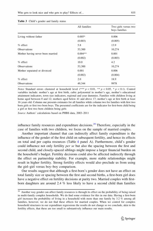
influence family resources and expenditure decisions.20 Therefore, especially in the

case of families with two children, we focus on the sample of married couples.

Another important channel that can indirectly affect family expenditure is the

influence of the gender of the first child on subsequent fertility, and hence its effects

on total and per capita resources (Table 4 panel A). Furthermore, child’s gender

could influence not only fertility per se but also the spacing between the first and

second child, and closely-spaced siblings might impose a larger financial burden on

the household’s budget. Fertility decisions could also be affected indirectly through

the effect on partnership stability. For example, more stable relationships might

result in higher fertility. Strong fertility effects would also preclude us from using

the girl–girl versus boy–boy comparison.

Our results suggest that although a first-born’s gender does not have an effect on

total family size or spacing between the first and second births, a first-born girl does

have a negative effect on fertility decisions at parity two. Married couples with first-

born daughters are around 2.4 % less likely to have a second child than families

Table 3 Child’s gender and family status

All families Two girls versus two

boys families

Living without father 0.005*

(0.003)

0.006

(0.005)

% effect 5.8 13.9


Mother having never been married 0.004**

(0.002)

0.001

(0.003)

% effect 10.0 4.2


Mother separated or divorced 0.001

(0.002)

0.006

(0.004)

% effect 2.0 18.9

Observations 49,344 9978

Notes Standard errors clustered at household level (*** p\ 0.01, ** p\ 0.05, * p\ 0.1). Control

variables include: mother’s age at first birth, cubic polynomial in mother’s age, mother’s educational

attainment indicators, town size indicators, regional and year dummies. Families with children living at

home aged between 0 and 12; mothers aged below 41 and above 17; mother’s age at first birth at least

16 years old. Column one presents estimates for all families while column two for families with first two

born girls or first two born boys. The presented coefficients are for the indicator for first-born child being

a girl or first two born children being girls

Source Authors’ calculations based on PHBS data, 2003–2011

20 Another way gender can affect family resources is through its effect on the probability of being raised

in multi-family complex households. We do find some evidence for this in our data. Having a first-born

girl increases the probability of living in a household with more than one family by 3.2 % among all

families, however, we do not find these effects for married couples. When we control for complex

household structures in our expenditure regressions the results do not change so we conclude, akin to the

fertility effects, that these are too small to substantively influence our main results.


123

with first-born sons. We do not find any statistically significant or economically

meaningful evidence that gender affects fertility at any other parity margin and,

given the fact that controlling for fertility does not alter our consumption estimates,

we conclude that these relatively small effects should not substantially bias our

main estimates. Because the fertility effect sizes are relatively small we present the

consumption estimates also for families with first two girls versus first two boys,

however, we treat these estimates with caution as gender of the child can be

assumed, conditional on cultural and institutional caveats, to be purely random only

in the case of the first birth. It is notable, though, that the negative coefficient on

Table 4 Effect of child’s gender on fertility, labour supply and income among married couples

All 0–2 Two girls versus two boys families

Panel A: family fertility

Total number of children -0.007

(0.008)

– –

% effect -0.4

Two or more children -0.012**

(0.005)

– –

% effect -2.4

Time between first two births -0.067

(0.041)

– –

% effect -0.1

Observations 46,185

Panel B: mothers’/households’ labour supply

P(working) -0.003

(0.005)

-0.004

(0.010)

0.007

(0.011)

% effect -0.4 -0.8 1.1

Income from work -15.060

(9.626)

-14.703

(22.022)

-13.540

(21.699)

% effect -2.1 -2.3 -2.0

Disposable income -42.868

(27.926)

-36.784

(51.404)

-92.615

(84.643)

% effect -1.3 -1.1 -2.8

Observations 46,185 9945 9515

Panel C: fathers’ labour supply

P(working) -0.000

(0.003)

0.003

(0.005)

0.000

(0.006)

% effect -0.1 0.3 0.0

Income from work -8.483

(16.054)

-58.362*

(30.900)

30.996

(36.059)

% effect -0.5 -3.3 1.8

Observations 46,185 9945 9515

Notes and source See Table 3. The ‘‘0–2’’ sample restricts the age of the oldest child to be lower or equal

to two. Monetary values in Polish zloty (PLN) in June 2006 prices


123

First child girl in the fertility equation points towards girl preferences, which seems

to contradict our family stability findings. In this case, however, lower fertility could

be driven by sample selection bias related to partnership stability.

Results in panels B and C show the effect of children’s gender on parental

employment, labour market income as well as on total household disposable

income. The sample focuses on married mothers and their husbands but the results

are very similar in the full population.21 The first column presents estimates for

maximum number of families, the second column intends to uncover the direct

effect of gender on outcomes that are independent from fertility by focusing on

households where the oldest child is between 0 and 2 years old, while the third

column displays estimates from the sample where we compare girl-girl to boy-boy

families.22 In panel B we report results for mothers or households, and in panel C

for labour supply of fathers. With the exception of a marginally significant effect on

paternal labour income among families with oldest child between 0 and 2, we do not

find any evidence that gender of the first-born child significantly affects any of the

labour market outcomes. The estimates are generally small in magnitude compared

with our consumption estimates and, if anything, they work in the opposite direction

to the effects found for advanced economies in Ichino et al. (2013). Thus, in the case

of Poland, we reject the hypothesis that the gender of a first-born child or first two

children matters significantly for parental labour supply or household resources as

proxied by disposable income.

5 Differential expenditure by gender

In this section, we present the main results (Table 5) from the model outlined in

Sect. 3 for various expenditure categories: total household consumption, child-

related goods as well as clothing spending for adults split by gender.23

In the case of the total household expenditures we do not find any meaningful

differences by either the gender of the first-born child or the first two children being

of the same gender. At the same time there are gender differences in spending on

clothing, and these are present for both children and adults. In particular, we can

decompose the 3.6 % increase in spending on clothing in families with first-born

girls into a 5.8 % reduction in adult male spending, a 7.2 % increase in adult female

21 Due to sample size limitations, we cannot credibly use widowhood as an exogenous shock to family

resources. Nonetheless, when we estimate the labour supply regressions for the main sample of 294

widows, we cannot confirm any significant effects of child’s gender on maternal labour supply.

Furthermore, to increase power, we also use the whole sample and interact widowhood with first-born’s

gender. In this specification, we do not find any significant or sizable effects of either the gender dummy

or the interaction term.22 Arguably majority of mothers with children age 0–2 would not decide to have another child, and

because of this we cannot estimate the comparison between two girls and two boys in this sample.23 In the previous version of this paper (Karbownik and Myck 2015) we also presented the estimates for

11 broad expenditure categories e.g. food or services or durables. This is akin to the exercise in Lundberg

and Rose (2004) and similarly to them, in majority of cases we did not observe any meaningful or

statistically significant differences by gender of the first child. In the case of food and communication

expenditures we detected statistically significant but not economically meaningful differences.


123

spending and a 6.0 % increase in child spending. These differentials are aggravated

for the sample of families with two children of the same gender.24 This suggests that

either there is a direct effect of child’s gender on parental consumption preferences

or there is a degree of complementarity between mothers’ and daughters’ clothing

consumption that is also reflected in the reduction of spending on adult male

clothing.

Among the analysed child-related expenditures other than clothing, we also find

precisely estimated effects of the first-born’s gender on other items of spending. On

the intensive margin, these include ‘games and toys’ expenditure, which is lower

among households with first-born girls by 13.4 %. On the extensive margin,

households with first-born girls are less likely to declare expenditure within this

category by 4.2 %. The differences for families with two children of the same

gender are about twice the size in comparison to all families confirming our

hypothesis of aggravated differentials in the sample with more extreme gender

contrast. We also find that parents of first-born girls more frequently declare

expenditure on ‘educational materials’. At first, this seems contradictory to our

results on games and toys; however, when we split this category into educational

books and stationery, we find positive, substantive and significant coefficients only

for the latter category. This suggests that families may have a lot of very small

expenditures on educational stationery, such as pencils and crayons, which are

skewed towards girls. This is further confirmed by moderate decrease in the

estimated extensive margin effect between all families and families with either two

girls or two boys, suggesting that some of these purchases could be transferable

across children.

Finally, we find 5.1 % reduction in kindergarten expenditures for households

with first-born girls, which although marginally statistically insignificant (p value

0.105), is economically meaningful. These negative effects do not hold for the

sample where we compare two girls to two boys. However, as we demonstrate in the

‘‘Appendix’’, this is because expenditure on kindergarten is strongly determined by

the age of children as it can be positive only in households with children of eligible

age. Table 7 in ‘‘Appendix’’ provides estimates taking into account presence of

children in the relevant age range (3–6 years old), as well as their number and

gender.25 Due to lack of statistical power our conclusions regarding kindergarten

expenditure are not as strong as in the case of clothing or games and toys. The point

estimates for households with one eligible girl (the dummy for a girl) are negative

but insignificant in three out of four cases, and they seem to be driving the negative

24 We chose families with exactly two children and both of the same gender for our analysis at parity two

because this in our opinion provides the cleanest gender contrast. As a robustness check we also

investigated the effects in three additional samples. First, sample of more than two children where we

maintain the current treatment of two boys versus two girls. Second, sample with two children where we

include mixed gender siblings. Third, sample of more than two children where we include all gender

compositions and where the treatment is indicator for two girls. Our results do not change substantively in

these samples, and as expected, in terms of magnitude they fall in between the comparison of first-born

girl effects from the full sample and first two born girls effects from the sample of two girls and two boys.25 Detailed investigation of kindergarten expenditure suggests that among married families with two

children of the same gender 71 % declare positive spending if at least one of the children is aged three to

six.


123

coefficient found in Table 5. In the case of two eligible children expenditure on

kindergarten is more likely to be observed (the ‘‘both eligible’’ dummy) but the

signs are inconsistent across the gender compositions.

We have also investigated whether the differentiated pattern of expenditure

documented thus far is aggravated in families with lower socio-economic status

based on maternal education.26 We do not find much support for this hypothesis

with relatively similar spending on games and toys, however, the degree of

complementarity between mother and first-born daughter spending on clothing (and

substitutability with father’s spending) is higher among more affluent families. This

may be related to higher incomes and greater potential to treat clothing as luxury

spending beyond the necessary expenditures in these families.

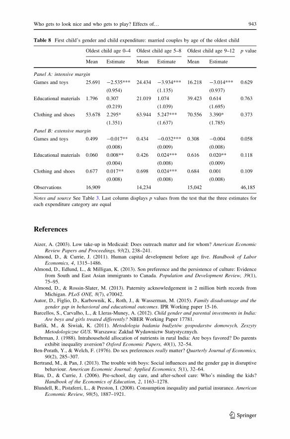
Results are also presented separately by subsamples defined by the age of the

oldest child (Table 8 in ‘‘Appendix’’), and older kids might express preferences

towards particular items and influence households’ expenditure patterns. We

therefore split the data into families where the oldest child is either 0–4 or 5–8 or

9–12 years of age. The estimates of gender differentials seem to reflect a u-shape

pattern in games and toys, clothing and educational materials, with the largest

gender differentials in expenditure for children aged 5–8. These differences

Table 5 Child’s gender and child expenditure among married couples

Married families with one or more

children

Married two children families: BB versus

GG families

Intensive

margin

%

effect

Extensive

margin

%

effect

Intensive

margin

%

effect

Extensive

margin

%

effect

Total

household

consumption

11.860

(19.272)

0.5 – – 35.437

(47.930)

1.3 – –

Games and

toys

-3.177***

(0.593)

-13.4 -0.018***

(0.005)

-4.2 -6.254***

(1.361)

-25.0 -0.039***

(0.011)

-9.3

Educational

materials

0.718

(0.658)

3.7 0.018***

(0.004)

5.1 1.710

(1.572)

7.0 0.017*

(0.010)

3.9

Children

clothing

3.610***

(0.931)

6.0 0.014***

(0.005)

2.1 10.592***

(2.364)

15.8 0.034***

(0.010)

4.9

Kindergarten -1.603

(0.990)

-5.1 -0.005

(0.004)

-3.0 1.693

(2.657)

4.4 -0.006

(0.009)

-3.4

Adult male

clothing

-2.285**

(1.064)

-5.8 -0.017***

(0.005)

-4.0 -2.008

(2.417)

-5.4 -0.020*

(0.011)

-4.9

Adult female

clothing

4.403***

(1.286)

7.2 0.018***

(0.005)

3.0 9.046***

(3.116)

15.5 0.037***

(0.011)

6.4

Observations 46,185 9515

Notes and source See Table 3. BB is two boys and GG is two girls families. Monetary values in Polish

zloty (PLN) in June 2006 prices

26 These results are available in Karbownik and Myck (2015).


123

however, in most cases, are not statistically significant due to relatively small

sample sizes.

6 Conclusion

Gender of children has been shown to influence their parents’ decisions in many

important dimensions. There is also ample evidence from the developing countries

that parents treat boys and girls differently when it comes to human capital

investment. In both cases, the mechanisms believed to be responsible for parental

decisions involve either biased preferences against one gender or an optimization

mechanism reflecting different costs of investment in boys and girls or different

returns from these investments. Some of the findings presented in this paper can also

be explained within these frameworks. Parents may be biased against girls when it

comes to expenditure on games, toys and hobbies (on average 13.4 %) and against

boys when it comes to expenditure on children’s clothing and shoes (6.0 %). They

may also differentiate expenditure on boys and girls because they believe that there

are different returns from such ‘investments’. In our view, however, some of our

results are difficult to square with these explanations and should rather be attributed

to a direct effect of children’s gender on parental preferences. For example, the fact

that parents with first-born girls spend more on adult female and child clothing and

less on adult male clothing than households with first-born boys is hard to reconcile

with any of the above explanations using either gender-biased or gender-neutral

preferences.27

Differentiated spending on clothing and toys by child’s gender, which could be

thought of as gender stereotypical, could suggest a so-far unexamined role of gender

in child development. The data suggest that while parents focus more on boys’

activities, they pay more attention to how girls look, which is reflected in the

expenditure on clothes. Expenditure data may also be informative on more direct

forms of human capital investment such as spending on kindergarten. While the

evidence in the PHBS in this regard is inconclusive we find some indication that

parental investment decisions take gender of their kids into account, and although

our estimates lack statistical power, they generally suggest that spending on girls is

lower. If parents invest less in girls in this regard, this could potentially have

important future consequences for the welfare of these children (Blau and Currie

2006). While we do not know what happens to these children later in adolescence

and adulthood, the differentiated expenditure patterns we document could have

consequences in adult life and contribute to sustaining gender inequalities.

Acknowledgments Data used in this paper come from the Polish Household Budget Survey

(2003–2011) collected annually by the Polish Central Statistical Office (GUS). GUS takes no

responsibility for the results and conclusions presented in this paper. We are grateful to Maja Adena,

Per-Anders Edin, David Figlio, Rita Ginja, Jonathan Guryan, Hans Gronqvist, Mikael Lindahl, Bjorn

Ockert and Erik Plug for valuable comments and suggestions, and to Judith Payne and Monika

27 As in Oswald and Powdthavee (2010), this would not have to imply a different utility function, but

only conditionality of marginal utilities on the gender of children.


123

Oczkowska for careful proofreading of the final manuscript. We are very grateful to two anonymous

referees for comments on the early version of the paper. The article is part of a research project financed

by the Polish National Science Centre (2012/05/B/HS4/01417), the support of which is gratefully

acknowledged.

Open Access This article is distributed under the terms of the Creative Commons Attribution 4.0

International License (http://creativecommons.org/licenses/by/4.0/), which permits unrestricted use, dis-

tribution, and reproduction in any medium, provided you give appropriate credit to the original

author(s) and the source, provide a link to the Creative Commons license, and indicate if changes were

made.

Appendix

Polish Household Budget Survey: summary of the methodology

The Polish Household Budget Survey is a representative survey of Polish

households. It is conducted every year and is spread over the entire calendar year,

with each household surveyed over a period of a month during which it records its

expenditures and incomes. This information is complemented with an additional

interview, which is conducted at the end of each quarter of data collection (the so-

called quarterly interview). Each year since 2005, when the most recent sampling

procedure was introduced, the target sample is 37,584 households.

In the case of refusal to participate among households from the principal gross

sample, households are replaced by another household from a reserve list of

randomly-chosen households. This reserve list is prepared separately for each

sampling unit. Households that drop out of the survey in the first half of their survey

month are also replaced by households from the reserve list. Those that drop out in

the second half of the month are not replaced. Households from the principal gross

sample that agree to participate are re-interviewed in the same month of the

following year. Households from the reserve list are not re-interviewed. The survey

methodology has been developed in accordance with the EUROSTAT guidelines.

The overall response rate in the survey in 2010 was 50.2 %. Survey non-response

was due to refusal to participate (48.1 %), survey dropout during its duration

(1.6 %) or refusal to complete the final quarterly interview (0.1 %).


123

http://creativecommons.org/licenses/by/4.0/

Table 7 Kindergarten expenditure: married couples

One or two children in the eligible age

range

One or two children in the eligible age

range and first eligible

Intensive margin Extensive margin Intensive margin Extensive margin

Both eligible 40.839***

(7.313)

0.057***

(0.019)

35.584***

(7.786)

0.014

(0.021)

Girl–Boy -2.490

(2.439)

-0.022***

(0.008)

-2.141

(3.644)

-0.016

(0.011)

Boy–Girl 0.206

(2.897)

-0.038***

(0.009)

0.039

(4.336)

-0.056***

(0.012)

Girl–Girl 0.224

(8.677)

0.007

(0.022)

-0.016

(8.876)

0.003

(0.023)

Girl -0.430

(8.480)

-0.031

(0.023)

-0.689

(8.881)

-0.042*

(0.024)

Mean of Y 61.55 0.30 69.67 0.33


Families 15,213 10,343

Notes and source See Table 3. Based on a sub-sample of households with one or two children who are

age-eligible for kindergarten (3–6 years old). Reference group for families with one child are families

where a boy is eligible, for those with two children—families with two boys who are age-eligible for

kindergarten

Table 6 First child’s gender and child expenditure among married couples

Margin All families Families interviewed twice

Random effects First interview Second interview

Intensive Extensive Intensive Extensive Intensive Extensive

Games and toys -3.239***

(0.592)

-0.018***

(0.005)

-2.934***

(0.660)

-0.018***

(0.006)

-4.072***

(0.709)

-0.022***

(0.006)

% effect -13.7 -4.3 -12.7 -4.3 -16.0 -5.1


(0.656)

0.016***

(0.004)

1.048

(0.712)

0.018***

(0.005)

0.807

(0.751)

0.014***

(0.005)

% effect 3.9 4.6 5.4 5.3 4.0 3.9

Clothing and shoes 3.767***

(0.929)

0.014***

(0.005)

4.488***

(1.055)

0.015***

(0.005)

3.769***

(1.079)

0.018***

(0.005)

% effect 6.2 2.1 7.5 2.2 6.1 2.7

Kindergarten -1.385

(0.973)

-0.004

(0.004)

-1.009

(1.067)

-0.003

(0.004)

-1.447

(1.143)

-0.003

(0.004)

% effect -4.5 -2.5 -3.2 -1.8 -4.3 -1.9

Observations 46,185 29,567 28,548

Notes and source See Table 3. Monetary values in Polish zloty (PLN) in June 2006 prices. Robust

standard errors in columns three to six


123

References

Aizer, A. (2003). Low take-up in Medicaid: Does outreach matter and for whom? American Economic

Review Papers and Proceedings, 93(2), 238–241.

Almond, D., & Currie, J. (2011). Human capital development before age five. Handbook of Labor

Economics, 4, 1315–1486.

Almond, D., Edlund, L., & Milligan, K. (2013). Son preference and the persistence of culture: Evidence

from South and East Asian immigrants to Canada. Population and Development Review, 39(1),

75–95.

Almond, D., & Rossin-Slater, M. (2013). Paternity acknowledgement in 2 million birth records from

Michigan. PLoS ONE, 8(7), e70042.

Autor, D., Figlio, D., Karbownik, K., Roth, J., & Wasserman, M. (2015). Family disadvantage and the

gender gap in behavioral and educational outcomes. IPR Working paper 15-16.

Barcellos, S., Carvalho, L., & Lleras-Muney, A. (2012). Child gender and parental investments in India:

Are boys and girls treated differently? NBER Working Paper 17781.

Barlik, M., & Siwiak, K. (2011). Metodologia badania bud_zetow gospodarstw domowych, Zeszyty

Metodologiczne GUS. Warszawa: Zakład Wydawnictw Statystycznych.

Behrman, J. (1988). Intrahousehold allocation of nutrients in rural India: Are boys favored? Do parents

exhibit inequality aversion? Oxford Economic Papers, 40(1), 32–54.

Ben-Porath, Y., & Welch, F. (1976). Do sex preferences really matter? Quarterly Journal of Economics,

90(2), 285–307.

Bertrand, M., & Pan, J. (2013). The trouble with boys: Social influences and the gender gap in disruptive

behaviour. American Economic Journal: Applied Economics, 5(1), 32–64.

Blau, D., & Currie, J. (2006). Pre-school, day care, and after-school care: Who’s minding the kids?

Handbook of the Economics of Education, 2, 1163–1278.

Blundell, R., Pistaferri, L., & Preston, I. (2008). Consumption inequality and partial insurance. American

Economic Review, 98(5), 1887–1921.

Table 8 First child’s gender and child expenditure: married couples by age of the oldest child

Oldest child age 0–4 Oldest child age 5–8 Oldest child age 9–12 p value

Mean Estimate Mean Estimate Mean Estimate

Panel A: intensive margin

Games and toys 25.691 -2.535***

(0.954)

24.434 -3.934***

(1.135)

16.218 -3.014***

(0.937)

0.629

Educational materials 1.796 0.307

(0.219)

21.019 1.074

(1.039)

39.423 0.614

(1.695)

0.763

Clothing and shoes 53.678 2.295*

(1.351)

63.944 5.247***

(1.637)

70.556 3.390*

(1.785)

0.373

Panel B: extensive margin

Games and toys 0.499 -0.017**

(0.008)

0.434 -0.032***

(0.009)

0.308 -0.004

(0.008)

0.058

Educational materials 0.060 0.008**

(0.004)

0.426 0.024***

(0.008)

0.616 0.020**

(0.009)

0.118

Clothing and shoes 0.677 0.017**

(0.008)

0.698 0.024***

(0.008)

0.684 0.001

(0.008)

0.109

Observations 16,909 14,234 15,042 46,185

Notes and source See Table 3. Last column displays p values from the test that the three estimates for

each expenditure category are equal


123

Carneiro, P., & Ginja, R. (2014). Long term impacts of compensatory preschool on health and behaviour:

Evidence from Head Start. American Economic Journal: Economic Policy, 6(4), 135–173.

Cascio, E. (2009). Do investments in universal early education pay off? Long-term effects of introducing

kindergartens into public schools. NBER Working Paper 14951.

Charles, K. K., Hurst, E., & Roussanov, N. (2009). Conspicuous consumption and race. Quarterly Journal

of Economics, 124(2), 425–467.

Dahl, G. B., & Moretti, E. (2008). The demand for sons. Review of Economic Studies, 75(4), 1085–1120.

Das, N. (1987). Sex preferences and fertility behaviour: A study of recent Indian data. Demography,

24(4), 517–530.

Das Gupta, M. (2005). Explaining Asia’s missing women: A new look at the data. Population and

Development Review, 31(3), 529–535.

Figlio, D., Hamersma, S., & Roth, J. (2009). Does prenatal WIC participation improve birth outcomes?

New evidence from Florida. Journal of Public Economics, 93(1–2), 235–245.

Haan, P., & Myck, M. (2012). Multi-family households in a labour supply model: a calibration method

with application to Poland. Applied Economics, 44(22), 2907–2919.

Hesketh, T., Liu, L., & Xing, Z. W. (2005). The effect of China’s one-child family policy after 25 years.

New England Journal of Medicine, 353(11), 1171–1176.

Ichino, A., Lindstrom, E.-A., & Viviano, E. (2013). Hidden consequences of a first-born boy for mothers.

Economics Letters, 123(3), 274–278.

Jayachandran, S., & Kuziemko, I. (2011). Why do mothers breastfeed girls less than boys? Evidence and

implications for child health in India. Quarterly Journal of Economics, 126(3), 1485–1538.

Jha, P., Kumar, R., Vasa, P., Dhingra, N., Thiruchelvam, D., & Moineddin, R. (2006). Low male-to-

female sex ratio of children born in India: National survey of 1.1 million households. Lancet,

367(9506), 211–218.

Karbownik, K., & Myck, M. (2015). Who gets to look nice and who gets to play? Effects of child gender

on household expenditure. IPR WP 15-03.

Levine, P.B., & Schanzenbach. D. (2009). The impact of children’s public health insurance expansions on

educational outcomes. NBER Working Paper 14671.

Lundberg, S., & Rose, E. (2002). The effects of sons and daughters on men’s labor supply and wages.

Review of Economics and Statistics, 84(2), 251–268.

Lundberg, S., & Rose, E. (2004). Investments in sons and daughters: Evidence from the consumer

expenditure survey. In: A. Kalil & T. DeLeire (Eds.), Family investments in children: Resources and

parenting behaviors that promote success (pp. 163–180). Mahwah, NJ: Lawrence Erlbaum

Associates.

Oswald, A. J., & Powdthavee, N. (2010). Daughters and left-wing voting. Review of Economics and

Statistics, 92(2), 213–227.

Raley, S., & Bianchi, S. (2006). Sons, daughters, and family processes: Does gender of children matter?

Annual Review of Sociology, 32, 401–421.

Sen, A. (1990). More than 100 million women are missing. New York Review of Books, 37(20), 61–66.


123

who gets to look nice and who gets to play? effects of ... · of child gender on household...

Documents