who benefits from government health spending … benefits from government health spending and why? a...
TRANSCRIPT
Policy Research Working Paper 7044
Who Benefits from Government Health Spending and Why?
A Global Assessment
Adam WagstaffMarcel Bilger
Leander R. BuismanCaryn Bredenkamp
Development Research GroupHuman Development and Public Services TeamSeptember 2014
WPS7044P
ublic
Dis
clos
ure
Aut
horiz
edP
ublic
Dis
clos
ure
Aut
horiz
edP
ublic
Dis
clos
ure
Aut
horiz
edP
ublic
Dis
clos
ure
Aut
horiz
edP
ublic
Dis
clos
ure
Aut
horiz
edP
ublic
Dis
clos
ure
Aut
horiz
edP
ublic
Dis
clos
ure
Aut
horiz
edP
ublic
Dis
clos
ure
Aut
horiz
ed

Produced by the Research Support Team
Abstract
The Policy Research Working Paper Series disseminates the findings of work in progress to encourage the exchange of ideas about development issues. An objective of the series is to get the findings out quickly, even if the presentations are less than fully polished. The papers carry the names of the authors and should be cited accordingly. The findings, interpretations, and conclusions expressed in this paper are entirely those of the authors. They do not necessarily represent the views of the International Bank for Reconstruction and Development/World Bank and its affiliated organizations, or those of the Executive Directors of the World Bank or the governments they represent.
Policy Research Working Paper 7044
This paper is a product of the Human Development and Public Services Team, Development Research Group. It is part of a larger effort by the World Bank to provide open access to its research and make a contribution to development policy discussions around the world. Policy Research Working Papers are also posted on the Web at http://econ.worldbank.org. The authors may be contacted at [email protected].
This paper uses a common household survey instrument and a common set of imputation assumptions to estimate the pro-poorness of government health expenditure (GHE) across 69 countries at all levels of income. Among the 66 countries for which the incidence of total GHE can be estimated, the mean and median concentration index values imply GHE is, on average, pro-rich. In only 26 countries, however, is the index statistically significant at the five percent level; in all but six of these, GHE is pro-rich. Gov-ernment health expenditure on contracted private facilities emerges as significantly pro-rich for all types of care, and in almost all Asian countries government health expen-diture overall is significantly pro-rich. The pro-poorness
of government health expenditure at the country level is significantly and positively correlated with gross domestic product per capita and government health expenditure per capita, significantly and negatively correlated with the share of government facility revenues coming from user fees, and significantly and positively correlated with six measures of the quality of a country’s governance; it is not, however, correlated with the size of the private sector nor with the degree to which the private sector delivers care dis-proportionately to the better-off. Because poorly-governed countries are underrepresented in the sample, government health expenditure is likely to be even more pro-rich in the world as a whole than it is in the countries in this study.

Who Benefits from Government Health Spending and Why? A Global Assessment
Adam Wagstaffa, Marcel Bilgerb, Leander R. Buismanc and Caryn Bredenkampd a Development Research Group, The World Bank, Washington DC, USA
b Signature Program in Health Services and Systems Research, Duke-NUS Graduate Medical School, Singapore
c Institute of Health Policy and Management, Erasmus University Rotterdam, Rotterdam, The Netherlands
d Health, Nutrition & Population Global Practice, The World Bank, Washington DC, USA
JEL Codes: H51, I14, I15
Acknowledgements
The research reported in this paper was partially supported by the World Bank’s Rapid Social Results Trust Fund (RSR). We are grateful to Nicole Klingen, Gayle Martin, Owen Smith, Aparnaa Somanathan, Owen O’Donnell, Ellen Van de Poel and Xiaoqing Yu for advice and useful comments on earlier versions of the paper, and to several World Bank regional staff for help identifying National Health Accounts data..

2
1. Introduction
A commonly stated reason why governments spend on the health sector, and
why donors supplement such spending in developing countries, is to reduce
inequalities in the distributions of health care utilization and health status
compared to what they would have been otherwise. Income redistribution may be a
second – although typically not explicit – objective: if there is limited scope to levy
income taxes, as is the case in many developing countries, a government may seek
to redistribute income by financing health care at a quality level that is just low
enough for the better off to decide to seek their health care privately (Besley and
Coate 1991). Yet despite the broad consensus that government health spending
(GHE) ought to disproportionately favor the poor, studies to date show that often
the reality is exactly the opposite.1
This literature is not, however, without its limitations. First, most studies
cover just one country or a few countries in a specific region; it is unclear therefore
how representative the results are of the world as a whole.2 Second, previous
studies have either worked with secondary tabulated survey data or (probably
better) have tried to harmonize ex post but often highly heterogeneous household
survey data; as a result it is unclear how comparable the results are across
1 BIA studies covering several countries include Castro-Leal et al. (1999; 2000), Filmer (2003), O’Donnell et al. (2007), Davoodi (2010). Mahal et al. (2001) report comparisons across India’s states. 2 There is only one previous multi-country benefit incidence analysis (BIA) study that has covered all regions of the world (Davoodi et al. 2010), which covers 56 countries. Others have focused on one region only: Castro-Leal et al. (1999; 2000) report results for a subset of African countries, while O’Donnell et al. (2007) report results for a subset of Asian economies.

3
countries.3 Third, there has been variation between and within studies in the
methods to impute subsidies at the individual level, even though it is known that
different methods are likely to produce different results; this makes it even less
clear how comparable the results are across studies and across countries within a
cross-country comparative study.4 Fourth, studies to date have paid scant attention
to the issue of sampling variability; few have presented confidence intervals around
their estimates of their indices of the pro-poorness of GHE.5 Fifth, few comparative
BIA studies go on to explore the issue of why countries vary in the degree to which
GHE is pro-poor; those that do explore a narrow subset of possible influences, and
none offers a coherent logical framework of the interrelationships between them.
In this paper we try to push the literature forward on all five fronts. First, we
present results for as many as 69 countries across all regions of the world.6 We
compare our 69 countries with the remaining countries of the world on variables we
find to be correlated with the pro-poorness of GHE in the WHS countries; based on
these differences and correlations, we extrapolate the incidence of GHE in the
countries we do not analyze. Second, our country estimates are based on microdata
drawn from a single household survey instrument that was implemented in the 69
countries; our country estimates are, therefore, we believe, highly comparable.
3 Davoodi et al. (2010) and Filmer (2003) work with tabulated data. Studies that try to harmonize ex post household survey data include O'Donnell et al. (2007) and Castro-Leal et al. (1999; 2000). 4 For example, O’Donnell et al. (2007) use the constant unit cost (CUC) assumption except in the case of India where they use the constant unit subsidy (CUS) assumption – these assumptions are explained below. 5 Only one other study to date (O'Donnell et al. 2007) has computed standard errors for estimates of GHE incidence. 6 The precise number of countries varies according to the analysis we do. We estimate the pro-poorness of overall GHE for 66 countries.

4
Third, we undertake cross-country comparisons only for countries for which we can
compute benefit incidence using the same method. This consistency is important
since it is known that the methods used to impute GHE at the individual level can
dramatically affect the conclusion of a BIA study, including the answer to the
fundamental question of whether spending disproportionately benefits the poor or
better off (Wagstaff 2012). We also explore how our results vary according to which
of three methods is used to impute subsidies at the individual level, and present
some new insights into the data requirements of each of the three methods. Fourth,
when comparing the incidence of GHE (using the concentration index) across
countries, including at the subsector level, we also report 95 percent confidence
intervals for the concentration index, which we obtain using bootstrapping. This
allows us to be sure that when a country appears to have a pro-poor or pro-rich
GHE distribution it is not due to sampling variability. Finally, we not only explore
more possible reasons why countries vary in the degree to which their GHE is pro-
poor, but we also suggest how they might fit together in a coherent logical
framework. Our evidence takes the form of cross-country correlations backed up
where possible by evidence on causality from the relevant literature.
The rest of the paper is organized as follows. Section 2 outlines the methods
we use both to measure the incidence of GHE at the country level and to
understand the sources of cross-country variation in the incidence of GHE. Section 3
outlines our data and discusses computation issues, again for both goals of the
paper. Section 4 presents our results, starting with the evidence on GHE incidence

5
at the country level and then moving to our results on the sources of cross-country
variation. Section 5 contains a discussion and section 6 our conclusions.
2. Methods
2.1 Measuring inequality in subsidy incidence
Suppose for the moment we can observe subsidies at the individual level.
Then we could measure the degree of inequality (by income or consumption) in
subsidies for subsector k, Sk, by computing the concentration index (CI) (Kakwani et
al. 1997). The CI for subsidies for subsector k, 𝐶𝐶𝐶𝐶𝑆𝑆𝑘𝑘, is derived from a Lorenz-type
plot of the cumulative share of the population ranked in ascending order of income
(or consumption) on the x-axis and the cumulative share of subsidies on the y-axis.
A negative (positive) value of the CI indicates a pro-poor (pro-rich) distribution (𝐶𝐶𝐶𝐶𝑆𝑆𝑘𝑘
is bounded by -1 and +1). Of course, the amount of subsidy individual i gets from
subsector k, Ski, is not observed in a household survey, and has to be imputed.
2.2 Computing the incidence of subsidies at the subsector level
At the individual level, subsidies received by individual i from subsector k are
equal to the difference between the costs incurred by the subsidy-receiving
providers used by individual i and the fees paid by individual i to these providers:
(1) 𝑆𝑆𝑘𝑘𝑘𝑘 = 𝐶𝐶𝑘𝑘𝑘𝑘 − 𝐹𝐹𝑘𝑘𝑘𝑘 = 𝑐𝑐𝑘𝑘𝑘𝑘𝑞𝑞𝑘𝑘𝑘𝑘 − 𝑓𝑓𝑘𝑘𝑘𝑘𝑞𝑞𝑘𝑘𝑘𝑘 = 𝑞𝑞𝑘𝑘𝑘𝑘(𝑐𝑐𝑘𝑘𝑘𝑘 − 𝑓𝑓𝑘𝑘𝑘𝑘) = 𝑞𝑞𝑘𝑘𝑘𝑘𝑠𝑠𝑘𝑘𝑘𝑘 .
Here, Cki, are the costs incurred by providers in subsector k in providing services to
individual i, Fki are the fees paid by individual i to providers in subsector k, qki is

6
the number of units of service of type k consumed by individual i, and cki, fki and ski
are the unit costs, fees and subsidies respectively for sector k for individual i. We
are likely to observe qki and fki in a household survey although in some surveys we
do not observe both. By contrast, we do not observe cki in a household survey, and
that is why imputation becomes necessary.
Three approaches to imputing subsidies at the individual level have been
proposed (Wagstaff 2012). The first is the “constant unit cost” (CUC) approach
which assumes that unit costs, cki, are constant across individuals and equal to ck.
In this case eqn (1) becomes
(2) 𝑆𝑆𝑘𝑘𝑘𝑘𝐶𝐶𝐶𝐶𝐶𝐶 = 𝑐𝑐𝑘𝑘𝑞𝑞𝑘𝑘𝑘𝑘 − 𝑓𝑓𝑘𝑘𝑘𝑘𝑞𝑞𝑘𝑘𝑘𝑘.
If data on the unit costs, ck, are available from administrative data or a health
facility survey, or have been estimated, and if individual-level data on the qki and fki
are also available in the household survey, 𝑆𝑆𝑘𝑘𝑘𝑘𝐶𝐶𝐶𝐶𝐶𝐶 can be computed at the individual
level, and the corresponding concentration index 𝐶𝐶𝐶𝐶𝑆𝑆𝑘𝑘𝐶𝐶𝐶𝐶𝐶𝐶 can be calculated.
Alternatively, as shown by Wagstaff (2012), 𝐶𝐶𝐶𝐶𝑆𝑆𝑘𝑘𝐶𝐶𝐶𝐶𝐶𝐶 can be computed as:
(3) 𝐶𝐶𝐶𝐶𝑆𝑆𝑘𝑘𝐶𝐶𝐶𝐶𝐶𝐶 = 𝐶𝐶𝑘𝑘
𝑆𝑆𝑘𝑘𝐶𝐶𝐶𝐶𝑞𝑞𝑘𝑘 −
𝐹𝐹𝑘𝑘𝑆𝑆𝑘𝑘𝐶𝐶𝐶𝐶𝐹𝐹𝑘𝑘,
where 𝐶𝐶𝐶𝐶𝑞𝑞𝑘𝑘 is the concentration index for utilization, 𝐶𝐶𝐶𝐶𝐹𝐹𝑘𝑘 is the concentration index
for fees, Fki, and Ck, Sk and Fk are aggregate costs, subsidies and fees respectively.
The shortcut in eqn (3) is useful when the country has a set of national health

7
accounts (NHA) that includes these aggregates: in this case, there is no need to get
the unit cost data for each of the subsectors.
A problem with the CUC assumption is that it is hard to rationalize why
people pay different amounts out-of-pocket for an outpatient visit or an inpatient
admission; the assumption implies that people paying more out-of-pocket get a
smaller subsidy.7 In reality it seems likely that higher fees reflect at least more
costly (and perhaps better quality) care, and that higher fees are not automatically
associated with a smaller subsidy. A second approach (the “constant unit subsidy”
or CUS assumption) which – unlike the CUC assumption – is consistent with this
idea assumes that the unit subsidy, ski, is constant across for a given subsector k. In
effect the government pays up to certain amount of the cost of care, and the user
pays each additional dollar of cost themselves out-of-pocket. Eqn (1) in this case
becomes (cf. Wagstaff 2012):
(4) 𝑆𝑆𝑘𝑘𝑘𝑘𝐶𝐶𝐶𝐶𝑆𝑆 = 𝑞𝑞𝑘𝑘𝑘𝑘𝑠𝑠𝑘𝑘 ,
so that subsidies for subsector k are proportional to utilization for subsector k. Thus
in this case, 𝐶𝐶𝐶𝐶𝑆𝑆𝑘𝑘 is simply equal to the CI for utilization (cf. Wagstaff 2012):
(5) 𝐶𝐶𝐶𝐶𝑆𝑆𝑘𝑘𝐶𝐶𝐶𝐶𝑆𝑆 = 𝐶𝐶𝐶𝐶𝑞𝑞𝑘𝑘.
Note that to compute 𝐶𝐶𝐶𝐶𝑆𝑆𝑘𝑘𝐶𝐶𝐶𝐶𝑆𝑆 we do not need to know the unit subsidy for subsector k,
sk. Nor do we need to know the cki and fki. Thus, not only is the assumption CUS
7 The CUC assumption is more plausible if there are means-tested subsidies that are effectively targeted.

8
arguably more plausible than the CUC assumption, it is also less demanding in
terms of data requirements.
A third approach (the “fees proportional to costs” assumption or FPC) is to
assume that unit costs and fees are proportional to one another.8 In this case, the
user pays a constant fraction of the cost of care, and the subsidy they receive is
proportional to the fees they pay. Under this assumption, the concentration index
for subsidies is therefore equal to the CI concentration index for fees (cf. Wagstaff
2012):
(6) 𝐶𝐶𝐶𝐶𝑆𝑆𝑘𝑘𝐹𝐹𝐹𝐹𝐶𝐶 = 𝐶𝐶𝐶𝐶𝐹𝐹𝑘𝑘.
Note that to compute 𝐶𝐶𝐶𝐶𝑆𝑆𝑘𝑘𝐹𝐹𝐹𝐹𝐶𝐶 all we need are the individual-level data on fees, fki, and
the variable used to rank individuals by their living standards.
The three approaches will give a different estimate of the extent to which
subsidies are pro-poor or pro-rich. In the plausible case where fees are more pro-rich
than utilization, Wagstaff (2012) has shown that the CUC assumption will lead to
the least pro-rich distribution of subsidies and the FPC assumption the most pro-
rich distribution; the CUS assumption falls somewhere in the middle. It is perfectly
possible that subsidies emerge as pro-poor under the CUC assumption but pro-rich
under the CUS and FPC assumptions.
8 The assumption of proportionality may be too strong; a weaker version proposed by Wagstaff (2012) – which we do not explore in this paper – is to assume that unit costs are a linear function of fees.

9
2.3 Computing the incidence of subsidies at the sector level
Whichever method is used to impute subsector-specific subsidies, we can
compute inequality in subsidies to the entire health sector as the concentration
index for total subsidies, 𝐶𝐶𝐶𝐶𝑆𝑆, which is equal to a weighted average of the
concentration indices for the various subsectors where the weight for subsector k is
equal to the subsector’s share in total subsidies. Thus, we have:
(7) 𝐶𝐶𝐶𝐶𝑆𝑆 = ∑ (𝑆𝑆𝑘𝑘 𝑆𝑆⁄ )𝐶𝐶𝐶𝐶𝑆𝑆𝑘𝑘𝑘𝑘 ,
where S is the amount of subsidy going to the entire health sector. In many
countries, a NHA is available containing data on S and with enough data to allow
the Sk to be estimated.9 When a NHA is not available, or when it does not include
sufficiently detailed information to allow the Sk to be estimated, the values of Sk
and their sum S can be estimated using microdata. We have:
(8) 𝑆𝑆𝑘𝑘 = ∑ 𝑐𝑐𝑘𝑘𝑘𝑘𝑞𝑞𝑘𝑘𝑘𝑘𝑘𝑘 − ∑ 𝑓𝑓𝑘𝑘𝑘𝑘𝑞𝑞𝑘𝑘𝑘𝑘𝑘𝑘
= ∑ 𝑞𝑞𝑘𝑘𝑘𝑘𝑘𝑘∑ 𝑐𝑐𝑘𝑘𝑘𝑘𝑞𝑞𝑘𝑘𝑘𝑘𝑘𝑘∑ 𝑞𝑞𝑘𝑘𝑘𝑘𝑘𝑘
− ∑ 𝑞𝑞𝑘𝑘𝑘𝑘𝑘𝑘∑ 𝑓𝑓𝑘𝑘𝑘𝑘𝑞𝑞𝑘𝑘𝑘𝑘𝑘𝑘∑ 𝑞𝑞𝑘𝑘𝑘𝑘𝑘𝑘
= 𝑄𝑄𝑘𝑘𝑐𝑐�̅�𝑘 − 𝑄𝑄𝑘𝑘𝑓𝑓�̅�𝑘 = 𝑄𝑄𝑘𝑘�𝑐𝑐�̅�𝑘 − 𝑓𝑓�̅�𝑘�,
where Qk is the total number of units of service of type k across the entire
population (e.g. the aggregate number of inpatient admissions), 𝑐𝑐�̅�𝑘 is the average
cost in the kth subsector per unit of utilization (e.g. per outpatient visit or per
inpatient admission), and 𝑓𝑓�̅�𝑘 is the average amount of fees paid in the kth subsector
per unit of utilization. We can compute Qk as:
9 Computing 𝐶𝐶𝐶𝐶𝑆𝑆𝑘𝑘𝐶𝐶𝐶𝐶𝐶𝐶 using eqn (3) requires such data to be available.

10
(9) 𝑄𝑄𝑘𝑘 = 𝑁𝑁 ∙ 𝑞𝑞�𝑘𝑘 ,
where N is the number of persons in the population, and 𝑞𝑞�𝑘𝑘 is the utilization rate
for subsector k (e.g. the number of inpatient admissions per capita); often it will be
possible to estimate the utilization rate from the household survey. Since what we
need for eqn (7) are the subsidy shares, the population size, N, cancels out, and we
have:
(10) 𝑆𝑆𝑘𝑘𝑆𝑆
= 𝑄𝑄𝑘𝑘(𝑐𝑐�̅�𝑘−�̅�𝑓𝑘𝑘)𝑄𝑄1(𝑐𝑐1̅−�̅�𝑓1)+𝑄𝑄1(𝑐𝑐2̅−�̅�𝑓2)+⋯+𝑄𝑄𝐾𝐾(𝑐𝑐�̅�𝐾−�̅�𝑓𝐾𝐾) = 𝑞𝑞�𝑘𝑘(𝑐𝑐�̅�𝑘−�̅�𝑓𝑘𝑘)
𝑞𝑞�1(𝑐𝑐1̅−�̅�𝑓1)+𝑞𝑞�2(𝑐𝑐2̅−�̅�𝑓2)+⋯+𝑞𝑞�𝐾𝐾(𝑐𝑐�̅�𝐾−�̅�𝑓𝐾𝐾).
Data on the average costs, 𝑐𝑐�̅�𝑘, would need to come from administrative data or from
a health facility survey, while data on the average fees, 𝑓𝑓�̅�𝑘, can be estimated from
the household survey.
2.4 Understanding the sources of cross-country variation in subsidy incidence
Once we have estimates of the pro-poorness of GHE at the country level, we
want to ask why some countries have more pro-poor distributions of GHE than
others.
O’Donnell et al. (2007) suggest several factors that may account for the
variation across countries in the pro-poorness of GHE. Richer countries, they argue,
are more likely to have pro-poor distributions of GHE since they will have the

11
resources to have a well-funded publicly-financed universal health system.10
O’Donnell et al. also suggest that countries with higher levels of GHE will have
more pro-poor (or less pro-rich) distributions of GHE. One explanation is that
higher levels of GHE “afford… a wider geographic distribution of public health
facilities and so bring services closer to poor, rural populations.” Another is that the
better off capture the initial dollars of GHE, but as spending increases and the
needs of the better off decline, spending becomes more pro-poor. Finally, O’Donnell
et al. suggest that the pro-poorness of GHE will be higher the bigger the quality gap
between government services and private-sector alternatives, since the larger this
gap the more likely it is that the better off will opt out of the public system;
however, they do not test this hypothesis due to lack of data on quality.
The 2004 World Development Report (WDR) (World Bank 2003) sheds
additional light on both the proximate and underlying causes of a pro-rich
distribution of GHE. Governments often emphasize in their resource-allocation
decisions facilities that cater disproportionally to the better off – an urban
provincial hospital, for example. But even when governments allocate resources to
providers catering to the poor, the resources often fail to reach the providers; funds
leak as they are transferred from the center to the periphery, and being on the
periphery the facilities catering to the poor suffer disproportionately from this
leakage (Devarajan and Reinikka 2004; Lindelow 2008). Even when funds reach the
10 O’Donnell et al. note that that a universal system can coexist with a private system that allows the better off “to bypass the bottlenecks and inconveniences of the public system.” It is not obvious though that the degree of opting out need vary with the per capita income of a country.

12
periphery there is no guarantee that they will translate into services: doctors may
not want to take a post in the periphery and when they do accept one they often fail
to show up to work (Chaudhury et al. 2006); and drugs and other supplies are
pilfered, often by frontline providers who ‘borrow’ them for their private practice
(McPake et al. 1999). On the demand-side, partly because of the price and other
financial costs associated with using services, and partly because they know that
the facilities serving them are disproportionately unlikely to deliver needed
services, the poor are less likely to seek care when they need it.
These are, of course, proximate causes of GHE failing to disproportionately
benefit the poor. The WDR suggests that the underlying cause is a breakdown in
accountability. Patients cannot hold publicly-financed providers directly
accountable through the market mechanism; instead they rely on an indirect
accountability mechanism, by holding policy makers accountable through the ballot
box or other political process, and then having policy makers hold providers
accountable for their performance (or not) through payment mechanisms, audits,
etc. At both stages in this ‘long route’ of accountability, the poor are disadvantaged.
Weaknesses in the electoral system result in their voices being heard less loudly, so
policy makers worry more about being responsive to more affluent sections of the
population. And even well-intentioned policy makers may find it harder to supervise
and hold accountable providers in the periphery because of distance and
topography, and because providers serving in such areas may have been more

13
reluctant to work there than those working in the city, and are hence less
committed.
The implication of the WDR’s argument is that the international variation in
the pro-poorness of GHE may reflect more than variation in the variables
mentioned by O’Donnell et al. (2007). It may reflect variation in how well a country
is governed; the extent to which publicly-financed facilities levy user fees; and the
share of GHE absorbed by the hospital sector. Of course, both user fees and the
share of GHE going to the hospital sector are really proximate causes, with the
ultimate cause being weak accountability relations.
To test the above hypotheses, we present bivariate correlations (with
bootstrapped standard errors) of the overall GHE CI with aggregate variables that
capture the hypothesized influences, along with whatever evidence from the
literature we can find that suggests that the correlations reflect causal effects. We
do not present a multiple cross-country regression as O’Donnell et al. (2007) do. One
reason is that such a regression risks giving the impression of having identified
causal effects rather than just partial correlations. The other is that the partial
correlations that the regression captures may obscure some of the important ways
in which the hypothesized influences relate to one another. In section 5 we offer
such an interpretation.
14
3. Data and computation
In this section, we detail the data that we have used and address some
computational issues.
3.1 Data requirements for different approaches
Table 1 summarizes the three imputation methods and their data
requirements, and how the calculation of the incidence of aggregate subsidies
depends on whether NHA data or microdata on utilization and average fees are
used. All three methods – CUC, CUS and FPC – require individual-level data
containing a measure of the individual’s living standards. The three approaches
differ in terms of what additional data are required. All that is needed additionally
under the FPC assumption are individual-level data on fees, fki. Under the CUS
method, all that is needed additionally are individual-level data on the number of
units of utilization, qki. Under the CUC method, there are two options. One (shown
in the third row of the CUC column in Table 1) involves computing subsidies at the
individual level using eqn (2): this requires individual-level data on qki and fki, as
well as data on unit costs, ck; the latter come from a health facility survey or
administrative sources. The other option (shown in the first row of the CUC column
in Table 1) involves using eqn (3): this requires individual-level data on qki and fki
from the household survey, but rather than data on unit costs instead uses
aggregate data on costs, subsidies and fees, which come from the NHA. To compute
the incidence of subsidies at the sector level, we require data on the subsidy shares

15
of each subsector: these can be estimated from the NHA (the second row of Table 1),
or can be computed via eqn (10) using data on utilization rates (often using a
household survey) and average fees (again typically from a household survey) and
unit costs (from administrative data or health facility surveys) (shown in the bottom
row of Table 1).
3.2 Household survey data
Our household survey data are from the World Health Survey (WHS). The
WHS was fielded in the early 2000s in 70 countries.11 The WHS asks about a
broader range of issues than other standardized health surveys, such as the
Demographic and Health Survey (DHS) and the Multiple Indicator Cluster Survey
(MICS): it asks about use of inpatient and outpatient care, fees paid by the user, as
well as the household’s living standards. Furthermore, it is more representative of
the world, covering lower-, middle- and high-income countries; we return to the
issue of the WHS’s representativeness below. Table A1 in the Appendix lists the
WHS countries, the sample size, and indicates whether the survey collected data on
utilization and on fees.
Households in the WHS are asked four questions covering their expenditure
in the previous four weeks on: (i) food, (ii) housing-related costs, (iii) education, and
(iv) other goods and services. This is far from the ideal measurement of household
living standards. A typical survey living standards survey, such as the World
11 One country (Turkey) had no utilization data. The total number of WHS countries for our purposes is therefore 69.

16
Bank’s Living Standards Measurement Study, collects much more detailed
expenditure information and also captures consumption rather than just
expenditure (for example, home-grown food and the use value of family-owned
housing). Even in comparison with household surveys with slimmer consumption or
expenditure modules, the WHS’s expenditure module is very brief. The consensus
seems to be that (nonmedical) consumption may be underestimated in the WHS
relative to other surveys (cf. Lu et al. 2009; Heijink et al. 2011; Raban et al. 2013).
The WHS asks a randomly-selected adult in the household about their use of
inpatient care and outpatient care. We have focused on a 12-month window for both
types of care. In both cases the respondent is asked whether the facility where care
was most recently received was public or private.12 In all but seven countries the
WHS also records the name of the facility where outpatient care was received,
enabling us to classify the facility as a hospital or a clinic.13,14 Using the household
expenditure variable and the utilization variable, we can get estimates of the 𝐶𝐶𝐶𝐶𝑞𝑞𝑘𝑘
12 In Israel, many facilities were classified as NGO; we reclassified them as public on the grounds that NGO health plans in Israel receive an annual capitation fee per member from the Government and operate their own facilities (see p20 of the 2009 HiT). In Latin America, we re-classified social security facilities as public. 13 We classified facilities as a clinic if did not have “hospital” in their name. In most countries, the name of the facility was in the local language, and we used Google Translate to find synonyms for hospital in the local language. We also searched through the names recorded in the WHS for abbreviations and for some countries asked local experts to identify hospitals by name (e.g. Ghana). 14 In the seven countries where the WHS did not record the name of the facility where outpatient care was received (Australia, Brazil, Ethiopia, Hungary, Israel, the Netherlands, and Nepal), or the information recorded was unusable, we drew on institutional information contained in the NHA and in reports like WHO’s Health in Transition (HiT) series, and adopted the following rules: (a) when the NHA or HiT indicates that only one type of government facility (e.g. hospital) provides outpatient care, we assigned all government outpatient care to that type of facility (Australia and the Netherlands are examples); (b) when the NHA or HiT indicates that only one type of private facility (e.g. clinic) provides outpatient care, we assign all private outpatient care to that type of facility (Australia and the Netherlands are again examples, as is Ethiopia); (c) when the NHA or HiT indicates that both types of government facility provide outpatient care, we assume that the concentration index is the same for both types of government facility (Ethiopia and Israel are examples); (d) when the NHA or HiT indicates that both types of private facility provide outpatient care, we assume that the concentration index is the same for both types of private facility (Israel is an example).
17
for 69 countries for the following six subsectors: (i) inpatient care in government
hospitals; (ii) inpatient care in private hospitals; (iii) outpatient care in government
hospitals; (iv) outpatient care in private hospitals; (v) outpatient care in government
clinics (and other primary care providers); and (vi) outpatient care in private clinics.
Three limitations of the WHS utilization data need flagging. First, we can tell only
whether inpatient or outpatient care was received, not the number of contacts.
Second, the information on whether a facility used was public or private, and the
name of the facility, is only for the last facility visited. Third, in most countries, the
WHS asks about outpatient care use only among people who had not received
inpatient care. Since some countries did not follow the latter practice, we are able to
get a sense – in these countries at least – of the likely bias this practice induces.
In 55 countries (the OECD countries are the ‘missing’ countries), the WHS
also asks the same randomly selected household member about fees paid to the last-
visited provider, fki. Using the fees variable and the ranking variable, we can
estimate the 𝐶𝐶𝐶𝐶𝐹𝐹𝑘𝑘for the non-OECD countries.
The WHS is also our main source of data on the utilization rate 𝑞𝑞�𝑘𝑘. The fact
that the WHS captures only whether utilization has occurred in the recall period is
not so much of a worry in the case of inpatient admissions given that so few people
have more than one admission in any year. Since our data on unit costs (𝑐𝑐�̅�𝑘 in eqn
(10)) are per inpatient day rather than per inpatient admission, we needed our
utilization rate 𝑞𝑞�𝑘𝑘 to be the mean inpatient days per annum rather than the mean
inpatient admission rate per annum. Fortunately, the WHS records the length of
18
stay during the last admission, and not just whether the respondent was admitted
to hospital.15 In the case of outpatient visits, it does matter that the WHS records
only whether utilization occurred and not the count of visits. Here we obtained data
from international statistical sources16 on the overall outpatient visit rate for as
many countries as we could; we then applied the country-specific breakdown in the
WHS data on where the last visit took place (i.e. public clinic, private clinic, public
hospital, and private hospital) to get an estimate of the subsector-specific outpatient
visit rates for each of the four subsectors. For the 38 countries where we could not
get data on the overall outpatient visit rate, we imputed the rate from a regression
that we estimated for the 32 countries for which we could find data; in this
regression we included as predictors doctors per 1,000 persons, road density (km of
road per 100 square km of land area), and gross national income per capita.17
3.3 Unit cost data
Our unit cost data (𝑐𝑐�̅�𝑘 in eqn (10)) are from the World Health Organization’s
“Choosing Interventions that are Cost Effective” (WHO-CHOICE) project.18 WHO
has estimated unit costs in most countries in the world for outpatient visits and
15 The length of stay variable in the WHS is in categories, the top category being 15+ days. We assigned a value of 42.5 days to this last category. We obtained this number by adjusting the number of days in the top category until the mean across all countries in the WHS data was equal to the global mean length of stay for secondary-level hospitals in the WHO-CHOICE tool. 16 The data sources included the WHO Europe Health for All Database (http://data.euro.who.int/hfadb), the PAHO Core Health Indicators Database (http://ais.paho.org/phip/viz/indicatorprofilebydomain.asp), and OECD Health Statistics (http://stats.oecd.org/index.aspx?DataSetCode=HEALTH_STAT#). 17 The regression’s adjusted R-squared is 0.29 and residual plots do not exhibit any pattern. The data on the three predictors came from the World Development Indicators. We assumed the reported number of doctor visits per inhabitant referred to the public sector only (the data usually come from health ministries who typically do not have data on private sector visits) and we then inflated these using the WHS private-public mix to get an estimate of the total number of doctor visits. 18 http://www.who.int/choice/country/country_specific/en/index.html.

19
inpatient days, broken down by type of facility (clinic and hospital19) and by public
vs. private; these data allow us to estimate 𝑐𝑐�̅�𝑘 for the six subsectors for all WHS
countries.20 Both the inpatient and outpatient unit cost estimates exclude the costs
of drugs and diagnostic tests but include the costs of personnel, capital, food and
other costs. The unit costs estimates that are closest to the WHS are for 2007; we
have adjusted to 2002/2003 prices using the consumer price index for the World
Development Indicators. The CHOICE estimates cover all six types of health service
we use in the study. In the case of inpatient care, the data are for the cost of an
inpatient day; we multiply the unit cost per inpatient day by the country’s average
length of stay (see above for details of estimation) to get the unit cost per admission,
from which we get the unit subsidy for a hospital admission, ck-fki.
3.4 NHA data
Where available, we use NHA data to estimate aggregate costs, Ck, aggregate
fees, Fk, and aggregate subsidies, Sk, for all six subsectors.21 Our NHA data are
from each country’s own NHA or from multi-country NHA exercises, such as those
of the OECD and EuroStat. Even a full NHA does not seek to go down to the level
19 We used WHO-CHOICE estimates corresponding to second-level hospitals across all countries. This might lead us to overestimating the pro-poorness of GHE, since first-level hospitals, which are likely to see more poor people than second-level hospitals, will be end up being treated in our data as if they are bigger recipients of subsidies than they really are. 20 The WHO-CHOICE Excel file does not have cost estimates for Zimbabwe. However, estimates for 2005 are available at http://www.who.int/choice/country/zwe/cost/en/. There are no separate values in this dataset, however, for public and private facilities so we assumed the same for both subsectors. 21 We do not subdivide the government hospital sector by level (e.g. teaching hospital versus district hospital) or by coverage scheme (e.g. ministry of health versus social security scheme) as some BIA studies have done for some countries, since our individual-level and aggregate data did not allow us to do so consistently across countries and methods. Our CI’s will likely be downward biased as a result, since in many countries the higher cost facilities within the government sector at each level of care are also more often used by the better off.

20
we require, which is a three-way classification between function (inpatient vs.
outpatient), provider (public hospital, private hospital, public clinic, and private
clinic), and financing agent (government vs. out-of-pocket). A full NHA will contain
three two-way tables: the function-by-provider matrix, which shows spending by all
financing agents combined broken down by function (inpatient vs. outpatient) and
provider type (government hospital, private hospital, government clinic, and private
clinic); the provider-by-financing agent matrix, which shows spending on all
functions combined broken down by provider type and financing agent (general
government spending vs. out-of-pocket payments); and the function-by-financing
agent matrix which shows spending by all provider types combined broken down by
function and financing agent.22
Not all NHAs are equally complete. In Table 2 we have grouped countries
into six cases. In Case A, into which 13 countries fall, we have complete data in the
function-by-provider and provider-by-financing agent matrices, and we are able to
estimate the subsector shares using the pro rata assumption indicated in the table.
Most countries (27) fall into case B where we have complete data for the function-
by-financing agent matrix, but incomplete data for the other two matrices. In this
case, we used descriptive information from the NHA or other sources such as the
country’s Health in Transition report (HiT)23 to set some cells in the incomplete
matrices equal to zero (for example, many governments do not subsidize the private
22 Sometimes in NHA tables, functions are referred to as “services”, and financing agents as “purchasers”. 23 http://www.euro.who.int/en/about-us/partners/observatory/health-systems-in-transition-hit-series

21
sector), and then used the same pro rata assumption we used in Case A to estimate
the subsector shares. In Case C (only the Netherlands falls into this case) there is
less information in the provider-by-financing agent matrix than in Case B, and we
have used a stronger pro rata assumption to estimate the subsidy shares. In Case D
(3 countries), we have a full provider-by-financing agent matrix, and we used the
WHS and WHO-CHOICE data to break spending down by function. In Case E (4
countries), the NHA data available do not conform to cases A-E but with descriptive
information about the health system we were able to obtain estimates of the subsidy
shares. Finally, in case F (22 countries) we were unable to locate a NHA with
sufficiently detailed data to be able to estimate the subsector shares. Table A2 in
the Appendix reports the NHA and HiT information used for each country, and
whether the country is case A, B, C, D, E or F.
3.5 Feasibility of BIA approaches by country according to data availability
Figure 1 provides a decision tree that shows how to determine which methods
are feasible in a particular country depending on the data available. In countries
where there are household survey data on utilization and fees, a sufficiently
detailed NHA is available, and there are facility data on unit costs, all methods can
be used, including both variants of the CUC method. In countries that have
household survey data on utilization and fees, and have facility-based unit cost
data, but do not have sufficiently detailed NHA data, we can obtain estimates using
the CUS method, the FPC method and the CUC method using eqn (2). Finally,

22
where the household survey does not ask about fees but does ask about utilization,
and there are good NHA data, only the CUS method can be used.24
Figure 2 shows for each WHS country whether a BIA can be undertaken for
overall GHE using each of the CUC, CUS and FPC methods, and subsidy shares
based on both macro (i.e. NHA) and micro (i.e. WHS) data; the bottom row indicates
whether the method can be used with at least one of the macro or micro share data.
Green indicates that a BIA can be done using the method indicated, red that the
country has a WHS but the BIA cannot be done using the combination of method
and share data. Table A1 in the Appendix explains for each country which data are
available and which of the three methods are feasible.
3.5 Hypothesized influences on how pro-poor GHE is at the country level
Following O’Donnell et al.’s (2007) lead, we include among our potential
correlates of the GHE CI: the natural logarithm of per capita GDP in 2003 in US
dollars, the natural logarithm of per capita GHE, GHE as a percentage of GDP, and
GHE as a percentage of THE. All are taken from the World Development Indicators
(WDI). We cannot test O’Donnell et al.’s hypothesis about a public-private quality
differential encouraging opting out by the better off, but we can test this indirectly
by correlating the GHE CI with measures of private sector opt-out. We use four
variables, all constructed from the WHS data: the average CI for private-sector
utilization; the average CI for fees paid in respect of private-sector care; the private-
24 This outcome does not happen in our sample, but we include it for the sake of completeness.

23
sector share of total utilization; and the private-sector share of total fees.25 Higher
values of the first two point to a concentration of private-sector use and fees among
the better off, while higher values of the second two point to a larger private sector
in terms of volume or fees. If the opt-out hypothesis is correct, all four ought to be
negatively correlated with the GHE CI: more opting out is hypothesized to help
achieve a more pro-poor GHE distribution.
Taking our lead from the 2004 WDR, we explore the correlation between the
GHE CI and the share of GHE spent on hospitals, and the share of government
facility revenues coming from user fees. The former is taken from the NHA data
where available, and otherwise from aggregates constructed from the WHS and the
WHO-CHOICE microdata. The latter is computed from the WHS data. To capture
the quality of governance, we use the data from the Worldwide Governance
Indicators (WGI) project (Kaufmann et al. 2009). This uses a method similar to
Principal Components to map indicators from 31 data sources into six indices
capturing six different aspects of governance. The “Voice” index measures the
extent to which citizens are able to participate in the selection of governments, and
includes a number of indicators capturing various aspects of the political process,
civil liberties and political rights, as well as indicators measuring the independence
of the media. The “Political Stability” index combines indicators that measure
25 To get the average CIs for utilization and fees in the private sector, we average the relevant CIs for inpatient care in a private hospital, outpatient care in a private hospital, and outpatient care in a private clinic. To get the private-sector share of total utilization, we sum the private-sector utilization rates and express this as a percent of the total utilization rate. We do the same for fees. The latter is somewhat more satisfactory than the former in the context of the WHS given we observe the amount of fees paid but only whether utilization occurred; in both cases, the respondent can provide data for only one subsector.

24
perceptions of the likelihood that the government in power will be destabilized or
overthrown by possibly unconstitutional and/or violent means. The “Government
Effectiveness” index combines perceptions of the quality of public service provision,
the quality of the bureaucracy, the competence of civil servants, the independence of
the civil service from political pressures, and the credibility of the government’s
commitment to policies. The “Regulatory Quality” or “Regulatory Burden” index
measures the incidence of “market-unfriendly” policies such as price controls or
inadequate bank supervision, as well as perceptions of the burdens imposed by
excessive regulation in areas such as foreign trade and business development. The
“Rule of Law” index includes indicators that capture the extent to which citizens
and firms have confidence in and abide by the rules of society, including perceptions
of the incidence of violent and non-violent crime, the effectiveness and predictability
of the judiciary, and the enforceability of contracts. Finally, the “Control of
Corruption” or “Graft” index measures perceptions of corruption, and reflects things
like the frequency of “additional payments to get things done” and the effects of
corruption on the business environment.26 These data have been updated annually
since 1999, and have been used to explore the links between governance and GDP
per capita (cf. e.g. Kaufmann et al. 1999; Kaufmann and Kraay 2002).
26 http://info.worldbank.org/governance/wgi/index.aspx#home

25
3.6 Computational issues
Five issues are worth highlighting. First, the first variant of the CUC method
(based on eqn (2)) does not guarantee nonnegative imputed subsidies. In our
implementation of this variant of the CUC assumption, we follow previous authors
(cf. e.g. O'Donnell et al. 2007) and set negative imputed subsidies equal to zero.
Second, the WHS user share for private subsectors is sometimes too low to calculate
their CI. In such cases, we replace the private subsector’s CI by the public
subsector’s CI in order to allow for the computation of aggregate CIs.27 This
imputation strategy has only a marginal effect on the aggregate CIs calculated, as
the shares of the private subsectors involved are almost negligible. Third, since in
some of the WHS countries there are a relatively large number of repeated values of
per capita expenditure, we compute the concentration index using the extension of
Kakwani et al.’s (1997) grouped-data approach proposed by Chen and Roy (2009).28
Fourth, we estimate standard errors for the CI’s using bootstrapping using the svy
bootstrap Stata command with 500 replications. Resampling was performed in a
manner consistent with the survey design by using sample weights and clustered
stratified drawing with replacement. Not all WHS countries used primary sampling
units or strata in their survey design; in addition, the sub-sample analysis did not
always allow us to make full use of the survey design and resampling was
27 We use this imputation strategy for outpatient visits in private hospitals in the case of Australia, Bosnia and Herzegovina, Croatia, Latvia, Mauritius, Russia and Swaziland, and for inpatient visits in private hospitals in the case of Croatia. 28 We use the Stata routine ‘concindc’ written by Zhuo (Adam) Chen of the US Centers for Disease Control and Prevention.

26
simplified.29 Fifth, we also estimate standard errors for averages and correlations
that involve estimated CIs. To estimate such standard errors, we use a two-stage
resampling strategy with 500 replications. The first stage follows a Monte Carlo
approach that consists of randomly drawing the CIs from independent normal
distributions centered on the estimated CIs and with standard deviations set at the
standard errors that were estimated for the CIs. The second stage follows a simple
bootstrap approach that consists of randomly drawing countries with replacement
so that to obtain a sample of identical size as the original. Relevant mean CIs and
correlations are computed at each iteration, and their bootstrapped standard errors
are computed under the normal assumption.
4. Results
4.1 Pro-poorness of GHE by subsector on average
We ask first how the estimated average degree of pro-poorness of GHE within
a specific subsector varies according to the BIA estimation method used. In the case
of the CUC assumption we show the results obtained using eqn (2) (which makes
use of facility unit cost data) and eqn (3) (which makes use of NHA aggregates).
Figure 3 (see also Table A3 in the Appendix) shows that in three of the six
subsectors, and on average, the CUC assumption is most pro-poor, and the FPC
assumption least pro-poor; the CUS assumption in these cases lies somewhere in
29 Countries for which no strata were used in the bootstrap include: BiH, Hungary, Kenya, Malawi, South Africa and Spain. Countries for which no primary sampling unit was used in the bootstrap include: Bangladesh, BiH, Burkina Faso, Chad, China, Congo Rep., Cote d’Ivoire, Ecuador, Finland, France, Georgia, Ghana, Hungary, Ireland, Kenya, Laos, Latvia, Malawi, Mali, Morocco, Namibia, Paraguay, Russia, Senegal, Slovakia, South Africa, Spain, Swaziland, Tunisia, Uruguay, Vietnam and Zimbabwe.
27
between the other two. These results, which are consistent with the results in
Wagstaff (2012), suggest that the method used does indeed make a difference to the
estimated degree of pro-richness and pro-poorness, and indeed whether a subsector
is estimated to be pro-rich or pro-poor. There is, however, a caveat, namely that, as
Figure 4 shows (see also Table A3 in the Appendix), some confidence intervals are
quite large due to the relative small number of countries available for this
comparison (26) and large cross-country variability.
One of the limitations of the WHS that we flagged earlier is that the
questionnaire was designed such that information on outpatient care would be
collected only from those respondents not reporting an inpatient admission. Most
countries followed the prescribed skip pattern in the majority of cases, with 58
countries following it in at least 90 percent of cases. One concern is that those not
receiving inpatient care are not a random subsample of the surveyed population,
and that the concentration indices of utilization and fees are biased. Fortunately,
we can test this hypothesis because three countries – Mexico, Slovenia and the
Philippines – mostly chose to ignore the skip pattern: Mexico in 84 percent of cases,
Slovenia in 86 percent of cases, and the Philippines in 97 percent of cases. For these
countries we compared the GHE CI obtained using all the available data (the
approach we use as our main approach throughout the paper) with the GHE CI we
get when we fully ‘enforce’ the intended skip pattern by setting outpatient
utilization and fees at missing for all those reporting inpatient admissions. Figure 5
shows the results. Our regular results are labeled ‘original’ and the values obtained

28
when the skip pattern is fully enforced are labeled ‘alternative’. The scatter plots
compare the two sets of GHE CIs for all six subsectors, as well as for the subtotals
and the total, using the three different imputation methods and the NHA and micro
GHE data. The results are remarkably similar suggesting that adherence to the
skip pattern by the majority of countries did not compromise our GHE CIs for
outpatient visits.
We argued in section 2.1 that the CUS assumption is more plausible than the
CUC assumption, and that the FPC assumption is probably too strong. We also
noted that the CUS method has the merit of being less demanding in terms of data
requirements. For both reasons, our analysis in what follows focuses on the CUS
results.
We ask next how different subsectors fare, on average, in terms of their
targeting of GHE toward the poor. Looking at the average values of the
concentration indices across 69 countries, we see in Figure 6 that outpatient care in
a government clinic emerges as the subsector where GHE is most pro-poor; in fact,
it is the only subsector to emerge with pro-poor GHE. Government facilities emerge
as more pro-poor (or less pro-rich) than their private counterparts, which all emerge
as significantly pro-rich. The large confidence intervals around the average
concentration index estimates in Figure 6 are, however, worth noting (see also
Table A4 in the Appendix).

29
4.2 Pro-poorness of GHE by broad subtotals on average
To get a sense of how GHE is pro-poor, on average, at the level of the broad
subtotal (e.g. inpatient care), we need – in addition to concentration index estimates
for each subsector – estimates of the share of GHE going to each subsector, cf. eqn
(7). Figure 7 contains scatter plots for each subsector of the NHA subsidy share
against the micro share based on the WHO CHOICE unit cost estimates and the
data on out-of-pocket spending from the WHS. Two points emerge. First, most GHE
goes to government facilities – the share going to private facilities is very small in
almost all countries and zero in many. Within the part of GHE that goes to
government facilities, most goes to government hospitals for inpatient care. The
second point to take away from Figure 7 is that the correlations between the NHA
and micro shares are quite low, suggesting, on the face of it, that concentration
index estimates for subtotals and for total GHE are likely to differ considerably
depending on whether NHA or micro shares are used.
In fact, this is not the case. Figure 8 shows a scatter plot of the concentration
indices derived using the micro weights (the x-axis) and the NHA weights (the y-
axis) for each subtotal and for total GHE. The sample consists of the 29 countries
for which we have been able to estimate both sets of concentration indices for all
four subtotals and for total GHE. Also shown in Figure 8 are the correlation
coefficients. In each panel, the results are quite similar, and are certainly much
more similar than one would have guessed looking at the scatter plots of the NHA
shares against the micro shares in Figure 8. Evidently, the cross-country variation

30
in the concentration indices for the subtotals is being driven more by the variation
in the subsector concentration indices than by the variation in the shares of GHE
going to each subsector. Given the similarity between the two sets of results for
those countries for which we have both, in the analysis that follows for the subtotals
and total GHE, we use NHA shares where we have them and micro shares where
we do not.
Figure 9 shows the point estimates and confidence intervals for the mean
concentration indices for the four subtotals and for total GHE, using the NHA
shares where available and the micro shares otherwise (see also Table A5 in the
Appendix). This expands the sample to 66 countries compared to the 29 countries in
Figure 8. On average, GHE on inpatient care and GHE on outpatient care emerge
as mildly pro-rich, but only in the latter case is the mean concentration index
significantly different from zero. By contrast while GHE on public facilities emerges
as not significantly different from zero on average, GHE on private facilities
emerges as significantly pro-rich. It should be stressed, though, that in these
countries the share of GHE going to the private sector is quite small. On average,
across these 66 countries, GHE overall is significantly pro-rich at the 95 percent
level.
4.3 Pro-poorness of aggregate GHE by country
The confidence intervals for the mean concentration indices for total GHE in
Figure 9 reflect two things: the cross-country variation in the pro-poorness of GHE
overall; and sampling variability. Figure 10 shows for each of the 66 countries in
31
Figure 9 the estimate of the concentration index for GHE overall, along with the 95
percent confidence interval. The countries are shaded according to where they fell –
at the time of the WHS – into the World Bank income groupings.30 As in Figure 9,
the subsector concentration indices are estimates using the CUS method, and
weighted using the NHA shares where these are available and using the micro
shares otherwise.
Figure 10 shows that in 39 percent (26) of the 66 countries, GHE is either
significantly pro-rich or significantly pro-poor at the 95 percent level.31 GHE is
significantly pro-rich at the 95 percent level in 20 countries, namely: Brazil,
Burkina Faso, Chad, China, Comoros, Côte d'Ivoire, Georgia, Ghana, Guatemala,
India, Lao PDR, Mauritania, Myanmar, Nepal, Pakistan, Paraguay, Philippines,
Spain, Vietnam and Zimbabwe. By contrast, GHE is significantly pro-poor at the 95
percent level in only 6 countries, namely: Ecuador, Germany, Malaysia, Namibia,
South Africa and Sri Lanka. Figure 11 maps our results. Countries with no data are
shaded gray, countries with statistically insignificant GHE concentration indices
are shaded tan, countries with significantly pro-rich GHE distributions are shaded
red, and countries with significantly pro-poor GHE distributions are shaded green.
In most of the Asian countries for which we have data, GHE is either significantly
30 http://data.worldbank.org/about/country-classifications 31 It might be argued that the large variation in sample size across WHS countries (see Table A1 in the Appendix) makes the use of a single significance level inappropriate. We therefore explored the sensitivity of our results to standardizing each country’s p-value for a sample size of 100 (cf. e.g. Good 1992). On this more demanding yardstick, five countries no longer had significant concentration indices at the five percent level: Ecuador, Germany, Mauritania, Pakistan and Zimbabwe. The unstandardized p-values of all five countries are between 0.02 and 0.05, and none has a particularly small sample size by WHS standards that could help ‘justify’ its relatively large unstandardized p-value.
32
pro-rich or (less likely) significantly pro-poor. Malaysia and Sri Lanka both emerge
with significantly pro-poor GHE distributions, while China, India, Lao PDR,
Myanmar, Nepal, Philippines and Vietnam all emerge with significant pro-rich
GHE distributions. O'Donnell et al. (2007) also found pro-poor distributions in
Malaysia and Sri Lanka, and pro-rich GHE distributions in China, India, Nepal and
Vietnam. Most of the African countries with significant GHE concentration indices
have pro-rich distributions of GHE, but Namibia and South Africa are exceptions,
presumably because in these countries the better off make heavy use of the private
sector at their own expense or through private health insurance; Burger et al.
(2012) also found pro-poor GHE in South Africa. Latin America emerges as mostly
pro-rich in both social health insurance (SHI) countries (recall that in this study
GHE includes spending channeled through SHI institutions) and Brazil which has a
NHS type system. Much of Europe and Central Asia is neither significantly pro-
poor nor pro-rich: Georgia and Spain are significantly pro-rich, while Germany is
the only country in the region with a significantly pro-poor GHE distribution.
4.4 Sources of cross-country variation in the pro-poorness of GHE
Figure 12 shows that the pro-poorness of GHE is significantly and positively
correlated with per capita GDP and per capita GHE, and with GHE expressed as a
share of GDP and total health expenditure. These findings are consistent with
O’Donnell et al.’s (2007) hypotheses.32 We also find that GHE is significantly more
32 O’Donnell et al. also find a significant association between pro-poorness of GHE and the log of GDP per capita and GHE as a share of GDP. They do not, however, find it to be significantly correlated with GHE as a share of

33
pro-poor in countries that are less reliant on user fees to raise revenues for
government-run health facilities; these results are consistent with the idea that
user fees deter utilization of government facilities by the poor and hence make GHE
less pro-poor. However, we do not find that the CI of GHE is significantly associated
with the share of GHE spent on hospitals.
We fail to find any support for the opt-out hypothesis: in Figure 13 GHE is
not significantly more pro-poor in countries with large private sectors (although the
correlation has the ‘right’ sign), and GHE is not significantly more pro-poor in
countries where the better-off make disproportionate use of – or spend
disproportionately on – the private sector (if anything, in fact, the opposite is true).
Finally, we find in Figure 14 correlations that lend support to the idea that better
governed countries achieve a more pro-poor distribution of GHE: we find negative
and significant correlations between the GHE CI and all six governance indicators.
5. Discussion
5.1 Generalizing to the world as a whole
The question arises as to where countries not covered by the WHS might fit
into our charts. We compared the WHS countries and non-WHS countries in terms
of the log of GDP per capita, the log of GHE per capita, GHE as a percentage of
GDP, GHE as a percentage of total health expenditure, and the WGI governance
total health spending. The two sets of results are hard to compare: their results are partial correlations from a multiple regression that includes all three variables as well as regional dummies.

34
indicators (see Table A6 in the Appendix). The WHS and non-WHS countries have
significantly different mean values on all of the governance indicators, with the
WHS countries having better governance indicator scores. If we compare across all
countries with data, the WHS and non-WHS countries are not significantly different
on average in terms of the log of GDP per capita, the log of GHE per capita, GHE as
a percentage of GDP, and GHE as a percentage of total health expenditure.
However, if we restrict the comparison to the 165 countries that have data for all
these variables and for all the WGI indicators, the WHS countries and the non-
WHS countries look different also on the log of GDP per capita, the log of GHE per
capita, and GHE as a percentage of GDP: the WHS countries are richer, have
higher levels of GHE per capita, and have higher shares of GDP going to GHE.
If the correlations observed in the WHS countries apply equally to the non-
WHS countries, the implication is that in countries without a WHS GHE is likely to
be even more pro-rich than it is in the WHS countries. Our results, in other words,
are likely to present an overly optimistic assessment of the global picture: in the
world as a whole, GHE seems likely to be even less pro-poor than in the WHS
countries.
5.2 Why the incidence of GHE varies by country – toward a coherent story
The scatter plots in Figures 12 and 13 are, of course, only correlations. But
together they suggest a story about how the pro-poorness of GHE might be
determined.

35
One part of the story begins with governance. There is a direct channel by
which governance affects the pro-poorness of GHE: better governance increases the
accountability of policy makers to voters, and of providers to policy makers. Both
result in the health system being designed and managed in ways that are conducive
to the poor benefitting from it – reductions in leakage of government funds as they
are sent from the center to the periphery, less pilfering of drugs by health facility
staff, and so on.
The second part of the story revolves around rising per capita incomes. This
may also be partly a story about governance, since it is not just that better
governance is correlated with higher per capita income (in our data, the correlations
in our data range from 0.76 to 0.91, all with p-values less than 0.001); rather better
governance, according to Kaufmann et al. (1999) and Kaufmann and Kraay (2002),
who use the same WGI indicators, causes higher per capita income. Whether the
result of better governance or not, we think that it is plausible that higher per
capita incomes lead to a higher level of GHE, allowing the government to rely less
on user fees in its facilities; this, in turn, raises utilization disproportionately
among the poor, making GHE more pro-poor. The correlations in our data are
consistent with this chain of events: the correlation between the logs of GDP per
capita and GHE per capita is 0.99 (p<0.001) with a coefficient of 1.13; the
correlation between the log of GHE per capita and user fees as a share of
government facility revenue is -0.56 (p<0.001); and as Figure 12 shows the

36
correlation between the share of government facility revenues coming from user fees
and the GHE CI is 0.34 (p<0.005).
We know of no direct evidence suggesting the first of these correlations
reflects a causal relationship. There is, however, indirect evidence: the literature
suggests higher per capita incomes cause higher levels of total health spending
(Gerdtham and Jönsson 2000; Costa-Font et al. 2011; Acemoglu et al. 2012),
although the elasticity may not be above one so that rising incomes do not cause the
share of the income spent on health to rise. And it is known that per capita income
is positively correlated with GHE as a share of total health spending (Musgrove et
al. 2002). Nor do we know of any evidence – direct or indirect – that the correlation
between GHE per capita and user fees as a share of government facility revenue
reflects a causal relationship; in fact, as far as we know, no study has previously
documented this association. It is, however, perfectly plausible; in fact, it would be
rather surprising if it were not the case. We are on firmer ground with the last link
in our proposed chain of events, namely that reduced reliance on user fees raises
utilization disproportionately among the poor: this is consistent with studies finding
that the poor are more sensitive to user fees than the better off (cf. e.g. Gertler et al.
1987).
5.3 Limitations of the study
Among the various criticisms that might be leveled at our study, two concern
methodology. One is that we examine the distribution of subsidies, i.e. the part of
the cost of utilization that is borne by the taxpayer rather than the user. A more

37
correct description of our study – and most BIA studies – would therefore be subsidy
incidence analysis. An alternative approach would be to try to estimate the
distribution of welfare associated with subsidies, by, for example, computing the
distribution of compensating variations (cf. e.g. Younger 2003). We leave this as a
future research exercise, but in the meantime take some comfort from the fact that
Younger’s (2003) results on secondary schooling in Peru change very little when he
switches from the standard BIA approach to estimating the distribution of
compensating variations. A second potential criticism of our study is that like most
BIA studies we have conducted what is sometimes called a “standard” BIA rather
than a “marginal” BIA; some argue the latter is the more policy-relevant of the two
exercises (cf. e.g. Lanjouw and Ravallion 1999). Younger (2003) argues this
comparison is misleading: both types of exercise indicate what would happen to the
distribution of subsidies if there were a policy change; it is just that the standard
BIA is relevant only to policy changes that result in a proportional scaling-up or
scaling-down of subsidies across the income distribution.33 Moreover, the objective
of a cross-country comparative BIA such as this is not so much to indicate how the
distribution of subsidies would change in different countries if a specific type of
policy were to be implemented but rather to shed light on how and why countries
vary in the degree to which GHE disproportionately benefits the poor. That said, we
33 What policy changes would and would not do this is dependent on which of the three assumptions comes closest to capturing reality. Suppose, for example, that the FPC assumption is correct, and the policy maker simply changes the proportion of the cost the user pays as a fee. Then the new subsidy CI would be the same as the old one. By contrast, if either of the other two assumptions is correct, a policy change on fees without any change in cost would not leave the distribution of subsidies unchanged. Given this, it is not clear that Younger is correct when he writes: “an obvious example of such a policy change is a tax or subsidy that changes an existing price proportionately” (Younger 2003 p91).

38
concede that a comparative BIA analysis using the marginal BIA approach would
not be uninteresting. Again, we leave this as a future research exercise, and in the
meantime take some comfort from the fact that Younger (2003) obtains quite
similar results in his analysis of results on secondary schooling in Peru when he
switches from a standard BIA to a marginal BIA.
Another set of potential criticisms of our study concern our data. We have
used original household survey microdata, and have used the same survey
instrument (the WHS) in each country. Working with the raw microdata and with
the same survey instrument in each country has a lot to commend it, providing of
course that the instrument is a good one. The WHS has many strengths not least
the fact it contains information on the key BIA variables in most countries. But it is
not without its limitations. For a start, it was conducted 10 years ago so our results
predate many important recent health system reforms, including those inspired by
the worldwide push toward universal health coverage (UHC). Our results can be
thought of as a baseline that – combined with future studies – will allow analysts to
examine the changes that have occurred in the pro-poorness of GHE since these
UHC reforms. In any case, this study provides a uniquely homogeneous
measurement of GHE incidence across countries, which enables us to produce
general results on how various BIA methods compare to each other, and on which
country level factors are correlated to pro-poorness of GHE. The WHS has other
limitations noted in the text: it contains information on whether inpatient or
outpatient care was received not the number of contacts; the information on

39
whether a facility used was public or private, and the name of the facility, is only for
the last facility visited, and in seven countries was missing; it asks about outpatient
care use only among people who had not received inpatient care; it asks about fees
only in 55 countries and only about fees paid to the last-visited facility; and the
consumption questions are very few in number compared to a multipurpose
household survey. Not all of these limitations are as major as they might at first
seem: for example, we found in the three countries where data on outpatient care
were collected from everybody (irrespective of whether they had been admitted to
hospital) that the results were similar whether or not we imposed the intended
questionnaire skip pattern.
Our ancillary data – the NHA and microdata that we use to get the
aggregates in eqn (3) and the GHE shares in eqn (7) – might also be criticized. It
came as a surprise to us that despite over 30 years of activity on National Health
Accounts34 only 13 of the 69 WHS countries35 have the NHA data needed to derive
such basic information as the amount of GHE going to the six core subsectors of the
health sector, and that 20 countries either have no NHA (19) or have one but have
insufficient data in the three core NHA matrices to make even an educated guess as
to the GHE going to each of the subsectors. Surprisingly, these 20 countries include
three OECD countries (Ireland, Italy and the United Kingdom), as well as three of
34 In Google Scholar we found two publications from the early 1980s with “National Health Accounts” in the title, and a total of 225 cited publications with “National Health Accounts” in the title. Google’s Ngram Viewer shows that the expression “National Health Accounts” starting to appear in 1983 with growth in use of the term from 1991. 35 We exclude the 70th country (Turkey) from this count since its WHS does not include utilization data.

40
the BRICS countries (Brazil, India and the Russian Federation); many far poorer
countries are much further ahead than these comparatively prosperous countries in
terms of NHA data. The microdata that we use to plug the large gaps left by the
incomplete NHA data are also not ideal. The WHS allows us to get a reasonably
good estimate of the population inpatient admission rate and average length of stay,
but not of the population outpatient visit rate. It also came as a surprise to us that
finding international data on the population outpatient visit rate is so hard, and
that different sources are so often inconsistent with one another; our regression-
based estimates are not perfect, but they are the best we can come up with. By
contrast, thanks to the WHO-CHOICE initiative (Adam et al. 2003), obtaining unit
cost estimates for all countries was straightforward, though of course the data are
largely modeled.
6. Conclusions
Our findings can be summarized as follows. First, like Wagstaff (2012), who
presented theoretical results illustrated by empirical results for one country, we
find that the method used to impute subsidies at the individual level does indeed
make a difference to the estimated degree of pro-richness or pro-poorness of a
specific subsector, and indeed whether the subsector emerges as pro-rich or pro-
poor. On average, we find that the constant unit cost (CUC) assumption results in
the most pro-poor results, while the fees-proportional-to-cost (FPC) assumption
results in the least pro-poor results; the constant unit subsidy (CUS) assumption

41
lies somewhere between the other two assumptions. Since CUS is both arguably the
most plausible of the three assumptions and offers the practical advantage of
requiring data only on utilization (in addition to the individual’s rank in the income
(or consumption) distribution at the subsectoral level), we based all other cross-
country comparisons on this assumption. Second, outpatient care in a government
clinic emerges as the subsector where GHE is most pro-poor on average; however, in
no government subsector does GHE emerge as significantly pro-poor on average. By
contrast, GHE going to all types of care delivered in private facilities emerges as
significantly pro-rich. Third, despite National Health Accounts (NHA) exercises in a
large number of countries, we found it very hard to find the shares of GHE going to
each subsector that we needed to compute the incidence of GHE overall and GHE to
aggregates of subsectors (e.g. government facilities). Where we were unable to find
the shares from a NHA, we computed the shares using data on health facility unit
costs, and data on fees and utilization from the household survey. It turns out that
in the countries where we have both types of data, the concentration index for
overall GHE was not very sensitive to the shares used. Fourth, we find that, on
average, GHE on all inpatient care is pro-rich but not significantly so, while GHE
on all outpatient care is significantly pro-rich. GHE in all private facilities is
significantly pro-rich, on average; the caveat here is that in these countries the
share of GHE going to the private sector is quite small. Overall, we find that, on
average, across 66 countries, total GHE is significantly pro-rich. Fifth, we find that
GHE is significantly pro-rich (at the 95 percent level) in 20 countries and

42
significantly pro-poor in only six countries; in 40 countries (60 percent) GHE is
neither significantly pro-rich nor significantly pro-poor. Most Asian countries have
significant pro-rich distributions of GHE. Sixth, we find that the pro-poorness of CI
at the country level is significantly and positively correlated with GDP per capita
and GHE per capita, and significantly and negatively correlated with the share of
government facility revenues coming from user fees. We do not find that GHE is
more pro-poor in countries with large private sectors or in countries where private-
sector use and out-of-pocket payments is heavily concentrated among the better off;
the data are not, in other words, consistent with the opt-out hypothesis. We do find,
however, that the pro-poorness of GHE is significantly and positively correlated
with six measures of the quality of a country’s governance. We hypothesize on the
basis of these and other correlations, and supporting evidence from studies that
tried to establish causal relationships, that higher per capita incomes increase the
pro-poorness of GHE by facilitating higher levels of GHE and reduced reliance on
user fees, and that governance affects the pro-poorness of GHE – directly by
increasing the accountability of policy makers to voters and of providers to policy
makers, and indirectly by raising per capita income. We also speculate that because
the countries without a WHS are, on average, less well governed (and may also be
poorer and have lower levels of GHE), our results probably present an overly
optimistic assessment of the global picture: in the world as a whole, GHE seems
likely to be even less pro-poor than it is in the countries included in our analysis.

43
While future studies could benefit from methodological extensions, and could
benefit even more from improvements in data quality, our study does, we believe,
offer some important insights. We have clarified what data are required to
implement the three different BIA methods, and have shown how, in the absence of
NHA data, one can build up from microdata, both in the implementation of the CUS
method and in the computation of the incidence of overall subsidies. We have also
shown that the method used to impute subsidies at the individual level does matter,
so mixing methods in the same analysis undermines the credibility of one’s results.
In addition to its methodological insights, our study provides some insights
for policy. Our headline finding – that, on average, across 66 countries at all levels
of per capita income, GHE is significantly pro-rich – suggests that the problem of
GHE being pro-rich is not isolated to a few countries, or to countries at specific
stages of development, but rather is a global phenomenon. On the bright side, the
fact that we find variation across countries – even taking into account sampling
variability – makes it clear that the pro-richness of GHE is not a given: GHE is not
significantly pro-rich in the majority of countries (46 out of 66), and is actually
significantly pro-poor in six. One policy lever available to policy makers wanting to
make GHE less pro-rich is suggested by our finding that GHE spent in private
facilities is significantly pro-rich: while contracting with private facilities may make
GHE more efficient, our results imply that there is an equity price to be paid for
doing so. The fact we find that GHE is significantly less pro-rich (or more pro-poor)
in countries where the share of government facility revenues coming from user fees

44
is relatively high suggests another policy lever, namely limiting user fees in
government facilities. Linked to this is our finding that GHE is more pro-rich in
countries with relatively low levels of GHE: raising GHE allows a government to
reduce its reliance on user fees as a source of revenue for government facilities, but
may lead to an improved distribution of subsidy incidence through other channels
too. Finally, our results suggest that a more pro-poor distribution of GHE may be
one of the many benefits to be had from better governance.

45
Table 1: Computing concentration index for subsidies under different assumptions and different data constraints
CUC CUS FPC Subsidy amounts based on NHA / macro data
Subsector specific CIs
𝐶𝐶𝐶𝐶𝑆𝑆𝑘𝑘 computed from 𝐶𝐶𝐶𝐶𝑄𝑄𝑘𝑘and 𝐶𝐶𝐶𝐶𝐹𝐹𝑘𝑘 via eqn (3), using NHA aggregates Ck, Fk and Sk
𝐶𝐶𝐶𝐶𝑆𝑆𝑘𝑘 computed from 𝐶𝐶𝐶𝐶𝑄𝑄𝑘𝑘 – eqn (5)
𝐶𝐶𝐶𝐶𝑆𝑆𝑘𝑘 computed from 𝐶𝐶𝐶𝐶𝐹𝐹𝑘𝑘 – eqn (6)
Sector-level and overall CIs
Use NHA shares to go from 𝐶𝐶𝐶𝐶𝑆𝑆𝑘𝑘 to 𝐶𝐶𝐶𝐶𝑆𝑆 – eqn (7)
Use NHA shares to go from 𝐶𝐶𝐶𝐶𝑆𝑆𝑘𝑘 to 𝐶𝐶𝐶𝐶𝑆𝑆 – eqn (7)
Use NHA shares to go from 𝐶𝐶𝐶𝐶𝑆𝑆𝑘𝑘 to 𝐶𝐶𝐶𝐶𝑆𝑆 – eqn (7)
Subsidy amounts based on micro data on unit costs, fees and utilization
Subsector specific CIs
Ski computed at individual level using ck, fki, qki – eqn (2). Use these to compute 𝐶𝐶𝐶𝐶𝑆𝑆𝑘𝑘
𝐶𝐶𝐶𝐶𝑆𝑆𝑘𝑘 computed from 𝐶𝐶𝐶𝐶𝑄𝑄𝑘𝑘 – eqn (5)
𝐶𝐶𝐶𝐶𝑆𝑆𝑘𝑘 computed from 𝐶𝐶𝐶𝐶𝐹𝐹𝑘𝑘 – eqn (6)
Sector-level and overall CIs
Compute subsidy shares from microdata on utilization rates, and average costs and fees – eqn (10). Use these to go from 𝐶𝐶𝐶𝐶𝑆𝑆𝑘𝑘 to 𝐶𝐶𝐶𝐶𝑆𝑆 – eqn (7)
Compute subsidy shares from microdata on utilization rates, and average costs and fees – eqn (10). Use these to go from 𝐶𝐶𝐶𝐶𝑆𝑆𝑘𝑘 to 𝐶𝐶𝐶𝐶𝑆𝑆 – eqn (7)
Compute subsidy shares from microdata on utilization rates, and average costs and fees – eqn (10). Use these to go from 𝐶𝐶𝐶𝐶𝑆𝑆𝑘𝑘 to 𝐶𝐶𝐶𝐶𝑆𝑆 – eqn (7)

46
Table 2: NHA data availability and assumptions used to estimate subsector-specific subsidy and fee shares Function x
Provider@ Provider x Financing Agent§
Function x Financing Agent$
Assumption used to estimate shares of GHE and out-of-pocket spending in each of the six subsectors
Countries
Case A Full data Full data Data not required
Funding source (GHE or OOP) is allocated to each provider-function (public/private hospital/clinic, and IP/OP) as the ratio of the funding source to total funding of the provider times the amount spent by the provider on the function.
Cote d'Ivoire, Ethiopia, Finland, Kenya, Malawi, Malaysia, Mali, Nepal, Portugal, Senegal, Spain, Uruguay, Zambia
Case B Incomplete data
Incomplete data
Full data Information about health system used to find which missing cells in Function x Provider table and Provider x Financing Agent table can be set to zero. Funding source is then allocated to each provider-function using Case A pro rata assumption.
Australia, Austria, Bangladesh, Belgium, China, Congo, Rep., Czech Republic, Denmark, Estonia, France, Georgia, Germany, Ghana, Greece, Hungary, Israel, Kazakhstan, Latvia, Luxembourg, Morocco, Namibia, Norway, Slovak Republic, Slovenia, Sri Lanka, Sweden, Ukraine, Vietnam
Case C Incomplete data
Almost all data missing
Full data Information about health system used to find which missing cells in Function x Provider table and Provider x Financing Agent table can be set to zero. Funding source is then allocated to each provider-function as the ratio of the funding source to total funding of the function times the amount spent by the provider on the function.
Netherlands
Case D No data Full data No data IP/OP breakdown according to WHS utilization and WHO-CHOICE unit costs
Burkina Faso, Pakistan, South Africa
Case E Some data Some data Some data Data availability does not conform to cases A-D but with information about health system, estimates can be made.
Ecuador, Lao PDR, Mexico, Myanmar
Case F Insufficient data
Insufficient data
Insufficient data
No NHA-based share estimates possible Bosnia and Herzegovina, Brazil, Chad, Comoros, Croatia, Dominican Republic, Guatemala, India, Ireland, Italy, Mauritania, Mauritius, Paraguay, Philippines, Russian Federation, Swaziland, Tunisia, United Arab Emirates, United Kingdom, Zimbabwe
@ Spending by all financing agents combined broken down by type of care and provider. § Spending on all types of care combined broken down by type of provider and financing agent. $ Spending on all types of provider combined broken down by type of care and financing agent.
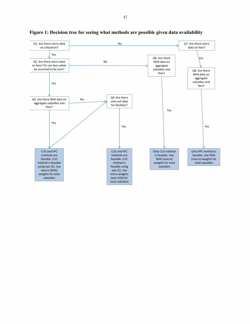
47
Figure 1: Decision tree for seeing what methods are possible given data availability
Q1. Are there micro data on utilization?
Q2. Are there micro data on fees? Or can fees safely
be assumed to be zero?
Yes
Q3. Are there NHA data on aggregate subsidies and
fees?
CUS and FPC methods are feasible. CUC
method is feasible using eqn (3). Use
macro (NHA) weights for total
subsidies
Yes
Q7. Are there micro data on fees?
NoYes
Only FPC method is feasible. Use NHA
(macro) weights for total subsidies
Q4. Are there unit cost data for facilities?
Yes
CUS and FPC methods are feasible. CUC
method is feasible using eqn (2). Use
micro weights (eqn (10)) for total subsidies
Q6. Are there NHA data on
aggregate subsidies and
fees?
Only CUS method is feasible. Use NHA (macro)
weights for total subsidies
No
Yes
No
Yes
Q8. Are there NHA data on
aggregate subsidies and
fees?
Yes

48
Figure 2: Feasibility of different BIA approaches for overall GHE by country

49
Figure 3: Mean GHE CI estimates by subsector and method
-.1 0 .1 .2 .3Concentration Index for GHE
FPC
CUS
CUC NHA
CUC Mic
Note: Sample includes 26 countries with CIs for all 6 subsectors for all 4 methods
IP gov hosp IP priv hosp OP gov hosp OP priv hosp OP govt clinic OP priv clinic Mean
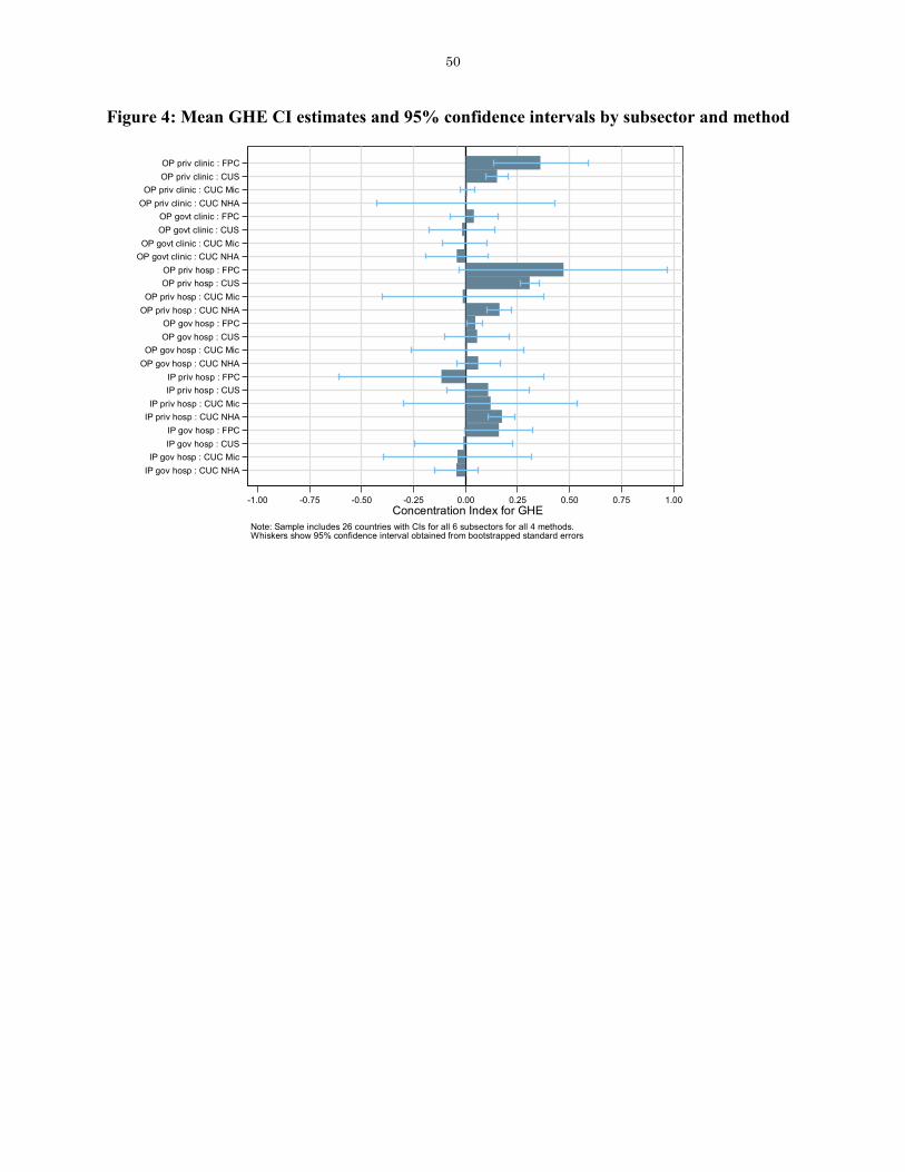
50
Figure 4: Mean GHE CI estimates and 95% confidence intervals by subsector and method
IP gov hosp : CUC NHAIP gov hosp : CUC Mic
IP gov hosp : CUSIP gov hosp : FPC
IP priv hosp : CUC NHAIP priv hosp : CUC Mic
IP priv hosp : CUSIP priv hosp : FPC
OP gov hosp : CUC NHAOP gov hosp : CUC Mic
OP gov hosp : CUSOP gov hosp : FPC
OP priv hosp : CUC NHAOP priv hosp : CUC Mic
OP priv hosp : CUSOP priv hosp : FPC
OP govt clinic : CUC NHAOP govt clinic : CUC Mic
OP govt clinic : CUSOP govt clinic : FPC
OP priv clinic : CUC NHAOP priv clinic : CUC Mic
OP priv clinic : CUSOP priv clinic : FPC
-1.00 -0.75 -0.50 -0.25 0.00 0.25 0.50 0.75 1.00Concentration Index for GHE
Note: Sample includes 26 countries with CIs for all 6 subsectors for all 4 methods.Whiskers show 95% confidence interval obtained from bootstrapped standard errors

51
Figure 5: Sensitivity analysis to see how results are affected by observing outpatient visits only for non-inpatient users
Mexico : IP
Mexico : OP
Mexico : PRIVMexico : PUBLMexico : TOTAL
Mexico : ipadm_ghospMexico : ipadm_phosp
Mexico : opvis_gclin
Mexico : opvis_ghospMexico : opvis_pclinMexico : opvis_phosp
Philippines : ipadm_ghosp
Philippines : ipadm_phosp
Philippines : opvis_gclin
Philippines : opvis_ghosp
Philippines : opvis_pclin
Philippines : opvis_phosp
Slovenia : IP
Slovenia : OP
Slovenia : PRIVSlovenia : PUBLSlovenia : TOTAL
Slovenia : ipadm_ghosp
Slovenia : ipadm_phosp
Slovenia : opvis_gclin
Slovenia : opvis_ghosp
Slovenia : opvis_pclinSlovenia : opvis_phosp
-0.1
0.0
0.1
0.2
0.3
0.4
Con
c. In
dex
for G
HE
: Orig
inal
-0.1 0.0 0.1 0.2 0.3 0.4
Conc. Index for GHE: AlternativeCorrelation = 0.997
CUS NHA
Mexico : IP
Mexico : OP
Mexico : PRIV
Mexico : PUBLMexico : TOTAL
Mexico : ipadm_ghospMexico : ipadm_phosp
Mexico : opvis_gclin
Mexico : opvis_ghospMexico : opvis_pclinMexico : opvis_phosp
Philippines : IP
Philippines : OP
Philippines : PRIV
Philippines : PUBL
Philippines : TOTAL
Philippines : ipadm_ghosp
Philippines : ipadm_phosp
Philippines : opvis_gclin
Philippines : opvis_ghosp
Philippines : opvis_pclin
Philippines : opvis_phosp
Slovenia : IP
Slovenia : OP
Slovenia : PRIV
Slovenia : PUBLSlovenia : TOTAL
Slovenia : ipadm_ghosp
Slovenia : ipadm_phosp
Slovenia : opvis_gclin
Slovenia : opvis_ghosp
Slovenia : opvis_pclinSlovenia : opvis_phosp
-0.1
0.0
0.1
0.2
0.3
0.4
Con
c. In
dex
for G
HE
: Orig
inal
-0.1 0.0 0.1 0.2 0.3 0.4
Conc. Index for GHE: AlternativeCorrelation = 0.995
CUS Micro
Mexico : IPMexico : OP
Mexico : PRIV
Mexico : PUBLMexico : TOTALMexico : ipadm_ghosp
Mexico : ipadm_phosp
Mexico : opvis_gclin
Mexico : opvis_ghospMexico : opvis_pclinMexico : opvis_phosp
Slovenia : IP
Slovenia : OP
Slovenia : PRIV
Slovenia : PUBLSlovenia : TOTAL
Slovenia : ipadm_ghosp
Slovenia : ipadm_phosp
Slovenia : opvis_gclin
Slovenia : opvis_ghosp
Slovenia : opvis_pclinSlovenia : opvis_phosp
-0.1
0.0
0.1
0.2
0.3
Con
c. In
dex
for G
HE
: Orig
inal
-0.1 0.0 0.1 0.2 0.3
Conc. Index for GHE: AlternativeCorrelation = 0.996
CUC NHA
Mexico : IP
Mexico : OP
Mexico : PRIV
Mexico : PUBLMexico : TOTAL
Mexico : ipadm_ghosp
Mexico : ipadm_phosp
Mexico : opvis_gclin
Mexico : opvis_ghospMexico : opvis_pclinMexico : opvis_phosp
Philippines : IP
Philippines : OP
Philippines : PRIV
Philippines : PUBL
Philippines : TOTAL
Philippines : ipadm_ghosp
Philippines : ipadm_phosp
Philippines : opvis_gclin
Philippines : opvis_ghosp
Philippines : opvis_pclin
Philippines : opvis_phosp
Slovenia : IP
Slovenia : OP
Slovenia : PRIV
Slovenia : PUBLSlovenia : TOTAL
Slovenia : ipadm_ghosp
Slovenia : ipadm_phosp
Slovenia : opvis_gclin
Slovenia : opvis_ghosp
Slovenia : opvis_pclinSlovenia : opvis_phosp
-0.1
0.0
0.1
0.2
0.3
0.4
Con
c. In
dex
for G
HE
: Orig
inal
-0.1 0.0 0.1 0.2 0.3
Conc. Index for GHE: AlternativeCorrelation = 0.908
CUC Micro
Mexico : IP
Mexico : OPMexico : PRIV
Mexico : PUBLMexico : TOTALMexico : ipadm_ghosp
Mexico : ipadm_phospMexico : opvis_gclinMexico : opvis_ghospMexico : opvis_pclinMexico : opvis_phosp
Philippines : ipadm_ghosp
Philippines : ipadm_phosp
Philippines : opvis_gclin
Philippines : opvis_ghosp
Philippines : opvis_pclin
Philippines : opvis_phosp
Slovenia : IP
Slovenia : OP
Slovenia : PRIV
Slovenia : PUBLSlovenia : TOTAL
Slovenia : ipadm_ghosp
Slovenia : ipadm_phosp
Slovenia : opvis_gclin
Slovenia : opvis_ghosp
Slovenia : opvis_pclinSlovenia : opvis_phosp
-1.0
-0.5
0.0
0.5
1.0
Con
c. In
dex
for G
HE
: Orig
inal
-1.0 -0.5 0.0 0.5 1.0
Conc. Index for GHE: AlternativeCorrelation = 1.000
FPC NHA
Mexico : IP
Mexico : OPMexico : PRIVMexico : PUBLMexico : TOTAL
Mexico : ipadm_ghosp
Mexico : ipadm_phospMexico : opvis_gclinMexico : opvis_ghospMexico : opvis_pclinMexico : opvis_phosp
Philippines : IPPhilippines : OP
Philippines : PRIV
Philippines : PUBL
Philippines : TOTAL
Philippines : ipadm_ghosp
Philippines : ipadm_phosp
Philippines : opvis_gclin
Philippines : opvis_ghosp
Philippines : opvis_pclin
Philippines : opvis_phosp
Slovenia : IP
Slovenia : OP
Slovenia : PRIV
Slovenia : PUBLSlovenia : TOTAL
Slovenia : ipadm_ghosp
Slovenia : ipadm_phosp
Slovenia : opvis_gclin
Slovenia : opvis_ghosp
Slovenia : opvis_pclinSlovenia : opvis_phosp
-1.0
-0.5
0.0
0.5
1.0
Con
c. In
dex
for G
HE
: Orig
inal
-1.0 -0.5 0.0 0.5 1.0
Conc. Index for GHE: AlternativeCorrelation = 0.993
FPC Micro
Note: In 'original' results, all WHS data are used. In 'alternative' results, WHS outpatient data are used only when inpatient admission did not occur, per original WHS design

52
Figure 6: Mean GHE CI estimates by subsector
IP gov hosp
IP priv hosp
OP gov hosp
OP priv hosp
OP govt clinic
OP priv clinic
-0.100 -0.075 -0.050 -0.025 0.000 0.025 0.050 0.075 0.100 0.125 0.150 0.175 0.200Concentration Index for GHE
Note: CUS method. Sample includes 69 countries with CIs for all 6 subsectorsWhiskers show 95% confidence interval obtained from bootstrapped standard errors

53
Figure 7: NHA vs. micro shares, by subsector
Bangladesh
Burkina Faso
China
Congo, Rep.
Cote d'IvoireEcuador
EstoniaGeorgia
Ghana
Kazakhstan
Kenya
Lao PDR
MalawiMalaysia
Mali
Mexico
Morocco
Myanmar
Namibia
Pakistan
Slovak Republic
Slovenia
South Africa
Spain
Sri Lanka Ukraine
Uruguay
Vietnam
Zambia
0.0
0.1
0.2
0.3
0.4
0.5
0.6
0.7
0.8
0.9
1.0
NH
A e
stim
ate
0.0 0.1 0.2 0.3 0.4 0.5 0.6 0.7 0.8 0.9 1.0
Micro estimateCorrelation = 0.319
IP gov hosp
Bangladesh
Burkina Faso
China
Congo, Rep.Cote d'Ivoire
Ecuador
Estonia
GeorgiaGhana
Kazakhstan
Kenya
Lao PDR
Malawi
Malaysia
MaliMexico
Morocco
Myanmar
NamibiaPakistan
Slovak RepublicSlovenia
South Africa
Spain Sri LankaUkraine
Uruguay
Vietnam
Zambia
0.0
0.1
0.2
0.3
0.4
0.5
0.6
0.7
0.8
0.9
1.0
NH
A e
stim
ate
0.0 0.1 0.2 0.3 0.4 0.5 0.6 0.7 0.8 0.9 1.0
Micro estimateCorrelation = 0.511
OP gov hosp
Bangladesh
Burkina Faso
China
Congo, Rep.
Cote d'Ivoire
Ecuador
Estonia
GeorgiaGhana
Kazakhstan
Kenya
Lao PDR
Malawi
Malaysia
Mali
Mexico
Morocco
Myanmar
Namibia
Pakistan
Slovak Republic
Slovenia
South Africa
Spain
Sri LankaUkraine
UruguayVietnam
Zambia
0.0
0.1
0.2
0.3
0.4
0.5
0.6
0.7
0.8
0.9
1.0
NH
A e
stim
ate
0.0 0.1 0.2 0.3 0.4 0.5 0.6 0.7 0.8 0.9 1.0
Micro estimateCorrelation = 0.522
OP govt clinic
BangladeshBurkina FasoChinaCongo, Rep.Cote d'IvoireEcuadorEstoniaGeorgiaGhanaKazakhstanKenya
Lao PDR
Malawi
MalaysiaMaliMexicoMoroccoMyanmarNamibiaPakistanSlovak RepublicSlovenia South Africa
Spain
Sri LankaUkraine
Uruguay
VietnamZambia0.0
0.1
0.2
0.3
0.4
0.5
0.6
0.7
0.8
0.9
1.0
NH
A e
stim
ate
0.0 0.1 0.2 0.3 0.4 0.5 0.6 0.7 0.8 0.9 1.0
Micro estimateCorrelation = 0.162
IP priv hosp
BangladeshBurkina FasoChinaCongo, Rep.Cote d'IvoireEcuadorEstoniaGeorgiaGhanaKazakhstan
Kenya
Lao PDR MalawiMalaysiaMaliMexicoMoroccoMyanmarNamibiaPakistanSlovak RepublicSlovenia South AfricaSpain
Sri LankaUkraine
Uruguay
Vietnam Zambia0.0
0.1
0.2
0.3
0.4
0.5
0.6
0.7
0.8
0.9
1.0
NH
A e
stim
ate
0.0 0.1 0.2 0.3 0.4 0.5 0.6 0.7 0.8 0.9 1.0
Micro estimateCorrelation = 0.511
OP priv hosp
BangladeshBurkina FasoChinaCongo, Rep.Cote d'IvoireEcuador
Estonia
GeorgiaGhana
Kazakhstan
KenyaLao PDRMalawiMalaysiaMaliMexicoMoroccoMyanmarNamibiaPakistan
Slovak Republic
SloveniaSouth Africa
Spain
Sri LankaUkraineUruguay
Vietnam
Zambia
0.0
0.1
0.2
0.3
0.4
0.5
0.6
0.7
0.8
0.9
1.0
NH
A e
stim
ate
0.0 0.1 0.2 0.3 0.4 0.5 0.6 0.7 0.8 0.9 1.0
Micro estimateCorrelation = 0.736
OP priv clinic

54
Figure 8: NHA vs. micro CIs, by subsector
Bangladesh
Burkina Faso
China
Congo, Rep.
Cote d'Ivoire
Ecuador
EstoniaEthiopia
Georgia
Ghana
Kazakhstan
KenyaLao PDR
Latvia
Malawi
Malaysia Mali
Mexico
Morocco
Myanmar
Namibia
Nepal
Pakistan
Senegal
Slovak Republic
Slovenia
South Africa
Spain
Sri Lanka
Ukraine
Uruguay
Vietnam
Zambia
-0.2
-0.1
0.0
0.1
0.2
0.3
Con
c. In
dex
for G
HE
: NH
A e
stim
ate
-0.1 0.0 0.1 0.2 0.3
Conc. Index for GHE: Micro estimateCorrelation = 0.813
Inpatient
Bangladesh
Burkina FasoChina
Congo, Rep.
Cote d'Ivoire
Czech Republic
Ecuador
Estonia
Georgia
Ghana
KazakhstanKenya
Lao PDR
Malawi
Malaysia
Mali
Mexico
Morocco
Myanmar
Namibia
Pakistan
Slovak Republic
Slovenia
South Africa
Spain
Sri Lanka
UkraineUruguay
Vietnam
Zambia
-0.1
0.0
0.1
0.2
0.3
Con
c. In
dex
for G
HE
: NH
A e
stim
ate
-0.1 0.0 0.1 0.2 0.3
Conc. Index for GHE: Micro estimateCorrelation = 0.616
Outpatient
Bangladesh
Burkina FasoChina
Congo, Rep.
Cote d'Ivoire
Ecuador
Estonia
Georgia
Ghana
Kazakhstan
Kenya
Lao PDR
LatviaMalawi
Malaysia
MaliMexico Morocco
Myanmar
Namibia
Pakistan
Senegal
Slovak Republic
Slovenia
South Africa
Spain
Sri Lanka
Ukraine
Uruguay
Vietnam
Zambia
-0.4
-0.2
0.0
0.2
0.4
Con
c. In
dex
for G
HE
: NH
A e
stim
ate
-0.3 -0.2 -0.1 0.0 0.1 0.2
Conc. Index for GHE: Micro estimateCorrelation = 0.866
Public
Estonia
KazakhstanKenya
Malawi
Mali
Slovak Republic
South Africa
Spain
UruguayZambia
-0.2
0.0
0.2
0.4
0.6
0.8
Con
c. In
dex
for G
HE
: NH
A e
stim
ate
-0.4 -0.2 0.0 0.2 0.4 0.6
Conc. Index for GHE: Micro estimateCorrelation = 0.985
Private
Bangladesh
Burkina FasoChina
Congo, Rep.
Cote d'Ivoire
Ecuador
Estonia
Georgia
Ghana
Kazakhstan
Kenya
Lao PDR
Malawi
Malaysia
Mali
Mexico Morocco
Myanmar
Namibia
Pakistan
Slovak Republic
Slovenia
South Africa
Spain
Sri Lanka
Ukraine
Uruguay
Vietnam
Zambia
-0.1
0.0
0.1
0.2
0.3
Con
c. In
dex
for G
HE
: NH
A e
stim
ate
-0.1 0.0 0.1 0.2
Conc. Index for GHE: Micro estimateCorrelation = 0.625
Total
Note: CUS method. Sample includes 29 countries with CIs for all 4 subtotals and total, with both NHA- and micro-based estimates

55
Figure 9: Mean GHE CI estimates by subtotal
Inpatient
Outpatient
Public
Private
Total
-0.05 -0.03 0.00 0.03 0.05 0.07 0.10 0.13 0.15Concentration Index for GHE
Note: CUS method. NHA unless unavailable in which case Micro used.Sample includes 66 countries with CIs for all 4 subtotals and total.Whiskers show 95% confidence interval obtained from bootstrapped standard errors

56
Figure 10: Overall GHE CI estimates, by country
South AfricaSri LankaMalaysia
AustriaEcuador
Slovak RepublicGermanyNamibia
FranceDominican Republic
CroatiaKazakhstan
United Arab EmiratesAustraliaZambia
MauritiusBelgiumSlovenia
IsraelCongo, Rep.Netherlands
MaliLatvia
Bosnia and HerzegovinaSwedenMorocco
MexicoEthiopia
BangladeshMalawi
SwazilandDenmark
EstoniaPortugalUkraine
KenyaRussian Federation
NorwayLuxembourg
SenegalZimbabwe
FinlandGreeceTunisia
SpainCzech Republic
GhanaUruguay
NepalPakistan
Cote d'IvoireIndia
HungaryBrazil
Burkina FasoGeorgia
MauritaniaChina
Lao PDRParaguay
PhilippinesChad
GuatemalaVietnam
ComorosMyanmar
-0.30 -0.25 -0.20 -0.15 -0.10 -0.05 0.00 0.05 0.10 0.15 0.20 0.25 0.30 0.35 0.40Concentration Index for GHE
Low Income Lower Middle-Income Upper Middle-Income High Income 95% CI
Note: Total GHE computed using CUS method. Subsector concentration indices weighted by NHA shares where available;micro shares used otherwise. Sample includes 66 countries.Whiskers show 95% confidence interval obtained from bootstrapped standard errors.26 of the concentration indices are significant at the 95% level
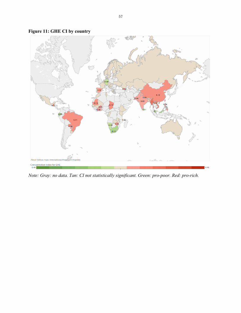
57
Figure 11: GHE CI by country
Note: Gray: no data. Tan: CI not statistically significant. Green: pro-poor. Red: pro-rich.
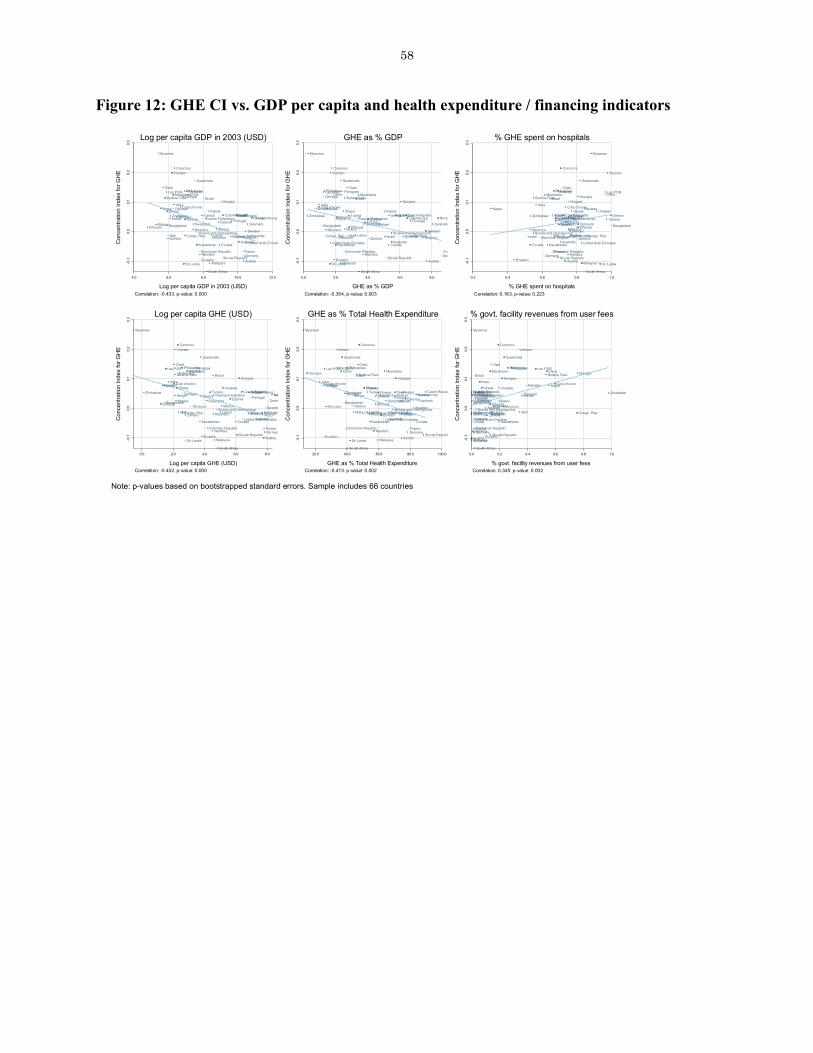
58
Figure 12: GHE CI vs. GDP per capita and health expenditure / financing indicators
Australia
Austria
Bangladesh
BelgiumBosnia and Herzegovina
BrazilBurkina Faso
Chad
China
Comoros
Congo, Rep.
Cote d'Ivoire
Croatia
Czech Republic
Denmark
Dominican Republic
Ecuador
EstoniaEthiopia
Finland
France
Georgia
Germany
GhanaGreece
Guatemala
HungaryIndia
Israel
Kazakhstan
Kenya
Lao PDR
Latvia
Luxembourg
Malawi
Malaysia
Mali
Mauritania
Mauritius
MexicoMorocco
Myanmar
Namibia
Nepal
Netherlands
Norway
Pakistan
ParaguayPhilippines
PortugalRussian FederationSenegal
Slovak Republic
Slovenia
South Africa
Spain
Sri Lanka
Swaziland
Sweden
TunisiaUkraine
United Arab Emirates
Uruguay
Vietnam
Zambia
Zimbabwe
-0.1
0.0
0.1
0.2
0.3
Con
cent
ratio
n In
dex
for G
HE
4.0 6.0 8.0 10.0 12.0
Log per capita GDP in 2003 (USD)Correlation: -0.433. p-value: 0.000
Log per capita GDP in 2003 (USD)
Australia
Austria
Bangladesh
BelgiumBosnia and Herzegovina
BrazilBurkina Faso
Chad
China
Comoros
Congo, Rep.
Cote d'Ivoire
Croatia
Czech Republic
Denmark
Dominican Republic
Ecuador
EstoniaEthiopia
Finland
France
Georgia
Germany
GhanaGreece
Guatemala
HungaryIndia
Israel
Kazakhstan
Kenya
Lao PDR
Latvia
Luxembourg
Malawi
Malaysia
Mali
Mauritania
Mauritius
MexicoMorocco
Myanmar
Namibia
Nepal
Netherlands
Norway
Pakistan
ParaguayPhilippines
PortugalRussian FederationSenegal
Slovak Republic
Slovenia
South Africa
Spain
Sri Lanka
Swaziland
Sweden
TunisiaUkraine
United Arab Emirates
Uruguay
Vietnam
Zambia
Zimbabwe
-0.1
0.0
0.1
0.2
0.3
Con
cent
ratio
n In
dex
for G
HE
0.0 2.0 4.0 6.0 8.0
GHE as % GDPCorrelation: -0.354. p-value: 0.003
GHE as % GDP
Australia
Austria
Bangladesh
BelgiumBosnia and Herzegovina
BrazilBurkina Faso
Chad
China
Comoros
Congo, Rep.
Cote d'Ivoire
Croatia
Czech Republic
Denmark
Dominican Republic
Ecuador
EstoniaEthiopia
Finland
France
Georgia
Germany
GhanaGreece
Guatemala
HungaryIndia
Israel
Kazakhstan
Kenya
Lao PDR
Latvia
Luxembourg
Malawi
Malaysia
Mali
Mauritania
Mauritius
MexicoMorocco
Myanmar
Namibia
Nepal
Netherlands
Norway
Pakistan
ParaguayPhilippines
PortugalRussian FederationSenegal
Slovak Republic
Slovenia
South Africa
Spain
Sri Lanka
Swaziland
Sweden
TunisiaUkraine
United Arab Emirates
Uruguay
Vietnam
Zambia
Zimbabwe
-0.1
0.0
0.1
0.2
0.3
Con
cent
ratio
n In
dex
for G
HE
0.2 0.4 0.6 0.8 1.0
% GHE spent on hospitalsCorrelation: 0.163. p-value: 0.223
% GHE spent on hospitals
Australia
Austria
Bangladesh
BelgiumBosnia and Herzegovina
BrazilBurkina Faso
Chad
China
Comoros
Congo, Rep.
Cote d'Ivoire
Croatia
Czech Republic
Denmark
Dominican Republic
Ecuador
EstoniaEthiopia
Finland
France
Georgia
Germany
GhanaGreece
Guatemala
HungaryIndia
Israel
Kazakhstan
Kenya
Lao PDR
Latvia
Luxembourg
Malawi
Malaysia
Mali
Mauritania
Mauritius
MexicoMorocco
Myanmar
Namibia
Nepal
Netherlands
Norway
Pakistan
ParaguayPhilippines
PortugalRussian FederationSenegal
Slovak Republic
Slovenia
South Africa
Spain
Sri Lanka
Swaziland
Sweden
TunisiaUkraine
United Arab Emirates
Uruguay
Vietnam
Zambia
Zimbabwe
-0.1
0.0
0.1
0.2
0.3
Con
cent
ratio
n In
dex
for G
HE
0.0 2.0 4.0 6.0 8.0
Log per capita GHE (USD)Correlation: -0.452. p-value: 0.000
Log per capita GHE (USD)
Australia
Austria
Bangladesh
BelgiumBosnia and Herzegovina
BrazilBurkina Faso
Chad
China
Comoros
Congo, Rep.
Cote d'Ivoire
Croatia
Czech Republic
Denmark
Dominican Republic
Ecuador
EstoniaEthiopia
Finland
France
Georgia
Germany
GhanaGreece
Guatemala
HungaryIndia
Israel
Kazakhstan
Kenya
Lao PDR
Latvia
Luxembourg
Malawi
Malaysia
Mali
Mauritania
Mauritius
MexicoMorocco
Myanmar
Namibia
Nepal
Netherlands
Norway
Pakistan
ParaguayPhilippines
PortugalRussian FederationSenegal
Slovak Republic
Slovenia
South Africa
Spain
Sri Lanka
Swaziland
Sweden
TunisiaUkraine
United Arab Emirates
Uruguay
Vietnam
Zambia
Zimbabwe
-0.1
0.0
0.1
0.2
0.3
Con
cent
ratio
n In
dex
for G
HE
20.0 40.0 60.0 80.0 100.0
GHE as % Total Health ExpenditureCorrelation: -0.413. p-value: 0.002
GHE as % Total Health Expenditure
Australia
Austria
Bangladesh
BelgiumBosnia and Herzegovina
Brazil Burkina Faso
Chad
China
Comoros
Congo, Rep.
Cote d'Ivoire
Croatia
Czech Republic
Denmark
Dominican Republic
Ecuador
EstoniaEthiopia
Finland
France
Georgia
Germany
GhanaGreece
Guatemala
HungaryIndia
Israel
Kazakhstan
Kenya
Lao PDR
Latvia
Luxembourg
Malawi
Malaysia
Mali
Mauritania
Mauritius
MexicoMorocco
Myanmar
Namibia
Nepal
Netherlands
Norway
Pakistan
ParaguayPhilippines
PortugalRussian Federation Senegal
Slovak Republic
Slovenia
South Africa
Spain
Sri Lanka
Swaziland
Sweden
TunisiaUkraine
United Arab Emirates
Uruguay
Vietnam
Zambia
Zimbabwe
-0.1
0.0
0.1
0.2
0.3
Con
cent
ratio
n In
dex
for G
HE
0.0 0.2 0.4 0.6 0.8 1.0
% govt. facility revenues from user feesCorrelation: 0.345. p-value: 0.002
% govt. facility revenues from user fees
Note: p-values based on bootstrapped standard errors. Sample includes 66 countries

59
Figure 13: GHE CI vs. Indicators of private-sector opt-out
Australia
Austria
Bangladesh
Belgium
Bosnia and Herzegovina
BrazilBurkina Faso
Chad
China
Comoros
Congo, Rep.
Cote d'Ivoire
Croatia
Czech Republic
Denmark
Dominican Republic
Ecuador
Estonia
Ethiopia
Finland
France
Georgia
Germany
Ghana
Greece
Guatemala
HungaryIndia
Israel
Kazakhstan
Kenya
Lao PDR
Latvia
Luxembourg
Malawi
Malaysia
Mali
Mauritania
Mauritius
MexicoMorocco
Myanmar
Namibia
Nepal
Netherlands
Norway
Pakistan
ParaguayPhilippines
PortugalRussian Federation Senegal
Slovak Republic
Slovenia
South Africa
Spain
Sri Lanka
Swaziland
Sweden
TunisiaUkraine
United Arab Emirates
Uruguay
Vietnam
Zambia
Zimbabwe
-0.1
0.0
0.1
0.2
0.3
CI G
HE
-0.2 0.0 0.2 0.4 0.6
CI private utilizationCorrelation: 0.289. p-value: 0.018. N: 66
CI GHE vs. CI private utilization
Austria
Bangladesh
Bosnia and Herzegovina
BrazilBurkina Faso
Chad
China
Comoros
Congo, Rep.
Cote d'Ivoire
Croatia
Czech Republic
Denmark
Dominican Republic
Ecuador
Estonia
Ethiopia
Finland
France
Georgia
Germany
Ghana
Greece
Guatemala
HungaryIndia
Kazakhstan
Kenya
Lao PDR
Latvia
Luxembourg
Malawi
Malaysia
Mali
Mauritania
Mauritius
MexicoMorocco
Myanmar
Namibia
Nepal
Netherlands
Norway
Pakistan
Paraguay Philippines
Russian Federation Senegal
Slovak Republic
Slovenia
South Africa
Spain
Sri Lanka
Swaziland
Sweden
TunisiaUkraine
United Arab Emirates
Uruguay
Vietnam
Zambia
Zimbabwe
-0.1
0.0
0.1
0.2
0.3
CI G
HE
-0.5 0.0 0.5 1.0
CI fees to private sectorCorrelation: 0.173. p-value: 0.178. N: 62
CI GHE vs. CI fees to private sector
Australia
Austria
Bangladesh
Belgium
Bosnia and Herzegovina
BrazilBurkina Faso
Chad
China
Comoros
Congo, Rep.
Cote d'Ivoire
Croatia
Czech Republic
Denmark
Dominican Republic
Ecuador
Estonia
Ethiopia
Finland
France
Georgia
Germany
Ghana
Greece
Guatemala
HungaryIndia
Israel
Kazakhstan
Kenya
Lao PDR
Latvia
Luxembourg
Malawi
Malaysia
Mali
Mauritania
Mauritius
Mexico Morocco
Myanmar
Namibia
Nepal
Netherlands
Norway
Pakistan
ParaguayPhilippines
PortugalRussian FederationSenegal
Slovak Republic
Slovenia
South Africa
Spain
Sri Lanka
Swaziland
Sweden
TunisiaUkraine
United Arab Emirates
Uruguay
Vietnam
Zambia
Zimbabwe
-0.1
0.0
0.1
0.2
0.3
CI G
HE
0.0 0.2 0.4 0.6 0.8
Private share of utilizationCorrelation: -0.054. p-value: 0.669. N: 66
CI GHE vs. Private share of utilization
Australia
Austria
Bangladesh
Belgium
Bosnia and Herzegovina
BrazilBurkina Faso
Chad
China
Comoros
Congo, Rep.
Cote d'Ivoire
Croatia
Czech Republic
Denmark
Dominican Republic
Ecuador
Estonia
Ethiopia
Finland
France
Georgia
Germany
Ghana
Greece
Guatemala
HungaryIndia
Israel
Kazakhstan
Kenya
Lao PDR
Latvia
Luxembourg
Malawi
Malaysia
Mali
Mauritania
Mauritius
Mexico Morocco
Myanmar
Namibia
Nepal
Netherlands
Norway
Pakistan
ParaguayPhilippines
PortugalRussian FederationSenegal
Slovak Republic
Slovenia
South Africa
Spain
Sri Lanka
Swaziland
Sweden
TunisiaUkraine
United Arab Emirates
Uruguay
Vietnam
Zambia
Zimbabwe
-0.1
0.0
0.1
0.2
0.3
CI G
HE
0.0 0.2 0.4 0.6 0.8 1.0
Private share of feesCorrelation: -0.093. p-value: 0.517. N: 51
CI GHE vs. Private share of fees

60
Figure 14: GHE CI vs. governance indicators
Australia
Austria
Bangladesh
BelgiumBosnia and Herzegovina
BrazilBurkina Faso
Chad
China
Comoros
Congo, Rep.
Cote d'Ivoire
Croatia
Czech Republic
Denmark
Dominican Republic
Ecuador
EstoniaEthiopia
Finland
France
Georgia
Germany
GhanaGreece
Guatemala
HungaryIndia
Israel
Kazakhstan
Kenya
Lao PDR
Latvia
Luxembourg
Malawi
Malaysia
Mali
Mauritania
Mauritius
MexicoMorocco
Myanmar
Namibia
Nepal
Netherlands
Norway
Pakistan
Paraguay Philippines
PortugalRussian FederationSenegal
Slovak Republic
Slovenia
South Africa
Spain
Sri Lanka
Swaziland
Sweden
TunisiaUkraine
United Arab Emirates
Uruguay
Vietnam
Zambia
Zimbabwe
-0.1
0.0
0.1
0.2
0.3
Con
cent
ratio
n In
dex
for G
HE
-2.0 -1.0 0.0 1.0 2.0
VoiceCorrelation: -0.413. p-value: 0.001
Voice
Australia
Austria
Bangladesh
BelgiumBosnia and Herzegovina
BrazilBurkina Faso
Chad
China
Comoros
Congo, Rep.
Cote d'Ivoire
Croatia
Czech Republic
Denmark
Dominican Republic
Ecuador
EstoniaEthiopia
Finland
France
Georgia
Germany
GhanaGreece
Guatemala
HungaryIndia
Israel
Kazakhstan
Kenya
Lao PDR
Latvia
Luxembourg
Malawi
Malaysia
Mali
Mauritania
Mauritius
MexicoMorocco
Myanmar
Namibia
Nepal
Netherlands
Norway
Pakistan
ParaguayPhilippines
PortugalRussian FederationSenegal
Slovak Republic
Slovenia
South Africa
Spain
Sri Lanka
Swaziland
Sweden
TunisiaUkraine
United Arab Emirates
Uruguay
Vietnam
Zambia
Zimbabwe
-0.1
0.0
0.1
0.2
0.3
Con
cent
ratio
n In
dex
for G
HE
-2.0 -1.0 0.0 1.0 2.0
Political StabilityCorrelation: -0.327. p-value: 0.005
Political Stability
Australia
Austria
Bangladesh
BelgiumBosnia and Herzegovina
BrazilBurkina Faso
Chad
China
Comoros
Congo, Rep.
Cote d'Ivoire
Croatia
Czech Republic
Denmark
Dominican Republic
Ecuador
EstoniaEthiopia
Finland
France
Georgia
Germany
GhanaGreece
Guatemala
HungaryIndia
Israel
Kazakhstan
Kenya
Lao PDR
Latvia
Luxembourg
Malawi
Malaysia
Mali
Mauritania
Mauritius
MexicoMorocco
Myanmar
Namibia
Nepal
Netherlands
Norway
Pakistan
Paraguay Philippines
PortugalRussian FederationSenegal
Slovak Republic
Slovenia
South Africa
Spain
Sri Lanka
Swaziland
Sweden
TunisiaUkraine
United Arab Emirates
Uruguay
Vietnam
Zambia
Zimbabwe
-0.1
0.0
0.1
0.2
0.3
Con
cent
ratio
n In
dex
for G
HE
-1.0 0.0 1.0 2.0
Govt. EffectivenessCorrelation: -0.372. p-value: 0.002
Govt. Effectiveness
Australia
Austria
Bangladesh
BelgiumBosnia and Herzegovina
BrazilBurkina Faso
Chad
China
Comoros
Congo, Rep.
Cote d'Ivoire
Croatia
Czech Republic
Denmark
Dominican Republic
Ecuador
EstoniaEthiopia
Finland
France
Georgia
Germany
GhanaGreece
Guatemala
HungaryIndia
Israel
Kazakhstan
Kenya
Lao PDR
Latvia
Luxembourg
Malawi
Malaysia
Mali
Mauritania
Mauritius
MexicoMorocco
Myanmar
Namibia
Nepal
Netherlands
Norway
Pakistan
Paraguay Philippines
PortugalRussian FederationSenegal
Slovak Republic
Slovenia
South Africa
Spain
Sri Lanka
Swaziland
Sweden
TunisiaUkraine
United Arab Emirates
Uruguay
Vietnam
Zambia
Zimbabwe
-0.1
0.0
0.1
0.2
0.3
Con
cent
ratio
n In
dex
for G
HE
-2.0 -1.0 0.0 1.0 2.0
Regulatory QualityCorrelation: -0.433. p-value: 0.000
Regulatory Quality
Australia
Austria
Bangladesh
BelgiumBosnia and Herzegovina
BrazilBurkina Faso
Chad
China
Comoros
Congo, Rep.
Cote d'Ivoire
Croatia
Czech Republic
Denmark
Dominican Republic
Ecuador
EstoniaEthiopia
Finland
France
Georgia
Germany
GhanaGreece
Guatemala
HungaryIndia
Israel
Kazakhstan
Kenya
Lao PDR
Latvia
Luxembourg
Malawi
Malaysia
Mali
Mauritania
Mauritius
Mexico Morocco
Myanmar
Namibia
Nepal
Netherlands
Norway
Pakistan
Paraguay Philippines
PortugalRussian Federation Senegal
Slovak Republic
Slovenia
South Africa
Spain
Sri Lanka
Swaziland
Sweden
TunisiaUkraine
United Arab Emirates
Uruguay
Vietnam
Zambia
Zimbabwe
-0.1
0.0
0.1
0.2
0.3
Con
cent
ratio
n In
dex
for G
HE
-2.0 -1.0 0.0 1.0 2.0
Rule of LawCorrelation: -0.414. p-value: 0.000
Rule of Law
Australia
Austria
Bangladesh
BelgiumBosnia and Herzegovina
BrazilBurkina Faso
Chad
China
Comoros
Congo, Rep.
Cote d'Ivoire
Croatia
Czech Republic
Denmark
Dominican Republic
Ecuador
EstoniaEthiopia
Finland
France
Georgia
Germany
GhanaGreece
Guatemala
HungaryIndia
Israel
Kazakhstan
Kenya
Lao PDR
Latvia
Luxembourg
Malawi
Malaysia
Mali
Mauritania
Mauritius
MexicoMorocco
Myanmar
Namibia
Nepal
Netherlands
Norway
Pakistan
Paraguay Philippines
PortugalRussian FederationSenegal
Slovak Republic
Slovenia
South Africa
Spain
Sri Lanka
Swaziland
Sweden
TunisiaUkraine
United Arab Emirates
Uruguay
Vietnam
Zambia
Zimbabwe
-0.1
0.0
0.1
0.2
0.3
Con
cent
ratio
n In
dex
for G
HE
-1.0 0.0 1.0 2.0 3.0
Control of CorruptionCorrelation: -0.349. p-value: 0.002
Control of Corruption
Note: p-values based on bootstrapped standard errors. Sample includes 66 countries

61
References
Acemoglu, D., A. Finkelstein and M. J. Notowidigdo (2012). "Income and Health Spending: Evidence from Oil Price Shocks." Review of Economics and Statistics 95(4): 1079-1095.
Adam, T., D. B. Evans and C. J. Murray (2003). "Econometric estimation of country-specific hospital costs." Cost Eff Resour Alloc 1(1): 3.
Besley, T. and S. Coate (1991). "Public Provision of Private Goods and the Redistribution of Income." American Economic Review 81(4): 979-984.
Burger, R., C. Bredenkamp, C. Grobler and S. van der Berg (2012). "Have Public Health Spending and Access in South Africa Become More Equitable since the End of Apartheid?" Development Southern Africa 29 5: 681-703.
Castro-Leal, F., J. Dayton, L. Demery and K. Mehra (1999). "Public social spending in Africa: Do the poor benefit?" World Bank Research Observer 14(1): 49-72.
Castro-Leal, F., J. Dayton, L. Demery and K. Mehra (2000). "Public spending on health care in Africa: do the poor benefit?" Bulletin of the World Health Organization 78(1): 66-74.
Chaudhury, N., J. Hammer, M. Kremer, K. Muralidharan and F. H. Rogers (2006). "Missing in Action: Teacher and Health Worker Absence in Developing Countries." Journal of Economic Perspectives 20 1: 91-116.
Chen, Z. and K. Roy (2009). "Calculating Concentration Index with Repetitive Values of Indicators of Economic Welfare." Journal of Health Economics 28 1: 169-175.
Costa-Font, J., M. Gemmill and G. Rubert (2011). "Biases in the healthcare luxury good hypothesis?: a meta-regression analysis." Journal of the Royal Statistical Society: Series A (Statistics in Society) 174(1): 95-107.
Davoodi, H. R., E. R. Tiongson and S. S. Asawanuchit (2010). "Benefit Incidence of Public Education and Health Spending Worldwide: Evidence from a New Database." Poverty and Public Policy 2 2.
Devarajan, S. and R. Reinikka (2004). "Making Services Work for Poor People." Journal of African Economies 13(suppl 1): i142-i166.
Filmer, D. (2003). The Incidence of Public Expenditures on Health and Education. Washington,D.C., World Bank.
Gerdtham, U.-G. and B. Jönsson (2000). International comparisons of health expenditure: theory, data and econometric analysis. Handbook of Health Economics. A. J. Culyer and J. Newhouse. Amsterdam, Elsevier. 1: 11-53.
Gertler, P., L. Locay and W. Sanderson (1987). "Are user fees regressive?: The welfare implications of health care financing proposals in Peru." Journal of Econometrics 36(1–2): 67-88.
Good, I. J. (1992). "The Bayes/Non-Bayes Compromise: A Brief Review." Journal of the American Statistical Association 87(419): 597-606.
Heijink, R., K. Xu, P. Saksena and D. Evans (2011). Validity and comparability of out-of-pocket health expenditure from household surveys: a review of the literature and current survey instruments. Geneva, WHO.
Kakwani, N., A. Wagstaff and E. van Doorslaer (1997). "Socioeconomic Inequalities in Health: Measurement, Computation, and Statistical Inference." Journal of Econometrics 77 1: 87-103.
Kaufmann, D. and A. Kraay (2002). "Growth without Governance." Economia: Journal of the Latin American and Caribbean Economic Association 3 1: 169-215.
Kaufmann, D., A. Kraay and M. Mastruzzi (2009). Governance matters VIII: aggregate and individual governance indicators 1996-2008. The World Bank, Policy Research Working Paper Series, 4978.
Kaufmann, D., A. Kraay and P. Zoido-Lobatón (1999). Governance Matters. Washington DC, World Bank.
Lanjouw, P. and M. Ravallion (1999). "Benefit incidence, public spending reforms, and the timing of program capture." World Bank Economic Review 13: 257-273.

62
Lindelow, M. (2008). Tracking Public Money in the Health Sector in Mozambique: Conceptual and Practical Challenges. Are You Being Served? New Tools for Measuring Service Delivery. S. Amin, J. Das and M. Goldstein. Washington, D.C., World Bank: 173-189.
Lu, C., B. Chin, G. Li and C. J. Murray (2009). "Limitations of methods for measuring out-of-pocket and catastrophic private health expenditures." Bull World Health Organ 87(3): 238-244, 244A-244D.
Mahal, A., J. Singh, F. Afridi and V. Lamba (2001). Who Benefits From Public Health Spending in India. Washington DC, World Bank.
McPake, B., D. Asiimwe, F. Mwesigye, M. Ofumbi, L. Ortenblad, et al. (1999). "Informal economic activities of public health workers in Uganda: implications for quality and accessibility of care." Social Science & Medicine 49(7): 849-865.
Musgrove, P., R. Zeramdini and G. Carrin (2002). "Basic patterns in national health expenditure." Bull World Health Organ 80(2): 134-142.
O'Donnell, O., E. van Doorslaer, R. P. Rannan-Eliya, A. Somanathan, S. R. Adhikari, et al. (2007). "The incidence of public spending on healthcare: Comparative evidence from Asia." World Bank Economic Review 21 1: 93-123.
Raban, M. Z., R. Dandona and L. Dandona (2013). "Variations in catastrophic health expenditure estimates from household surveys in India." Bull World Health Organ 91(10): 726-735.
Wagstaff, A. (2012). "Benefit-incidence analysis: are government health expenditures more pro-rich than we think?" Health Economics 21(4): 351-366.
World Bank (2003). World Development Report 2004: Making Service Work for Poor People. Oxford, Oxford University Press and the World Bank.
Younger, S. D. (2003). "Benefits on the margin: Observations on marginal benefit incidence." World Bank Economic Review 17(1): 89-106.

63
Appendix
Table A1: Data availability and implied feasibility of BIA based on decision tree, by country and method Country
WHS Sample
Size
WHS includes
utilization
WHS includes
fees
NHA case
unit cost available
CUC is feasible
CUS is feasible
FPC is feasible
Australia 1,745 Y N B Y N Y N Austria 1,055 Y N B Y N Y N Bangladesh 5,929 Y Y B Y Y Y Y Belgium 478 Y N B Y N Y N Bosnia and Herzegovina 802 Y Y F Y Y Y Y Brazil 4,900 Y Y F Y Y Y Y Burkina Faso 4,912 Y Y D Y Y Y Y Chad 4,438 Y Y F Y Y Y Y China 3,991 Y Y B Y Y Y Y Comoros 1,817 Y Y F Y Y Y Y Congo, Rep. 2,706 Y Y B Y Y Y Y Cote d'Ivoire 3,111 Y Y A Y Y Y Y Croatia 978 Y Y F Y Y Y Y Czech Republic 712 Y Y B Y Y Y Y Denmark 1,002 Y N B Y N Y N Dominican Republic 4,903 Y Y F Y Y Y Y Ecuador 4,406 Y Y E Y Y Y Y Estonia 1,015 Y Y B Y Y Y Y Ethiopia 4,294 Y Y A Y Y Y Y Finland 1,013 Y N A Y N Y N France 1,007 Y N B Y N Y N Georgia 2,751 Y Y B Y Y Y Y Germany 1,257 Y N B Y N Y N Ghana 4,095 Y Y B Y Y Y Y Greece 999 Y N B Y N Y N Guatemala 4,699 Y Y F Y Y Y Y Hungary 134 Y Y B Y Y Y Y India 10,208 Y Y F Y Y Y Y Ireland 1,014 Y N F Y N N N Israel 720 Y N B Y N Y N Italy 1,000 Y N F Y N N N Kazakhstan 4,497 Y Y B Y Y Y Y Kenya 4,584 Y Y A Y Y Y Y Lao PDR 4,972 Y Y E Y Y Y Y Latvia 832 Y Y B Y Y Y Y Luxembourg 700 Y N B Y N Y N Malawi 5,481 Y Y A Y Y Y Y Malaysia 6,011 Y Y A Y Y Y Y Mali 3,953 Y* Y A Y Y Y Y Mauritania 3,679 Y Y F Y Y Y Y Mauritius 3,957 Y Y F Y Y Y Y Mexico 38,515 Y Y E Y Y Y Y Morocco 4,696 Y Y B Y Y Y Y Myanmar 6,045 Y Y E Y Y Y Y Namibia 4,233 Y Y B Y Y Y Y Nepal 8,781 Y Y A Y Y Y Y Netherlands 1,091 Y N C Y N Y N Norway 826 Y N B Y N Y N Pakistan 6,456 Y Y D Y Y Y Y Paraguay 5,273 Y Y F Y Y Y Y Philippines 10,068 Y Y F Y Y Y Y Portugal 1,029 Y N A Y N Y N Russian Federation 4,422 Y Y F Y Y Y Y

64
Country WHS
Sample Size
WHS includes
utilization
WHS includes
fees NHA case
unit cost available
CUC is feasible
CUS is feasible
FPC is feasible
Senegal 3,107 Y Y A Y Y Y Y Slovak Republic 1,737 Y Y B Y Y Y Y Slovenia 666 Y Y B Y Y Y Y South Africa 2,351 Y Y D Y Y Y Y Spain 5,580 Y Y A Y Y Y Y Sri Lanka 6,733 Y Y B Y Y Y Y Swaziland 2,783 Y Y F Y Y Y Y Sweden 999 Y N B Y N Y N Tunisia 5,114 Y Y F Y Y Y Y Turkey 1,167 N N N N N Ukraine 1,199 Y Y B Y Y Y Y United Arab Emirates 2,596 Y Y F Y Y Y Y United Kingdom 2,967 Y N F Y N N N Uruguay 4,171 Y Y A Y Y Y Y Vietnam 4,135 Y Y B Y Y Y Y Zambia 4,106 Y Y A Y Y Y Y Zimbabwe 1,745 Y Y F Y Y Y Y No. countries Y or A-E 69 52 49 69 52 66 52 Notes: N indicates No, Y Yes. For ‘NHA case’ code, see Table 2 in the text. * Feasibility for each method is computed using the decision tree in Figure 1 in the text.

65
Table A2: NHA and other information used to construct GHE by subsector Country Title of HNA Other documents used Year Case
Australia Health Expenditure Australia, 2007-08 2006/2007 B
Austria OECD NHA tables 2004 B
Bangladesh SHA-Based Health Accounts in the Asia/Pacific Region, Bangladesh, 2006
2004/2005 B
Belgium OECD NHA tables
Health Systems in Transition, Belgium, 2010
2003 B
Bosnia and Herzegovina N/A F
Brazil N/A F
Burkina Faso Construction des Comptes Nationaux de la Santé pour 2003
2003 D
Chad N/A F
China SHA-Based Health Accounts in the Asia/Pacific Region, China, 1990-2006
2005 B
Comoros N/A F
Congo, Rep. Comptes Nationaux de la Santé 2008-2009 2008 B
Cote d'Ivoire Comptes Nationaux de la Santé, exercices 2007, 2008 2007 A
Croatia N/A F Czech Republic OECD NHA tables
Health Systems in Transition, Czech Republic, 2005
2003 B
Denmark OECD NHA tables
Health Systems in Transition, Denmark, 2007
2003 B
Dominican Republic N/A F
Ecuador Cuentas Nacionales de Salud: Ecuador, 1998 1998 E
Estonia OECD NHA tables
Health Systems in Transition, Estonia, 2004
2003 B
Ethiopia Ethiopia’s Third National Health Accounts, 2004/05 2004/2005 A
Finland OECD NHA tables 2003 A
France OECD NHA tables
Health Systems in Transition, France, 2004
2004 B
Georgia National Health Accounts For Georgia 2001-2003
Health Systems in Transition, Georgia, 2009
2003 B
Germany OECD NHA tables
Health Systems in Transition, Germany, 2004
2003 B
Ghana National Health Accounts, Ghana 2002 2002 B
Greece OECD NHA tables 2003 B Guatemala N/A F
Hungary OECD NHA tables
Health Systems in Transition, Hungary, 2011
2003 B
India N/A F Ireland N/A F Israel OECD NHA tables 2006 B Italy N/A F Kazakhstan Kazakhstan NHA Report for 2010 B
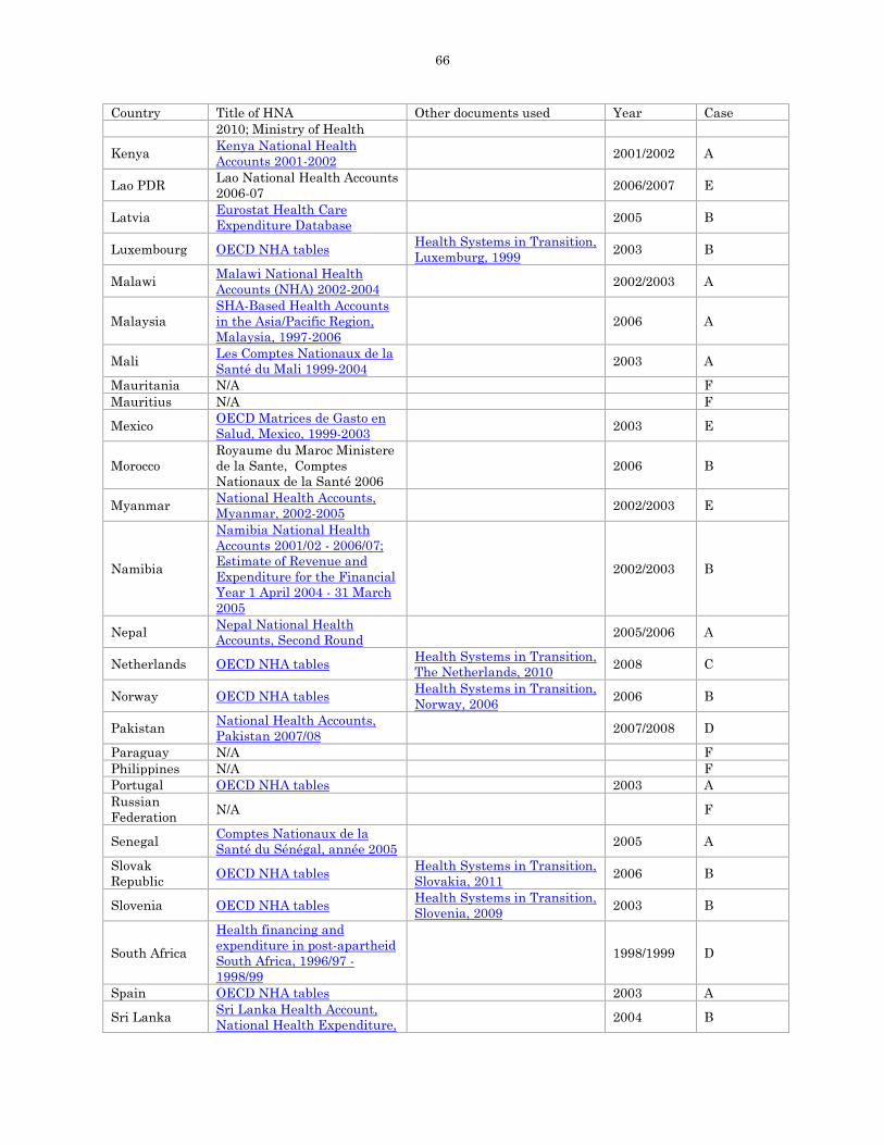
66
Country Title of HNA Other documents used Year Case 2010; Ministry of Health
Kenya Kenya National Health Accounts 2001-2002 2001/2002 A
Lao PDR Lao National Health Accounts 2006-07 2006/2007 E
Latvia Eurostat Health Care Expenditure Database 2005 B
Luxembourg OECD NHA tables
Health Systems in Transition, Luxemburg, 1999
2003 B
Malawi Malawi National Health Accounts (NHA) 2002-2004 2002/2003 A
Malaysia SHA-Based Health Accounts in the Asia/Pacific Region, Malaysia, 1997-2006
2006 A
Mali Les Comptes Nationaux de la Santé du Mali 1999-2004 2003 A
Mauritania N/A F Mauritius N/A F
Mexico OECD Matrices de Gasto en Salud, Mexico, 1999-2003 2003 E
Morocco Royaume du Maroc Ministere de la Sante, Comptes Nationaux de la Santé 2006 2006 B
Myanmar National Health Accounts, Myanmar, 2002-2005 2002/2003 E
Namibia
Namibia National Health Accounts 2001/02 - 2006/07; Estimate of Revenue and Expenditure for the Financial Year 1 April 2004 - 31 March 2005
2002/2003 B
Nepal Nepal National Health Accounts, Second Round 2005/2006 A
Netherlands OECD NHA tables
Health Systems in Transition, The Netherlands, 2010
2008 C
Norway OECD NHA tables
Health Systems in Transition, Norway, 2006
2006 B
Pakistan National Health Accounts, Pakistan 2007/08 2007/2008 D
Paraguay N/A F Philippines N/A F Portugal OECD NHA tables 2003 A Russian Federation N/A F
Senegal Comptes Nationaux de la Santé du Sénégal, année 2005 2005 A
Slovak Republic OECD NHA tables
Health Systems in Transition, Slovakia, 2011
2006 B
Slovenia OECD NHA tables
Health Systems in Transition, Slovenia, 2009
2003 B
South Africa Health financing and expenditure in post-apartheid South Africa, 1996/97 - 1998/99
1998/1999 D
Spain OECD NHA tables 2003 A
Sri Lanka Sri Lanka Health Account, National Health Expenditure, 2004 B

67
Country Title of HNA Other documents used Year Case 1990-2008
Swaziland N/A F
Sweden OECD NHA tables
Health Systems in Transition, Sweden, 2005
2003 B
Tunisia National Health Accounts in Tunisia: Results for Years 2004 and 2005
2004 F
Ukraine Ukraine National Health Accounts 2003-2004, Volume 1
2003 B
United Arab Emirates N/A F
United Kingdom N/A F
Uruguay Cuentas Nacionales de Salud en el Uruguay 2000 2000 A
Vietnam
Ministry of Health National Health Account Implementation in Viet Nam Period From 2000-2006
2006 B
Zambia Zambia National Health Accounts 2002: Main Findings 2002 A
Zimbabwe N/A F Notes: N/A indicates NHA does not appear to be available. Absence of hyperlink indicates document is not available online. For ‘NHA case’ code, see Table 2 in the text.

68
Table A3: Mean GHE CI estimates by subsector and method CI se pval ci95_lo ci95_up cuc_nha ipadm_ghosp -0.044 0.054 0.424 -0.150 0.063 ipadm_phosp 0.174 0.033 0.000 0.110 0.239 opvis_ghosp 0.063 0.053 0.238 -0.041 0.167 opvis_phosp 0.164 0.030 0.000 0.104 0.223 opvis_gclin -0.041 0.076 0.590 -0.190 0.108 opvis_pclin 0.001 0.218 0.995 -0.425 0.428 cuc_mic ipadm_ghosp -0.039 0.182 0.830 -0.396 0.318 ipadm_phosp 0.120 0.213 0.575 -0.298 0.538 opvis_ghosp 0.009 0.138 0.950 -0.262 0.279 opvis_phosp -0.012 0.198 0.951 -0.400 0.376 opvis_gclin -0.005 0.055 0.924 -0.112 0.102 opvis_pclin 0.008 0.017 0.616 -0.024 0.041 cus ipadm_ghosp -0.009 0.120 0.939 -0.244 0.225 ipadm_phosp 0.108 0.102 0.290 -0.091 0.308 opvis_ghosp 0.056 0.080 0.488 -0.101 0.213 opvis_phosp 0.310 0.023 0.000 0.265 0.356 opvis_gclin -0.016 0.081 0.843 -0.175 0.143 opvis_pclin 0.150 0.027 0.000 0.097 0.204 fpc ipadm_ghosp 0.159 0.082 0.057 -0.002 0.321 ipadm_phosp -0.115 0.251 0.649 -0.607 0.378 opvis_ghosp 0.047 0.019 0.016 0.010 0.085 opvis_phosp 0.471 0.255 0.070 -0.030 0.972 opvis_gclin 0.041 0.059 0.488 -0.074 0.156 opvis_pclin 0.362 0.116 0.003 0.134 0.590 Note: Sample includes 26 countries with CIs for all 6 subsectors for all 4 methods

69
Table A4: Mean GHE CI estimates by subsector CI se pval ci95_lo ci95_up ipadm_ghosp 0.003 0.017 0.862 -0.031 0.037 ipadm_phosp 0.110 0.054 0.045 0.003 0.217 opvis_ghosp 0.006 0.024 0.799 -0.041 0.054 opvis_phosp 0.168 0.061 0.006 0.049 0.287 opvis_gclin -0.022 0.018 0.211 -0.057 0.013 opvis_pclin 0.096 0.031 0.002 0.034 0.158 Note: CUS method. Sample includes 69 countries with CIs for all 6 subsectors Table A5: Mean GHE CI estimates by subtotal CI se pval ci95_lo ci95_up IP 0.021 0.016 0.177 -0.009 0.052 OP 0.037 0.015 0.016 0.007 0.067 PUBL 0.006 0.014 0.660 -0.021 0.034 PRIV 0.119 0.038 0.002 0.045 0.193 TOTAL 0.032 0.013 0.012 0.007 0.057 Note: CUS method. Subsector concentration indices weighted by NHA shares where available; micro shares used otherwise. Sample includes 66 countries with CIs for all 4 subtotals and total Table A6: Differences between means of WHS and non-WHS countries on correlates of GHE concentration index
All countries with data on variable Countries with data on all variables N WHS Other t p>t N WHS Other t p>t Log GDP per capita 198 8.064 7.557 0.75 0.457 165 8.093 7.877 2.09 0.038 Log GHE per capita 185 4.660 3.972 1.53 0.127 165 4.660 4.188 2.15 0.033 GHE as % GDP 187 3.826 3.155 0.48 0.634 165 3.879 3.645 2.43 0.016 GHE as % THE 187 55.428 53.909 -0.66 0.513 165 56.071 57.471 0.70 0.485 Voice 174 0.117 -0.263 2.75 0.007 165 0.172 -0.311 2.85 0.005 Political stability 174 -0.011 -0.176 1.31 0.192 165 0.029 -0.214 1.33 0.184 Government effectiveness
174 0.274 -0.218 3.53 0.001 165 0.315 -0.267 3.51 0.001
Regulatory quality 174 0.222 -0.216 3.22 0.002 165 0.289 -0.268 3.44 0.001 Rule of law 174 0.116 -0.251 2.63 0.009 165 0.168 -0.290 2.74 0.007 Control of corruption 174 0.182 -0.194 2.62 0.009 165 0.225 -0.229 2.67 0.008 Note: Data are from WDI and WGI. “Other” means non-WHS countries.