who bears firm-level risk?
TRANSCRIPT

Who Bears Firm-Level Risk?
Implications for Cash Flow Volatility ∗
Mindy Xiaolan Zhang†
February 4, 2014
Abstract
Public firms in the United States that provide better insurance against pro-ductivity shocks to their workers experience higher cash flow volatility. Differencein intra-firm risk sharing between workers and capital owners accounts for morethan 50% of the variation in firm-level cash flow volatility. I develop a theory inwhich wages can act either as a hedge or as leverage, depending on the history ofthe productivity shocks the firm has faced. Heterogeneous roles of workers in thefirm are derived by analyzing the dynamic equilibrium wage contracts betweenrisk-neutral owners and risk-averse workers who can leave with a fraction of theaccumulated human capital. Owners of the firm will optimally bear more riskwhen the current value of the firm’s human capital is lower than the peak valueit has reached. The model successfully explains the joint distribution of cash flowvolatility and the wage-output sensitivity. Also, the model produces predictionsfor the dynamics of cash flow volatility that are consistent with the time seriesproperties of the firm-level data.
Keywords: Dynamic Contracts, Firm-Level Cash Flow Volatility, Wage-Output Sensi-
tivity, Human Capital Investment
∗I am deeply grateful to my advisor Hanno Lustig, as well as to Antonio Bernardo, Andrea Eisfeldt, andMark Garmaise for invaluable support, ideas and advice. For helpful comments and discussions, I would liketo thank Daniel Andrei, Andrew Atkeson, Simon Board, Jonathan Berk, Bruce Carlin, Mikhail Chernov,Mark Grinblatt, Barney Hartman-Glaser, Hugo Hopenhayn, Yaron Levi, Jiasun Li, Robert Novy-Max, IchiroObara, Lukas Schmid, Qi Sun, Ye Wang, Brian Waters, Ivo Welch, Lei Zhang, and participants at the UCLAAnderson Finance seminar, UCLA Economic Theory seminar, Asian Meeting of Econometric Society 2013,and LBS Trans-Atlantic Doctoral Conference. Special thanks to Selale Tuzel for generously providing data.All the errors are my own.†UCLA Anderson School of Management, Finance Area, Email: [email protected], Phone: (310)
666–9186.
1
1 Introduction
Cash flow risk has long been a topical and challenging question for finance academia. Firm-
level cash flow volatility of U.S. public firms has increased over the past five decades (Comin
and Philippon (2005), Irvine and Pontiff (2009a), Kelly et al. (2012), etc.). In particular,
the fraction of the firm’s final output accrued to its capital owners has also become more
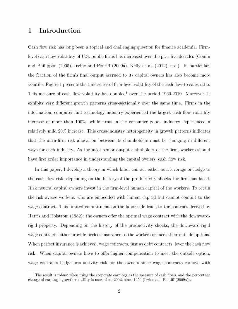
volatile. Figure 1 presents the time series of firm-level volatility of the cash flow-to-sales ratio.
This measure of cash flow volatility has doubled1 over the period 1960-2010. Moreover, it
exhibits very different growth patterns cross-sectionally over the same time. Firms in the
information, computer and technology industry experienced the largest cash flow volatility
increase of more than 100%, while firms in the consumer goods industry experienced a
relatively mild 20% increase. This cross-industry heterogeneity in growth patterns indicates
that the intra-firm risk allocation between its claimholders must be changing in different
ways for each industry. As the most senior output claimholder of the firm, workers should
have first order importance in understanding the capital owners’ cash flow risk.
In this paper, I develop a theory in which labor can act either as a leverage or hedge to
the cash flow risk, depending on the history of the productivity shocks the firm has faced.
Risk neutral capital owners invest in the firm-level human capital of the workers. To retain
the risk averse workers, who are embedded with human capital but cannot commit to the
wage contract. This limited commitment on the labor side leads to the contract derived by
Harris and Holstrom (1982): the owners offer the optimal wage contract with the downward-
rigid property. Depending on the history of the productivity shocks, the downward-rigid
wage contracts either provide perfect insurance to the workers or meet their outside options.
When perfect insurance is achieved, wage contracts, just as debt contracts, lever the cash flow
risk. When capital owners have to offer higher compensation to meet the outside option,
wage contracts hedge productivity risk for the owners since wage contracts comove with
1The result is robust when using the corporate earnings as the measure of cash flows, and the percentagechange of earnings’ growth volatility is more than 200% since 1950 (Irvine and Pontiff (2009a)).
2

1970 1975 1980 1985 1990 1995 2000 2005 2010−4.4
−4.2
−4
−3.8
−3.6
−3.4
−3.2
−3
−2.8
−2.6
−2.4
Year
Lo
g(O
pe
rati
ng
In
co
me
/Sa
les
Vo
l)
Consumer Goods
Manufacturing
Health Product
Information, Computerand Technology−NAICS
Total Average
Figure 1: Firm-Level Cash Flow Volatility
The figure reports the cash flow growth volatility at the firm level over 1960-2010. Cash flow growth is
measured by CFt−CFt−1
0.5∗Salest+0.5∗Salest−1(Bloom (2009), Jurado et al. (2013)), and cash flow is measured by
operating income (OIBDP). The standard deviation of cash flow growth is estimated over a ten-year rolling
window. The firm-level volatility is the log of the standard deviation. The figure plots the cross-firm average
of volatility within an industry. Data Source: Compustat Fundamental Annual 1960-2010.
firms’ output. The different ways in which optimal wage contracts respond to productivity
shocks drive the dynamics of risk allocation between the owners and the workers within the
firm.
The dynamics of optimal wage contract is completely capturized by two state variables:
the current human capital level and the historical maximum level of the human capital. Un-
like Harris and Holstrom (1982), due to the partial portability of firm-level human capital, the
history of productivity shocks affects the worker’s outside option through the accumulation
path of firm-level human capital. The equilibrium “effective” outside option is determined by
the firm’s historical maximum of human capital. Firms optimally offer the downward-rigid
3

wage contract to trade off between incentives and insurance. When the worker’s current
human capital level is higher than the historical maximum, causing a positive change in her
outside option, the owner benefits from retaining the current worker and raising her wage
by the smallest possible amount. With a positive wage-output sensitivity, the wage contract
acts as a “hedging” device to the owner’s cash flow risk. On the other hand, the current
human capital level can be lower than the historical maximum level, and the outside option
is lower than what the current wage contract is offering, the optimal wage contract provides
perfect insurance to the worker. With a zero wage-output sensitivity, wage contracts act as
a rigorous “debt” contract and tranfer total output into a volatile cash flow. Moreover, the
competitive equilibrium determines a concave outside option as a function of accumulated
firm-level human capital. The concavity leads to heterogeneous degrees of risk allocation
whenever a firm achieves a new historical maximum of human capital.
In the competitive equilibrium with firm dynamics, the joint distribution of wage-output
sensitivity and cash flow risk is determined by the joint distribution of current and historical
firm-level human capital accumulation. Cash flow volatility is low and wage-output sensi-
tivity is high when current human capital level exceeds the historical maximum. Cash flow
volatility is high and wage-output sensitivity is low when the worker’s current human capital
level is below the historical maximum. When wage contracts hedge the cash flow risk, firms
with a higher historical maximum of human capital have lower wage-output sensitivity and
higher cash flow volatility.
Quantitatively, the model produces predictions that are consistent with the cross-sectional
and time-series evidence on the joint distribution of cash flow volatility and wage-output sen-
sitivity. Cross-sectionally, the wage-output sensitivity explain a significant fraction of the
cross sections of the firm-level cash flow volatility. More than 50% of firm-level cash flow
volatility is explained by the changing risk sharing patterns within the firm. The calibrated
model produces the same scale of cash flow volatility variation and also matches the joint
distribution of firm-level cash flow volatility and wage-output sensitivity with the data. I
4

further evaluate the model’s implications on the driving force of the intra-firm risk sharing
dynamics. I find that the higher historical maximum of firm-level human capital predicts
(conditionally) lower wage growth and lower wage-output sensitivity, but higher cash flow
volatility. The joint distribution of the historical maximum of firm-level human capital and
cash flow volatility in the data lines up with the model prediction through the link of the
wage-output sensitivity.
In time series, the time-varying intra-firm risk allocation provides a novel explanation of
the increasing firm-level cash flow volatility. The average wage-output sensitivity decreases
38% over the period from 1960 to 2010, which suggests that workers were getting better insur-
ance in U.S. public firms over time. On average, the estimated historical maximum firm-level
human capital is growing over the same period. The historical human capital accumulation
path explains the incremental cash flow volatility through the channel of intra-firm risk al-
location. The historical maximum firm-level human capital increases most dramatically in
information, computer and technology industry, as does its average cash flow volatility at
the firm level. This industry also experiences the largest decline (more than 60%) in wage-
output sensitivity. However, in consumer goods and manufacturing industries, I didn’t find
a significant positive trend either in the historical maximum firm-level human capital or in
the average wage-output sensitivity at the industry level.
Finally, I conduct the panel analysis and confirm model’s implications in the data. I gen-
erate the following three main empirical implications: 1) a positive relationship between the
historical maximum of firm-level human capital and wage contracts; 2) a negative relationship
between compensation sensitivity and the maximal firm-level human capital conditionally; 3)
a positive relationship between cash flow volatility and maximum firm-level human capital.
The history dependence of the cross-sectional pattern of risk allocation between workers and
capital owners is sizable and significant in the data. Unconditionally, one standard deviation
increase in the historical maximum human capital level leads to a 30% change in cash flow
volatility.
5
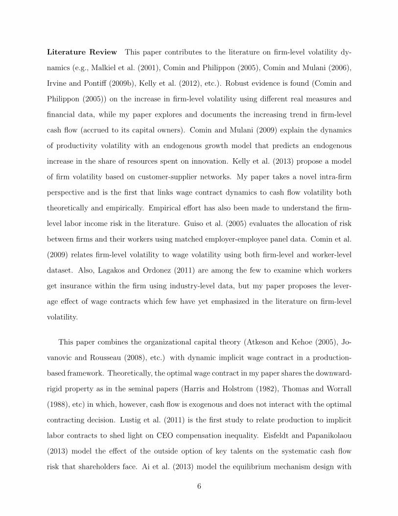
Literature Review This paper contributes to the literature on firm-level volatility dy-
namics (e.g., Malkiel et al. (2001), Comin and Philippon (2005), Comin and Mulani (2006),
Irvine and Pontiff (2009b), Kelly et al. (2012), etc.). Robust evidence is found (Comin and
Philippon (2005)) on the increase in firm-level volatility using different real measures and
financial data, while my paper explores and documents the increasing trend in firm-level
cash flow (accrued to its capital owners). Comin and Mulani (2009) explain the dynamics
of productivity volatility with an endogenous growth model that predicts an endogenous
increase in the share of resources spent on innovation. Kelly et al. (2013) propose a model
of firm volatility based on customer-supplier networks. My paper takes a novel intra-firm
perspective and is the first that links wage contract dynamics to cash flow volatility both
theoretically and empirically. Empirical effort has also been made to understand the firm-
level labor income risk in the literature. Guiso et al. (2005) evaluates the allocation of risk
between firms and their workers using matched employer-employee panel data. Comin et al.
(2009) relates firm-level volatility to wage volatility using both firm-level and worker-level
dataset. Also, Lagakos and Ordonez (2011) are among the few to examine which workers
get insurance within the firm using industry-level data, but my paper proposes the lever-
age effect of wage contracts which few have yet emphasized in the literature on firm-level
volatility.
This paper combines the organizational capital theory (Atkeson and Kehoe (2005), Jo-
vanovic and Rousseau (2008), etc.) with dynamic implicit wage contract in a production-
based framework. Theoretically, the optimal wage contract in my paper shares the downward-
rigid property as in the seminal papers (Harris and Holstrom (1982), Thomas and Worrall
(1988), etc) in which, however, cash flow is exogenous and does not interact with the optimal
contracting decision. Lustig et al. (2011) is the first study to relate production to implicit
labor contracts to shed light on CEO compensation inequality. Eisfeldt and Papanikolaou
(2013) model the effect of the outside option of key talents on the systematic cash flow
risk that shareholders face. Ai et al. (2013) model the equilibrium mechanism design with
6

limited commitment to explain the inequality in CEO compensation. In contrast, I explore
the endogenous relationship between organization capital accumulation and the wage con-
tract stickiness. My paper also contributes to the empirical literature on wage structure
at the firm level. Baker et al. (1994) use an employee-employer matched database for a
single firm and find that employees are partly shielded against changes in external market
conditions. Wachter and Bender (2007) find the persistent cohort effect on wages within the
firm. Beaudry and DiNardo (1991) show that there is a time-varying degree of risk sharing
between workers and firms at the time of entry. My model implications are consistent with
the empirical evidence on wage structure in the existing literature, and provides additional
insights into the second moment of wage structure.
This paper is related to both the empirical and theoretical corporate finance literature
that focuses on the optimal compensation scheme and the interaction between financial
decisions and agency frictions (e.g., He (2011), Demarzo et al. (2012)). I study dynamic
wage contracts with limited commitment, similar to Berk et al. (2010), to generate the
labor-induced operating leverage effect. Different from Berk et al. (2010), where the amount
of risk sharing between investors and employees depends on the debt level, the degree of risk
sharing in my paper depends on the high-water mark of human capital reached in the firm’s
entire history. Michelacci and Quadrini (2009) study the long-term wage contract in the
financially constraint firms and find a positive relationship between firm size and wages. My
model produce predictions consistent with Michelacci and Quadrini (2009) but with emphasis
on implications for wage-output sensitivity and cash flow volatility. There is rising attention
on labor in empirical corporate finance. Garmaise (2008) and Benmelech et al. (2011) among
others, study the interaction between firms’ employment decisions and financial frictions.
Tate and Yang (2013) estimate the labor market consequences of corporate diversification
using worker-firm matched data. My paper suggests implications concerning the inefficiency
of human capital investment at the firm level and provides a novel link between corporate
investment and labor compensation. Related to the empirical work starting with Jensen and
7

Murphy (1990), my model produces a stickier performance-pay wage contract that survives
the empirical tests.
This paper also incorporates several successful themes from the emerging literature that
examines the relation between labor frictions and risk and asset returns. Berk and Walden
(2013) studies the limited capital market participation as an equilibrium outcome in the
neoclassical asset pricing model, where firms offer labor contracts that insure workers who
then optimally choose not to participate in capital markets. My paper assumes exogenous
nonparticipation in the capital markets and focuses on the implications for intra-firm risk
sharing. The leverage effect of wage stickiness has been shown by Danthine and Donaldson
(2002), Favilukis and Lin (2012) and Favilukis and Lin (2013), who document the importance
of labor leverage in explaining equity premium. In a competitive labor market setting, Gourio
(2008) shows the empirical implications of sticky wages for the cross-sectional differences in
return as well. Donangelo (2013) studies that labor mobility amplifies the firms’ existing
exposure to systematic risk. In my paper, I emphasize the heterogeneity in the corporate
rent-splitting and endogenize the elasticity of wage to output by the implicit wage contracts.
Eisfeldt and Papanikolaou (2013) also explore the division of surplus between key talent and
shareholders with the accumulation of organizational capital. In their paper, the dynamics
of the rent splitting depend on the current level of frontier technology, but not on the
historical accumulation path of organization capital. The unmeasured capital is also modeled
in Jovanovic and Rousseau (2008) with an emphasis on the managerial function of assembling
heterogeneous assets. The specificity of human capital creates rents in the assembly in
Jovanovic and Rousseau (2008), but their model does not imply the division of rents between
different claimholders of the firm.
8
2 The Model
I construct an competitive industry equilibrium model in the tradition of Hopenhayn (1992)
and Gomes (2001), augmented with human capital and implicit labor contract. I start with
a simple version of the model that features only human capital accumulation and production
to illustrate the key dynamics of cash flows and wage contracts.
2.1 The Environment
The production economy consists of two sectors: capital owners and workers. A continumm
of firms is owned by risk neutral capital owners who have limited liability, while a continumm
of workers is risk averse and cannot participate in the financial market2 and have no access
to a storage technology. Both the owners and the workers have the same discount factor β.
The labor contract is the only source of consumption smoothing for the risk averse agent.
2.1.1 Firm Behavior
Production requires two inputs, capital ht and labor lt, and is subject to an idiosyncratic
technology shock, zt ∼ Q(zt|zt−1):
yt = eztf(ht, lt). (1)
The production function f(·) is well-defined3 and displays decreasing return to scale. The
output is homogeneous. Assumption 1 and 2 concern the nature of the productivity shock.
Assumption 1 (a) The stochastic process for the idiosyncratic shock z has bounded support
Z = [z, z], −∞ < z < z < ∞; (b) the idiosyncratic shocks follow a common stationary and
2Berk and Walden (2013) studies the limited participation in the capital markets as an optimal equilibriumoutcome in a production economy.
3Production is carried out under the well-defined space, which is strictly increasing, strictly concave, twicecontinuously differentiable, homogeneous, and constant return to scale, and satisfies Inada conditions.
9

increasing Markov transition function Q(zt|zt−1) that satisfies the Feller property; (c) the
productivity shock zt is independent across firms.
For the sake of simplicity, I normalize the overall labor force of the firm equal to one
(lt = 1); hence human capital ht can be interpreted as the productivity per worker. An
active firm is equivalent to a match of capital ht and one worker. The space of capital
input is a subset of the non-negative bounded real numbers, H ∈ [hmin,∞), and hmin ∈ R is
the general human capital (e.g., education) embodied in the worker at the beginning of the
match. The match-level human capital is ht ∈ H. The accumulation law of capital ht+1 for
the next period follows the traditional investment function It:
It = ht+1 − (1− δh)ht, δh ∈ (0, 1), (2)
where δh is the depreciation rate of human capital.
The match-level human capital accumulation is not completely exclusive to the worker.4
Unlike the standard neoclassical investment model, this paper emphasizes the sharing prop-
erty of match-level human capital.
Assumption 2 (Portability) The fraction of match-level human capital φht is portable
with the worker when the separation of capital and labor happens, 0 < φ < 1.
Due to the partial portability of human capital, the capital is most efficient in the match
where it was accumulated, although it can also be partially adopted by other firms (φ < 1).
I summarize the firm’s decision by first writing down the cash flow process:
CFt = eztf(ht)− wt − Iht − s, (3)
where s is the fixed production cost for each period. Each firm maximizes the discounted
cash flow stream over its life cycle: E0[∑∞
s=t βs−tCFs|z0)].
4For example, the “skill-weights” view suggested by Lazear (2009).
10

2.1.2 Labor Market
A continuum of workers are risk averse and infinitely-lived. Each period, workers consume
their wages, but they have limited commitment to the wage contracts. Workers can al-
ways walk away whenever an outside option is higher than the contract provided by the
match. The owners have full commitment to the wage contracts, but with limited liabil-
ity. Owners commit to a complete contingent optimal contract at the start of the match
{wt(zt), ηt(zt)}τt=0, where zt denotes the history of shocks, zt = {zt, zt−1, ...}, ηt is an indica-
tor function that governs the optimal decision of dissolving the match, and τ is the optimal
time of termination. Here, for tractability, I assume that the contingent optimal contract
cannot be negotiated ex post.5
Subject to Assumption 2, the labor mobility cost between firms is captured by 1 − φ,
where φ is an exogenous parameter and may vary across industries, so the optimal wage
contract must be self-enforcing. I provide a simple characterization of the optimal contract
following Thomas and Worrall (1988), but with an endogenous equilibrium outside option.
The optimal contract maximizes the total expected payoff of the owner, subject to deliv-
ering initial utility ϕ0 to the workers:
ϕ0(z0) = E0[∞∑0
βtu(wt(zt))].
To make the problem recursive, the worker’s promised expected utility is treated as a new
state variable. The optimal contract delivers ϕt today by delivering current wage wt and
a state-contingent promised expected utility ϕt+1 tomorrow. The owners commit to deliver
{wt, ϕt+1(zt+1, ht+1, ηt+1)} each period, where ϕt+1(zt+1, ht+1, ηt+1) is defined as:
ϕt(zt, ht, ηt) = Et[∞∑s=t
βs−tu(ws(zs, hs, ηs))]. (4)
5In some states where the match is terminated, the contract does leave room for renegotiation as long asthe turnover is also costly for the worker (φ < 1).
11
The domain of feasible promised utility Φ = [ϕ, ϕ] is defined in Appendix A.1. The capital
owners have to keep their promises by setting up the following promise-keeping constraint:
ϕt = u(wt) + β
∫ηt+1ϕt+1Q(dzt+1|z) + β
∫(1− ηt+1)ϕres,t+1Q(dzt+1|z). (5)
Given workers’ limited commitment and the partial portability of match-level human capital,
the optimal contract should provide retention incentives. Let ϕres,t+1 denote the workers’
reservation utility, which is defined as the outside option of the workers; thus, the contingent
promised utility has to be higher than ϕres,t+1 for any realized state at t+1. The participation
constraint of the workers is given by:
ϕt+1 ≥ ϕres,t+1(φht+1, zt+1, ηt+1), ∀zt+1 ∈ Z , ∀ht+1 ∈ H. (6)
The contract offers as high as the worker’s outside option, which is an equilibrium outcome
from firm dynamics.
2.1.3 Exit, Entry and Firm Dynamics
The entry and exit of the firm is defined as the formation and termination of the capital-labor
match respectively. The timing of firms’ entry and exit decision is shown in Figure 2.
In any given period, the owner of each incumbent firm decides whether to exit or stay
before the shock (zt+1) is observed (see Gomes (2001)). Hence, incumbents know in advance
whether or not to exit in the next period, and the exit is completely determined by the
current productivity shock zt. The indicator variable ηt+1 is one if continuation is optimal
and zero otherwise:
ηt+1 =
1, if zt ≥ max[z∗t , z]
0, otherwise,
(7)
12
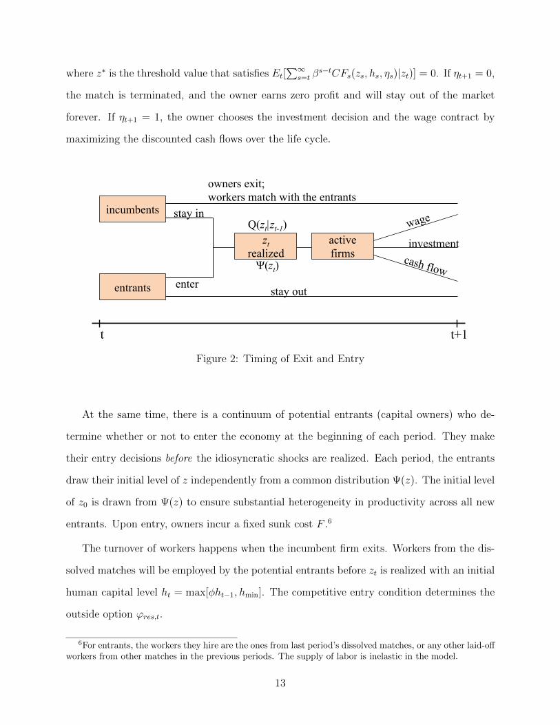
where z∗ is the threshold value that satisfies Et[∑∞
s=t βs−tCFs(zs, hs, ηs)|zt)] = 0. If ηt+1 = 0,
the match is terminated, and the owner earns zero profit and will stay out of the market
forever. If ηt+1 = 1, the owner chooses the investment decision and the wage contract by
maximizing the discounted cash flows over the life cycle.
t t+1
incumbents
entrants
active firms
zt realized
owners exit; workers match with the entrants
stay out
stay in
enter
wage
investment cash flow
Q(zt|zt-1)
Ψ(zt)
Figure 2: Timing of Exit and Entry
At the same time, there is a continuum of potential entrants (capital owners) who de-
termine whether or not to enter the economy at the beginning of each period. They make
their entry decisions before the idiosyncratic shocks are realized. Each period, the entrants
draw their initial level of z independently from a common distribution Ψ(z). The initial level
of z0 is drawn from Ψ(z) to ensure substantial heterogeneity in productivity across all new
entrants. Upon entry, owners incur a fixed sunk cost F .6
The turnover of workers happens when the incumbent firm exits. Workers from the dis-
solved matches will be employed by the potential entrants before zt is realized with an initial
human capital level ht = max[φht−1, hmin]. The competitive entry condition determines the
outside option ϕres,t.
6For entrants, the workers they hire are the ones from last period’s dissolved matches, or any other laid-offworkers from other matches in the previous periods. The supply of labor is inelastic in the model.
13

2.2 The Firm’s Optimization Problem
If the capital-labor match dissolves, the owner realizes zero value forever. Hence, the interest-
ing case that remains is the optimal compensation and investment decision of the incumbent
firms.
The dynamic formulation of each incumbent firm’s problem can be written in a recursive
form in which the state variables are {h, ϕ, z} ∈ H×Φ× Z and subject to constraints from
capital accumulation and labor market friction. Define V (h, ϕ; z) as the value of a firm that
has a capital stock of h, promised utility to the worker ϕ, and productivity z. Both owners
and workers discount the future by a common factor β. Given ηt+1 = 1, the dynamic problem
P facing the owner of each incumbent is:
V (h, ϕ; z) = maxht+1,ϕt+1,w;zt+1|z
(CFt + β
∫V (ht+1, ϕt+1; zt+1)Q(dzt+1|z)
)(8)
subject to:
CFt = exp(zt)f(ht)− wt − It, (9)
It = ht+1 − (1− δh)ht, δh ∈ (0, 1), (10)
ϕt = u(wt) + β
∫ϕt+1Q(dzt+1|z), (11)
ϕt+1 ≥ ϕres,t+1(φht+1, zt+1), ∀ht+1 ∈ H, ∀zt+1 ∈ Z. (12)
Constraint (9) is the budget constraint for the capital owner; constraint (10) is the law of
motion of human capital; and constraint (11) is the promise-keeping constraint. Since the
incumbent has made the decision regarding ηt+1 before solving P, constraint (11) is the
version of equation (5) with ηt+1 = 1. The participation constraint (12) is contingent on the
endogenous state ht+1. This is the main difference from the literature on the risk-sharing
contract with one-sided commitment. The model allows for dynamic contracting to interact
with the firm’s investment behavior. The more the firm invests, the higher the worker’s
14

outside option as the firm grows.
The limited commitment on the part of workers and the endogenous exit decision com-
plicate the dynamic programming considerably. However, I show that there exists a unique
solution to problem P characterized in the Lemma 1 and 2.
Lemma 1 Given the outside option ϕres(φh) ∈ [ϕ, ϕ], the solution V (h, ϕ, z) to the Bell-
man equation P exists. The value function is strictly monotone, concave, continuous and
differentiable in ϕ and h.
Proof. See Appendix A.2.
Lemma 2 Given the initial ϕ0, the optimal contract {wt, ϕt+1} and policy function of h is
unique and continuous.
Proof. See Appendix A.2. The risk averse worker is willing to accept a lower expected
wage in exchange for a smoother income stream. The capital owner can make a profit by
paying a wage lower than the competitive wage when the productivity shock is positive and
vice versa. This is an implicit leverage effect generated by the self-enforcing wage contract.
The leverage effect consists of two parts. (1) Since the contract wage will be lower than the
competitive spot market wage, more room for profit is left to the capital owners; (2) the wage
will be stickier than the competitive market wage, and the stickiness is history-dependent.
The intra-firm risk allocation is governed by the strength of the implicit leverage effect.
2.3 Aggregation and Equilibrium
In the competitive equilibrium, free entry stipulates that the equilibrium value of a new
match of labor and capital is equal to the entry cost:
∫Vt(φht, ϕres(φht), z)Ψ(dz) ≤ F. (13)
15
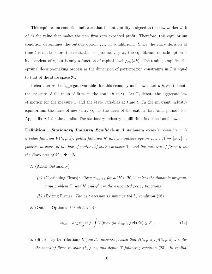
This equilibrium condition indicates that the total utility assigned to the new worker with
φh is the value that makes the new firm zero expected profit. Therefore, this equilibrium
condition determines the outside option ϕres in equilibrium. Since the entry decision at
time t is made before the realization of productivity zt, the equilibrium outside option is
independent of z, but is only a function of capital level ϕres(φh). The timing simplifies the
optimal decision-making process as the dimension of participation constraints in P is equal
to that of the state space H.
I characterize the aggregate variables for this economy as follows. Let µ(h, ϕ, z) denote
the measure of the mass of firms in the state (h, ϕ, z). Let Γt denote the aggregate law
of motion for the measure µ and the state variables at time t. In the invariant industry
equilibrium, the mass of new entry equals the mass of the exit in that same period. See
Appendix A.1 for the details. The stationary industry equilibrium is defined as follows.
Definition 1 Stationary Industry Equilibrium A stationary recursive equilibrium is
a value function V (h, ϕ, z), policy function h′ and ϕ′, outside option ϕres : H → [ϕ, ϕ], a
positive measure of the law of motion of state variables Υ, and the measure of firms µ on
the Borel sets of H × Φ× Z:
1. (Agent Optimality)
(a) (Continuing Firms): Given ϕres,t+1 for all h′ ∈ H, V solves the dynamic program-
ming problem P, and h′ and ϕ′ are the associated policy functions.
(b) (Exiting Firms): The exit decision is summarized by condition (26).
2. (Outside Option): For all h′ ∈ H:
ϕres ∈ argmaxϕ{ϕ|
∫V (max[φh, hmin], ϕ)Ψ(dz) ≤ F}. (14)
3. (Stationary Distribution) Define the measure µ such that ∀(h, ϕ, z), µ(h, ϕ, z) denotes
the mass of firms in state (h, ϕ, z), and define Υ following equation (23). In equilib-
16

rium,
(Υ, µ) = H(Υ, µ).
The following proposition summarize the equilibrium properties.
Proposition 1 The stationary equilibrium exists and the equilibrium outside option is strictly
increasing and concave in h.
Proof. See Appendix A.4.
The nonlinearity of the outside option gives a very distinct impulse response to the
productivity shocks, given different human capital accumulation paths. The heterogeneous
degree of risk sharing between workers and capital owners arises endogenously across firms.
3 Equilibrium Risk Allocation
Perfect consumption-smoothing breaks with limited commitment and firm dynamics. In
this section, I describe the heterogeneous degree of stickiness of the wage contracts in the
equilibrium. Two state variables summarize all necessary information for risk sharing in
equilibrium: the current level of human capital ht and the historical maximal level of human
capital: hmax,t−1 = max{hs−1, s = 1...t}.
3.1 Optimal Wage Contract
Given the existence of the equilibrium, I first characterize the dynamics of the wage contract
in Proposition 2.
Proposition 2 (Downward-Rigidity) Given the initial wage contract {w0, ϕ0} and zt ≥
max[z∗, z], the maximum of human capital hmax,t = max{hs, s ≤ t} is the sufficient statistic
of the equilibrium wage.
17

Proof. See Appendix A.4.
As in Harris and Holstrom (1982), proposition 2 implies that only the maximum level
of ht impacts the wage level as long as the firm stays in the economy. hmax,t governs how
much the capital owner needs to transfer to the worker in the optimal contract, and the wage
contract is reset whenever hmax,t > hmax,t−1.
The perfect risk sharing wage contract provides smooth consumption over time ( 1u′(wt)
=
1u′(wt+1)
), and the lagged inverse marginal utility (LIMU), 1u′(wt)
, contains the only rele-
vant information in forecasting next period’s wage level, wt+1. When perfect consumption-
smoothing is constrained by limited commitment, LIMU is no longer sufficient to determine
the next period’s wage. The Euler equation is obtained under limited commitment:
1
u′(wt+1)=
1
u′(wt)− θt(ht+1), (15)
where θt(·) is the Lagrangian multiplier of the participation constraint (12). Conditional only
on θt(·), the shadow price of the promised utility at time t+1, LIMU is sufficient for predicting
the next period’s wage level. The wage contract is reset to the higher level whenever the
participation constraint is binding; it remains at the same level when the participation
constraint is not binding. The shadow price of the promised utility θt(·) becomes positive
only when workers’ outside option rises. Given that the outside option is an increasing
function of h from Proposition 1, the maximum level of human capital hmax,t contains all the
information relevant for forecasting the wage contract in the next period.
With limited commitment on the labor side, the optimal contract should move as little
as possible to trade off between the marginal value of retention incentives and the marginal
benefit of consumption smoothing. Figure 3(a) illustrates the equilibrium wage contract.
Whenever the productivity shock zt+1 induces a positive increase in hmax,t+1, the participation
constraint binds and the marginal value of increasing ϕt+1 rises and dominates the marginal
value of insurance. The firm increases the promised value ϕt+1 to retain the worker in the
18
match. The optimal contract depends only on the current state of the firm. Although it
is costly for the firm to increase ϕt+1, it benefits the firm from the marginal productivity
of the worker. However, when the productivity shock zt+1 leads to disinvestment at t + 1
and ht+1 < hmax,t+1, the worker’s participation constraint is loosened and the optimal wage
contract stays constant. As long as ht+1 < hmax,t+1, the marginal value of smoothing the
worker’s consumption dominates, and perfect insurance is achieved. The wage contract is
completely captured by the maximum level of the human capital stock in the firm’s history
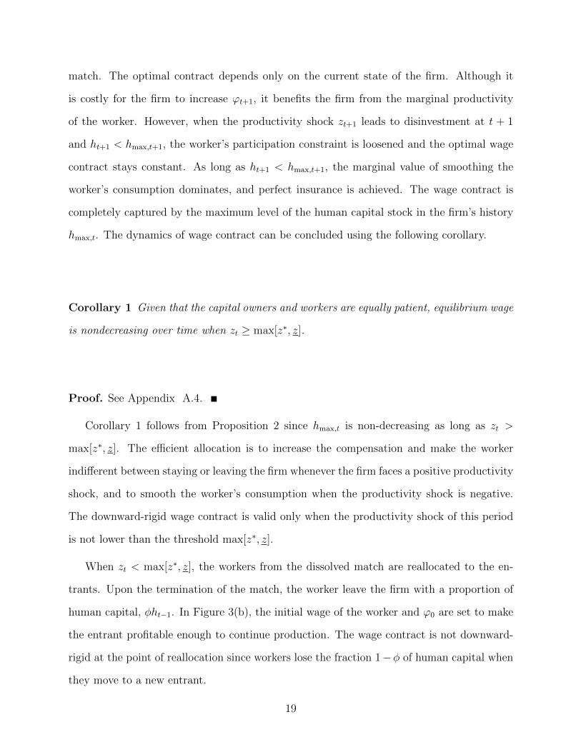
hmax,t. The dynamics of wage contract can be concluded using the following corollary.
Corollary 1 Given that the capital owners and workers are equally patient, equilibrium wage
is nondecreasing over time when zt ≥ max[z∗, z].
Proof. See Appendix A.4.
Corollary 1 follows from Proposition 2 since hmax,t is non-decreasing as long as zt >
max[z∗, z]. The efficient allocation is to increase the compensation and make the worker
indifferent between staying or leaving the firm whenever the firm faces a positive productivity
shock, and to smooth the worker’s consumption when the productivity shock is negative.
The downward-rigid wage contract is valid only when the productivity shock of this period
is not lower than the threshold max[z∗, z].
When zt < max[z∗, z], the workers from the dissolved match are reallocated to the en-
trants. Upon the termination of the match, the worker leave the firm with a proportion of
human capital, φht−1. In Figure 3(b), the initial wage of the worker and ϕ0 are set to make
the entrant profitable enough to continue production. The wage contract is not downward-
rigid at the point of reallocation since workers lose the fraction 1−φ of human capital when
they move to a new entrant.
19

(a) Optimal Wage Contract Before Exit
0 5 10 15 20 25 30 35 40−10
−5
0
5
10
15
Period
z_t
wage
h_max
h
(b) Optimal Wage Contract With Exit
0 10 20 30 40 50 60 70 80 90−15
−10
−5
0
5
10
15
20
25
Period
z_t
wage
h_max
h
exit
Figure 3: Wage Contract and Human Capital
This figure plots the wage contract and its dynamics with respect to the human capital accumulation path.
Figure (a) shows the wage contract dynamics before the termination of the match. Figure (b) shows the wage
contract and the exit-and-entry dynamics, where the grey area indicates the termination of the capital-labor
match. The unit of productivity shock zt is scaled up ten times.
20

3.2 History-Dependent Risk Allocation in Equilibrium
In equilibrium, the outside option drives the optimal rent-splitting rule between workers and
capital owners, and the sensitivity of the outside option to the productivity shocks differs
across firms. The important question before moving on to cash flow volatility is the relative
risk-sharing magnitude in equilibrium and its cross-sectional distribution. The equilibrium
property of workers’ outside option directly implies the following corollary:
Corollary 2 Given ϕ0, zt < max[z∗, z], and the concavity of ϕres(h) from Proposition 1,
∂ϕt
∂h1t≥ ∂ϕt
∂h2tif h1
t ≤ h2t .
Concavity of the outside option in the human capital level implies a difference in sensitiv-
ity of the promised utility on the maximum level of the human capital accumulation. As the
maximum of the human capital level gets higher, the promised utility becomes less respon-
sive to the productivity shock and, hence, the consumption. However, when the historical
maximum of human capital level is low, the worker gets better insured from the productivity
shock, and the wage contract is less responsive. The equilibrium distribution of wage to
output sensitivity is consistent with the equilibrium distribution of hmax.
Figure 9 shows the impluse response function of cash flows and wage contracts subject to
a one-standard deviation shock. Consider two firms with the same starting level of ϕ0 and
human capital ht level, but with a different history of human capital accumulation hmax,t.
With high hmax,t, the firm offers a wage contract that is less responsive to productivity
shocks (both positive and negative), while with low hmax,t, the firm offers a wage contract
that is more sensitive to productivity shocks. When the wage contract is less sensitive,
compensation to the worker is relatively smooth and acts as leverage to the owner’s cash
flow and firm value. When the wage contract fluctuates with respect to the productivity
shocks, the cash flow and the firm value become smoother since the compensation hedges
against the productivity risk for the capital owner.
21

3.3 Labor as Hedge or Leverage?
Allowing the endogenous outside option produces the equilibrium joint distribution of wage
contract dynamics and cash flow volatility. The wage contract can act either as a hedge
against productivity shocks or as leverage for the owner’s cash flow. Also, the leverage and
hedge effect differs across firms, depending on the historical maximum level of human capital
and the current human capital level. I define hthmax,t−1
as the distance between the current
capital level and the running maximum level of the human capital, hmax,t−1.
Proposition 3 Given ϕ0 and w0, hmax,t and hthmax,t−1
are the only relevant state variables
that impact wage contract dynamics.
Proof. The dynamics are captured by the tightness of the participation constraint. Given
the monotonicity of ϕres(h) in equilibrium, the Proposition is straightforward.
The role of labor in the firm is governed by hthmax,t−1
. I first define the wage-output
sensitivity βw,y = β∆w,∆y of wage growth on output growth as a measure of the degree of
risk sharing in equilibrium. When hthmax,t−1
is greater than one, investment responds to the
significant positive productivity shock, and firms optimize the total value by taking advantage
of the better investment opportunity and committing to higher labor costs. Both the wage-
output sensitivity is then positive, βw,y > 0. The wage contract acts as a hedge to the cash
flow risk. Labor acts as leverage to the cash flow and βw,y = 0 when hthmax,t−1
≤ 1, since the
wage contract is downward-rigid. The productivity risk is allocated optimally between the
capital owner and the worker conditional on hthmax,t−1
. The wage contract provides insurance to
the worker for small positive and negative shocks, but not for large positive shocks. The state
variable hthmax,t−1
has the same feature as all the dynamic contracts with limited commitment,
e.g.,(Thomas and Worrall, 1988),(Kocherlakota, 1996),(Krueger and Uhlig, 2006), except
that, here, the state variable hthmax,t−1
is from an endogenous decision.
A nice intuition behind the state variable hthmax,t−1
is the average Q value of the firm (as
in Lustig et al. (2011)). The market-to-book ratio is defined as q = MB
= V (h,ϕ,z)h
. When
22

hthmax,t−1
is low, for a given level ht, a higher hmax,t−1 indicates that the worker is compensated
with higher rent according to the optimal wage contract, so V (h, ϕ, z) is lower and, hence,
V (h,ϕ,z)h
is low. Low market-to-book ratio firms are low hthmax,t−1
firms. On the one hand, firms
with a low market-to-book ratio are firms that have a higher historical maximum capital
level, hmax,t−1, and tend to provide better insurance to their workers. On the other hand,
high market-to-book ratio firms have a relatively lower running maximum level of historical
human capital, so they share less rent with workers, and the owners of the firms bear less
productivity risk. Workers act more like leverage in the low market-to-book ratio firms, but
act more like a hedge in the high market-to-book ratio firms.
hthmax,t−1
≤ 1 hthmax,t−1
> 1
β∆w,∆y = 0 Low β∆w,∆y
High hmax,t High Leverage HedgeHigh σ(∆CF ) Median σ(∆CF )β∆w,∆y = 0 High β∆w,∆y
Low hmax,t Low Leverage HedgeMedian σ(∆CF ) Low σ(∆CF )
Table 1: Equilibrium Joint Distribution of βw,y and σ(∆CF )
The historical running maximum of human capital, hmax, determines how the corporate
rent created by the match of capital and labor is split between these two claimholders. When
labor acts as leverage to the cash flow risk, hmax governs the difference in the leverage ratio.
When labor acts as a hedge on productivity risk for the owners, hmax controls the difference
in the magnitude of risk that the wage contract helps offset.
The dynamics of the wage contracts are characterized jointly by hthmax,t−1
and hmax,t. The
joint distribution of sensitivity of wage growth on output growth, βw,y, and cash flow volatility
in equilibrium lines up with the joint distribution of hthmax,t−1
and hmax,t in equilibrium (Table
1).
Figure 4 shows the dynamics of sensitivity and volatility with respect to the change of
hthmax,t−1
and hmax,t before the match dissolves. The wage-output sensitivity is increasing in
23

hthmax,t−1
and decreasing in hmax,t. When hthmax,t−1
≤ 1, wage growth responds little to output
growth and wage-output sensitivity stays close to zero. When hthmax,t−1
≥ 1, wage gets less
sensitive and less responsive to output as hmax,t gets higher. The dynamic risk allocation
is consistent with the cash flow volatility dynamics: the better the consumption smoothing
provided to the worker, the more risk the capital owner bears.
(a) Risk Allocation: Sensitivity
0 5 10 15 20 25 30 35 40 45−0.5
0
0.5
1
1.5
2
2.5
3
period
Sensitivity
h/h_max
h_max
β(∆ wage,∆ y)
β(∆ CF,∆ y)
(b) Risk Allocation: Volatility
0 5 10 15 20 25 30 35 40−0.5
0
0.5
1
1.5
2
2.5
3
period
Volatility
h/h_max
h_max
σ(∆ wage)
σ(∆ CF)
σ(∆ CF/y)
Figure 4: Risk Allocation in Equilibrium
This figure shows the equilibrium risk allocation in the simulated economy. Cash flow-output sensitivity
and wage-output sensitivity are measured by the regression coefficient of cash flow/wage growth on the
output growth ∆y. I estimate the regression coefficient the volatility σt at time t using ten periods (forward)
simulated data points.
The policy function of a numerical excercise in Figure 8 shows wage-output sensitivity
and cash flow volatility as the function of h and ϕ implied by the model. To facilitate the
quantitative analysis, Figure 8 shows the policy for the volatility of cash flows scaled by
output (CFy
). The result is preserved when cash flow is scaled by output. Since hmax is
the sufficient statistic for the worker’s promised utility ϕ, the policy function illustrates the
dynamics of wage-output sensitivity and cash flow volatility with respect to h and hmax.
The volatility of cash flow increases in hmax because of the leverage effect, but decreases in
h. The reason why cash flow volatility decreases in h in the policy function is as follows.
When h exceeds hmax, wage contracts comove with the human capital level h and act as
24

hedges, so cash flow volatility remains at a low level; when h is lower than hmax, the implicit
wage contract becomes effective leverage, hence cash flow volatility is high. The wage-output
sensitivity increases with respect to h, but decreases with respect to hmax. In the bottom
panel (left picture), wherever wage-output sensitivity hits zero, the value of promised utility
ϕ implies the value of hmax equal to h, and as hmax (ϕ) increases, the sensitivity is equal to
zero. Higher wage-output sensitivity is obtained when h is higher than hmax.
4 Quantitative Results
This section presents the quantitative results of the stationary industry equilibrium. Com-
puting the equilibrium requires the specification of the functional forms and determination
of the parameter values. Because the exact analytical solution is impossible to obtain under
this framework, the computational procedure is provided in Appendix B.
4.1 Measurement and Data Construction
One of the key features of the model is that it generates the distribution of firm-level human
capital and the evolution of firm-level human capital accumulation. Measuring human capital
or intangible capital has a long history in the economics literature. The conceptual and
measurement approach depends on my theoretical predictions as well as the availability of
firm-level data.
4.1.1 Defining and Measuring Firm-Level Human Capital
The key variable h that governs the risk allocation dynamics is firm-level human capital:
human capital that is accumulated along with production. Different from the standard
definition of human capital (general skill of labor), firm-level human capital has more overlap
with the intangible assets of the firm in both accounting terms and qualitative properties.
Borrowing from the definition of intangible assets in Brynjolfsson et al. (2002), I focus on
25

a firm’s intellectual assets and innovation, as well as its organizational structure (including
information technology and computer expenses).
According to the existing literature (Corrado et al. (2004), Lev and Radhakrishnan
(2005), Hulten and Hao (2008), Eisfeldt and Papanikolaou (2013), Falato et al. (2013), etc.),
in the Compustat database, the computerized information (including organizational struc-
ture, etc.) and the economic competencies (knowledge embedded in firm-specific human and
structural resources, including brand names) are recognized as a fraction of Selling, General
and Administrative (SG&A) expenses, and the corresponding line for innovative property
is R&D expenses. I attribute 30% of SG&A outlays7 plus R&D expenses to labor-related
intangible spending. All the investment spending is deflated by the production price index
from NIPA.
To obtain the firm-level human capital stock, I start with the estimates of real investment
spending and apply the perpetual inventory method ht+1 = (1−δh)ht+Ih. I need two further
elements to implement the capital accumulation method: a depreciation rate δh and the
capital benchmark h0. Relatively little is known about depreciation rates for human capital.
I borrow the depreciation rate estimated by Corrado et al. (2006) for all three categories of
intangible assets. The initial capital stock, h0, for each category is set to the same amount
of capital spending as that of the first year available in the Compustat database divided
by depreciation rate. The assumption of the initial stock value and depreciation rate is not
crucial for the result since I am more interested in the relative position of firm-level human
capital stock than in its quantitative value. For a robustness check, I use the total SG&A
expenses as labor-related investment at the firm level, and I also exclude R&D expenses from
our firm-level human capital investment estimates. The quantitative result remains robust
in general.
7The labor-related items account for 10% to 70% of the SG&A expenses (from 10-K fillings of publicfirms). In Hulten and Hao (2008), 30% is applied to capture the investment in organizational developmentand worker training. I use 30% here to follow the general guidance of Corrado et al. (2006)’s macro research.
26

4.1.2 Variables Construction
State Variable Construction
Given the calculation of firm-level human capital stock hi,t, the measure of hmax,it is con-
structed in two ways.
First, I measure hmax,it by taking the maximum of the whole history (available in the
data). Although there are missing data before IPO, I assume that the first available obser-
vation captures that history.
Second, I construct hmax,it by computing the value-weighted average of the past N -year
firm-level human capital stock, ht−N+1, ..., ht. Also for robustness, I define a dummy variable
dh,t = 1 if ht−i > ht−i+1, and impose the weight in that year, wi,t = 0. This measure helps
to smooth out the noise by taking a moving weighted average of the historical capital stock,
but it also rules out the data points where the depreciation of human capital is dominant. I
drop the estimates whenever there is a missing observation in the N-year horizon. h is scaled
by the physical capital level given by gross property, plant, and equipment (PPEGT) item
from Compustat.
Other Variables
The firm-level wage-output sensitivity βw,y is computed by running a ten-year rolling window
regression of the per capita wage growth on the growth of per capita value-added. The
regression is conducted for each firm, and I record the panel of the regression coefficients
βw,y,it.
The sample includes all the U.S. public firms in CRSP-Compustat merge file frim 1960-
2010. For consistency, I include firms with fiscal year ending month in December (fyr=12),
firms with non-missing SIC codes, firms with non-negative value of sales and firms with
non-missing SG&A expenses. The details in the data sources, as well as the definition and
construction of other variables can be found in Appendix C. All the firm characteristics and
target moments for parameter choices are summarized in Table 8.
27

4.2 Benchmark Parameter Choices
Given the availability of firm-level public firm accounting data, I calibrate all the parameters
of the model at an annual frequency to match the standard macroeconomic moments and
firm dynamics.
Preference For convenience, I assume that employees are endowed with CRRA utility
with a constant risk-aversion coefficient equal to 2 (γ = 2). The time preference parameter
β is set to 0.96, which implies an annual risk-free rate of 4%. I calibrate the model to match
interest rate at a relatively higher level since the model does not have implications for the
risk premium; 4% is the average of long-term risk premium and the 30-day U.S. Treasury
bill return.
Technology Assume that production takes place in each firm according to a decreasing
returns-to-scale Cobb-Douglas production function, yt = ezthαt . The parameter α is drawn
randomly from [0.78, 0.86]. The range of human capital intensity is set to match the average
labor share jointly with φ. The output y and firm-level human capital h are both scaled by
physical capital k.
The idiosyncratic productivity shocks are uncorrelated across firms and have a common
stationary and monotonic Markov transition function, denoted by Qz(zt|zt−1) as zt = ρzzt−1+
σzεt. The parameters ρz and σz are calibrated to match the unconditional second moments
and first-order autocorrelation of firm-level TFP shocks. ρz and σz are also chosen to match
the degree of persistence and the dispersion in the equilibrium distribution of firms, so I
restrict their value to ρz = 0.7 and σz = 0.3. The new entrants draw the initial productivity
level z0 from a uniform distribution over the same finite support Z as the incumbents. See
Appendix B.3 for details.
The rate of depreciation in human capital is set to equal 0.2.8 I also assume it is costly to
adjust firm-level human capital in the calibration with the convex adjustment cost g(h, I) =
8A six-year write-off of human capital is suggested by Corrado et al. (2004).
28

Table 2: Benchmark Calibration
Parameter Symbol ValueHuman capital intensity α 0.78-0.86Human capital depreciation rate δh 0.2Symmetric investment adjustment cost ξh 3.2Persistent coefficient of idiosyncratic productivity ρz 0.7Conditional volatility of idiosyncratic productivity σz 0.3Time preference β 0.96Constant risk-aversion coefficient (CRRA utility) γ 2Portability of human capital φ 0.5Production cost s 0.08
The table presents the calibration parameter choice for the benchmark model. The parameters are either
estimates from empirical studies or calibrated to match a set of key moments in the model to the U.S. data
at an annual frequency. See Appendix B.3.
12ξh(
Ih)2h. The convexity parameter ξh is set to 3.2 assuming a similar adjustment time of
human capital from the empirical evidence (See Appendix B.3).
Labor Market There is little suggested evidence of φ in the data, and it’s reasonable
to believe that φ should vary across firms and over time. The parameters φ and α are
calibrated to determine the labor share. In the benchmark calibration, I set φ = 0.5 to
match the labor share 0.43 in U.S. public firms, since the major focus in this paper is on
equilibrium distribution of human capital accumulation.
Entry and Exit The choice of fixed sunk cost s and entry cost F should be calibrated
to match the entry and exit rate, respectively. The Compustat dataset provides an unbal-
anced panel with significant firm turnover. In the model, the match turnover dynamics are
essentially skilled labor turnover at the micro level, so I calibrate the values to match the
the plant-level exit and entry rate 6.2% found in the literature (e.g., Clementi and Palazzo
(2010)).
Table 2 summarizes the key parameter values used in solving and simulating the baseline
model.
29

4.3 Calibration Results
Table 3: Key Moments Under Baseline Parameterization
Target Moments Model Data
Panel A: TechnologyTFP persistency AR(1) 0.7 0.7σ(TFP ) 0.43 0.42
Panel B: Human Capital (h)Standard Deviation 2.55 2.59Skewness 1.70 2.82Investment to Capital (h) Ratio 0.21 0.23Investment to Revenue Ratio 0.28 0.18
Panel C: Labor Sharewageoutput
0.49 0.43
The table presents key moments generated by the model baseline parameterization compared to the data
moments. All the second moments reported above are unconditional. The investment to revenue ratio is the
ratio of investment in organizational capital devided by net sales. The data source of firm-level cash flow and
investment characteristics is from Compustat fundamental annual: 1960-2010 and Eisfeldt and Papanikolaou
(2013). The data source of firm-level TFP is from Imrohoroglu and Tuzel (2011).
The model is solved numerically with all the details of solving the firm’s optimization
problem and the outside option in the industrial equilibrium in the Appendix B. I then
simulate the economy with N firms over T periods using the optimal decision rule and value
function. Set N = 3000 and T = 300 and repeat the simulation in a large number of times.
The first 100 periods is discarded to make sure the convergence of the “simulated economy”.
Panel A, B and C in Table 3 contain the key moments that the model is calibrated
to match under benchmark parameterization. The parameters are chosen to match the
distribution of firm-level human capital and TFP shocks. Table 4 provides the results of
matching the data moments at the aggregate level. The model produces lower wage growth
(log) volatility −1.48 than cash flows growth volatility −0.09, which is close to the cash flow
growth volatility in the data. The cash flow-output sensitivity is greater than one since the
30
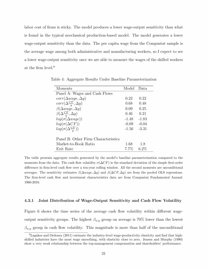
labor cost of firms is sticky. The model produces a lower wage-output sensitivity than what
is found in the typical neoclassical production-based model. The model generates a lower
wage-output sensitivity than the data. The per capita wage from the Compustat sample is
the average wage among both administrative and manufacturing workers, so I expect to see
a lower wage-output sensitivity once we are able to measure the wages of the skilled workers
at the firm level.9
Table 4: Aggregate Results Under Baseline Parameterization
Moments Model DataPanel A: Wages and Cash Flowscorr(∆wage,∆y) 0.22 0.22corr(∆CF
y,∆y) 0.68 0.48
β(∆wage,∆y) 0.09 0.25β(∆CF
y,∆y) 0.46 0.21
log(σ(∆wage)) -1.48 -1.83log(σ(∆CF )) -0.09 -0.04log(σ(∆CF
y)) -1.56 -3.31
Panel B: Other Firm CharacteristicsMarket-to-Book Ratio 1.68 1.8Exit Rate 7.7% 6.2%
The table presents aggregate results generated by the model’s baseline parameterization compared to the
moments from the data. The cash flow volatility σ(∆CF ) is the standard deviation of the simple first-order
difference in firm-level cash flow over a ten-year rolling window. All the second moments are unconditional
averages. The sensitivity estimates β(∆wage,∆y) and β(∆CF,∆y) are from the pooled OLS regressions.
The firm-level cash flow and investment characteristics data are from Compustat Fundamental Annual:
1960-2010.
4.3.1 Joint Distribution of Wage-Output Sensitivity and Cash Flow Volatility
Figure 6 shows the time series of the average cash flow volatility within different wage-
output sensitivity groups. The highest βw,y group on average is 70% lower than the lowest
βw,y group in cash flow volatility. This magnitude is more than half of the unconditional
9Lagakos and Ordonez (2011) estimate the industry-level wage-productivity elasticity and find that high-skilled industries have the most wage smoothing, with elasticity close to zero. Jensen and Murphy (1990)show a very weak relationship between the top-management compensation and shareholders’ performance.
31
standard deviation (1.30) of cash flow volatility in the whole sample. In fact, in the highest
βw,y quantile, the cash flow volatility trends downward over time.
Table 5 shows the cash flow volatility of different wage-output sensitivity groups. The
wage-output sensitivity βw,y is estimated using the regression coefficient of wage growth and
output growth over a ten-period10 rolling window for each firm in the simulated economy. I
also obtain estimates of firm-level cash flow volatility over the same window. All the firms
are sorted into three groups based on βw,y. The simulation is repeated 100 times. Table 5
reports the cross-simulation averages for each group.
Table 5 Panel B shows that there is a spread of 70% in cash flow volatility (among
different wage-output sensitivity groups). The model also produces about 60% difference in
cash flow volatility between highest βw,y group and the lowest βw,y group. The change in
degree of insurance provided to the workers within the firm is correlated with the change in
the firm-level cash flow volatility and hence the return volatility.
The model captures the joint distribution of wage dynamics and cash flow volatility in
the data. Panel B of Table 5 shows a strong positive relationship between βw,y and cash flow
volatility and a positive relationship between βw,y and firm-level stock return volatility. The
fact that the cash flow volatility spread between the highest β group and the lowest is the
same as the wage volatility spread indicates that the variation in cash flow volatility is due
to the variation in wage contract sensitivity. The wage leverage is more effective and stickier
in the low βw,y group, where firm-level cash flow growth is more volatile. One exception is
that the model does not generate the same magnitude of stock return volatility, since the risk
premium and stochastic discount factor are not modeled here. However, the stock return
volatility across βw,y groups decreases with respect to βw,y, and the difference in volatility
between the highest and the lowest βw,y groups is about 15% in the data.
10I apply both five-period and fifteen-period window to estimate the wage-output sensitivity, the result isrobust in general.
32

Table 5: Volatility of Portfolios Sorted on β(∆w,∆y)
Panel A: Model Portfolio Volatility
Group (β∆w,∆y) log(σ∆wage) log(σret) log(σ∆CFy
) log(σ∆CF )
low -3.37 -0.85 -1.17 0.51median -2.66 -0.97 -1.38 0.19high -2.46 -1.11 -1.77 -0.23
Panel B: Data Portfolio Volatility
Group(β∆w,∆y) log(σ∆wage) log(σret) log(σ∆CFy
) log(σ∆CF )
low -2.30 -3.69 -3.38 0.31median -2.26 -3.72 -3.55 -0.19high -1.81 -3.84 -4.08 -0.52
This table presents the volatility of wages and cash flows for the β(∆w,∆y) sorted portfolios.CFy is the
operating income scaled by sales. The volatility is in terms of log and is annualized. The volatility is
computed within a ten-year rolling window and average across firms within the group. The cash flow
volatility σ(∆CF ) is the standard deviation of the simple first-order difference in firm-level cash flow over
a ten-year rolling window. The stock return volatility is computed using CRSP daily stock returns, and
I derive the stock return volatility using observations within each year and then annualize the volatility
estimates. Panel A reports the results from the simulation based on the benchmark choice of parameters.
Panel B reports the results from the historical data (1960-2010).
4.3.2 Joint Distribution of State Variables and Cash Flow Volatility
I now show the empirical results that support the model mechanism and the consistent
transitory dynamics of the state variables with cash flow volatility and the wage-output
sensitivity. Two main predictions are obtained regarding the joint distribution of state
variables and key second moments from both Corollary 2 and Proposition 3. First, the
higher the maximal level of human capital, the lower is the wage sensitivity conditional on
hthmax,t−1
> 1; second, the higher the maximal level of human capital, the higher is the cash
flow volatility unconditionally.
Table 6 shows the portfolio cash flow volatility and portfolio wage-output sensitivity for
different hmax groups conditional on hthmax
from the data. In Panel A, cash flow volatility
increases with hmax unconditionally, with a 90% difference between high hmax group and low
hmax group. In Panel B, there is also consistent evidence that βw,y is lower when hmax gets
33

Table 6: 3 Portfolios Sorted by State Variables (Data)
Panel A: log(σ(CFy
)) Panel B: β(∆w,∆y)ht
hmax,t−1
hthmax,t−1
Group(hmax) ≤ 1 > 1 Total ≤ 1 > 1 Totallow -3.47 -3.37 -3.44 0.30 0.32 0.30
median -3.06 -3.00 -3.04 0.12 0.11 0.12high -2.55 -2.58 -2.56 0.09 0.10 0.09
This table presents the cash flows (CFy ) growth volatility and wage-output sensitivity for the hmax-sorted and
ht
hmax,t−1-sorted portfolios. Both the standard deviation and the sensitivity are computed within a ten-year
rolling window and averaged across firms within the group. The volatility is the log of the standard deviation
and is annualized. Data Source: Compustat Fundamental Annual: 1960-2010.
Table 7: 3 Portfolios Sorted by State Variables (Model)
Panel A: log(σ(CFy
)) Panel B: β(∆w,∆y)
hthmax,t−1
hthmax,t−1
Group(hmax) ≤ 1 > 1 Total ≤ 1 > 1 Totallow -1.62 -1.66 -1.65 0.03 0.06 0.03
median -1.22 -1.21 -1.21 0.008 0.01 0.01high -1.13 -1.19 -1.18 -0.15 -0.25 -0.16
This table presents the cash flow (CFy ) growth volatility and wage-output sensitivity estimated from the
simulated economy using the benchmark calibration. The exact same procedure of estimation is conducted
in the simulated economy. The standard deviation and sensitivity β are computed within a ten-period rolling
window and averaged across firms within the group. The volatility is in terms of log.
higher. In terms of predicting cash flow growth volatility, hthmax
does not play a significant role.
Conditional on hthmax
> 1, cash flow growth volatility is on average higher, while the model
predicts less risk allocated to the owners because part of the volatility is absorbed by the
wage contract. The data do not show a strong effect of hthmax
, mainly because over time there
is a positive trend in ht. In most of the sample period, hthmax
is a number slighly above 1. In
terms of model evaluation, the simulated economy also generate a reasonable distribution of
cash flow growth volatility (see Table 7). The average cash flow volatility in the highest hmax
group is 47% higher than the lowest hmax group. The group with hhmax
> 1 does not produce
a much lower cash flow volatility than the group with hhmax
≤ 1 due to the way I estimate
34

the second moments. Cash flow volaitlity and wage-output sensitivity are both estimated
over a ten-period rolling window, so hhmax
> 1 at period t does not gurantee that hhmax
> 1 in
the following nine periods within the window. Wage-output sensitivity is higher on average
in the group with hhmax
> 1, and there is a 0.21 spread between high hmax group and the low
hmax group. In the high βw,y group, the negative βw,y comes from workers ’s turnover and
the negative growth of output when the firm has a high-water mark of human capital. For
the same reason as I match the aggregate moments, the model produces a relatively lower
wage-output sensitivity than the data.
4.4 Increasing Cash Flow Volatility 1960-2010
Knowing how risk is allocated between capital and labor within the firm not only helps us
to understand the cross sections of cash flow volatility, but also provides a novel explanation
for the time-varying firm-level cash flow volatility. Capital owners of U.S. public firms bear
more and more risk over the past few decades (Comin and Philippon (2005), Comin et al.
(2009) and Kelly et al. (2012),etc.). Table 9 provides the key measure of intra-firm risk-
sharing dynamics over different periods. On average, hmax, cash flow growth volatility and
wage growth volatility (i.e., firm-level volatility) all increase at the firm level, but within the
firm, the wage-output sensitivity decreases 41% (Figure 5). The average U.S. public firms
have become more and more human capital intensive and have provided better insurance to
their workers over time (Figure 5).
As shown in Figure 5, risk allocation between labor and capital owners presents dif-
ferent patterns across industries. The industries with high hmax in equilibrium have lower
wage sensitivity to output growth. Even industries that are currently experiencing positive
productivity shocks have little flexibility in adjusting compensation since their production
technologies rely heavily on human capital. If we look at the intra-firm risk allocation dy-
namics of different industries, the average wage-output sensitivity trends downward (Figure
5(b)), with information, computer and technology industry declining the most. In manufac-
35

(a) Industry hmax
1965 1970 1975 1980 1985 1990 1995 2000 2005 20100
0.5
1
1.5
2
2.5
3
3.5
4
4.5
5
5.5
Year
H_m
ax
Manufacturing
Consumer Goods
Health Products
Information, Computerand Technology−NAICS
Total Average
(b) Industry β(∆w,∆y)
1960 1965 1970 1975 1980 1985 1990 1995 2000 20050.2
0.3
0.4
0.5
0.6
0.7
0.8
0.9
1
Year
β(∆
w,∆
y)
Manufacturing
Consumer Goods
Health Products
Information, Computerand Technology−NAICS
Total Average
Figure 5: Time Series Historical Maximum of Firm-Level Human Capital and Wage-OutputSensitivity
The figure shows the time series of historical maximum of firm-level human capital and wage-output sensi-
tivity for different industries. The maximum human capital level hmax is measured by the value-weighted ht
over the past five years and scaled by the physical capital stock over the same period. The wage-output sen-
sitivity at the industry level is the average of wage-output sensitivity estimates of firms within the industry.
Sample period: 1960-2010.
turing and consumer goods, where cash flow volatility increased mildly before the 1980s, the
firm-level human capital accumulation is relatively stable.
The secular rise in intangible capital is well-documented in macroeconomics and finance
literature11. Since hmax has increased over time, I conduct a comparative-static excercise to
see whether the model converges to a different equilibrium cash flow volatility by varying
the human capital intensity parameter in the production function. Figure 13(a) shows that
equilibrium h distribution with different α values leads to heterogeneous cash flow volatility
and wage-output sensitivity, which is highly consistent with the time series moments in
Figure. 13(b).
As shown in Figure 12(b), the fraction of firms with hthmax,t−1
lower than one increases over
time, while hthmax,t−1
decreases over time, but on average is above one. The average firm in the
11Jovanovic and Rousseau (2008) emphasize the rise in firm specificity of human capital as a result of thegrowth of product variety. Falato et al. (2013) explores the rise in intangible assets as a fundamental driverof the secular trend in U.S. corporate cash holdings over the past few decades.
36

market exhibits growth in firm-level human capital, implying that there is improvement in
risk sharing at the firm-level. The ratio of the current human capital level to the historical
maximal human capital level is relevant for this explanation. The ratio tends to be above
one, on average, before 1980, and then decreases after 1980. The maturity indicates a high
inflexibility in the labor sector of a firm, which creates a strong leverage effect on the firm’s
cash flow.
4.5 Empirical Evidence From Panel Analysis
As additional empirical examination of my theory, I conduct the panel analysis and confirm
the model’s implications using actual data. There are three key implications from the theory:
1) a positive relationship between the historical maximum of firm-level human capital and
wage contracts; 2) a negative relationship between compensation sensitivity and the maximal
firm-level human capital conditional on hthmax,t−1
> 1; 3) a positive relationship between cash
flow volatility and maximal firm-level human capital unconditionally.
4.5.1 Wage Contract and hmax
First, wage level is predicted by hmax,t controlling for current productivity shocks and other
firm characteristics. The prediction is tested as follows:
wageit = α + ηi + λt + β1hmax,it + β2TFPit + ΓXit + εit, (16)
where Xit is a vector of control variables, including market-to-book ratio, net sales, and
market capitalization. The results are shown in Table 10 and Table 11 as the robustness
check. Wage is measured using per capita labor expenses from Compustat dataset (wage
I) or using per capita labor expenses with the missing total labor expenses replaced by per
capita SG&A (wage II). See Appendix C for details. Table 10 shows the regression results
using the direct measure of hmax. The dependent variable is log(wage I) in the columns (1)
37

and (2) and is log(wage II) in the columns (3) and (4). Controlling for the current TFP
level, hmax is positively correlated with wage level (β1 > 0). The result also holds when the
historical maximum TFP level is used as the measure of the historical maximum of firm-level
human capital accumulation. Table 11 reports the regression results using the value-weighted
measure of hmax,vw (see Appendix C).
The effect of the historical maximum of firm-level human capital on the average real wage
is statistically significant and sizeable. Controlling for the current productivity level, a one
standard deviation12 change in hmax accounts for a 22% increase in the firm-level average real
wage. Workers are compensated by firms’ historical investment in human capital. Over the
period from 1960 to 2010, the maximum of accumulated human capital has increased 267%
(about one standard deviation, see Table 9), while the average real wage at the firm level
has increased by an average of 85%. The historical maximum of firm-level human capital
indicates an increase of greater than 25% in the average real wage in the sample.
4.5.2 Risk Allocation and Firm-Level Human Capital Investment
The model has direct implications for how wage contracts respond to output growth, condi-
tional on the history of firm-level human capital. Wage-output sensitivity is positive when
the firm hits a new running maximum of human capital, hmax, but wage-output sensitivity
is negatively correlated with maximal firm-level human capital conditional on hthmax,t−1
> 1.
I first conduct a regression of wage growth on dummy D(hmax,it > hmax,it−1) = 1
if hmax,it > hmax,it−1, controlling for output growth, and adding the interaction term of
D(hmax,it > hmax,it−1) and output growth:
∆wageit = α + ηi + λt + β1D(hmax,it > hmax,it−1) + β2∆y + β3(Dummy ×∆y) + ΓXit + εit.(17)
Wage growth is the difference in the log average real wage of each firm. As shown in
the regression results in Table 12, the output growth is proxied by using labor productivity
12The standard deviation of log(hmax) is 1.35.
38

growth (column (1)-(2)) and value-added growth (column (3)-(4)). Robust results are ob-
tained by changing the measures for output. The wage growth is positive when firms invest
in their firm-level human capital (β1 > 0), and is significantly positively correlated to output
growth. With a one standard deviation increase in labor productivity growth, wage growth
increases (on average) 11.5%, contributing to 55% of the wage growth standard deviation.
This result is consistent with the average labor share in U.S. public firms. The regression
coefficient is negative in the interaction term, which is also aligned with the model’s predic-
tions. When firms increase their human capital accumulation, the sensitivity of wage growth
to labor productivity growth declines. The following regression is needed to help explain the
magnitude of this finding:
∆wageit = α + ηi + λt + β1hmax,it + β2∆y + β3(hmax,it ×∆y) + ΓXit + εit. (18)
A negative regression coefficient β3 means that hmax increases, the wage-output sensitivity
declines. In the subsample hthmax,t−1
> 1, β3 is significantly negative (Table 14, column (2)). A
one standard deviation increase in hmax absorbs 8% of the wage-output sensitivity, which is
13% of a standard deviation of βw,y. The negativity of β3 is robust to the change of measure
of ∆y (Table 14, column (4)). In the subsample where hthmax,t−1
≤ 1, β3 is either non-negative
or insignificant. Table 13 reports the results using wage (I) as the dependent variables. All
results remain robust, except for the significant negative β3 when using ∆tfp as the measure
of ∆y.
4.5.3 Cash Flow Volatility and Human Capital Accumulation
Finally, I examine whether the model’s implication for cash flow volatility is also confirmed
in the data. I test the positive correlation between cash flow volatility and historical human
capital accumulation in the subsample where hthmax,t−1
≤ 1, and then compare the results with
39

the results where hthmax,t−1
> 1.
σ(∆CF ) = α + ηi + λt + β1hmax,it + ΓXit + εit. (19)
Regression results are shown in Table 15. Cash flow volatility is significantly negatively
correlated with hmax. In column (3) when hthmax,t−1
≤ 1, hmax predicts a higher cash flow
volatility than when hthmax,t−1
> 1. Unconditionally, a one standard deviation increase in hmax
leads to a 30% change in cash flow volatility. When hthmax,t−1
≤ 1, the leverage effect of human
capital is amplified and leads to 50% increase in cash flow volatility. Over the sample period
from 1960 to 2010, firm-level hmax has increased by about one standard deviation, which
predicts a 30% change in cash flow volatility on average. This result seems to underestimate
the incremental size of cash flow volatility, but the intra-firm channel dominates other firm
characteristics in predicting change in cash flow risk. I also check equity return volatility
as a measure of firm-level cash flow risk. I find that equity return volatility is positively
correlated with hmax, but this significant positive correlation is found only in the sample
where hthmax,t−1
≤ 1. The labor “leverage” effect is stronger than the size effect from column
(1).
5 Conclusion
Who bears more risk within the firm? It depends on the current and historical human capital
of the firm. On the one hand, wage contracts can serve as a hedging device to the capital
owner’s cash flow risk when the firm has a higher current level of human capital than its
historical maximum. On the other hand, wage contracts can behave like debt and leverage
the cash flow risk when the historical level of human capital is higher than the current level.
To understand the heterogeneous roles of labor in the firm, I develop a theory in which
the optimal wage contract and the optimal investment decision are both endogenously de-
termined in equilibrium. This paper is the first to generate the joint distribution of cash
40

flow volatility and wage-output sensitivity. Empirically, my predictions from the model line
up with the cross-sectional and time series evidence in the data. The intra-firm risk alloca-
tion channel explains more than 50% of the cash flow volatility variation in the data. Over
time, the decline in wage-output sensitivity coincides with the increase in firm-level cash flow
volatility.
The intra-firm labor frictions bring a novel perspective to understanding the firm-level
risk. Firms have invested more and more in the workers over the past few decades. This
paper shows that investing in human capital can be potentially more costly than investing in
physical capital. Better understanding of the endogenous investment cost on human capital
and its implications for asset returns is an important part of the future research.
41
References
Abowd, John M., John Haltiwanger, Ron Jarmin, Julia Lane, Paul Lengermann,Kristin McCue, Kevin McKinney, and Kristin Sandusky, “The Relation amongHuman Capital, Productivity, and Market Value: Building Up from Micro Evidence,” in“Measuring Capital in the New Economy” NBER Chapters, National Bureau of EconomicResearch, Inc, 2005, pp. 153–204.
Ai, Hengjie, Dana Kiku, and Rui Li, “A Mechanism Design Model of FirmDynamics: The Case of Limited Commitment,” July 2013. Available at SSRN:http://ssrn.com/abstract=2347821.
Atkeson, Andrew and Patrick J. Kehoe, “Modeling and Measuring Organization Cap-ital,” Journal of Political Economy, October 2005, 113 (5), 1026–1053.
Baker, George, Michael Gibbs, and Bengt Holmstrom, “The Wage Policy of a Firm,”The Quarterly Journal of Economics, November 1994, 109 (4), 921–55.
Beaudry, Paul and John DiNardo, “The Effect of Implicit Contracts on the Movement ofWages over the Business Cycle: Evidence from Micro Data,” Journal of Political Economy,August 1991, 99 (4), 665–88.
Benmelech, Efraim, Nittai K. Bergman, and Amit Seru, “Financing Labor,” NBERWorking Papers 17144, National Bureau of Economic Research, Inc., June 2011.
Berk, Jonathan B. and Johan Walden, “Limited Capital Market Participation andHuman Capital Risk,” Review of Asset Pricing Studies, April 2013, 3 (1), 1–37.
, Richard Stanton, and Josef Zechner, “Human Capital, Bankruptcy, and CapitalStructure,” Journal of Finance, June 2010, 65 (3), 891–926.
Bloom, Nicholas, “The Impact of Uncertainty Shocks,” Econometrica, May 2009, 77 (3),623–685.
Brynjolfsson, Erik, Loren Hitt, and Shinkyu Yang, “Intangible Assets: How theInteraction of Computers and Organizational Structure Affects Stock Market Valuations,”Brookings Papers on Economic Activity, 2002, 33 (1), 137–198.
Clementi, Gian Luca and Dino Palazzo, “Entry, Exit, Firm Dynamics, and AggregateFluctuations,” Working Paper Series 27-10, The Rimini Centre for Economic Analysis,January 2010.
Comin, Diego and Sunil Mulani, “Diverging Trends in Macro and Micro Volatility,”Review of Economics and Statistics, May 2006.
and , “A theory of growth and volatility at the aggregate and firm level,” Journal ofMonetary Economics, November 2009, 56 (8), 1023–1042.
42

and Thomas Philippon, “The Rise in Firm-Level Volatility: Causes and Conse-quences,” NBER Working Papers 11388, National Bureau of Economic Research, Inc.,May 2005.
, Erica L. Groshen, and Bess Rabin, “Turbulent firms, turbulent wages?,” Journalof Monetary Economics, January 2009, 56 (1), 109–133.
Corrado, Carol A., Charles R. Hulten, and Daniel E. Sichel, “Intangible Capitaland Economic Growth,” NBER Working Papers 11948, National Bureau of EconomicResearch, Inc., January 2006.
Corrado, Carol, Charles Hulten, and Daniel Sichel, “Measuring capital and technol-ogy: an expanded framework,” Finance and Economics Discussion Series 2004-65, Boardof Governors of the Federal Reserve System (U.S.) 2004.
Danthine, Jean-Pierre and John B Donaldson, “Labour Relations and Asset Returns,”Review of Economic Studies, January 2002, 69 (1), 41–64.
Demarzo, Peter M., Michael J. Fishman, Zhiguo He, and Neng Wang, “DynamicAgency and the q Theory of Investment,” Journal of Finance, December 2012, 67 (6),2295–2340.
Donangelo, Andres, “Labor Mobility: Implications for Asset Pricing,” Journal of Finance,Forthcoming, May 2013.
Eisfeldt, Andrea L. and Dimitris Papanikolaou, “Organization Capital and the Cross-Section of Expected Returns,” The Journal of Finance, Feburary 2013, 68 (4), 1365 –1406.
Falato, Antonio, Dalida Kadyrzhanova, and Jae Sim, “Rising Intangible Capital,Shrinking Debt Capacity, and the US Corporate Savings Glut,” Technical Report, FEDSWorking Paper No. 2013-67 September 2013.
Favilukis, Jack and Xiaoji Lin, “Does Wage Rigidity Make Firms Riskier? Evidencefrom Long-Horizon Return Predictability,” Working Paper Series 2012-19, Ohio StateUniversity, Charles A. Dice Center for Research in Financial Economics, October 2012.
and , “Wage Rigidity: A Quantitative Solution to Several Asset Pricing Puzzles,” July2013. Fisher College of Business Working Paper No. 2012-03-016; Charles A. Dice CenterWorking Paper No. 2012-16. Available at SSRN: http://ssrn.com/abstract=2141275.
Garmaise, Mark J., “Production in Entrepreneurial Firms: The Effects of Financial Con-straints on Labor and Capital,” Review of Financial Studies, April 2008, 21 (2), 543–577.
Gomes, Joao F., “Financing Investment,” American Economic Review, December 2001,91 (5), 1263–1285.
Gourio, Francois, “Labor Leverage, Firms Heterogeneous Sensitivities to the BusinessCycle, and the Cross-Section of Returns,” 2008 Meeting Papers 149, Society for EconomicDynamics, 2008.
43

Guiso, Luigi, Luigi Pistaferri, and Fabiano Schivardi, “Insurance within the Firm,”Journal of Political Economy, October 2005, 113 (5), 1054–1087.
Hall, Robert E., “The Stock Market and Capital Accumulation,” American EconomicReview, December 2001, 91 (5), 1185–1202.
Harris, Milton and Bengt Holstrom, “A Theory of Wage Dynamics,” Review of Eco-nomic Studies, July 1982, 49 (3), 315–33.
He, Zhiguo, “A model of dynamic compensation and capital structure,” Journal of Finan-cial Economics, May 2011, 100 (2), 351–366.
Hopenhayn, Hugo A, “Entry, Exit, and Firm Dynamics in Long Run Equilibrium,”Econometrica, September 1992, 60 (5), 1127–50.
Hulten, Charles and Janet Hao, “Intangible Capital and the Market to Book ValuePuzzle,” Economics Program Working Papers 08-02, The Conference Board, EconomicsProgram, June 2008.
Imrohoroglu, Ayse and Selale Tuzel, “Firm Level Productivity, Risk, and Return,”2011 Meeting Papers 21, Society for Economic Dynamics, 2011.
Irvine, Paul J. and Jeffrey Pontiff, “Idiosyncratic Return Volatility, Cash Flows, andProduct Market Competition,” Review of Financial Studies, March 2009, 22 (3), 1149–1177.
and , “Idiosyncratic Return Volatility, Cash Flows, and Product Market Competition,”Review of Financial Studies, March 2009, 22 (3), 1149–1177.
Jensen, Michael C and Kevin J Murphy, “Performance Pay and Top-ManagementIncentives,” Journal of Political Economy, April 1990, 98 (2), 225–64.
Jovanovic, Boyan and Peter L. Rousseau, “Specific Capital and Technological Variety,”NBER Working Papers 13998, National Bureau of Economic Research, Inc., May 2008.
Jurado, Kyle, Sydney C. Ludvigson, and Serena Ng, “Measuring Uncertainty,”NBER Working Papers 19456, National Bureau of Economic Research, Inc., September2013.
Kelly, Bryan T., Hanno N. Lustig, and Stijn Van Nieuwerburgh, “The VolatilityFactor Structure,” November 2012. Chicago Booth Research Paper No. 12-54; Fama-MillerWorking Paper.
, , and , “Firm Volatility in Granular Networks,” NBER Working Papers 19466,National Bureau of Economic Research, Inc., September 2013.
Kocherlakota, Narayana R, “Implications of Efficient Risk Sharing without Commit-ment,” Review of Economic Studies, October 1996, 63 (4), 595–609.
44

Koop, Gary, M. Hashem Pesaran, and Simon M. Potter, “Impulse response analysisin nonlinear multivariate models,” Journal of Econometrics, September 1996, 74 (1), 119–147.
Krueger, Dirk and Harald Uhlig, “Competitive risk sharing contracts with one-sidedcommitment,” Journal of Monetary Economics, October 2006, 53 (7), 1661–1691.
Lagakos, David and Guillermo L. Ordonez, “Which workers get insurance within thefirm?,” Journal of Monetary Economics, September 2011, 58 (6), 632–645.
Lazear, Edward P., “Firm-Specific Human Capital: A Skill-Weights Approach,” Journalof Political Economy, October 2009, 117 (5), 914–940.
Lev, Baruch and Suresh Radhakrishnan, “The Valuation of Organization Capital,” in“Measuring Capital in the New Economy” NBER Chapters, National Bureau of EconomicResearch, Inc.,, July 2005, pp. 73–110.
Lustig, Hanno, Chad Syverson, and Stijn Van Nieuwerburgh, “Technological changeand the growing inequality in managerial compensation,” Journal of Financial Economics,March 2011, 99 (3), 601–627.
Malkiel, Burton, John Campbell, Martin Lettau, and Yexiao Xu, “Have IndividualStocks Become More Volatile? An Empirical Exploration of Idiosyncratic Risk,” Journalof Finance, 02 2001, 56 (1), 1–43.
Michelacci, Claudio and Vincenzo Quadrini, “Financial Markets and Wages,” TheReview of Economic Studies, 2009, 76 (2), 795–827.
Olley, G Steven and Ariel Pakes, “The Dynamics of Productivity in the Telecommuni-cations Equipment Industry,” Econometrica, November 1996, 64 (6), 1263–97.
Shapiro, Matthew D, “The Dynamic Demand for Capital and Labor,” The QuarterlyJournal of Economics, August 1986, 101 (3), 513–42.
Tate, Geoffrey and Liu Yang, “The Bright Side Of Corporate Diversification: EvidenceFrom Internal Labor Markets,” Working Papers 13-40, Center for Economic Studies, U.S.Census Bureau., August 2013.
Thomas, Jonathan and Tim Worrall, “Self-enforcing Wage Contracts,” Review of Eco-nomic Studies, October 1988, 55 (4), 541–54.
von Wachter, Till and Stefan Bender, “Do initial conditions persist between firms? :an analysis of firm-entry cohort effects and job losers using matched employer-employeedata,” IAB Discussion Paper 200719, Institut fr Arbeitsmarkt- und Berufsforschung (IAB),Nrnberg [Institute for Employment Research, Nuremberg, Germany] June 2007.
Whited, Toni M, “Debt, Liquidity Constraints, and Corporate Investment: Evidence fromPanel Data,” Journal of Finance, September 1992, 47 (4), 1425–60.
45
A Technical Appendix
A.1 Aggregation
Technical Assumptions(a) The space of input is a subset of the (non-negative) bounded real numbers, H ∈ [hmin,∞)and hmin ∈ R. The stochastic process for the idiosyncratic shock z has bounded supportZ = [z, z], −∞ < z < z < ∞; (b) the idiosyncratic shock follows a common stationary andincreasing Markov transition function Q(zt|zt−1) that satisfies the Feller property; (c) theproductivity shock zt is independent across firms; (d) each period, the entrants draw theirinitial level of z independently from a common distribution Ψ(z); (e) the domain of feasiblepromised utility, Φ = [ϕ, ϕ].
Naturally, ϕ is the lifetime discounted utility of a worker in the firm with the highesthuman capital accumulation:13
ϕ = max{wt}∞0
∞∑t=0
βtu(wt), (20)
subject to:
∞∑t=0
βtwt ≤ W (h),
where W (h) = y(h,z)1−β + β
∑z′ π(z′|z)y(h, z′) is the present discounted social output.
Symmetrically, I can define the lower bound of promised utility to the worker by pickingan arbitrary small positive w > 0 (smaller than the marginal product of l at hmin, and defineϕ = u(w) as the lifetime utility from consuming the lowest possible income forever. Notethat the boundary is loose enough that the equilibrium ϕ might not hit either the lower orthe upper bound.
AggregationDefine the measure µ such that ∀(h, ϕ, z) ∈ H×Φ× Z, µ(h, ϕ, z) denotes the mass of firmsin the state (h, ϕ, z) and Θ = H × Φ× Z. The law of motion of the state variable dependson the transition function from agents’ optimality, but the invariant distribution of mass ofthe firm µ is determined by the exit-entry decision.
Let κ be an indicator function defined by the policy function for the promised utility andhuman capital:
κ(h′, ϕ′, z′;h, ϕ, z) =
{1, if ϕ′(h′, ϕ′, z′;h, ϕ, z) = ϕ′ & h′(h′, ϕ′, z′;h, ϕ, z) = h′,
0, elsewhere.(21)
13h, the existence of h < h∗ is guaranteed by the decreasing return to scale production function.
46

I can then define the transition function Λ for Θ:
Λ((h′, ϕ′, z′), (h, ϕ, z)) = Q(z′|z)κ(h′, ϕ′, z′;h, ϕ, z). (22)
I use Υt to denote a positive measure of the law of motion of state variables at time t. Itslaw of motion is implied by the transition function Λ:
Υt+1(h′, ϕ′, z′) =
∫ ∞hmin
∫ ϕ
ϕ
∫ z
z
Λ((h′, ϕ′, z′), (h, ϕ, z))µt(h, ϕ, z)dΘt, (23)
where µt(h, ϕ, z) is the measure of surviving firms in period t:
µt(h, ϕ, z) =
∫ ∞hmin
∫ ϕ
ϕ
∫ z
z
η(k, ν, a)dΛ(k, ν, a). (24)
In the invariant industry equilibrium, the mass of new entry equals the mass of the exitin that same period:
µ′(h′, ϕ′, z′) =
{Λ((h′, ϕ′, z′), (h, ϕ, z))µ(h, ϕ, z), if ϕ ≤ ϕ∗
Λ((h′, ϕ′, z′), (h, ϕres(h), z))µ(h, ϕres(h), z), if ϕ > ϕ∗.(25)
A.2 Proof of Lemma 1 and Lemma 2
This is the standard proof following Stockey, Lucas and Prescott (1989).
Proof of Lemma 1. (Existence.) First, I show that the constraint set is non-empty. Thevalue function is a mapping from a set of bounded and continuous functions C(H×Φ×Z) toC(H×Φ×Z). Second, I show that value function is a contraction in C(H×Φ×Z). A standardcontraction mapping theorem implies that there is a unique fixed point in C(H × Φ × Z),and ensures the existence, strict monotonicity, and concavity of V .
(Monotonicity.) From Lemma 9.5 and Corollary 1 of Theorem 3.2 in Stokey, Lucas andPrescott (1989), it is straightforward that V (h, ϕ, z) is strictly increasing in h and z, andstrictly decreasing in ϕ.
(Concavity.) To prove that V (h, ·, z) is strictly concave, I first consider some h and ϕ1 6=ϕ2 and, for each ϕi, consider a stochastic sequence of optimal choice (yt,i, ϕt,i, zt,i, wt,i)|∞t=0
from iterating the solution to the dynamic programming problem forward, starting withh0,i = h and ϕ0,i = ϕi. Given the boundedness, per iteration gives:
ϕi = (1− β)E[∞∑0
βtu(wt,i)].
A similar iteration for V (h, ϕ) yields:
V (h, ϕi) = E[∞∑0
βtdt,i].
47

Consider now the convex combination ϕλ = λϕ1 + (1− λ)ϕ2. A feasible plan is given bythe convex combination of (ϕt,i, wt,i)
∞t=0, with the concave utility:
Vλ = E[∞∑0
βtdt,λ] > λV (h, ϕ1) + (1− λ)V (h, ϕ2),
where dλ = λd1 + λd2, and the inequality is from the strict concavity of the utility function.Obviously, V (h, ϕλ) ≥ Vλ > λV (h, ϕ1) + (1− λ)V (h, ϕ2).
Proof of Lemma 2. The uniqueness follows from the strict concavity of V , and thecontinuity follows from the maximum theorem.
A.3 Proof of Proposition 1: Existence of Equilibrium
Proof of Proposition 1. (1) Q(z′|z), h′ = h′(ϕ, h;ϕ′) and ϕ′ = ϕ′(ϕ, h;h′) together inducea well-defined Markov transition function that satisfies the Feller property. The continuouspolicy function ensures this. According to Theorem 12.10 in Stokey, Lucas, and Prescott(1989), the existence of a stationary measure Ψ is guaranteed.
(2) I show the unique existence of ϕres from (14) and Lemma 1 that value function V (·)is continuous, and strictly increasing in h and strictly decreasing in ϕ. Value function isconcave in h and ϕ; hence, from the zero profit condition (14) and the implicit functiontheorem, ϕres is concave in h too.
∂ϕres∂h
= −∂V∂h
/∂V
∂ϕ> 0
∂2ϕres∂h2
= −∂2V
∂h2/∂V
∂ϕ+∂V
∂h/∂2V
∂ϕ2< 0.
A.4 Proof of Proposition 2
Proof. Since the exit takes place before the productivity shock is observed, firms know inadvance whether or not they choose to exit in the next period. Exit decision is thereforecompletely determined by the current state and can be summarized by a threshold value forthe idiosyncratic productivity level. The exit decision can be described by the cutoff z∗ as:
ηt+1 =
{1, if zt ≥ max[z∗t , z]
0, otherwise,(26)
where z∗t is the cutoff value that satisfies Et[Vt+1(ht+1, ϕt+1, zt+1)|z∗t ] = 0.Limited commitment imposes further constraints on problem P. Firms solve the opti-
mal investment and exit decisions by maximizing the expected dividend flows subject to
48

the promise-keeping constraint (with multiplier ωt), the investment budget constraint (withmultiplier qt), and the participation constraints (with multiplier βθt(h
′, z′)). Maximizingvalue function
V (h, ϕ; z) = maxh′,ϕ′,w
(dt + β
∫V (h′, ϕ′; z′)Q(dz′|z)
),
subject to constraint (9) - (12) yields the Lagrangian equation:
L = eztf(ht)− wt − It − s+ β
∫V (h′, ϕ′; z′)Q(dz′|z)
+ qt(It − ht+1 + (1− δh)ht)
+ ωt[u(wt) + β
∫ϕt+1Q(dz′|z)− ϕt]
+ β
∫ ∫θt(h
′, z′)[ϕt+1 − ϕres,t+1(φht+1)]H(dh|h)Q(dz′|z)
where θt(h, z) is the multipliers of a series of constraints (12) for any feasible zt+1 ∈ Z andht+1 ∈ H.
The first-order conditions for {wt, It, ht+1, ϕt+1} are:
−1 + ωtu′(wt) = 0 (27)
−1 + qt = 0 (28)
β
∫Vh,t+1Q(dz′|z)− qt = β
∫θt(h
′, z′)ϕ′res,t+1(h)Q(dz′|z) (29)
Vϕ,t+1 + ωt + θt(h′, z′) = 0, ∀z′ > max[z∗, z] , ∀h′ ∈ H, (30)
and the envelope conditions for the current capital level and promised utility are:
Vh,t = eztf ′(ht) + qt(1− δh) (31)
Vϕ,t = −ωt. (32)
Substituting (31) into (29), I obtain the investment Euler equation in h:
1 = β
∫[ezt+1f ′(ht+1) + (1− δh)]Q(dz′|z)
−β∫θt(h)ϕ′res,t+1(ht+1)Q(dz′|z). (33)
Substituting (32) into (30), we obtain the investment Euler equation in promised utility ϕ:
Vϕ,t+1 = Vϕ,t − θt(h′, z′), ∀z′ > max[z∗, z] , ∀h′ ∈ H. (34)
49

Combining with (27), I obtain the law of motion of the lagged inverse marginal utility:
−1
u′(wt+1)= − 1
u′(wt)− θt(h′, z′), ∀z′ > max[z∗, z] , ∀h′ ∈ H. (35)
From equation (35), it can be shown that wage is increasing over time, and strictlyincreasing when the participation constraint is binding (positive θt).
Given ht+1 and zt > max[z∗, z], when θt(h′, z′) = 0, the participation constraint is not
binding; thus − 1u′(wt+1)
= ∂Vt+1
∂ϕt+1= ∂Vt
∂ϕt= − 1
u′(wt). Hence, wt = wt+1 from the non-binding
participation constraint for given ht+1.
Given ht+1 and zt > max[z∗, z], when θt(h′, z′) > 0, the participation constraint is binding;
thus − 1u′(wt+1)
= ∂Vt+1
∂ϕt+1< ∂Vt
∂ϕt= − 1
u′(wt). Due to the concavity of u(·), wt+1 ≥ wt.
If zt < max[z∗, z], ϕt+1 = ϕres,t+1, and wt+1 = w0.
The wage contract dynamics are governed by the tightness of the participation constraints(governed by θt(h, z)). Since the equilibrium outside option ϕres is independent of z, therelevant state variable is the human capital level h if zt > max[z∗, z]. Define an optimal wagefunction W (h, ϕ) such that W (h, ϕ) = (u′)−1(1/ωt). Also, define the running maximum ofht: hmax,t = max{hs, s ≤ t}. Conditional on zt > max[z∗, z] and the initial wage level w0,the wage is determined by hmax,t:
wt = max{w0,W (hmax,t, ϕmax,t)}. (36)
Corollary 1: Corollary 1 is a direct implication from Proposition 2 since hmax,t is non-decreasing as long as zt > max[z∗, z].
B Computation Algorithm
General Steps Solving this model includes three general steps: 1) Given the worker’soutside option, solve the owner’s optimization problem by iterating the value function. Thevalue function and the optimal decision rule are solved on a grid in a discrete state space byiterating value function. 2) After solving the value function given worker’s outside option,check the equilibrium free-entry condition and obtain an updated outside option. 3) Param-eterize the outside option as a concave function of the human capital stock, and iterate steps1) and 2) until the parameters converge.
B.1 Choice of Grids
• I specify a grid with 100 points for h with upper bound hS
(large enough to be nonbind-ing at all times). The grids for human capital are constructed recursively, followingMcGrattan (1999), which is, hi = hi−1 + ch1 exp(ch2(i− 2)), where i = 1, 2, ...100 is theindex of grid points, and ch1 and ch2 are two constants chosen to provide a desirable
upper bound hS. The method will generate more grids around the lower bound hmin,
where the value function has most of its curvature.
50
• The grid for the promised utility to the worker ϕ is constructed linearly by specifyingthe lower and upper bound of ϕ. The upper bound of ϕ is chosen to be close to zero,and the lower bound is defined as the discounted worker’s utility given that the wageis the lowest possible.
B.2 Algorithm
1. Initialization t = 0.
• Initialize the outside option ϕres,t=0. ϕres,t=0,i = u(MPL(hi))1−β .
• Initialize the step for updating the outside option. Set s0 = |min(ϕ)/100|.
• Iterate to generate initial value function. Given the specification of the parameter andstate variable grids, and find the optimal next period state variables {h′, ϕ′}i. Iterateuntil the value function converges.
• Save the value function vt=0.
2. Outer Loop t > 0.
• While equilibrium condition is violated, max |err2| > 1e− 6.
– Inner loop
– Interpolate ϕres(h) from Vt(h, h, ϕ) = 0.
– Estimate parameters At of the concave function ϕ(h,A).
– Compute errp = max |At−At−1|, which is the violation of the equilibrium condi-tion.
– Set ϕres,t = ϕ(h,At).
• End.
B.3 Calibration and Simulation
Other Calibration Details Convexity of Adjustment Cost: Assume the adjustment costis quadratic g(h, I) = 1
2ξh(
Ih)2h. Set ξh = 3.2 to match the the level and dispersion of Tobin’s
Q. Eisfeldt and Papanikolaou (2013) applied the same adjustment cost for organizationcapital. The convexity of adjustment cost also has implications on the adjustment time ofhuman capital, but since there is little evidence on the adjustment time of human (intangible)capital in the literature, I take ξh = 3.2 (implying more than three years adjustment time)to match the investment-capital ratio in the data. For physical capital, the adjustment costis usually set within the range of adjustment period, which is from 6 to 24 months in theliterature (e.g., Whited (1992), Hall (2001), Shapiro (1986)). The result is robust to thevariation from 1.5 to 3.5.
51

Running Simulation The stochastic process for the level of technology for incumbentsis assumed to follow a common stationary and monotonic Markovian process with a finite
support. I proximate the finite support using Z = [−σ√
n−11−ρ2 , σ
√n−11−ρ2 ], where n is the
number of grids for z in the computation. The initial level of z0 is drawn from the uniformdistribution with the same support. When firms overshoot over boundaries, I replace thatzt to its closest boundary value.
I simulate 3,000 firms for 300 periods. Whenever one firm exits, it will be replaced byan entrant with the starting productivity level drawn from the uniform distribution. Theparameter α for each firm is also drawn randomly from [α, α] at the point of the entry. Tominimize the impact of the initial value, I drop the first 100 periods to make sure that firmsin this simulated economy are in their steady states. I repeat the simulation 1,000 times.
52

C Data Appendix
C.1 Data Sources
The sample includes all the U.S. firms in CRSP-Compustat merge file from 1960-2010. Forconsistency, I include firms with fiscal year ending month in December (fyr=12), firms withnon-missing SIC codes, firms with non-negative value of sales (SALE), and firms with non-missing human capital investment (selling, general and administrative expenses). All vari-ables are winsorized to ensure that results are not driven by outliers. The firm-level TFPis from Imrohoroglu and Tuzel (2011),14 where they apply the method in Olley and Pakes(1996) to estimate firm-level TFP using Compustat data.
C.2 Definition and Measurement
C.2.1 Definition: Firm-Level Human Capital
Different from the standard definition of general human capital ( for example, education andother individual characteristics), firm-level human capital is the capital accumulated in theprocess of production in the firm. The human capital that workers gain from production isdefined as firm-level human capital. Firm-level human capital can be general human capital(completely portable) or firm-specific human capital (nonportable), as long as it contributesto the value of the firm. Measuring human capital by directly constructing proxies usingindividual-level data in the U.S. or by exploiting wage differences across groups defined bydifferent individual characteristics (see Abowd et al. (2005) for a detailed survey) is nothelpful for measuring firm-level human capital.
Firm-level human capital has more overlap with the intangible assets of the firm thanwith individual human capital. The definition of intangible assets varies from a firm’s in-tellectual assets and innovation (R&D expenses), to human capital, intellectual property(marketing and reputation), and to organizational structure (including IT and computerexpenses (Brynjolfsson et al. (2002))). I focus on the firm-level intangible assets that haveportability with the workers (the portable part of intangible assets).15
Industry classification is not precise enough to differentiate firm-level human capitalbecause it can either substitute for or complement individual human capital (or skilledlabor). Depending on the technology, there exists large spread of firm-level human capitalintensity within an industry. Based on the reasons above, a new measure of firm-level humancapital is needed.
14Thanks to Selale Tuzel for kindly sharing their TFP estimate with me.15The theory emphasizes the stickiness of intangible leverage from the portability assumption, so the
direct measurment of firm-level human capital should be restricted to the portability property. Althoughthe historical investment of other intangible assets, such as marketing and advertising, will also creates asimilar effect to that of the portable human capital, but through a different channel, which is not my focushere.
53

C.2.2 Industry Definition
I examine four main industries in this paper: consumer goods, manufacturing, health productand information, computer and technology industry. The classification of consumer goods,manufacturing and health product industries are taken from Fama-French 5-industry classifi-cation. The information, computer and technology industry classification (defined accordingto NAICS) is from BEA Industry Economic Accounts, which consists of computer and elec-tronic products; publishing industries (includes software); information and data processingservices; and computer systems design and related services. I classified all the rest of thefirms (including the finance industry) into other Industries.
C.2.3 Variable Construction
• h: 30% of SG&A expenses plus R&D expenses. Investment spending is deflated by theproduction price index from NIPA. Apply perpetual inventory method to obtain thestock. h is scaled by the level of physical capital given by gross property, plant, andequipment (PPEGT) from Compustat.
• hmax: The maximum of the whole history (available in the data)
• hmax,vw: The value weighted average of the past five-year firm level human capital stockht−4, ..., ht.
• wage (I): Replace the missing XLR observations by SG&A expenses.16 Accordingly,we get the per capita labor cost by deviding EMP. XSGA is deflated by the ConsumerPrice Index from NIPA.
• wage (II): Total labor expenses (XLR) from Compustat and scaled by number of em-ployees (EMP). XLR is scaled by the Consumer Price Index from NIPA.
• Cash Flow (CF): Operating Income before Depreciation and Amortization (OIBDP),deflated by the consumer price index from NIPA.
• Cash Flow Volatility: Cash flow growth is computed by ∆CFy
= CFt−CFt−1
0.5Salest+0.5Salest−1.
Cash Flow Volatility at year t: σt(∆CF/y) =[
1N
∑τ=t+N−1τ=t (∆CF
y τ−∆CF
y t)].
• Value Added: Sales - Materials, deflated by the GDP price deator from NIPA. Salesis net sales from Compustat (SALE). Materials is measured as Total expenses minusLabor expenses. Total expenses is approximated as [Sales - Operating Income BeforeDepreci- ation and Amortization (Compustat (OIBDP))]. Labor expenses is the TotalStaff Expenses (XLR). When XLR is missing, labor expenses is calculated by multi-plying the number of employees from Compustat (EMP) by average wages from theSocial Security Administration). These steps follow those in Imrohoroglu and Tuzel(2011).
16For the firms in the Compustat dataset, firms who miss reporting labor cost expenses (XLR) usuallyinclude the managerial compensation in SG&A and include the manufacturing labor expenses in Cost ofGoods Sold.
54

• Labor Productivity (LP): Value Added divided by EMP, i.e., per capita value added.
• Laborshare: Real total labor expenses (XLR) with missing observation replaced byreal SG&A expenses, divided by value added.
55

D Tables
Table 8: Summary Statistics
Variables Mean σ 5% 95% Median N
h 2.04 2.59 0.09 6.97 1.15 62,982hmax,vw 2.06 2.67 0.08 6.97 1.15 64,822hmax 2.62 3.62 0.10 8.91 1.40 73,804
hhmax,vw
1.2 0.40 0.59 1.79 1.09 55,060h
hmax0.95 0.42 0.31 1.68 0.94 52,045
βw,y 0.18 0.65 -0.51 1.31 0.05 58,129log(σ(∆CF
y)) -3.31 1.30 -5.84 -1.27 -3.24 139,085
log(σ(ret)) -3.58 0.62 -4.59 -2.54 -3.59 226,272log(wageI) 9.67 1.16 7.74 11.31 9.70 187,224∆wageI 0.02 0.28 -0.38 0.44 0.016 166,851log(wageII) 10.61 0.67 9.43 11.58 10.71 40,323∆wageII 0.02 0.15 -0.20 0.25 0.017 35,496∆V alue Added 0.03 0.83 -1.01 0.98 0.05 181,328∆Labor Productivity(LP ) 0.003 0.45 -0.72 0.69 0.01 152,912log(TFP ) -0.63 0.43 -1.27 0.027 -0.64 104,883∆TFP -0.02 0.27 -0.44 0.41 -0.01 91,901
The table reports the key moments of the variables used in the quantitative analysis. The details of data
construction can be found in Appendix C. TFP is the total factor productivity at the firm level. TFP is
the residual from estimating a log linear Cobb-Douglas production function for each firm and year. The
estimates are provided by Imrohoroglu and Tuzel (2011). Data Source: Compustat Fundamental Annual:
1960-2010.
56
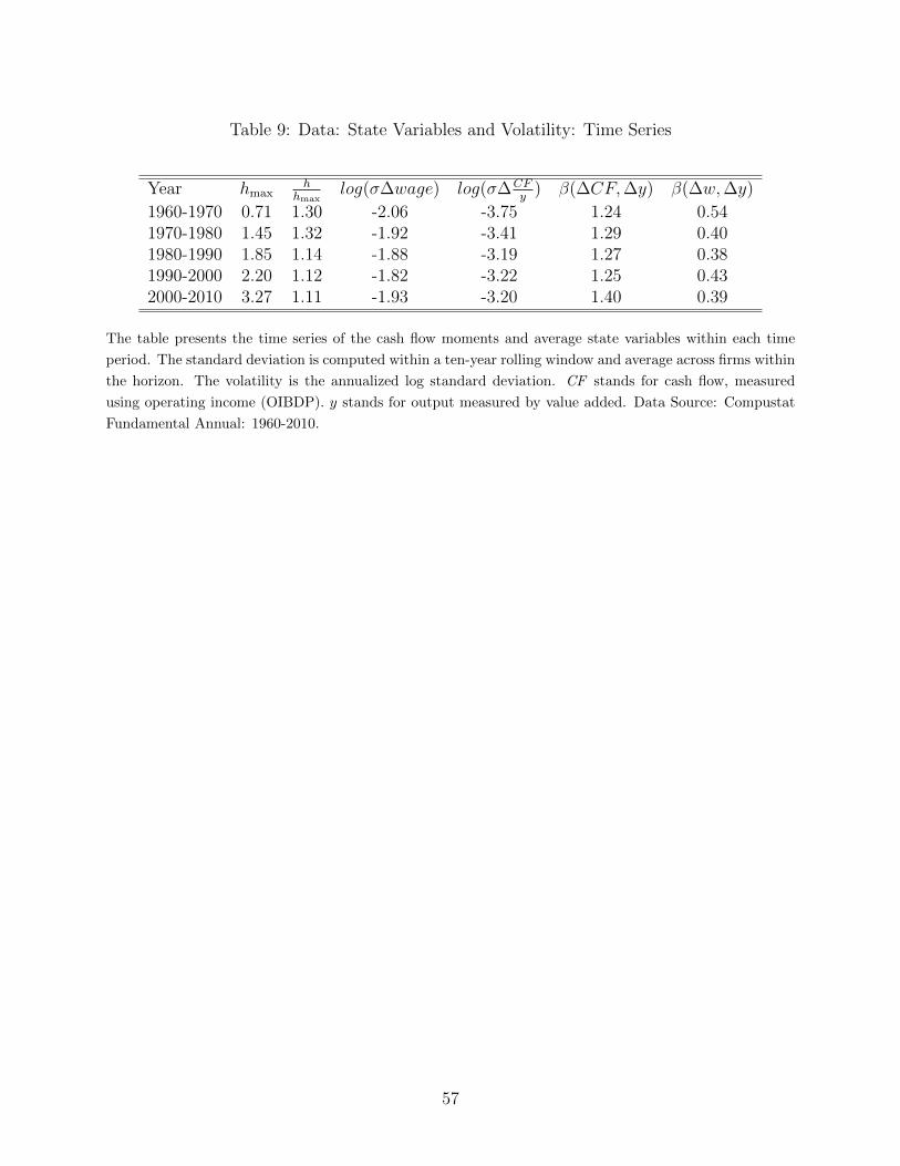
Table 9: Data: State Variables and Volatility: Time Series
Year hmaxh
hmaxlog(σ∆wage) log(σ∆CF
y) β(∆CF,∆y) β(∆w,∆y)
1960-1970 0.71 1.30 -2.06 -3.75 1.24 0.541970-1980 1.45 1.32 -1.92 -3.41 1.29 0.401980-1990 1.85 1.14 -1.88 -3.19 1.27 0.381990-2000 2.20 1.12 -1.82 -3.22 1.25 0.432000-2010 3.27 1.11 -1.93 -3.20 1.40 0.39
The table presents the time series of the cash flow moments and average state variables within each time
period. The standard deviation is computed within a ten-year rolling window and average across firms within
the horizon. The volatility is the annualized log standard deviation. CF stands for cash flow, measured
using operating income (OIBDP). y stands for output measured by value added. Data Source: Compustat
Fundamental Annual: 1960-2010.
57

Table 10: Wage Contract and Firm-Level Human Capital Accumulation History
wage(I) wage(II)(1) (2) (3) (4)
log(hmax,t) 0.363*** 0.628(0.085) (0.940)
log(TFPmax,t) 0.281*** 0.195***(0.030) (0.072)
log(TFPt) -0.089*** -0.119*** 0.016 0.032(0.012) (0.011) (0.046) (0.060)
MB -0.062*** -0.082*** 0.006 -0.033***(0.020) (0.012) (0.011) (0.011)
Market Cap 0.156*** 0.138*** -0.058* 0.004(0.049) (0.028) (0.032) (0.032)
log(Sales) 0.213*** 0.281*** 0.197*** 0.305***(0.031) (0.023) (0.064) (0.035)
Constant 8.463*** 9.417*** 7.537** 9.984***(0.310) (0.104) (3.156) (0.133)
Year FE y y y yFirm FE y y y yN 43,322 106,353 2,913 13,988R-squared 0.062 0.046 0.122 0.136Firm ID 5,034 10,883 433 1,628
This table reports the coefficients of the following regression:
wageit = α+ ηi + λt + β1hmax,it + β2TFPit + ΓXit + εit,
Wage is log average real wage of each firm. TFP is the total factor productivity at the firm level. TFP
is the residual from estimating a log linear Cobb-Douglas production function for each firm and year. The
estimates are provided by Imrohoroglu and Tuzel (2011). log(hmax) is the log maximum firm-level human
capital level before year t. Market Cap is the log of market capitalization, which is equal to total asset +
market value of equity − common equity. log(Sales) is the log deflated net sales. The details of measurement
and construction of all variables are included in Appendix C. Data Source: Compustat Fundamental Annual
1960-2010. Standard errors in parentheses are clustered, *** p < 0.01, ** p < 0.05, * p < 0.1.
58

Table 11: Wage Contract and Firm-Level Human Capital Accumulation History (Value-Weighted)
wage(I) wage(II)(1) (2) (3) (4)
log(hmax,vw,t) 0.367*** 0.088***(0.026) (0.034)
log(TFPmax,vw,t) 0.167*** 0.036(0.022) (0.039)
log(TFPt) -0.085*** -0.130*** -0.010 0.059(0.010) (0.009) (0.052) (0.056)
MB -0.044*** -0.081*** 0.002 -0.031***(0.014) (0.012) (0.012) (0.011)
Market Cap 0.109*** 0.127*** -0.051 -0.002(0.0347) (0.029) (0.036) (0.032)
log(Sales) 0.170*** 0.296*** 0.180*** 0.311***(0.026) (0.023) (0.057) (0.036)
Constant 9.244*** 9.267*** 9.692*** 9.843***(0.205) (0.103) (0.169) (0.138)
Year FE y y y yFirm FE y y y yN 37,952 106,353 2,510 13,988R-squared 0.160 0.043 0.151 0.130Firm ID 4,908 10,883 414 1,628
This table reports the coefficients of the following regression:
wageit = α+ ηi + λt + β1hmax,it + β2TFPit + ΓXit + εit.
Wage is log average real wage of each firm. TFP is the total factor productivity at the firm level. TFP
is the residual from estimating a log linear Cobb-Douglas production function for each firm and year. The
estimates are provided by Imrohoroglu and Tuzel (2011). log(hmax,vw) is the log maximum value-weighted
firm-level human capital level over the past five years. Market Cap is the log of market capitalization, which
is equal to total asset + market value of equity − common equity. log(Sales) is the log deflated net sales.
The details of measurement and construction of all variables are included in Appendix C. Data Source:
Compustat Fundamental Annual 1960-2010. Standard errors in parentheses are clustered, *** p < 0.01, **
p < 0.05, * p < 0.1.
59

Table 12: Wage Contract Sensitivity and Human Capital Investment
∆wage(I) ∆wage(II) ∆wage(I) ∆wage(II)(1) (2) (3) (4)
Dummy 0.056*** 0.014 0.060*** 0.015-0.003 (0.008) (0.003) (0.011)
∆(LP ) 0.209*** 0.275***(0.004) (0.009)
Dummy×∆(LP ) -0.085*** 0.054(0.009) (0.058)
∆(V alue Added) 0.036*** 0.086***(0.004) (0.007)
Dummy×∆(V alue Added) -0.034*** 0.042(0.007) (0.052)
MB -0.007*** -0.003** 0.003*** -0.001(0.001) (0.001) (0.001) (0.002)
Sales 0.048*** 0.026*** 0.069*** 0.041***(0.003) (0.004) (0.003) (0.004)
Market Cap -0.033*** -0.013*** -0.050*** -0.028***(0.003) (0.003) (0.003) (0.004)
Constant -0.581*** -0.042*** -0.654*** -0.049***(0.007) (0.014) (0.008) (0.016)
Year FE y y y yFirm FE y y y yN 146,218 32,226 146,218 32,226R-squared 0.135 0.272 0.017 0.041Firm ID 15,515 3,672 15,515 3,672
This table reports the coefficients of the following regression:
∆wage = α+ ηi + λt + β1D(hmax,it > hmax,it−1) + β2∆y + β3(Dummy ×∆y) + ΓXit + εit.
Wage growth is the difference in the log average real wage of each firm. ∆y is proxied using firm-level labor
productivity growth and firm-level value added growth. Dummy D(hmax,it > hmax,it−1) = 1 if hmax,it >
hmax,it−1. hmax is the log maximum value-weighted firm-level human capital level over the past five years.
Market Cap is the log of market capitalization, which is equal to total asset + market value of equity −common equity. log(Sales) is the log deflated net sales. The details of measurement and construction of
all variables are included in Appendix C. Data Source: Compustat Fundamental Annual 1960-2010. Robust
standard errors in parentheses, *** p < 0.01, ** p < 0.05, * p < 0.1.
60
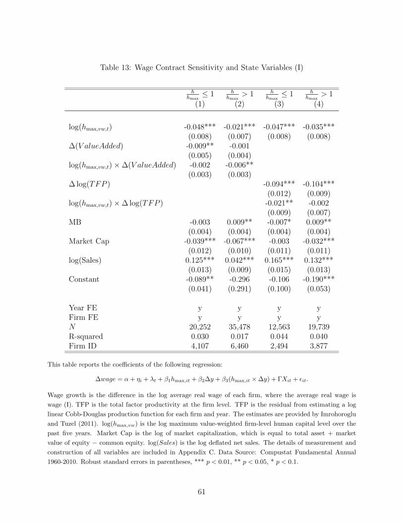
Table 13: Wage Contract Sensitivity and State Variables (I)
hhmax≤ 1 h
hmax> 1 h
hmax≤ 1 h
hmax> 1
(1) (2) (3) (4)
log(hmax,vw,t) -0.048*** -0.021*** -0.047*** -0.035***(0.008) (0.007) (0.008) (0.008)
∆(V alueAdded) -0.009** -0.001(0.005) (0.004)
log(hmax,vw,t)×∆(V alueAdded) -0.002 -0.006**(0.003) (0.003)
∆ log(TFP ) -0.094*** -0.104***(0.012) (0.009)
log(hmax,vw,t)×∆ log(TFP ) -0.021** -0.002(0.009) (0.007)
MB -0.003 0.009** -0.007* 0.009**(0.004) (0.004) (0.004) (0.004)
Market Cap -0.039*** -0.067*** -0.003 -0.032***(0.012) (0.010) (0.011) (0.011)
log(Sales) 0.125*** 0.042*** 0.165*** 0.132***(0.013) (0.009) (0.015) (0.013)
Constant -0.089** -0.296 -0.106 -0.190***(0.041) (0.291) (0.100) (0.053)
Year FE y y y yFirm FE y y y yN 20,252 35,478 12,563 19,739R-squared 0.030 0.017 0.044 0.040Firm ID 4,107 6,460 2,494 3,877
This table reports the coefficients of the following regression:
∆wage = α+ ηi + λt + β1hmax,it + β2∆y + β3(hmax,it ×∆y) + ΓXit + εit.
Wage growth is the difference in the log average real wage of each firm, where the average real wage is
wage (I). TFP is the total factor productivity at the firm level. TFP is the residual from estimating a log
linear Cobb-Douglas production function for each firm and year. The estimates are provided by Imrohoroglu
and Tuzel (2011). log(hmax,vw) is the log maximum value-weighted firm-level human capital level over the
past five years. Market Cap is the log of market capitalization, which is equal to total asset + market
value of equity − common equity. log(Sales) is the log deflated net sales. The details of measurement and
construction of all variables are included in Appendix C. Data Source: Compustat Fundamental Annual
1960-2010. Robust standard errors in parentheses, *** p < 0.01, ** p < 0.05, * p < 0.1.
61

Table 14: Wage Contract Sensitivity and State Variables (II)
hhmax≤ 1 h
hmax> 1 h
hmax≤ 1 h
hmax> 1
(1) (2) (3) (4)
log(hmax,vw,t) 0.048* 0.008 0.055* -0.001(0.026) (0.031) (0.030) (0.026)
∆(V alueAdded) 0.082*** 0.041*(0.031) (0.022)
log(hmax,vw,t) ∗∆(V alueAdded) 0.003 -0.060***(0.025) (0.012)
∆ log(TFP ) 0.079 -0.024(0.067) (0.059)
log(hmax,vw,t)×∆ log(TFP ) -0.003 -0.076***(0.044) (0.025)
MB -0.017* 0.002 -0.005 -0.005(0.010) (0.0093) (0.009) (0.011)
Market Cap -0.002 -0.066*** -0.007 -0.006(0.024) (0.024) (0.027) (0.028)
log(Sales) 0.074 0.069* 0.106 0.189***(0.089) (0.040) (0.071) (0.069)
Constant -0.031 -0.222* -0.168 -0.289*(0.112) (0.116) (0.143) (0.160)
Year FE y y y yFirm FE y y y yN 1,102 2,306 676 1,364R-squared 0.114 0.101 0.132 0.104Firm ID 296 519 155 296
This table reports the coefficients of the following regression:
∆wage = α+ ηi + λt + β1hmax,it + β2∆y + β3(hmax,it ×∆y) + ΓXit + εit.
Wage growth is the difference in the log average real wage of each firm, where the average real wage is
wage (II). TFP is the total factor productivity at the firm level. TFP is the residual from estimating a log
linear Cobb-Douglas production function for each firm and year. The estimates are provided by Imrohoroglu
and Tuzel (2011). log(hmax,vw) is the log maximum value-weighted firm-level human capital level over the
past five years. Market Cap is the log of market capitalization, which is equal to total asset + market
value of equity − common equity. log(Sales) is the log deflated net sales. The details of measurement and
construction of all variables are included in Appendix C. Data Source: Compustat Fundamental Annual
1960-2010. Robust standard errors in parentheses, *** p < 0.01, ** p < 0.05, * p < 0.1.
62

Tab
le15
:V
olat
ilit
yan
dF
irm
-Lev
elH
um
anC
apit
alA
ccum
ula
tion
hhmax≤
1h
hmax>
1h
hmax≤
1h
hmax>
1h
hmax≤
1h
hmax>
1
(1)
(2)
(3)
(4)
(5)
(6)
Dep
enden
tV
aria
ble
sσ
(ret
)σ
(ret
)σ
(∆CF/y
)σ
(∆CF/y
)σ
(∆wageII)
σ(∆wageII)
log(h
max,vw
)1.
891*
**-0
.053
0.37
4***
0.06
9**
-0.0
44*
-0.0
66**
(0.1
49)
(0.0
36)
(0.0
63)
(0.0
36)
(0.0
25)
(0.0
27)
Mar
ket
Cap
-1.7
27**
*-0
.076
0.10
0***
0.07
6***
0.00
1-0
.046
(0.2
28)
(0.0
64)
(0.0
38)
(0.0
24)
(0.0
35)
(0.0
31)
log(S
ales
)0.
533*
**-0
.000
2-0
.088
*-0
.001
-0.1
05**
*-0
.058
**(0
.182
)(0
.047
)(0
.049
)(0
.034
)(0
.026
)(0
.026
)M
B0.
149*
*0.
011
0.02
7*0.
009
0.01
70.
025*
*(0
.074
)(0
.019
)(0
.015
)(0
.009
)(0
.012
)(0
.010
)E
mp
0.73
6***
0.00
9-0
.157
***
0.18
2***
-0.0
55*
-0.0
56*
(0.1
90)
(0.0
51)
(0.0
41)
(0.0
32)
(0.0
29)
(0.0
29)
Con
stan
t-7
.720
***
-2.3
35**
*-3
.696
***
-3.0
33**
*-2
.164
***
-1.3
93**
*(2
.203
)(0
.294
)(0
.213
)(0
.248
)(0
.394
)(0
.282
)
Yea
rF
Ey
yy
yy
yF
irm
FE
yy
yy
yy
N25
,679
34,3
5712
,727
18,0
4816
,253
20,1
70R
-squar
ed0.
080
0.01
30.
331
0.32
80.
052
0.02
7F
irm
ID6,
599
6,19
32,
899
4,03
14,
319
3,62
5
Th
ista
ble
rep
orts
the
coeffi
cien
tsof
the
foll
owin
gre
gre
ssio
n:σ
=α
+η i
+λt+β1hmax,it+
ΓX
it+ε it.σ
(ret
)is
esti
mate
dusi
ng
the
CR
SP
dail
yst
ock
retu
rnw
ith
inea
chea
ran
dan
nu
aliz
eth
evol
atil
ity
esti
mate
sto
ob
tain
an
nu
al
stock
retu
rnvo
lati
lity
.σ
(∆CF/y)
isth
est
an
dard
dev
iati
on
of
cash
flow
grow
th∆
CF y
=CF
t−CF
t−
1
0.5Salest+0.5Salest−
1ov
era
ten
-yea
rro
llin
gw
ind
ow.hmax,vw
isth
elo
gm
axim
um
valu
e-w
eighte
dfi
rm-l
evel
hu
man
cap
ital
leve
l
over
the
pas
tfi
veye
ars
scal
edby
Pro
per
ty,
Pla
nt
an
dE
qu
ipm
ent-
Tota
l(G
ross
).M
ark
etC
ap
isth
elo
gof
mark
etca
pit
ali
zati
on
,w
hic
his
equ
al
toto
tal
asse
t+
mar
ket
valu
eof
equ
ity−
com
mon
equit
y.S
ale
are
log
defl
ate
dn
etsa
le.
Th
ed
etail
sof
mea
sure
men
tan
dco
nst
ruct
ion
of
all
vari
ab
les
are
incl
ud
edin
Ap
pen
dix
C.
Dat
aS
ourc
e:C
omp
ust
at
Fu
nd
am
enta
lA
nnu
al
1960-2
010.
Rob
ust
stan
dard
erro
rsin
pare
nth
eses
,***p<
0.01,
**p<
0.0
5,
*p<
0.1.
63

E Figures
Figure 6: Operating Income/Sales Volatility of β(∆w,∆y) Group
1970 1975 1980 1985 1990 1995 2000 2005 2010−5
−4.5
−4
−3.5
−3
−2.5
Vo
l o
f O
pe
rati
ng
In
co
me
/Sa
les
(1
0−
ye
ar
roll
ing
win
do
w)
β(∆ w,∆ y) <25% quantile
β(∆ w,∆ y) 25%−50% quantile
β(∆ w,∆ y) 50%−75% quantile
β(∆ w,∆ y) >75% quantile
The figure shows the time series of cash flow volatility for different wage-output sensitivity βw,y quantiles.
Cash flow growth is measured using operating income scaled by sales: oibdpt−oibdpt−1
0.5Salest+0.5Salest−1. Volatility is
estimated as the standard deviation of cash flow growth over a ten-year rolling window. Within each βw,y
quantile, firm-level volatility is computed by taking a simple average at each year.
64

Figure 7: Within-Industry Operating Income/Sales Volatility of β(∆w,∆y) Group
(a) Consumer Goods
1965 1970 1975 1980 1985 1990 1995 2000 2005 2010
−5
−4.5
−4
−3.5
Vo
l o
f ∆
(Op
era
tin
g I
nc
om
e/S
ale
s)
Consumer Goods
β(∆ w,∆ y) <25% quantile
β(∆ w,∆ y) 25%−50% quantile
β(∆ w,∆ y) 50%−75% quantile
β(∆ w,∆ y) >75% quantile
(b) Manufacturing
1970 1975 1980 1985 1990 1995 2000 2005 2010−5.5
−5
−4.5
−4
−3.5
−3
−2.5
Vo
l o
f ∆
(Op
era
tin
g I
nc
om
e/S
ale
s)
Manufacturing
β(∆ w,∆ y) <25% quantile
β(∆ w,∆ y) 25%−50% quantile
β(∆ w,∆ y) 50%−75% quantile
β(∆ w,∆ y) >75% quantile
(c) Health Products
1970 1975 1980 1985 1990 1995 2000 2005 2010−6
−5.5
−5
−4.5
−4
−3.5
−3
−2.5
Vo
l o
f ∆
(Op
era
tin
g I
nc
om
e/S
ale
s)
Health Products
β(∆ w,∆ y) <25% quantile
β(∆ w,∆ y) 25%−50% quantile
β(∆ w,∆ y) 50%−75% quantile
β(∆ w,∆ y) >75% quantile
(d) Computer, Information and Technology
1970 1975 1980 1985 1990 1995 2000 2005 2010−4.5
−4
−3.5
−3
−2.5
−2
Vo
l o
f ∆
(Op
era
tin
g I
nc
om
e/S
ale
s)
Computer, Information and Technology−NAICS
β(∆ w,∆ y) <25% quantile
β(∆ w,∆ y) 25%−50% quantile
β(∆ w,∆ y) 50%−75% quantile
β(∆ w,∆ y) >75% quantile
The figure shows the time series of cash flow volatility for different wage-output sensitivity βw,y quantiles
within-industry. Cash flow growth is measured using operating income scaled by sales: oibdpt−oibdpt−1
0.5Salest+0.5Salest−1.
Volatility is estimated as the standard deviation of cash flow growth over a ten-year rolling window. Within
each βw,y quantile, firm-level volatility is computed by taking a simple average at each year.
65
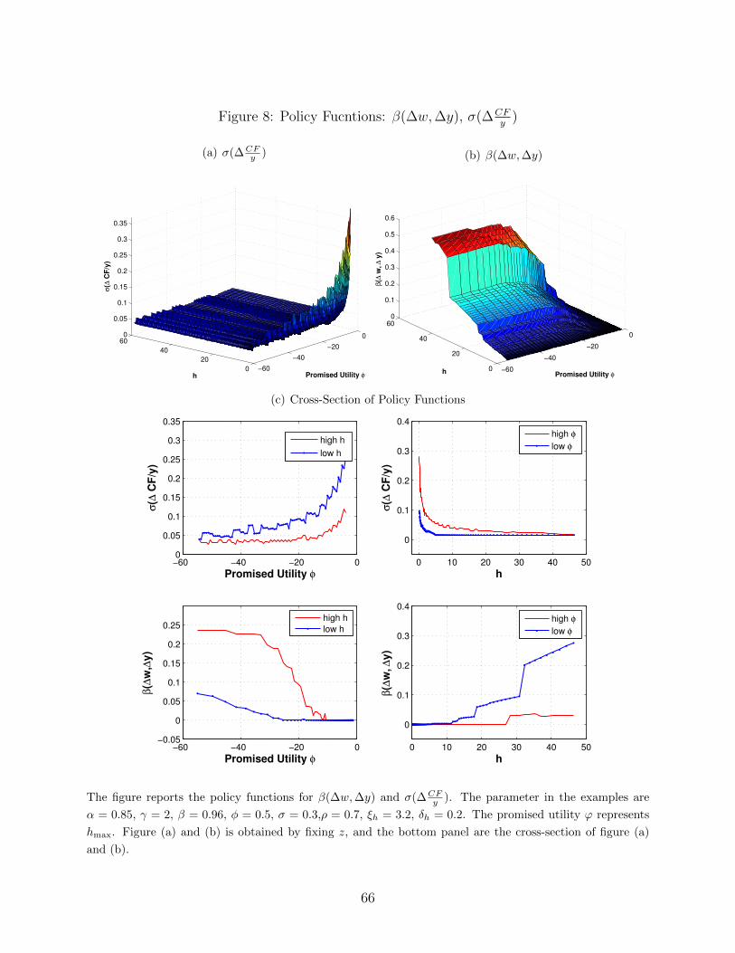
Figure 8: Policy Fucntions: β(∆w,∆y), σ(∆CFy
)
(a) σ(∆CFy )
−60
−40
−20
0
0
20
40
600
0.05
0.1
0.15
0.2
0.25
0.3
0.35
Promised Utility φh
σ(∆
CF
/y)
(b) β(∆w,∆y)
−60
−40
−20
0
0
20
40
60
0
0.1
0.2
0.3
0.4
0.5
0.6
Promised Utility φhβ(∆
w, ∆
y)
(c) Cross-Section of Policy Functions
−60 −40 −20 00
0.05
0.1
0.15
0.2
0.25
0.3
0.35
Promised Utility φ
σ(∆
CF
/y)
high h
low h
0 10 20 30 40 50
0
0.1
0.2
0.3
0.4
h
σ(∆
CF
/y)
high φ
low φ
−60 −40 −20 0−0.05
0
0.05
0.1
0.15
0.2
0.25
Promised Utility φ
β(∆
w,∆
y)
high h
low h
0 10 20 30 40 50
0
0.1
0.2
0.3
0.4
h
β(∆
w, ∆
y)
high φ
low φ
The figure reports the policy functions for β(∆w,∆y) and σ(∆CFy ). The parameter in the examples are
α = 0.85, γ = 2, β = 0.96, φ = 0.5, σ = 0.3,ρ = 0.7, ξh = 3.2, δh = 0.2. The promised utility ϕ represents
hmax. Figure (a) and (b) is obtained by fixing z, and the bottom panel are the cross-section of figure (a)
and (b).
66
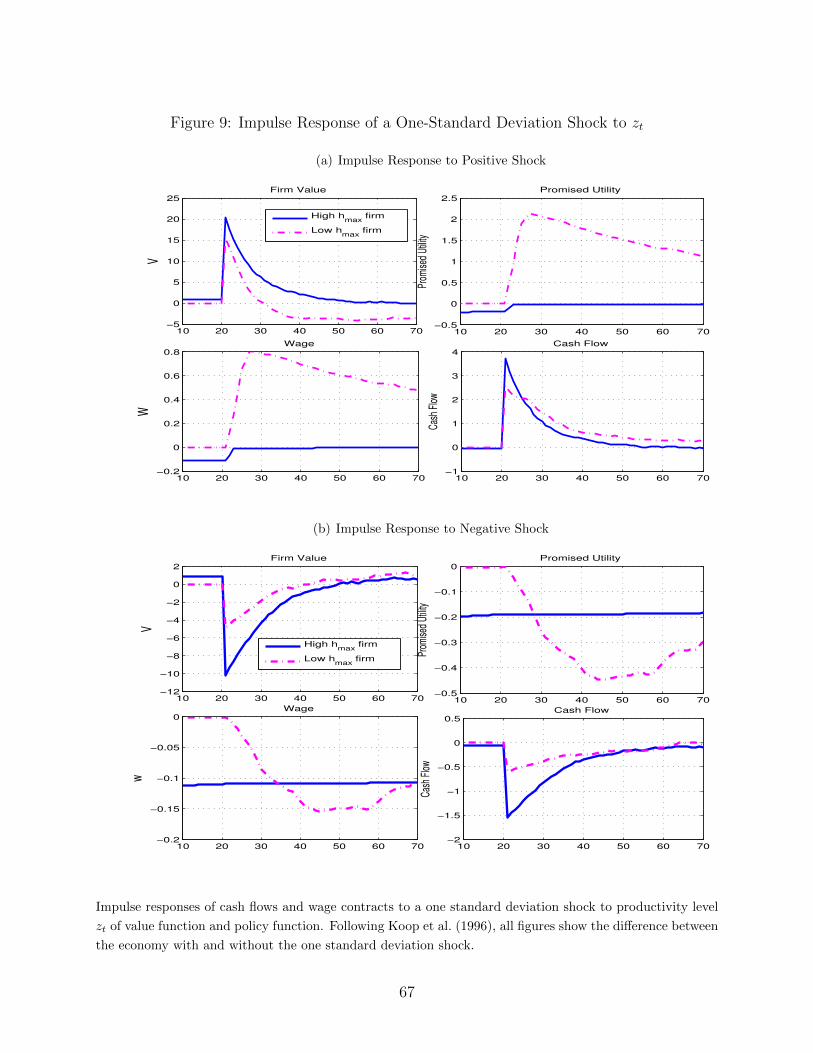
Figure 9: Impulse Response of a One-Standard Deviation Shock to zt
(a) Impulse Response to Positive Shock
10 20 30 40 50 60 70−5
0
5
10
15
20
25
V
Firm Value
High hmax
firm
Low hmax
firm
10 20 30 40 50 60 70−0.5
0
0.5
1
1.5
2
2.5
Prom
ised
Util
ity
Promised Utility
10 20 30 40 50 60 70−0.2
0
0.2
0.4
0.6
0.8
W
Wage
10 20 30 40 50 60 70−1
0
1
2
3
4
Cas
h Fl
ow
Cash Flow
(b) Impulse Response to Negative Shock
10 20 30 40 50 60 70−12
−10
−8
−6
−4
−2
0
2
V
Firm Value
High hmax
firm
Low hmax
firm
10 20 30 40 50 60 70−0.5
−0.4
−0.3
−0.2
−0.1
0Promised Utility
Prom
ised
Util
ity
10 20 30 40 50 60 70−0.2
−0.15
−0.1
−0.05
0Wage
w
10 20 30 40 50 60 70−2
−1.5
−1
−0.5
0
0.5Cash Flow
Cas
h Fl
ow
Impulse responses of cash flows and wage contracts to a one standard deviation shock to productivity level
zt of value function and policy function. Following Koop et al. (1996), all figures show the difference between
the economy with and without the one standard deviation shock.
67
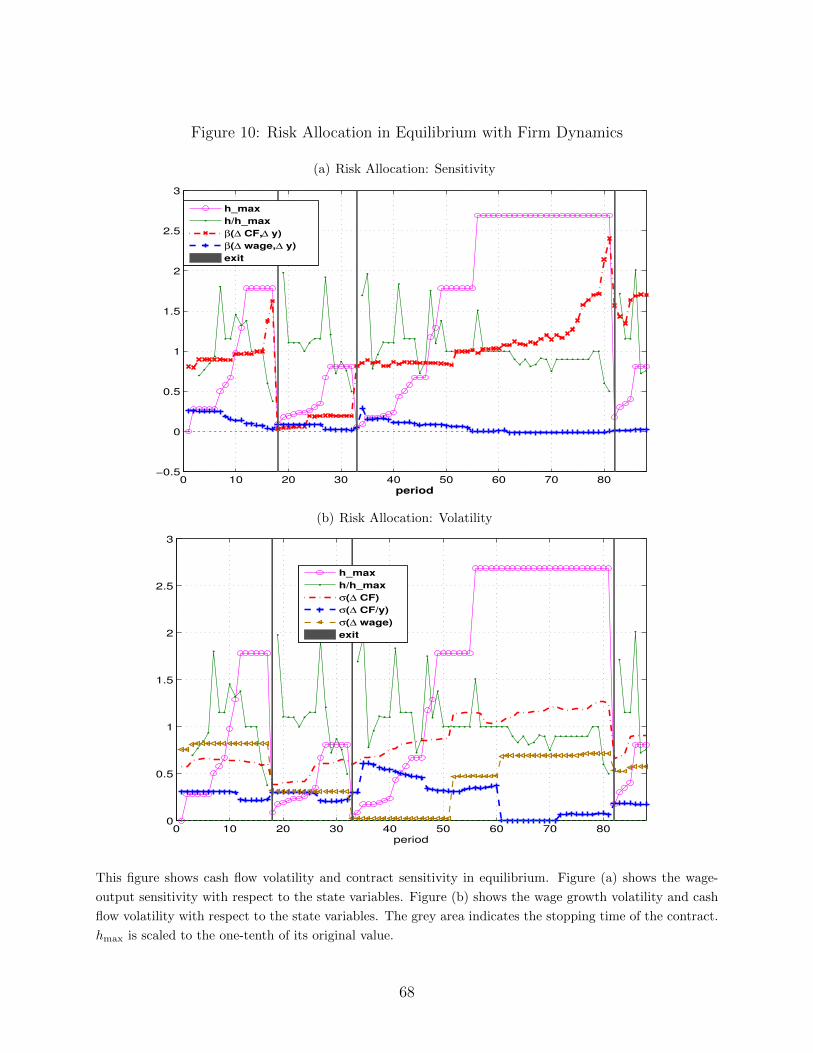
Figure 10: Risk Allocation in Equilibrium with Firm Dynamics
(a) Risk Allocation: Sensitivity
0 10 20 30 40 50 60 70 80−0.5
0
0.5
1
1.5
2
2.5
3
period
h_max
h/h_max
β(∆ CF,∆ y)
β(∆ wage,∆ y)
exit
(b) Risk Allocation: Volatility
0 10 20 30 40 50 60 70 800
0.5
1
1.5
2
2.5
3
period
h_max
h/h_max
σ(∆ CF)
σ(∆ CF/y)
σ(∆ wage)
exit
This figure shows cash flow volatility and contract sensitivity in equilibrium. Figure (a) shows the wage-
output sensitivity with respect to the state variables. Figure (b) shows the wage growth volatility and cash
flow volatility with respect to the state variables. The grey area indicates the stopping time of the contract.
hmax is scaled to the one-tenth of its original value.
68
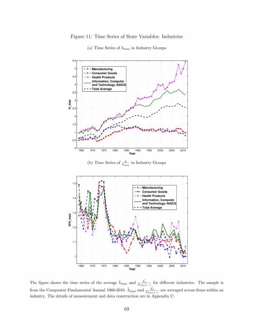
Figure 11: Time Series of State Variables: Industries
(a) Time Series of hmax in Industry Groups
1965 1970 1975 1980 1985 1990 1995 2000 2005 20100
0.5
1
1.5
2
2.5
3
3.5
4
4.5
5
5.5
Year
H_
ma
x
Manufacturing
Consumer Goods
Health Products
Information, Computerand Technology−NAICS
Total Average
(b) Time Series of hhmax
in Industry Groups
1965 1970 1975 1980 1985 1990 1995 2000 2005 2010
1
1.1
1.2
1.3
1.4
1.5
Year
H/H
_m
ax
Manufacturing
Consumer Goods
Health Products
Information, Computerand Technology−NAICS
Total Average
The figure shows the time series of the average hmax and ht
hmax,t−1for different industries. The sample is
from the Compustat Fundamental Annual 1960-2010. hmax and ht
hmax,t−1are averaged across firms within an
industry. The details of measurement and data construction are in Appendix C.
69

Figure 12: Time Series of State Variables in βw,y Groups
(a) Time Series of hmax in βw,y Groups
1965 1970 1975 1980 1985 1990 1995 20000.2
0.4
0.6
0.8
1
1.2
1.4
1.6
1.8
2
Year
H_max,vw
β(∆ w,∆ y) <25% quantile
β(∆ w,∆ y) 25%−50% quantile
β(∆ w,∆ y) 50%−75% quantile
β(∆ w,∆ y) >75% quantile
(b) Time Series of hhmax
in βw,y Groups
1965 1970 1975 1980 1985 1990 1995 2000 20050.9
1
1.1
1.2
1.3
1.4
1.5
1.6
Year
H/H
ma
x,v
w
H/H_max,vw
β(∆ w,∆ y) <25% quantile
β(∆ w,∆ y) 25%−50% quantile
β(∆ w,∆ y) 50%−75% quantile
β(∆ w,∆ y) >75% quantile
The figure shows the time series of hmax and hhmax
for different wage-output sensitivity βw,y quantiles. hmax
is measured as the value-weighted firm-level human capital estimate ht over the past five years. hhmax
is the
ratio between the current year firm-level human capital and the last year maximum human capital level,
hmax,t−1. Within each βw,y quantile, hmax and hhmax
are computed by taking a simple average at each year.
70
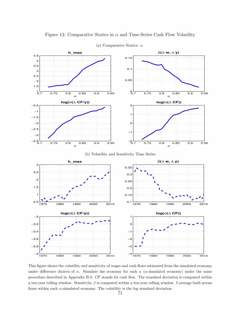
Figure 13: Comparative Statics in α and Time-Series Cash Flow Volatility
(a) Comparative Statics: α
0.7 0.75 0.8 0.85 0.9 0.951
1.5
2
2.5
3
3.5
4
4.5
α
h_max
0.7 0.75 0.8 0.85 0.9 0.950
0.05
0.1
0.15
α
β(∆ w, ∆ y)
0.7 0.75 0.8 0.85 0.9 0.95−3.5
−3
−2.5
−2
−1.5
−1
−0.5
α
log(σ(∆ CF/y))
0.7 0.75 0.8 0.85 0.9 0.95−2
−1
0
1
2
α
log(σ(∆ CF))
(b) Volatility and Sensitivity Time Series
1970 1980 1990 2000 20100.5
1
1.5
2
2.5
3
h_max
1970 1980 1990 2000 20100.1
0.15
0.2
0.25
0.3
0.35
β(∆ w, ∆ y)
1970 1980 1990 2000 2010−4
−3.8
−3.6
−3.4
−3.2
−3
log(σ(∆ CF/y))
1970 1980 1990 2000 2010−4
−3
−2
−1
0
1
log(σ(∆ CF))
This figure shows the volatility and sensitivity of wages and cash flows estimated from the simulated economy
under difference choices of α. Simulate the economy for each α (α-simulated economy) under the same
procedure described in Appendix B.3. CF stands for cash flow. The standard deviation is computed within
a ten-year rolling window. Sensitivity β is computed within a ten-year rolling window. I average both across
firms within each α-simulated economy. The volatility is the log standard deviation.71