white rose environmental effects monitoring design report
TRANSCRIPT

WHITE ROSE
ENVIRONMENTAL EFFECTS MONITORING
DESIGN REPORT
SUBMITTED BY:
HUSKY OIL OPERATIONS LIMITED (AS OPERATOR)
SUITE 801, SCOTIA CENTRE
235 WATER STREET
ST. JOHN’S, NL, AIC 1B6
TEL: (709) 724-3900
FAX: (709) 724-3915
2004

PROJECT NO. NFS09193
FINALWHITE ROSE ENVIRONMENTAL
EFFECTS MONITORING DESIGN REPORT
MAY 2004
Information contained in this report is the Property of Husky Energyand should not be disseminated, used or quoted in part or in whole
without the express written consent of Husky Energy.

PROJECT NO. NFS09193
FINAL
WHITE ROSE ENVIRONMENTALEFFECTS MONITORING DESIGN
REPORT
PREPARED FOR:
HUSKY ENERGYSUITE 801, SCOTIA CENTRE
235 WATER STREETST. JOHN’S, NL A1C 1B6
PREPARED BY:
JACQUES WHITFORD ENVIRONMENT LIMITED607 TORBAY ROAD
ST. JOHN’S, NL A1A 4Y6TEL: (709) 576-1458FAX: (709) 576-2126
MAY 14, 2004

NFS09193 • Husky EEM Design – Report – FINAL • May 14, 2004 Page i© Jacques Whitford 2004
TABLE OF CONTENTS
Page No.
1.0 INTRODUCTION ...................................................................................................................................... 1
1.1 Project Setting and Field Layout ..................................................................................................... 11.2 Project Commitments ...................................................................................................................... 31.3 Environmental Effects Monitoring Objectives ................................................................................ 31.4 Supporting Information for EEM Program Design ......................................................................... 4
1.4.1 White Rose EIS................................................................................................................... 41.4.1.1 Summary of Biological Effect Predictions................................................................... 51.4.1.2 Drill Cuttings and Produced Water Dispersion Modelling .......................................... 5
1.4.2 Baseline Characterization Program .................................................................................... 61.4.3 Stakeholder Consultation.................................................................................................... 6
1.4.3.1 White Rose Environmental Effects Monitoring Advisory Group................................ 61.4.3.2 Consultations with Regulators and Public Information Session .................................. 81.4.3.3 Public Access to EEM Design Document.................................................................... 8
2.0 MONITORING STRATEGY.................................................................................................................... 9
2.1 Marine Resources to be Monitored.................................................................................................. 92.1.1 Sediment Quality .............................................................................................................. 102.1.2 Water Quality ................................................................................................................... 102.1.3 Commercial Fish............................................................................................................... 11
2.2 Sampling Design............................................................................................................................ 122.2.1 Monitoring Hypotheses .................................................................................................... 122.2.2 Sampling Design............................................................................................................... 13
2.2.2.1 Sediment Quality........................................................................................................ 132.2.2.2 Water Quality ............................................................................................................. 192.2.2.3 Commercial Fish ........................................................................................................ 19
3.0 WORK PLAN ........................................................................................................................................... 22
3.1 Sediment Quality ........................................................................................................................... 223.1.1 Sample Collection Method ............................................................................................... 223.1.2 Sample Analysis ............................................................................................................... 23
3.1.2.1 Chemical and Physical Characteristics ...................................................................... 233.1.2.2 Toxicity Testing ......................................................................................................... 253.1.2.3 Benthic Community Status ........................................................................................ 26
3.2 Water Quality................................................................................................................................. 273.3 Commercial Fish............................................................................................................................ 27
3.3.1 Sample Collection Method ............................................................................................... 273.3.2 Sample Analysis ............................................................................................................... 28
3.3.2.1 Body Burden .............................................................................................................. 283.3.2.2 Taste Testing .............................................................................................................. 293.3.2.3 Fish Health ................................................................................................................. 32
4.0 IMPLEMENTATION PLAN .................................................................................................................. 35
4.1 Sampling Platforms ....................................................................................................................... 354.2 Sampling Schedule ........................................................................................................................ 354.3 Documentation............................................................................................................................... 35
4.3.1 Survey Plan....................................................................................................................... 354.3.2 Survey Report ................................................................................................................... 36
5.0 REPORTING AND PROGRAM REVIEW........................................................................................... 37

NFS09193 • Husky EEM Design – Report – FINAL • May 14, 2004 Page ii© Jacques Whitford 2004
5.1 Reporting ....................................................................................................................................... 375.2 Decision Making............................................................................................................................ 375.3 Review and Refinement of Environmental Effects Monitoring Program...................................... 37
6.0 REFERENCES ......................................................................................................................................... 39
6.1 Personal Communications ............................................................................................................. 396.2 Literature Cited.............................................................................................................................. 39
LIST OF APPENDICES
Appendix A Minutes from White Rose Advisory Group Meeting and Table of Concordance of DiscussionsAppendix B Consultation ReportAppendix C Statistical AnalysisAppendix D Statistical Power and RobustnessAppendix E GPS Coordinates of EEM Sediment Stations and Distance to Drill CentresAppendix F Quality Assurance/Quality ControlAppendix G Sediment Chemistry Methods SummariesAppendix H Sediment Particle Size Method SummaryAppendix I Body Burden Methods Summaries
LIST OF FIGURES
Page No.Figure 1.1 Location of the White Rose Oilfield................................................................................................ 1Figure 1.2 White Rose Field Layout ................................................................................................................. 2Figure 1.3 Maximum Extent of Drill Cuttings Dispersion over Life of White Rose Development ................. 7Figure 2.1 Environmental Effects Monitoring Components ............................................................................. 9Figure 2.2 Baseline Station Locations ............................................................................................................ 14Figure 2.3 EEM Program Station Locations and Study and Reference Areas................................................ 16Figure 3.1 Box Corer ...................................................................................................................................... 22Figure 3.2 Allocation of Samples from Cores ................................................................................................ 23Figure 3.3 Questionnaire for Sensory Evaluation by Triangle Test................................................................ 30Figure 3.4 Questionnaire for Sensory Evaluation by Triangle Test................................................................ 31
LIST OF TABLES
Page No.Table 2.1 Table of Concordance Between Baseline and EEM Sediment Station Names.............................. 15Table 2.2 Distances to Nearest Drill Centre for Baseline and EEM Sample Stations ................................... 19Table 3.1 Trace Metal and Hydrocarbon Analysis in Sediment .................................................................... 24Table 3.2 Trace Metal and Hydrocarbon Candidate Parameters ................................................................... 29
Back Pocket
Map of White Rose Final EEM Station Locations

NFS09193 • Husky EEM Design – Report – FINAL • May 14, 2004 Page iii© Jacques Whitford 2004
LIST OF ACRONYMS
ANCOVA Analysis of Co-varianceANOVA Analysis of VarianceAPHA American Public Health AssociationBACI Before-After Control-Impactbbl BarrelCI Control-ImpactC-NOPB Canada-Newfoundland Offshore Petroleum BoardCRM Certified Reference MaterialCTD Conductivity, Temperature and DepthDFO Department of Fisheries and OceansEBM Exaggerated Battlement MethodEEM Environmental Effects MonitoringEIS Environmental Impact StatementEQL Estimated Quantitation LimitEROD enzyme activity referred to as 7-ethoxyresorufin O-deethylaseES Effect SizeFPSO Floating Production, Storage and Offloading (facility)H0 Null (or monitoring) Hypothesiskg Kilogramkm Kilometrekm² Square KilometreL Litrem Metrem3 Cubic MetreMFO Mixed Function Oxygenasemg Milligramml MillilitreMODU Mobile Offshore Drilling UnitNEB National Energy BoardNRC National Research CouncilOGP International Association of Oil and Gas ProducersP Statistical PowerPAH Polycyclic Aromatic HydrocarbonPCA Principal Component AnalysisQA/QC Quality Assurance/Quality ControlRM Repeated MeasureSBM Synthetic-based MudSD Standard DeviationSPMD Semi-permeable Membrane DeviceSQT Sediment Quality TriadTEH Total Extractable HydrocarbonTPH Total Petroleum HydrocarbonTSS Total Suspended SolidsVEC Valued Environmental ComponentW Coefficient of ConcordanceWBM Water-based Mud

NFS09193 • Husky EEM Design – Report – FINAL • May 14, 2004 Page 1© Jacques Whitford 2004
1.0 INTRODUCTION
1.1 Project Setting and Field Layout
Husky Energy, with its joint-venturer Petro-Canada, is in the process of developing the White Roseoilfield on the Grand Banks, offshore Newfoundland. The field is approximately 350 km east southeastof St. John’s, Newfoundland, and 50 km from both the Terra Nova and Hibernia fields (Figure 1.1).
To date, development wells have been drilled at three drill centres: the North (N), Central (C) and South(S) drill centres. Drilling may also occur at two additional centres, one to the north of current centres(NN drill centre) and one to the south of current centres (SS drill centre) (Figure 1.2).
Figure 1.1 Location of the White Rose Oilfield

-------------------------------------------------
-------------------------------------------------
-
5 180 000N
732
500E
720
000E
5 195 500N
NorthDrill Centre724 000.0 E
5 193 900.0 N
WHITE ROSEFPSO
727 725.0 E5 186 025.0 N
CentralDrill Centre725 625.0 E
5 186 005.0 N
2. ALL CO-ORDINATES ARE GIVEN IN METERS AND ARE BASED ONU.T.M. PROJECTION ZONE 22 NAD 83 GRID SYSTEM.
NOTES:
3. ALL HEADINGS ARE RELATIVE TO GRID NORTH.
6. CENTRAL & SOUTHERN FLOWLINE & UMBILICAL SPACING IS 5m ANDNORTHERN SPACING IS 15m.
1. ORIGINAL UNITS ARE IN METERS.
7. MINIMUM CLEARANCE BETWEEN FLOWLINES AND RIG OR FPSO ANCHORS IS 100m.
8. FPSO MOORING SYSTEM GENERAL ARRANGEMENT IS BASED ON MAERSKDRAWING NO. WR-T-91-R-MP-40002-001.
9. 8 POINT MOORING PATTERN BASED ON DRAWING (8 PT MOORING MGT PLANDRAWING 04-JULY-03) RECEIVED FROM CLIENT.
5. CO-ORDINATES INDICATE OVERALL FIELD REFERENCE POINT FOR EACHGLORY HOLE DRILL CENTRE AND THE FPSO.
SouthDrill Centre728 250.0 E
5 184 000.0 N
4. WATER DEPTH IS APPROX. 118-123m. (REF. ENCLOSURE 3 INFUGRO JACQUES GEOSURVEYS INC.'S 2001 WHITE ROSE GEOTECHNICALAND GEOPHYSICAL INVESTIGATION).
NFS
0919
3-E
S-2
0.W
OR
05M
AY0
4 4
:40p
m
WHITE ROSE FIELD LAYOUT
FIGURE 1.2
Legend:
FPSO
Umbilical
Flowline
FPSO Moorings
Anchor for Mobile Drilling Unit
Excavated Sediment Disposal Site
North NorthDrill Centre726 269.5 E
5 196 528.2 N
South SouthDrill Centre728 436.7 E
5 179 122.9 N

NFS09193 • Husky EEM Design – Report – FINAL • May 14, 2004 Page 3© Jacques Whitford 2004
1.2 Project Commitments
Husky Energy committed in its Environmental Impact Statement (EIS) (Part One of the White Rose
Oilfield Comprehensive Study (Husky Oil 2000)) to develop a comprehensive environmental effectsmonitoring (EEM) program for the marine receiving environment. This commitment was integrated intoDecision 2001.01 (C-NOPB 2001) as a condition of project approval. The EEM program would testeffects predictions made in the EIS, detect changes in the marine receiving environment, and determinewhether the changes were caused by the White Rose project.
Also as noted in the C-NOPB’s Decision Report (Condition 38 - Decision 2001.01), Husky Energycommitted, in its application to the C-NOPB, to make the results of its EEM program available tointerested parties and the general public. The C-NOPB also noted that in correspondence to the WhiteRose Public Hearings Commissioner, Husky Energy stated its intent to make both EEM reports andenvironmental compliance monitoring information “publicly available to interested stakeholders in atimely manner”. In fulfilment of Condition 38 noted above, Husky Energy will, in its EnvironmentalProtection Plan, describe how it will make environmentally related information available to the public.
As stated in its Comprehensive Study (Husky Oil 2000), Husky Energy supports the concept of aregional EEM approach, noting that such an approach would have to involve all operators in the area.As such, Husky Energy has had and will continue to have discussions with its fellow operators on thissubject and will report to the C-NOPB on the outcome of those discussions, recognizing the C-NOPB’sinterest in this area.
1.3 Environmental Effects Monitoring Objectives
The EEM program is intended to provide the primary means to determine and quantify project-inducedchange in the surrounding environment. Where such change occurs, the EEM program enables theevaluation of effects and, therefore, assists in identifying the appropriate modifications to, or mitigationof, project activities or discharges. Such operational EEM programs also provide information for the C-NOPB to consider during its periodic reviews of the Offshore Waste Treatment Guideline (NEB et al.2002).
Objectives to be met by the EEM program are:
• confirm the zone of influence of project contaminants;
• test biological effects predictions made in the EIS;
• provide feedback to Husky Energy for project management decisions requiring modification ofoperations practices where/when necessary;
• provide a scientifically defensible synthesis, analysis and interpretation of data;

NFS09193 • Husky EEM Design – Report – FINAL • May 14, 2004 Page 4© Jacques Whitford 2004
• be cost-effective, making optimal use of personnel, technology and equipment; and
• communicate results to the public.
1.4 Supporting Information for EEM Program Design
The design of the White Rose EEM program provided in this document draws on a number of sourcesincluding:
• the White Rose EIS (Husky Oil 2000);
• drill cuttings and produced water dispersion modelling (Hodgins and Hodgins 2000);
• the White Rose baseline characterization program (Husky Oil 2001);
• input from the White Rose Advisory Group (WRAG);
• stakeholder consultations; and
• consultations with regulatory agencies.
1.4.1 White Rose EIS
The White Rose EIS (Husky Oil 2000) made a series of predictions about potential project effects.These predictions were based on whether or not Valued Environmental Components (VECs) interactedwith the project. A VEC-project interaction was considered to be a potential effect if it could change theVEC, or change the prey species or habitats used by the VEC. VECs identified for White Rose included:fish and fish habitat, fisheries, marine birds, marine mammals and sea turtles. The anticipated severity ofeffects on each VEC was ranked on a scale that considered relative magnitude (high, medium, low,negligible), geographic extent (less than 1 km2, 1 to 10 km2, 11 to 100 km2, 1001 to 10,000 km2, greaterthan 10, 000 km2, or unknown), frequency (less than 10 events per year, 11 to 50, 51 to 100, 1001 to200, or greater than 200 events per year, or unknown) and reversibility.
Effects on each VEC were assessed by a discipline expert who considered:
• the location and timing of the interaction;
• drill cuttings and produced water chemical zone of influence modelling exercises for White Rose;
• the literature on similar interactions and associated effects (including the Hibernia (Mobil Oil 19856)and Terra Nova (Petro-Canada 1995) EISs);
• when necessary, consultation with other experts; and
• results of similar effects assessments and especially, monitoring studies done in other areas.

NFS09193 • Husky EEM Design – Report – FINAL • May 14, 2004 Page 5© Jacques Whitford 2004
Only EIS predictions on fish, fish habitat and fisheries are relevant to the EEM program proposed in thisdocument. Husky Energy will monitor effects on marine birds, marine mammals and sea turtles throughvarious other initiatives, including monitoring of occurrence of these species from project platforms andvessels using weather observers trained in these observations and, developing an action plan forrecovering and releasing birds following collisions with project platforms. Details on these initiativeswill be provided elsewhere. This document also only addresses project effects from development andregular operations at White Rose. Monitoring plans in the event of accidental events, including large oilspills, will be developed elsewhere.
In general, development operations at White Rose were expected to have the greatest effects on near-field sediment quality, through release of drill cuttings, while regular operations were expect to have thegreatest effect on water quality, through release of produced water. Effects of other waste streams (e.g.,deck drainage and domestic waste, bilge discharge) on sediment and water quality were consideredsmall relative to effects of drill cuttings and produced water discharge. The anticipated distribution ofdrill cuttings and produced water (Section 1.4.1.2) was therefore central to determination of effects.
1.4.1.1 Summary of Biological Effect Predictions
Effects of drill cuttings on benthos were expected to be mild (low magnitude) within approximately 500m of drill centres but fairly large (low to high magnitude) in the immediate vicinity of drill centres.However, direct effects to fish populations, rather than benthos (on which some fish feed), as a result ofdrill cuttings discharge were expected to be unlikely. Effects resulting from contaminant uptake byindividual fish (including taint) were expected to range from negligible to low in magnitude and belimited to within 500 m from the point of discharge.
Effects of produced water (and other liquid waste streams) on water quality were expected to belocalized near the point of discharge (see Section 1.4.1.2 for the chemical zone of influence of producedwater). Liquid waste streams were not expected to have any effect on sediment quality and benthos andlow magnitude effects on water quality and plankton. Direct effects on adult fish were expected to benegligible.
Further detail on effects and effects assessment can be obtained from the White Rose EIS (Husky Oil2000). For the purpose the EEM program, testable hypotheses that draw on these effects predictions andon drill cuttings and produced water modelling (Section 1.4.1.2) are developed in Section 2.2.1.
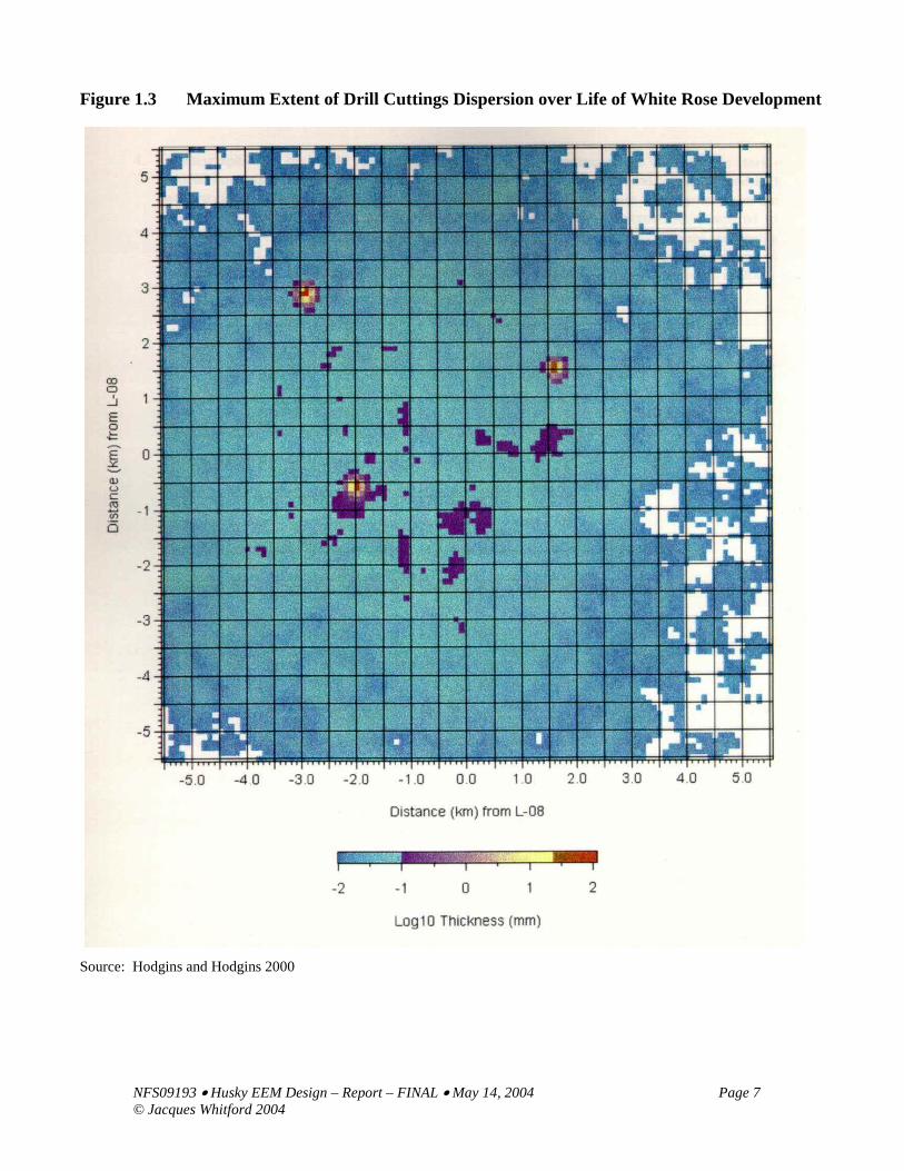
1.4.1.2 Drill Cuttings and Produced Water Dispersion Modelling
Husky Energy modelled the potential dispersion patterns of drill cuttings and produced water (projectdischarges expected to have the greatest effect on environment; see Section 1.4.1) as part of its EIS(Husky Oil 2000). Based on this assessment, the zone of influence of drill cuttings, defined here as the

NFS09193 • Husky EEM Design – Report – FINAL • May 14, 2004 Page 6© Jacques Whitford 2004
zone where project-related physical or chemical alterations might occur, is not expected to extendbeyond approximately 5 km from source (see Figure 1.3 for an example of drill cuttings modellingresults). The zone of influence for produced water is expected to extend to less than 3 km from source.These dispersion pattern results were used to assess the spatial extent of effects in the EIS (see Section1.4.1.1) and to establish the baseline survey grid. Model results will continue to be used as a point ofreference for assessment of EEM results.
1.4.2 Baseline Characterization Program
The White Rose baseline characterization program was designed to provide information on existingconditions at White Rose before development drilling and construction began. Much like the EEMprogram, marine resources targeted for monitoring for this program were selected based on findingsreported in the EIS (see Section 1.4.1.1 and also Section 2.1). The spatial layout of stations aroundWhite Rose for the baseline survey was established given the anticipated distribution of drill cuttings(Section 1.4.1.2). The overall finding from this survey was that the area surrounding White Rose isuncontaminated, notwithstanding prior exploratory drilling and current production operations in theJeanne d’Arc Basin.
1.4.3 Stakeholder Consultation
1.4.3.1 White Rose Environmental Effects Monitoring Advisory Group
Husky Energy committed to organizing an “expert stakeholder group” to help develop the EEM programand potentially provide input into the ongoing interpretation of EEM results. Members of the WRAGincluded (in alphabetical order):
• Leslie Grattan, Consultant;
• Dr. Roger Green, University of Western Ontario;
• Dr. Doug Holdway, University of Ontario Institute of Technology;
• Mary Catherine O’Brien, Lawyer, Manager at Tors Cove Fisheries Ltd.;
• Dr. Paul Snelgrove, Memorial University; and
• Dr. Len Zedel, Memorial University.
NFS09193 • Husky EEM Design – Report – FINAL • May 14, 2004 Page 7© Jacques Whitford 2004
Figure 1.3 Maximum Extent of Drill Cuttings Dispersion over Life of White Rose Development
Source: Hodgins and Hodgins 2000

NFS09193 • Husky EEM Design – Report – FINAL • May 14, 2004 Page 8© Jacques Whitford 2004
The WRAG and the Husky Energy design team met on three occasions (July 22, September 8 andOctober 27, 2003) and also exchanged inform ation throughout the design process. During the firstmeeting (July 22), the WRAG discussed the draft design document which had been previously providedfor review. Most of the recommendations made by the WRAG were made during this meeting andremaining meetings were held either to clarify WRAG position or to bring additional information to theWRAG (including comments from the public and regulators on the EEM design). Minutes from WRAGmeetings, along with a table of concordance summarizing discussion items and Husky Energyresolutions are provided in Appendix A.
1.4.3.2 Consultations with Regulators and Public Information Session
A public information session was held in St. John’s on October 16, 2003. There, Husky Energy providedthe public with a general overview of the EEM program and asked for feedback. A separate meeting washeld with regulatory agencies to discuss the design. The consultation report issuing from these meetingsis provided as Appendix B. This consultation report was also provided to the WRAG (Section 1.4.4.1)for discussion during the October 27th meeting.
1.4.3.3 Public Access to EEM Design Document
This EEM design document will be made available to the public once it is finalized, after regulatoryreview.

NFS09193 • Husky EEM Design – Report – FINAL • May 14, 2004 Page 9© Jacques Whitford 2004
2.0 MONITORING STRATEGY
2.1 Marine Resources to be Monitored
The proposed EEM program is designed around the monitoring of those marine resources targetedduring baseline data collection (and these follow closely from the VECs assessed in the White Rose EIS(Husky Oil 2000)). In addition, given the similarity in production platform and project design (floatingproduction, storage and offloading (FPSO) facility, risers, drill centres) between Terra Nova and WhiteRose (except for scale of project), the White Rose EEM program closely resembles the Terra Nova EEMprogram.
Specifically, data will be collected on sediment quality, water quality and commercial fish species.Proposed EEM components are summarized in Figure 2.1. Details are provided below.
Figure 2.1 Environmental Effects Monitoring Components
Source: modified from Petro-Canada 2002.

NFS09193 • Husky EEM Design – Report – FINAL • May 14, 2004 Page 10© Jacques Whitford 2004
2.1.1 Sediment Quality
Husky Energy made a commitment in the EIS (Husky Oil 2000) to monitor contaminants in sedimentsand their effects on benthic organisms. Regulatory agencies identified oil contamination of sedimentsand effects on benthic organisms as a key indicator of sediment quality and the scientific community hasroutinely monitored sediment quality as part of monitoring programs. Sediments are the ultimate sinkfor persistent chemicals and particulate matter emitted from well development.
Methods to assess the quality of sediments and associated fauna have evolved from basic chemicalanalysis to more exhaustive studies that integrate physical, chemical and biological testing. Threegeneral types of testing are currently used:
• sediment chemical and physical testing;
• sediment toxicity testing; and
• assessment of benthic infaunal community structure.
These tests constitute the Sediment Quality Triad (SQT), an integrative or weight-of-evidence approach(e.g., Long and Chapman 1985; Chapman et al. 1987; Chapman 1992). Assessment of all three SQTcomponents provides more convincing evidence of the spatial extent and magnitude of contaminationthan would any single component.
The SQT approach has been applied to assess the status of sediments near offshore oil platforms in theNorth Sea (Chapman 1992) and in the Gulf of Mexico (Chapman et al. 1991; Chapman and Power 1990;Green and Montagna 1996). The project team has applied the SQT approach in numerous BritishColumbia studies of industrial and municipal discharges and contaminated sites, in the Voisey’s Baymine/mill baseline characterization, and the Hibernia and Terra Nova baseline and EEM programs.Sediment chemical and physical characteristics, toxicity and benthic infaunal community structure weremeasured in the White Rose baseline survey, and will be measured in the White Rose EEM program.
2.1.2 Water Quality
Consistent with WRAG recommendations (see Appendix A), fixed mooring data collection (up to twomoorings) and/or vessel-based sampling will be used to monitor water quality near discharge points andvalidate model predictions on the distribution of produced water. At a minimum, hydrocarbonconcentrations and temperature will be measured in the immediate vicinity of the FPSO. These data willbe supported and interpreted in conjunction with measurements of current velocity and direction derivedfrom Husky Energy’s existing physical environment monitoring program. Hydrocarbon concentrationswill either be measured through use of semi-permeable membrane devices (SPMDs) on fixed mooringsor through vessel-based collections. Husky Energy will also review the feasibility and effectiveness ofusing additional instrumentation installed on existing moorings used for environmental monitoring.

NFS09193 • Husky EEM Design – Report – FINAL • May 14, 2004 Page 11© Jacques Whitford 2004
Moorings data collection (including collection of SPMD data) would be continuous throughout the year.It is anticipated that vessel-based collections would be frequent enough to account for seasonalvariability. A more detailed work plan for water quality data collection will be provided by HuskyEnergy in the autumn of 2004. This revised plan may include water quality parameters additional tothose listed above.
Mooring data collection and/or vessel-based collection will take place from prior to first oil (expected inQ1 2006) to one year after release of produced water (expected in 2007). This should provide sufficientinformation to validate model predictions and confirm the zone of influence of produced water (andother liquid discharges). Once the location of this zone of influence is better defined, Husky Energy willuse the information to design a monitoring program aimed at identifying project effects within the zoneof influence. This design could involve sampling within and outside the zone the influence (Control-Impact design (see Section 2.2.2.3), or sampling at varying distances from source (Attenuation withDistance design (see Section 2.2.2.1) or some other appropriate design. Based on the current schedulefor release of produced water, this new monitoring plan would likely be submitted for review in 2008and implemented in 2008/2009. This plan will take into consideration, among other things, the need andpracticality of monitoring some or all of the parameters subject to measurement in Husky Energy’sproduced water compliance monitoring program pursuant to the Offshore Waste Treatment Guidelines(August 2002).
Collections of data from moorings or vessel platforms, and subsequent collections (as per the revisedmonitoring discussed above) will replace annual collection of water samples and CTD data at sedimentstations, as was done during baseline data collection. This portion of the baseline program was judged tobe of little value by the WRAG and the design team, since it reflects contamination occurringimmediately before sampling, rather than an integrated measure of contamination (as with the sedimentportion of the program).
In addition to the EEM program, Husky Energy is committed to monitoring the quality of its dischargesat source, including produced water, through its compliance monitoring program for developmentdrilling and production to meet the Offshore Waste Treatment Guidelines (NEB et al. 2002).
2.1.3 Commercial Fish
The public and regulators have expressed considerable concern about potential project-related effects onfish, which are, ultimately, the VEC of interest for this EEM program.
On the East Coast of Canada, in the Gulf of Mexico and in the North Sea, researchers have studiedhydrocarbon fate and effects on groundfish and shellfish (Dey et al. 1983; Payne et al. 1983; Neff et al.1985; Berthou et al. 1987; Strickland and Chassan 1989; Paine et al. 1991; 1992). The Hibernia and

NFS09193 • Husky EEM Design – Report – FINAL • May 14, 2004 Page 12© Jacques Whitford 2004
Terra Nova EEM programs include assessments of fish and shellfish tissue chemistry (body burdens),taste and health (physiological, biochemical and histological indicators).
The White Rose EIS (Husky Oil 2000) states that a program to monitor tainting in fish will beimplemented and a DFO position statement (DFO 1997) recommends that a well designed taintingdetection program be initiated around development sites for assurance purposes. The DFO positionstatement also identifies bioaccumulation (i.e., contaminant body burden) as an issue. In the White Rosebaseline survey, American plaice (Hippoglossoides platessoides) were collected for assessment ofmetals and hydrocarbon body burdens, health and taste. Snow crab (Chionoecetes opilio), anothercommercially important species, were also collected for assessment of body burdens and taste. Thesetwo species will continue to be collected and assessed in the EEM program.
2.2 Sampling Design
2.2.1 Monitoring Hypotheses
Monitoring, or null (H0), hypotheses have been established as part of previous EEM programs on theGrand Banks. These hypotheses are implicit to the design and analysis models described in Section 2.2.2(also see Appendices C and D on analysis, and power and robustness, respectively), and were madeexplicit in both the Hibernia and Terra Nova EEM programs to focus and guide interpretation andreporting of results. Null hypotheses differ from EIS effects predictions. They are an analysis andreporting construct established to assess effects predictions. Null hypotheses (H0) will always state “noeffects” even if effects have been predicted as part of the EIS. Therefore, rejection of a null hypothesisdoes not necessarily invalidate EIS predictions, nor should such predictions be considered a“compliance” target in this context.
The following monitoring hypotheses are proposed for the White Rose EEM program:
• Sediment Quality:- H0: There will be no change in SQT variables with distance or direction from project discharge
sources over time.
• Water Quality:- H0: The distribution of produced water from point of discharge, as assessed using moorings data
and/or vessel-based data collection, will not differ from the predicted distribution of producedwater (Note: this null hypothesis will be modified after model validation and review of theproduced water portion of this program).
• Commercial Fish:- H0(1): Project discharges will not result in taint of snow crab and American plaice resources
sampled within the White Rose Study Area, as measured using taste panels.

NFS09193 • Husky EEM Design – Report – FINAL • May 14, 2004 Page 13© Jacques Whitford 2004
- H0(2): Project discharges will not result in adverse effects to fish health within the White RoseStudy Area, as measured using histopathology, haematology and MFO induction.
No hypothesis is developed for American plaice and snow crab body burden, as these tests areconsidered to be supporting tests, providing information to aid in the interpretation of results of othermonitoring variables (taste tests and health).
2.2.2 Sampling Design
2.2.2.1 Sediment Quality
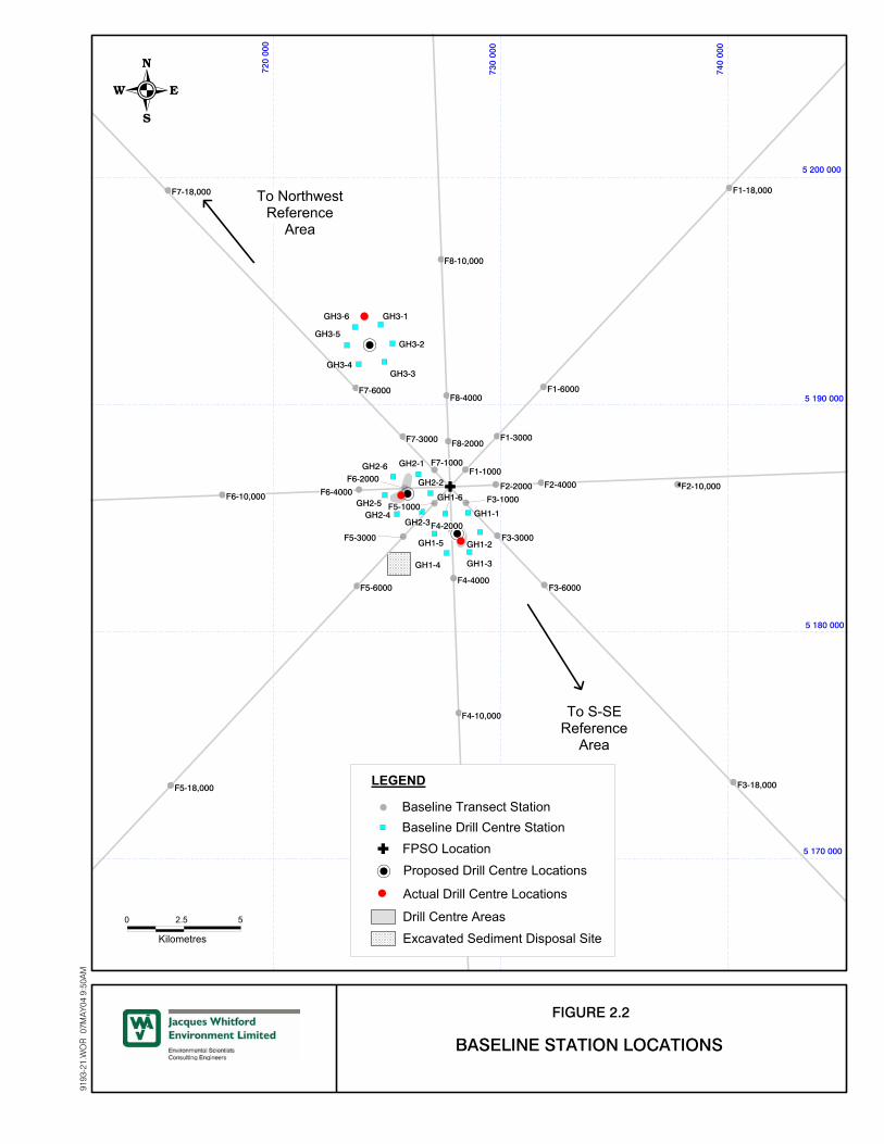
In the baseline survey, three types of sediment quality stations were sampled:
• 28 transect stations, distributed regularly over the Study Area;
• 18 drill centre stations, located within 1 km of the proposed location of the three more central drillcentres; and
• two Reference Areas, one (south-southeast) approximately 35 km from the development, and theother (northwest) approximately 85 km from the development.
The spatial layout of baseline stations is shown in Figure 2.2. For ease of review, station names usedduring baseline will not be used in subsequent programs. Station names during baseline collectioninvolved a series of alpha-numeric codes identifying type of stations and approximate distance to drillcentres. These baseline stations have now been assigned more concise codes. A table of concordancebetween baseline station names and new station names is provided in Table 2.1. Station deletions oradditions noted in Table 2.1 are explained in the text that follows.
The objective of the baseline design was to provide stations representing a range of distances fromsources of contamination (e.g., drill centres). This is a regression or gradient design, suitable for testingfor increases or decreases in SQT variable values (=Y) with distance from source (=X). Regressiondesigns are particularly suitable when there are multiple sources (e.g., drill centres). Distances (and ifneed be, directions) from each source are treated as multiple X variables (see Appendix C for details ondata analysis). If contamination and effects occur, regression designs also provide a broad range of SQTvariable values for assessing correlations among those variables. Replication (=subsampling) withinstations within year is unnecessary. Stations are the appropriate replicates for statistical analyses. Theoptimal strategy is usually to sample more stations as opposed to collecting more subsamples per station(Cuff and Coleman 1979). When the same stations are re-sampled over time, regression designs areRepeated Measures (RM) regression designs.
(
((
(
(
(
(
(
(
(
( (
(
(
(
(
((
(
((
(
(
((
( (
(
-------------------------------------------------
-------------------------------------------------
- GH1-6
GH2-3
GH2-1
GH2-4GH2-5
GH2-6
GH2-2
GH1-5 GH1-2
GH1-1
GH1-4 GH1-3
GH3-3
GH3-1
GH3-2
GH3-4
GH3-6
GH3-5
F5-1000F5-1000F5-1000F5-1000F5-1000F5-1000F5-1000F5-1000F5-1000F3-1000F3-1000F3-1000F3-1000F3-1000F3-1000F3-1000F3-1000F3-1000
F6-4000F6-4000F6-4000F6-4000F6-4000F6-4000F6-4000F6-4000F6-4000
F6-2000F6-2000F6-2000F6-2000F6-2000F6-2000F6-2000F6-2000F6-2000
F5-3000F5-3000F5-3000F5-3000F5-3000F5-3000F5-3000F5-3000F5-3000F4-2000F4-2000F4-2000F4-2000F4-2000F4-2000F4-2000F4-2000F4-2000
F7-1000F7-1000F7-1000F7-1000F7-1000F7-1000F7-1000F7-1000F7-1000
F2-10,000F2-10,000F2-10,000F2-10,000F2-10,000F2-10,000F2-10,000F2-10,000F2-10,000
F8-2000F8-2000F8-2000F8-2000F8-2000F8-2000F8-2000F8-2000F8-2000
F8-4000F8-4000F8-4000F8-4000F8-4000F8-4000F8-4000F8-4000F8-4000
F4-4000F4-4000F4-4000F4-4000F4-4000F4-4000F4-4000F4-4000F4-4000
F2-2000F2-2000F2-2000F2-2000F2-2000F2-2000F2-2000F2-2000F2-2000 F2-4000F2-4000F2-4000F2-4000F2-4000F2-4000F2-4000F2-4000F2-4000
F1-1000F1-1000F1-1000F1-1000F1-1000F1-1000F1-1000F1-1000F1-1000
F1-6000F1-6000F1-6000F1-6000F1-6000F1-6000F1-6000F1-6000F1-6000
F3-6000F3-6000F3-6000F3-6000F3-6000F3-6000F3-6000F3-6000F3-6000F5-6000F5-6000F5-6000F5-6000F5-6000F5-6000F5-6000F5-6000F5-6000
F7-6000F7-6000F7-6000F7-6000F7-6000F7-6000F7-6000F7-6000F7-6000
F8-10,000F8-10,000F8-10,000F8-10,000F8-10,000F8-10,000F8-10,000F8-10,000F8-10,000
F1-18,000F1-18,000F1-18,000F1-18,000F1-18,000F1-18,000F1-18,000F1-18,000F1-18,000
F6-10,000F6-10,000F6-10,000F6-10,000F6-10,000F6-10,000F6-10,000F6-10,000F6-10,000
F5-18,000F5-18,000F5-18,000F5-18,000F5-18,000F5-18,000F5-18,000F5-18,000F5-18,000
F4-10,000F4-10,000F4-10,000F4-10,000F4-10,000F4-10,000F4-10,000F4-10,000F4-10,000
F7-18,000F7-18,000F7-18,000F7-18,000F7-18,000F7-18,000F7-18,000F7-18,000F7-18,000
F3-18,000F3-18,000F3-18,000F3-18,000F3-18,000F3-18,000F3-18,000F3-18,000F3-18,000
F1-3000F1-3000F1-3000F1-3000F1-3000F1-3000F1-3000F1-3000F1-3000F7-3000F7-3000F7-3000F7-3000F7-3000F7-3000F7-3000F7-3000F7-3000
F3-3000F3-3000F3-3000F3-3000F3-3000F3-3000F3-3000F3-3000F3-3000
9193
-21.
WO
R 0
7MA
Y04
9:50
AM
BASELINE STATION LOCATIONS
-------------------------------------------------
Baseline Drill Centre Station
LEGEND
Proposed Drill Centre Locations
Excavated Sediment Disposal Site
Actual Drill Centre Locations
Drill Centre Areas
FIGURE 2.2
720
000
0 2.5
Kilometres
5
5 170 000
5 200 000
5 180 000
5 190 000
740
000
730
000
FPSO Location
To S-SEReference
Area
To NorthwestReference
Area
( Baseline Transect Station
(
(
(
(

NFS09193 • Husky EEM Design – Report – FINAL • May 14, 2004 Page 15© Jacques Whitford 2004
Table 2.1 Table of Concordance Between Baseline and EEM Sediment Station Names
BaselineTransect
Station No.
StationNo. inEEM
Programs
BaselineTransect
Station No.
StationNo. inEEM
Programs
BaselineDrill CentreStation No.
StationNo. inEEM
Programs1
NewBaseline
Drill CentreStation No.²
StationNo. inEEM
ProgramsF1-1,000 1 F5-1,000 16 GH1-1 Deleted SS1 TBDF1-3,000 2 F5-3,000 17 GH1-2 S4 SS2 TBDF1-6,000 3 F5-6,000 18 GH1-3 S1 SS3 TBDF1-18,000 Deleted F5-18,000 Deleted GH1-4 S2 SS4 TBDF2-2,000 5 F6-2,000 20 GH1-5 Deleted SS5 TBDF2-4,000 6 F6-4,000 21 GH1-6 S3 SS6 TBDF2-10,000 7 F6-10,000 22 GH2-1 Deleted NN1 TBDF3-1,000 8 F7-1,000 23 GH2-2 Deleted NN2 TBDF3-3,000 9 F7-3,000 24 GH2-3 C1 NN3 TBDF3-6,000 10 F7-6,000 25 GH2-4 C2 NN4 TBDF3-18,000 11 F7-18,000 26 GH2-5 C3 NN5 TBDF4-2,000 13 F8-2,000 28 GH2-6 C4 NN6 TBDF4-4,000 14 F8-4,000 29 GH3-1 DeletedF4-10,000 15 F8-10,000 31 GH3-2 Deleted
New Transect Station GH3-3 N1Along North Transect 30 GH3-4 Deleted
New Reference Areas3 GH3-5 N2NE ReferenceArea
4 NW ReferenceArea
19 GH3-6 N3
SE ReferenceArea
12 SW ReferenceArea
27
New Near-field Drill Centre Station4 Baseline Reference Areas1
S DrillCentre
S5 N DrillCentre
N4 South-southeast ReferenceArea
Deleted
C DrillCentre
C5 Northwest Reference Area Deleted
1. Baseline Reference Areas and Baseline Drill Centre Station deleted from EEM program (refer to Reference Areasand N, C and S Drill Centre Stations subsections, respectively).
2. Drill Centre Stations added since baseline (refer to NN and SS Drill Centre Stations subsection).3. New Reference Areas were established at 28 km from the FPSO along the NE, SE, SW and NW transects.4. A new station 250 m from drill centre has been added for the N, C and S drill centres. A new 250-m station will beadded for each of the NN and SS drill centres once centre of drill centre is fixed.TBD = To be determined post-2004 EEM program (once centre of drill centre fixed).
Transect Stations
Twenty-six of the 28 transect stations sampled during baseline will be re-sampled in the EEM program.To accommodate the possible expansion of the field to the NN and SS drill centres, four new stationswill be added at 28 km from the centre of the development (Figure 2.3). The constraint used to establishlocation for these stations was that none of them should closer than 20 km from the nearest drill centre.Because of these additions, two 18-km stations, sampled during baseline, will be deleted along thenortheast-southwest axis. However, 18-km stations along the northwest-southeast axis (direction ofprevailing currents) will be retained. One additional sampling station will be added for the EEMprogram: Station 30, near the NN drill centre (see Figure 2.3 and map in back pocket).

-------------------------------------------------
-------------------------------------------------
-
(
(
(
( ((
(
(
(
(
(
(
(
(
(
(
(
(
(
(((
(
(
(
(
(
(
(
(
(
SS5SS5SS5SS5SS5SS5SS5SS5SS5SS4SS4SS4SS4SS4SS4SS4SS4SS4
NN2NN2NN2NN2NN2NN2NN2NN2NN2
NN3NN3NN3NN3NN3NN3NN3NN3NN3
SS6SS6SS6SS6SS6SS6SS6SS6SS6
SS1SS1SS1SS1SS1SS1SS1SS1SS1SS2SS2SS2SS2SS2SS2SS2SS2SS2
SS3SS3SS3SS3SS3SS3SS3SS3SS3
NN1NN1NN1NN1NN1NN1NN1NN1NN1
NN5NN5NN5NN5NN5NN5NN5NN5NN5NN4NN4NN4NN4NN4NN4NN4NN4NN4
262626262626262626
131313131313131313
888888888
202020202020202020
161616161616161616
141414141414141414
171717171717171717
777777777666666666
222222222
555555555
282828282828282828
1
333333333
444444444272727272727272727
252525252525252525
242424242424242424
232323232323232323
212121212121212121
292929292929292929
9
181818181818181818
313131313131313131
303030303030303030
101010101010101010
222222222222222222
151515151515151515
191919191919191919
121212121212121212
111111111111111111
C5C5C5C5C5C5C5C5C5
S3S3S3S3S3S3S3S3S3C1C1C1C1C1C1C1C1C1C2C2C2C2C2C2C2C2C2 S4S4S4S4S4S4S4S4S4
S1S1S1S1S1S1S1S1S1S2S2S2S2S2S2S2S2S2 S5S5S5S5S5S5S5S5S5
C4C4C4C4C4C4C4C4C4
N2N2N2N2N2N2N2N2N2
C3C3C3C3C3C3C3C3C3
N4N4N4N4N4N4N4N4N4
N1N1N1N1N1N1N1N1N1
N3N3N3N3N3N3N3N3N3
200
Mile
Lim
it
150
NFS
1010
7-E
S-2
2.W
OR
7M
AY0
4 1
2:30
PM
EEM PROGRAM STATION LOCATIONSAND STUDY AND REFERENCE AREAS
C Drill Centre Station
LEGEND
Study Area - Commercial Fish Sampling
Drill Centre Locations
NE REFERENCEAREA
720
000
5 170 000
5 200 000
5 180 000
5 190 000
740
000
730
000
FPSO Location
FIGURE 2.3
STUDYAREA
SW REFERENCEAREA
SE REFERENCEAREA
NW REFERENCEAREA
Excavated Sediment Disposal Site
(
(
(
(
(
(
( Transect Station

NFS09193 • Husky EEM Design – Report – FINAL • May 14, 2004 Page 17© Jacques Whitford 2004
Reference Areas
Sediment samples were taken in each of two Reference Areas located approximately 85 km northwestand 35 km south-southeast of the proposed location of the FPSO.
The baseline survey indicated that physical, chemical and biological characteristics of sediments fromthe Northwest Reference Area differed substantially from sediment characteristics of other stations. TheNorthwest Reference Area was an outlier for most baseline analyses, and is unsuitable for future EEMsediment quality monitoring.
Sediment physical and chemical characteristics at the South-southeast Reference Area were reasonablysimilar to those at other stations nearer the development, but the South-southeast Reference Area benthicinfaunal community was clearly different from communities elsewhere.
In the EEM program, the four remote 28-km transect stations will be treated as Reference Areas. Use ofthese 28-km stations as References was recommended by the WRAG based on knowledge of the zoneinfluence of project contaminants in other areas (reported during the Offshore Oil and GasEnvironmental Effects Monitoring Workshop held in Halifax in Spring 2003) and the anticipateddistribution of project contaminants for White Rose (see Section 1.4.1.2).
Drill Centre Stations - North, Central and South Drill Centres
In the baseline survey, there were six drill centre stations located 1 km from the proposed location of theN, C and S drill centres (Figure 2.2). The actual locations of these drill centres, especially the N drillcentre, have shifted since baseline sampling, so these drill centre stations are no longer exactly 1 kmfrom the drill centres (it should be noted that the baseline characterization program in fact assumed thatthe locations of these drill centres would likely move and the program was designed to account for suchmovement). For the purposes of this report, distances for sample stations are distances from thecentroids of the drill centre areas.
The N drill centre will be used for injection of gas and water to maintain pressure at the other two drillcentres, and not for oil extraction. Contamination and effects from that drill centre should be limited.Therefore, baseline stations GH3-1, 3-2 and 3-4 will be deleted from the proposed EEM program. Twobaseline drill centre stations will also be deleted around the C and S drill centres. Baseline stationsGH1-1 and GH1-5 around the S drill centre, and baseline stations GH2-1 and GH2-2 around the C drillcentre, will be deleted. These four stations are further from the drill centres and closer to central transectstations than other drill centre stations. At present, it is not anticipated that the presence of subseaequipment will regularly interfere with sampling these remaining drill centres. The anticipated layout ofsubsea structures is shown in Figure 1.2 (and in the map in the back pocket of this report). Mobile

NFS09193 • Husky EEM Design – Report – FINAL • May 14, 2004 Page 18© Jacques Whitford 2004
offshore drilling unit (MODU) anchors and anchor lines may interfere with sampling, but only at thedrill centre occupied by the MODU, and all stations will be accessible once drilling is complete.
None of the drill centre stations sampled in the baseline survey was within 500 m of the revised or actuallocations of the N, C and S drill centres. The only stations within 500 m of the actual locations weretransect stations F4-2,000 (now Station 13; 470 m from the S drill centre) and F6-2,000 (now Station 20;160 m from the C drill centre). Therefore, one near-field station around each of the N, C and S drillcentre will be added in the EEM program. These stations will be 250 m from the drill centre centroids.The 250 m distance was chosen to maximize exposure to drilling mud contaminants (i.e., provide a“worst-case” scenario), while taking into account the need to ensure safety and project operability.
The locations and sample times for 250-m stations should be regarded as flexible and opportunistic. Aminimum of 42 stations will be re-sampled every EEM year, and regularly re-sampling another threenear-field stations will provide little added value. Instead, the focus should be on extending distanceregressions to low distances and presumably high exposure when possible (see Drill Centre subsection,above, for information on possible interference with sampling when active drilling is occurring).
Drill Centre Stations - NN and SS Drill Centres (Baseline Data Collection)
In addition to the three existing drill centres, Husky Energy may drill in a more northerly drill centre(the NN drill centre) and a more southerly drill centre (the SS drill centre) (see Figure 2.3). Since thelocation of these two new drill centres is not yet fixed, the same approach used during baseline datacollection for the existing drill centres will be used to collect baseline information around these twopotential drill centres. A series of five to six stations located at 1 km from the proposed location of thenew drill centres will be sampled. The assumption here is that if the actual location of these drill centresis no more than 1 km from the proposed location, at least one of the five to six stations sampled shouldbe within 1 km from drill centres. Only five stations are proposed for the NN drill centre because thesixth station would be redundant with Station 31, sampled during baseline. As was done for the N, C andS drill centre stations, those stations that are further away from the actual location of the NN and SS drillcentres, once location has been established, will be deleted from the EEM program. Also, one 250-mstation will be established around each of the new drill centres once locations are fixed.
Summary
Distances from the nearest drill centre for the 48 baseline stations, and for the proposed EEM program(including baseline collections around the NN and SS drill centres) are summarized in Table 2.2.Distance and GPS coordinates for each EEM station are provided in Appendix E. An assessment of thepower and robustness of the EEM design is provided in Appendix D.

NFS09193 • Husky EEM Design – Report – FINAL • May 14, 2004 Page 19© Jacques Whitford 2004
Table 2.2 Distances to Nearest Drill Centre for Baseline and EEM Sample Stations
No. Stations2000 Baseline Program Proposed EEM Program
Distance from NearestDrill centre
(km) Transect andReferenceStations
Drill CentreStations
Total Transect andReferenceStations
Drill CentreStations
Total
≤1 2 8 10 2 21 23>1-2 6 8 14 8 3 11>2-5 12 2 14 12 1 13>5-10 4 0 4 3 0 3>10-20 4 0 4 2 0 2>20 2 0 2 4 0 4Total 30 18 48 28 14 56Note: It is anticipated that two to three stations around each of the NN and SS drill centres will be deleted once the locationof these drill centres is fixed. Assuming that three stations will be deleted around each drill centre, there would be aminimum of 50 stations for the EEM program.
2.2.2.2 Water Quality
Water samples were collected near the surface, at mid-depth, and near the bottom at 13 sediment qualitystations during baseline. CTD data were collected at 25 sediment quality stations. These data will not becollected during the EEM program. This sampling will be replaced with the use of fixed mooring dataand/or more frequent sampling from a vessel platform near points of discharge to determine the zone ofinfluence of produced water (and other liquid waste streams). Once the zone of influence is established,sampling will occur both within and outside this zone. Moorings and/or vessel-based data collection willbegin within the year prior to first oil. Husky Energy will provide a more detailed plan for mooringsand/or vessel-based data collection in the autumn of 2004. A revised water quality monitoring plan willalso be submitted once the zone of influence for produced water is established. This revised plan wouldlikely be submitted in 2008, one year after release of produced water (see Sections 2.1.2 and 3.2.1 fordetails).
2.2.2.3 Commercial Fish
The sampling design for American plaice and snow crab is an ANOVA design (see Appendices C and Dfor details), comparing two or more areas differing in exposure to contamination from the project. Whenonly one Reference Area and one Study Area are sampled, the design is referred to as a Control-Impactor CI design. ANOVA and CI designs are more suitable for large mobile organisms such as fish andshellfish than gradient designs. Areas should be sufficiently separated to ensure that fish or shellfish donot freely move between areas, reducing or eliminating differences in exposure and effects. Based onsuggestions from the WRAG, multiple Reference Areas will be sampled in the White Rose EEMprogram.

NFS09193 • Husky EEM Design – Report – FINAL • May 14, 2004 Page 20© Jacques Whitford 2004
When samples are collected in multiple years, spatial one-way ANOVA designs comparing areasbecome spatial-temporal designs comparing years as well as areas.
Sample Areas
In the baseline survey, American plaice and snow crab were collected by trawl in the Study Area andfrom the Northwest Reference Area. In the EEM program, the Northwest Reference Area will bereplaced by four new Reference Areas, centred on the four 28-km sediment quality stations (refer toFigure 2.3). Based on sediment chemistry, the Northwest Reference Area may not be comparable to theStudy Area. Sampling four References will also provide an estimate of natural large-scale varianceamong Areas, which will be important for assessing the environmental significance of any differencesbetween the References and Study Area (i.e., potential effects) (Appendix C). Finally, it may be difficultto obtain adequate numbers of Reference American plaice or snow crab from a single Area.
Replication Within Areas
In ANOVA designs, there must be replication within Areas. For the White Rose fish and shellfishsurvey, “replicates” are:
• composites of several individuals for body burden analysis;
• taste panelists for taste analysis; and
• individual fish for health assessment.
In a multiple-Reference, the true replicates are arguably Areas, specifically the multiple Reference Areas(Appendix C). However, if there are no significant differences among the Areas, statistical power or theprobability of detecting effects (i.e., differences between Study versus Reference Areas) can beincreased substantially by treating composites or individual fish within Areas as replicates (AppendixD). Furthermore, the taste tests, and specifically the triangle test, are designed to compare samples fromtwo Areas or sources (=pair-wise comparisons), and Reference samples will be pooled for those tests. Itwould be difficult or impossible to make all possible pair-wise comparisons among the four References,and Husky Energy is not aware of any taste study that has attempted to do so.
Sample sizes for body burden analyses should ideally be at least 10 composite samples from the StudyArea, with collection areas distributed relatively evenly between the northern and southern portion of theStudy Area, and at least three composites from each Reference Area (Appendix D). However, if catchesof American plaice and snow crab are low, six composites from the Study Area and two compositesfrom each Reference Area should be regarded as the absolute minima required.

NFS09193 • Husky EEM Design – Report – FINAL • May 14, 2004 Page 21© Jacques Whitford 2004
Similarly, samples sizes for fish health analysis should ideally be at least 60 fish from the Study Area,with collection areas distributed relatively evenly between the northern and southern portion of theStudy Area, and at least 30 fish from each of the Reference Areas (Appendix D) if fish are larger than 25cm (see below). If catch rates are low, 40 fish from the Study Area and 20 fish (25 cm in length) fromeach Reference area should be regarded as the absolute minimum required. More fish may be required iffish size is less than 25 cm, to allow sufficient tissue volume for health and body burden analyses.
Allocation of American plaice tissue in the White Rose EEM program to body burden, taste analysesand health assessment will follow the protocol developed in the Terra Nova EEM program. In the TerraNova program, for American plaice:
• only American plaice >25 cm are retained for analysis, unless catch rates are low;
• trawls are conducted in each area until the required number of American plaice for health analyseshave been collected;
• bottom fillets from each fish are used for body burden analysis, and top fillets are used for tasteanalysis;
• livers are split in half, with one half used for health assessment and one half used for body burdenanalysis (hence the need for American plaice >25 cm); and
• composites for liver and fillet body burden analyses are formed by combining fish tissue from one ormore trawls. All fish in a trawl, rather than a subset of fish, are used for analyses. A minimum of fivefish per replicate is required.
This approach matches composites used for fillet versus liver body burden analyses, and for fillet bodyburden versus taste analysis. The same livers used for body burden analysis are also used for healthassessment, so one could compare health indicator means to body burdens for each body burdencomposite. The same approach can be used for snow crab, which are captured in the same trawls asAmerican plaice. For American plaice, and when sufficient tissue is available, samples from individualfish will be archived for additional body burden analysis if health analyses indicate a potential effect.This should be feasible for fillet samples, but tissue volume will often not be sufficient for individualanalysis on liver.

NFS09193 • Husky EEM Design – Report – FINAL • May 14, 2004 Page 22© Jacques Whitford 2004
3.0 WORK PLAN
3.1 Sediment Quality
3.1.1 Sample Collection Method
The sediment portion of the White Rose EEM program will be conducted in late August/earlySeptember, as was the sediment portion of White Rose baseline characterization program. Sedimentsamples will be collected using a large volume box corer designed to mechanically take an undisturbedsediment sample to a maximum depth of 60 cm over approximately 0.1 m2 of seabed (Figures 3.1).
Positional accuracy for sample collection at each station will be ± 50 m. Three box-core samples will becollected at each station. Sediment samples collected for physical and chemical analysis (refer to Figure2.1), as well as for archive, will be a composite from the top 7.5 cm of all three core sampled (Figure3.2). These will be stored in pre-labelled 250 ml glass jars at -20ºC. Sediment samples collected fortoxicity will be collected from the top 7.5 cm of one core and stored at 4°C in a 4-L pail (amphipodtoxicity) and a Whirl-Pak (bacterial luminescence). Sediment samples for benthic community structureanalysis will be collected from the top 25 cm of two cores and stored in two separate 11-L pails. Thesesamples will be preserved with approximately 1 L of 10 percent buffered formalin.
Figure 3.1 Box Corer

NFS09193 • Husky EEM Design – Report – FINAL • May 14, 2004 Page 23© Jacques Whitford 2004
Figure 3.2 Allocation of Samples from Cores
Source: from Petro-Canada 2002
Sediment chemistry field blanks composed of clean sediment will be collected at 5 percent of sedimentstations. Blank vials will be opened as soon as core samples from selected stations are brought on boardvessel and will remain open until chemistry samples from these stations are processed. Blank vials willthen be sealed and stored with other chemistry samples. Additional Quality Assurance/Quality Control(QA/QC) measures for sample collection and processing are provided in Appendix F (Appendix Fdetails QA/QC for sample collections for all components of the EEM program, as well as QA/QCprocedures for laboratory processing).
3.1.2 Sample Analysis
3.1.2.1 Chemical and Physical Characteristics
Sediment samples will be processed for particle size, hydrocarbons and metals. Specific chemicalcharacteristics to be measured are listed in Table 3.1. Methods summaries for extraction of chemicaldata are provided in Appendix G. Gravel, sand, silt and clay fractions of the sediments will bequantified. Methods summaries for extraction of particle size information are provided in Appendix H.Analysis will be conducted at a CAEAL certified laboratory.

NFS09193 • Husky EEM Design – Report – FINAL • May 14, 2004 Page 24© Jacques Whitford 2004
Table 3.1 Trace Metal and Hydrocarbon Analysis in Sediment
Parameters Method EQL* Units Parameters Method EQL* UnitsHydrocarbons Metals (Total)
Benzene Calculated 0.025 mg/kg Aluminum ICP-MS 10 mg/kgToluene Calculated 0.025 mg/kg Antimony ICP-MS 2 mg/kgEthylbenzene Calculated 0.025 mg/kg Arsenic ICP-MS 2 mg/kgXylenes Calculated 0.05 mg/kg Barium ICP-MS 5 mg/kgC6-C10 (Gas Range) Calculated 2.5 mg/kg Beryllium ICP-MS 5 mg/kg>C10-C21 (Fuel Range) GC/FID 0.25 mg/kg Boron ICP-MS 5 mg/kg>C21-C32 (Lube Range) GC/FID 0.25 mg/kg Cadmium ICP-MS 0.3 mg/kg>C10-C32 (THE) Calculated 0.5 b mg/kg Chromium ICP-MS 2 mg/kgC6-C32 (TPH) Calculated 3.2 mg/kg Cobalt ICP-MS 1 mg/kg
PAHs Copper ICP-MS 2 mg/kg1-Chloronaphthalene GC/FID 0.05 mg/kg Iron ICP-MS 20 mg/kg2-Chloronaphthalene GC/FID 0.05 mg/kg Lead ICP-MS 0.5 mg/kg1-Methylnaphthalene GC/MS 0.05 mg/kg Lithium ICP-MS 2 mg/kg2-Methylnaphthalene GC/MS 0.05 mg/kg Manganese ICP-MS 2 mg/kgAcenaphthene GC/MS 0.05 mg/kg Mercury CVAA 0.01 mg/kgAcenaphthylene GC/MS 0.05 mg/kg Molybdenum ICP-MS 2 mg/kgAnthracene GC/MS 0.05 mg/kg Nickel ICP-MS 2 mg/kgBenz[a]anthracene GC/MS 0.05 mg/kg Selenium ICP-MS 2 mg/kgBenzo[a]pyrene GC/MS 0.05 mg/kg Strontium ICP-MS 5 mg/kgBenzo[b]fluoranthene GC/MS 0.05 mg/kg Thallium ICP-MS 0.1 mg/kgBenzo[ghi]perylene GC/MS 0.05 mg/kg Tin ICP-MS 2 mg/kgBenzo[k]fluoranthene GC/MS 0.05 mg/kg Uranium ICP-MS 0.1 mg/kgChrysene GC/MS 0.05 mg/kg Vanadium ICP-MS 2 mg/kgDibenz[a,h]anthracene GC/MS 0.05 mg/kg Zinc ICP-MS 2 mg/kgFluoranthene GC/MS 0.05 mg/kgFluorene GC/MS 0.05 mg/kgIndeno[1,2,3-cd]pyrene GC/MS 0.05 mg/kg OtherNaphthalene GC/MS 0.05 mg/kg Ammonia (as N) COBAS 0.25 mg/kgPerylene GC/MS 0.05 mg/kg Sulphide SM4500 20 mg/kgPhenanthrene GC/MS 0.05 mg/kg Sulphur LECO 0.03 %(w)Pyrene GC/MS 0.05 mg/kg Moisture Grav. 0.1 %
CarbonTotal Carbon LECO 0.1 g/kgTotal Organic Carbon LECO 0.1 g/kgTotal Inorganic Carbon By Diff 0.1 g/kg* The EQL is the lowest concentration that can be reliably achieved within specified limits of precision and accuracy duringroutine laboratory operating conditions.
Metals and hydrocarbons listed in Table 3.1 are those measured in the Terra Nova EEM program. Thisrevised list of analytes benefits from lessons learned at Terra Nova. For instance, sulphur, sulphide andammonia may affect sediment toxicity (Petro-Canada 2002). Also, 1 and 2-Chloronaphtalenes were notmeasured during the Husky baseline program, but added to the EEM program. With these additions,sediment chemistry analysis for the Terra Nova and White Rose programs are now identical.

NFS09193 • Husky EEM Design – Report – FINAL • May 14, 2004 Page 25© Jacques Whitford 2004
3.1.2.2 Toxicity Testing
Sediment toxicity testing will use standardized and accepted Environment Canada (1998; 2002)procedures. Tests will include:
• amphipod survival; and
• luminescent bacteria assays (Microtox).
Both bioassays will use whole sediment as the test matrix. Tests will include sublethal and lethalendpoints. Tests with lethal endpoints measure survival, in this case amphipod survival, over a definedexposure period. Tests with sublethal endpoints measure physiological functions of the test organism,such as metabolism, fertilization and growth, over a defined exposure period. Bacterial luminescence, inthis case, will be used as a measure of metabolism.
The amphipod survival test will be conducted according to Environment Canada (1998) protocols usingthe marine amphipod Rhepoxynius abronius, if this species is available. In 2003, the population of thesemarine amphipods from Whidbey Island (WA) crashed. Since this is the only North Americancollection site with sediment known to be contaminant-free, the use of an alternate species may berequired if the population has not recovered.
Tests will involve five replicate 1-L test chambers with approximately 2 cm of sediment andapproximately 800 ml of overlying water. Each test container will be set up with 20 test organisms andmaintained for 10 days under appropriate test conditions, after which survival will be recorded. A sixthtest container will be used for water quality monitoring only.
Negative sediment will be tested concurrently, since negative controls provide a baseline response towhich test organisms can be compared. Negative control sediment, known to support a viablepopulation, will be obtained from the collection site for the test organisms. A positive (toxic) control inaqueous solution will be tested for each batch of test organisms received. Positive controls provide ameasure of precision for a particular test and monitor seasonal and batch resistance to a specifictoxicant. Ancillary testing of total ammonia in overlaying water will be conducted by an ammonia ionselective probe and colorimetric determination, respectively.
The bacterial luminescence test will be performed with Vibrio fischeri. This bacterium emits light as aresult of normal metabolic activities. The Microtox (Solid Phase) assay will be conducted according toEnvironment Canada (2002) guidelines. Analysis will be conducted on a Model 500 Photometer with acomputer interface. A geometric series of sediment concentrations will be set up using Azur solid phasediluent. The actual number of concentrations will be dependent on the degree of reduction inbioluminescence observed. Either baseline and/or 18 km stations will be used as “clean” reference

NFS09193 • Husky EEM Design – Report – FINAL • May 14, 2004 Page 26© Jacques Whitford 2004
sediment against which to interpret responses. Reduction of light after 15 minutes will be used tomeasure toxicity.
Microtox analysis for baseline was conducted using the Environment Canada (1992) guideline, whichdiffers from the 2002 guideline. Use of the new Reference Method will create some problems forcomparisons among years, because the highest concentration of sediment to water tested will double,from 98,684 ppm to approximately 167,000 ppm.
All toxicity tests will be initiated within six weeks of sample collection as recommended byEnvironment Canada Guidelines (Environment Canada 1998; 2002).
3.1.2.3 Benthic Community Status
The composition of infaunal communities will be analyzed for two replicate samples collected at eachsediment station. Infaunal community analysis will be used in conjunction with sediment chemistry andtoxicity results to provide an integrated assessment of sediment quality, toxicity and effects on biota.There will be no subsampling for benthic community monitoring. All samples will be kept in 10 percentbuffered formalin until they are sieved (0.5 mm sieve) and sorted at the laboratory. Samples for eachstation will be quantified and identified to the lowest possible taxa. Samples will be sorted separately.
The samples will be processed randomly. For processing, the samples will be poured on a sieve with amesh size of 0.5 mm, then carefully washed using a water pressure low enough so that small or delicateanimals are not damaged. Once the preservatives and fine-grained materials are removed, the animalswill be picked from the remaining sediment. Initially, the washed sample will be placed in an enameltray and the larger animals will be picked out under 2X magnification. Smaller animals will be pickedout under at least 10X magnification. A count of heads will be done when fragments are encountered,and the whole sample will be examined this way. All animals will be preserved in 70 percent alcoholand sieves will be rinsed thoroughly between samples.
Approximately 10 percent of the samples will be retained for re-examination to determine sortingefficiency. This will be recorded on a separate sheet and labelled “sorted debris”. A reference collectionwill be maintained in the laboratory at the time of sorting.
To determine wet weight biomass, all animals will be placed together on paper towels and blotted dry.The material will be weighed in a tiered plastic weighing dish to 0.1-mg accuracy. The volume of graveland shell hash will be recorded for infauna samples.

NFS09193 • Husky EEM Design – Report – FINAL • May 14, 2004 Page 27© Jacques Whitford 2004
3.2 Water Quality
Fixed moorings would be installed reasonably close to the point of discharge within the year prior tofirst oil (see Section 2.1.2). Sensors on fixed moorings would be installed no deeper than 10 m and asclose to surface as feasible. At present, it is anticipated that temperature measurements would becollected every hour at a minimum and every 5 minutes at a maximum. Frequency of measurement willdepend on instrument specification. These instruments would likely be serviced once per month ifSPMDs are used to measure hydrocarbons. On the Norwegian shelf, it was found that optimal residencetime for SPMDs was three to five weeks. After that, the SPMDs became a base for algal growth (A.Melbye, pers. comm.). In the event that data are collected from a vessel platform, samples would againbe collected reasonably close to the point of discharge. A more detailed work plan for water quality datacollection will be provided by Husky Energy in the autumn of 2004. At present, the WRAG and thedesign team have identified water temperature and hydrocarbon accumulation as the most importantparameters to measure. A revised water quality monitoring plan based on results observed during thefirst years of monitoring will also be submitted, likely in 2008 (see Section 2.1.2).
3.3 Commercial Fish
As with the baseline characterization program, the EEM program will focus on American plaice (aspecies common to all three oil and gas operations on the Grand Banks) and snow crab (a commercialspecies common in the White Rose development area).
Samples will be collected in June or July, to match baseline data collection time and assure that adequatesample sizes are collected. Samples will be collected in all areas. However, the presence of subseainfrastructure may interfere with sampling in the immediate vicinity of the development. Every effortwill be made to sample as close to the development as possible, while still meeting safety requirements.
3.3.1 Sample Collection Method
American plaice will be collected in the Study Area (target sample = 60 fish, 10 trawls) and in each offour Reference Areas (target sample = 30 fish, three trawls per area). Samples will be collected with aCampelen trawl (towed at 3 knots for 15 minutes at a series of stations). If catch rates are high,American plaice larger than 25 cm will be selected from the catch at the Study and Reference Areas toallow splitting of livers between body burden analysis and fish health analyses. If catch rates are low,American plaice under 25 cm will be retained for analysis, but a larger number of these small fish maybe needed to allow sufficient tissue volume for analysis (see Section 2.2.2.3 – Replication WithinAreas). Samples will be handled in a consistent manner. All fish retained as samples will show novisible trawl damage or other wounds that could contaminate tissue. Liver and fillets samples will befrozen for taste tests (top fillet only) and body burden (liver and bottom fillet). Liver, gill, blood sampleswill be collected for fish health assessment.

NFS09193 • Husky EEM Design – Report – FINAL • May 14, 2004 Page 28© Jacques Whitford 2004
Approximately 100 kg of snow crab will be collected using the Campelen trawl in the Study Area.Approximately 30 kg of snow crab will also be collected in each of the Reference Areas. Samplesretained for analysis will have no visible trawl damage or other wounds that could contaminate tissue.Legs will be frozen for body burden analysis and taste tests.
Relevant life history and morphometric characteristics will be recorded for both American plaice andsnow crab. Additional measurements on American plaice will include fish length, weight (whole andgutted), sex and maturity stage, liver weight, and gonad weight. Additional measurements for snow crabwill include carapace width, shell condition, sex, chela height (males), and maturity, clutch size and eggstage (females).
All species, other than American plaice or snow crab, caught in trawls will be identified andenumerated.
QA/QC measures applicable to commercial fish collections and sample processing are provided inAppendix F.
3.3.2 Sample Analysis
3.3.2.1 Body Burden
Snow crab and American plaice tissue will be composited as detailed in Section 2.2.2.3 - ReplicationWithin Areas. Composites will be examined for trace metals and a suite of hydrocarbons. ForAmerican plaice and when sufficient tissue is available, tissue from individual fish will be archived foranalysis on individuals in the event that health assessments shows potential effects. The parameters to beanalyzed on composites and individuals (when necessary) are listed in Table 3.2. Methods summariesfor extraction of these data are provided in Appendix I.

NFS09193 • Husky EEM Design – Report – FINAL • May 14, 2004 Page 29© Jacques Whitford 2004
Table 3.2 Trace Metal and Hydrocarbon Candidate Parameters
ParametersMethod EQL Units
ParametersMethod EQL Units
Hydrocarbons Metals>C10-C21 GC/FID 15 mg/kg Aluminum ICP-MS 2.5 mg/kg>C21-C32 GC/FID 15 mg/kg Antimony ICP-MS 0.5 mg/kg>C10-C32 Calculated 45 mg/kg Arsenic ICP-MS 0.5 mg/kg
PAHs Barium ICP-MS 1.5 mg/kg1-Methylnaphthalene GC/MS 0.05 mg/kg Beryllium ICP-MS 1.5 mg/kg2-Methylnaphthalene GC/MS 0.05 mg/kg Boron ICP-MS 1.5 mg/kgAcenaphthene GC/MS 0.05 mg/kg Cadmium ICP-MS 0.08 mg/kgAcenaphthylene GC/MS 0.05 mg/kg Chromium ICP-MS 0.5 mg/kgAnthracene GC/MS 0.05 mg/kg Cobalt ICP-MS 0.2 mg/kgBenz[a]anthracene GC/MS 0.05 mg/kg Copper ICP-MS 0.5 mg/kgBenzo[a]pyrene GC/MS 0.05 mg/kg Iron ICP-MS 5 mg/kgBenzo[b]fluoranthene GC/MS 0.05 mg/kg Lead ICP-MS 0.18 mg/kgBenzo[ghi]perylene GC/MS 0.05 mg/kg Lithium ICP-MS 0.5 mg/kgBenzo[k]fluoranthene GC/MS 0.05 mg/kg Manganese ICP-MS 0.5 mg/kgChrysene GC/MS 0.05 mg/kg Mercury CVAA 0.01 mg/kgDibenz[a,h]anthracene GC/MS 0.05 mg/kg Molybdenum ICP-MS 0.5 mg/kgFluoranthene GC/MS 0.05 mg/kg Nickel ICP-MS 0.5 mg/kgFluorene GC/MS 0.05 mg/kg Selenium ICP-MS 0.5 mg/kgIndeno[1,2,3-cd]pyrene GC/MS 0.05 mg/kg Silver ICP-MS 0.12 mg/kgNaphthalene GC/MS 0.05 mg/kg Strontium ICP-MS 1.5 mg/kgPerylene GC/MS 0.05 mg/kg Thallium ICP-MS 0.02 mg/kgPhenanthrene GC/MS 0.05 mg/kg Tin ICP-MS 0.5 mg/kgPyrene GC/MS 0.05 mg/kg Uranium ICP-MS 0.02 mg/kg
Other Vanadium ICP-MS 0.5 mg/kgPercent Lipids PEI FTC 0.1 % Zinc ICP-MS 0.5 mg/kgMoisture Grav. 0.1 %Crude Fat AOAC922.06 0.5 %(w)Note: Tissue chemistry analyses are identical to those in the Terra Nova Program
3.3.2.2 Taste Testing
American plaice and snow crab samples will be delivered frozen to the testing laboratory for sensoryevaluation, using taste panels and triangle and hedonic scaling test procedures. Frozen samples will bethawed overnight at 4°C and allocated to either the triangle taste or the hedonic scaling test. Tissue fromall Reference Areas will be pooled for comparison with pooled tissue from the Study Areas (the samplevolume for two-way comparisons between the Study Areas and the Reference Areas is excessive andthere are no protocols for a five-way comparison in taste tests). Samples will be rinsed, enclosed inindividual aluminum foil packets (shiny side in), labelled with a pre-determined random three-digitcode, cooked in a convection oven at 175°C for 15 minutes and then served at 35°C. Each panel willinclude 24 untrained panelists who will be provided with score sheets (Figures 3.3 and 3.4) and briefedon the presentation of samples prior to taste tests. Each panelist will be provided with a cup of roomtemperature water for rinsing and a cup for expectorate. Panelists will be instructed not to communicatewith each other while in the panel room and to leave immediately upon completion of the taste tests.

NFS09193 • Husky EEM Design – Report – FINAL • May 14, 2004 Page 30© Jacques Whitford 2004
Figure 3.3 Questionnaire for Sensory Evaluation by Triangle Test

NFS09193 • Husky EEM Design – Report – FINAL • May 14, 2004 Page 31© Jacques Whitford 2004
Figure 3.4 Questionnaire for Sensory Evaluation by Triangle Test
For the triangle test, panelists will be presented with a three-sample set (triangle) of samples and askedto identify the sample that was different from the others. Half of the panelists will receive setscomposed of two samples from Treatment A (Study Areas) and one from Treatment B (ReferenceAreas). The other panelists will receive sets composed of one sample from Treatment A and two fromTreatment B. There will be six possible orders in which the samples were presented to panelists, afterBotta (1994): ABB, AAB, ABA, BAA, BBA, and BAB.

NFS09193 • Husky EEM Design – Report – FINAL • May 14, 2004 Page 32© Jacques Whitford 2004
The rest of the samples will be used for hedonic scaling tests. In this test, one sample from the StudyAreas and one from Reference Areas will be presented to panelists. Panelists will be instructed to ratehow much they liked or disliked each sample on the form provided to them. A nine-point hedonic scalewill be used, with ratings ranging from “like extremely” (9) to “dislike extremely” (1) (see Figure 3.4for full range of ratings).
3.3.2.3 Fish Health
Fish health is a broad term that applies to a number of variables, including examination of tissues forpathological changes (histopathology), blood analysis (haematology), and enzymatic indicators ofexposure to pollutants or stress (e.g., Mixed-Function Oxygenase (MFO)). As much as possible (seeSection 2.2.2.3), fish health analyses will be conducted on the liver, gills and a blood sample of the samefish collected for body burden analysis.
Mixed-Function Oxygenase Induction
Fish liver samples will be thawed slightly on ice and a representative sample (approximately 1 g) will betaken from the same location on each organ. Each liver will be homogenized in four volumes of 50 mMTris buffer (1 g liver to 4 mls 50 mM Tris using ten passes of a glass ten Broek hand Homogenizer). Thehomogenate will be centrifuged at 9,000X g for 10 minutes a 4ºC. The pellet will be discarded and thesupernatant (now known as S9) transferred to Eppendorf microcentrifuge tubes and frozen in triplicate at
-80°C until assayed. In the event that a top fat layer appears, it will be discarded. It is important thatsamples from each site are held under the same storage and assay conditions.
Ethoxy-resorufin o-deethylase (EROD) activity will be assayed fluorometrically as described by Pohland Fouts (1980) and modified by Porter et al. (1989) using a fluorescence spectrophotometer. Thereaction mixture, final volume 1.25 ml, will consist of 53 nmol Tris-Sucrose buffer (50 mM, pH 7.5), 50µl of S9 liver, and 2.25 nmol 7 -ER (150 µM ethoxyresorufin). The reaction mixture will be started bythe addition of 0.16 mg NADPH (1.25 mg/ml). After a 15-minute incubation at 27ºC in a temperature-controlled waterbath, the reaction will be terminated by the addition of a 2.5-ml of ice-cold methanol. Amethanol blank will be used and will contain the same components as the sample tubes, except for theaddition of NADPH. Assay tubes will be vortexed and the protein precipitate removed by centrifugationat 3,600X g for 5 minutes. The fluorescence of resorufin formed in the supernatant will be measured incuvettes (1-cm path length) at 585 nm using an excitation wavelength of 550 nm (slit width of 0.5 mm).The rate of enzyme activity in pmol/min/mg protein will be obtained from the regression of fluorescenceagainst the standard concentrations of resorufin (enzyme activity is linear with time and proteinconcentration).

NFS09193 • Husky EEM Design – Report – FINAL • May 14, 2004 Page 33© Jacques Whitford 2004
All liver samples used for MFO analysis will be treated and processed in the same manner so that anydifference in MFO activity should only be due to sampling area and not affected by processing. Inaddition, when the liver is homogenized and the S9 homogenate prepared, it is frozen in triplicate so thatthere are three identical tubes of homogenate for each liver sample. This is very important becauseEROD activity decreases as the tissue thaws. If this occurs inadvertently, there are two other tubes of thesame sample that can be used as backup.
Histopathology
Both liver and gill samples will be dehydrated in ethanol, cleared in chloroform, and embedded inparaffin wax. Samples will be sectioned at 6 microns and stained with Mayer's haematoxylin and eosin.Additional special stains may be done, if required, to assess various liver lesions. Each sample will beassessed microscopically and a colour photo taken of each section and any lesions observed.
Some of the more notable liver lesions to be looked for in the samples could include:
1. Non-specific necrosis;2. Nuclear pleomorphism;3. Megalocytic hepatosis;4. Eosinophilic foci;5. Basophilic foci;6. Clear cell foci;7. Hepatocellular carcinoma;8. Cholangioma;9. Cholangiofibrosis;10. Increase in mitotic activity; and11. Macrophage aggregates.
According to research carried out by the Environment and Ecosystem Sciences Section (DFO, Science,Oceans and Environment Branch, St. John’s), there are generally six recognized stages used to read gillsections. A colour photograph will be taken of each stage and any tissue abnormalities. It must be keptin mind that the microscopic examination of gill sections is not a quantitative procedure, as all the gilllamellae do not conform to set patterns for each stage. Most times a judgement call is needed;consequently, the skill and experience of the person reading the gills is crucial to the correctinterpretation of the samples. In addition, the presence and number of a variety of cells found in gilltissue will be recorded, including hypertrophic epithelium cells, chloride cells, and mucus cells.

NFS09193 • Husky EEM Design – Report – FINAL • May 14, 2004 Page 34© Jacques Whitford 2004
Similar quality control procedures will be used as with the MFO samples. For both liver and gill tissue, asample will be consistently taken from the same place on each tissue. In addition, serial sections will bemade for each histology sample. This means there will be four sections from the same sample on eachslide. If an abnormality is found in a section, then the other three sections will be checked for the sameabnormality. If it is not found, then the abnormality will be considered an artifact of processing.
Haematology
Blood taken from each fish will be used for haematological assessment. Using the EBM method, allcellular components will be assessed for abnormalities. In terms of haematology analysis, standardroutine procedures will be followed. Because blood cells do not disperse randomly on a slide when ablood smear is made, all sections of the slide will be assessed. The EBM method is a standard procedurethat ensures the entire slide is checked and that cells in one particular area (i.e., the middle or the edges)are not missed.

NFS09193 • Husky EEM Design – Report – FINAL • May 14, 2004 Page 35© Jacques Whitford 2004
4.0 IMPLEMENTATION PLAN
4.1 Sampling Platforms
The sediment survey will be conducted from a suitable supply vessel fitted with a temporary processinglaboratory and supporting infrastructure. The commercial fish survey will be conducted from a DFOcharter vessel.
4.2 Sampling Schedule
The first EEM survey will be conducted in 2004. Surveys will be conducted each year for the first threeyears (i.e., 2004, 2005, 2006). Data collected around the new NN and SS drill centres will be consideredbaseline. Baseline data will also be collected at the four new 28-km Reference areas; these will also beused in future EEM programs. Discussions will be held with the C-NOPB to determine programfrequency for subsequent years. The commercial fish survey will be conducted in late spring/earlysummer, and the sediment survey will be conducted in late summer/early autumn.
A work plan for collection of data aimed at the validation of produced water modelling results will beprovided in the autumn of 2004. Moorings installation, additional instrumentation on existing mooringsand/or vessel-based sampling will be initiated within the year prior to first oil. A revised plan for waterquality monitoring will be provided one year after release of produced water. First oil is expected in Q12006. Release of produced water is expected in 2007.
4.3 Documentation
4.3.1 Survey Plan
Survey plans will be developed prior to the start of the EEM field surveys. Survey plans will providethe overall plan for the field surveys and contain specific information regarding field crew, samplelocations, location coordinates, samples to be collected and priorities for the survey; essentially, thewho, what, where and why of the program. The survey plan is intended as a general overview of theanticipated field operations for use by White Rose operations personnel, the vessel crew and the fieldsurvey team.

NFS09193 • Husky EEM Design – Report – FINAL • May 14, 2004 Page 36© Jacques Whitford 2004
4.3.2 Survey Report
Survey reports will be developed once the sediment and commercial fish field surveys are complete.Survey reports will document the collection of samples by providing a summary of the field operations,including vessel, personnel, mobilization, survey coordinates, a detailed report of the survey activities,demobilization and reporting from the field. Survey reports will also append (as applicable) thesediment sample log, core description log, positioning report, daily field reports, any incident reports(e.g., damaged equipment, survey crew member injury), and tow start and finish coordinates.

NFS09193 • Husky EEM Design – Report – FINAL • May 14, 2004 Page 37© Jacques Whitford 2004
5.0 REPORTING AND PROGRAM REVIEW
5.1 Reporting
Commercial fish and sediment data collected during the EEM program will be compared againstbaseline characterization data (and previous years’ data for each subsequent EEM survey). Whenmoorings data become available, these will be reported as part of the EEM report. The data will bereported in an interpretative document in a plain language format (to the extent possible) to facilitate theusefulness of the EEM program. The report will contain the following basic elements:
• an executive summary that will provide a précis of the report;
• an introduction that will provide an overview of the project description, EEM objectives, and thescope of the EEM program;
• a discussion of the methods used to collect the various types of data;
• the results will provide a comparison of data collected from previous programs and will address theeffectiveness of the program in meeting the EEM objectives;
• the discussion will focus on any changes from previously collected data and a comparison witheffects predictions in the EIS (Husky Oil 2000); and
• the conclusion will highlight key results and identify opportunities for improvement in the program.
5.2 Decision Making
The EEM program is a component of Husky Energy’s environmental management system. The EEMprogram will provide Husky Energy with the information necessary to make project-related decisionsthat may be required in the event that significant measurable effects are detected in the marine receivingenvironment.
5.3 Review and Refinement of Environmental Effects Monitoring Program
The EEM program will be reviewed after each year that data are collected. Husky Energy will continueto consult with the WRAG on its EEM program. Each of the steps in the program will be evaluated and,if necessary, refined to better meet the objectives of the EEM program. At present, it is anticipated thatspecific items for review will include:
• sediment station additions/deletions and sample sizes and locations for commercial fish, particularlyonce drilling is complete;
• specific tests performed on tissue and sediment samples;
• specific analyses performed on data; and
• program frequency after the 2006 field season.

NFS09193 • Husky EEM Design – Report – FINAL • May 14, 2004 Page 38© Jacques Whitford 2004
As the water quality component of the program becomes integrated with the sediment and commercialfish components of the program, specific items of that component will also undergo annual review.
Once finalized, after regulatory review, the EEM interpretative report will be made available in AdobeAcrobat file format on the Husky Energy website.

NFS09193 • Husky EEM Design – Report – FINAL • May 14, 2004 Page 39© Jacques Whitford 2004
6.0 REFERENCES
6.1 Personal Communications
Melbye, A. Research Scientist. SINTEF Applied Chemistry, Trondheim, Norway.
6.2 Literature Cited
Berthou, F., G. Balouet, G. Bodennec, and M. Marchand. 1987. The occurrence of hydrocarbons andhistopathological abnormalities in oysters for seven years following the wreck of the Amoco
Cadiz in Brittany (France). Marine Environmental Research, 23: 103-133.
Botta, J.R. 1994. Sensory evaluation of tainted aquatic resources. Pp. 257-273. In: J.W. Kiceniuk and S.Roy (eds.). Analysis of Contaminants in Edible Aquatic Resources. VCH Publishers, New York,NY.
Chapman, P.M. 1992. Pollution status of North Sea sediments: An international integrative study.Marine Ecology Progress Series, 91: 313-322.
Chapman, P.M., R.N. Dexter, H.A. Anderson and E.A. Power. 1991. Evaluation of effects associatedwith an oil platform, using the Sediment Quality Triad. Environmental Toxicology and
Chemistry, 10: 407-424.
Chapman, P.M., R.N. Dexter and E.R. Long. 1987. Synoptic measures of sediment contamination,toxicity and infaunal community structure (the Sediment Quality Triad) in San Francisco Bay.Marine Ecology Progress Series, 37: 75-96.
Chapman, P.M., M.D. Paine, A.D. Arthur and L.A. Taylor. 1996. A triad study of sediment qualityassociated with major, relatively untreated marine sewage discharge. Marine Pollution Bulletin,32: 47-64.
Chapman, P.M. and E.A. Power. 1990. Sediment Toxicity Evaluation. American Petroleum Institute,No. 4501: 209 pp.
C-NOPB (Canada-Newfoundland Offshore Petroleum Board). 2001. Decision 201.01: Application for
Approval – White Rose Canada-Newfoundland Benefits Plan and White Rose Development Plan.
St. John’s, NL.
Cohen, J. 1988. Statistical Power Analysis for the Behavioral Sciences. 2nd Edition. L. EribaumAssoc., Hillsdale, NJ.

NFS09193 • Husky EEM Design – Report – FINAL • May 14, 2004 Page 40© Jacques Whitford 2004
Cuff, W. and N. Coleman. 1979. Optimal survey designs: Lessons from a stratified random sample ofmacrobenthos. Journal of the Fisheries Research Board of Canada, 36: 351-361.
Dey, A.C., J.W. Kiceniuk, U.P. Williams, R.A. Khan and J.F Payne. 1983. Long term exposure ofmarine fish to crude petroleum. I. Studies on liver lipids and fatty acids in cod (Gadus Morhua)and winter flounder (Pseudopleuronectes americanus). Compendium of Biochemical Physiology,75(1): 93-101.
DFO (Department of Fisheries and Oceans). 1997. Position Statement - Terra Nova Offshore Oil
Development. Submission by the Department of Fisheries and Oceans to the Terra Nova Project
Environmental Assessment Panel. April 1997, St. John’s, NL.
Environment Canada. 1992. Biological Test Method: Toxicity Test using Luminescent Bacteria
(Photobacterium phosphoreum). Report EPS 1/RM/24. Beauregard Printers Ltd. Ottawa, ON.
Environment Canada. 1998. Biological Test Method: Reference Method for Determining Acute
lethality of Sediment to Marine or Estuarine Amphipods. Report EPS 1/RM/35. Ottawa, ON.
Environment Canada. 2002. Biological Test Method: Reference Method for Determining the Toxicity
of Sediment Using Luminescent Bacteria in a Solid-Phase Test. Report EPS 1/RM/42. Ottawa,ON.
Everitt, B.S. 1994. Statistical Methods in Medical Investigations. 2nd Edition. Edward Arnold/Halstead Press, New York, NY.
Green, R.H. 1979. Sampling Design and Statistical Methods for Environmental Biologists. John Wileyand Sons, Toronto, ON.
Green, R.H. 1993. Application of repeated measures design in environmental impact and monitoringstudies. Australian Journal of Ecology, 18: 81-98.
Green, R.H., J.M. Boyd and J.S. Macdonald. 1993. Relating sets of variables in environmental studies:The Sediment Quality Triad as a paradigm. Environmetrics, 44: 439-457.
Green, R.H. and P. Montagna. 1996. Implications for monitoring: study designs and interpretation ofresults. Canadian Journal of Fisheries and Aquatic Sciences, 53: 2,629-2,636.
Hodgins, D.O. and S.L.M. Hodgins. 2000. Modelled Predictions of Well Cuttings Deposition and
Produced Water Dispersion for the Proposed White Rose Development. Part Two Document bySeaconsult Marine Research Ltd. for Husky Oil Operations Limited.

NFS09193 • Husky EEM Design – Report – FINAL • May 14, 2004 Page 41© Jacques Whitford 2004
Husky Oil Operations Limited. 2000. White Rose Oilfield Comprehensive Study - Part One:
Environmental Impact Statement. Submitted to the Canada-Newfoundland Offshore PetroleumBoard, St. John’s, NL.
Husky Oil Operations Limited. 2001. White Rose Baseline Characterization Data Report. Reportprepared by Jacques Whitford Environment Limited for Husky Oil Operations Limited, St.John’s, NL.
Long, E.R. and P.M. Chapman. 1985. A Sediment Quality Triad: Measures of sediment contamination,toxicity and infaunal community composition in Puget Sound. Marine Pollution Bulletin, 16:405-415.
Mobil Oil Canada, Ltd. 1985. Hibernia Development Project - Environmental Impact Statement:
Volumes IIIa and IIIb – Biophysical Assessment. Prepared by Mobil Oil Canada, Ltd. AsOperator, on behalf of the joint venture participants (Gulf Canada Resources Inc., Petro-CanadaInc., Chevron Canada Resources Limited and Columbia Gas Development of Canada Ltd.)involved in the Hibernia Development Project.
NEB, C-NOPB and C-NSOPB (National Energy Board, Canada-Newfoundland Offshore PetroleumBoard and Canada-Nova Scotia Offshore Petroleum Board). 2002. Offshore Waste Treatment
Guidelines.
Neff, J.M., P.D. Boehm and W.E. Haensly. 1985. Petroleum contamination and biochemical alterationsin oysters Crassostrea gigas and plaice Pleuronectes platessa from bays impacted by the Amoco
Cadiz crude oil spill. Marine Environmental Research, 17: 281-283.
Paine, M.D. 1998. Volume II: CANMET/MMSL-INTEMIN. Manual on statistical analysis ofenvironmental data. Prepared for Natural Resources Canada, CANMET, Ottawa, ON., by Paine,Ledge and Associates (PLA), North Vancouver, BC.
Paine, M.D., W.C. Leggett, J.K. McRuer, and K.T. Frank. 1991. Effects of incubation in oiled sedimenton emergence of capelin (Mallotus villosus) larvae. Canadian Journal of Fisheries and Aquatic
Sciences, 48(11): 2,228-2,239.
Paine, M.D., W.C. Leggett, J.K. McRuer, and K.T. Frank. 1992. Effects of Hibernia crude oil oncapelin (Mallotus villosus) embryos and larvae. Marine Environmental Research, 33: 159-187.

NFS09193 • Husky EEM Design – Report – FINAL • May 14, 2004 Page 42© Jacques Whitford 2004
Payne, R., O. Brazier, E.M. Dorsey, J.S. Perkins, V.J. Rowntree and A. Titus. 1983. External features insouthern right whales (Eubalaena australis) and their use in identifying individuals. Pp: 371-445. In: R. Payne (ed.). Communication and Behaviour of Whales. AAAS Sel. Symp. 76.Westview Press, Boulder, CO.
Petro-Canada. 1995. Development Plan Application Terra Nova Development: Environmental Impact
Statement. Report prepared for the Canada-Newfoundland Offshore Petroleum Board, St.John’s, NL.
Petro-Canada. 2002. Terra Nova 2001 Environmental Effects Monitoring Program Year 2. Submittedto the Canada-Newfoundland Offshore Petroleum Board, St. John’s, NL.
Pohl, R.J., and J.R. Fouts. 1980. A rapid method for assaying the metabolism of 7-ethoxyresorufin bymicrosomal subcellular fractions. Analytical Biochemistry, 107: 150-155.
Porter, E.L., J.F. Payne, J. Kiceniuk, L. Fancey and W. Melvin. 1989. Assessment of the potential formixed-function oxygenase enzyme induction in the extrahepatic tissues of cunners duringreproduction. Marine Environmental Research, 28: 117-121.
Sokal, R.R. and F.J. Rohlf. 1981. Biometry. 2nd Edition. W.H. Freeman and Company, New York, NY.
Strickland, R., and D.J. Chasan. 1989. Coastal Washington: A synthesis of information. Washington
State and Offshore Oil and Gas Series, Washington Sea Grant, Seattle, WA.
Tabachnick, B.G. and L.S. Fidell. 1989. Using Multivariate Statistics. 2nd Edition. HarperCollins,New York, NY.
Winer, B.J. 1971. Statistical Principles in Experimental Design. 2nd Edition. McGraw-Hill, New York,NY.

APPENDIX A
Minutes from White Rose Advisory Group Meetingsand Table of Concordance of Discussions

WRAG Meeting Minutes • July 22, 2003 Page 1© Jacques Whitford
White Rose Advisory Group Meeting MinutesJuly 22, 2003
A meeting was held July 22, 2003 with the White Rose Advisory Group (WRAG) to discuss the draftEEM program. In attendance were:
• Dr. Elisabeth DeBlois, Senior Scientist, Jacques Whitford• Leslie Grattan, Environmental Planning and Management Projects, Newfoundland and Labrador
Department of Environment• Dr. Roger Green, Statistician, University of Western Ontario• Dr. Doug Holdway, Ecotoxicologist, University of Ontario Institute of Technology• Mary Catherine O’Brien, Lawyer; Manager at Tors Cove Fisheries Ltd.• Dr. Mike Paine, Statistician, Pain, Ledge and Associates• Dr. Paul Snelgrove, Benthic Ecologist, Memorial University• Dave Taylor, Environmental Coordinator, Husky Energy• Ellen Tracy, Jacques Whitford• Dr. Len Zedel, Memorial University
Dave Taylor, representing Husky Energy, provided an overview of the White Rose Project and ElisabethDeBlois, representing the EEM design team, presented an overview of the draft EEM program.
Issues discussed during the meeting included:
Sediment and Water Quality Components
Use of 18-km stations as controlsThe WRAG felt that the 18-km stations would be adequate Reference Areas and did not supportsampling at either the Northwest Reference Area or the South Southeast Reference Area. There wasdiscussion about adding more distant stations (e.g., 16 km). There was consensus that replication withinstations beyond what is currently proposed (one replicate for benthic invertebrates and no replicates forother variables) was not needed. It was noted that if 18-km stations are used as controls, then a full suiteof samples (sediment, conductivity-temperature-density (CTD) and water samples – but see WaterQuality below) need to collected at these stations. Using all four 18-km stations or selecting two stationsmost comparable to near-field stations was not discussed. The possibility of mapping sediment typesusing geophyphical data collected by Husky Energy was discussed as a possible means of identifyingsuitable Reference Areas.
Near-field Station locationThe WRAG recommended adding stations closer to drill centres. Ideally, new stations would be locatedwithin 500 m (e.g., 250 m and 500 m) from drill centres.
Number of stations overall and powerThe power of the sediment/water sampling grid was discussed. An assessment of the statistical powerand robustness of the proposed design had been provided as appendix material in the draft report andwill be updated if new stations are added.

WRAG Meeting Minutes • July 22, 2003 Page 2© Jacques Whitford
Barium/AluminumThe analysis proposed by Geoff Veinott of DFO was discussed. It was agreed that the method currentlyused is superior to that proposed by DFO if baseline data are available. However, it was felt that usingthis analysis method in addition to the current method would not constitute a large effort. Therefore,provision of these analyses as appendix material was suggested.
Use of isotopes to track the drill cuttings zone of influenceIt was felt that naturally occurring isotopes could be used to track drill cuttings. However, it wasmentioned that hydrocarbons have proved to be very effective tracers in other EEM programs on theGrand Banks.
Water QualityThe usefulness of the water quality monitoring program was questioned. It was generally felt that someground-truthing of predictions made on the distribution of the produced water plume was required. Theinstallation of up to four permanent CTD moorings around the floating production, storage andoffloading (FPSO) facility in order to track currents and better predict the potential location of the plumewas discussed. The availability and utility of current data currently collected for drilling needs to beinvestigated. The use of remote sensing imagery (aerial or satellite) to map the thermal signature(surface only) of the plume was discussed. An adaptive survey strategy for water, based on bestavailable knowledge of plume location, was proposed. It was not clear if the WRAG proposed thesechanges instead of the proposed program or if it felt that additional samples should be collected. Otherthan installation of permanent moorings, the frequency of more targeted water collections was notdiscussed.
Monitoring HypothesisIt was recommended that both the sediment and water monitoring hypotheses be modified to include“effects” of direction as well as distance.
Commercial Fish Component
Use of American plaice as a sentinel speciesGiven the mobility of this species, it was felt that American plaice is more suited to regional monitoringand may not be suitable to assess project-specific effects.
Use of sand lance as a sentinel speciesGiven the information that the WRAG had at hand, there was general agreement that sand lance couldbe a better fish sentinel. It was felt that more information was required on the habits of sand lance toevaluate this species further. It was pointed out that work has been done on Alaskan sand lance; thiscould be used as a starting point.
Usefulness of MFOThe WRAG saw MFO as a useful index of short-term exposure – with the caveat that severalconfounding factors, including reproductive activity and metals contamination, can inhibit MFO. Theuse of a series of health indicators for fish combined with a weight of evidence approach, as is currentlyproposed, was supported.
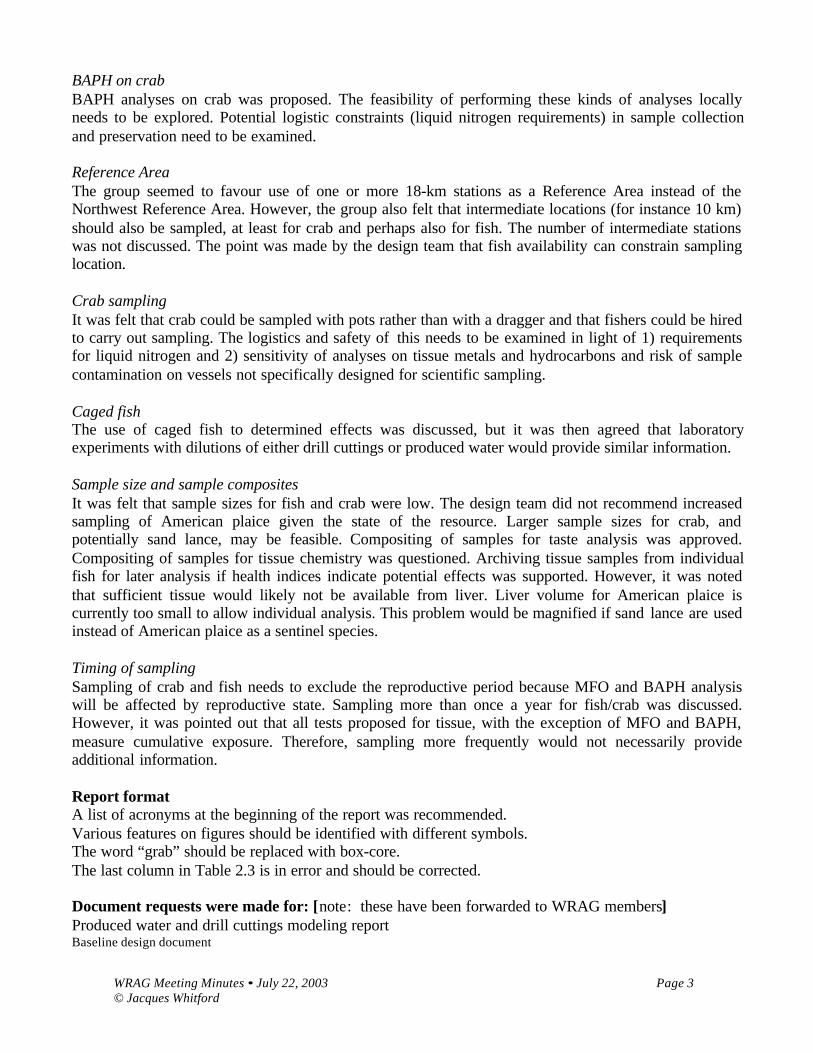
WRAG Meeting Minutes • July 22, 2003 Page 3© Jacques Whitford
BAPH on crabBAPH analyses on crab was proposed. The feasibility of performing these kinds of analyses locallyneeds to be explored. Potential logistic constraints (liquid nitrogen requirements) in sample collectionand preservation need to be examined.
Reference AreaThe group seemed to favour use of one or more 18-km stations as a Reference Area instead of theNorthwest Reference Area. However, the group also felt that intermediate locations (for instance 10 km)should also be sampled, at least for crab and perhaps also for fish. The number of intermediate stationswas not discussed. The point was made by the design team that fish availability can constrain samplinglocation.
Crab samplingIt was felt that crab could be sampled with pots rather than with a dragger and that fishers could be hiredto carry out sampling. The logistics and safety of this needs to be examined in light of 1) requirementsfor liquid nitrogen and 2) sensitivity of analyses on tissue metals and hydrocarbons and risk of samplecontamination on vessels not specifically designed for scientific sampling.
Caged fishThe use of caged fish to determined effects was discussed, but it was then agreed that laboratoryexperiments with dilutions of either drill cuttings or produced water would provide similar information.
Sample size and sample compositesIt was felt that sample sizes for fish and crab were low. The design team did not recommend increasedsampling of American plaice given the state of the resource. Larger sample sizes for crab, andpotentially sand lance, may be feasible. Compositing of samples for taste analysis was approved.Compositing of samples for tissue chemistry was questioned. Archiving tissue samples from individualfish for later analysis if health indices indicate potential effects was supported. However, it was notedthat sufficient tissue would likely not be available from liver. Liver volume for American plaice iscurrently too small to allow individual analysis. This problem would be magnified if sand lance are usedinstead of American plaice as a sentinel species.
Timing of samplingSampling of crab and fish needs to exclude the reproductive period because MFO and BAPH analysiswill be affected by reproductive state. Sampling more than once a year for fish/crab was discussed.However, it was pointed out that all tests proposed for tissue, with the exception of MFO and BAPH,measure cumulative exposure. Therefore, sampling more frequently would not necessarily provideadditional information.
Report formatA list of acronyms at the beginning of the report was recommended.Various features on figures should be identified with different symbols.The word “grab” should be replaced with box-core.The last column in Table 2.3 is in error and should be corrected.
Document requests were made for: [note: these have been forwarded to WRAG members]Produced water and drill cuttings modeling reportBaseline design document

WRAG Meeting Minutes • September 8, 2003 Page 1© Jacques Whitford
White Rose Advisory Group Meeting MinutesSeptember 8, 2003
A second meeting was held September 8, 2002 with the White Rose Advisory Group (WRAG) todiscuss the draft EEM program. In attendance were:
• Dr. Elisabeth DeBlois, Associate Scientist (Oil and Gas), Jacques Whitford• Leslie Grattan, Environmental Planning and Management Projects, Newfoundland and Labrador
Department of Environment• Dr. Roger Green, Statistician, University of Western Ontario• Dr. Doug Holdway, Ecotoxicologist, University of Ontario Institute of Technology• Mary Catherine O’Brien, Lawyer; Manager at Tors Cove Fisheries Ltd.• Dr. Mike Paine, Statistician, Pain, Ledge and Associates• Dr. Paul Snelgrove, Benthic Ecologist, Memorial University• Dave Taylor, Environmental Coordinator, Husky Energy• Ellen Tracy, Jacques Whitford
Issues requiring further clarification since the July 22, 2003 meeting were discussed.
The Advisory agreed that the four 18-km stations should be used as reference stations and that thereference stations used during baseline collections should be dropped. Sampling at reference stationsshould include sediment physical, chemical and biological (benthic invertebrate) characteristics; crab legtissue sampling; American plaice liver and fillet sampling. A water column profile (includingtemperature, salinity, chlorophyll) will also be performed at these, and all, stations.
Use of geophysical data collected by Husky Energy to select reference stations was discussed. MikePaine reported that, from baseline collections, there was variability among the 18-km stations andbetween the 18-km stations and remaining stations. However, this variability was very low and nogreater than what would be expected through distance effects alone (stations that are further apart aremore different than stations closer together).
Installation of one or two permanent moorings within 1 km of the proposed location of the FPSO tomeasure temperature, salinity and chlorophyll was discussed. The advisory group supported thisapproach. The use of semi-permeable membrane devices (SPMDs) to measure hydrocarbonaccumulation was discussed, as we the use of dye tracers. More information will be collected on thesemethods and presented to the Advisory. A discussion will be held with Len Zedel when he returns to getfeedback on benefits of two versus one fixed mooring. The Advisory did not feel that the use of bottomsensors to measure drill cuttings discharge at drill centres was warranted. If sediment hydrocarbon andbarium concentrations do not provide sufficient information on the spread and concentration of drillcuttings (particularly as hydrocarbons degrade), then the use of isotopes could be explored.
The Advisory group agreed that the proposed water sampling program, where water samples arecollected at fixed depths at some sediment stations once a year, or once every two years, should not beexecuted. All were in agreement that this type of sampling provides little information. Instead, theadvisory favoured mapping the produced water plume using available technologies and setting up asampling grid based on the known location of the plume. The advisory recommended that Husky Energyreview its water quality monitoring program a year before release of produced water to afford sufficient

WRAG Meeting Minutes • September 8, 2003 Page 2© Jacques Whitford
time for collection of some baseline data. It was recommended that these fixed moorings be installedone year before release of produced water. Len Zedel will be consulted on fixed moorings.
The use of sand lance instead or in addition to American plaice as a monitoring species was rejected.There is very little known about sand lance. It is classified as a semi-pelagic species that leaves itsburrow at night to feed on plankton. There is no information on horizontal movement of this species. Itmay or may not return to its day location after feeding.
If was felt that the use of additional health indices (metabolites in bile or haemolymph, MFO) oncrab/American plaice was not warranted if contamination could be detected using currentmethodologies. If current methodologies fail to detect contamination, then other indices may beconsidered.
The use of larger samples sizes for crab was discussed. Mike Paine suggested that three to five tissuecomposites per site was sufficient to assess contamination. Roger Green felt that three composites wastoo few. The use of crab pots for sampling crab was rejected because crab can be obtained from trawlscarried out to obtain American plaice. It was proposed that all crab and American plaice in any giventrawl be composited into one sample for metals and hydrocarbon analysis. This would allow someassessment of among trawl variability. Availability of crab and American plaice will determine if this isfeasible.

WRAG Meeting Minutes • October 27, 2003 Page 1© Jacques Whitford
White Rose Advisory Group Meeting MinutesOctober 27, 2003
A third meeting was held October 27, 2003 with the White Rose Advisory Group (WRAG) to discussthe draft EEM program. In attendance were:
• Dr. Elisabeth DeBlois, Associate Scientist (Oil and Gas), Jacques Whitford• Leslie Grattan, Environmental Planning and Management Projects, Newfoundland and Labrador
Department of Environment• Dr. Roger Green, Statistician, University of Western Ontario• Dr. Doug Holdway, Ecotoxicologist, University of Ontario Institute of Technology• Mary Catherine O’Brien, Lawyer; Manager at Tors Cove Fisheries Ltd.• Dr. Mike Paine, Statistician, Paine, Ledge and Associates• Dr. Paul Snelgrove, Benthic Ecologist, Memorial University• Dave Taylor, Environmental Coordinator, Husky Energy• Ellen Tracy, Jacques Whitford• Dr. Len Zedel, Oceanographer, Memorial University
Comments received during consultations with the public and members of the regulatory communitywere discussed, as were any remaining EEM design issues.
Paul Snelgrove recommended that only the first few centimetres (2 cm) of sediment obtained from box-cores be processed for hydrocarbon, metals and particle size analysis. This recommendation wasapproved by the WRAG.
Discussion was held on benthic infauna identification. Infauna are currently identified to the lowesttaxomic level possible and raw data are/will be reported in EEM program reports. There will be clearmention of benthic infauna raw data appendices in both the body of the main report and in Tables ofContents.
Discussion was also held on whether analysis of data for lower taxonomic levels would improve abilityto detect effect. Some WRAG and design team members felt analysis of data for these lower levelswould introduce noise rather than improve analysis. It was agreed that a within-year comparison oflower (in most cases, species) versus higher (in most cases, family) would be of value. There wasdiscussion on potential sources of research funding to undertake such work.
Paul Snelgrove asked for information on how WRAG comments would be integrated into materialsubmitted to regulatory bodies. Dave Taylor responded that meeting minutes and resolutions would besubmitted as part of the EEM design document.
Minor statistical issues were discussed by Mike Paine, Paul Snelgrove and Roger Green. Of these, onlyone follow up issue emerged. Roger Green is to supply Mike Paine with references on use of root-roottransform in MDS. However, given that the analysis is NMDS rather than MDS, it is not clear that thisfollow-up item is still relevant.
Given the MDS/NMDS confusion, it was again recommeded that any acronyms used in EEM design andreport documents be clearly defined at the front of documents.

WRAG Meeting Minutes • October 27, 2003 Page 2© Jacques Whitford
Comments received from the public and the regulatory community were then discussed.
A general discussion was held on effects of seismic, vessels and development drilling noise on seabirdsand marine mammals. Dave Taylor provided some information on Husky Energy commitments withrespect to these issues. However, Elisabeth DeBlois pointed out that noise effects on seabirds andmarine mammals, as well as effects monitoring requirements in the event of an accidental event wereissues that Husky Energy deals with outside of a standard development drilling and operational EEMprogram. It was recognized by all that these issues are of concern to the public.
Regulator comments on station location were discussed. It was agreed that three new sediment stationslocated 250 to 300 m from Glory Holes (one around each Glory Hole) should be added. Dave Taylorstated that dredge spoils were dumped immediately outside Glory Holes for two of the three GloryHoles. It was recommended that stations be located outside the immediate influence of Glory Holes.Some clarification from the WRAG is required on weather this means “off” dredge spoils. Safetyconstraints were acknowledged and it was recognized that these stations would not necessarily beaccessible during each EEM year. It was recommended that these stations be sampled as often aspossible.
Discussion was held on sampling the dredge spoil pile from the central Glory Hole (located some kms tothe South). Dave Taylor stated that some clarification from DFO was required before such samplingwould be undertaken. The WRAG also felt that the stations already located in the immediate vicinity ofthese dredge spoils might provide some indication of dredge spoil effects.
The water quality monitoring program was discussed at length. It was recommended that two mooringsbe placed as close as possible to the point of discharge for produced water one year before release ofproduced water. Instruments to be installed on these moorings would included CTDs and SPMDs.Additional instrumentation could include a fluorometer for oil detection (if instrument sensitivity issufficient) and “some instrument” to measure concentration of radioactive tracers. Elisabeth DeBloiswill check on the fluorometer sensitivity. Dave Taylor will check on radioactive tracers andinstrumentation for these types of measurement. Dave Taylor will also discuss use of additional sensorswith Ken Lee at the Department of Fisheries and Oceans. It was agreed that data from these mooringswould be supplemented by Husky Energy measurements of current velocity/direction. It wasrecommended that sensors be located as close to the surface as possible and no deeper than 10 m.
With respect to measurement frequency, it was recommended that measurements be collected at leastevery hour but ideally every five minutes. It was also recommended that the instruments be services fourtimes per year and that four set of sensors be purchased. Sensors would be “swapped” at each servicing.
Measurement of other variables such as chlorophyll a and phytoplankton community composition wasdiscussed. However, it was stated that the objective of collecting this mooring data was to verifyproduced water modelling predictions and that these other measurements would not offer substantialimprovement over what was proposed above.
Design options for the commercial fish survey were also discussed at length. More elaborate poweranalyses were discussed. Mike Paine specified that this exercise would be of little value withoutspecification of effects size to be detected. Various concepts and exercises were discussed, includingassessment of Maximum Acceptable Effects Levels (MAEL) for each EEM variable and settingalpha=beta in an assessment of relative power. The difference between statistical significance and

WRAG Meeting Minutes • October 27, 2003 Page 3© Jacques Whitford
biological significance was discussed. A concensus was eventually reached: it was recognized that theuse of four Reference Areas instead of one is an improvement over other program; that other programshave sufficient power to detect small statistical differences and that these small differences have not hadbiological relevance; that a weight-of-evidence approach is used for EEM programs. Therefore any onetest should not be looked upon as conclusive without supporting evidence from other tests; that as manyfish/composites as is reasonable within a one to three day time window should be collected andprocessed for body burden; that an assessment of power should be performed on EEM results once thesedata have been collected and if no statistical differences are noted. Some clarification from the WRAGis required on whether as many fish as is reasonable should also be collected for Health Indices, and onwhether more than one composite per trawl should be obtained for body burden. The original EEMdesign document recommended compositing all fish within any given trawl when possible.

Table of Concordance

WRAG Comments on Environmental Effects Monitoring ProgramWRAG Discussion Item Final WRAG
RecommendationHusky Position Action Item
Sediment Quality ComponentThe WRAG felt that the 18-km stationswould be adequate Reference Areas anddid not support sampling at either theNorthwest of South Southeast ReferenceAreas.
Use 18-km stations as Reference Agreed Use 18-km stations as Reference
There was discussion on adding moredistant stations, but it was pointed outthat near field stations are the mostimportant stations given anticipateddistribution of drill cutting.
This discussion item was dropped No action
There was consensus that replicationwithin stations beyond what is currentlyproposed (one replicate for benthicinvertebrates and no replicates for othervariables) was not needed
No additional replication required Agreed No action
The possibility of using geophysical datacollected by Husky to identify referencestations was considered. However, it wasnoted that the sediment and benthicinvertebrate profiles of 18-km stationswas no more different from stationscloser to the development than whatwould be expected from distance effectsalone.
This discussion item was dropped No action
It was recommended that three newstations, one around each drill centre, belocated within 250 to 300 m of drillcentres and that these stations besampled as often as feasible takingsafety into account. The WRAG alsoconsidered regulator comments oncarrying out transects between currentdrill centre stations and drill centres butfavoured the addition of one stationaround each station.
Add a station within 250 to 300m aroundeach drill centre (a total of three stations)
Agreed Add a station within 250 to 300m aroundeach drill centre (a total of three stations)
Number of stations overall and statisticalpower were discussed. A power analysishad been provided.
This discussion item was dropped No action

WRAG Comments on Environmental Effects Monitoring ProgramWRAG Discussion Item Final WRAG
RecommendationHusky Position Action Item
The analysis proposed by Geoff Veinottof DFO was discussed. It was agreedthat the method currently used issuperior to that proposed by DFO ifbaseline data are available. However, itwas felt that using this analysis methodin addition to the current method wouldnot constitute a large effort.
Provide these analyses as an Appendix tothe EEM report.
Agreed Provide these analyses as an Appendix tothe EEM report.
Use of isotopes to track the drill cuttingszone of influence was discussed.However, it was mentioned thathydrocarbons have proved effectivetracers in other EEM programs on theGrand Banks.
This discussion item was dropped No action.
It was recommended that monitoringhypotheses on sediment (and water) bemodified to include effects of directionas well as distance.
Include effects of direction as well asdistance.
Agreed, for those hypotheses thatretain a distance component (see WaterQuality below).
Include effects of direction as well asdistance in Sediment Quality Hypothesis.(Husky has modified the Water Qualityhypothesis to reflect new work proposedby the WRAG (see below)).
It was recommended that only the firstfew centimeters (2 cm) of sedimentobtained from box-cores be processedfor hydrocarbons, metals and particlessize analysis.
Sample only first 2 sediment of box-cores for hydrocarbon, metals andparticle size analysis.
Husky feels that, since other EEMprograms on the Grand Banks have andcontinue to sample the top 7.5 cm forthese analyses, that this change wouldnot allow comparison between projects.The current sampling depth has enabledetection of contamination in otherprojects. However, Husky is preparedto make additional core samples(collected opportunistically) availableto WRAG members for determinationof depth stratification of projectcontaminants, if these WRAGmembers are interested in pursuing thisissue.
Make additional core samples (collectedopportunistically) available to WRAGmembers for determination of depthstratification of project contaminants, ifWRAG members are interested inpursuing this issue.
Discussion was held on whether analysisof benthic invertebrate data for lowertaxonomic levels would improve abilityto detect effect. Some WRAG anddesign team members felt analysis ofdata for these lower levels would
None No action

WRAG Comments on Environmental Effects Monitoring ProgramWRAG Discussion Item Final WRAG
RecommendationHusky Position Action Item
introduce noise rather than improveanalysis. It was agreed that a within-yearcomparison of lower (in most cases,species) versus higher (in most cases,family) level would be of value. Therewas discussion on potential sources offunding to undertake such work.Water Quality ComponentThe usefulness of the water qualitymonitoring program was questioned. Itwas generally felt that some ground-truthing of predictions made on thedistribution of produced water wasrequired. The installation of twomoorings near the point of dischargemeasuring temperature andhydrocarbons, at a minimum, wasrecommended. It was also recommendedthat these moorings be in place one yearbefore release of produced water. Oncepredictions on distribution of producedwater were validated, it was furtherrecommended that Husky review it’swater quality program to see ifadditional steps were required. Furtherdetail on discussions on water qualitycan be obtained from meeting minutes.
Install two moorings near the point ofdischarge one year before release ofproduced water. Review water qualityprogram in light of findings frommooring data.
Agreed. Install two moorings near the point ofdischarge one year before release ofproduced water. Review water qualityprogram in light of findings frommooring data.
Commercial Fish ComponentGiven the mobility of American plaice,it was felt that this species was moresuited for a regional monitoringexercise.
None No action
The use of sand lance as a potentialmonitoring species was proposed. Huskyreviewed available information on sandlance and this species was found not tobe suitable. Sand lance is a semi-pelagicspecies that leaves it burrow at night tofeed on plankton. It is not known if itreturns to its day location after feeding.
None No action

WRAG Comments on Environmental Effects Monitoring ProgramWRAG Discussion Item Final WRAG
RecommendationHusky Position Action Item
It was agreed that any one healthindicator for fish should not beexamined in isolation but that a weight-of-evidence approach should continue tobe used.
None No action
BAPH analyses on crab wereconsidered, as were bile andhaemolymph metabolites analyses. Itwas felt that use of additional healthindices on crab or plaice was notwarranted if contamination could bedetected using current methodologies. Ifcurrent methodologies fail to detectcontamination, then other indices maybe considered.
None No action
It was agreed that commercial fishshould be sampled in the vicinity of 18-km sediment stations (i.e. four ReferenceAreas) and that the Northwest ReferenceArea should be dropped.
Sample commercial fish in the vicinityof 18-km sediment stations and dropNorthest Reference Area.
Agreed Sample commercial fish in the vicinity of18-km sediment stations (four ReferenceAreas) and drop Northwest ReferenceArea.
The use of crab pots to sample crab wasproposed while the WRAG wasconsidering dropping American plaice asa monitoring species. However, sinceAmerican is retained as a monitoringspecies, both crab and plaice can beobtained concurrently in trawl samples.
None No action.
There was discussion of addingReference Areas at intermediatelocations (e.g. 10 km).
This discussion item was dropped No action.
There was discussion on using cagedfish but it was agreed that laboratoryexperiments with dilutions of either drillcuttings or produced water could providethis type of information.
None. No action.

WRAG Comments on Environmental Effects Monitoring ProgramWRAG Discussion Item Final WRAG
RecommendationHusky Position Action Item
It was noted that sampling of Americanplaice should exclude the reproductiveperiod as much as is feasible becausethis will affect MFO results.
Sample outside the reproductive periodas much as is feasible.
Sampling is carried out in late June/earlyJuly at the tail end the American plaicereproductive period. This is latest datethat can be sampled given sampleprocessing time, vessel availability andthe need to collect samples concurrentwith both the Hibernia and Terra NovaEEMs – in late June/Early July.
No action.
Compositing American plaice tissue forchemistry analysis was questioned
It was recommended that tissue fromindividual fish be archived for lateranalysis if health indicators showed aneffect. However, it was also recognizedthat liver volume is often not sufficientto allow analysis on individuals.
Archive American plaice fillet tissue foranalysis of individual fish if healthindices show an effect. Archive livertissue when possible.
The use of larger sample size for crabwas discussed and a call was made forthe statisticians in the group to addressthis issue. Sample sizes for crab andAmerican plaice body burden analysiswere discussed at length. Sample sizefor health indices was also discussed.
Obtain as many composites as arereasonable within a one to three-daysampling window. Carry out a poweranalysis on results if no statisticaldifferences are noted.
Targeting 50 fish in the Study Area and30 fish in each of the Reference Areas;and targeting 100 kgs of crab in theStudy Area and 30 kgs in each of theReference Areas is an increase overprevious amounts (collected in two tothree days) and would therefore seemreasonable. Five composites for theStudy Area and three composites in eachof the Reference Areas are total increaseof 7 composites, and would seemreasonable.
Target 50 fish in the Study Area and 30fish in each of the Reference Areas; andtarget 100 kgs of crab in the Study Areaand 30 kgs in each of the ReferenceAreas. Five composites for the StudyArea and three composites for each ofthe Reference Areas will be processedfor body burden for both crab andAmerican plaice. All American plaicewill be processed for health indices.Power analyses will be performed onresults if no statistical differences arenoted.
ReportIt was recommended that raw data beappended to EEM reports and thatmention of these appendices be madeclear in text.
Agreed Raw data will be appended and mentionof these appendices will be made clear intext.
It was recommended that a list ofacronyms be provided at the front of thereport.
Agreed A list of acronyms will be provided atthe front of the report.
It was recommended that features onfigures be identified with differentsymbols as well as different colours
Agreed This will be done as much as is feasible.

APPENDIX B
Consultation Report

WHITE ROSE ENVIRONMENTALEFFECTS MONITORING DESIGN
CONSULTATION REPORT
NOVEMBER 2003
Information contained in this report is the Property of Husky Energyand should not be disseminated, used or quoted in part or in whole
without the express written consent of Husky Energy.

PROJECT NO. NFS09193-0003
WHITE ROSE ENVIRONMENTALEFFECTS MONITORING DESIGN
CONSULTATION REPORT
PREPARED FOR:
HUSKY ENERGY INC.SUITE 801, SCOTIA CENTRE
235 WATER STREETST. JOHN’S, NL A1C 1B6
PREPARED BY:
JACQUES WHITFORD ENVIRONMENT LIMITED607 TORBAY ROAD
ST. JOHN’S, NL A1A 4Y6TEL: (709) 576-1458FAX: (709) 576-2126
NOVEMBER 2003

NFS09193-0003 • Husky EEM Design - Consultation Report • November 28, 2003 Page i© Jacques Whitford 2003
TABLE OF CONTENTS
Page No.
1.0 INTRODUCTION..........................................................................................................................1
2.0 PUBLIC INFORMATION SESSION..........................................................................................12.1 Public Notification ...............................................................................................................12.2 Session Materials .................................................................................................................12.3 The Session ..........................................................................................................................2
3.0 MEETING WITH GOVERNMENT AGENCIES .....................................................................2
4.0 ISSUES AND CONCERNS...........................................................................................................24.1 Public Consultation Issues and Concerns ............................................................................3
4.1.1 Noise ........................................................................................................................34.1.2 Effects Monitoring Requirements of an Accidental Discharge ...............................3
4.2 Regulator Consultation Issues and Concerns.......................................................................34.2.1 Station Locations .....................................................................................................34.2.2 Water Monitoring ....................................................................................................34.2.3 Subsea Infrastructure ...............................................................................................44.2.4 Sand Lance...............................................................................................................44.2.5 Future Activities ......................................................................................................4
5.0 REFERENCES...............................................................................................................................4
LIST OF APPENDICES
Appendix A Newspaper AdvertisementAppendix B Display PanelsAppendix C Exit QuestionnaireAppendix D Regulatory Consultation Participant List

NFS09193-0003 • Husky EEM Design - Consultation Report • November 28, 2003 Page 1© Jacques Whitford 2003
1.0 INTRODUCTION
Husky Energy Inc. (Husky) presented its draft EEM design to the general public and to the C-NOPB andmembers of other government agencies. Results of these meetings are summarized in this document fordiscussion with the WRAG.
2.0 PUBLIC INFORMATION SESSION
The public information session was held in St. John’s at the Fluvarium on October 16, 2003 from 3:00p.m. to 9:00 p.m. The purpose of the session was to inform the general public about the proposed EEMprogram and related activities, and provide an opportunity for all interested parties to requestinformation and state their views. The session was open to all members of the public interested in theproject.
2.1 Public Notification
The public information session was advertised in The Telegram on October 11, 14, 15 and 16 (AppendixA). The newspaper announcement described the subject of the session and stated the date, location andtime of the events. The announcement also included a contact address, telephone number and faxnumber, and requested the public to forward any comments or concerns that they had about the project.Husky (Ken Dyer) also participated in a radio interview on CBC Radio One, aired on the evening ofOctober 15, 2003.
2.2 Session Materials
The session featured a series of display panels (Appendix B), an information brochure replicating thedisplay panels, and an exit questionnaire (Appendix C). The displays and brochure were used to provideinformation about the project, and input was obtained through use of comment sheet and discussionsbetween Husky and Jacques Whitford representatives and session attendees.
The display panels highlighted the proposed EEM program, zones of influence, environmental featuresand the environmental assessment. The information brochure contained 8.5 in. by 11 in. black and whitebound copies of the individual display panels and was provided to session participants. The exitquestionnaire was developed as a means to obtain public input about the project and participants wereinvited to fill one out as they exited the session.

NFS09193-0003 • Husky EEM Design - Consultation Report • November 28, 2003 Page 2© Jacques Whitford 2003
Information on the EEM program was displayed with materials on the White Rose oilfield project,including copies of the White Rose oilfield Comprehensive Study (Husky Oil 2000), Decision 2001.01(C-NOPB 2001) and the drill cuttings deposition and produced water dispersion modelling report(Hodgins and Hodgins 2000), which were available for participant review, and the revised OffshoreWaste Treatment Guidelines (NEB et al. 2002), which was available for participant use.
2.3 The Session
The public information session provided an opportunity for participants to speak directly with Huskyrepresentatives and the consultant team involved in designing the EEM program. Husky representativespresent were Ken Dyer and Dave Taylor. Members of the consultant team present were Dr. ElisabethDeBlois and Ellen Tracy of Jacques Whitford. Jacques Whitford representatives organized the session,prepared the displays, information brochure and exit questionnaire on the EEM program and handledlogistics for the session.
Sixteen people participated in the public information session. Five exit questionnaires were completedat the session, and at least two participants took an exit questionnaire with them. No additional writtensubmissions or mailed questionnaires have been received to date.
Issues and concerns raised during the public information session are summarized in Section 4.0.
3.0 MEETING WITH GOVERNMENT AGENCIES
A meeting was held at the Fluvarium on October 20, 2003, from 2:00 p.m. to 3:30 p.m. Participantsincludes representatives from the C-NOPB, Department of Fisheries and Oceans (DFO), EnvironmentCanada and the Newfoundland and Labrador Department of Mines and Energy (see Appendix D for alist of participants). Representatives from the Newfoundland and Labrador Department of Fisheries andAquaculture (NLDFA) and the Newfoundland and Labrador Department of Environment (NLDOE)were also invited but did not attend. The session was held to inform the agencies about the proposedEEM program and to discuss issues and concerns. Issues and concerns identified during the meetingwith government agencies are addressed in Section 4.0.
4.0 ISSUES AND CONCERNS
Few issues and concerns were raised during the public information session (Section 2.3). In general, theparticipants were pleased with the information presented (they thought it was comprehensive) and wereimpressed with the proposed EEM program (one participant was impressed with the openness andtransparency of the Husky organization); no major concerns were identified. The bulk of the issues andconcerns were raised during the meeting with government agencies (Section 3.0). These aresummarized in the following sections.
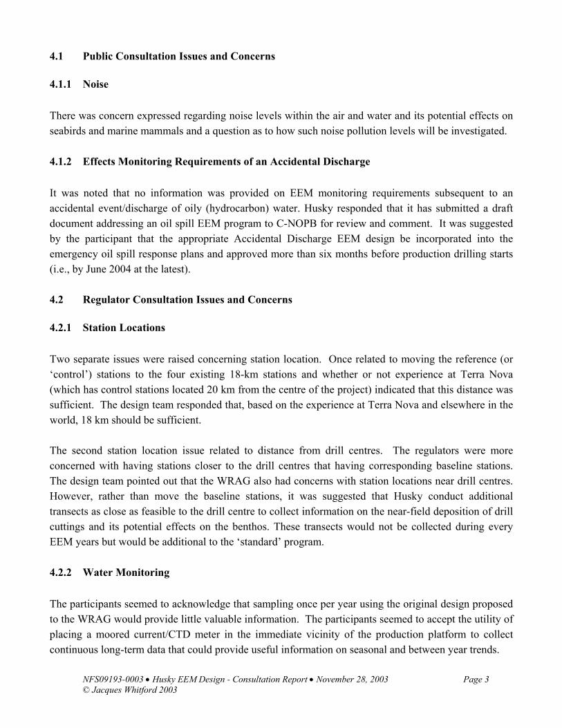
NFS09193-0003 • Husky EEM Design - Consultation Report • November 28, 2003 Page 3© Jacques Whitford 2003
4.1 Public Consultation Issues and Concerns
4.1.1 Noise
There was concern expressed regarding noise levels within the air and water and its potential effects onseabirds and marine mammals and a question as to how such noise pollution levels will be investigated.
4.1.2 Effects Monitoring Requirements of an Accidental Discharge
It was noted that no information was provided on EEM monitoring requirements subsequent to anaccidental event/discharge of oily (hydrocarbon) water. Husky responded that it has submitted a draftdocument addressing an oil spill EEM program to C-NOPB for review and comment. It was suggestedby the participant that the appropriate Accidental Discharge EEM design be incorporated into theemergency oil spill response plans and approved more than six months before production drilling starts(i.e., by June 2004 at the latest).
4.2 Regulator Consultation Issues and Concerns
4.2.1 Station Locations
Two separate issues were raised concerning station location. Once related to moving the reference (or‘control’) stations to the four existing 18-km stations and whether or not experience at Terra Nova(which has control stations located 20 km from the centre of the project) indicated that this distance wassufficient. The design team responded that, based on the experience at Terra Nova and elsewhere in theworld, 18 km should be sufficient.
The second station location issue related to distance from drill centres. The regulators were moreconcerned with having stations closer to the drill centres that having corresponding baseline stations.The design team pointed out that the WRAG also had concerns with station locations near drill centres.However, rather than move the baseline stations, it was suggested that Husky conduct additionaltransects as close as feasible to the drill centre to collect information on the near-field deposition of drillcuttings and its potential effects on the benthos. These transects would not be collected during everyEEM years but would be additional to the ‘standard’ program.
4.2.2 Water Monitoring
The participants seemed to acknowledge that sampling once per year using the original design proposedto the WRAG would provide little valuable information. The participants seemed to accept the utility ofplacing a moored current/CTD meter in the immediate vicinity of the production platform to collectcontinuous long-term data that could provide useful information on seasonal and between year trends.

NFS09193-0003 • Husky EEM Design - Consultation Report • November 28, 2003 Page 4© Jacques Whitford 2003
One of the participants questioned whether or not the water quality monitoring program was a gradientdesign and if the null hypothesis for water quality was still valid. The design team responded that thenull hypothesis, which implicitly calls for a gradient design, would be address shortly before release ofproduced water. It was also confirmed that there is no real vertical component to the plume, exceptimmediately upon release. In addition, another participant pointed out that the EEM program’semphasis is on biological effects and specifically fish health, which will provide some indicators onwater quality.
4.2.3 Subsea Infrastructure
The C-NOPB pointed out that the current location of subsea infrastructure is unknown and needs to betaken into account before deletion of baseline stations, especially as relates to the northern drill centre.It would appear that station number 37, which has been retained in the current EEM design, could belost due to the potential location of flowlines from the more southern drill centres. If this is the case,then an alternative station should be sampled around this drill centre.
4.2.4 Sand Lance
The participants wanted to know the rationale for not using sand lance as a monitoring species. Thedesign team responded that there is too little known about sand lance to make it an effective monitoringspecies. One participant added that sand lance are much shorter lived than American plaice and are notof commercial value. It was also added that American plaice is currently used as a monitoring species inboth the Hibernia and Terra Nova EEMs. The design team voiced some concern about samplingAmerican plaice given the state of this resource in the project area. Participants felt the resource wasrecovering, although slowly.
4.2.5 Future Activities
Husky indicated that based on the delineation well drilling Husky has recently conducted, the potentialexists that Husky could excavate a fourth drill centre 5 km south of the southern glory hole. Huskyacknowledged that if this happens, there would be modifications to the EEM design to accommodate thenew drill centre. In addition, Husky acknowledged that the fourth drill centre could have an impact onthe southeast and southwest reference stations.
5.0 REFERENCES
C-NOPB (Canada-Newfoundland Offshore Petroleum Board). 2001. Decision 2001.01: Applicationfor Approval – White Rose Canada-Newfoundland Benefits Plan and White Rose DevelopmentPlan. St. John’s, NL. iii + 185 pp.

NFS09193-0003 • Husky EEM Design - Consultation Report • November 28, 2003 Page 5© Jacques Whitford 2003
Hodgins, D.O. and S.L.M. Hodgins. 2000. Modelled Predictions of Well Cuttings Deposition andProduced Water Dispersion for the Proposed White Rose Development. Part Two Document bySeaconsult Marine Research Ltd. for Husky Oil Operations Limited. 45 pp.
Husky Oil Operations Limited. 2000. White Rose Oilfield Comprehensive Study - Part One:Environmental Impact Statement. Submitted to the Canada-Newfoundland Offshore PetroleumBoard, St. John’s, NL.
NEB, C-NOPB and C-NSOPB (National Energy Board, Canada-Newfoundland Offshore PetroleumBoard and Canada-Nova Scotia Offshore Petroleum Board). 2002. Offshore Waste TreatmentGuidelines.

APPENDIX C
Statistical Analysis

NFS09193 • Appendix C - Statistical Analyses • May 11, 2004 Page C-1© Jacques Whitford 2004
Sediment Quality
Primary Analysis
Single Sample Year
Analyses for single EEM sample years will be similar to those used for the baseline survey and in theTerra Nova EEM program. Basic analyses will consist of calculation of summary statistics (minima,maxima, means, standard deviation, etc.) over all sample stations, distance regressions, and correlationswithin and among SQT components. Other analyses will occasionally be conducted to refine methods.
For the baseline survey, three X variables were used for regression analysis of SQT or Y variables:
• distance from the centre of the development (i.e., from the original proposed floating production,storage and offloading (FPSO) facility location);
• direction from the centre (expressed as cos and sin θ, with θ the angle relative to due north); and• depth (which increases to the east).
The baseline analysis used distances and directions from a single “source”, the proposed FPSO location.In the EEM program, direction variables will probably be unnecessary. If distances from each of thethree drill centres are used as X variables, directional effects can be inferred from the magnitude ofeffects from each source (=triangulation). If directional effects are limited, a single X variable (distancefrom the nearest drill centre, or the nearest of the southeast and southwest drill centres, as in Table 2.2and Appendix E) may be adequate. Depth will be included in regression analyses because there weresome significant baseline depth effects.
Distance regressions describe the magnitude and spatial extent of contamination or effects. Theregressions can be used to predict Y values at any distance or location, and compare those values toreference values or standards (e.g., sediment quality criteria or effects concentrations). Similarly, inverseprediction (prediction of X from Y) can be used to determine distances at which reference values,standards, or other Y values occur or are exceeded.
Correlational analyses of SQT data focus on relationships within and especially among components (i.e.,chemical and physical characteristics, toxicity, benthic infaunal communities). The primary objective isto determine if contamination (or physical alterations) and biological effects are correlated (=stress- ordose-response relationships). Correlations within SQT components are used to assess if there aregeneralized patterns or “syndromes” of contamination or effects, and to develop summary measures foreach component (i.e., correlations are expected within each component, especially when contaminationand effects occur).

NFS09193 • Appendix C - Statistical Analyses • May 11, 2004 Page C-2© Jacques Whitford 2004
In the White Rose baseline, Spearman non-parametric rank correlations (rs) were used to calculatebivariate correlations between variables within SQT components. Using rs is a universal approach thatavoids any need to make transformations, and non-parametric methods can be as powerful as parametricmethods with larger sample sizes (i.e., n>10). Kendall's non-parametric Coefficient of Concordance (W)can be used to calculate the overall or multiple correlation among v>2 variables.
In the White Rose baseline report, relationships among SQT components were examined using amultivariate approach suggested by Green et al. (1993), and used by Chapman et al. (1996) for an SQTstudy of sewage discharge effects. Briefly, matrices of multivariate pair-wise distances between stationswere calculated for each SQT component, then correlations among those distance matrices tested. Greenet al. (1993) discuss other approaches for analyzing SQT data.
Multiple Sample Years
Repeated Measures (RM) distance regressions will be used to analyze data from multiple years. RMregressions are the same as single-year regressions, except that Y is some combination of values frommultiple years. For example, after the first EEM sample year, Y could be the EEM value minus thebaseline value (or vice versa) or the before-after (BA) difference. Significant regressions of BA ondistance from active drill centres would indicate that distance gradients changed after drilling started,which is usually evidence of contamination or effects. RM designs and analyses are most effective whenthere are strong carry-over effects, or persistent differences among stations over time unrelated todistance (or other X variables of interest).
For comparisons of EEM values to before or baseline values, using the before values as an additional Xvariable in multiple regression will always be more powerful than differencing (i.e., subtracting ordividing by baseline values) (Cohen 1988; Everitt 1994). Treating the before and after values as multipleY values in multivariate regression will also be more powerful than differencing. These two alternativeseffectively use different weights for the before and after values to maximize the relationship betweenBA and distance, whereas differencing weights before and after values equally. However, the standardRM model and approach, which is based on differencing, is more flexible, more informative, andpreferred when there are greater than two years and several comparisons of interest.
Correlations among SQT variables over multiple years can also be examined. If natural changes overtime are small, data from all years can be pooled and analyses conducted as for single years, but withmuch larger sample sizes. This approach can be effective for collapsing more complex RM distanceregressions when contamination is not a simple function of distance from drill centres, or when thetiming or intensity of drilling activity varies among drill centres or years. If natural changes over yearsare larger, correlations can be compared among years. Carry-over effects can be accommodated bysubtracting or dividing by baseline values, or more generally, by analyzing differences or othercombinations of values over multiple years.

NFS09193 • Appendix C - Statistical Analyses • May 11, 2004 Page C-3© Jacques Whitford 2004
Secondary Analysis
At the request of regulators, aluminum normalization will also be used to assess barium concentrationsin sediments. Concentrations of barium in uncontaminated marine sediments will usually be positivelycorrelated with concentrations of other metals, as they were in the baseline survey. Thus, “expected”barium concentrations in the absence of contamination from water-based drilling muds (WBM) can bepredicted from concentrations of other metals that are largely unaffected by drilling. Aluminum istypically used as a predictor, because it occurs naturally at high concentrations in marine sediments, andis not a major constituent of drilling muds.
The first step is to develop a baseline barium-aluminum regression. Barium concentrations in EEMyears are then compared to values predicted by aluminum concentrations in the same sediments, usingthe baseline regression. Higher-than-predicted barium concentrations would be considered evidence ofcontamination from WBM. If distance gradients for barium contamination were of interest, observedminus predicted barium concentrations could be regressed on distance.
Aluminum normalization is a potential alternative to repeated measures (RM) approaches, in whichbaseline barium concentrations, rather than aluminum concentrations, are used as predictors of EEMbarium concentrations. Aluminum normalization will be most effective when:
• carry-over effects are weak, and baseline barium concentrations poor predictors of EEM bariumconcentrations; and/or
• baseline barium concentrations are unavailable (e.g., for the three near-field EEM stations notsampled in baseline).
Otherwise, RM approaches, which are effectively “baseline normalization”, are preferred, because theycan be applied to analysis of many other sediment quality variables.
Commercial Fish
Analyses of commercial fish data from single years will include:
• calculation of summary statistics for each Area;• comparison of American plaice and snow crab body burdens among Areas in ANOVA;• comparison of taste results between Study and Reference Areas in ANOVA or t tests;• comparison of American plaice health indicators among Areas in ANOVA; and• comparison of American plaice and snow crab biological characteristics (e.g., sex ratios, size, age)
among Areas, and among trawls or composites within Areas.

NFS09193 • Appendix C - Statistical Analyses • May 11, 2004 Page C-4© Jacques Whitford 2004
With four Reference Areas, two comparisons or contrasts are of primary interest:
• Among References, and• Study Area versus References.
Given the size of the Study Area, comparisons between the northern and southern portion of the StudyArea are also of interest and can be performed given sample sizes and distribution of collection sitesproposed in this document.
Differences among Reference Areas represent natural large-scale spatial differences. Differencesbetween the northern and southern portion of the Study Area could represent natural differences ordifferences in the extent or magnitude of project effects. One would conclude that the differences werenatural if they were similar to differences among the Reference Areas. The difference between the StudyArea and the overall or grand Reference mean is a measure of potential effects, and is also known as theControl-Impact or CI difference. The three contrasts can be tested in most statistical packages (e.g.,SYSTAT, SPSS) following an ANOVA. Alternatively, the four Reference Areas can first be comparedin an ANOVA, and the northern and southern portion of the Study Area can be compared in a t test. Thefour References would then be pooled as a single “Area” for comparison to the Study Area. That is theapproach that would be used for analysis of frequencies (e.g., sex ratios or incidences of abnormalities)in log-likelihood or G tests (similar to χ2 tests; Sokal and Rohlf 1981; Paine 1998).
The tests described above use composites or individual American plaice or snow crab within Areas asreplicates, and assume that there is no added natural large-scale variance among Reference Areas orbetween the northern and southern portion of the Study Area. If there are differences among theReference Areas, Areas are the appropriate replicates for testing the Study versus Reference contrast.Comparisons among Areas would then be made in nested ANOVA, with Areas as replicates within“Reference” and “Study” groups, and composites or individual American plaice or snow crab (i.e.,subsamples) as replicates within groups. The northern and southern portion of the Study Area would betreated as separate groups if differences between them were greater than differences among theReferences. Replication (i.e., >1 Area) is not required within the Study group, provided that there aremultiple References. Winer (1971) suggests that variance among Areas within groups can be pooledwith the variance among subsamples (i.e., subsamples rather than Areas can be used as replicates fortesting the Study versus Reference contrast) when p>0.20 for the Among References test or contrast.When differences among References are larger, or significant at lower p (p<0.20 and especially <0.05),the magnitude and potential causes of those natural differences may be more relevant than the statisticalsignificance of the Study versus Reference contrast, however tested.
In the White Rose EEM program, American plaice and snow crab size and other biologicalcharacteristics could be compared among trawls or composites within Areas, as well as among Areas.Nested ANOVA, with Area and Trawls within Areas as terms or sources of variance, could be used for

NFS09193 • Appendix C - Statistical Analyses • May 11, 2004 Page C-5© Jacques Whitford 2004
analysis of size, for example. The objective of these analyses would be to estimate smaller-scalevariance among trawls, and the legitimacy of protocols or procedures used for pooling or compositingAmerican plaice or snow crab within Areas. Variance among trawls or composites within Areas is notexpected to be large for mobile fish or shellfish, but that assumption should be tested whenever possible.
In EEM programs, it is usually preferable to sample the same Areas both before and after project activity(e.g., drilling) occurs. With a single Reference Area and a single Study Area, this is a Before-AfterControl-Impact (BACI) design (Green 1979). The test for effects is then a test for a change in the CI(Study versus Reference) difference between before and after years, with the before or baseline CIdifference providing an estimate of natural variance among Areas. In the baseline survey, differences inbody burdens and American plaice health indicators between the Northwest Reference and the StudyArea fish were measured, but:
• sediment chemistry and benthic invertebrate communities differed significantly between the twoAreas;
• sample sizes for body burden analyses were limited for American plaice; and• Reference snow crab were sampled two years after Study Area snow crab.
Ideally, the four 28 km References as well as the Study Area would have been sampled in the baselinesurvey. However, it was not known in 2000 (the baseline sampling year) that the Northwest ReferenceArea was not comparable to the Study Area. The baseline Study Area sampled also did not extend as faras the new NN and SS drill centres. The multiple-reference design effectively replaces the baselineestimate of natural variance between Areas with an estimate (the Among References contrast) madeeach EEM or after year. As EEM data accumulate, changes in the Study versus Reference contrast ordifference with intensification and then cessation of drilling activity may be of interest, and can beassessed in two-way ANOVA with Year and Area as factors.
In the Terra Nova EEM, there have been few or no consistent differences in American plaice healthbetween the Study and Reference Areas, so quantitative comparisons among years have not beenwarranted or conducted. Body burdens have been compared over both time (Years) and space (Areas).

APPENDIX D
Statistical Power and Robustness

NFS09193 • Appendix D - Statistical Robustness & Power • May 11, 2004 Page D-1© Jacques Whitford 2004
Statistical Power and Robustness
Overview
Statistical power (P) is the probability that an effect of a specified size (=target effect size (ES)) will bedetected in samples if it exists in the real world. Real-world or population effects can only be estimatedfrom samples; their precise values are never known. Because of sampling error or uncertainty, real-world effects may go statistically undetected (=Type II error, with probability β (or 1−P)). Target ESmust be specified to calculate P; it is incorrect to assume that power refers to the probability of detectingany non-zero effect (i.e., ES≠0). Small effects will always occur and go undetected in samples. Forexample, release of one hydrocarbon molecule is an effect that would never be detected.
An effect in samples may be statistically significant when the target ES does not exist in the real world(=Type I error). The probability of a Type I error is α, with α typically set at 0.05 (or 5 percent) (i.e.,results are not considered statistically significant unless p≤0.05). The probability that the target ES, if itdoes not occur, will not be statistically significant is then 1−α.
Combinations of real-world ES and results of statistical tests conducted on samples, and theirprobabilities, are summarized in Table 1. In environmental monitoring programs, the objective should beto minimize both Type I and Type II errors. Type I errors are potentially damaging to proponents (e.g.,industry, dischargers), if they have to pay for unnecessary clean-up or remediation. Type II errors arepotentially damaging to the environment, if large effects go undetected. Minimizing both Type I andType II errors maximizes the probability of making correct conclusions about real world effects (Table1).
Table 1 Outcomes and Their Probabilities for Sample Estimates of Real-World Effects
Real-worldSample resultsES<target ES ES≥target ES
Observed ES not significant Correct(probability = 1−α)
Type II error(probability = 1−P = β)
Observed ES significant Type I error(probability = α)
Correct(probability = P)
NOTE: ES=Effect Size

NFS09193 • Appendix D - Statistical Robustness & Power • May 11, 2004 Page D-2© Jacques Whitford 2004
P increases with increasing sample size (n), increasing ES (i.e., larger effects are easier to detect),increasing α, and decreasing error variance (i.e., variance unrelated to the effect of interest). Because αis usually fixed at 5 percent (or 0.05), power analyses usually focus on examining various combinationsof n, P, or ES. Beyond n=10, variance and sample size are inversely related. Reducing variance by afactor of two, for example, provides the same increase in power as doubling sample size, and is usuallyconsiderably less costly and more practical. The emphasis should be on developing better samplingdesigns, field and laboratory procedures, and statistical analyses that reduce error variances and betterestimate real-world effects, rather than on increasing n.
Robustness is also important. Robust results are informative, reliable, repeatable, and potentiallyapplicable to other situations or scenarios (=generality). There is often a trade-off between power for aspecific purpose or ES, and information and generality. For example, a basic Control-Impact (CI) designcomparing the Study Area to a single Reference may be powerful enough to detect relatively small CIdifferences (=ES), but only between those two Areas. A regression design with the same overall samplesize would provide a poorer estimate and test of that specific CI difference, but would add informationon effects at intermediate exposure levels. Similarly, a multiple-reference design would provide aweaker test of the difference between the Study Area and a specific or single Reference, but additionaltests or estimates of natural variance among multiple References, and a more robust comparison of theStudy Area to Reference Areas in general.
Sediment Quality Survey
For the sediment quality survey regression and correlation analyses, ES can be expressed as correlations,with ρ representing real-world correlations estimated by observed or sample correlations (or r (or non-parametric equivalents)). ρ2 is the proportion of variance in Y attributable to variance in X. 1−ρ2 is theerror variance as a proportion of the total variance in Y.
From a practical or operational perspective, reducing error variance is equivalent to increasing ρ. Real-world effects (or ρ) do not depend on sampling designs, technical methods or data analyses, but thosefactors affect sample estimates of real-world effects. Suppose that sample or observed r=0.3 for Method1 (e.g., for some design, field method or statistical analysis) and 0.5 for Method 2. Method 2 is morepowerful, although both methods estimate the same real-world effect (or ρ). Method 2 may provide abetter “picture” or model of reality than Method 1, because it:
• uses a more appropriate statistical model (e.g., an X variable that explains more variance in Y);• eliminates or reduces some sampling variance (e.g., due to field or laboratory practice) that does not
exist in the real world; or• explains or removes some real natural variance (i.e., some portion of 1−ρ2) attributable to factors
other than X variables of interest.

NFS09193 • Appendix D - Statistical Robustness & Power • May 11, 2004 Page D-3© Jacques Whitford 2004
Bivariate Regression and Correlation in a Single Year
The relationship between detectable ES or ρ and sample size for P=95 percent and α=0.05 (or 5 percent)(i.e., with α=β=5 percent) (left plot), and the relationship between P and n for selected ρ (right plot), areprovided in Figure 1. Increasing sample size provides ever-diminishing returns, in terms of reducingdetectable ES or increasing P, as illustrated in Figure 1. The curves are asymptotic, with the greatestgains in power (steepest slopes) achieved at small sample sizes.
Figure 1 Statistical Power for Analysis of Distance Gradients and Other Correlations (ρ)
With n≥48 (as for baseline collection and the proposed EEM design), there is a high probability (P>99pecent) that ρ=0.7 (ρ2≈0.5) will be detected. In the White Rose baseline survey, r for natural distancegradients and relationships between SQT components were generally <0.7. Even at contaminated sites,correlations among SQT components may be <0.7 (e.g., Green et al. 1993; Green and Montagna 1996).
Prohibitively large sample sizes (n≥80 stations) would be required to provide a ≥80 percent probabilityof detecting lower ES such as ρ=0.3 (Figure 1). With n≥48, the probability of detecting ρ=0.3 isapproximately 50 percent (Figure 1, right plot). Correlations of this strength, with X accounting for <10percent of the variance in Y, have little predictive or explanatory power, and may be lower than many rfor natural distance gradients and correlations among SQT variables.
For any given n, the power of regression or correlation analysis also increases as the variance or range ofX values increases. Increasing the variance of X effectively reduces 1–ρ2, or explains more of thevariance in Y than a narrower range of X values. For example, the observed or sample r based on Xvalues ranging between 1 and 10 is likely to be greater than r based only on X values between 5 and 6.For that reason, stations representing extreme values of X (e.g., distance) may be more “valuable” than
0 50 100 150
Sample size
0.2
0.4
0.6
0.8
1.0
Det
ecta
ble
corre
latio
n Power=95%
0 20 40 60 80
Sample size
102030405060708090
100
Pow
er (%
)
ρ=0.3
ρ=0.7
ρ=0.5

NFS09193 • Appendix D - Statistical Robustness & Power • May 11, 2004 Page D-4© Jacques Whitford 2004
stations representing intermediate values. That was the rationale for adding the three near-field stations250 m of drill centres, which represent extreme or low distance values (=worst case). The addition offour far-field stations at 28 km also increases power.
Multiple Regression
With multiple X variables in distance regressions, the power curves in Figure 1 shift to the right, becauseadding variables reduces error degrees of freedom and effective sample size. However, if the effects ofthe different X variables on Y are relatively independent, error variances will be reduced relative tobivariate regression. ρ or ρ2 effectively increases, and power may increase for any n. In the White RoseEEM program, including depth in distance regressions should reduce error variances and increase powerfor analyses of some SQT variables.
Multiple Years
The power curves in Figure 1 also apply to Repeated Measures (RM) regression for multiple years, withY some combination of single-year values. The power of RM analyses depends on the particular timecombination of interest. Power usually increases as the number of years included in the comparisonincreases. Power will be greater for tests on means than for tests on differences. Power will also begreater for more balanced comparisons (e.g., two EEM or after years versus two other EEM years, asopposed to the mean of all four years versus a single baseline year).
For the first EEM year, regressions of after (EEM) minus before (baseline) values (=before-after (BA)differences) on distance will be of primary interest (see Appendix C). Sample size remains the same asfor a single year, because there will be one BA difference for each of the 37 stations sampled in baseline(i.e., n=37 not 74). Detectable ES or P for any ES also remain the same. However, those ES represent ρbetween BA differences, not single-year values, and X. Baseline, or natural distance gradients, havebeen removed, so ρ or sample r for BA are better or “purer” measures of effects than single-yearcorrelations. There is less risk that natural correlations for BA (presumably approximately 0) will bemisinterpreted as effects (i.e., reliability and robustness increase).
A correlation of differences is also a difference in correlations, although correlations are not strictlyadditive. Given that:
• natural correlations for BA regressions should be approximately 0; and• the suggested target ES of ρ=0.5 for single years was based on the assumption that natural
correlations within years were non-zero.
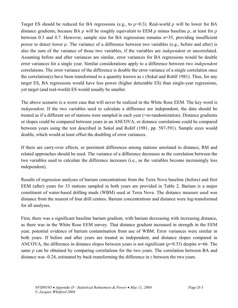
NFS09193 • Appendix D - Statistical Robustness & Power • May 11, 2004 Page D-5© Jacques Whitford 2004
Target ES should be reduced for BA regressions (e.g., to ρ=0.3). Real-world ρ will be lower for BAdistance gradients, because BA ρ will be roughly equivalent to EEM ρ minus baseline ρ, at least for ρbetween 0.3 and 0.7. However, sample size for BA regressions remains n=35, providing insufficientpower to detect lower ρ. The variance of a difference between two variables (e.g., before and after) isalso the sum of the variance of those two variables, if the variables are independent or uncorrelated.Assuming before and after variances are similar, error variances for BA regressions would be doubleerror variances for a single year. Similar considerations apply to a difference between two independentcorrelations. The error variance of the difference is double the error variance of a single correlation oncethe correlation(s) have been transformed to a quantity known as z (Sokal and Rohlf 1981). Thus, for anytarget ES, BA regressions would have less power (higher detectable ES) than single-year regressions,yet target (and real-world) ES would usually be smaller.
The above scenario is a worst case that will never be realized in the White Rose EEM. The key word isindependent. If the two variables used to calculate a difference are independent, the data should betreated as if a different set of stations were sampled in each year (=re-randomization). Distance gradientsor slopes could be compared between years in an ANCOVA, or distance correlations could be comparedbetween years using the test described in Sokal and Rohlf (1981, pp. 587-591). Sample sizes woulddouble, which would at least offset the doubling of error variances.
If there are carry-over effects, or persistent differences among stations unrelated to distance, RM andrelated approaches should be used. The variance of a difference decreases as the correlation between thetwo variables used to calculate the difference increases (i.e., as the variables become increasingly lessindependent).
Results of regression analyses of barium concentrations from the Terra Nova baseline (before) and firstEEM (after) years for 33 stations sampled in both years are provided in Table 2. Barium is a majorconstituent of water-based drilling muds (WBM) used at Terra Nova. The distance measure used wasdistance from the nearest of four drill centres. Barium concentrations and distance were log-transformedfor all analyses.
First, there was a significant baseline barium gradient, with barium decreasing with increasing distance,as there was in the White Rose EEM survey. That distance gradient increased in strength in the EEMyear, potential evidence of barium contamination from use of WBM. Error variances were similar inboth years. If before and after years are treated as independent, and distance slopes compared inANCOVA, the difference in distance slopes between years is not significant (p=0.33) despite n=66. Thesame p can be obtained by comparing correlations for the two years. The correlation between BA anddistance was -0.24, estimated by back-transforming the difference in z between the two years.

NFS09193 • Appendix D - Statistical Robustness & Power • May 11, 2004 Page D-6© Jacques Whitford 2004
Table 2 Example Analyses of Terra Nova Baseline (before) and First EEM Year (after)Barium Concentrations
Model Error df Error variance(× 1000)
Distance gradient(r)
p
Before 31 11.9 -0.426 0.013After 31 10.4 -0.606 <0.001ANCOVA 62 NA −0.241 0.333BA versus distance 31 7.1 -0.298 0.093Before as X 30 5.7 −0.4792 0.006Multivariate 30 NA −0.6083 <0.001NOTES:The first two analyses test within-year concentrations gradients; the last four test for changes in gradients between
years.BA = before-after difference in barium concentrations.Barium concentrations and distance log-transformed for all analyses.n=33 stations sampled in both years.NA = Not Applicable (error variance comparable to other analyses difficult to estimate).
1—estimates assume natural BA gradient (r) would be 0.2—partial correlation between after and distance, with effects of before removed.3—based on 10:1 after:before weighting.
Source: Petro-Canada 2002.
Carry-over effects were highly significant for barium in this example (p<<0.001). The correlationbetween residuals from distance regressions (i.e., with distance effects removed) for the two years wasr=0.69. That r is one of the highest natural correlations observed in the Terra Nova EEM program(except for other carry-over effects and correlations). Consequently, the error variance for a regressionof BA differences on distance was lower than the error variances within each year. The sample estimate(r) of the real-world distance gradient or correlation (ρ) was -0.298, somewhat higher than the estimatebased on assuming before and after values were independent. Thus, power was increased by reducingerror variance and increasing the estimate of ρ. The correlation between BA and distance was notstatistically significant (0.05<p<10), but would be if distances from the two drill centres active at thetime were used as X (arguably a more logical model).
When before, or baseline barium concentrations, were used as an additional X variable in multipleregression, p for regression of EEM, or after values on distance, was highly significant (p=0.006; Table2). Error variance was reduced to approximately half the error variance in either year. The sampleestimate of the partial correlation between EEM values and distance (i.e., with the effects of baselinevalues or carry-over effects removed) was -0.479.
When before and after values were used as multiple Y variables in multivariate regression, resultsindicated that the change in distance gradients was significant at p<0.001 (Table 2). This analysissuggested that a 10:1 before:after weighting maximized the relationship between the BA difference anddistance. Based on that weighting, the correlation between weighted BA and distance increased to -0.61

NFS09193 • Appendix D - Statistical Robustness & Power • May 11, 2004 Page D-7© Jacques Whitford 2004
(similar to r for the EEM year only, which is a 10:0 after:before weighting). The multivariate approachwill usually be more powerful and appropriate than other RM alternatives only when t=2 times or years(Green 1993; Tabachnick and Fidell 1989). With t>2 times, multivariate analysis rapidly loses power,and becomes a “fishing expedition” exploring all possible time combinations.
The analyses in Table 2 required less than two hours to conduct, but the RM design and analyses hadmore power than would re-randomization designs and analyses based on much larger and more costlysample sizes. This is an admittedly extreme example; differences among methods for analyses, andbetween RM and re-randomization design, would be smaller for other SQT variables with weaker carry-over effects. However, RM designs and analyses would still be superior to re-randomization designs andanalyses for most, if not all, SQT variables.
Multivariate Correlation and Other Methods
Multivariate approaches will usually be more robust and powerful than examining bivariate correlationsamong SQT variables. For example, Principal Components Analysis (PCA) was used in the baselinesurvey to derive a single summary measure (effectively a weighted average) of concentrations of 10frequently detected metals in sediments. Even at uncontaminated sites, metal concentrations will usuallybe strongly positively correlated. Using a summary measure such as the first Principal Component (PC1)that reflects those correlations increases:
• power (error variances are lower for a weighted mean than for a single variable or metal); and• generality (i.e., robustness) and efficiency (conclusions based on metal PC1 can be generalized to all
metals, without conducting analyses on 10 different variables or metals).
Kendall's Coefficient of Concordance (W), a multivariate correlation, is less powerful than Spearman'srank correlation (rs) for analysis of correlations between two variables. However, for multiple relatedvariables, W can be more powerful than rs (depending on how one wants to adjust p or α for analyzingmultiple bivariate correlations). A single value of W is also easier to interpret and present than a matrixof bivariate or pair-wise correlations. Paine (1998) showed that testing W among SQT components(chemistry, toxicity, benthic infaunal communities) was as powerful as more complex multivariateapproaches suggested by Green et al. (1993) for some sample Vancouver harbour SQT data. The overallstatus for the 13 stations could be simply expressed by averaging ranks for the three SQT components(or ranking those averages from 1 to 13).
NFS09193 • Appendix D - Statistical Robustness & Power • May 11, 2004 Page D-8© Jacques Whitford 2004
Commercial Fish
The commercial fish survey data will be analyzed in ANOVA comparing Areas and sometimes Years,or equivalent procedures for analyzing frequencies (e.g., sex ratios or incidence of abnormalities). Asnoted in Appendix C, two comparisons or contrasts are of primary interest:
• Among References; and• Study versus Reference.
The power of tests of these two contrasts is considered below. Discussion considers sample sizes of upto five composites for body burden in the Study Area (which would apply to comparison of either thenorthern or southern portion of the Study Area to Reference Areas) and sample sizes of up to 50 fish forhealth indices in the Study Area. Planned sample sizes to 10 composites for body burden and 60 fish forhealth analysis, overall, for the Study Area provide higher power than that reported below. The powerof taste tests is not considered, since that is largely determined by protocols.
For power analysis of fish health indicators and tissue chemistry (body burdens), ES can be standardizedby dividing them by the SD within Areas. The Study versus Reference contrast or difference (=CIdifference) would be the Study Area mean minus the grand mean of the Reference Area means, dividedby the within-Area SD. Overall variance or differences among the four Reference Areas can beexpressed using f, a common power index for ANOVA (Cohen 1988). f is the SD among the ReferenceArea means, divided by the within-Area SD. f can be considered the roughly comparable to the CIdifference, since it is the “average” difference between any single Reference Area and the grand mean ofthe Reference means. General points made for sediment quality for power of analysis of ρ also apply tothe CI difference and f, since both can be converted to correlations or ρ (Cohen 1988).
Body Burdens (Tissue Chemistry)
Detectable f and CI differences (=ES) for power (P) of 50 and 95 percent are given in Table 3 forvarious multiple-reference designs. The ES for P=50 percent are also minimum significant differences(MSD), or the smallest observed differences that would be statistically significant at p≤0.05. The fprovided are for an ANOVA comparing the References only (i.e., with the Study Area excluded).Detectable f would be slightly lower if the Among References contrast were tested using the error anderror df from an ANOVA comparing all Areas, but power for that contrast is difficult to calculate exceptby simulation. Detectable CI apply to a test of the Study versus Reference contrast using the error anderror df from an ANOVA comparing all Areas.

NFS09193 • Appendix D - Statistical Robustness & Power • May 11, 2004 Page D-9© Jacques Whitford 2004
Table 3 Detectable Effect Sizes (ES) for Analyses of Commercial Fish and Shellfish BodyBurdens
Detectable Effect Size (SD units)Among References
(f)Study versus Reference
(CI difference)
Design No.Ref.
Areas
nR nS Totalsample
sizePower=50% Power=95% Power=50% Power=95%
1 4 2 3 11 1.36 2.50 1.66 2.972 4 2 4 12 1.36 2.50 1.45 2.613 4 2 5 13 1.36 2.50 1.31 2.374 4 3 3 15 0.88 1.55 1.44 2.615 4 3 4 16 0.88 1.55 1.27 2.316 4 3 5 17 0.88 1.55 1.16 2.117 3 2 3 9 1.55 >2.5 1.82 3.248 3 2 4 10 1.55 >2.5 1.58 2.839 3 2 5 11 1.55 >2.5 1.43 2.5810 3 3 3 12 0.96 1.75 1.54 2.7811 3 3 4 13 0.96 1.75 1.36 2.4612 3 3 5 14 0.96 1.75 1.24 2.25CI 1 5 5 10 Not Applicable 1.46 2.63NOTES: nR=no. composites per Reference Area; nS=no. composites in Study Area
SD=SD within Areas
In Table 3, ES are provided for designs with Reference sample sizes (nR) of two or three composites perArea, and Study Area sample sizes (nS) of three to five composites. ES are provided for three as well asfour References, to account for the possibility that one Reference may not provide adequate numbers ofAmerican plaice or snow crab, or may not be physically or biologically similar to other Areas (i.e.,excluded from analyses). Detectable CI differences are also provided for a basic CI design comparingthe Study Area to a single Reference, with n=5 composites within each Area. These are the sample sizesused in the Terra Nova EEM CI design.
Detectable f for the comparison among References decrease substantially when nR increases from two tothree (Table 3). With only two composites per Area, detectable f are not much smaller than detectable CIdifferences. Therefore, the CI difference or Study versus Reference contrast could be statisticallysignificant when differences among References that are not much smaller are not statistically significant.With three composites per Reference Area, detectable f are much smaller than detectable CI differences.
The Study Area sample size (nS) has no effect on the power of the test of the Among Referencescontrast, except to slightly increase error df from an ANOVA comparing all Areas. Therefore, the“optimal” Study Area sample size for a test of the Among References contrast is 0. However, for a testof the CI difference or Study versus Reference contrast, the optimal allocation is to use approximatelyequal numbers of Reference and Study Area samples (i.e., ΣnR≈nS or nS≈rnR where r is the number ofReference Areas). Once ΣnR≥nS, increasing Reference sample sizes is not as cost-effective as increasingStudy Area sample sizes. For example, Design 4 in Table 3, with three composites per Area and a totalof 15 composites, is less powerful for a test of the CI difference than Design 3, with two composites

NFS09193 • Appendix D - Statistical Robustness & Power • May 11, 2004 Page D-10© Jacques Whitford 2004
within each Reference Area, five composites within the Study Area, and a total of 13 composites.However, Design 4 provides a much more powerful test of the Among References contrast.
Given that there is a conflict between optimal sampling allocations for the two contrasts of interest, andno a priori reason to consider one contrast more important than the other, Design 6 in Table 3, withnR=3 composites in each Reference Area and nS=5 composites in the Study Area, is a reasonablecompromise for the White Rose EEM program. That design provides more power for a test of the CIdifference than the basic or more traditional CI design with a single Reference, and a more powerful testof natural differences among References than any design with only two composites per Reference Area(Table 3). Sample sizes for Design 6 should be regarded as target sample sizes, since failure to achievethem in every Area should still provide a reasonably powerful test of both spatial contrasts of interest.Larger sample sizes would provide more power, but, assuming that 10 American plaice or snow crab arerequired per composite, would probably be unachievable or unacceptable in terms of sampling mortality.
If differences among References are large (i.e., p≤0.20 and especially ≤0.05 for the Among Referencescontrast), the one versus many t test or a nested ANOVA is appropriate for testing the CI difference orStudy versus Reference contrasts (Appendix C). Sample sizes would then be the number of ReferenceAreas. With only three or four Reference Areas, those tests have little power. The CI or Study versusReference difference would usually not be statistically significant unless the Study Area mean wereoutside the range of Reference means, and much larger than the MSD or detectable differences forP=0.5 in Table 3. The number of Reference Areas would have to be increased to increase power, whichmight not be feasible. When there are large differences among multiple references, the statisticalsignificance of the Study versus Reference contrast, however tested, may be of minor interest. Importantquestions should be:
1. Are one or more Reference Areas inappropriate for comparison to the other Reference Areas and theStudy Area?
2. Are Study versus Reference or CI differences (i.e., potential effects), regardless of statisticalsignificance, trivial relative to naturally occurring differences among apparently similar ReferenceAreas?
When data from multiple (i.e., t) EEM years are analyzed in two-way ANOVA with Year and Area asfactors, effective sample sizes for tests of consistent spatial differences (e.g., Among References; Studyversus Reference) increase by a factor of approximately t. In other words, years are an additional formof replication. However, changes in spatial differences or contrasts, particularly the CI difference, overtime may be of more interest. These are tests of Year × Area interactions, and like any tests ofdifferences, will have less power than tests of main effects (Year or Area).

NFS09193 • Appendix D - Statistical Robustness & Power • May 11, 2004 Page D-11© Jacques Whitford 2004
Fish Health Indicators
Detectable ES or f among References and CI differences are provided in Table 4. Designs are the sameas those in Table 3 for body burden analysis, with sample sizes multiplied by 10, assuming that 10American plaice would be required per composite. The ES in Table 4 also apply to analysis of anyvariable (e.g., size) measured on individual snow crab. Satisfying minimal or recommended samplesizes for body burden analysis should provide more than adequate power for most analyses of fish healthindicators and other variables measured on individual American plaice or snow crab. Even if that werenot true, further increases in sample sizes would not substantially increase power. With sample sizes of20 to 50 American plaice or snow crab per Area, and four or five Areas, power curves for f or the CIdifference converted to ρ would be towards the right half of the two plots in Figure 1.
Table 4 Detectable Effect Sizes (ES) for Analyses of Commercial Fish Health Indicators
Detectable Effect Size (SD units)Among References
(f)Study versus Reference
(CI difference)
Design No.Ref.
Areas
nR nS Totalsample
sizePower=50% Power=95% Power=50% Power=95%
1 4 20 30 110 0.275 0.476 0.424 0.7802 4 20 40 120 0.275 0.476 0.384 0.7053 4 20 50 130 0.275 0.476 0.357 0.6564 4 30 30 150 0.223 0.385 0.403 0.7415 4 30 40 160 0.223 0.385 0.361 0.6636 4 30 50 170 0.223 0.385 0.332 0.6117 3 20 30 90 0.295 0.521 0.445 0.8168 3 20 40 100 0.295 0.521 0.405 0.7449 3 20 50 110 0.295 0.521 0.380 0.69710 3 30 30 120 0.239 0.422 0.418 0.76711 3 30 40 130 0.239 0.422 0.376 0.69112 3 30 50 140 0.239 0.422 0.349 0.641CI 1 50 50 100 Not Applicable 0.397 0.729NOTES: nR=no. fish per Reference Area; nS=no. fish in Study Area
SD=SD within Areas
All designs in Table 4 provide sufficient power to detect relatively small differences (i.e., f<0.3) amongfour or three Reference Areas, and reasonable power to detect CI differences. For example, Design 8,with a total of 100 American plaice and a sampling allocation of approximately ΣnR=nS, provides almostas much power for a test of the CI difference as a basic single-reference CI design with the same numberof American plaice, plus a powerful test of differences among References. Design 6, recommended forbody burden analysis, provides a more powerful test of the CI difference than the single-reference CIdesign, even if target sample sizes cannot be achieved in every Area (e.g., as in Designs 12 or 5).

NFS09193 • Appendix D - Statistical Robustness & Power • May 11, 2004 Page D-12© Jacques Whitford 2004
As for analysis of body burdens, the one versus many t test using Reference Areas as replicates willhave less power for a test of the Study versus Reference contrast than tests using individual fish orshellfish within Areas as replicates. The CI difference is unlikely to be significant unless the Study Areamean lies outside the range of Reference means. However, with nR≈30 fish within the Reference Areas,the range of Reference means may be narrow when the Among References contrast is significant atp≤0.20 or even p≤0.05. For example, the Among References contrast would be significant at p=0.05 if for the SD among Reference means were 0.20 to 0.25 times the SD within Areas (see values for P=0.5 inTable 4). That would represent a range of Reference means 0.4 to 0.8 times the within-Area SD, sincethe range is typically two to three times f (Cohen 1988). If the Study Area mean was within that range,one could legitimately question whether any effects were environmentally significant, even if the Studyversus Reference or CI difference were statistically significant.

APPENDIX E
GPS Coordinates of EEM Sediment Stationsand Distance to Drill Centres

Table 1 GPS Coordinates of EEM Sediment Transect Stations and Distance to Drill Centres
Distance (km) from Drill CentresStation
Easting UTM(NAD83)
Northing UTM(NAD83) N C S NN SS Nearest
20 725,772.67 5,186,341.88 7.76 0.35 3.41 10.20 7.69 0.3513 727,834.64 5,184,425.08 10.22 2.73 0.59 12.20 5.34 0.5931 727,366.46 5,196,401.29 4.20 10.52 12.43 1.10 17.31 1.1016 727,072.34 5,185,666.32 8.79 1.49 2.04 10.89 6.68 1.499 729,839.69 5,184,237.92 11.29 4.58 1.61 12.80 5.30 1.6114 727,912.97 5,182,365.06 12.18 4.31 1.67 14.26 3.28 1.678 728,457.98 5,185,685.16 9.35 2.85 1.70 11.06 6.56 1.7017 725,699.77 5,184,198.36 9.85 1.83 2.56 12.34 5.77 1.8323 727,073.01 5,187,136.89 7.43 1.83 3.35 9.43 8.13 1.8321 723,752.16 5,186,266.73 7.64 1.89 5.04 10.57 8.54 1.8930 727,450.25 5,194,601.93 3.52 8.77 10.63 2.26 15.51 2.2624 725,683.95 5,188,599.44 5.56 2.58 5.27 7.95 9.87 2.5815 728,146.12 5,176,433.04 17.95 9.92 7.57 20.18 2.71 2.715 729,768.87 5,186,492.52 9.39 4.17 2.92 10.63 7.49 2.921 728,436.36 5,187,144.12 8.08 3.03 3.15 9.63 8.02 3.0328 727,684.94 5,188,396.60 6.62 3.14 4.43 8.25 9.30 3.1425 723,613.62 5,190,743.51 3.18 5.13 8.18 6.37 12.58 3.1810 731,906.33 5,182,066.52 14.23 7.42 4.14 15.52 4.55 4.146 731,767.00 5,186,568.85 10.68 6.17 4.36 11.38 8.16 4.3618 723,666.28 5,182,025.45 11.88 4.45 4.99 14.73 5.58 4.4529 727,609.01 5,190,410.09 5.02 4.81 6.44 6.26 11.32 4.812 729,823.51 5,188,621.85 7.86 4.94 4.88 8.67 9.60 4.883 731,868.72 5,190,785.92 8.47 7.85 7.69 8.02 12.16 7.6922 717,740.00 5,186,034.47 10.05 7.89 10.70 13.52 12.74 7.897 737,768.87 5,186,492.52 15.64 12.15 9.84 15.26 11.89 9.8426 715,355.48 5,199,436.03 10.26 16.89 20.11 11.29 24.16 10.2611 740,224.61 5,173,383.12 26.16 19.31 16.00 27.03 13.11 13.1127 708,497.81 5,206,585.08 20.03 26.76 30.00 20.42 33.94 20.0312 747,030.49 5,166,232.75 36.00 29.15 25.85 36.73 22.62 22.624 746,787.66 5,206,806.03 26.19 29.66 29.39 22.95 33.21 22.9519 708,735.67 5,166,017.32 31.79 26.18 26.53 35.19 23.66 23.66
Data are sorted in increasing order of distance to the nearest drill centre.

Table 2 GPS Coordinates of EEM Sediment Drill Centre Stations and Distance to DrillCentres
Distance (km) from Drill CentresStation
Easting UTM(NAD83)
Northing UTM(NAD83) N C S NN SS Nearest
C5 725,953.32 5,186,002.68 8.14 0.33 3.05 10.53 7.31 0.33C3 724,888.01 5,186,034.29 7.92 0.74 3.93 10.58 7.77 0.74C2 725,418.95 5,185,196.55 8.82 0.85 3.07 11.36 6.78 0.85C4 725,255.13 5,186,847.85 7.16 0.90 4.13 9.73 8.35 0.90C1 726,525.21 5,185,301.72 8.96 1.15 2.16 11.23 6.47 1.15N4 723,995.37 5,194,198.06 0.30 8.34 11.05 3.26 15.72 0.30N3 723,583.34 5,193,429.31 0.63 7.68 10.52 4.10 15.11 0.63N2 723,224.27 5,192,630.34 1.49 7.03 9.99 4.95 14.48 1.49N1 724,873.45 5,191,902.53 2.18 5.93 8.59 4.83 13.27 2.18S5 727,935.31 5,183,994.08 10.66 3.07 0.31 12.64 4.90 0.31S1 728,606.12 5,183,516.99 11.36 3.89 0.60 13.22 4.40 0.60S2 727,607.40 5,183,482.58 11.03 3.22 0.82 13.11 4.44 0.82S4 729,080.22 5,184,401.12 10.77 3.82 0.92 12.45 5.32 0.92S3 727,548.74 5,185,213.97 9.38 2.09 1.40 11.39 6.16 1.40
NN1 726,771.07 5,195,662.17 3.29 9.71 11.76 1.00 16.62 1.00NN2 725,767.93 5,195,662.17 2.50 9.64 11.92 1.00 16.75 1.00NN3 725,266.37 5,196,528.19 2.92 10.51 12.88 1.00 17.69 1.00NN4 725,767.93 5,197,394.22 3.92 11.37 13.62 1.00 18.47 1.00NN5 726,771.07 5,197,394.22 4.46 11.43 13.48 1.00 18.35 1.00SS1 728,938.31 5,178,256.87 16.41 8.44 5.78 18.47 1.00 1.00SS2 727,935.17 5,178,256.87 16.13 8.10 5.75 18.35 1.00 1.00SS3 727,433.60 5,179,122.88 15.17 7.13 4.94 17.44 1.00 1.00SS4 727,935.17 5,179,988.90 14.46 6.46 4.02 16.62 1.00 1.00SS5 728,938.31 5,179,988.90 14.76 6.88 4.07 16.75 1.00 1.00SS6 729,439.88 5,179,122.88 15.75 7.88 5.02 17.69 1.00 1.00
Data are sorted in increasing order of distance to the nearest drill centre.

APPENDIX F
Quality Assurance/Quality Control

Quality Assurance/Quality Control
Quality assurance (QA) can be defined as a "set of operating principles that, if strictly followed duringsample collection and analysis, will produce data of known and defensible quality whose analyticalaccuracy can be stated with a high level of accuracy" (APHA 1992). QA is comprised of two separatebut interrelated activities: quality control and quality assessment (NRC 1990).
Quality control (QC) will ensure that the data collected will be of adequate quality. QC activities willinclude standardized protocols for sample collection and processing. The goals of QC are to ensure that:sampling, processing and analysis techniques are consistent; data are comparable with similar datacollected elsewhere; and study results can be reproduced (NRC 1990). The following are specificQA/QC methods that will be instituted for the White Rose EEM Program.
Sample Station Location
Accurate positioning is essential to ensuring that stations can be plotted and reoccupied with a highdegree of certainty. All locations will be fixed by Differential Geographical Positioning Systems(DGPS). All personnel using such devices will be trained in their proper use, care and limitations.
Sample Handling
• All stages of sampling handling will be carefully documented to ensure sample handlingrequirements are sustained to minimize against errors in collection, shipping and analyses of thesamples.
• SOPs will be used to ensure all field personnel activities are conducted in the same mannerregardless of the actual person conducting the activity.
• Sample programs will maintain integrity of sample from time of collection to data reporting. Chainof custody procedures ensure all the possession and handling of samples can be traced fromcollection to final disposition.
• Sample labels will be waterproof and securely fastened and contain the following information:- sample identification (identifier),- preservation technique,- date/time of collection,- location (depth and by identifier),- collectors ID, and- sample analysis required.
• Chain of custody forms will be filled out with information from the sample label and willaccompany every sample shipped to a laboratory or consultant for analysis with each person who hascustody signing off to ensure sample traceability.
• Shipment manifests will accompany every sample shipped to a laboratory or consultant for analysiswith the consigner and consignee signing off on the shipment.

Sample Shipment
• All samples will be shipped in such a manner to ensure that the samples are received at theappropriate destination (labs) within an acceptable holding time.
• Shipping containers will be in good shape and capable of handling rough treatment.• Samples will be tightly packed:- dividers will separate glass; and- empty spaces will be filled so jars are secure.- leak-proof containers will be used wherever appropriate.- sample request form and/or chain of custody forms will accompany all samples.
A chain of custody form will be filled out for each shipment. The original chain of custody will beplaced inside shipping container in such a manner that it is protected and than can serve as a samplerequest form.
• A copy of the chain of custody form will be retained by shipper.• Shipping containers will be sent by a courier who will provide a delivery slip.- This will serve as a backup to the chain of custody.- This will confirm that the laboratory received the samples.
• All shipping charges will be prepaid to avoid rejection of shipment by consigner.
Laboratory Analysis
• The laboratory will provide proof of membership (in good standing) in CAEAL or be an recognizedexpert (benthic analysis) upon request.
• The laboratory will have an acceptable quality assurance/quality control program in place.
• The laboratory will have in place a corporate Safety and Environmental Protection Policies andProcedures.
• The laboratory will be suitably equipped to meet the analytical requirements for the ?analysesundertaken.
• The laboratory will assign a specific staff member who will be responsible for the project and willact as liaison person with the client in terms of delivery of results, quality control of results andoverall activities of the laboratory. This person will be responsible for
- sample reception,- maintenance of chain of custody,- maintenance of sample tracking logs,- distribution of samples for laboratory analyses,- subcontracting samples to other facilities,- supervision of labelling, log keeping, data reduction, and data transcription, and- storage and security of all samples, data and documents.

• The laboratory will provide all necessary forms and documentation required for sample submission.• The laboratory will notify the client of inconsistencies between labels and sample request forms
(Chain of Custody Forms).• Prior to initiation of testing, all parameters will be confirmed with the client.• Data transfer will be submitted by faxed results and by hard copy in mail and electronically.• The client will not pay for samples that must be reanalyzed due to laboratory error.• Originals of the following documents will be sent to the client- chain of custody forms,- data report sheets, and- QA/QC control records and reports.
Analytical Laboratory
• The laboratory will be required to analyze samples on a 10 percent replicate basis or one replicateper batch, whichever is more frequent.
• Where available, Certified Reference Material (CRMs) will be run along side each batch of samples.
• The laboratory will provide appropriate QA/QC reports or data for each set of samples analyzed.• The reported data will include results of laboratory duplicates, reference samples, method blanks,
and spike recovery. The laboratory will provide validation of these QA/QC data to demonstrate theiracceptability.
Toxicological Laboratory
• The toxicity results will be provided within two weeks of test conclusion. A full report will includebench data and related reference toxicant data. These assays will be conducted as per proceduresoutlined in Environment Canada (1992a; 1992b; 1992c).
• Where available, reference toxicants will be run along side each batch of samples.• The laboratory will provide full references for all methods used.
Benthic Invertebrate Analysis Laboratory
Data Management
Data management involves a number of systematic processes and protocols that are designed to providea framework for providing quality environmental data with a high degree of credibility. The majorcomponents for a data management system used for environmental programs will include or consideritems such as:
• data documentation (computer programs, and statistical, normalization and error control procedures);• data recording (laboratory reports, field notebooks, field maps and auxiliary data records);

• data custody and transfer (chain of custody records, QA/QC procedures for authorizing changes todata, QA/QC documentation of transfer formats, data recording forms, and data verification andvalidation);
• data validation (data identification, transmittal errors, flagged or rejected data, data comparability,and data review and evaluation);
• data verification (sample results reported and checked for transmission errors, sample labels verified,cross-referencing field data sheets and laboratory results, data review, flagging and screening);
• data presentation (tables, graphs and figures); and• data storage (digital format and hard copy).

APPENDIX G
Sediment Chemistry Methods Summaries

METHOD SUMMARY
Title: Volatile Petroleum Hydrocarbons in Soil/Sediment SOP #: 9110/9210 Reference: Atlantic PIRI Guidelines for Laboratories, Draft 1.0, 1999 Effective Date: January 17, 1996 Revision Date: June, 2000 1. Scope and Application This method is designed for the extraction and analysis of volatile petroleum hydrocarbons, including benzene, toluene, ethylbenzene, o-xylene, m-xylene, p-xylene (BTEX), and gasoline range organics (C6-C10) in soils and sediments. The reporting limit is 0.025 mg/kg for benzene, toluene and ethyl benzene, 0.05 mg/kg for total xylenes, and 2.5 mg/kg for gasoline. Low level benzene and ethylbenzene reporting limits are 0.005 mg/kg, and 0.01 mg/kg respectively. This method is used in conjunction with SOP # 9015, “Total Extractable Hydrocarbons (>C10 – <C32) in Soil” to quantify Total Petroleum Hydrocarbons (C6 – <C32) in a sample. 2. Summary of Method A 10 gram portion of wet soil or sediment is extracted by shaking with methanol. An aliquot of the methanol extract is diluted into water and analyzed by purge and trap-gas chromatography/mass spectrometry (GC/MS) or headspace-gas chromatography with flame-ionization and photo-ionization detection (GC-FID-PID). A surrogate standard (isobutyl benzene) is added to the sample to monitor instrument performance. The instrumentation is calibrated weekly with multi-component standards of known concentration. Calibration accuracy is verified with independent reference standards of BTEX and gasoline. The day-to-day stability of the calibration is confirmed by analyzing calibration check solutions with each batch of samples. Components in the samples are identified using retention time criteria, and/or through verification of mass spectral fit. After detection, the individual peaks are integrated and quantified. The wet weight concentrations are converted to a dry weight basis using the moisture content of the sample obtained by gravimetric analysis. 3. Quality Assurance A method blank, spiked blanks (BTEX and gasoline), matrix spike (gasoline-spiked onto a soil sample), and a replicate sample are analyzed with each batch of twenty samples. The spiked blank QC results are control charted and must meet specific acceptance criteria before sample results are released.

METHOD SUMMARY Title: Mercury in Soils and Sediments SOP #: 3420 Reference: USEPA Method 245.5 Effective Date: March, 1999 1. Scope and Application This method is designed for the digestion and analysis of total mercury in soil and sediment samples as referenced in EPA Method 245.5. The EQL for this procedure is 0.01 mg/kg based on an initial soil dry weight of 0.3 grams. 2. Summary of Method Approximately 0.3 grams of air dried and sieved sample is accurately measured for analysis. Sulphuric acid and nitric acid are added to the samples. The samples are then digested @ 95 OC. After cooling, an excess of potassium permanganate is added to ensure that the mercury remains in an oxidized state. Excess potassium permanganate is destroyed with hydroxylamine hydrochloride. All prepared solutions are analyzed for mercury by CVAAS with a Leeman PS200 Mercury Analyzer. The solutions are mixed with stannous chloride which reduces the mercury to its atomic state. The mercury vapour is pumped into the gas/liquid separator where it is removed from solution using nitrogen. The vapour is then swept into the absorption cell. The instrument signal (absorbance) is proportional to the concentration of mercury in the sample. Digested standards are used for daily calibration, and additional standards are used to monitor instrument drift. 3. Quality Assurance Reagent blanks, duplicates, reference materials and method spikes are prepared and analyzed in the same manner as mentioned above for the samples. One reagent blank, one duplicate, one spike and one reference material (MESS-2) is analyzed for every 20 samples with a minimum of one per batch. A total QC effort of 10% should be maintained.

METHOD SUMMARY
Title: Low Level Extractable Hydrocarbons (>C10-C32) in Sediment
SOP #: 9016Reference: Atlantic PIRI Guidelines for Laboratories, Draft 1.0, 1999Effective Date: May 2001 Revision Date: March 25, 2002
1. Scope and Application
This method is designed for the extraction and analysis of petroleum hydrocarbons, including dieselrange organics (>C10-C21) and lubricating oils (>C21-C32) in sediments. The reporting limits are asfollows: Diesel Range (>C10-C21) – 0.25 mg/kg; Lubricating Oil Range (>C21-C32) – 0.25 mg/kg.
2. Summary of Method
A 10 gram portion of wet sediment is weighed out and spiked with two surrogate compounds(isobutylbenzene and n-dotriacontane). These compounds represent a range of volatilities and are used tomonitor the efficiency of the sample preparation. The sample is extracted by vigorous shaking with50:50 (v/v) Acetone: hexane. The extract is partitioned with the addition of water, and non-petrogeniccompounds are removed from the resulting hexane extract using silica gel. The extract is thenconcentrated and analyzed by capillary column gas chromatography with split/splitless injection andflame ionization detection (GC-FID).
Characterization and quantitation of the sample components are obtained by comparing instrumentalresponses with those of prepared multi-component standards. Calibration accuracy is verified byanalyzing independent reference standards. The day-to-day stability of the calibration is confirmed byanalyzing calibration check solutions with each batch of samples. The wet weight concentrations areconverted to a dry weight basis using the moisture content of the sample obtained by gravimetricanalysis.
3. Quality Assurance
Sample duplicates, process spikes, matrix spikes, and method blanks are prepared and analyzed with eachbatch of 40 samples. Process and matrix spikes are fortified with known concentrations of transformeroil.
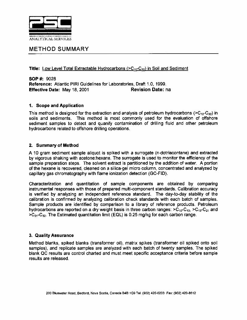

METHOD SUMMARY Title: Polycyclic Aromatic Hydrocarbons in Soils and Sediments SOP #: 7010 Reference: USEPA Method 8270C Effective Date: January, 1997 Revision Date: June, 2000 1. Scope and Application This method is applicable to the determination of polycyclic aromatic hydrocarbons (PAHs) in soils and sediments with a reporting limit of 0.05 mg/kg. The following compounds are routinely determined:
Analyte Analyte Naphthalene Benz[a]anthracene 1-Methylnaphthalene Chrysene 2-Methylnaphthalene Benzo[b]fluoranthene Acenaphthylene Benzo[k]fluoranthene Acenaphthene Benzo[a]pyrene Fluorene Perylene Phenanthrene Indeno[1,2,3-cd]pyrene Anthracene Dibenz[a,h]anthracene Fluoranthene Benzo[ghi]perylene Pyrene
Other PAHs can be analyzed by this method provided appropriate standards are available.
2. Summary of Method
A representative 5 gram portion of wet soil or sediment is weighed out and spiked with 4 deuterated surrogate PAH compounds. These compounds are used to monitor the efficiency of the sample preparation steps. The sample is extracted for 30 minutes by vigorous shaking with a mixture of 50:50 (v:v) acetone:hexane. The hexane is partitioned from the acetone by the addition of organic free water. If required, interfering compounds are removed using a silica gel solid phase extraction (SPE) clean-up procedure. The extract is analyzed by capillary gas chromatography/mass spectrometry (GC/MS) using selected ion monitoring mode.
The GC/MS system is calibrated with PAH standards of known concentration. Calibration curves are prepared by integrating the areas of target ions of the individual PAH peaks obtained during the calibration runs. Calibration accuracy is verified by analyzing an independent reference standard. The day-to-day stability of the calibration is confirmed by analyzing calibration check standards with each batch of samples. The components in the samples are identified using retention time criteria and qualifier ion ratios. After being detected, the individual peaks are integrated and quantified. The wet weight concentrations for each sample are converted to dry weight concentrations using the sample percent moisture value. The percent moisture of each sample is determined separately by gravimetric analysis. 3. Quality Assurance A method blank, spiked blanks (each individual PAH), matrix spike (each PAH spiked onto a soil sample), and a replicate sample are analyzed with each batch of twenty samples. The spiked blank QC results are control charted and must meet specific acceptance criteria before sample results are released.

METHOD SUMMARY Title: Total Sulphur in Rock, Soil and Sediment SOP #: 4075 Reference: ASTM E1915-97 / LECO Application # 203-601-222 Effective Date: August, 1998 Revision Date: August, 1998 1. Scope and Application This method is applicable for the analysis of total sulphur in homogeneous, dried rock, soil and sediment samples. The LOQ is 0.01% (dry weight) based on the combustion of a 350 mg sample. 2. Summary of Method (Combustion / IR Detector) The sample is dried at a temperature of 105C for a minimum of 1 hour. The dried sample is then ground/pulverized and sieved to –200 Mesh. A 0.2g to 0.5g aliquot of dried, homogeneous sample is combusted in a LECO induction furnace. The sulphur present in the sample is oxidized to SO2 which is swept downstream to an infra-red detection system. 3. Quality Assurance Quality control effort includes the analysis of reference materials specific to the matrix being analyzed (eg, NIST 638 for limestone and cement, RTS-1 for waste rock and tailings, STSD-3 for sediment) and duplicates.

METHOD SUMMARY Title: Total Carbon / Organic Carbon in Soils and Sediments SOP #: 4055 Reference: Total Carbon and Organic Carbon in Sludges - LECO Effective Date: January, 1995 Revision Date: July, 1997
1. Scope and Application This method is designed for the analysis of total carbon and organic carbon in soil and sediment samples by LECO EC-12 Carbon Analyzer as referenced in Application #130 from LECO Equipment Corp. The LOQ for this procedure is 0.1 %. 2. Summary of Method A known quantity of air dried and sieved sample is is introduced into the instrument with the addition of copper accelerator. An induction furnace releases all carbon in the sample as CO2 which is swept away with the sparging gas. The CO2 is then scrubbed out of the gas stream and quantified at the detector as total carbon. Organic carbon is measured by pre-treating the sample in order to remove the inorganic carbon. The sample is digested with hydrochloric acid in order to drive off all carbonates, then dried prior to the above analysis. 3. Quality Assurance A minimum of one reagent blank, one duplicate and one certified reference material (usually MESS-1) is analyzed for each set of samples. A total QC effort of 10 % should be maintained.

METHOD SUMMARY Title: Total Trace Metals in Soils and Sediments SOP #: #3010 / #4079 Reference: USEPA Method 3052 and Method 200.8 Effective Date: August, 1995 Revision Date: June, 1998 1. Scope and Application
This method is designed for the digestion and analysis of total trace metals in soil and sediment samples. Analytes and their routine LOQs are listed below:
Analyte LOQ (mg/kg) Analyte LOQ (mg/kg) Aluminum 10 Manganese 2 Antimony 2 Molybdenum 2 Arsenic 2 Nickel 2 Barium 5 Selenium 2 Beryllium 5 Silver n/a Boron n/a Strontium 5 Cadmium 0.3 Thallium 0.1 Chromium 2 Tin 2 Cobalt 1 Uranium 0.1 Copper 2 Vanadium 2 Iron 20 Zinc 2 Lead 0.5
2. Summary of Method
A 0.500 gram portion of the air-dried sieved sample is accurately weighed for analysis. An acid mixture (HClO4: HNO3: HF) is added, and the samples are slowly heated to dryness. The samples are then cooled, and HCl and HNO3 are added. After gentle warming, reagent grade water is added and the digestion cycle is completed. The samples are cooled and made to volume with reagent grade water. All samples are then diluted prior to analysis using a Sciex/Perkin Elmer Elan 5000 ICP-MS in accordance with EPA Method 200.8. 3. Quality Assurance
Reagent blanks, certified reference materials, and method spikes are prepared and analyzed in the exact same fashion as mentioned above for the samples. A minimum of one reagent blank and two different certified sediment reference materials (usually MESS-2 and BCSS-1) are prepared and analyzed with every 20 samples. Spiking of samples at a level appropriate to the matrix is performed at a frequency of 10%. Duplicate digestion and analysis of samples is also performed at a frequency of 10%.

APPENDIX H
Sediment Particle Size Method Summary

Air Quality C Environmental Sciences C Environmental Engineering C Hydrogeology C Environmental Management SystemsIntegrated Risk Management Services C Geotechnical Engineering C Materials Engineering C Mining Engineering C Petroleum Engineering
ISO 9001Newfoundland & Labrador C Nova Scotia C New Brunswick C Prince Edward Island C Quebec C Ontario C Saskatchewan C Alberta C BritishColumbia C Northwest Territories C Maine C New Hampshire C New York C Pennsylvania C Massachusetts C Trinidad C Russia C Argentina
JWEL Project No. 8206
November 13, 2002
Ms. Elizabeth DeBloisJacques Whitford Environment Limited607 Torbay RoadSt. John’s, NF A1A 4Y6
Dear Ms. DeBlois:
Re: Particle Size Analysis by Pipette MethodTerra Nova EEM 2002, Grand Banks, NF
As requested, particle size analysis by the pipette method has been conducted on the fifty-three soil samples submitted to ouroffice on September 13, 2002 for the above referenced project.
The particle size analysis has been completed in general accordance with British Standard BS 1377, Part 2 as per our ISO WorkInstruction WI 9.4.2.15. A copy of our ISO Work Instruction and our Method Summary is enclosed for reference in AppendixC.
The test results are summarized on the enclosed Tables and the individual graph reports for each sample are presented on the GrainSize Distribution Sheets in Appendix A. As per our Work Instruction, duplicate samples were also tested and the results areenclosed in Appendix B. The gravel, silt and clay portions are based on the grain sizes indicated by the Wentworth classification.(Gravel: >2.0 mm; Sand: < 2.0 mm, >0.630 :m; Silt: < 0.630 :m, > 4 :m; Clay: < 4 :m.
We trust this service has been to your satisfaction. If you have any questions or require any additional information, please contactthe undersigned at your convenience.
Yours truly,
NEWFOUNDLAND GEOSCIENCES LIMITED
Perry G. Dalton, CETMaterials Supervisor
Enclosures; Appendix A Summary Tables – Sample Test ResultsGrain Size Distribution Sheets
Appendix B Summary Table – Duplicate Test ResultsGrain Size Distribution Sheets (Duplicate Samples)
Appendix C Method SummaryISO Work Instruction Sheet
607 Torbay Road, St. John's, Newfoundland, A1A 4Y6Tel: (709) 576-1458, Fax: (709) 576-2126
World Wide Web: www.jacqueswhitford.comEmail: [email protected]
Jacques WhitfordEnvironment Limited
Consulting EngineersEnvironmental ScientistsRisk Consultants

Page: 1 of 1JACQUES WHITFORD
NEWFOUNDLAND AND LABRADOR Date Issued: April 1, 2002
Work Instruction: 9.4.2.15 Particle Size Determination by the Pipette Method
ISO 9001 Uncontrolled if Printed
1.0 PURPOSE AND SCOPE
To determine particle size distribution in a soil from gravel sizes to the clay size by the pipette method.
This work instruction is applicable to all samples of construction aggregates and soils for which grain sizedistribution determination by the pipette test is required or requested by the client.
2.0 METHOD
The pipette test will be carried out in general accordance with BS 1377, Part 2.
Testing will include duplicate analysis of samples when deemed appropriate by the Project Officer. Theresults of the duplicate analysis shall be reviewed by the Project Officer and any difference greater thandeemed acceptable by the Project Officer shall be documented.
3.0 DOCUMENTATION
The test results shall be recorded and submitted to the Project Officer on the appropriate report form. Theresults are reviewed and a computer generated report is prepared for delivery to the client. A sample reportis attached for reference.
MA101 Aggregate Mechanical Sieve AnalysisMA111 Grain Size Distribution by Pipette Method Laboratory Sheet
K:\WORDVERSIONISO\MAT\WI&SOP\9-4-2\9-4-2-15.DOC

APPENDIX I
Body Burden Methods Summaries
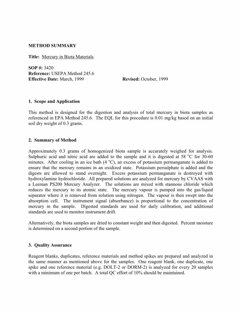
METHOD SUMMARY Title: Mercury in Biota Materials SOP #: 3420 Reference: USEPA Method 245.6 Effective Date: March, 1999 Revised: October, 1999 1. Scope and Application This method is designed for the digestion and analysis of total mercury in biota samples as referenced in EPA Method 245.6. The EQL for this procedure is 0.01 mg/kg based on an initial soil dry weight of 0.3 grams. 2. Summary of Method Approximately 0.3 grams of homogenized biota sample is accurately weighed for analysis. Sulphuric acid and nitric acid are added to the sample and it is digested at 58 oC for 30-60 minutes. After cooling in an ice bath (4 oC), an excess of potassium permanganate is added to ensure that the mercury remains in an oxidized state. Potassium persulphate is added and the digests are allowed to stand overnight. Excess potassium permanganate is destroyed with hydroxylamine hydrochloride. All prepared solutions are analyzed for mercury by CVAAS with a Leeman PS200 Mercury Analyzer. The solutions are mixed with stannous chloride which reduces the mercury to its atomic state. The mercury vapour is pumped into the gas/liquid separator where it is removed from solution using nitrogen. The vapour is then swept into the absorption cell. The instrument signal (absorbance) is proportional to the concentration of mercury in the sample. Digested standards are used for daily calibration, and additional standards are used to monitor instrument drift. Alternatively, the biota samples are dried to constant weight and then digested. Percent moisture is determined on a second portion of the sample. 3. Quality Assurance Reagent blanks, duplicates, reference materials and method spikes are prepared and analyzed in the same manner as mentioned above for the samples. One reagent blank, one duplicate, one spike and one reference material (e.g. DOLT-2 or DORM-2) is analyzed for every 20 samples with a minimum of one per batch. A total QC effort of 10% should be maintained.

METHOD SUMMARY
Title: Moisture Content
SOP #: 4003 .
Reference: Handbook of Analytical Method for Environmental Samples, Vol. 1 Effective Date: November, 1995 Revision Date: July, 1997
1. Scope and Application
This method is applicable to the determination of percent moisture in soil, sediments andbiota materials. The EQL for this method is 0.5%.
2. Summary of Method
Approximately 1 to 5 grams of homogenized sample is placed into a preweighed labeledaluminum weighing dish. The weight of the wet soil and the aluminum dish is determinedusing a top loading balance. The samples are placed in the oven at 110°C for two hours.The samples are removed from the oven, re-weighed and the percent moisture iscalculated.
3. Quality Assurance
Samples are analyzed in duplicate at a rate of 10 percent.

METHOD SUMMARY
Title: Polycyclic Aromatic Hydrocarbons in Fish and Shellfish
SOP #: 7030 Reference: Based on USEPA Method 8270AEffective Date: January 1996 Revision Date: August, 2001
1. Scope and ApplicationThis method is applicable to the determination of polycyclic aromatic hydrocarbons (PAHs) in tissuessamples with EQLs of 0.05 mg/Kg on a wet weight basis. The following compounds are routinelydetermined:
Analyte AnalyteNaphthalene Benz[a]anthracene1-Methylnaphthalene Chrysene2-Methylnaphthalene Benzo[b]fluorantheneAcenaphthylene Benzo[k]fluorantheneAcenaphthene Benzo[a]pyreneFluorene PerylenePhenanthrene Indeno[1,2,3-cd]pyreneAnthracene Dibenz[a,h]anthraceneFluoranthene Benzo[ghi]perylenePyrene
Other PAHs can be analyzed by this method provided appropriate standards are available.
2. Summary of Method
The tissue is homogenized in a blender and a 5 g portion is weighed out and spiked with 4 deuteratedsurrogate PAH compounds (these compounds represent a range of volatilities and are used to monitor theefficiency of the sample preparation steps). The sample is saponified with ethanolic KOH and thenextracted with hexane. An aliquot of the extract is removed and interfering compounds are eliminatedusing a silica gel column clean-up procedure. The extract is then solvent exchanged into isooctane andanalyzed by gas chromatography/mass spectrometry (GC/MS) using selected ion monitoring mode.
The GC/MS system is calibrated with PAH standards of known concentration. Calibration curves areprepared by integrating the areas of target ions of the individual PAH peaks obtained during the calibrationruns. Calibration accuracy is verified by analyzing an independent reference standard. The day-to-daystability of the calibration is confirmed by analyzing calibration check standards with each batch ofsamples. The components in the samples are identified using retention time criteria and qualifier ion ratios.After being detected, the individual peaks are integrated and quantified.
3. Quality Assurance A method blank, spiked blanks (each individual PAH), matrix spike (each PAH spiked onto a tissuesample), and a replicate sample are analyzed with each batch of twenty samples. The spiked blank QCresults are control charted and must meet specific acceptance criteria before sample results are released.

METHOD SUMMARY
Title: Total Extractable Hydrocarbons (>C10-C32) in Fish and Shellfish
SOP #: Draft Reference:Effective Date: September 2001 Revision Date: February, 2003
1. Scope and ApplicationThis method is designed for the extraction and analysis of petroleum hydrocarbons,including diesel range organics (>C10-C21) and lubricating oils (>C21-C32) in tissues andbiota. The EQLs are as follows: >C10-C21 (15 mg/Kg) and >C21-C32 (15 mg/Kg) and areon a wet weight basis.
2. Summary of MethodThe tissue is homogenized in blender and a 5 g portion is weighed out and spiked with asurrogate compound (n-dotriacontane). This compound ise used to monitor theefficiency of the sample preparation steps. The sample is saponified with ethanolic KOHat 600C. It is then extracted with hexane. An aliquot of the extract is removed andinterfering compounds are eliminated using a silica gel column clean-up procedure. Theextract is then solvent exchanged into isooctane and analyzed by gas chromatographywith flame ionization detection.
The GC-FID system is calibrated with multi-component standards of knownconcentration which elute in the >C10 – C32 range. A calibration curve is generated foreach carbon range (>C10 - C21 and >C21 – C32) using the response factor of thecompounds that elute in each range. Calibration accuracy is verified by analyzing anindependent reference standard. The day-to-day stability of the calibration is confirmedby analyzing calibration check standards with each batch of samples. Sample productsare identified by comparing each product to a library of reference products.
3. Quality Assurance
Method blanks (containing commercially available fish tissue), spiked blanks (transformer oilspiked on commercially available fish tissue), matrix spikes (transformer oil spiked onto tissuesamples), and replicate samples are analyzed with each batch of twenty samples. The spikedblank QC results are control charted and must meet specific acceptance criteria before sampleresults are released.

METHOD SUMMARY
Title: Trace Metals in Biota Samples
SOP #: 3010 / 4081Reference: USEPA Method 200.8Effective Date: August, 1995 Revision Date: June, 1998
1. Scope and Application
This method is designed for the digestion and analysis of trace metals in biota samples. Analytes and LOQs (wetweight basis) are as listed below:
Analyte LOQ (mg/kg) Analyte LOQ (mg/kg)Aluminum 2.5 Manganese 0.5Antimony 0.5 Molybdenum 0.5Arsenic 0.5 Nickel 0.5Barium 1.5 Selenium 0.5Beryllium 1.5 Silver 0.12Boron 1.5 Strontium 1.5Cadmium 0.08 Thallium 0.02Chromium 0.5 Tin 0.5Cobalt 0.2 Uranium 0.02Copper 0.5 Vanadium 0.5Iron 5 Zinc 0.5Lead 0.1
2. Summary of Method
A ~2.5 gram portion (depending upon sample type and estimated moisture content) of the homogenized biotasample is accurately weighed for analysis. High purity HNO3 is added to each sample, and allowed to standovernight. The samples are then slowly digested until the acid volume is reduced to less than 1 mL. AdditionalHNO3 is added and the digestion cycle is repeated. HNO3 and reagent grade water is then added to the sampleswhich are gently heated. After cooling, the samples are made to volume. The samples are then diluted prior toanalysis using a Sciex/Perkin-Elmer Elan 5000 ICP-MS in accordance to EPA Method 200.8.
3. Quality Assurance
Reagent blanks, certified reference materials, and method spikes are prepared and analyzed in the exact samefashion as mentioned above for the samples. A minimum of one reagent blank and two different biota referencematerials (usually DORM-1 and DOLT-2) are prepared and analyzed with each batch of samples. Spiking ofsamples at a level appropriate to the matrix is performed at a frequency of 10%. Duplicate digestion and analysisof samples is also performed at a frequency of 10%.