white dwarf kinematics versus mass - core · white dwarf kinematics versus mass 429 to the distance...

Mon. Not. R. Astron. Soc. 426, 427–439 (2012) doi:10.1111/j.1365-2966.2012.21394.x

White dwarf kinematics versus mass

Christopher Wegg� and E. Sterl PhinneyDepartment of Physics, Mathematics and Astronomy, MC 350-17, California Institute of Technology, Pasadena, CA 91125, USA

Accepted 2012 May 24. Received 2012 May 24; in original form 2011 July 4

ABSTRACTWe investigated the relationship between the kinematics and mass of young (<3 × 108 yr)white dwarfs using proper motions. Our sample is taken from the colour-selected catalogues ofthe Sloan Digital Sky Survey and the Palomar–Green Survey, both of which have spectroscopictemperature and gravity determinations. We find that the dispersion decreases with increasingwhite dwarf mass. This can be explained as a result of less scattering by objects in the Galacticdisc during the shorter lifetime of their more massive progenitors. A direct result of this isthat white dwarfs with high mass have a reduced scale height, and hence their local densityis enhanced over their less massive counterparts. In addition, we have investigated whetherthe kinematics of the highest mass white dwarfs (>0.95 M�) are consistent with the expectedrelative contributions of single star evolution and mergers. We find that the kinematics areconsistent with the majority of high-mass white dwarfs being formed through single starevolution.

Key words: white dwarfs – Galaxy: kinematics and dynamics.

1 IN T RO D U C T I O N

Despite the significant work on both the kinematics and mass distri-bution of white dwarfs (WDs), very little work has addressed theirconnection.

The kinematics of galactic WDs have been studied on numerousoccasions with several motivations. They have proven useful in at-tempts to unravel the evolutionary history and progenitors of thevarious classes of WDs (Sion et al. 1988; Anselowitz et al. 1999).Interest in WD kinematics was also prompted by the suggestionthat halo WDs could provide a significant contribution to Galacticdark matter (Oppenheimer et al. 2001; Reid 2005). This effort hasconcentrated on the identification of halo WDs and estimating theresultant density, which now appears to be a small contribution tothe Galactic dark matter budget (Pauli et al. 2006). Moreover, themass distribution of the most common hydrogen-rich (DA) WDshas also been extensively investigated, particularly for WDs withT � 10 000 K which are hot enough for their masses to be de-duced spectroscopically from fits to their Balmer lines (Vennes1999; Liebert et al. 2005; Kepler et al. 2007). The mass distributionshows a peak at 0.6 M� due to the relative abundance of their lowermass progenitors with a tail extending to higher masses formedfrom more massive progenitors.

The connection between the galactic kinematics of a group ofthin disc objects and their progenitors is largely due to the processof kinematic disc ‘heating’ (Wielen 1977; Nordstrom et al. 2004).The hot WDs with short cooling ages we observe in the galactic

�E-mail: [email protected]

neighbourhood today are formed from a wide range of progenitormasses (∼0.8–8 M�) and hence have a wide range in age. We there-fore expect high-mass disc WDs to have a low velocity dispersionin comparison to low-mass disc WDs whose progenitors formedearlier. This connection was suggested in Guseinov, Novruzova &Rustamov (1983) who performed an analysis suggesting that WDswith larger masses have smaller dispersions; however, this was rein-vestigated by Sion et al. (1988) with a larger sample of 78 DA WDswhere no evidence for any correlation was found. This paper read-dresses the connection between mass and kinematics with a greatlyincreased sample size.

The outline of the paper is as follows. In Section 2, we discuss thesample selection and the calculation of distances and proper mo-tions. In Section 3, we discuss how we estimate the kinematics of thesample without radial velocity information. We use two methods,that of Dehnen & Binney (1998) (Section 3.1) and a Markov ChainMonte Carlo (MCMC), where we marginalize over the unknownradial velocity (Section 3.2). In Section 4, we analyse whether thekinematics are consistent with single star evolution (SSE) both viaanalytic methods (Section 4.1) and simulations (Section 4.2). InSection 5, we analyse whether the highest mass WDs are largelyformed through SSE or are the product of the merger of two lowermass WDs. Finally, we discuss the implications of our findings onthe scale height of WDs in Section 6.

For the reader in a hurry, the primary result of this paper, therelationship between the mass of young WDs and their velocitydispersion, is shown in Fig. 3 and discussed in Section 3. Theimplied scale heights, the second key result, are then discussed inSection 6. These results have been checked using a Monte Carlosimulation of the formation and observation of an ensemble of WDs,

C© 2012 The AuthorsMonthly Notices of the Royal Astronomical Society C© 2012 RAS

428 C. Wegg and E. S. Phinney

Table 1. Summary of the sample.

PG SDSS

Number of DA white dwarfs with 299 6926good photometry not known to be binariesof these number with signal-to-noise >10 299 3125of these number with 13 000 K < Teff < 40 000 K 215 1555of these number with age <3 × 108 yr 211 1491

Distance source:Liebert et al. (2005) 79 0SDSS photometry 132 1491of these numbers rejected with χ2 > 5 0 48

Proper motion source:Munn et al. (2008) 153 1443PPMXL 54 0Manual measurement from POSS I/II 4 0

which is described by flowcharts in Figs 6–8: in Fig. 6 the processof choosing stars is described, in Fig. 7 the process of placing themin the disc is described and in Fig. 8 the process of determining theobservability of the simulated WD is described.

2 SA MPLE

We investigate only hydrogen atmosphere (DA) WDs due to therelative simplicity of their spectra and the resultant security of thespectroscopic masses. The sample of DA WDs is taken from twosources, the Palomar–Green (PG) white dwarf survey (Liebert et al.2005) and the Sloan Digital Sky Survey (SDSS) DR4 white dwarfsurvey (Eisenstein et al. 2006). The SDSS sample is much largerthan the PG sample. The PG sample is included as a demonstrationthat the results are secure, and not a result of systematics in theSDSS, such as the complex selection of targets. For clarity, we firstdiscuss which types of WDs we select, then discuss how the SDSSis dealt with, and finally how the PG survey was dealt with. Thesample and its selection are summarized in Table 1.

2.1 Selected WDs

Both PG and SDSS are colour selected, eliminating the kinematicbiases inherent in proper motion-based surveys, and contain spec-troscopic determinations of surface gravity, log g, and effective tem-perature, Teff , obtained by fitting the profile of the Balmer lines. Werestrict the sample to objects whose fitted Teff was between 13 000and 40 000 K, since log g appears to be systematically overestimatedat low temperatures and Teff overestimated at higher temperatures(Eisenstein et al. 2006).

The fitted log g and Teff are converted to masses and ages us-ing the carbon core WD cooling models of Fontaine, Brassard &Bergeron (2001) below 30 000 K and Wood (1995) with thick hy-drogen layers of fractional mass 10−4 above 30 000 K.1 WDs withinferred masses less than 0.47 M� are instead assumed to have he-lium cores whose masses and ages are calculated from the modelsof Serenelli et al. (2001). Only objects with cooling ages below3 × 108 yr are included in the sample to avoid significant kinematicheating after WD formation. The requirements of cooling age below3 × 108 yr and Teff above 13 000 K are competing. Above 0.60 M�,

1 Available from http://www.astro.umontreal.ca/bergeron/CoolingModels/,uses results from Holberg & Bergeron (2006), Kowalski & Saumon (2006),Tremblay, Bergeron & Gianninas (2011) and Bergeron et al. (2011).

the WDs cool more slowly and thus the age limit is used, while be-low 0.60 M� the temperature limit is used.

WDs previously discussed in the literature as known members ofbinaries were removed from the samples.

2.2 SDSS (Eisenstein et al. 2006)

Many of the SDSS spectra have low signal-to-noise ratios and hencelarge errors on their fitted log g and Teff . To ensure accurate massesand photometric distances, only objects whose spectra had a signal-to-noise ratio larger than 10 are included. The grid of model at-mospheres fitted in the SDSS catalogue extends only to log g = 9,and thus, for objects at this limit, the refitted log g and Teff given inKepler et al. (2007) were used.

Photometric distances to the WDs in the SDSS are calculated byminimizing

χ2 =∑

i=(u,g,r,i,z)

(mi − [Mi(log g, Teff )

+ Agai + 5 log d − 5])2/σ 2i , (1)

where mi and σ i are the five-band SDSS photometry and their errors,Mi are the model absolute magnitudes, Agai is the reddening and dthe distance in parsecs.The error σ i is the quoted photometric errorin SDSS each band added in quadrature to a systematic error of(u, g, r, i, z) = (0.015, 0.007, 0.007, 0.007, 0.01) (Kleinman et al.2004). Model absolute magnitudes are taken from the atmosphericmodels provided by Bergeron (see footnote 1). Agai is the product ofRV = 3.1 extinction in each band of (au, ag, ar, ai, az) = (1.36, 1.00,0.73, 0.55, 0.39) and the overall extinction Ag, which is constrainedto lie between zero and the value of the galactic extinction map ofSchlegel, Finkbeiner & Davis (1998) at the position of the objectconsidered.

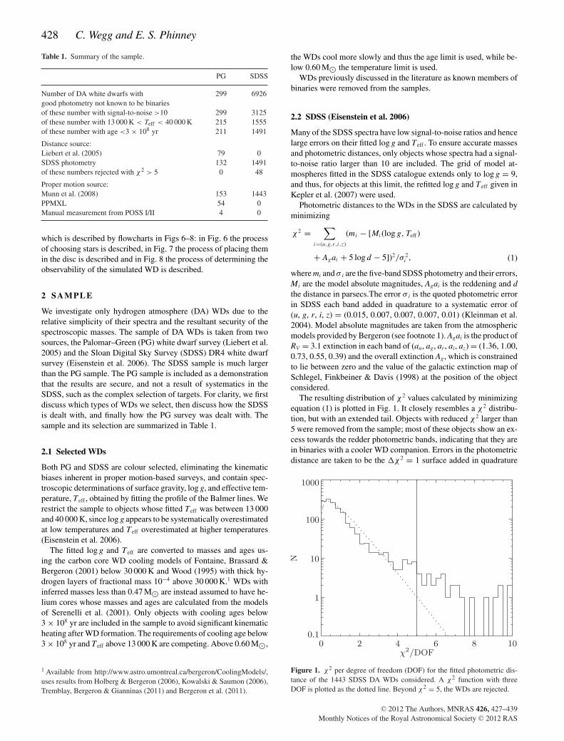
The resulting distribution of χ2 values calculated by minimizingequation (1) is plotted in Fig. 1. It closely resembles a χ2 distribu-tion, but with an extended tail. Objects with reduced χ2 larger than5 were removed from the sample; most of these objects show an ex-cess towards the redder photometric bands, indicating that they arein binaries with a cooler WD companion. Errors in the photometricdistance are taken to be the �χ2 = 1 surface added in quadrature

Figure 1. χ2 per degree of freedom (DOF) for the fitted photometric dis-tance of the 1443 SDSS DA WDs considered. A χ2 function with threeDOF is plotted as the dotted line. Beyond χ2 = 5, the WDs are rejected.

C© 2012 The Authors, MNRAS 426, 427–439Monthly Notices of the Royal Astronomical Society C© 2012 RAS

White dwarf kinematics versus mass 429

to the distance errors introduced though the uncertainty in log g andTeff .

Proper motions for the SDSS sample are taken from the catalogueof Munn et al. (2008). These proper motions are calculated fromthe USNO-B1.0 plate positions re-calibrated using nearby galaxiestogether with the SDSS position so that the proper motions are moreaccurate and absolute. By measuring the proper motions of quasars,Munn et al. (2004) estimate that the 1σ error is 5.6 mas yr−1.

2.3 PG survey

For 132 stars in the PG survey, SDSS photometry was available andthe same method was used as for SDSS stars. For the remainingobjects, the PG catalogue photometric distances were used. Thesewere estimated in Liebert et al. (2005) from comparison of theV-band magnitude with the predicted MV from the same modelsof Holberg & Bergeron (2006). Comparison of the stellar distancesgiven by the two methods gives a standard deviation of 7 per cent.The majority of this error is expected to be in the PG survey distancesand hence a conservative 10 per cent error was applied to these.

Proper motions for PG WDs that appear in the SDSS are takenfrom the catalogue of Munn et al. (2008). For the remaining objects,the PPMXL proper motion was used where available, which has atypical 1σ error of ∼8 mas yr−1(Roeser, Demleitner & Schilbach2010).

Finally, four objects in the PG sample have no reliable PPMXLproper motion, primarily due to a spurious matching of objects be-tween epochs. For these, the proper motion was calculated directlybetween the scanned Palomar Observatory Sky Survey (POSS)-Iand POSS-II plates. The proper motion was measured relative tonearby faint stars of similar magnitude corrected for galactic ro-tation (see Section 3.1). Typical errors estimated from the propermotions of stars of similar magnitude to be 11 mas yr−1. We em-phasize that only 4 of 1491 WDs use this method, and none havemass above 0.95 M� analysed in more detail in Section 5.

2.4 Final sample

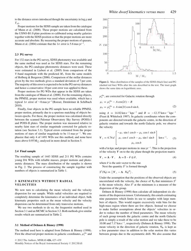
The resulting sample of 1443 SDSS and 211 PG WDs containsyoung DA WDs with reliable masses, proper motions and photo-metric distances. The mass distribution of the samples is shownin Fig. 2. The process of constructing the sample together withnumbers of objects is summarized in Table 1.

3 K I N E M AT I C S W I T H O U T R A D I A LV E L O C I T I E S

We now turn to calculating the mean velocity and the velocitydispersion for our sample. While radial velocities are required tocompletely determine the kinematics of an individual object, bulkkinematic properties such as the mean velocity and the velocitydispersion can be determined from only transverse motions.

We use two methods to do so, the frequentist method used inSection 3.1 and an MCMC in Section 3.2. Both methods give similarresults which are summarized in Table 2.

3.1 Method of Dehnen & Binney (1998)

The method used here is adapted from Dehnen & Binney (1998).First the observed proper motions in galactic coordinates, μobs

� and

Figure 2. Mass distribution of the samples of the SDSS (black line) and PG(dashed red line) WDs after the cuts described in the text. The inset graphshows the same data on logarithmic axes.

μobsb , are corrected for Galactic rotation through

μ� = μobs� − A cos(2�) − B

μb = μobsb + A sin(2�) cos b sin b, (2)

using A = 14.82 km s−1 kpc−1 and B = −12.37 km s−1 kpc−1

(Feast & Whitelock 1997). In galactic coordinates where the com-ponents are directed towards the galactic centre, in the direction ofgalactic rotation and towards the north Galactic pole, we observethe velocity

V ⊥ = 4.74 d

⎡⎢⎢⎣

−μ� sin � cos b − μb cos � sin b

μ� cos � cos b − μb sin � sin b

μb cos b

⎤⎥⎥⎦ km s−1, (3)

with d in kpc and proper motions in mas yr−1. This is the projectionof the velocity V on to the sky plane though the projection matrix

V ⊥ = A · V , A = I − r ⊗ r, (4)

where r is the unit vector to the star.Next the quantity S2 is formed through

S2(V0) ≡ ⟨|V ⊥ − A · V0|2⟩. (5)

Under the assumption that the positions of the observed objects areuncorrelated with the velocity, the choice of V0 that minimizes S2

is the mean velocity. Also S2 at the minimum is a measure of thedispersion of the group.

Dehnen & Binney (1998) then calculate all independent six ele-ments of the dispersion tensor. Unfortunately, this entails estimatingnine parameters which limits its use to samples with large num-bers of objects. This would require excessively wide bins for thehigh-mass region where there are few objects. Instead we chooseto make further assumptions about the objects’ velocities in or-der to reduce the number of fitted parameters. The mean velocityof each group towards the galactic centre and the north Galacticpole is simply a result of the solar motion and we take these to be10.00 and 7.17 km s−1, respectively (Dehnen & Binney 1998). Themean velocity in the direction of galactic rotation, V0, is kept asa free parameter since in addition to the solar motion this variesbetween groups due to the asymmetric drift. We also assume that



Table 2. Kinematic fitting results from the PG and SDSS samples described in Section 2 using the methods of Sections 3.1 and 3.2. Mlow and Mhigh

are in units of M�, while σ 1 and V are in km s−1. N is the number of WDs in each mass bin.

PG SDSS

Mlow Mhigh NDehnen & Binney

(1998) MCMC NDehnen & Binney

(1998) MCMCσ 1 V σ 1 V σ 1 V σ 1 V

0.30 0.40 5 47 ± 12 22 ± 13 48 ± 10 18 ± 12 70 53 ± 3 33 ± 4 40 ± 3 34 ± 40.40 0.47 20 49 ± 6 27 ± 7 49 ± 7 28 ± 6 62 68 ± 4 38 ± 6 70 ± 6 38 ± 60.47 0.55 35 47 ± 4 18 ± 6 51 ± 4 17 ± 4 333 56 ± 1 34 ± 2 57 ± 2 34 ± 20.55 0.60 53 37 ± 2 17 ± 3 40 ± 3 18 ± 3 482 46 ± 1 20 ± 1 45 ± 1 21 ± 10.60 0.65 51 37 ± 2 16 ± 3 34 ± 2 15 ± 2 239 33 ± 1 20 ± 1 31 ± 1 20 ± 10.65 0.75 23 33 ± 3 15 ± 4 34 ± 4 14 ± 5 91 26 ± 1 16 ± 2 28 ± 1 15 ± 10.75 0.85 9 16 ± 2 11 ± 4 17 ± 3 11 ± 4 30 16 ± 1 11 ± 2 19 ± 2 11 ± 20.85 0.95 10 12 ± 2 15 ± 2 12 ± 2 13 ± 2 28 18 ± 1 12 ± 2 19 ± 2 11 ± 20.95 1.44 5 22 ± 5 14 ± 7 24 ± 6 12 ± 6 9 19 ± 3 9 ± 5 24 ± 5 9 ± 6

the dispersion tensor takes the form

σ = σ1diag

(1,

1

1.4,

1

2.2

), (6)

which is accurate for main sequence stars in the solar neighbourhood(Dehnen & Binney 1998). This reduces the number of parametersfor each group to the asymmetric drift V0 and the normalization ofthe dispersion tensor σ 1.

V0 is calculated by minimizing equation (5), and then σ 1 is esti-mated through a Monte Carlo simulation. Since S2 is a measure ofdispersion, an initial estimate of σ 2

1 is taken to be S2, and a set ofsimulations is performed where a new velocity is chosen for eachWD at its position in the sky from the isothermal distribution withthe assumed dispersion tensor and the calculated mean velocity. Theerror in tangential velocity, assumed to be Gaussian, is added to this.The set of simulations produces a distribution of S2 values, and σ 2

1

is iterated until the mean S2 corresponds to the value calculatedfrom observations. S2 is almost proportional to σ 2

1 when errors intangential velocity are neglected and so the error in σ 2

1 is estimatedfrom the distribution of S2 scaled by this proportionality constant.

3.2 MCMC estimate

In addition, an MCMC likelihood-based estimate of the kinematicparameters was obtained. We use uninformative flat priors for thefitted parameters.

We denote the probability that the velocity of the ith object wasV to be P (V |Di , σ i) where Di = (l, b, d, μ�, μb) is the data forthe ith object together with the corresponding errors σ i . μ� andμb are the values corrected for galactic rotation by equation (2).Under the assumption that positions are uncorrelated with velocity,the distribution function is a function only of velocity: f (V ). Inaddition, in what follows we do not consider the positions, butinstead focus on the kinematics through the velocity V . Underthese assumptions, the overall likelihood for a set of observationsof a group of WDs is

L =∏

i

∫dVf (V )P (V |Di , σ i) (7)

⇒ logL =∑

i

log∫

dVf (V )P (V |Di , σ i) (8)

≡∑

i

logLi . (9)

In calculating the likelihoods,Li , we assume a Schwarzschild distri-bution function, and a normally distributed error in proper motion.The unknown radial velocity is integrated over analytically. Explicitexpressions for Li are given in Appendix A.

Again, the dispersion tensor and mean were constrained to re-duce the number of parameters. We use flat priors on the dispersionand asymmetric drift. The expression for the likelihood was used tocalculate the maximum likelihood estimate of the dispersion tensor,while errors were estimated from an MCMC using Metropolis–Hastings sampling. When the constraints on the dispersion tensorand mean velocity were relaxed this did not substantially alter theresults, aside from the larger errors, particularly in the underpopu-lated bins due to the reduced degrees of freedom. In particular, theresults are insensitive to allowing vertex deviation.

The fitting results for the SDSS and PG samples are summarizedin Table 2 and plotted in Fig. 3. In addition, in Fig. 4 the rawtransverse velocities measured from the proper motions for threegroups of WDs are shown. The lowest mass WDs, M < 0.45 M�,are expected to be predominantly formed through binary evolutionand have a binary WD partner. This potentially introduces errorsinto their photometric distances and so we do not consider thembeyond simply stating the fitting results in Table 2.

4 EXPECTATI ONS FRO M SSE

4.1 Analytic

In this section, we describe the reasons for the relationshipbe-tween WD mass and dispersion within a simple analytic model,before moving on to the more complex Monte Carlo simulations ofSection 4.2.

Within the framework of SSE, an ensemble of WDs with thesame mass would be expected to have a dispersion σ (tTOT), whereσ (t) is the disc-heating relation, and tTOT is the total age of the WDincluding its precursor lifetime (i.e. total pre-WD stellar lifetime).Here, tTOT will be given by tTOT = tWD + tSSE(Mi(MWD)) wheretWD is the cooling age of the WD and tSSE(Mi(MWD)) is the totalprecursor lifetime, which is a function of the WD mass through theinitial–final mass relation (IFMR) Mi(Mf ). Two components of thisprediction are particularly uncertain: the disc-heating relation andthe IFMR. We discuss these now.

The best constraints on the IFMR come from open clusters. Spec-troscopic fits of the masses of WDs give the final mass. The ini-tial mass is estimated using isochrone fitting to the main-sequence



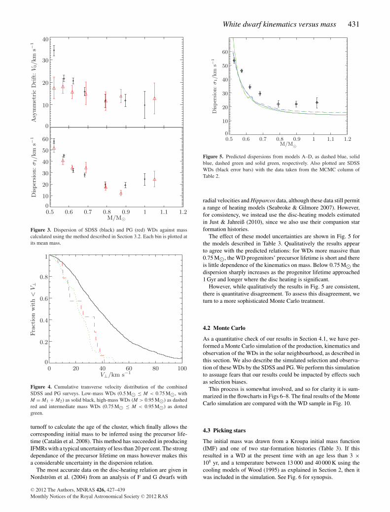
Figure 3. Dispersion of SDSS (black) and PG (red) WDs against masscalculated using the method described in Section 3.2. Each bin is plotted atits mean mass.

Figure 4. Cumulative transverse velocity distribution of the combinedSDSS and PG surveys. Low-mass WDs (0.5 M� ≤ M < 0.75 M�, withM = M1 + M2) as solid black, high-mass WDs (M > 0.95 M�) as dashedred and intermediate mass WDs (0.75 M� ≤ M < 0.95 M�) as dottedgreen.

turnoff to calculate the age of the cluster, which finally allows thecorresponding initial mass to be inferred using the precursor life-time (Catalan et al. 2008). This method has succeeded in producingIFMRs with a typical uncertainty of less than 20 per cent. The strongdependance of the precursor lifetime on mass however makes thisa considerable uncertainty in the dispersion relation.

The most accurate data on the disc-heating relation are given inNordstrom et al. (2004) from an analysis of F and G dwarfs with

Figure 5. Predicted dispersions from models A–D, as dashed blue, solidblue, dashed green and solid green, respectively. Also plotted are SDSSWDs (black error bars) with the data taken from the MCMC column ofTable 2.

radial velocities and Hipparcos data, although these data still permita range of heating models (Seabroke & Gilmore 2007). However,for consistency, we instead use the disc-heating models estimatedin Just & Jahreiß (2010), since we also use their companion starformation histories.

The effect of these model uncertainties are shown in Fig. 5 forthe models described in Table 3. Qualitatively the results appearto agree with the predicted relations: for WDs more massive than0.75 M�, the WD progenitors’ precursor lifetime is short and thereis little dependence of the kinematics on mass. Below 0.75 M� thedispersion sharply increases as the progenitor lifetime approached1 Gyr and longer where the disc heating is significant.

However, while qualitatively the results in Fig. 5 are consistent,there is quantitative disagreement. To assess this disagreement, weturn to a more sophisticated Monte Carlo treatment.

4.2 Monte Carlo

As a quantitative check of our results in Section 4.1, we have per-formed a Monte Carlo simulation of the production, kinematics andobservation of the WDs in the solar neighbourhood, as described inthis section. We also describe the simulated selection and observa-tion of these WDs by the SDSS and PG. We perform this simulationto assuage fears that our results could be impacted by effects suchas selection biases.

This process is somewhat involved, and so for clarity it is sum-marized in the flowcharts in Figs 6–8. The final results of the MonteCarlo simulation are compared with the WD sample in Fig. 10.

4.3 Picking stars

The initial mass was drawn from a Kroupa initial mass function(IMF) and one of two star-formation histories (Table 3). If thisresulted in a WD at the present time with an age less than 3 ×108 yr, and a temperature between 13 000 and 40 000 K using thecooling models of Wood (1995) as explained in Section 2, then itwas included in the simulation. See Fig. 6 for synopsis.



Table 3. Model input parameters for the models of SSE.

Model σ (t) ( km s−1) Mi(MWD) (M�) tSSE(Mi) (Gyr) SFR(t)a

A 66(

0.5+t/Gyr0.5+12

)1/2 bFrom Hurley, Pols & Tout (2000), solar metallicity 3.25b

B 62(

0.32+t/Gyr0.32+10

)1/2 c

From Hurley et al. (2000), solar metallicity 7.68 exp (−t/8 Gyr)c

C 66(

0.5+t/Gyr0.5+12

)1/2 bFrom Catalan et al. (2008) From Girardi et al. (2000)b 3.25b

D 62(

0.32+t/Gyr0.32+12

)1/2 c

From Catalan et al. (2008) From Girardi et al. (2000)c 7.68 exp (−t/8 Gyr)c

aIn units of M� pc−2 Gyr−1. Not used in the analytic SSE simulation of Section 4.1. Star formation rate (SFR).bJust & Jahreiß (2010) model C. Disc age 12 Gyr. Girardi et al. (2000) models use metal enrichment from Just & Jahreiß (2010) model C.cJust & Jahreiß (2010) model D. Disc age 10 Gyr. Girardi et al. (2000) models use metal enrichment from Just & Jahreiß (2010) model D.

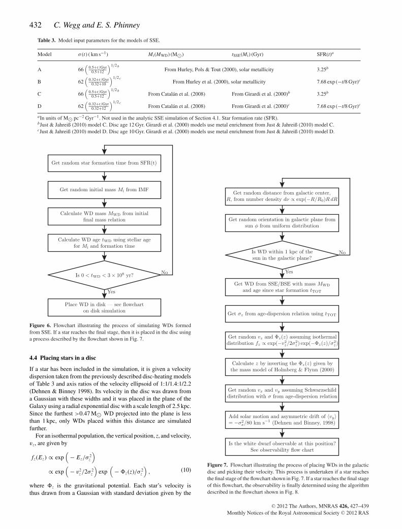
Figure 6. Flowchart illustrating the process of simulating WDs formedfrom SSE. If a star reaches the final stage, then it is placed in the disc usinga process described by the flowchart shown in Fig. 7.

4.4 Placing stars in a disc

If a star has been included in the simulation, it is given a velocitydispersion taken from the previously described disc-heating modelsof Table 3 and axis ratios of the velocity ellipsoid of 1:1/1.4:1/2.2(Dehnen & Binney 1998). Its velocity in the disc was drawn froma Gaussian with these widths and it was placed in the plane of theGalaxy using a radial exponential disc with a scale length of 2.5 kpc.Since the furthest >0.47 M� WD projected into the plane is lessthan 1 kpc, only WDs placed within this distance are simulatedfurther.

For an isothermal population, the vertical position, z, and velocity,vz, are given by

fz(Ez) ∝ exp(

− Ez/σ2z

)∝ exp

(− v2

z /2σ 2z

)exp

(− �z(z)/σ 2

z

), (10)

where �z is the gravitational potential. Each star’s velocity isthus drawn from a Gaussian with standard deviation given by the

Figure 7. Flowchart illustrating the process of placing WDs in the galacticdisc and picking their velocity. This process is undertaken if a star reachesthe final stage of the flowchart shown in Fig. 7. If a star reaches the final stageof this flowchart, the observability is finally determined using the algorithmdescribed in the flowchart shown in Fig. 8.



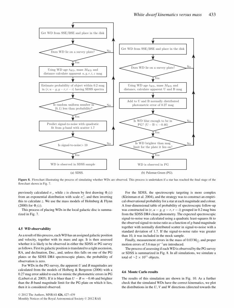
Figure 8. Flowchart illustrating the process of simulating whether WDs are observed. This process is undertaken if a star has reached the final stage of theflowchart shown in Fig. 7.

previously calculated σ z, while z is chosen by first drawing �z(z)from an exponential distribution with scale σ 2

z , and then invertingthis to calculate z. We use the mass models of Holmberg & Flynn(2000) for �z(z).

This process of placing WDs in the local galactic disc is summa-rized in Fig. 7.

4.5 WD observability

As a result of this process, each WD has an assigned galactic positionand velocity, together with its mass and age. It is then assessedwhether it is likely to be observed in either the SDSS or PG surveyas follows. First its galactic position is translated to a right ascension,RA, and declination, Dec., and, unless this falls on one of the PGplates or the SDSS DR4 spectroscopic plates, the probability ofobservation is zero.

For WDs in the PG survey, the apparent U and B magnitudes arecalculated from the models of Holberg & Bergeron (2006) with a0.27 mag error added to each to mimic the photometric errors in PG(Liebert et al. 2005). If it is bluer than U − B = −0.46 and brighterthan the B-band magnitude limit for the PG plate on which it lies,then it is considered observed.

For the SDSS, the spectroscopic targeting is more complex(Kleinman et al. 2004), and the strategy was to construct an empiri-cal observational probability for a star at each magnitude and colour.A four-dimensional table of probability of spectroscopic follow-upwas constructed in (r, u − g, g − r, r − i) grouped in 0.2 mag binsfrom the SDSS DR4 clean photometry. The expected spectroscopicsignal-to-noise was calculated using a quadratic least-squares fit tothe observed signal-to-noise ratio as a function of g-band magnitudetogether with normally distributed scatter in signal-to-noise with astandard deviation of 1.7. If the signal-to-noise ratio was greaterthan 10, it was included in the mock sample.

Finally, measurement errors in the mass of 0.03 M� and propermotion errors of 5.6 mas yr−1are introduced.

The process of assessing if each WD is observed by the PG surveyor SDSS is summarized in Fig. 8. In all simulations, we simulate atotal of ∼2 × 1011 objects.

4.6 Monte Carlo results

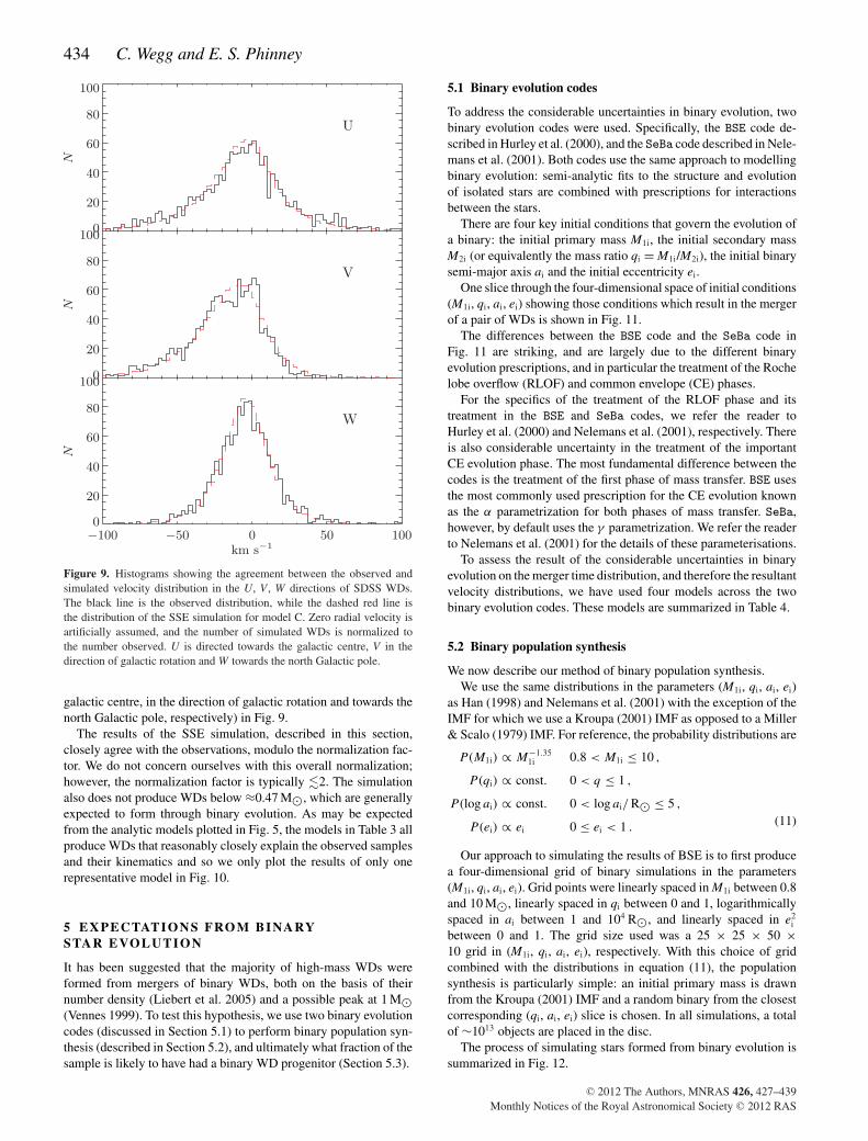
The results of this simulation are shown in Fig. 10. As a furthercheck that the simulated WDs have the correct kinematics, we plotthe distributions in the U, V and W directions (directed towards the



Figure 9. Histograms showing the agreement between the observed andsimulated velocity distribution in the U, V , W directions of SDSS WDs.The black line is the observed distribution, while the dashed red line isthe distribution of the SSE simulation for model C. Zero radial velocity isartificially assumed, and the number of simulated WDs is normalized tothe number observed. U is directed towards the galactic centre, V in thedirection of galactic rotation and W towards the north Galactic pole.

galactic centre, in the direction of galactic rotation and towards thenorth Galactic pole, respectively) in Fig. 9.

The results of the SSE simulation, described in this section,closely agree with the observations, modulo the normalization fac-tor. We do not concern ourselves with this overall normalization;however, the normalization factor is typically �2. The simulationalso does not produce WDs below ≈0.47 M�, which are generallyexpected to form through binary evolution. As may be expectedfrom the analytic models plotted in Fig. 5, the models in Table 3 allproduce WDs that reasonably closely explain the observed samplesand their kinematics and so we only plot the results of only onerepresentative model in Fig. 10.

5 EX P E C TAT I O N S FRO M BI NA RYSTAR EVOLUTION

It has been suggested that the majority of high-mass WDs wereformed from mergers of binary WDs, both on the basis of theirnumber density (Liebert et al. 2005) and a possible peak at 1 M�(Vennes 1999). To test this hypothesis, we use two binary evolutioncodes (discussed in Section 5.1) to perform binary population syn-thesis (described in Section 5.2), and ultimately what fraction of thesample is likely to have had a binary WD progenitor (Section 5.3).

5.1 Binary evolution codes

To address the considerable uncertainties in binary evolution, twobinary evolution codes were used. Specifically, the BSE code de-scribed in Hurley et al. (2000), and the SeBa code described in Nele-mans et al. (2001). Both codes use the same approach to modellingbinary evolution: semi-analytic fits to the structure and evolutionof isolated stars are combined with prescriptions for interactionsbetween the stars.

There are four key initial conditions that govern the evolution ofa binary: the initial primary mass M1i, the initial secondary massM2i (or equivalently the mass ratio qi = M1i/M2i), the initial binarysemi-major axis ai and the initial eccentricity ei.

One slice through the four-dimensional space of initial conditions(M1i, qi, ai, ei) showing those conditions which result in the mergerof a pair of WDs is shown in Fig. 11.

The differences between the BSE code and the SeBa code inFig. 11 are striking, and are largely due to the different binaryevolution prescriptions, and in particular the treatment of the Rochelobe overflow (RLOF) and common envelope (CE) phases.

For the specifics of the treatment of the RLOF phase and itstreatment in the BSE and SeBa codes, we refer the reader toHurley et al. (2000) and Nelemans et al. (2001), respectively. Thereis also considerable uncertainty in the treatment of the importantCE evolution phase. The most fundamental difference between thecodes is the treatment of the first phase of mass transfer. BSE usesthe most commonly used prescription for the CE evolution knownas the α parametrization for both phases of mass transfer. SeBa,however, by default uses the γ parametrization. We refer the readerto Nelemans et al. (2001) for the details of these parameterisations.

To assess the result of the considerable uncertainties in binaryevolution on the merger time distribution, and therefore the resultantvelocity distributions, we have used four models across the twobinary evolution codes. These models are summarized in Table 4.

5.2 Binary population synthesis

We now describe our method of binary population synthesis.We use the same distributions in the parameters (M1i, qi, ai, ei)

as Han (1998) and Nelemans et al. (2001) with the exception of theIMF for which we use a Kroupa (2001) IMF as opposed to a Miller& Scalo (1979) IMF. For reference, the probability distributions are

P (M1i) ∝ M−1.351i 0.8 < M1i ≤ 10 ,

P (qi) ∝ const. 0 < q ≤ 1 ,

P (log ai) ∝ const. 0 < log ai/ R� ≤ 5 ,

P (ei) ∝ ei 0 ≤ ei < 1 . (11)

Our approach to simulating the results of BSE is to first producea four-dimensional grid of binary simulations in the parameters(M1i, qi, ai, ei). Grid points were linearly spaced in M1i between 0.8and 10 M�, linearly spaced in qi between 0 and 1, logarithmicallyspaced in ai between 1 and 104 R�, and linearly spaced in e2

i

between 0 and 1. The grid size used was a 25 × 25 × 50 ×10 grid in (M1i, qi, ai, ei), respectively. With this choice of gridcombined with the distributions in equation (11), the populationsynthesis is particularly simple: an initial primary mass is drawnfrom the Kroupa (2001) IMF and a random binary from the closestcorresponding (qi, ai, ei) slice is chosen. In all simulations, a totalof ∼1013 objects are placed in the disc.

The process of simulating stars formed from binary evolution issummarized in Fig. 12.



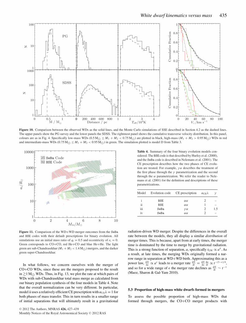
Figure 10. Comparison between the observed WDs as the solid lines, and the Monte Carlo simulations of SSE described in Section 4.2 as the dashed lines.The upper panels show the PG survey and the lower panels the SDSS. The rightmost panel shows the cumulative transverse velocity distribution. In this panel,colours are as in Fig. 4. Specifically low-mass WDs (0.5 M� ≤ M1 + M2 < 0.75 M�) are plotted in black, high-mass (M1 + M2 > 0.95 M�) WDs in redand intermediate-mass WDs (0.75 M� ≤ M1 + M2 < 0.95 M�) in green. The simulation plotted is model D from Table 3.

Figure 11. Comparison of the WD+WD merger outcomes from the SeBaand BSE codes with their default prescriptions for binary evolution. Allsimulations use an initial mass ratio of qi = 0.5 and eccentricity of ei = 0.Green corresponds to CO+CO, red He+CO and blue He+He. The lightgreen are sub-Chandrasekhar (M1 + M2 < 1.4 M�) mergers, and the darkergreen super-Chandrasekhar.

In what follows, we concern ourselves with the merger ofCO+CO WDs, since these are the mergers proposed to the resultin �1 M� WDs. Thus, in Fig. 13, we plot the rate at which pairs ofWDs with sub-Chandrasekhar total mass merge as calculated fromour binary population synthesis of the four models in Table 4. Notethat the overall normalization can be very different. In particular,model ii uses a relatively efficient CE prescription with αCEλ = 1 forboth phases of mass transfer. This in turn results in a smaller rangeof initial separations that will ultimately result in a gravitational

Table 4. Summary of the four binary evolution models con-sidered. The BSE code is that described by Hurley et al. (2000),and the SeBa code is described in Nelemans et al. (2001). TheCE prescription describes how the two phases of CE evolu-tion are treated. For example, γα describes the treatment ofthe first phase through the γ parametrization and the secondthrough the α parametrization. We refer the reader to Nele-mans et al. (2001) for the definition and descriptions of theseparametrizations.

Model Evolution code CE prescription αCEλ γ

i BSE αα 2 –ii BSE αα 1 –iii SeBa γα 2 1.5iv SeBa αα 2 –

radiation-driven WD merger. Despite the differences in the overallrate between the models, they all display a similar distribution ofmerger times. This is because, apart from at early times, the mergertime is dominated by the time to merge by gravitational radiation.This is a strong function of separation, a, specifically tGW ∝ a4. Asa result, at late times, the merging WDs originally formed a nar-row range in separation at WD+WD birth. Approximating this as apower law, dN

da∝ aε leads to a merger rate dN

dt= dN

dadadt

∝ t−(3−ε)/4,and so for a wide range of ε the merger rate declines as dN

dt∼ t−1

(Maoz, Sharon & Gal-Yam 2010).

5.3 Proportion of high-mass white dwarfs formed in mergers

To assess the possible proportion of high-mass WDs thatformed through mergers, the CO+CO merger products with



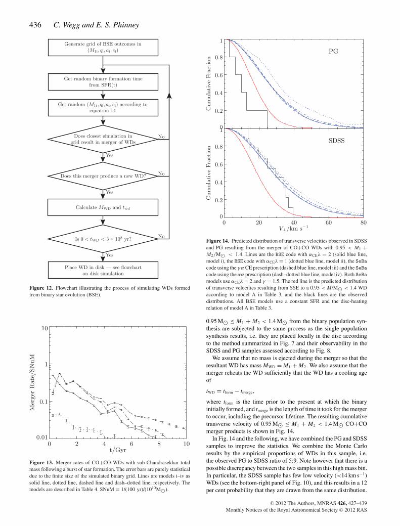
Figure 12. Flowchart illustrating the process of simulating WDs formedfrom binary star evolution (BSE).

Figure 13. Merger rates of CO+CO WDs with sub-Chandrasekhar totalmass following a burst of star formation. The error bars are purely statisticaldue to the finite size of the simulated binary grid. Lines are models i–iv assolid line, dotted line, dashed line and dash–dotted line, respectively. Themodels are described in Table 4. SNuM ≡ 1/(100 yr)/(1010M�).

Figure 14. Predicted distribution of transverse velocities observed in SDSSand PG resulting from the merger of CO+CO WDs with 0.95 < M1 +M2/M� < 1.4. Lines are the BSE code with αCEλ = 2 (solid blue line,model i), the BSE code with αCEλ = 1 (dotted blue line, model ii), the SeBacode using the γα CE prescription (dashed blue line, model iii) and the SeBacode using the αα prescription (dash–dotted blue line, model iv). Both SeBamodels use αCEλ = 2 and γ = 1.5. The red line is the predicted distributionof transverse velocities resulting from SSE to a 0.95 < M/M� < 1.4 WDaccording to model A in Table 3, and the black lines are the observeddistributions. All BSE models use a constant SFR and the disc-heatingrelation of model A in Table 3.

0.95 M� ≤ M1 + M2 < 1.4 M� from the binary population syn-thesis are subjected to the same process as the single populationsynthesis results, i.e. they are placed locally in the disc accordingto the method summarized in Fig. 7 and their observability in theSDSS and PG samples assessed according to Fig. 8.

We assume that no mass is ejected during the merger so that theresultant WD has mass MWD = M1 + M2. We also assume that themerger reheats the WD sufficiently that the WD has a cooling ageof

tWD = tform − tmerge,

where tform is the time prior to the present at which the binaryinitially formed, and tmerge is the length of time it took for the mergerto occur, including the precursor lifetime. The resulting cumulativetransverse velocity of 0.95 M� ≤ M1 + M2 < 1.4 M� CO+COmerger products is shown in Fig. 14.

In Fig. 14 and the following, we have combined the PG and SDSSsamples to improve the statistics. We combine the Monte Carloresults by the empirical proportions of WDs in this sample, i.e.the observed PG to SDSS ratio of 5:9. Note however that there is apossible discrepancy between the two samples in this high mass bin.In particular, the SDSS sample has few low velocity (<14 km s−1)WDs (see the bottom-right panel of Fig. 10), and this results in a 12per cent probability that they are drawn from the same distribution.



The distribution of transverse velocities in Fig. 14 shows that de-spite the uncertainties in binary evolution resulting in very differentbinary histories (Fig. 11) and overall merger rates (Fig. 13), theresultant velocity distributions are very similar. This is a result ofthe ∼t−1 merger time distribution at late times discussed previously.

The results in Fig. 14 naturally lead to the question of what frac-tion of mergers is consistent with the data to be addressed. We wishto assess the fraction of high-mass galactic WDs formed by binarymergers (BSE) which we parametrize by θ . This results in a frac-tion 1 − θ from SSE. To assess a value of θ for a given SSE andBSE Monte Carlo realization, we first calculate the galactic forma-tion rate of high-mass WDs from SSE and BSE in this realization,which we denote SSE and BSE, respectively. Then, for both PGand SDSS we make α copies of the BSE objects simulated as ob-served, and β copies of objects simulated as observed from SSE.Assuming that equal numbers of objects were simulated in both theBSE and SSE realizations, the two simulated samples combinedhave a galactic BSE fraction of

θ = β BSE

β BSE + α SSE.

To test whether the data are consistent with this realization, weuse the two-sample Anderson–Darling statistic (Pettitt 1976). TheAnderson–Darling test considers the difference between the sam-ples across the entire distribution, and so is more statistically power-ful than the more commonly used Kolmogorov–Smirnov test whichdepends only on the extremum. The number of simulated WDs isalways much larger, by at least a factor of 10, than the numberobserved.

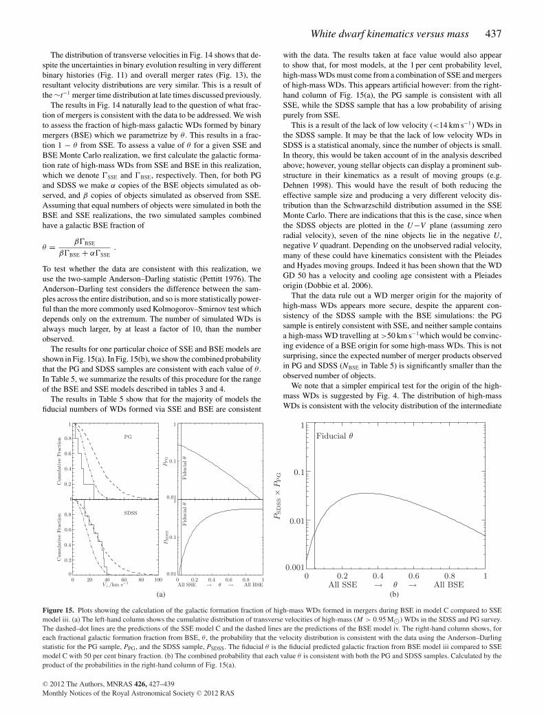
The results for one particular choice of SSE and BSE models areshown in Fig. 15(a). In Fig. 15(b), we show the combined probabilitythat the PG and SDSS samples are consistent with each value of θ .In Table 5, we summarize the results of this procedure for the rangeof the BSE and SSE models described in tables 3 and 4.

The results in Table 5 show that for the majority of models thefiducial numbers of WDs formed via SSE and BSE are consistent

with the data. The results taken at face value would also appearto show that, for most models, at the 1 per cent probability level,high-mass WDs must come from a combination of SSE and mergersof high-mass WDs. This appears artificial however: from the right-hand column of Fig. 15(a), the PG sample is consistent with allSSE, while the SDSS sample that has a low probability of arisingpurely from SSE.

This is a result of the lack of low velocity (<14 km s−1) WDs inthe SDSS sample. It may be that the lack of low velocity WDs inSDSS is a statistical anomaly, since the number of objects is small.In theory, this would be taken account of in the analysis describedabove; however, young stellar objects can display a prominent sub-structure in their kinematics as a result of moving groups (e.g.Dehnen 1998). This would have the result of both reducing theeffective sample size and producing a very different velocity dis-tribution than the Schwarzschild distribution assumed in the SSEMonte Carlo. There are indications that this is the case, since whenthe SDSS objects are plotted in the U−V plane (assuming zeroradial velocity), seven of the nine objects lie in the negative U,negative V quadrant. Depending on the unobserved radial velocity,many of these could have kinematics consistent with the Pleiadesand Hyades moving groups. Indeed it has been shown that the WDGD 50 has a velocity and cooling age consistent with a Pleiadesorigin (Dobbie et al. 2006).

That the data rule out a WD merger origin for the majority ofhigh-mass WDs appears more secure, despite the apparent con-sistency of the SDSS sample with the BSE simulations: the PGsample is entirely consistent with SSE, and neither sample containsa high-mass WD travelling at >50 km s−1which would be convinc-ing evidence of a BSE origin for some high-mass WDs. This is notsurprising, since the expected number of merger products observedin PG and SDSS (NBSE in Table 5) is significantly smaller than theobserved number of objects.

We note that a simpler empirical test for the origin of the high-mass WDs is suggested by Fig. 4. The distribution of high-massWDs is consistent with the velocity distribution of the intermediate

Figure 15. Plots showing the calculation of the galactic formation fraction of high-mass WDs formed in mergers during BSE in model C compared to SSEmodel iii. (a) The left-hand column shows the cumulative distribution of transverse velocities of high-mass (M > 0.95 M�) WDs in the SDSS and PG survey.The dashed–dot lines are the predictions of the SSE model C and the dashed lines are the predictions of the BSE model iv. The right-hand column shows, foreach fractional galactic formation fraction from BSE, θ , the probability that the velocity distribution is consistent with the data using the Anderson–Darlingstatistic for the PG sample, PPG, and the SDSS sample, PSDSS. The fiducial θ is the fiducial predicted galactic fraction from BSE model iii compared to SSEmodel C with 50 per cent binary fraction. (b) The combined probability that each value θ is consistent with both the PG and SDSS samples. Calculated by theproduct of the probabilities in the right-hand column of Fig. 15(a).



Table 5. Summary of the results of calculation of the fraction of high-mass WDs formed in mergers compared to SSE. The SSE models are describedin Table 3 and the BSE models are described in Table 4. BSE is the galactic formation rate (in yr−1) from BSE assuming that the merger of twoCO WDs with combined mass between 0.95 and 1.4 M� results in a high-mass WD. SSE is the galactic formation rate from SSE. θ is the galacticfraction of high-mass WDs formed from BSE so that the fiducial value is given by θfid ≡ SSE

BSE+ SSE. The numbers NSSE and NBSE are the predicted

observed numbers from SSE and BSE evolution, respectively, in the PG and SDSS samples. P(θfid) is the probability that both the PG and SDSSvelocity distributions are consistent with θfid using the Anderson–Darling statistic. θ (P > 0.05) is the range of θ values which have a probability ofbeing consistent with the data greater than 1 per cent. The fiducial value of θ is calculated assuming a 50 per cent binary fraction (i.e. two-thirds of allstars formed in binaries). Both SSE and BSE models use the same disc-heating model and star formation history: model C of Table 3 for the constantSFR models, and model D for the exponential.

SFR SSE model BSE model BSE SSE θfid PG SDSS P(θfid) θ (P > 0.01)NSSE NBSE NSSE NBSE

Const C i 0.0006 0.03 0.02 7 0.1 17 0.9 0.02 0.09–0.9C ii 0.0001 0.03 0.005 7 0.02 17 0.1 0.005 0.08–0.8C iii 0.001 0.03 0.04 7 0.3 17 2.0 0.04 0.08–0.8C iv 0.001 0.03 0.04 7 0.3 17 2.0 0.04 0.09–1.0

Exp D i 0.0007 0.02 0.04 6 0.1 13 1.0 0.04 0.1–0.9D ii 0.0002 0.02 0.01 6 0.02 13 0.2 0.01 0.2–0.8D iii 0.001 0.02 0.07 6 0.3 13 3.0 0.07 0.1–0.9D iv 0.001 0.02 0.06 6 0.3 13 2.0 0.06 0.2–0.9

group that displays the kinematics of young objects at the 13 percent level by the Anderson–Darling test. This ignores the selectioneffects which the Monte Carlo simulation addresses, but does sug-gest that the entire combined group of high-mass WDs is broadlyconsistent with SSE.

6 SC A L E H E I G H T S

One of the key results of this study is that hot WDs of mass�0.75 M� had much shorter main sequence lifetimes than theirlower mass counterparts, and hence their kinematics are character-istic of young stars. A direct result of this is that these higher massWDs will have reduced scale height. This is vitally important toconsider when calculating the formation rate as a function of massusing local samples such as in Liebert et al. (2005) or Kepler et al.(2007) or producing galactic WD simulations such as Nelemanset al. (2001).

Unfortunately, neither the SDSS nor the PG sample allows accu-rate direct determination of the scale height of each WD population,particularly the rare and less luminous high-mass groups. Instead,here we list the expected scale height by comparison with the SSEmodels that appear to accurately describe the kinematics. We dothis to allow simple initial corrections without resorting to the sim-ulations of the type performed in this work. The scale height, h, wasdefined through

ν(z) = ν0 sech2( z

2h

), (12)

where ν(z) is the stellar number density in terms of the height abovethe plane of the galactic disc, z. The scale height, h, was estimated byconstraining equation (12) to give both the correct overall numberand central WD density, ν0. We choose this method since the mostcommon usage of the scale height is to calculate galactic birthratesfrom local densities. The results are give in Table 6. Note that thehigher mass groups smaller scale height results in a local densityenhanced by more than a factor of 2 over the more common low-mass group. In particular, the apparent excess of high-mass WDsfound in the PG survey (discussed in section 6 of Liebert et al. 2005)can be naturally explained by their lower scale height, which causesa high abundance in this relatively local survey. That the number ofhigh-mass WDs is consistent with single star expectations in PG isconfirmed by the number of expected WDs from SSE in Table 5.

Table 6. Scale heights, h, defined through equa-tion (12) for three different mass groups. h is cal-culated by matching the central density and overallnumber to the simulations described in Section 4.2.

Mlow (M�) Mhigh (M�) h (pc)

0.45 0.75 1200.75 0.95 580.95 1.40 54

7 SU M M A RY

We have analysed the kinematics of young (<3 × 108 yr) DA WDsfrom both the PG survey and the SDSS and find a strong connectionbetween their mass and kinematics: low-mass WDs (0.45 M� ≤M1 + M2 < 0.75 M�) display the kinematics of old stars, withhigher velocity dispersion (∼46 km s−1) and asymmetric drift, whilehigher mass WDs (0.75 M� ≤ M1 + M2 < 0.95 M�) displaythe kinematics of young stars with a velocity dispersion of only∼19 km s−1. We have shown in Section 4 that this is expected due tothe shorter precursor lifetime of the more massive progenitors, andthat there is agreement both on simple analytic grounds (Section 4.1)and more quantitative Monte Carlo simulations of the PG and SDSSsamples (Section 4.2).

A further key conclusion is that the WD scale height and itsvariation with age and mass are vitally important to consider whencalculating birth rates based on local samples (Section 6).

In addition, we have separately analysed the highest mass WDs(M > 0.95 M�, Section 5), since it has been suggested that manyof these formed as a result of the merger of two lower mass COWDs. We find at present a discrepancy in the SDSS velocity dis-tribution where no high-mass WDs with transverse velocity lessthan 14 km s−1is detected. This results in a velocity distribution thatwithin our statistical framework is inconsistent with purely SSE.We argue that this is likely to an anomaly, either be a statistical or aresult of a number of these WDs being members of moving groups.We find that, even under the most optimistic binary evolution mod-els, we would only expect to find three WDs formed via WD binarymergers and that the apparent excess of high-mass WDs found inPG is caused by their reduced scale height. In addition, we notethe kinematic ‘smoking gun’ of some fraction of high-mass WDs



coming from binary evolution would be high-mass WDs travellingat >50 km s−1, of which none are found in PG or SDSS.

AC K N OW L E D G M E N T S

CW gratefully acknowledges many useful discussions with NateBode. Support for this work was provided by NASA BEFS grantNNX-07AH06G.

R E F E R E N C E S

Anselowitz T., Wasatonic R., Matthews K., Sion E. M., McCook G. P., 1999,PASP, 111, 702

Bergeron P. et al., 2011, ApJ, 737, 28Catalan S., Isern J., Garcıa-Berro E., Ribas I., 2008, MNRAS, 387, 1693Dehnen W., 1998, AJ, 115, 2384Dehnen W., Binney J., 1998, MNRAS, 298, 387Dobbie P., Napiwotzki R., Lodieu N., Burleigh M., Barstow M., Jameson

R., 2006, MNRAS, 373, L45Eisenstein D. J. et al., 2006, ApJS, 167, 40Feast M., Whitelock P., 1997, MNRAS, 291, 683Fontaine G., Brassard P., Bergeron P., 2001, PASP, 113, 409Girardi L., Bressan A., Bertelli G., Chiosi C., 2000, A&AS, 141, 371Guseinov O. K., Novruzova K. I., Rustamov I. S., 1983, Ap&SS, 97, 305Han Z., 1998, MNRAS, 296, 1019Holberg J. B., Bergeron P., 2006, AJ, 132, 1221Holmberg J., Flynn C., 2000, MNRAS, 313, 209Hurley J. R., Pols O. R., Tout C. A., 2000, MNRAS, 315, 543Just A., Jahreiß H., 2010, MNRAS, 402, 461Kepler S. O., Kleinman S. J., Nitta A., Koester D., Castanheira B. G.,

Giovannini O., Costa A. F. M., Althaus L. G., 2007, MNRAS, 375, 1315Kleinman S. J. et al., 2004, ApJ, 607, 426Kowalski P. M., Saumon D., 2006, ApJ, 651, L137Kroupa P., 2001, MNRAS, 322, 231Liebert J., Bergeron P., Holberg J. B., 2005, ApJS, 156, 47Maoz D., Sharon K., Gal-Yam A., 2010, ApJ, 722, 1879Miller G. E., Scalo J. M., 1979, ApJS, 41, 513Munn J. A. et al., 2004, AJ, 127, 3034Munn J. A. et al., 2008, AJ, 136, 895Nelemans G., Yungelson L. R., Zwart S. F. P., Verbunt F., 2001, A&A, 365,

491Nordstrom B. et al., 2004, A&A, 418, 989Oppenheimer B. R., Hambly N. C., Digby A. P., Hodgkin S. T., Saumon D.,

2001, Sci, 292, 698Pauli E.-M., Napiwotzki R., Heber U., Altmann M., Odenkirchen M., 2006,

A&A, 447, 173Pettitt A., 1976, Biometrika, 63, 161Ratnatunga K. U., Bahcall J. N., Casertano S., 1989, ApJ, 339, 106Reid I. N., 2005, ARA&A, 43, 247Roeser S., Demleitner M., Schilbach E., 2010, AJ, 139, 2440Schlegel D. J., Finkbeiner D. P., Davis M., 1998, ApJ, 500, 525Seabroke G. M., Gilmore G., 2007, MNRAS, 380, 1348Serenelli A. M., Althaus L. G., Rohrmann R. D., Benvenuto O. G., 2001,

MNRAS, 325, 607Sion E. M., Fritz M. L., McMullin J. P., Lallo M. D., 1988, AJ, 96, 251Tremblay P.-E., Bergeron P., Gianninas A., 2011, ApJ, 730, 128Vennes S., 1999, ApJ, 525, 995Wielen R., 1977, A&A, 60, 263Wood M. A., 1995, in Koester D., Werner K., eds, Lecture Notes in Physics

Vol. 443, White Dwarfs. Springer Verlag, Berlin, p. 41

A P P E N D I X A : LI K E L I H O O D S

Here we give our expressions for the proper motion likelihoods ofan individual object. These largely follow Ratnatunga, Bahcall &

Casertano (1989), modified to include errors in proper motion. Weignore errors in the sky position (�, b), which are small.

Assuming a Schwarzschild distribution function, then, in coordi-nates aligned with the principle axes of the velocity ellipsoid,

f (V ) = 1√8π3σ1σ2σ3

exp(−(V − V0)T · � · (V − V0)

), (A1)

where � = diag(1/2σ1, 1/2σ2, 1/2σ3) and V0 is the mean velocity.Ignoring errors in distance, we then rotate to axes aligned with thesky plane, and integrate over the unobserved radial velocity, which,in this case, is a nuisance parameter.

We define, �, to be the dispersion tensor rotated into the coordi-nate system, (�, b, d), aligned with the sky plane. This will be givenby � = R · �, where R is a rotation matrix (given explicitly asequation A4 in Ratnatunga et al. 1989). The probability distribution,after integrating over the radial velocity as a nuisance parameter, isan ellipsoid in the sky plane

p(vl, vb) = C ′ exp[−α(v� − v�)2 − β(vb − vb)2

−2γ (v� − v�)(vb − vb)], (A2)

where v� and v� are the components of V0 in the directions of l andb (which can be obtained via (v�, vb, vd ) = R · V0) and α, β, γ andC′ are given by

α = �22 − �212/�11, (A3)

β = �33 − �213/�11, (A4)

γ = �23 − �12�13/�11, (A5)

C ′ =√

αβ − γ 2/π. (A6)

For each object, we have measurements of vl and vb, togetherwith an associated velocity error σ . Integrating over the ‘true’ vl

and vb gives the log likelihood used in equation (9) as

logLi(vobs� , vobs

b ) ≡ log∫

dVf (V )P(

V |vobs� , vobs

b , σ)

= log C ′′ − δ

(α + δ)(β + δ) − γ 2

×[(�v2

b + �v2� )(αβ − γ 2)

+ δ(β�v2

b + α�v2� + 2γ�v��vb

)], (A7)

where

δ = 1/2σ 2, (A8)

�v� = vobs� − v�, (A9)

�vb = vobsb − vb, (A10)

C ′′ = C ′ δ√π√

(α + δ)(β + δ) − γ 2(A11)

= δ

√αβ − γ 2

π3[(α + δ)(β + δ) − γ 2]. (A12)

Note that for small error, δ → ∞, and equation (A7) reduces to thelog of equation (A2) as expected.

This paper has been typeset from a TEX/LATEX file prepared by the author.


white dwarf kinematics versus mass - core · white dwarf kinematics versus mass 429 to the distance...

Documents