HAL Id: hal-00805116https://hal.archives-ouvertes.fr/hal-00805116v3

Preprint submitted on 5 Aug 2016

HAL is a multi-disciplinary open accessarchive for the deposit and dissemination of sci-entific research documents, whether they are pub-lished or not. The documents may come fromteaching and research institutions in France orabroad, or from public or private research centers.

L’archive ouverte pluridisciplinaire HAL, estdestinée au dépôt et à la diffusion de documentsscientifiques de niveau recherche, publiés ou non,émanant des établissements d’enseignement et derecherche français ou étrangers, des laboratoirespublics ou privés.

Where in cities do ”rich” and ”poor” people live? Theurban economics model revisited

Rémi Lemoy, Charles Raux, Pablo Jensen

To cite this version:Rémi Lemoy, Charles Raux, Pablo Jensen. Where in cities do ”rich” and ”poor” people live? Theurban economics model revisited. 2013. �hal-00805116v3�

Where in cities do “rich” and “poor” people live? The urban economics modelrevisited

Rémi Lemoya,b, Charles Rauxb, Pablo Jensenc,d

aUniversity of Luxembourg, Maison des Sciences Humaines, 11 Porte des Sciences, L-4366 Esch-Belval, LuxembourgbLAET (Transport, Urban Planning and Economics Laboratory), CNRS and University of Lyon, Lyon, France

cLaboratoire de Physique, Ecole Normale Supérieure de Lyon, CNRS and University of Lyon, Lyon, FrancedIXXI (Institut Rhônalpin des Systèmes Complexes), Lyon, France

Abstract

In this work, we exploit the power of the Alonso-Mills-Muth (AMM) urban economics model andshow that various utility functions and plausible conditions offer alternative explanations of house-holds’ location by income within a city. These include the existence of a “rich” center and morecomplex socio-spatial urban forms, for instance alternating a rich center, poor suburbs and a richouter ring, which have not yet been derived from the AMM model to our knowledge. In doing so wecombine analytical ideas and illustrations by the means of an agent-based model. The hypothesisof a central or non-central amenity is also studied, leading to different insights on the issue.

Introduction

In a widely cited paper, Jan K. Brueckner, Jacques-François Thisse and Yves Zenou (1999)asked “Why is central Paris rich and downtown Detroit poor?” They pointed at the “locationalindeterminacy” of the Alonso-Mills-Muth (AMM) monocentric model which identifies two opposingforces: on the one hand the preference of the high income households for housing consumption drivesthem to the outskirts, on the other hand their high opportunity cost of commuting time drives themtoward the job center. Depending on local conditions regarding the evolution of commuting cost andhousing consumption with respect to income, rich households may tend to live either in the centeror in the suburbs. In order to overcome this indeterminacy Brueckner, Thisse and Zenou propose anamenity-based theory which links the location of income groups to the spatial pattern of (central)amenities and hence to city idiosyncracies.

The aim of this paper is to enrich the approach of Brueckner, Thisse and Zenou, based on theAMM urban economics model. We show that various utility functions can be used in this frameworkto obtain a “rich” center, and also more complex socio-spatial urban forms. A special feature of thiswork is the use of agent-based simulations besides analytical ideas.

Indeed, agent-based models and more generally numerical simulations are interesting tools givingcomplementary results when related to analytical resolution. We build here on a previous work,Lemoy et al. (2013), which presents an agent-based model reproducing accurately the results of thestandard urban economics model (AMM model). We use this agent-based simulation frameworkwith a population of agents separated in two income groups, in order to study the question of the

Email addresses: remilemoy@gmail.com (Rémi Lemoy), charles.raux@let.ish-lyon.cnrs.fr (Charles Raux),pablo.jensen@ens-lyon.fr (Pablo Jensen)

August 5, 2016

socio-spatial structure of cities. We keep the two “sketch” cities as in Brueckner et al. (1999), that isto say the "European" type city (like Paris for instance), with schematically speaking, a rich centerand a poor periphery, and the "North American" city (like Detroit), with a poorer center and richerhouseholds in the periphery. This last configuration is the usual result of the AMM model whenseveral income groups are introduced.

Lemoy et al. (2010) present a discussion on the difficulty to represent in a satisfactory way the"European" type city with the standard AMM model. An important reason for this difficulty isthe fact that they consider a log-linear (or Cobb-Douglas) utility function, as most studies usingconcrete examples of utility functions. This function is very convenient for analytical resolution andhas some interesting properties for calibration, if one supposes that the budget shares of compositegood and housing do not vary with income.

However, this hypothesis can be challenged since the share of income spent on housing is shownempirically to vary with income. In a first stage a Cobb Douglas function is still used, but takinginto account various shares of housing expenses for the two income groups. An analytical insightand an illustration with our agent-based model show that, depending on the relative values of thecity radius and a critical radius depending on model parameters, a more substantial pattern mayemerge, for instance a rich center (“European”-type city) surrounded by a poor suburb and then arich periphery.

This last urban form reflects a U-shaped curve of the income as a function of the distance tothe city center. This result can be linked to empirical evidence in several big French cities. Forinstance in Paris metropolitan area the richest districts are observed in the city center, extendingup to the western suburbs and outskirts, while other (and especially northern) suburbs gather lowerincome districts, followed by outskirts gathering again average and upper income districts (Françoiset al. (2011)). Other urban areas like Lyon, Toulouse and Bordeaux show also a concentration of richhouseholds in the city center and similar alternations of lower and upper income districts when goingaway from the center (Caubel (2005)). In addition, the U-shaped curve can also be seen in olderNorth American cities, like New York, Chicago or Philadelphia (see Glaeser et al. (2008)), which arecloser to the "European" pattern than to the usual socio-spatial structure of North American cities.

Since the Cobb-Douglas utility function fixes budget shares, there is no possible substitutionbetween variables. In order to overcome this limitation, we use in a second stage a constant elasticityof substitution utility function (CES, see Chung (1994)), with an exogenous amenity, as in Brueckneret al. (1999). The agent-based model is then able to reproduce a "European" urban social structure.However, here again it is shown that depending on the distance to the center, bid-rent curves of richand poor households may intersect again, yielding a rich periphery and hence the U-shaped incomevariation according to the distance from the center. Moreover, thanks to the agent-based model,we illustrate the effect of a displacement of the amenity away from the center and show that morecomplex socio-spatial structures can be found.

The remainder of the paper is structured as follows. In the first section the agent-based modelis briefly presented along with the mechanisms introduced to reach an equilibrium corresponding tothe analytical one. Section 2 and section 3 present respectively the analyses with the Cobb-Douglasutility function and the CES utility function. Discussion and conclusion are given in the final section.

1. An agent-based model of urban economics

We first present rapidly the numerical simulations used in Lemoy et al. (2013) and in the presentwork to find the equilibrium of the AMM model in cases where analytical resolution is difficult.

2

The use of these simulations to solve for the equilibrium of the AMM model can be linked to theMonte Carlo method (Binder and Heermann (2010)) or to local search optimization algorithms incomputer science (Lenstra (2003)). We use an agent-based framework, where a population of Nagents is given behavior rules which reproduce the competition for land in the AMM model.

Agents live on a 2-dimensional grid representing the urban space, which is polarized by thepresence of a central business district (CBD). All agents work in the CBD and commute daily forwork, with an associated transport cost which is proportional to the distance traveled. This distance,which we denote by x, corresponds to the distance between the housing location of an agent andthe CBD, and the associated transport cost is then tx, with t the transport cost per unit distance.

Agents are divided in two groups of incomes Yr and Yp for rich and poor, with Yr > Yp. Theirincome is spent entirely between transport expenses for daily commuting tx, housing expenses, andthe consumption of a composite good z of unit price, representing all other consumptions which donot depend on x. Housing expenses are written ps, with p the price of a unit surface of housing atthe considered location, and s the surface of the housing lot. Price p is a variable attached to eachcell of the simulation grid. Cells have a fixed surface stot, and the side of a cell is supposed to be ofunit length. However cells may welcome several housing lots, that is to say density is endogenous.

Agents wish to maximize their economic welfare, represented by a utility function U(z, s) de-pending on consumptions of composite good z and housing s. The budget constraint can be writtenYi = zi+ tix+psi, with i = r, p (for rich and poor agents respectively). At given price p and locationx, agents have optimal composite good and housing consumptions. With a Cobb-Douglas utilityfunction Ui = zαi s

βi with α and β positive parameters such that α+β = 1, this yields zi = α(Yi−tix)

and psi = β(Yi − tix) for i = r, p (see Chung (1994)).The dynamics of this agent-based model consists in a simple move and bidding mechanism.

Simulations start with a random configuration: agents are located at random on the simulationspace. The prices in all cells are initialized at an agricultural rent Ra, which is a minimal price inthe system, corresponding to an agricultural use of land. At each time step of the model, an agentand a cell are chosen at random. The agent, having initially utility U0, moves into the cell if thisone provides him with a higher utility U1 at its current price pn, and enough space. However, theagent needs to propose a bid pn+1 on the price of the cell, which has the following form

pn+1 = pn(1 + εU1 − U0

U0)

where ε is a positive parameter controlling the magnitude of this bid.This bidding mechanism describes how price increases in attractive cells. It competes with the

decreasing price of cells which are fully or partially vacant. Indeed, vacancy indicates that thesecells are not attractive at their current price pn, which the landowner decreases to pn+1 following

pn+1 = pn − (pn −Ra × 0.9)/Tp

where Tp is a parameter controlling the speed of this decrease of prices. This formula yields anexponential decrease of the price, which goes to the minimal price corresponding to the agriculturalrent Ra after a finite number of steps. If the price reaches Ra, this decrease stops.

As Lemoy et al. (2013) show, this agent-based system reaches a discrete version of the analyticalequilibrium of the AMM model. Parameters ε and Tp can have a dependency on the occupation rateof cells in order to accelerate the convergence to the equilibrium. Throughout this paper, we willuse the values ε = 0.5 and Tp = 100. These behavior rules provide a robust mechanism pushing the

3

agent-based system towards the equilibrium of the AMM model. Indeed, this equilibrium can alsobe reached in cases where analytical treatment is difficult, as in the case of our present study of thesocio-spatial structure of cities.

2. A critical radius for income related location

As was shown in the previous section, the Cobb-Douglas utility function has the property to fixthe shares of income (net of transport cost) spent by the agent on different items. However, theempirical literature shows an evolution with income of the share of income spent by households onhousing. On average, when income increases, the share of income spent on housing decreases: seefor instance Accardo and Bugeja (2009) or Polacchini (1999) for evidence respectively in France andParis region; Cervero et al. (2006) for evidence in the USA.

Moreover, the value of time increases with income with an elasticity smaller than one (seefor instance Small (1992); Wardman (2001a,b)). In this section, we study the influence of thesefactors together – evolution with income of the value of time and of the share of income spenton housing – on the location choices of households within the AMM model. We still use a Cobb-Douglas utility function. However, we suppose here that the share of income spent on housingand composite good depends on income. With two income groups, this is taken into account byintroducing different parameters αr, βr and αp, βp in the utility functions of rich and poor agents.We still have αr+βr = αp+βp = 1, but rich agents spend a smaller part of their income on housing:βr < βp.

Following empirical literature the value of time is assumed to be higher for the rich income group.As a consequence, we postulate that the (unit distance) transport cost tr of rich agents is higherthan the transport cost tp of poor agents, tr > tp, due to the difference of time costs, supposing thatthe monetary part of the transport cost is the same for both income groups.

2.1. Critical distance and city boundaryThe condition which determines the social structure of the city is detailed in Fujita (1989) (or

Goffette-Nagot et al. (2000)): in the case of a continuum of income groups, the income group locatednear the center is the high income group if the income elasticity of marginal transport cost (pullingforce) is higher than the income elasticity of the demand for housing (pushing force). If the incomeelasticity of the demand for housing is higher, then the low income group is located near the center.

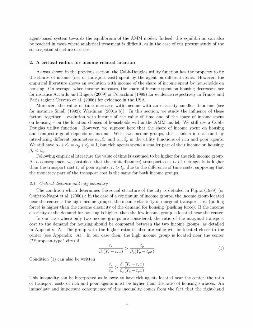
In our case where only two income groups are considered, the ratio of the marginal transportcost to the demand for housing should be compared between the two income groups, as detailedin Appendix A. The group with the higher ratio in absolute value will be located closer to thecenter (see Appendix A). In our case then, the high income group is located near the center("European-type" city) if

trβr(Yr − trx)

>tp

βp(Yp − tpx)(1)

Condition (1) can also be writtentrtp>βr(Yr − trx)

βp(Yp − tpx)

This inequality can be interpreted as follows: to have rich agents located near the center, the ratioof transport costs of rich and poor agents must be higher than the ratio of housing surfaces. Animmediate and important consequence of this inequality comes from the fact that the right-hand

4

side depends on the distance x to the center, whereas the left-hand side is constant, as we use alinear transport cost, proportional to the distance to the CBD. This condition yields richer urbanforms in the model than just rich households in the center and poorer ones in the periphery, or viceversa.

Indeed, a critical distance xc from the center can be defined, at which arc elasticities ε(t, Y ) andε(s, Y ) are equal. Beyond this distance of the center, the direction of the inequality (1) changes. Asa consequence, condition (1) can also be written

x < xc =βpYptr − βrYrtptrtp(βp − βr)

Then different social patterns can be observed in this model, depending on the value of xc and onthe radius of the city xb, the latter being fixed by the boundary conditions of the model, see Fujita(1989) for instance.

If xc ≤ 0, the model gives the standard result of the AMM model with two income groups: pooragents are located in the center of the city and rich agents in the periphery. This is usually seenas a representation of a "North American" city. On the contrary, if xc ≥ xb, the social pattern isreversed. Rich households are located in the center, and poorer ones in the periphery. This can beseen as a "European"-type city.

A different result can be found if 0 < xc < xb1. Indeed in this case, rich households tend to locate

closer to the center than poor households when their commuting distance x is such that 0 ≤ x < xc,and further from the center than poor households when xc < x < xb. We leave to further study thecomplete analytical treatment of this case, which would for instance compare the bid rent curves ofrich and poor agents within this model and show that they can intersect two times. In the followingsection, we use agent-based simulations to illustrate the results of this model in this special casewhere the critical radius is within the city boundary 0 < xc < xb.

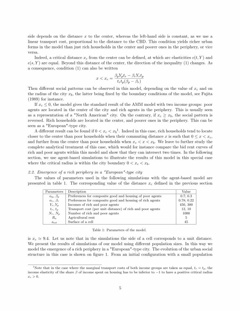
2.2. Emergence of a rich periphery in a "European"-type cityThe values of parameters used in the following simulations with the agent-based model are

presented in table 1. The corresponding value of the distance xc defined in the previous section

Parameters Description Valueαp, βp Preferences for composite good and housing of poor agents 0.7; 0.3αr, βr Preferences for composite good and housing of rich agents 0.78; 0.22Yr, Yp Incomes of rich and poor agents 450, 300tr, tp Transport cost (per unit distance) of rich and poor agents 12, 10Nr, Np Number of rich and poor agents 1000Ra Agricultural rent 5stot Surface of a cell 45

Table 1: Parameters of the model.

is xc ' 9.4. Let us note that in the simulations the side of a cell corresponds to a unit distance.We present the results of simulations of our model using different population sizes. In this way wemodel the emergence of a rich periphery in a "European"-type city. The evolution of the urban socialstructure in this case is shown on figure 1. From an initial configuration with a small population

1Note that in the case where the marginal transport costs of both income groups are taken as equal, tr = tp, theincome elasticity of the share β of income spent on housing has to be inferior to −1 to have a positive critical radiusxc > 0.

5

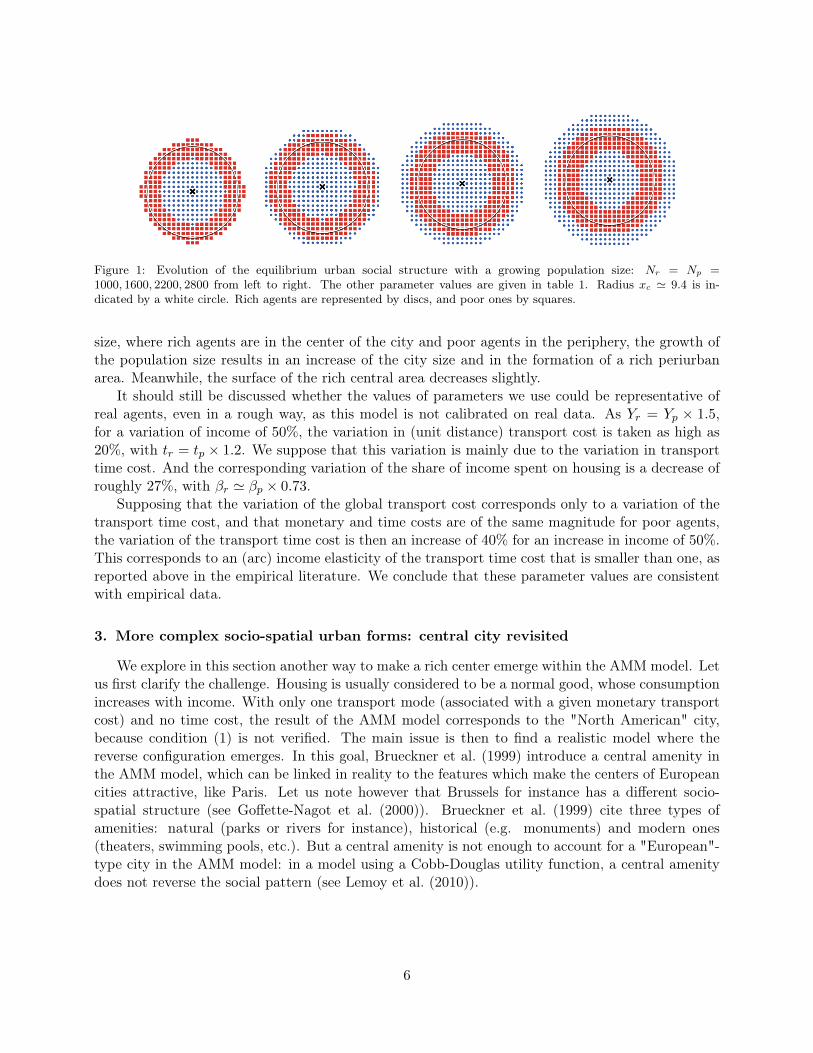
Figure 1: Evolution of the equilibrium urban social structure with a growing population size: Nr = Np =1000, 1600, 2200, 2800 from left to right. The other parameter values are given in table 1. Radius xc ' 9.4 is in-dicated by a white circle. Rich agents are represented by discs, and poor ones by squares.

size, where rich agents are in the center of the city and poor agents in the periphery, the growth ofthe population size results in an increase of the city size and in the formation of a rich periurbanarea. Meanwhile, the surface of the rich central area decreases slightly.

It should still be discussed whether the values of parameters we use could be representative ofreal agents, even in a rough way, as this model is not calibrated on real data. As Yr = Yp × 1.5,for a variation of income of 50%, the variation in (unit distance) transport cost is taken as high as20%, with tr = tp × 1.2. We suppose that this variation is mainly due to the variation in transporttime cost. And the corresponding variation of the share of income spent on housing is a decrease ofroughly 27%, with βr ' βp × 0.73.

Supposing that the variation of the global transport cost corresponds only to a variation of thetransport time cost, and that monetary and time costs are of the same magnitude for poor agents,the variation of the transport time cost is then an increase of 40% for an increase in income of 50%.This corresponds to an (arc) income elasticity of the transport time cost that is smaller than one, asreported above in the empirical literature. We conclude that these parameter values are consistentwith empirical data.

3. More complex socio-spatial urban forms: central city revisited

We explore in this section another way to make a rich center emerge within the AMM model. Letus first clarify the challenge. Housing is usually considered to be a normal good, whose consumptionincreases with income. With only one transport mode (associated with a given monetary transportcost) and no time cost, the result of the AMM model corresponds to the "North American" city,because condition (1) is not verified. The main issue is then to find a realistic model where thereverse configuration emerges. In this goal, Brueckner et al. (1999) introduce a central amenity inthe AMM model, which can be linked in reality to the features which make the centers of Europeancities attractive, like Paris. Let us note however that Brussels for instance has a different socio-spatial structure (see Goffette-Nagot et al. (2000)). Brueckner et al. (1999) cite three types ofamenities: natural (parks or rivers for instance), historical (e.g. monuments) and modern ones(theaters, swimming pools, etc.). But a central amenity is not enough to account for a "European"-type city in the AMM model: in a model using a Cobb-Douglas utility function, a central amenitydoes not reverse the social pattern (see Lemoy et al. (2010)).

6

3.1. Analytical discussionTo obtain this reversal, two conditions are given by Brueckner et al. (1999): the marginal val-

uation of amenities, after optimal choice of the housing consumption, must rise faster with incomethan housing consumption, and the gradient of the amenity function must be negative and large inabsolute value. An example of utility function satisfying the first condition is given by the constantelasticity of substitution (CES) utility function, which can be written:

UCES(z, s, a(y)) =(αz−ρ + βs−ρ + (1− α− β)a(y)−ρ

)−1/ρwhere the same notations are used as previously for z and s, α and β are now such that α+ β ≤ 1,and ρ is a real parameter. a(y) is a function describing the amenity, depending on the distance y tothe amenity center. The budget constraint is the same as in the previous section, with tr = tp = t:Yi = zi + tx + psi with i = r, p. σ = 1/(1 + ρ) is a parameter which is linked to the elasticityof substitution between variables (see Chung (1994)). Brueckner et al. (1999) show that the firstcondition (the marginal valuation of amenities rising faster with income than housing consumption)is valid if σ < 1. We use this CES utility function here, with ρ = 0.3 (σ ' 0.77), so that thiscondition is verified.

3.2. Variations on (non-)central amenity, rich center and rich peripheryThe amenity function a(y), depending on the distance y to the amenity center, must also be

chosen. We take the same function as Lemoy et al. (2010): a decreasing exponential a(y) = 1 +a0 exp(−y/b), with a0 determining the magnitude of the amenity at its origin and b the characteristicdistance of the amenity decrease. The optimal consumption of land (or housing) conditional on pricep and location x is

si =Yi − tx

(αp/β)σ + p

for i = r, p (see Chung (1994)). This expression is used in the agent-based model presented in section1, replacing the corresponding expression for the Cobb-Douglas function.

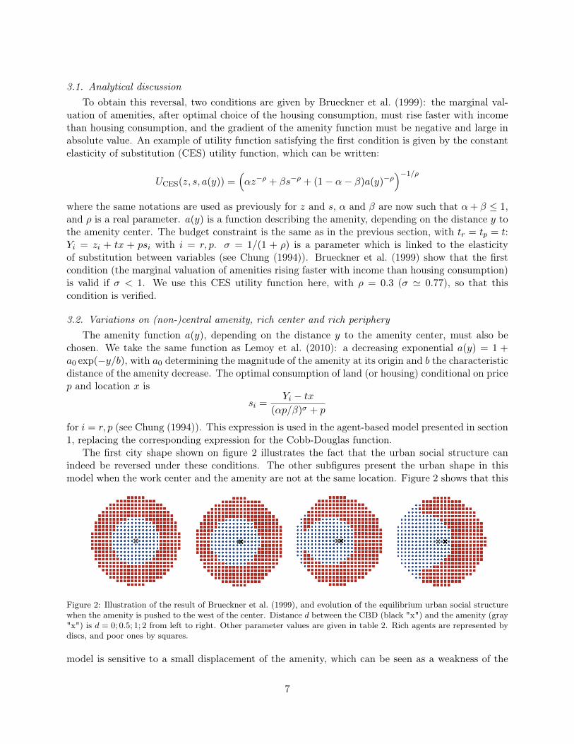
The first city shape shown on figure 2 illustrates the fact that the urban social structure canindeed be reversed under these conditions. The other subfigures present the urban shape in thismodel when the work center and the amenity are not at the same location. Figure 2 shows that this

Figure 2: Illustration of the result of Brueckner et al. (1999), and evolution of the equilibrium urban social structurewhen the amenity is pushed to the west of the center. Distance d between the CBD (black "x") and the amenity (gray"x") is d = 0; 0.5; 1; 2 from left to right. Other parameter values are given in table 2. Rich agents are represented bydiscs, and poor ones by squares.

model is sensitive to a small displacement of the amenity, which can be seen as a weakness of the

7

amenity center added here. Indeed in real cities, amenity and employment centers are probably notfound in the exact same locations. As the results show, even a small distance between both centershas an important impact on the urban socio-spatial structure in this model. The parameters usedare given in table 2.

Parameters Description Default valueα, β, ρ Parameters of the CES utility function 0.3Yr, Yp Incomes of rich and poor agents 450, 300t Transport cost (unit distance) 10

Nr, Np Number of rich and poor agents 2000Ra Agricultural rent 5stot Surface of a cell 100a0 Amenity function at the origin 5b Characteristic distance of decrease of the amenity 4

Table 2: Default parameters of the model reproducing the result of Brueckner et al. (1999)

Then we illustrate a fact which is not studied by Brueckner et al. (1999), but appears very easilyin our agent-based simulations. This result is in direct correspondence with the one presented inthe previous section: the condition which guarantees that the high income group is located near thecenter depends on the distance to the center. So that it may be verified close to the center and notfurther away. More precisely, we suppose with Brueckner et al. (1999) that there is a first radius x1at which the bid rent curves of rich and poor agents intersect. The condition mentioned before, thatthe gradient of the amenity function is negative and large in absolute value, is verified. So that richagents are located at x ≤ x1 and poorer ones at x ≥ x1.

But we suppose now that there is a second radius x2 > x1 at which these bid rent curves intersect.With the decreasing exponential form of the amenity function we have chosen, the amenity gradientdecreases in absolute value when x increases. This is why both curves can intersect again. So thatat this second intersection x2, the gradient of the amenity function can be small in absolute value,and rich agents are now driven to the periphery at x ≥ x2, while poor agents are located closer tothe center, at x ≤ x1.

Figure 3: Evolution of the equilibrium urban social structure when the amenity is pushed to the west of the center.The distance d between the CBD and the amenity is d = 0; 0.5; 1; 2 from left to right. The other parameter values aregiven by table 2, except a0 which has here a smaller value: a0 = 3. Same symbols as figure 2.

An urban structure similar to the last configuration presented in the previous section can beobserved in this case: a part of the high income group lives in the center, encompassed by a ringwhere the low income group is located. And further away lives the rest of the high income group,which benefits less of the amenity, but can afford bigger housing surfaces thanks to the lower landprices. This configuration is presented on figure 3, which uses the same parameter values as figure 2

8

(given by table 2), except that the intensity of the amenity function at its origin is smaller: a0 = 3.It can be noted that more complex amenity functions than the decreasing exponential form couldlead to social patterns which are even more complex than the patterns presented on figure 3.

Here also, we explore the results of the model when the amenity is not at the same location asthe CBD, and we find that the city’s social structure is very sensitive to this small displacementof the amenity. Paris is an empirical illustration of this case where various urban amenities likemonuments, museums and parks are located on the western half-side along with richer population(François et al. (2011)).

Discussion and conclusion

Two different frameworks are used with two income groups within the AMM model and yielda hybrid configuration corresponding to a "European" city structure with a rich suburb, which hasdifferent origins in each case.

In the first one, with a Cobb-Douglas utility function where the evolution with income of thebudget share of housing is taken into account, analytical calculations on income elasticities lead us todefine a critical distance at which the relative locational behaviors of income groups changes. Belowthis distance, the higher value of time of rich agents, combined with their lower budget share forhousing, leads them to choose small housing lots in the city center. Beyond this critical distance, theother part of the high income group is driven to the periphery by the desire to have bigger housinglots, allowed by smaller price in the periphery.

In the second framework, a study of the introduction of a central amenity in the AMM model,combined with a CES utility function, allows us to confirm the results of Brueckner et al. (1999), andto go further. A compromise between smaller housing lots and the benefit of a central amenity leadsa part of rich households to live in the city center, giving the same outcome as previously. However,beyond a specific distance the influence of the amenity is weak and the preference for housing takesover to drive another part of the rich households to the outskirts.

Indeed, like the first model, this second model can have as an outcome a "European"-type urbansocial structure, with rich agents in the center, poorer ones in the suburbs, and in addition an outerring of rich households. The first framework has the advantage, when compared with the second one,to avoid the exogenous introduction of an amenity, which is a bit frustrating from a modeling pointof view. In addition, because it does not have an exogenous amenity (which could still be addedin further work), its results are not sensitive to the location of the amenity, contrary to Brueckneret al. (1999)’s framework in two dimensions. On the other hand, this second framework can modelricher, non-isotropic urban structures.

Several perspectives of work can be drawn. The first and most important one concerns theissue of the calibration of urban models, to test more precisely their link with empirical data. Inparticular, the ideas studied here regarding European and North American city models should beinteresting to test on empirical data from both continents, if these can be gathered. This issue of thecalibration of urban models is a difficult one, which is probably not enough treated in the literature.

Another perspective is linked to the historical evolution of cities through population size andtransport cost (see for instance LeRoy and Sonstelie (1983)). Moreover, introducing two trans-port modes with various costs and speed in the model presented in section 2 is also an interestingperspective.

9

Acknowledgements

The authors thank gratefully Florence Goffette-Nagot (GATE, CNRS and University of Lyon)for her valuable comments at various stages of this research.

Appendix A. Socio-spatial structure and bid rent

In the case of a monocentric AMM model with two income groups2, let us derive here condition(1), which determines which income group is located closer to the center (see also Fujita (1989) orGoffette-Nagot et al. (2000)). The welfare of households is described by a utility function U(z, s)depending on their consumption of a composite good z and of housing surface s. These householdsalso have a budget constraint, which expresses the fact that their income Y is spent entirely betweentheir consumption of composite good z, their transport expenses T (x) and their housing expensesps: Y = z + T (x) + ps, where p is the rent per unit surface.

Due to their competition for land, agents are led to pay a rent corresponding to their bid rentΨ(x, u), which is the maximum rent (per unit surface) which they can pay at a distance x from thecenter, when their utility is at a level u. From the budget constraint, this bid rent can be expressedas

Ψ(x, u) = maxz,s

(Y − T (x)− z

s, s. t. U(z, s) = u

).

Let us now suppose that the expression of the utility function U(z, s) can be inverted in order toexpress the consumption of composite good Z(s, u) as a function of the consumption of housing sand of the utility level u. Then the bid rent can be rewritten as

Ψ(x, u) = maxs

(Y − T (x)− Z(s, u)

s

).

Using the enveloppe theorem, the gradient of the bid rent ∂Ψ/∂x can be computed:

∂Ψ

∂x= − T ′(x)

S(x, u),

where T ′ is the derivative of T and S(x, u) is the consumption of land which maximizes the bidrent at distance x and utility level u. As the transport cost T (x) is increasing with distance x, thisgradient is negative.

Let us consider now two income groups 1 and 2, with incomes Y1 and Y2, with two different bidrent curves Ψ1(x, u) and Ψ2(x, u). Then because of the competition for housing, these curves needto intersect somewhere in the city if both groups are to be located inside the city. Let us call x thedistance at which the curves intersect. As the gradients of bid rents are negative, the income groupwhich will be located closer to the center (at distances smaller than x) is the one whose bid rent hasthe largest gradient (in absolute value): income group 1 is located closer to the center if

T ′1(x)

S1(x, u)>

T ′2(x)

S2(x, u),

which leads to condition (1) with a Cobb-Douglas utility function (see Chung (1994)) and a lineartransport cost.

2This approach can be extended to more than two income groups.

10

References

Accardo, J., Bugeja, F., 2009. Le poids des dépenses de logement depuis vingt ans, in: Cinquanteans de consommation en France. Insee, Paris, pp. 33–47.

Binder, K., Heermann, D., 2010. Monte Carlo simulation in statistical physics: an introduction.Springer Science & Business Media.

Brueckner, J., Thisse, J., Zenou, Y., 1999. Why is central Paris rich and downtown Detroit poor?An amenity-based theory. European Economic Review 43, 91–107.

Caubel, D., 2005. Disparités territoriales infra-communales (IRIS-2000) selon les niveaux de vie etles positions sociales sur les aires urbaines de Lyon, Bordeaux, Paris, Toulouse, Dijon, Pau, Agenet Villefranche-sur-Saône. XLIème Colloque de l’ASRDLF "Villes et territoires face aux défis dela mondialisation". http://halshs.archives-ouvertes.fr/halshs-00095751.

Cervero, R., Chapple, K., Landis, J., Wachs, M., Duncan, M., Scholl, P.L., 2006. MAKING DO:HowWorking Families in Seven U.S. Metropolitan Areas Trade Off Housing Costs and CommutingTimes. Technical Report. UC Berkeley: Institute of Transportation Studies (UCB).

Chung, J.W., 1994. Utility and production functions: theory and applications. Blackwell Publishers.

François, J.C., Ribardière, A., Fleury, A., Mathian, H., Pavard, A., Saint-Julien, T., 2011. Lesdisparités de revenus des ménages franciliens - Analyse de l’évolution entre 1999 et 2007. Rapportpour la DREIA Ile-de-France. http://halshs.archives-ouvertes.fr/halshs-00737156.

Fujita, M., 1989. Urban Economic Theory. Cambridge University Press.

Glaeser, E.L., Kahn, M.E., Rappaport, J., 2008. Why do the poor live in cities? The role of publictransportation. Journal of Urban Economics 63, 1 – 24.

Goffette-Nagot, F., Thomas, I., Zenou, Y., 2000. Structure urbaine et revenu des ménages. Econom-ica, Paris. chapter 10. Economie Géographique : approches théoriques et empiriques.

Lemoy, R., Raux, C., Jensen, P., 2010. An agent-based model of residential patterns and social struc-ture in urban areas. Cybergeo: European Journal of Geography, Systems, Modelling, Geostatistics, article 512. http://cybergeo.revues.org/index23381.html.

Lemoy, R., Raux, C., Jensen, P., 2013. Exploring the polycentric city with multi-worker households:an agent-based microeconomic model. https://hal.archives-ouvertes.fr/hal-00602087.

Lenstra, J.K., 2003. Local search in combinatorial optimization. Princeton University Press.

LeRoy, S.F., Sonstelie, J., 1983. Paradise lost and regained: Transportation innovation, income, andresidential location. Journal of Urban Economics 13, 67–89.

Polacchini, A., 1999. Les dépenses des ménages franciliens pour le logement et les transports.Recherche Transports Sécurité 63.

Small, K.A., 1992. Urban transportation economics, in: Regional and Urban Economics II. HarwoodAcademic Publishers.

11

Wardman, M., 2001a. A review of British evidence on time and service quality valuations. Trans-portation Research Part E: Logistics and Transportation Review 37, 107 – 128.

Wardman, M., 2001b. Inter-temporal variations in the value of time. ITS Leeds Working Paper 566.

12