Research Institute of Industrial Economics

P.O. Box 55665

SE-102 15 Stockholm, Sweden

info@ifn.se

www.ifn.se

IFN Working Paper No. 900, 2012

When More Poor Means Less Poverty: On Income Inequality and Purchasing Power Andreas Bergh and Therese Nilsson

0

When more poor means less poverty: On

income inequality and purchasing power*

Andreas Bergh a,* Therese Nilsson b

Department of Economics, Box 7082, S-220 07 Lund, Sweden.

Research Institute of Industrial Economics, Box 55665, SE-102 15 Stockholm,

Sweden

Abstract

We show theoretically that the poor can benefit from price changes induced by

higher income inequality. As the number of poor in a society increases, or

when the income difference between rich and poor increases, the market for

products aimed towards the poor grows and such products become more

profitable. As a result, there are circumstances where an increase in poverty

associates with higher purchasing power of the poor. Using cross-country data

at two points in time on the price of rice and Big Mac hamburgers, we confirm

the relationship between inequality and purchasing power of the poor, and

show that it is robust to several control variables and also to a first-difference

specification.

JEL classification: D63; I3

Keywords: Inequality; Poverty; Prices; Purchasing power

a Research Institute of Industrial Economics and Department of Economics, Lund University, Sweden.

b Department of Economics, Lund University, and Research Institute of Industrial Economics (IFN), Sweden

E-mail addresses: Andreas.Bergh@nek.lu.se (A. Bergh) Therese.Nilsson@nek.lu.se (T. Nilsson)

* Corresponding author. Tel. +46 46 222 46 43. Fax +46 46 222 41 18.

* Financial support from the Jan Wallander and Tom Hedelius Research Foundation is gratefully acknowledged.

1

1. Introduction

In Africa, the retail chain Pick ‘N Pay is investing in the poorer parts of the

continent through low-price format stores, rather than expanding its existing

high and middle-end supermarkets. According to Weatherspoon and Reardon

(2003), this illustrates a trend: Supermarkets geared towards the poor.2

In China, rural farmers commonly used washing machines not only to wash

clothes, but also to wash vegetables. Haier, China’s biggest home appliance

manufacturer, responded by developing a washing machine with larger pipes

and providing instructions on how to clean vegetables in it. Anderson and

Billou (2007) use this particular example to illustrate that products are often

developed specially for the poor, rather than modeled on what has worked for

middle and high-income groups. Similarly, the Philippine telecom corporation

Smart Communications launched very small pricing packages on telecom that

matched the many poor consumer’s incomes and needs.

The examples above illustrate that, provided that the market is sufficiently big,

it is part of a profit maximizing strategy for firms to sell low priced products

and services to poor consumers. This paper notes that as a result, the price

structure will depend on the income distribution. As a somewhat counter-

intuitive result, higher income inequality will under some circumstances

associate with higher purchasing power and possibly improved welfare of the

poor.

As noted by Pendakur (2002), the price structure is usually ignored when

measuring economic inequality. The income of rich and poor in a country is

deflated using the same price vector.3 But if prices depend on the income

distribution, changes in the income distribution will not necessarily imply

similar changes in the distribution of purchasing power. The distributional

importance of the price structure is noted by Broda and Romalis (2009), who

show that much of the increase in income inequality in the US has been offset

by a relative decline in the prices of products that poorer consumers buy – the

so called Walmart-effect. We argue that this is no coincidence: Higher income

inequality will often imply higher demand for products targeted towards the

poor, and the increasing supply of these goods will mitigate adverse effects of

higher income inequality by its impact on the distribution of purchasing power.

2 Incidentally, the African supermarket chain Massmart was bought by Walmart in 2010, a chain that in the US has been highly successful providing low-price products to cash-constrained Americans. 3 Using Canadian data on regional price information and expenditure-dependent price deflators Pendakur (2002) shows that relative prices affect both the level of and year-to-year changes in family inequality.

2

This paper develops a simple model to analyze the effects of income inequality

on the distribution of purchasing power (section 2). The claim that higher

income inequality has purchasing power effects that are beneficial for the poor

is then tested empirically using data from middle- and high-income countries

on income inequality and the price of two inferior goods: rice and Big Mac

hamburgers (section 3). Section 4 concludes with some remarks on directions

for future research.

2. A simple model and some theoretical

considerations

Assume that society consists of two groups, rich and poor, with incomes λ>0

and ),,0( respectively. The poverty rate in the population is r.

Normalizing the population to 1, total income will be .1 rrY The

share of total income held by poor will be ./Yr From the properties of the

commonly used Gini-coefficient (see, for example, Lambert 1993), it follows

that coefficient will increase as the poverty rate increases from 0 to 0.5, and

then decrease as the poverty rate approaches 1. Assuming that r < 0.5, and

using G to denote the Gini-coefficient for income, our model has the

properties that a higher poverty rate increases the Gini-coefficient, and a higher

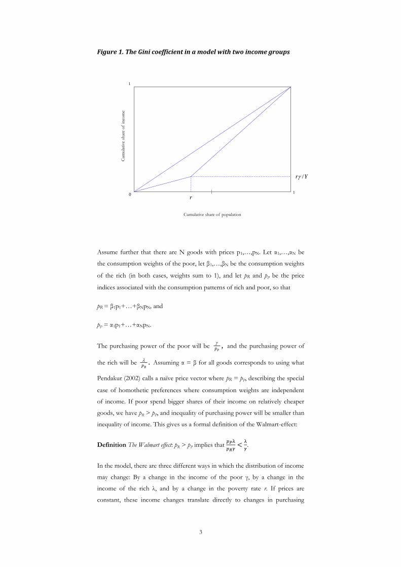
income of the poor decreases it: Gγ < 0 and Gr > 0. Figure 1 illustrates the

model graphically.

3

Figure 1. The Gini coefficient in a model with two income groups

Assume further that there are N goods with prices p1,…,pN. Let α1,…,αN be

the consumption weights of the poor, let β1,…,βN be the consumption weights

of the rich (in both cases, weights sum to 1), and let pR and pP be the price

indices associated with the consumption patterns of rich and poor, so that

pR = β1p1+…+βNpN, and

pP = α1p1+…+αNpN.

The purchasing power of the poor will be ,Pp

and the purchasing power of

the rich will be .Rp

Assuming α = β for all goods corresponds to using what

Pendakur (2002) calls a naïve price vector where pR = pP, describing the special

case of homothetic preferences where consumption weights are independent

of income. If poor spend bigger shares of their income on relatively cheaper

goods, we have pR > pP, and inequality of purchasing power will be smaller than

inequality of income. This gives us a formal definition of the Walmart-effect:

Definition The Walmart effect: pR > pP implies that

.

In the model, there are three different ways in which the distribution of income

may change: By a change in the income of the poor γ, by a change in the

income of the rich λ, and by a change in the poverty rate r. If prices are

constant, these income changes translate directly to changes in purchasing

Yr /

r 0

1

1

Cum

ula

tive

shar

eo

f in

com

e

Cumulative share of population

4

power. If prices depend on the income distribution, these changes will have

both direct and indirect effects on purchasing power.

Consider the change in purchasing power of the poor resulting from a change

in the income of the poor. The effect can be decomposed into a direct effect

caused by the change in income, and an indirect effect caused by changes in

the prices of goods consumed by the poor:

Pp

( )

( )

If prices are unaffected by a change in γ,

and the expression above

simplifies to

. Similarly, the change in purchasing power of the poor resulting

from a change in the income of the rich will be

Pp

( )

Finally, the change in purchasing power of the poor resulting from a change in

the poverty rate will be

Pp

( )

Clearly, the signs of the derivatives

,

, and

are important. In the

short run, changes in γ, λ and r will lead to demand shifts causing short run

price changes, but as the supply side adapts, prices will reflect the new income

structure of the economy.

Consistent with the anecdotal evidence cited in section 1,

follows

from the presence of fixed production costs: A higher poverty rate implies a

larger market for inferior products demanded by the poor. We refer to this as

the market size effect:

Definition The market size effect:

Empirical evidence (see e.g. Deaton and Muellbauer 1980) and the anecdotal

story on washing machines in section 1 suggest that consumer preferences are

non-homothetic. Clearly, firms may also meet fixed costs in supplying different

goods to rich and poor consumers, in which case the profitability of product

differentiation depends on the income difference between rich and poor, δ = λ

– γ, being sufficiently large. We refer to this as the market segregations effect:

5

Definition The market segregation effect:

As defined, pP decreases both when the poor become poorer and when the rich

become richer.

Intuitively, both purchasing power effects work through the mechanism that

inferior goods will be part of a profit maximizing strategy for firms only if the

demanded quantity is high enough. This will be true if the poor are sufficiently

numerous, (the market size effect), or if the income distance between rich and

poor is sufficiently large (the market segregation effect).

Finally, note that in our model, any change – an increase in r or λ, or a decrease

in γ – that leads to an increase in Gini-inequality of income will associate with a

decrease in pP, assuming that both the market size effect and the market

segregation effect is present. This means that comparisons of income inequality

across countries will overstate the differences in inequality of purchasing

power.

The next section examines empirically if higher Gini-inequality indeed

associates with lower prices of two inferior goods: Rice and Big Mac

hamburgers.

3. Empirical evidence

We use data from the UBS-publication Prices and Earnings, mainly known for

providing the Big Mac index that shows how long an average wage earner has

to work to afford the well-known hamburger across countries. Based on

surveys in 73 cities across the world, the report provides a comparison of both

prices for various goods and average incomes, and uses this information to

calculate measures of purchasing power to compare the living standard in each

of the cities surveyed.4

The data provided by UBS is very adequate for testing model predictions and

analyzing the relationship between inequalities and prices. First, all countries

covered are classified as either middle- or high-income countries. Consequently

the model assumption on a poverty rate lower that 0.5 is likely not violated.

Second, the UBS data is suitable with respect to the types of goods covered.

We use information regarding the number of minutes work required at the

average hourly net wage in each city to buy 1 kg rice and 1 Big Mac. These

goods are chosen because they are highly standardized and likely demanded

4 Reports are available at http://www.ubs.com/1/e/wealthmanagement/wealth_management_research/prices_earnings.html

6

relatively more by the poor than the rich in a developed context. To maximize

the number of cities included, while maintaining comparability over time, we

use data from the 2009 and the 1997 UBS reports. Table A1 in the Appendix

presents the countries included in the analysis.

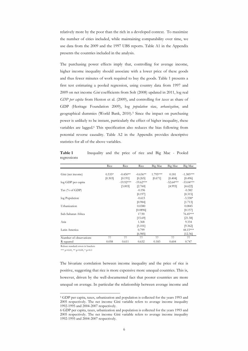
The purchasing power effects imply that, controlling for average income,

higher income inequality should associate with a lower price of these goods

and thus fewer minutes of work required to buy the goods. Table 1 presents a

first test estimating a pooled regression, using country data from 1997 and

2009 on net income Gini coefficients from Solt (2008) updated in 2011, log real

GDP per capita from Heston et al. (2009), and controlling for taxes as share of

GDP (Heritage Foundation 2009), log population size, urbanization, and

geographical dummies (World Bank, 2010).5 Since the impact on purchasing

power is unlikely to be instant, particularly the effect of higher inequality, these

variables are lagged.6 This specification also reduces the bias following from

potential reverse causality. Table A2 in the Appendix provides descriptive

statistics for all of the above variables.

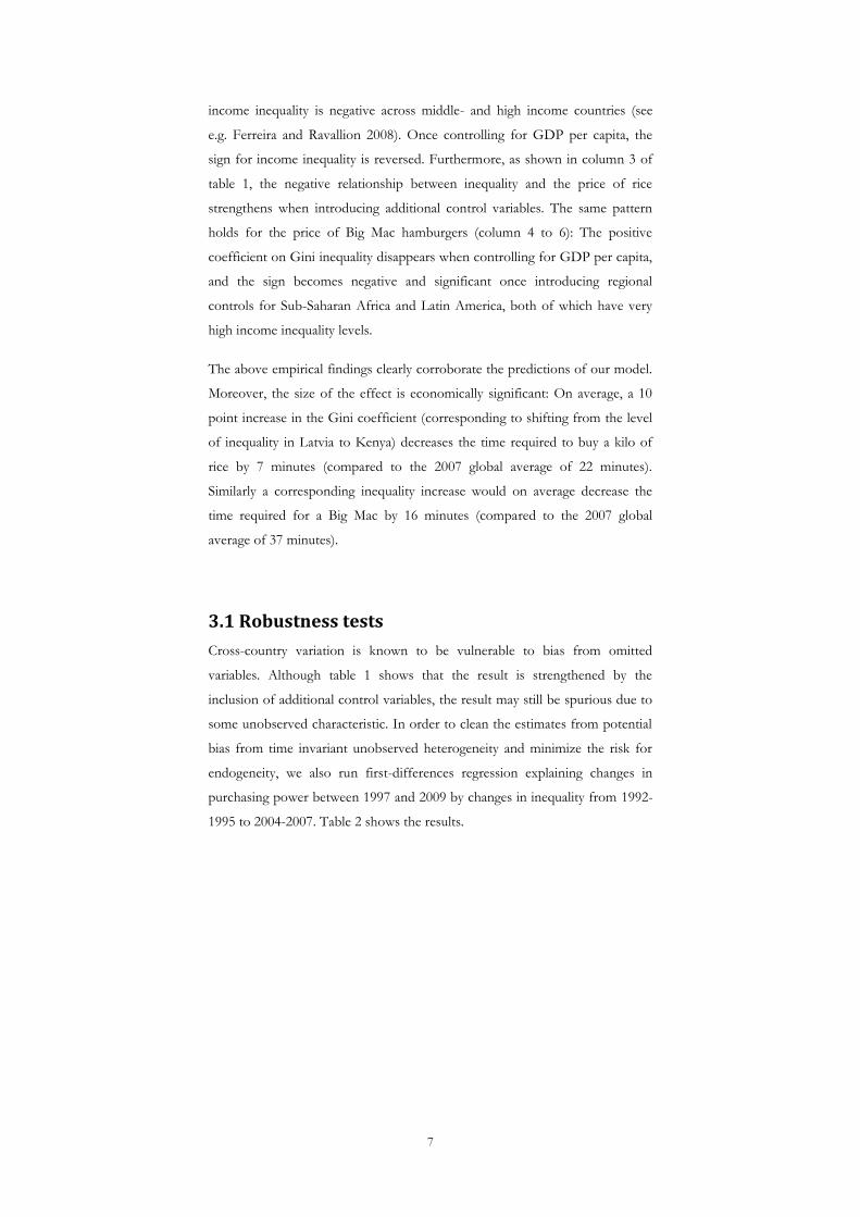
Table 1 Inequality and the price of rice and Big Mac - Pooled regressions

The bivariate correlation between income inequality and the price of rice is

positive, suggesting that rice is more expensive more unequal countries. This is,

however, driven by the well-documented fact that poorer countries are more

unequal on average. In particular the relationship between average income and

5 GDP per capita, taxes, urbanization and population is collected for the years 1993 and 2005 respectively. The net income Gini variable refers to average income inequality 1992-1995 and 2004-2007 respectively. 6 GDP per capita, taxes, urbanization and population is collected for the years 1993 and 2005 respectively. The net income Gini variable refers to average income inequality 1992-1995 and 2004-2007 respectively.

Rice Rice Rice Big Mac Big Mac Big Mac

Gini (net income) 0.535* -0.450** -0.636** 1.795*** 0.181 -1.385***

[0.303] [0.191] [0.265] [0.671] [0.404] [0.496]

log GDP per capita -19.92*** -19.62*** -32.64*** -33.04***

[3.003] [2.760] [4.993] [4.622]

Tax (% of GDP) -0.196 -0.382

[0.197] [0.315]

log Population -0.615 -3.338*

[0.984] [1.713]

Urbanization 0.0380 0.0845

[0.0896] [0.157]

Sub-Saharan Africa 17.90 76.45***

[15.69] [21.58]

Asia 1.368 9.334

[5.101] [9.362]

Latin America 0.799 44.15***

[6.985] [12.36]

Number of observations 77 77 77 77 77 77

R-squared 0.058 0.611 0.632 0.183 0.604 0.747

Robust standard errors in brackets

*** p<0.01, ** p<0.05, * p<0.1

7

income inequality is negative across middle- and high income countries (see

e.g. Ferreira and Ravallion 2008). Once controlling for GDP per capita, the

sign for income inequality is reversed. Furthermore, as shown in column 3 of

table 1, the negative relationship between inequality and the price of rice

strengthens when introducing additional control variables. The same pattern

holds for the price of Big Mac hamburgers (column 4 to 6): The positive

coefficient on Gini inequality disappears when controlling for GDP per capita,

and the sign becomes negative and significant once introducing regional

controls for Sub-Saharan Africa and Latin America, both of which have very

high income inequality levels.

The above empirical findings clearly corroborate the predictions of our model.

Moreover, the size of the effect is economically significant: On average, a 10

point increase in the Gini coefficient (corresponding to shifting from the level

of inequality in Latvia to Kenya) decreases the time required to buy a kilo of

rice by 7 minutes (compared to the 2007 global average of 22 minutes).

Similarly a corresponding inequality increase would on average decrease the

time required for a Big Mac by 16 minutes (compared to the 2007 global

average of 37 minutes).

3.1 Robustness tests

Cross-country variation is known to be vulnerable to bias from omitted

variables. Although table 1 shows that the result is strengthened by the

inclusion of additional control variables, the result may still be spurious due to

some unobserved characteristic. In order to clean the estimates from potential

bias from time invariant unobserved heterogeneity and minimize the risk for

endogeneity, we also run first-differences regression explaining changes in

purchasing power between 1997 and 2009 by changes in inequality from 1992-

1995 to 2004-2007. Table 2 shows the results.

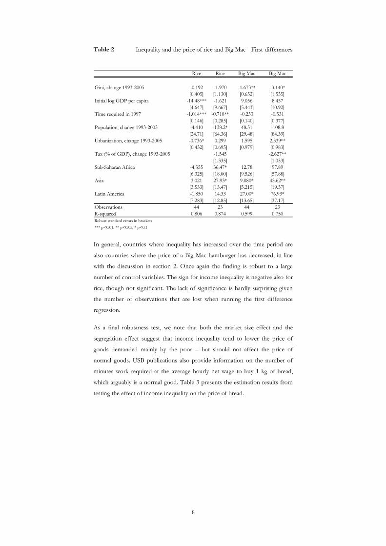
8

Table 2 Inequality and the price of rice and Big Mac - First-differences

In general, countries where inequality has increased over the time period are

also countries where the price of a Big Mac hamburger has decreased, in line

with the discussion in section 2. Once again the finding is robust to a large

number of control variables. The sign for income inequality is negative also for

rice, though not significant. The lack of significance is hardly surprising given

the number of observations that are lost when running the first difference

regression.

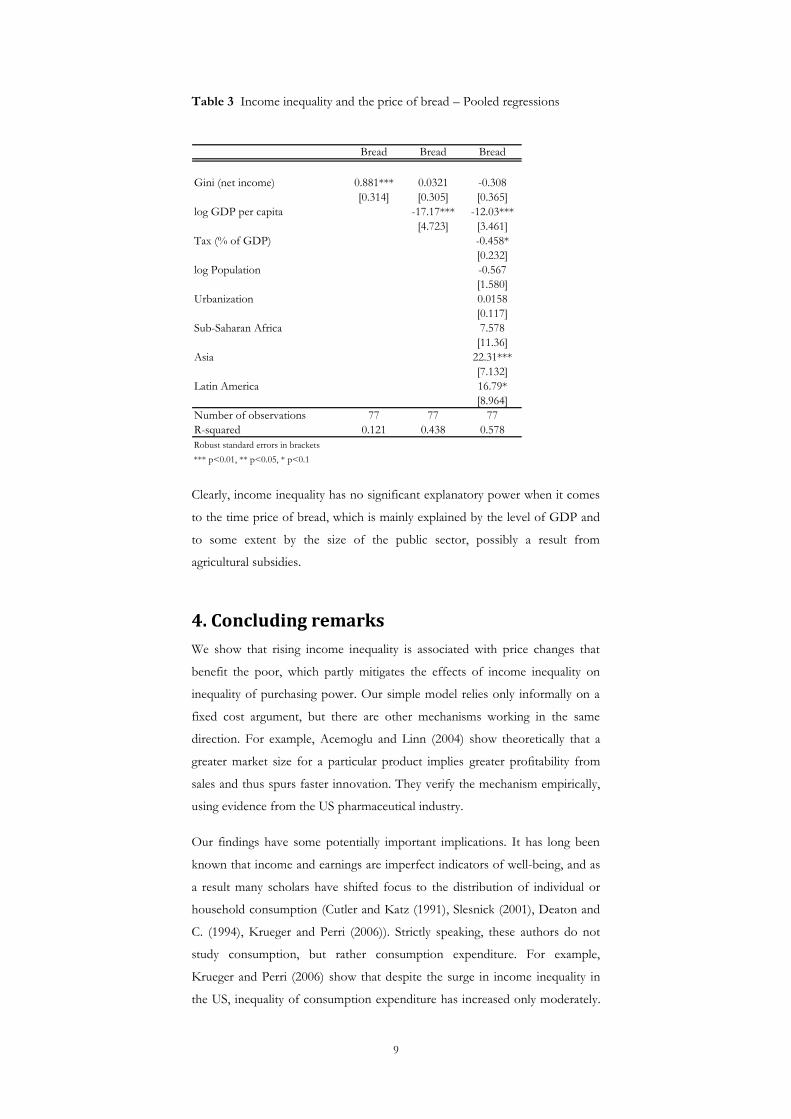
As a final robustness test, we note that both the market size effect and the

segregation effect suggest that income inequality tend to lower the price of

goods demanded mainly by the poor – but should not affect the price of

normal goods. USB publications also provide information on the number of

minutes work required at the average hourly net wage to buy 1 kg of bread,

which arguably is a normal good. Table 3 presents the estimation results from

testing the effect of income inequality on the price of bread.

Rice Rice Big Mac Big Mac

Gini, change 1993-2005 -0.192 -1.970 -1.673** -3.140*

[0.405] [1.130] [0.652] [1.555]

Initial log GDP per capita -14.48*** -1.621 9.056 8.457

[4.647] [9.667] [5.443] [10.92]

Time required in 1997 -1.014*** -0.718** -0.233 -0.531

[0.146] [0.285] [0.140] [0.377]

Population, change 1993-2005 -4.410 -138.2* 48.51 -108.8

[24.71] [64.36] [29.48] [84.39]

Urbanization, change 1993-2005 -0.736* 0.299 1.595 2.339**

[0.432] [0.695] [0.979] [0.983]

Tax (% of GDP), change 1993-2005 -1.545 -2.627**

[1.335] [1.053]

Sub-Saharan Africa -4.355 36.47* 12.78 97.89

[6.325] [18.00] [9.526] [57.88]

Asia 3.021 27.93* 9.080* 43.62**

[3.533] [13.47] [5.215] [19.57]

Latin America -1.850 14.33 27.00* 76.93*

[7.283] [12.85] [13.65] [37.17]

Observations 44 23 44 23

R-squared 0.806 0.874 0.599 0.750

Robust standard errors in brackets

*** p<0.01, ** p<0.05, * p<0.1

9

Table 3 Income inequality and the price of bread – Pooled regressions

Clearly, income inequality has no significant explanatory power when it comes

to the time price of bread, which is mainly explained by the level of GDP and

to some extent by the size of the public sector, possibly a result from

agricultural subsidies.

4. Concluding remarks

We show that rising income inequality is associated with price changes that

benefit the poor, which partly mitigates the effects of income inequality on

inequality of purchasing power. Our simple model relies only informally on a

fixed cost argument, but there are other mechanisms working in the same

direction. For example, Acemoglu and Linn (2004) show theoretically that a

greater market size for a particular product implies greater profitability from

sales and thus spurs faster innovation. They verify the mechanism empirically,

using evidence from the US pharmaceutical industry.

Our findings have some potentially important implications. It has long been

known that income and earnings are imperfect indicators of well-being, and as

a result many scholars have shifted focus to the distribution of individual or

household consumption (Cutler and Katz (1991), Slesnick (2001), Deaton and

C. (1994), Krueger and Perri (2006)). Strictly speaking, these authors do not

study consumption, but rather consumption expenditure. For example,

Krueger and Perri (2006) show that despite the surge in income inequality in

the US, inequality of consumption expenditure has increased only moderately.

Bread Bread Bread

Gini (net income) 0.881*** 0.0321 -0.308

[0.314] [0.305] [0.365]

log GDP per capita -17.17*** -12.03***

[4.723] [3.461]

Tax (% of GDP) -0.458*

[0.232]

log Population -0.567

[1.580]

Urbanization 0.0158

[0.117]

Sub-Saharan Africa 7.578

[11.36]

Asia 22.31***

[7.132]

Latin America 16.79*

[8.964]

Number of observations 77 77 77

R-squared 0.121 0.438 0.578

Robust standard errors in brackets

*** p<0.01, ** p<0.05, * p<0.1

10

Our study suggests that the well-being of the poor may be even better than

suggested by their results, as the purchasing power of a given level of

consumption expenditure increases due to price changes.

It remains to be explored if purchasing power effects are large enough to have

substantial consequences for the welfare of the poor. In this context, our

results are relevant for the large literature on the health effects of income

inequality, where results are currently very mixed – as shown by overviews by

Subramanian and Kawachi (2004) and Kondo, et al. (2009). For example,

psychological health measures may be more sensitive to the income

distribution while more physiological measures are likely to also depend on the

distribution of purchasing power.

Finally, it should be noted that the above analysis has disseminated the

relationship between inequality and purchasing power focusing on inferior and

normal goods. As discussed by Veblen (1994 [1899]) it is however likely that

purchasing power effects do not generally benefit the poor (∂Pp/∂λ > 0) when

it comes to status goods and conspicuous consumption. For example, when

there is limited supply of attractively located housing demanded by both rich

and poor, higher income of the rich will increase the price of these goods and

thus decrease the purchasing power of the poor.

In any case, our study highlights a very general point. When examining

economic well-being, it is important to analyze not only the incomes or even

expenditure of households, but also the prices of the products they buy.

Acknowledgements We are thankful for comments and suggestions from

participants in the 2010 American Public Choice Meeting (Monterey, CA), in

the 2011 ECINEQ meeting in Italy, and in the Department of Economics

seminar series of Umeå University, Lund University and the Ratio institute. We

are also sincerely thankful for comments from Niclas Berggren, and the help

and work done by research assistant Ingrid Magnusson. This work is partially

funded by the Swedish International Development Cooperation Agency

Sida/SAREC.

11

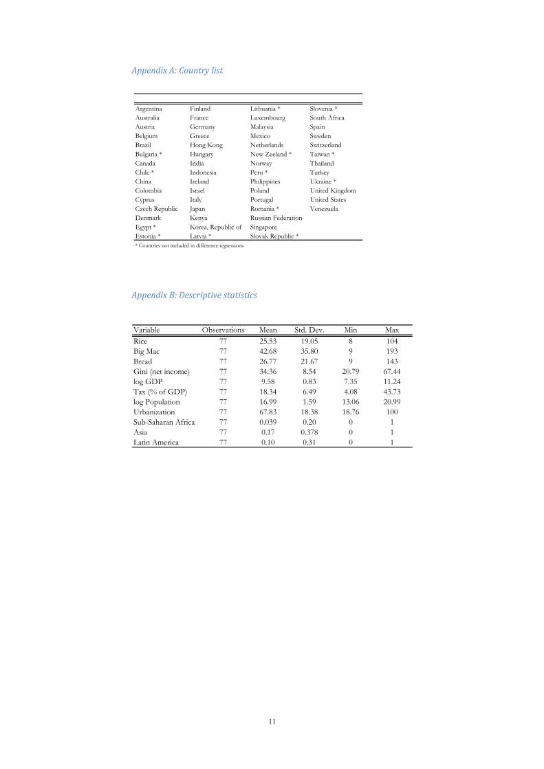
Appendix A: Country list

Appendix B: Descriptive statistics

Argentina Finland Lithuania * Slovenia *

Australia France Luxembourg South Africa

Austria Germany Malaysia Spain

Belgium Greece Mexico Sweden

Brazil Hong Kong Netherlands Switzerland

Bulgaria * Hungary New Zeeland * Taiwan *

Canada India Norway Thailand

Chile * Indonesia Peru * Turkey

China Ireland Philippines Ukraine *

Colombia Israel Poland United Kingdom

Cyprus Italy Portugal United States

Czech Republic Japan Romania * Venezuela

Denmark Kenya Russian Federation

Egypt * Korea, Republic of Singapore

Estonia * Latvia * Slovak Republic *

* Countries not included in difference regressions

Variable Observations Mean Std. Dev. Min Max

Rice 77 25.53 19.05 8 104

Big Mac 77 42.68 35.80 9 193

Bread 77 26.77 21.67 9 143

Gini (net income) 77 34.36 8.54 20.79 67.44

log GDP 77 9.58 0.83 7.35 11.24

Tax (% of GDP) 77 18.34 6.49 4.08 43.73

log Population 77 16.99 1.59 13.06 20.99

Urbanization 77 67.83 18.38 18.76 100

Sub-Saharan Africa 77 0.039 0.20 0 1

Asia 77 0.17 0.378 0 1

Latin America 77 0.10 0.31 0 1

12

References

Acemoglu, D., and Linn, J. (2004). Market Size in Innovation: Theory and

Evidence from the Pharmaceutical Industry. Quarterly Journal of

Economics, 119, 1049-1090.

Anderson, J., and Billou, N. (2007). Serving the World’s Poor: innovation at

the base of the economic pyramid. Journal of Business Strategy.

Broda, C., and Romalis, J. (2009). The Welfare Implications of Rising Price

Dispersion. Mimeo.

Cutler, D., and Katz, L. (1991). Rising Inequality? Changes in the Distribution

of Income and Consumption in the 1980s. American Economic Review,

82, 546–551.

Deaton, A., and C., P. (1994). Intertemporal Choice and Inequality. Journal of

Political Economy, 102, 437–467.

Kondo, N., Sembajwe, G., Kawachi, I., van Dam Rob, M., Subramanian, S.V.,

and Yamagata, Z. (2009). Income inequality, mortality, and self rated

health: meta-analysis of multilevel studies. 339, b4471-b4471.

Krueger, D., and Perri, F. (2006). Does Income Inequality Lead to

Consumption Inequality? Evidence and Theory. Review of Economic

Studies, 73, 163-93.

Lambert, P.J. (1993). The Distribution and Redistribution of Income. New York:

Manchester University Press.

Pendakur, K. (2002). Taking prices seriously in the measurement of inequality.

Journal of Public Economics, 86, 47-69.

Slesnick, D.T. (2001). Consumption and Social Welfare: Living Standards and Their

Distribution in the United States. Cambridge: Cambridge University

Press.

Solt, F. (2008). Standardizing the World Income Inequality Database. Social

Science Quarterly, 90, 231-242.

Subramanian, S.V., and Kawachi, I. (2004). Income Inequality and Health:

What Have We Learned So Far? Epidemiologic Reviews, 26, 78-91.

Weatherspoon, D.D., and Reardon, T. (2003). The Rise of Supermarkets in

Africa: Implications for Agrifood Systems and the Rural Poor

Development Policy Review, 21.

Veblen, T. (1994 [1899]). The Theory of the Leisure Class. New York.: Dover.

(orig. publ. by Macmillan, NY).