when ‘false’ models predict better than ‘true’ ones...
TRANSCRIPT

When ‘false’ models predict better than ‘true’ ones:Paradoxes of the bias-variance tradeoff
Hemank Lamba <[email protected]>
Momin M. Malik <[email protected]>
10-702/36-702: Statistical Machine LearningThursday, May 4, 2017
Introduction
The paradox
Lasso
Bias-variancetradeoff
Conclusion
References
Prediction vs. explanation
• Classical statistics focused on inference and unbiased estimators
• Why? Wanted explanations of or information about underlyingdata-generating processes
• ML focuses on prediction. A separate goal (Shmueli, 2010; Breiman,2001), often with very different methods
• But... why should prediction be different? How can a model that predictsbetter be further from the ‘truth’?
10702: StatML Paradoxes of the bias-variance tradeoff 1 of 14 Hemank Lamba & Momin Malik

Introduction
The paradox
Lasso
Bias-variancetradeoff
Conclusion
References
A ‘false’ model that predicts better than a ‘true’ one
• All models are ‘wrong’ (Box, 1979), usually because we haven’t or can’tmeasure all causal variables or we have the wrong function class
• If we have all causal variables and the right function class, then a ‘false’model is one with the wrong variables (“misspecified”) (and/or withincorrect estimates/inferences)
• Can a ‘wrong’ model predict better? Yes.
10702: StatML Paradoxes of the bias-variance tradeoff 2 of 14 Hemank Lamba & Momin Malik

Introduction
The paradox
Lasso
Bias-variancetradeoff
Conclusion
References
A ‘false’ model that predicts better than a ‘true’ one
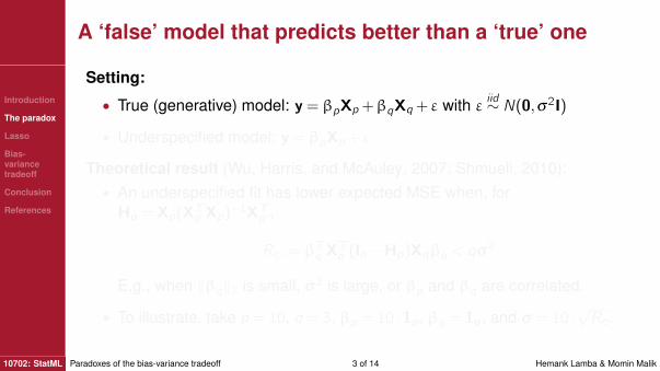
Setting:
• True (generative) model: y = βpXp+βqXq+ε with ε iid∼ N(0,σ2I)
• Underspecified model: y = βpXp+ε
Theoretical result (Wu, Harris, and McAuley, 2007; Shmueli, 2010):• An underspecified fit has lower expected MSE when, forHp = Xp(X
Tp Xp)
−1XTp ,
Rc := βTq XTq (In−Hp)Xqβq < qσ
2
E.g., when ‖βq‖1 is small, σ2 is large, or βp and βq are correlated.
• To illustrate, take p = 10, q = 3, βp = 10 ·1p, βq = 1q, and σ = 10 ·√Rc .
10702: StatML Paradoxes of the bias-variance tradeoff 3 of 14 Hemank Lamba & Momin Malik
Introduction
The paradox
Lasso
Bias-variancetradeoff
Conclusion
References
A ‘false’ model that predicts better than a ‘true’ one
Setting:
• True (generative) model: y = βpXp+βqXq+ε with ε iid∼ N(0,σ2I)
• Underspecified model: y = βpXp+ε
Theoretical result (Wu, Harris, and McAuley, 2007; Shmueli, 2010):• An underspecified fit has lower expected MSE when, forHp = Xp(X
Tp Xp)
−1XTp ,
Rc := βTq XTq (In−Hp)Xqβq < qσ
2
E.g., when ‖βq‖1 is small, σ2 is large, or βp and βq are correlated.
• To illustrate, take p = 10, q = 3, βp = 10 ·1p, βq = 1q, and σ = 10 ·√Rc .
10702: StatML Paradoxes of the bias-variance tradeoff 3 of 14 Hemank Lamba & Momin Malik

Introduction
The paradox
Lasso
Bias-variancetradeoff
Conclusion
References
A ‘false’ model that predicts better than a ‘true’ one
Generate X= (Xp,Xq) so Xq is correlated with q features in Xp.
X1
X2
X3
X4
X5
X6
X7
X8
X9
X10
X11
X12
X13
10702: StatML Paradoxes of the bias-variance tradeoff 4 of 14 Hemank Lamba & Momin Malik

Introduction
The paradox
Lasso
Bias-variancetradeoff
Conclusion
References
A ‘false’ model that predicts better than a ‘true’ oneGenerate X= (Xp,Xq) so Xq is correlated with q features in Xp.
X1
X2
X3
X4
X5
X6
X7
X8
X9
X10
X11
X12
X13
10702: StatML Paradoxes of the bias-variance tradeoff 4 of 14 Hemank Lamba & Momin Malik

Introduction
The paradox
Lasso
Bias-variancetradeoff
Conclusion
References
A ‘false’ model that predicts better than a ‘true’ one
0.0 0.5 1.0 1.5 2.0 2.5 3.0
0.0
0.2
0.4
0.6
0.8
1.0
MSE of true vs. underspecified over 5000 runs
MSE
Den
sity
TrueUnderspecified
10702: StatML Paradoxes of the bias-variance tradeoff 5 of 14 Hemank Lamba & Momin Malik

Introduction
The paradox
Lasso
Bias-variancetradeoff
Conclusion
References
Selection approach
• In practice, would probably use the lasso, not hand-pick features. Whatdoes the lasso give?
• Note: consistency of the lasso is investigated versus the oracle predictor(minimizer of L0 penalty), not the ‘truth’
• Conditions involve restrictions on the design matrix (van de Geer andBuhlmann, 2009), which our matrix fails (we think)
10702: StatML Paradoxes of the bias-variance tradeoff 6 of 14 Hemank Lamba & Momin Malik

Introduction
The paradox
Lasso
Bias-variancetradeoff
Conclusion
References
Selection approach
0.0 0.5 1.0 1.5 2.0 2.5 3.0
0.0
0.2
0.4
0.6
0.8
1.0
1.2
MSE of true, underspecified, and lasso over 5000 runs
MSE
Den
sity
TrueUnderspecifiedLasso
10702: StatML Paradoxes of the bias-variance tradeoff 7 of 14 Hemank Lamba & Momin Malik

Introduction
The paradox
Lasso
Bias-variancetradeoff
Conclusion
References
Selection approachInterestingly, the λ that is optimal over a validation set always selects out theintercept. Result: neither the true nor the underspecified model!
X1 X2 X3 X4 X5 X6 X7 X8 X9 X10 X11 X12 X13
Fraction of times feature selectedout by lasso over 5000 runs
0.0
0.2
0.4
0.6
0.8
1.0
10702: StatML Paradoxes of the bias-variance tradeoff 8 of 14 Hemank Lamba & Momin Malik

Introduction
The paradox
Lasso
Bias-variancetradeoff
Conclusion
References
Bias-variance tradeoff
• The underspecified model and the lasso decrease prediction error versus‘truth’ by decreasing the variance
• I.e., the bias-variance tradeoff can explain any disconnect between‘prediction’ and ‘truth’
• But, bias-variance decomposition is specific to L2 loss. Does it generalizeto arbitrary loss functions?
• No. (Only to strictly convex)
10702: StatML Paradoxes of the bias-variance tradeoff 9 of 14 Hemank Lamba & Momin Malik

Introduction
The paradox
Lasso
Bias-variancetradeoff
Conclusion
References
Generalizing the bias-variance tradeoff
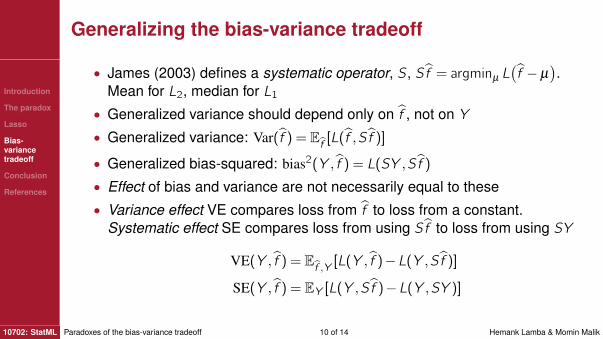
• James (2003) defines a systematic operator, S , Sf = argminµ L(f −µ
).
Mean for L2, median for L1• Generalized variance should depend only on f , not on Y
• Generalized variance: Var(f ) = Ef[L(f ,Sf )]
• Generalized bias-squared: bias2(Y , f ) = L(SY ,Sf )
• Effect of bias and variance are not necessarily equal to these
• Variance effect VE compares loss from f to loss from a constant.Systematic effect SE compares loss from using Sf to loss from using SY
VE(Y , f ) = Ef ,Y
[L(Y , f )−L(Y ,Sf )]
SE(Y , f ) = EY [L(Y ,Sf )−L(Y ,SY )]
10702: StatML Paradoxes of the bias-variance tradeoff 10 of 14 Hemank Lamba & Momin Malik

Introduction
The paradox
Lasso
Bias-variancetradeoff
Conclusion
References
Generalizing the bias-variance tradeoff
• James (2003) defines a systematic operator, S , Sf = argminµ L(f −µ
).
Mean for L2, median for L1• Generalized variance should depend only on f , not on Y
• Generalized variance: Var(f ) = Ef[L(f ,Sf )]
• Generalized bias-squared: bias2(Y , f ) = L(SY ,Sf )
• Effect of bias and variance are not necessarily equal to these
• Variance effect VE compares loss from f to loss from a constant.Systematic effect SE compares loss from using Sf to loss from using SY
VE(Y , f ) = Ef ,Y
[L(Y , f )−L(Y ,Sf )]
SE(Y , f ) = EY [L(Y ,Sf )−L(Y ,SY )]
10702: StatML Paradoxes of the bias-variance tradeoff 10 of 14 Hemank Lamba & Momin Malik

Introduction
The paradox
Lasso
Bias-variancetradeoff
Conclusion
References
Applying to 0-1 loss
• Say we have a trained classifier where for some level X = x , we haveP(Y |X = x) = (0.5,0.4,0.1)
• Bayes (optimal) classifier is f ∗(x) = (1,0,0)
• Say that f is not smooth, such that f doesn’t manage to be Bayes at x
• Consider two biased classifiers, f1(x) = (0,1,0) and f2(x) = (0,0,1) bothwith a ‘bias’ of 1, and zero variance
• What if we randomize the predictions? P(f1(x)|X = x) = (0.4,0.5,0.1) andP(f2(x)|X = x) = (0.1,0.5,0.4). Both have the same distribution ofprobabilities, so, the same variance
10702: StatML Paradoxes of the bias-variance tradeoff 11 of 14 Hemank Lamba & Momin Malik

Introduction
The paradox
Lasso
Bias-variancetradeoff
Conclusion
References
Applying to 0-1 loss
• For 0-1 loss,
VE(Y , f ) = Ef ,Y
[L(Y , f )−L(Y ,Sf )] = Ef ,Y
[I (Y 6= f )− I (Y 6= Sf )]
= P(Y 6= f )−P(Y 6= Sf ) =(1−∑
ki=1πi πi
)−(1−πargmaxi πi
)= πargmaxi πi
−∑ki=1πi πi
• Then,
VE(f1,Y ) = 0.4− (0.5 ·0.4+0.4 ·0.5+0.1 ·0.1) = .40−0.41= −0.01
VE(f2,Y ) = 0.4− (0.5 ·0.1+0.4 ·0.5+0.1 ·0.4) = .40−0.29= 0.11
• The same amount of variance can increase or decrease the expectedaccuracy, completely separate from the bias!
10702: StatML Paradoxes of the bias-variance tradeoff 12 of 14 Hemank Lamba & Momin Malik

Introduction
The paradox
Lasso
Bias-variancetradeoff
Conclusion
References
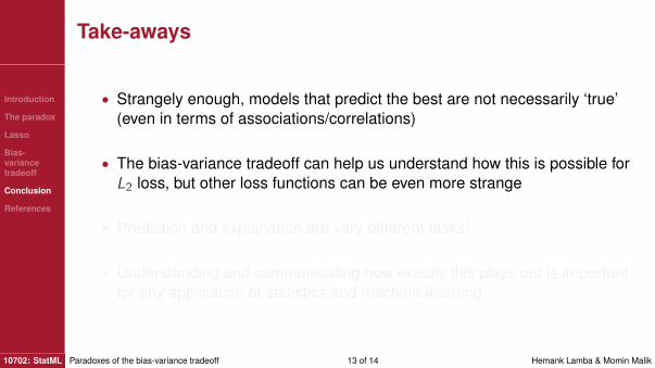
Take-aways
• Strangely enough, models that predict the best are not necessarily ‘true’(even in terms of associations/correlations)
• The bias-variance tradeoff can help us understand how this is possible forL2 loss, but other loss functions can be even more strange
• Prediction and explanation are very different tasks!
• Understanding and communicating how exactly this plays out is importantfor any application of statistics and machine learning
10702: StatML Paradoxes of the bias-variance tradeoff 13 of 14 Hemank Lamba & Momin Malik

Introduction
The paradox
Lasso
Bias-variancetradeoff
Conclusion
References
Take-aways
• Strangely enough, models that predict the best are not necessarily ‘true’(even in terms of associations/correlations)
• The bias-variance tradeoff can help us understand how this is possible forL2 loss, but other loss functions can be even more strange
• Prediction and explanation are very different tasks!
• Understanding and communicating how exactly this plays out is importantfor any application of statistics and machine learning
10702: StatML Paradoxes of the bias-variance tradeoff 13 of 14 Hemank Lamba & Momin Malik

Introduction
The paradox
Lasso
Bias-variancetradeoff
Conclusion
References
References
Box, George E. P. (1979). Robustness in the strategy of scientific model building. Tech. rep.#1954. University of Madison-Wisconsin, Mathematics Research Center.
Breiman, Leo (2001). “Statistical modeling: The two cultures (with comments and a rejoinder bythe author)”. In: Statistical Science 16.3, pp. 199–231. DOI: 10.1214/ss/1009213726.
James, Gareth M. (2003). “Variance and bias for general loss functions”. In: Machine Learning51.2, pp. 115–135. DOI: 10.1023/A:1022899518027.
Shmueli, Galit (2010). “To explain or to predict?” In: Statistical Science 25.3, pp. 289–310. DOI:10.1214/10-STS330.
van de Geer, Sara A. and Peter Buhlmann (2009). “On the conditions used to prove oracleresults for the lasso”. In: Electronic Journal of Statistics 3, pp. 1360–1392. DOI:10.1214/09-EJS506.
Wu, Shaohua, T. J. Harris, and K. B. McAuley (2007). “The use of simplified or misspecifiedmodels: Linear case”. In: The Canadian Journal of Chemical Engineering 85.4,pp. 386–398. DOI: 10.1002/cjce.5450850401.
10702: StatML Paradoxes of the bias-variance tradeoff 14 of 14 Hemank Lamba & Momin Malik

Statistical Topological Data Analysis
Chaitanya Ahuja1
Bhuwan Dhingra1
1Language Technologies InstitureCarnegie Mellon University
C. Ahuja, B. Dhingra (LTI, CMU) Statistical TDA 1 / 14

Contents
1 Introduction – Topological Data Analysis
2 Density Trees
3 Statistical Inference over Trees
4 Visualization of Word Embeddings
C. Ahuja, B. Dhingra (LTI, CMU) Statistical TDA 2 / 14

Topological Data Analysis
Topological Data Analysis (TDA) refers to data analysis methodswhich study properties such as shape, topology and connectedness ofthe data.
This includes:
Clustering (particularly Density Based Clustering)Density Modes and Ridge EstimationManifold Learning / Dimension ReductionPersistent Homology
TDA is useful as a visualization tool and for summarizinghigh-dimensional datasets.
C. Ahuja, B. Dhingra (LTI, CMU) Statistical TDA 3 / 14
This Project
We review recent work [1] on performing statistical inference forDensity Trees—a particular class of hierarchical clustering methods.
Outline:
Definitions and Tree TopologyConstructing confidence sets via bootstrapPruning trees to remove insignificant features
As an application, we generate density trees to visualize distributionof words in documents
C. Ahuja, B. Dhingra (LTI, CMU) Statistical TDA 4 / 14

Density Trees
Suppose the data lies in X ⊂ Rd . Given a density functionf : X → [0,∞),
Let Tf (λ) denote the connected components of the upper level set{x : f (x) > λ}. These are the high density clusters at level λ.The density tree is the collection of all such clusters:{Tf } = Tf = ∪λTf (λ).This is a tree by construction, i.e. if A,B ∈ {Tf }, then either A ⊂ B,or B ⊂ A or A ∩ B = φ.
Figure: Obtained from [2]
C. Ahuja, B. Dhingra (LTI, CMU) Statistical TDA 5 / 14

Estimated Tree
In general we have an iid sample from the true density X1,X2, . . . ,XN ∼ p.The Estimated Tree Tph is the tree constructed from the Kernel DensityEstimate:
ph(x) =1
nhd
N∑i=1
K (‖x − Xi‖
h)
Tph(λ) = {x : ph(x) > λ}
C. Ahuja, B. Dhingra (LTI, CMU) Statistical TDA 6 / 14

Tree Topology
Given a tree {Tf }, we can define thetree distance function between elements of the tree:
dTf(C1,C2) = λ1 + λ2 − 2mf (C1,C2) C1,C2 ∈ {Tf }
It can be shown that dTfis a metric on {Tf }, and hence induces a
metric topology on it.
Lemma
If the true unknown density p is a morse function, then ∃ a constanth0 > 0, such that ∀h s.t. 0 < h ≤ h0, the true cluster tree, Tp and theestimated tree Tph have the same metric topology above.
Hence we do not need to let the KDE bandwidth h→ 0. This leads to adimension-independent rate of convergence for the bootstrap confidenceset.C. Ahuja, B. Dhingra (LTI, CMU) Statistical TDA 7 / 14

Confidence Sets via Bootstrap
To construct confidence sets, we first need a metric to measure the“closeness” of two trees. The l∞ metric is defined as,
d∞ (Tp,Tq) = supx∈χ|p(x)− q(x)| = ‖p − q‖∞
The confidence set is defined as Cα = {T : d∞(T ,Tph) ≤ tα} for Tph .
tα can be obtained by the bootstrap:
F (s) =1
B
B∑i=1
I(d∞(T iph,Tph) < s)
tα = F−1(1− α)
Where {T 1ph, . . . , TB
ph} are the estimated trees for the bootstrap
samples {X 11 , . . . , X
1n }, . . . , {XB
1 , . . . , XBn }.
C. Ahuja, B. Dhingra (LTI, CMU) Statistical TDA 8 / 14

Convergence Rate
Theorem
Under regularity conditions on the kernel, the constructed confidenceinterval is asymptotically valid and satisfies,
P(Tp ∈ Cα
)= 1− α + O
(log7 n
nhd
) 16
(1)
where Cα = {T : d∞(T ,Tph) ≤ tα}
From the Lemma presented previously, we can fix h to a small constant, to
obtain a dimension-independent rate of O(log7 nn
) 16.
C. Ahuja, B. Dhingra (LTI, CMU) Statistical TDA 9 / 14
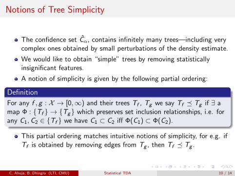
Notions of Tree Simplicity
The confidence set Cα, contains infinitely many trees—including verycomplex ones obtained by small perturbations of the density estimate.
We would like to obtain “simple” trees by removing statisticallyinsignificant features.
A notion of simplicity is given by the following partial ordering:
Definition
For any f , g : X → [0,∞) and their trees Tf , Tg we say Tf � Tg if ∃ amap Φ : {Tf } → {Tg} which preserves set inclusion relationships, i.e. forany C1,C2 ∈ {Tf } we have C1 ⊂ C2 iff Φ(C1) ⊂ Φ(C2).
This partial ordering matches intuitive notions of simplicity, for e.g. ifTf is obtained by removing edges from Tg , then Tf � Tg .
C. Ahuja, B. Dhingra (LTI, CMU) Statistical TDA 10 / 14

Pruning Rules
Following two strategies are suggested to prune the empirical tree Tph :
1 Pruning leaves: Remove all leaves of the tree with length less than2tα.
2 Pruning leaves and internal branches: Remove all leaves andinternal branches of the tree with cumulative length less than 2tα.
It can be shown that the tree obtained after pruning from either of thesetwo strategies,
Is simpler than Tph .
Is generated from a valid density function.
And the density function lies in the constructed confidence set.
C. Ahuja, B. Dhingra (LTI, CMU) Statistical TDA 11 / 14

Visualization of Word Embeddings
Figure: Cluster tree for Wikipedia Page on Noam Chomsky
C. Ahuja, B. Dhingra (LTI, CMU) Statistical TDA 12 / 14

Visualization of Word Embeddings
Figure: Cluster tree for Wikipedia Page on Leonardo da Vinci
C. Ahuja, B. Dhingra (LTI, CMU) Statistical TDA 13 / 14

References I
Jisu Kim et al. “Statistical Inference for Cluster Trees”. In: arXivpreprint arXiv:1605.06416 (2016).
Larry Wasserman. “Topological Data Analysis”. In: arXiv preprintarXiv:1609.08227 (2016).
C. Ahuja, B. Dhingra (LTI, CMU) Statistical TDA 14 / 14

PCA-Based estimation for functional linear regressionwith functional responses
Ruixi Fan Shuo Zhao
Carnegie Mellon University, Pittsburgh, PA
CCML, 2017
Ruixi Fan, Shuo Zhao (Carnegie Mellon University)PCA-Based estimation for functional linear regression with functional responsesCCML, 2017 1 / 37

Outline
1 IntroductionFunctional data analysis (FDA)Functional linear regression & MotivationFunctional Principal Component Analysis(FPCA)Problem statement
2 Proof of convergence ratesDivide the problemBound the error termsMinimax rate
Ruixi Fan, Shuo Zhao (Carnegie Mellon University)PCA-Based estimation for functional linear regression with functional responsesCCML, 2017 2 / 37

Outline
1 IntroductionFunctional data analysis (FDA)Functional linear regression & MotivationFunctional Principal Component Analysis(FPCA)Problem statement
2 Proof of convergence ratesDivide the problemBound the error termsMinimax rate
Ruixi Fan, Shuo Zhao (Carnegie Mellon University)PCA-Based estimation for functional linear regression with functional responsesCCML, 2017 3 / 37

Functional data analysis (FDA)
Functional Data (FD) refer to data recorded during a time interval orintermittently at several discrete time points.
Functional Data Analysis (FDA) deals with FD for classification,clustering, regression etc. In FDA, each sample element is consideredto be a function over time, spatial location, wavelength, probabilityand so on.
Applications: time series, images, shapes, or more general objects.
Ruixi Fan, Shuo Zhao (Carnegie Mellon University)PCA-Based estimation for functional linear regression with functional responsesCCML, 2017 4 / 37

Outline
1 IntroductionFunctional data analysis (FDA)Functional linear regression & MotivationFunctional Principal Component Analysis(FPCA)Problem statement
2 Proof of convergence ratesDivide the problemBound the error termsMinimax rate
Ruixi Fan, Shuo Zhao (Carnegie Mellon University)PCA-Based estimation for functional linear regression with functional responsesCCML, 2017 5 / 37

Motivation
Functional predictor regression
Functional response regression
Function-on-function regression
Estimation of the coefficient function
Optimal convergence rate
Ruixi Fan, Shuo Zhao (Carnegie Mellon University)PCA-Based estimation for functional linear regression with functional responsesCCML, 2017 6 / 37

Outline
1 IntroductionFunctional data analysis (FDA)Functional linear regression & MotivationFunctional Principal Component Analysis(FPCA)Problem statement
2 Proof of convergence ratesDivide the problemBound the error termsMinimax rate
Ruixi Fan, Shuo Zhao (Carnegie Mellon University)PCA-Based estimation for functional linear regression with functional responsesCCML, 2017 7 / 37

Functional Principal Component Analysis(FPCA)
Covariance function
K (s, t) = Cov{X (s),X (t)}
Spectral expansion of covariance
According to the Hilbert-Schmidt theorem,
K (s, t) =∞∑k=1
κkφk(s)φk(t)
where κ1 ≥ κ2 ≥ ... > 0. It has
Ruixi Fan, Shuo Zhao (Carnegie Mellon University)PCA-Based estimation for functional linear regression with functional responsesCCML, 2017 8 / 37

Functional Principal Component Analysis(FPCA)
Spectral expansion and FPCA
X (t) = µX (t) +∞∑k=1
ξkφk(t)
where all the coefficients are listed in the order: ξ1 > ξ2 > ... > 0, thentruncate at k = m,
X (t) ≈ Xm(t) = µX (t) +m∑
k=1
ξkφk(t)
Ruixi Fan, Shuo Zhao (Carnegie Mellon University)PCA-Based estimation for functional linear regression with functional responsesCCML, 2017 9 / 37

Outline
1 IntroductionFunctional data analysis (FDA)Functional linear regression & MotivationFunctional Principal Component Analysis(FPCA)Problem statement
2 Proof of convergence ratesDivide the problemBound the error termsMinimax rate
Ruixi Fan, Shuo Zhao (Carnegie Mellon University)PCA-Based estimation for functional linear regression with functional responsesCCML, 2017 10 / 37

Functional linear regression
Functional linear regression
Y (s) = µY (s) +
∫Ib(s, t)[X (t)− µX (t)]dt + ε(t)
where I = [0, 1].
Regression model by expectation
E (Y |X )(s) = µY (s) +
∫Ib(s, t)[X (t)− µX (t)]dt
where E (Y |X ) is the conditional expectation of Y as an L2(I )-valuedrandom variable conditionally on the σ-field generated by X.
Ruixi Fan, Shuo Zhao (Carnegie Mellon University)PCA-Based estimation for functional linear regression with functional responsesCCML, 2017 11 / 37

Formulation of estimator
Single Truncation estimator
b(s, t) =mn∑k=1
1
κk(
1
n
∑ξi ,kYi (s))φk(t)
where K (s, t) is estimated in the emprical covariance function:ˆK (s, t) = 1
n
∑ni=1(Xi (s)− X (s))(Xi (t)− X (t)).
Expand K (s, t) with eigenvalue {κk}∞k=1 and eigenfunctions {φk}∞k=1.
ξi ,k = infI{Xi (t)− X (t)}φk(t)dt
Ruixi Fan, Shuo Zhao (Carnegie Mellon University)PCA-Based estimation for functional linear regression with functional responsesCCML, 2017 12 / 37

Convergence rates
General Assumptions
∃ α > 1, β > 1.5, γ > 0.5,C1 > 0 st
E [||X ||2] <∞,E [||Y ||2|X ] ≤ C1a.s.; E [ξ4k ] ≤ C1κ
2k ,∀k ≥ 1;
κk ≤ C1k−α, κk − κk+1 ≥ C−1
1 k−α−1,∀k ≥ 1;
|bj ,k | ≤ C1j−γk−β, ∀j , k ≥ 1, β >
α
2+ 1;
Convergence rate of Single truncation
∃ α > 1, β > 1.5, γ > 0.5,C1 > 0, choose mn such thatmn = o(n1/(2α+2)), then
|||b − b|||2 = Op(n−(2β−1)/(α+2β))
Ruixi Fan, Shuo Zhao (Carnegie Mellon University)PCA-Based estimation for functional linear regression with functional responsesCCML, 2017 13 / 37

Outline
1 IntroductionFunctional data analysis (FDA)Functional linear regression & MotivationFunctional Principal Component Analysis(FPCA)Problem statement
2 Proof of convergence ratesDivide the problemBound the error termsMinimax rate
Ruixi Fan, Shuo Zhao (Carnegie Mellon University)PCA-Based estimation for functional linear regression with functional responsesCCML, 2017 14 / 37

Some important expansions
On {φj ⊗ φk}∞j ,k=1, expand b and b:
b =∑j ,k
bj ,k(φj ⊗ φk)
b =∞∑j=1
mn∑k=1
bj ,k(φj ⊗ φk)
Note: φj ⊗ φk ≡ φj(s)φk(t), bj ,k =n−1
∑ni=1 ηi,j ξi,kκk
,
bj ,k =∫∫
b(s, t)(φj ⊗ φk), bj ,k =∫ ∫
I 2 b(s, t)(φj ⊗ φk)
Set ηci ,j = ηi ,j −∑n
k=1 ηk,jn and εci ,j = εi ,j −
∑nk=1 εk,jn ,
⇒ ηci ,j =∑
l bj ,l ξi ,l + εci ,j .
⇒ bj ,k =1
κk(
1
n
n∑i=1
∑l
bj ,l ξi ,l ξi ,k+1
n
n∑i=1
εi ,j ξi ,k) = bj ,k+1
κk(
1
n
n∑i=1
εi ,j ξi ,k)
.
⇒ (bj ,k − bj ,k)2 . (bj ,k − bj ,k)2 +1
κ2k
(1
n
n∑i=1
εi ,j ξi ,k)2Ruixi Fan, Shuo Zhao (Carnegie Mellon University)PCA-Based estimation for functional linear regression with functional responsesCCML, 2017 15 / 37
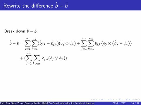
Rewrite the difference b − b
Break down b − b:
b − b =∞∑j=1
mn∑k=1
(bj ,k − bj ,k)(φj ⊗ φk) +∞∑j=1
mn∑k=1
bj ,k{φj ⊗ (φk − φk)}
+ (∞∑j=1
∑k>mn
bj ,k(φj ⊗ φk))
Ruixi Fan, Shuo Zhao (Carnegie Mellon University)PCA-Based estimation for functional linear regression with functional responsesCCML, 2017 16 / 37

Rewrite |||b − b|||2
|||b − b|||2 .∞∑j=1
mn∑k=1
(bj ,k − bj ,k)2 +
∫∫{∞∑j=1
mn∑k=1
bj ,k{φj ⊗ (φk − φk)}}2
+∞∑j=1
∑k>mn
b2j ,k
.∞∑j=1
mn∑k=1
1
κ2k
(1
n
n∑i=1
εi ,j ξi ,k)2
︸ ︷︷ ︸eigenvalue error
+∞∑j=1
mn∑k=1
(bj ,k − bj ,k)2
︸ ︷︷ ︸coefficient error
+
∫∫{∞∑j=1
mn∑k=1
bj ,k{φj ⊗ (φk − φk)}}2
︸ ︷︷ ︸basis error
+∞∑j=1
∑k>mn
b2j ,k︸ ︷︷ ︸
higher-order term
Ruixi Fan, Shuo Zhao (Carnegie Mellon University)PCA-Based estimation for functional linear regression with functional responsesCCML, 2017 17 / 37
Outline
1 IntroductionFunctional data analysis (FDA)Functional linear regression & MotivationFunctional Principal Component Analysis(FPCA)Problem statement
2 Proof of convergence ratesDivide the problemBound the error termsMinimax rate
Ruixi Fan, Shuo Zhao (Carnegie Mellon University)PCA-Based estimation for functional linear regression with functional responsesCCML, 2017 18 / 37
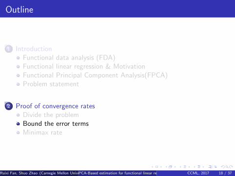
Bound the eigenvalue error
To bound∑∞
j=1
∑mnk=1
1κ2k
( 1n
∑ni=1 εi ,j ξi ,k)2, we have
|κk/κk − 1| . kα|κk − κk | . mαn |||K − K ||| = Op(1)
Since εi ,j are independent with mean zero conditionally onX n
1 = {X1, ...,Xn}, we get
E [(1
n
n∑i=1
εi ,j ξi ,k)2|X n1 ] =
1
n2
n∑i=1
E [ε2i ,j |X n
1 ]ξ2i ,k
With Bessel’s inequality :∑∞j=1 E [ε2
i ,j |X n1 ] = E [
∑∞j=1 ε
2i ,j |X n
1 ] ≤ E [||Ei ||2|X n1 ] ≤ C1, we have
E [∞∑j=1
mn∑k=1
1
κ2k
(1
n
n∑i=1
εi ,j ξi ,k)2|X n1 ] .
1
n
mn∑k=1
1
κk= Op(n−1mα+1
n )
⇒∞∑j=1
mn∑k=1
1
κ2k
(1
n
n∑i=1
εi ,j ξi ,k)2 = Op(n−1mα+1n )
Ruixi Fan, Shuo Zhao (Carnegie Mellon University)PCA-Based estimation for functional linear regression with functional responsesCCML, 2017 19 / 37

Decompose the coefficient error
To bound∑∞
j=1
∑mnk=1(bj ,k − bj ,k)2, generally we assume that
inf l :l 6=k |κk − κl | > 0, then
φk − φk =∑
l :l 6=k(κk − κl)−1φl∫ ∫
(K − K )(φk ⊗ φl) + φk∫
(φk − φk)φk
bj ,k − bj ,k =∑l :l 6=k
bj ,l(κk − κl)−1
∫ ∫(K − K )(φk ⊗ φl)
+∑l :l 6=k
bj ,l{(κk − κl)−1 − (κk − κl)−1}∫ ∫
(K − K )(φk ⊗ φl)
+∑l :l 6=k
bj ,l(κk − κl)−1
∫ ∫(K − K )((φk − φk)⊗ φl)
+ bj ,k
∫(φk − φk)φk
:= Tj ,k,1 + Tj ,k,2 + Tj ,k,3 + Tj ,k,4
Ruixi Fan, Shuo Zhao (Carnegie Mellon University)PCA-Based estimation for functional linear regression with functional responsesCCML, 2017 20 / 37
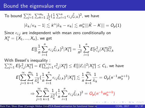
bound component Tj ,k ,4,Tj ,k ,3
It is clear that |Tj ,k,4| . j−γk−β||φk − φk ||.Since |
∫ ∫(K − K ){(φk − φk)⊗ φl}| ≤ |||K − K |||||φk − φk ||,
we will get the following:|Tj ,k,3| . j−γ |||K − K ||| · ||φk − φk ||
∑l :l 6=k
l−β
|κk−κl |
Ruixi Fan, Shuo Zhao (Carnegie Mellon University)PCA-Based estimation for functional linear regression with functional responsesCCML, 2017 21 / 37
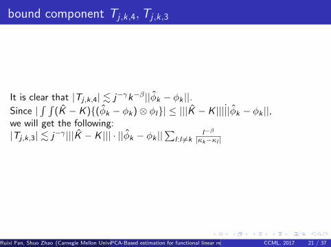
bound Tj ,k ,1
Based on the assumption that κk ' k−α, we can choose k ≥ 1 and C > 1large enough so that κk/κk/C ≤ 1/2 and κ[Ck]+1/κk ≤ 1/2,∀k ≥ k0,where [.] is a ceiling function. Now, we can partition the sum into three
parts:∑
l :l 6=k =∑[k/C ]
l=1 +∑[Ck]
l=[k/C ]+1 +∑∞
l=[Ck]+1
Through suitable estimation, we can get the following:
[k/C ]∑l=1
l−β
(κl − κk).
1, if β > α + 1
log k , if β = α + 1
kα−β+1, if β < α + 1
∞∑l=[Ck]+1
l−β
(κk − κl). kα−β+1
[Ck]∑[k/C ]+1
l−β
|κk − κl |.
{1, β > α + 1
kα−β+1 log k , β ≤ α + 1
⇒ E (T 2j ,k,1) . n−1j−2γk−α
Ruixi Fan, Shuo Zhao (Carnegie Mellon University)PCA-Based estimation for functional linear regression with functional responsesCCML, 2017 22 / 37

bound Tj ,k ,2
Define the event An:
An = {|κk − κl | ≥ |κk − κl |/2,∀k : 1 ≤ k ≤ mn,∀l 6= k}
On the event An,
|Tj ,k,2| . j−γ |||K − K |||∑l :l 6=k
l−β vk,l|κk − κl |2
where vk,l = | 1n∑n
i=1 ξi ,kξi ,l − ξk ξl |, then we have
E{(∑l :l 6=k
l−β
|κk − κl |2vk,l)
2} ≤ [(∑l :l 6=k
l−β
|κk − κl |2E{v2
k,l})1/2]2
. n−1k−α(∑l :l 6=k
l−β−α/2
|κk − κl |2)
Ruixi Fan, Shuo Zhao (Carnegie Mellon University)PCA-Based estimation for functional linear regression with functional responsesCCML, 2017 23 / 37

bound Tj ,k ,2
Using the same splitting trick in the Tj ,k,1 part, we can get
∑l :l 6=k
l−β−α/2
|κk − κl |2= (
[k/C ]∑l=1
+
[Ck]∑l=[k/C ]+1
+∞∑
l=[Ck]+1
)l−β−α/2
|κk − κl |2
.[k/C ]∑l=1
l3α/2−β + k2α+2
[Ck]∑l=[k/C ]+1
l−β−α/2
|k − l |2+
k2α∞∑
l=[Ck]+1
l−β−α/2
. 1 + k3α/2−β+1 log k + k3α/2−β+2 + k3α−β+1
. 1 + k3α/2−β+2
⇒ |Tj ,k,2| . n−1k2α−2β+4
Ruixi Fan, Shuo Zhao (Carnegie Mellon University)PCA-Based estimation for functional linear regression with functional responsesCCML, 2017 24 / 37

Summarize over Tj ,k ,1∼4, (bound coefficient error)
∞∑j=1
mn∑k=1
(T 2j ,k,1 + ...+ T 2
j ,k,4) = Op(n−1 + n−2{m3n + m2α−2β+5
n (logmn)2})
= Op(1
n)
Ruixi Fan, Shuo Zhao (Carnegie Mellon University)PCA-Based estimation for functional linear regression with functional responsesCCML, 2017 25 / 37

Bound the basis error
Using Parseval’s identity,∫∫{∞∑j=1
mn∑k=1
bj ,k{φj ⊗ (φk − φk)}}2 =∞∑j=1
∫{
mn∑k=1
bj ,k(φk − φk)}2
. mn
∞∑j=1
mn∑k=1
b2j ,k ||φk − φk ||2
. mn
mn∑k=1
k−2β||φk − φk ||2
= Op(n−1mn)
Ruixi Fan, Shuo Zhao (Carnegie Mellon University)PCA-Based estimation for functional linear regression with functional responsesCCML, 2017 26 / 37

bound the high-order term
And the square of L2-norm of the high-order term is:
(∞∑j=1
∑k>mn
bj ,k(φj ⊗ φk))2 =∞∑j=1
∑k>mn
b2j ,k = Op(m−2β+1
n )
(Orthogonality of the basis set)
Ruixi Fan, Shuo Zhao (Carnegie Mellon University)PCA-Based estimation for functional linear regression with functional responsesCCML, 2017 27 / 37

Put all four terms together
|||b − b|||2 .∞∑j=1
mn∑k=1
1
κ2k
(1
n
n∑i=1
εi ,j ξi ,k)2
︸ ︷︷ ︸eigenvalue error=Op(n−1mα+1
n ))
+∞∑j=1
mn∑k=1
(bj ,k − bj ,k)2
︸ ︷︷ ︸coefficient error=Op(n−1)
+
∫∫{∞∑j=1
mn∑k=1
bj ,k{φj ⊗ (φk − φk)}}2
︸ ︷︷ ︸basis error=Op(n−1mn)
+∞∑j=1
∑k>mn
b2j ,k︸ ︷︷ ︸
higher-order term=Op(m−2β+1n )
= Op(n−1mα+1n + m−2β+1
n )
Take mn ∼ n1/(α+2β), we have
|||b − b|||2 = Op(n−2β−1α+2β )
Ruixi Fan, Shuo Zhao (Carnegie Mellon University)PCA-Based estimation for functional linear regression with functional responsesCCML, 2017 28 / 37

Outline
1 IntroductionFunctional data analysis (FDA)Functional linear regression & MotivationFunctional Principal Component Analysis(FPCA)Problem statement
2 Proof of convergence ratesDivide the problemBound the error termsMinimax rate
Ruixi Fan, Shuo Zhao (Carnegie Mellon University)PCA-Based estimation for functional linear regression with functional responsesCCML, 2017 29 / 37

Minimax rate
Cameron-Martin space
Let Pb,x denote the distribution of∫I b(·, t)x(t)dt + ε(·), and P0 denote
the distribution of ε. Then the Cameron-Martin Space are defined as thefollowing:
H = {h =∑j
hjφj :∑j
h2j
λj<∞}
with the < h, g >H=∑
jhjgjλj, h =
∑j hjφj , g =
∑j gjφj
Ruixi Fan, Shuo Zhao (Carnegie Mellon University)PCA-Based estimation for functional linear regression with functional responsesCCML, 2017 30 / 37

Joint distribution of (X ,Y )
Then the probability density can be formulated by Cameron-Martinformula:
pb,x(y) =dPb,x
dP0(y) = exp{−
∑j
(∑
k bj ,kxk)2
2λj+
∑j
yj∑
k bj ,kxkλj
}
where y =∑
j yjφj .If we denote by Q the distribution of X, then the joint distribution of(X ,Y ) is given by pb,x(y)dP0(y)dQ(x)
Ruixi Fan, Shuo Zhao (Carnegie Mellon University)PCA-Based estimation for functional linear regression with functional responsesCCML, 2017 31 / 37

Estimation of distribution
Then let νn = [n1/(α+2β)], and
bθ =2νn∑νn+1
k−βθk−νn(φ1 ⊗ φk)
where θ ∈ {0, 1}νn , thus the probability density function is the following:
pbθ,x(y) = exp{−(∑2νn
k=νn+1 k−βθk−νnxn))2
2λ1+
y1∑2νn
k=νn+1 k−βθk=νnxk
λ1}
If we define pθ,x(y) = pbθ,x(y), then the estimated distribution ispθ,x(y)dP0(y)dQ(x) for each θ.Let (X1,Y1), ..., (Xn,Yn) be i.i.d from Pθ, then the estimator of bθ is:
bn =∑j ,k
bj ,k(φj ⊗ φk)
Ruixi Fan, Shuo Zhao (Carnegie Mellon University)PCA-Based estimation for functional linear regression with functional responsesCCML, 2017 32 / 37

Get the lower bound of |||bn − bθ|||2
∀θ, θ′ ∈ {0, 1}νn , let ρ(θ, θ′) =∑νn
k=1 |θk − θ′k | (Hamming distance), then
Pθ{|||bn − bθ|||2 ≥ (2νn)−2β
4c} ≥ Pθ{ρ(θn, θ) ≥ c}
According to Assouad’s Lemma, we have
maxθ
Eθ{ρ(θn, θ)} ≥ νn4e−1/2λ1
Then apply Paley-Zygmund inequality, we have
Pθ{|||bn − bθ|||2 ≥ (2νn)−2β
4
1
16e−1/(2λ1)} ≥ Pθ{ρ(θn, θ) ≥ νn
8e−1/(2λ1)}
≥ 1
16e−1/2λ1
Ruixi Fan, Shuo Zhao (Carnegie Mellon University)PCA-Based estimation for functional linear regression with functional responsesCCML, 2017 33 / 37

Get lower bound of |||bn − bθ|||2
Therefore
maxθ
Pθ{|||bn − bθ|||2 ≥ µ−2β+1n
2β + 5e−1/(2λ1)} ≥ 1
16e−1/(2λ1)
Notice that ν−2β+1n ∼ n−(2β−1)/(α+2β), then apply Chebyshev inequality,
we have the lower bound like that in the lecture note:
infbn
supθ
Eθ|||bn − bθ|||2 & n−2β−1α+2β
Ruixi Fan, Shuo Zhao (Carnegie Mellon University)PCA-Based estimation for functional linear regression with functional responsesCCML, 2017 34 / 37

Summary
Single Truncation estimator:
b(s, t) =mn∑k=1
1
κk(
1
n
∑ξi ,kYi (s))φk(t)
Covergence rate of ordinary least-square linear regression:||b − b||22 . σp(X )−1
√p/n.
Convergence rate of PCA-based functional linear regression:
|||b − b|||2 . Op(n−2β−1α+2β ).
Ruixi Fan, Shuo Zhao (Carnegie Mellon University)PCA-Based estimation for functional linear regression with functional responsesCCML, 2017 35 / 37

References I
M. Imaizumi, K. KatoPCA-based estimation for functional linear regression with functionalresponse.arxiv:1609.00286v2, 2016.
K. Han, H. ShinFunctional linear regression for functional response via sparse basisselectionJournal of the Korean Statistical Society, 44, 376-389, 2015
J. Wang, J. Chiou, H. Mueller,Review of Functional Data Analysis,arXiv:1507.05135, 2015
J. Morris,Functional Regression,arXiv:1406.4068, 2014
Ruixi Fan, Shuo Zhao (Carnegie Mellon University)PCA-Based estimation for functional linear regression with functional responsesCCML, 2017 36 / 37

References II
J. Ramsay, B. Silverman,Functional Data Analysis,Springer Series in Statistics Chapter 16, 2005
Ruixi Fan, Shuo Zhao (Carnegie Mellon University)PCA-Based estimation for functional linear regression with functional responsesCCML, 2017 37 / 37

Inference of Sparse Gaussian Graphical Models:
Algorithms and TheoryIfigeneia Apostolopoulou

Applications of Gaussian Graphical Models (GGM)
• Popular tool for learning network structure over a large number of continuous variables
• Neuroscience• Computational Biology• Natural Language Processing• Computational Finance• Energy Forecasting
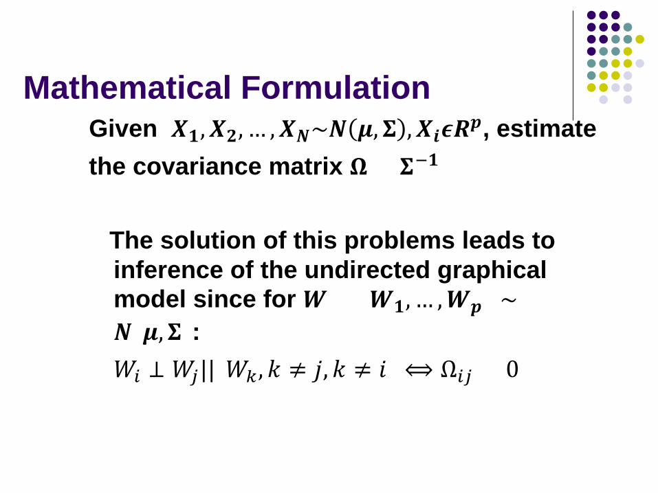
Mathematical Formulation Given 𝑿𝑿𝟏𝟏,𝑿𝑿𝟐𝟐, … ,𝑿𝑿𝑵𝑵~𝑵𝑵 𝝁𝝁,𝚺𝚺 ,𝑿𝑿𝒊𝒊𝝐𝝐𝑹𝑹𝒑𝒑, estimate the covariance matrix 𝛀𝛀 = 𝚺𝚺−𝟏𝟏
The solution of this problems leads to inference of the undirected graphical model since for 𝑾𝑾 = (𝑾𝑾𝟏𝟏, … ,𝑾𝑾𝒑𝒑) ∼𝑵𝑵(𝝁𝝁,𝚺𝚺):𝑊𝑊𝑖𝑖 ⊥ 𝑊𝑊𝑗𝑗||(𝑊𝑊𝑘𝑘,𝑘𝑘 ≠ 𝑗𝑗, 𝑘𝑘 ≠ 𝑖𝑖) ⟺ Ω𝑖𝑖𝑗𝑗 = 0
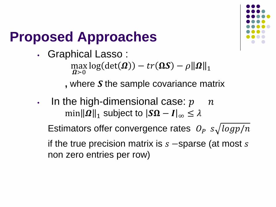
Proposed Approaches• Graphical Lasso :
max𝜴𝜴≻0
log det 𝜴𝜴 − 𝑡𝑡𝑡𝑡 𝛀𝛀𝛀𝛀 − 𝜌𝜌 𝜴𝜴 1
, where 𝛀𝛀 the sample covariance matrix
• In the high-dimensional case: 𝑝𝑝 > 𝑛𝑛min 𝜴𝜴 1 subject to 𝛀𝛀𝛀𝛀 − 𝑰𝑰 ∞ ≤ 𝜆𝜆
Estimators offer convergence rates 𝑂𝑂𝑃𝑃(𝑠𝑠 𝑙𝑙𝑙𝑙𝑙𝑙𝑝𝑝/𝑛𝑛)if the true precision matrix is 𝑠𝑠 −sparse (at most 𝑠𝑠non zero entries per row)

Conditional Gaussian Graphical Models
• Ignore correlations between input variables• 𝑿𝑿𝟏𝟏,𝑿𝑿𝟐𝟐, … ,𝑿𝑿𝑵𝑵,𝑿𝑿𝒊𝒊𝝐𝝐𝑹𝑹𝒑𝒑 the input variables,
𝒀𝒀𝟏𝟏,𝒀𝒀𝟐𝟐, … ,𝒀𝒀𝑵𝑵,𝒀𝒀𝒊𝒊𝝐𝝐𝑹𝑹𝒒𝒒 the output variables learn 𝜴𝜴𝒙𝒙𝒙𝒙,𝜴𝜴𝒙𝒙𝒙𝒙 such that
𝑝𝑝(𝒙𝒙|𝒙𝒙) ∼ 𝑁𝑁(−𝜴𝜴𝒙𝒙𝒙𝒙−1𝜴𝜴𝒙𝒙𝒙𝒙
𝑇𝑇 𝒙𝒙, 𝜴𝜴𝒙𝒙𝒙𝒙−1)
• This is a more detailed formulation of the multiple regression:𝒙𝒙 = 𝑩𝑩𝒙𝒙 + 𝝐𝝐

Proposed Approaches• Solution of the optimization problem:
• Second-order coordinate descent methods

Subspace ClusteringAlan Mishler & Deepika Bablani

Problem: Clustering is challenging in high dimensions
● Concentration of distance● Clusters may exist in different lower-dimensional spaces
Solution: Look for clusters in lower dimensional subspaces
● Bottom-up algorithms● Top-down algorithms● Model-based methods● Sparse subspace clustering
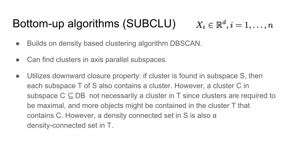
● Builds on density based clustering algorithm DBSCAN.
● Can find clusters in axis parallel subspaces.
● Utilizes downward closure property: if cluster is found in subspace S, then each subspace T of S also contains a cluster. However, a cluster C in subspace C DB not necessarily a cluster in T since clusters are required to be maximal, and more objects might be contained in the cluster T that contains C. However, a density connected set in S is also a density-connected set in T.
Bottom-up algorithms (SUBCLU)

Top-down algorithms (PROCLUS, ORCLUS)
PROCLUS (“PROJected CLUStering”)
● Goal: ○ Partition the data into clusters C1, C2, …, Ck, plus a set of outliers○ Partition the features into sets of dimensions D1, D2, …, Dk
corresponding to each cluster● Method: select k medoids, iteratively assign data points to clusters and
reduce dimensionality of each cluster
ORCLUS (“abitrarily ORiented projected CLUSter generation”)
● Extension of PROCLUS, looks for non-axis parallel subspaces.

Treat each data point as a linear combination of normally-distributed latent factors, plus normal noise. If Xi is in cluster g, then:
Model-based methods (EPGMMs)
matrix of factor weights
Estimate parameters using Alternating Expectation Conditional Maximization (AECM) algorithm
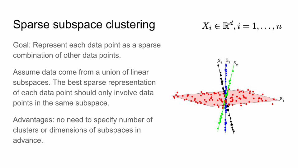
Sparse subspace clustering Goal: Represent each data point as a sparse combination of other data points.
Assume data come from a union of linear subspaces. The best sparse representation of each data point should only involve data points in the same subspace.
Advantages: no need to specify number of clusters or dimensions of subspaces in advance.

Conclusions
● Many different approaches● Since there’s no universal definition of cluster or a
subspace, there’s no “best” algorithm● Theoretical performance guarantees exist only for sparse
subspace clustering

Comparison of Dantizig Selector and Lasso
Xiaoyi Gu, Yufei Yi
May 2, 2017
Xiaoyi Gu, Yufei Yi
Comparison of Dantizig Selector and Lasso

Formulation
Goal
Under y ∈ Rn, X ∈ Rn×p with n� p, and z ∼ N (0, σ2I ) noise,want to estimate β ∈ Rp from
y = Xβ0 + z , (1)
Lasso
minβ‖y − Xβ‖`2 + λ‖β‖`1 . (2)
Dantizig Selector
minβ‖β‖`1 subject to ‖X ∗(y − Xβ)‖`∞ ≤ λpσ. (3)
Xiaoyi Gu, Yufei Yi
Comparison of Dantizig Selector and Lasso

Three Major Assumptions on X
UUP(Uniform Uncertainty Principle)
∃ S < p such that ∀|T | ≤ S , ∃δ such that for all c ∈ R|T |:(1− δ)‖c‖2`2 ≤ ‖XT c‖2`2 ≤ (1 + δ)‖c‖2`2
IDC(Incoherent Design Condition)
For β0 being Sn-sparse with limn→∞
Sn =∞. ∃en > 0 such that:
lim infn→∞enφmin(e
2nSn)
φmax (Sn+n) ≥ 18
MIC(Mutual Incoherent Condition)
ρ(S) = max{|〈Xi ,Xj〉| : i ∈ T , j ∈ T c , |T | ≤ S}. X satisfies MIC ifρ(S)S ≤ 1/K for some K > 0.
Xiaoyi Gu, Yufei Yi
Comparison of Dantizig Selector and Lasso

Comparison under the Restricted Eigenvalue Condition
REC(S , S ′,C0) Restricted Eigenvalue Condition
κ(S ,S ′,C0) := minT :|T |≤S
minc:‖cTc ‖`1≤C0‖cT∪R‖`1
‖Xc‖`2√n‖cT‖`1
> 0,
where R corresponds to the S ′ coordinates of |c| outside T .
Theorem [Bickel, Ritov,Tsybakov]
Suppose β0 is S-sparse and all diagonal elements of 1/n(X ∗X ) is 1,
Under RE(S , S ′, 1) and λp = σ√
log p/n,
‖βd − β0‖2`2 ≤ CS(1 +√
S/S ′)2σ2 log p
nκ4(S , S ′, 1)
Under RE(S , S ′, 3) and λ = σ√n · log p,
‖βl − β0‖2`2 ≤ C ′S(1 + 3√
S/S ′)2σ2 log p
nκ4(S , S ′, 3)
Xiaoyi Gu, Yufei Yi
Comparison of Dantizig Selector and Lasso

Statistical Analysis of Random Forests
Ritesh Noothigattu, Ben Parr

Breiman (2001)
● Formally defines a random forest
● Main results○ No overfitting as more trees are added○ Error depends on:
■ Individual tree strength■ Correlation between trees

Biau (2012), Denil et al (2014)
● Biau (2012)○ Consistency on a previously proposed variant○ Convergence rate depends only on number of strong features
● Denil et al (2014)○ A new theoretically tractable variant○ Proves consistency

Mix-membership ClusteringBoyan Duan, Xiaoyi Yang
Traditional Methods:-- Graph Representation
Node 2
Node 1
Node 4
Node 6
Node 5
Node 3
(1,2)
(1,4) (1,3)
(3,4)
(3,6)(3,5)
(5,6)

Traditional Methods:-- Extend Traditional K-means (NEO K-Means)
1. Traditional K-means Assignment matrix 𝑌𝑖𝑗Constrain: 𝑡𝑟𝑎𝑐𝑒(𝑈𝑇𝑈) = 𝑛, Row sum of 𝑌 is 1 vector.
2. NEO K-means Assignment matrix 𝑈𝑖𝑗Constrain: 𝑡𝑟𝑎𝑐𝑒(𝑈𝑇𝑈) = 1 + 𝛼 𝑛, Row sum of 𝑈 ≤ 𝛽𝑛.
3. Replace Y in the objective function of K-means into U.

Clustering based on motif network
Motif network
13
2

Clustering based on motif network
Motif network
13
24
56
78

Clustering based on motif network
Motif network
13
24
56
78
S
S

Clustering based on motif network
Motif network
13
24
56
78
Objective:
cut(Sj , Sj)
min(vol(Sj), vol(Sj))minS1,··· ,Sk
kX
j=1
degree of overlapping
s.t.
kX
j=1
#{nodes 2 Sj} (1 + ↵)n
S
S
Mathematical guarantee:Spectral graph methodology for weighted graph

Thank you!

Efficient PAC Reinforcement Learning in Contextual
Decision ProcessesKaran Goel
Deepak Dilipkumar

Problem Statement
• PAC Reinforcement Learning: Learn a near-optimal policy with high probability in sample efficient way
• Reinforcement Learning v/s Supervised Learning: Samples not iid

Contextual Decision Process• A recent general framework to model the world in
Krishnamurthy et al. (2016)
• Subsumes Markov Decision Processes, Partially Observable Markov Decision Processes
Bellman Rank of a CDP• New measure by Jiang et al. (2016) that characterizes
the complexity of a CDP
• Most practical problems actually have low Bellman rank

Main Paper• Jiang et al. (2016): Can learn policy for CDP with
low Bellman Rank with high sample efficiency
• Algorithm that outputs a near optimal policy with high probability given CDP with low Bellman Rank

Thanks!

Online Non-stationary Time Series Regression with Autoregressive Models
Lisheng Gao, Rui Peng

Motivation
• Problem Definition- Time Series: sequence of observations indexed in order (normally chronological)
- Stationarity: finite variation, constant first moment and second moment across time
- Online Optimization: iterative parameter tuning, incomplete knowledge of the future
• Why Important?- Natural temporal ordering
- Extremely wide applications (signal processing, weather forecasting, mathematical finance...)
• Connection with this course
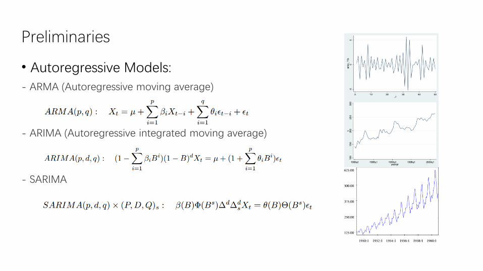
Preliminaries
• Autoregressive Models:- ARMA (Autoregressive moving average)
- ARIMA (Autoregressive integrated moving average)
- SARIMA

Theories – ARMA online gradient descent
• Loss –
• Regret –
[1]

Theories – generalized online gradient descent [2]
• Loss –

Theory – theoretical bound

• [1] Oren Anava, Elad Hazan, Shie Mannor, and Ohad Shamir. Online learning for time series prediction. arXiv preprint arXiv:1302.6927, 2013.
• [2] Christopher Xie, Avleen Bijral, and Juan Lavista Ferres. An online prediction framework for non-stationary time series. arXiv preprint arXiv:1611.02365, 2016.
References

Learning Sequential Data:
Hidden Markov Models and
BeyondSiqi Chen
10702 Project Presentation
CMU

Motivation
For many application such as speech recognition, bioinformatics musical
score following and stock prediction, the time series nature of the data is
intrinsic, so the usual i.i.d. assumption is no longer appropriate
HMM is a prototypical methods for modeling times series
However, it faces several important restrictions:
1. The number of hidden states is finite
2. If we have large number of possible states, then standard HMM may require
learning too many parameters.
3. Maximum likelihood estimation procedures do not consider the complexity
of the model, making it hard to avoid over or underfitting

Motivation
So we consider the following extensions of HMM:
Factorial HMM
Switiching State Space Models
Infinite Hidden Markov Model
To effectively discuss iHMM, need to consider Hierarchical Dirichlet Process
This brings the problem of inference algorithms:
Variational Learning for Switching State Space Models
Beam Sampling for Infinite Hidden Markov Models

Connection with class
An in-depth study of some particular instances (HMM and its extensions) of
dynamic Bayesian network and graphical model
Hierarchical Dirichlet process (HDP) can be used for clustering
By placing HMM in the general graphical model framework, the extensions and
inference algorithms become natural

Literature
Matthew J. Beal, Zoubin Ghahramani, and C. E. Rasmussen. The infinite hidden markovmodel.Neural Information Processing Systems, 14:577–585, 2002.
Z. Ghahramani and G. E. Hinton. Variational learning for switching state-space models. Neural Computation, 12(4):831–864, April 2000. ISSN 0899-7667.
Zoubin Ghahramani. An introduction to hidden markov models and bayesian networks. International Journal of Pattern Recognition and Artificial Intelligence, 15:9 – 42, 2001.
Michael Jordan. Graphical models. Statistical Science, Vol. 19:140 – 155, 2004.
Yee Whye Teh, Michael I Jordan, Matthew J Beal, and David M Blei. Hierarchical dirichletprocesses.Journal of the American Statistical Association, 101(476):1566–1581, 2006.
Jurgen Van Gael, Yunus Saatci, Yee Whye Teh, and Zoubin Ghahramani. Beam sampling for the
infinite hidden markov model. In Proceedings of the 25th international conference on Machine learning, pages 1088–1095. ACM, 2008.

HMM
(i) 𝑌𝑡 is generated by a process whose state 𝑆𝑡 is hidden from the observer.
(ii) 𝑆𝑡 has the Markov property: E[f(𝑆𝑡)|𝐹𝑠] = E[f(𝑆𝑡)|𝑆𝑠]
(iii) 𝑆𝑡 is discrete: 𝑆𝑡 can take K values {1,…,K}
The model:

Factorial HMM

Factorial HMM

Switching State Space Models

DP,HDP

iHMM The Infinite Hidden Markov Model (iHMM), is a non-parametric Bayesian extension of the
Hidden Markov Models with a infinite number of hidden states.
While in principle this will require the state transition matrix have infinite number of
parameters to estimate, the theory of Dirichlet Processes (DPs) enables us to implicitly
integrate the parameters out, leaving only a few hyperparameters defining the prior
HMM involves not a single mixture model, but rather a set of mixture models—one for
each value of the current state.
The current state 𝑆𝑡 indexes a specific row of the transition matrix, with the
probabilities in this row serving as the mixing proportions for the choice of the next state 𝑆𝑡+1
Thus, to consider a nonparametric variant of the HMM that allows a countable number of
states, we must consider a set of DPs, one for each value of the current state. Moreover,
these DPs must be linked, because we want the same set of next states to be reachable
from each of the current states
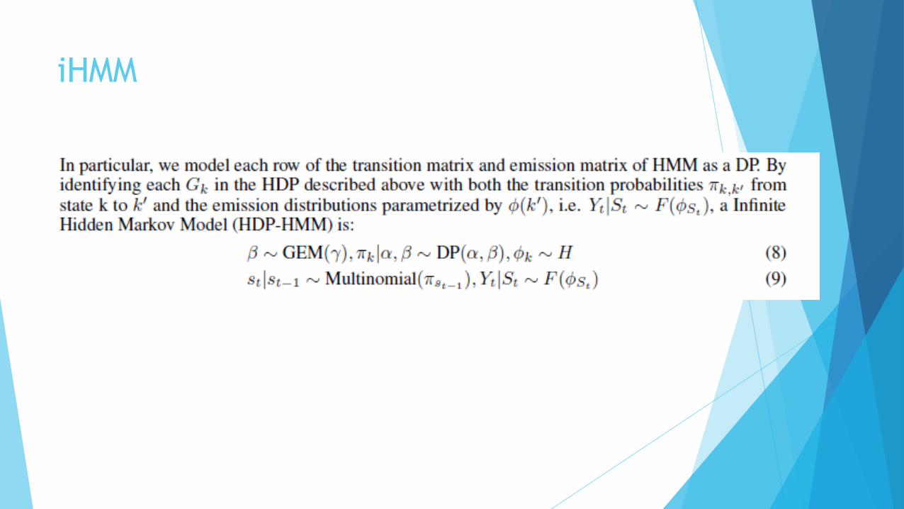
iHMM

iHMM
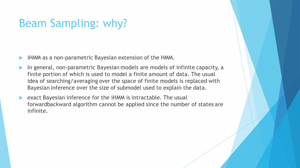
Beam Sampling: why?
iHMM as a non-parametric Bayesian extension of the HMM.
In general, non-parametric Bayesian models are models of infinite capacity, a
finite portion of which is used to model a finite amount of data. The usual
idea of searching/averaging over the space of finite models is replaced with
Bayesian inference over the size of submodel used to explain the data.
exact Bayesian inference for the iHMM is intractable. The usual
forwardbackward algorithm cannot be applied since the number of states are infinite.

Beam Sampling: idea
Beam sampling combines the idea of slice sampling and dynamic
programming.
The idea of beam sampling is to introduce auxiliary variables u such that
conditioned on u the number of trajectories with positive probability is finite.
We then apply dynamic programming to compute the conditional probabilities
of these trajectories and thus sample whole trajectories efficiently.
Note that the marginal distribution of other variables is not changed by the
introduced auxiliary variable U.

Thank you!


Gradient descent:
Key idea: natural gradient descent (NGD)

Gradient descent:
Newton method:
Key idea: natural gradient descent (NGD)

Gradient descent:
Newton method:
Natural gradient:
Key idea: natural gradient descent (NGD)
if

Gradient descent:
Newton method:
Natural gradient:
Key idea: natural gradient descent (NGD)
like Newton method for optimization of probability densities
if

Natural gradient:
How to approximate NGD?

Natural gradient:
How to approximate NGD?
Explicitly approximating and inverting 𝐹𝐹(𝜃𝜃𝑘𝑘)

Natural gradient:
How to approximate NGD?
Explicitly approximating and inverting 𝐹𝐹(𝜃𝜃𝑘𝑘)
• Cholesky factorization [Groose et al, 2015]

Natural gradient:
How to approximate NGD?
Explicitly approximating and inverting 𝐹𝐹(𝜃𝜃𝑘𝑘)
• Cholesky factorization [Groose et al, 2015]
• Kronecker factored approximation [Martens et al, 2015]
• …

Natural gradient:
How to approximate NGD?
Explicitly approximating and inverting 𝐹𝐹(𝜃𝜃𝑘𝑘)
• Cholesky factorization [Groose et al, 2015]
• Kronecker factored approximation [Martens et al, 2015]
• …
Change features or parameters so that 𝐹𝐹 𝜃𝜃𝑘𝑘 ≈ 𝐼𝐼

Natural gradient:
How to approximate NGD?
Explicitly approximating and inverting 𝐹𝐹(𝜃𝜃𝑘𝑘)
• Cholesky factorization [Groose et al, 2015]
• Kronecker factored approximation [Martens et al, 2015]
• …
Change features or parameters so that 𝐹𝐹 𝜃𝜃𝑘𝑘 ≈ 𝐼𝐼
• Normalization of input [LeCun et al, 1991]

Natural gradient:
How to approximate NGD?
Explicitly approximating and inverting 𝐹𝐹(𝜃𝜃𝑘𝑘)
• Cholesky factorization [Groose et al, 2015]
• Kronecker factored approximation [Martens et al, 2015]
• …
Change features or parameters so that 𝐹𝐹 𝜃𝜃𝑘𝑘 ≈ 𝐼𝐼
• Normalization of input [LeCun et al, 1991]
• Batch normalization [Ioffe et al, 2015]
• Weight normalization [Salimans et al, 2015]
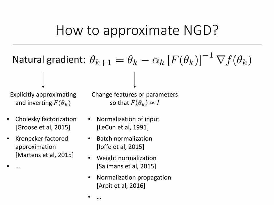
• Normalization propagation [Arpit et al, 2016]
• …
Other connections
• AdaGrad as approximation to NGD [Wager et al, 2013]
• Dropout as 𝐿𝐿2regularization in the Fisher space [Wager et al, 2013]
• …
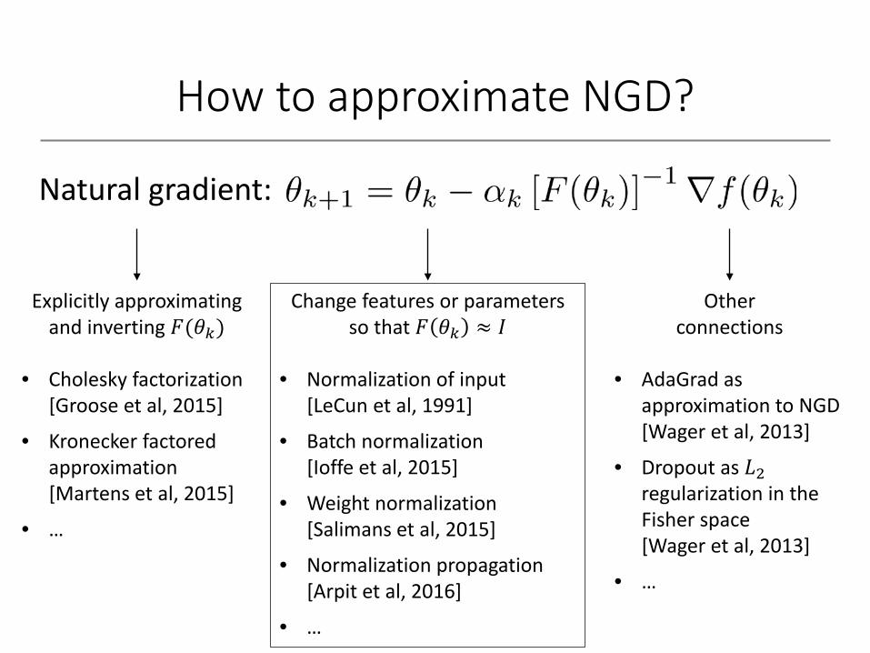

Variable Selection in High Dimensional FeatureSpace
A combination of Sure Independence Screening (SIS) andSmoothly Clipped Absolute Deviation (SCAD) method
Biwei Huang1 Xiongtao Ruan2
1Department of Philosophy
2Department of Computational BiologySchool of Computer Science
May 4th, 2017

Problem setting and SIS
I Problem: y = Xβ + ε, where y, ε ∈ Rn, X ∈ Rn×p, β ∈ Rp
I Aim: select o(n) variables from ultra-high dimensional feature
space (p = O(enξ), for ξ > 0).
I Two steps: 1. use SIS to reduce the dimensions to d = Θ(n);2. use SCAD method to further reduce the dimensions.
I SIS is based on correlation learning: ω = XTy .I Mγ = {1 ≤ i ≤ p : |ωi | is among the first [γn] largest of all},
where γ ∈ (0, 1), [γn] means the integer part of γn.
I Main property: Under regularity condition with sparsityassumption, SIS is accurate with high probability:
P(M∗ ⊂Mγ) = 1− O[exp{−Cn1−2κ/ log(n)}]
where M∗ is the true model, C > 0, and κ ∈ (0, 12) is aparameter.

SCAD
I Problem: ‖ y − Xβ ‖22 /2 +∑d
j=1 pλj (βj).
I The SCAD penalty is defined as
pλ(|β|) =
{ λ|β| if 0 ≤ |β| ≤ λ;
− |β|2−2aλ|β|+λ22(a−1) if λ ≤ |β| ≤ aλ;
(a + 1)λ2/2 if |β| ≥ aλ,
for some a > 2.
I With SCAD penalty, the estimator has three properties:sparsity, unbiasedness, and continuity.
I The estimator is root-n consistent (Op(n−1/2)) if λj → 0 forall j .
I The estimator has oracle properties. And SIS-SCAD also hasoracle properties

Reference
Fan, Jianqing and Lv, Jinchi, “Sure independence screeningfor ultrahigh dimensional feature space”, Journal of the RoyalStatistical Society: Series B (Statistical Methodology), 2008;70(5), pp. 849–911.Fan, Jianqing and Li, Runze, “Variable selection vianonconcave penalized likelihood and its oracle properties”, Journalof the American statistical Association, 2001; 96(456),pp. 1348–1360.Fan, Jianqing and Song, Rui and others, “Sure independencescreening in generalized linear models with NP-dimensionality”,The Annals of Statistics, 2010; 38(6), pp. 3567–3604.

Tuning parameter selection in high dimensional
variables selection tasks
Yu Chen, Haohan Wang

Challenges Solutions
some tuning parameter has unknown components
Tuning insensitive or tuning free approaches:
TIGER, Square-Root Lass, B-TREX
data dimension d is scaled with data sample size n Extended information criteria

CONSISTENCY AND CONVERGENCE RATES OF
GAUSSIAN RBF KERNEL SVMS
XIAOQI CHAI, JIAMING CAO

GAUSSIAN RBF KERNEL SVMS
• Training Data
• Gaussian RBF Kernel
• SVM as an optimization problem

CONSISTENCY

CONSISTENCY
Comments• Gaussian RBF kernel is a universal kernel — linear combinations of this kernel can approximate any
continuous function on the input space.• When using Gaussian RBF kernel, we can choose 𝛼𝛼 = 𝑑𝑑.• Gaussian RBF kernel SVMs are universally consistent with appropriate choice of the parameter λ.• But there does not exist a universal convergence rate for all probability.

PROBABILITY ASSUMPTIONS
Comments• They both describe noise near the decision boundary.• They can be related by the envelope order of the probability.

CONVERGENCE RATE 1
Comment• Under conditions of 𝛼𝛼 → ∞ and 𝑞𝑞 → ∞, optimal rate can be achieved, which approaches 𝑂𝑂(1
𝑛𝑛).

CONVERGENCE RATE 2
Comments• This rate is derived under more general condition
• The best rate it can achieve is 𝑂𝑂(𝑛𝑛−4𝛽𝛽(𝑞𝑞+1)
(2𝑞𝑞+𝑝𝑝𝑞𝑞+4)(1+𝛽𝛽))

DISCUSSION
• Gaussian RBF kernel SVMs are universally consistent;
• and have optimal fast convergence rate 𝑂𝑂(1𝑛𝑛
) under some assumptions,
• which restrict the noisiness of the data-generating distribution near the decision boundary.
• More general convergences rates in report

Learning withConditional Random Fields (CRF)
Chia-Yin ShihLiang-Kang Huang

Brief introduction of CRF
• Brief intro: a discriminative learning framework encoded with undirected PGM
• Motivation: Allows for more realistic modeling of NLP and image recognition tasks
• 702 Topics: Probabilistic graphical model, Reproducing Kernel Hilbert Space, MLE/MAP
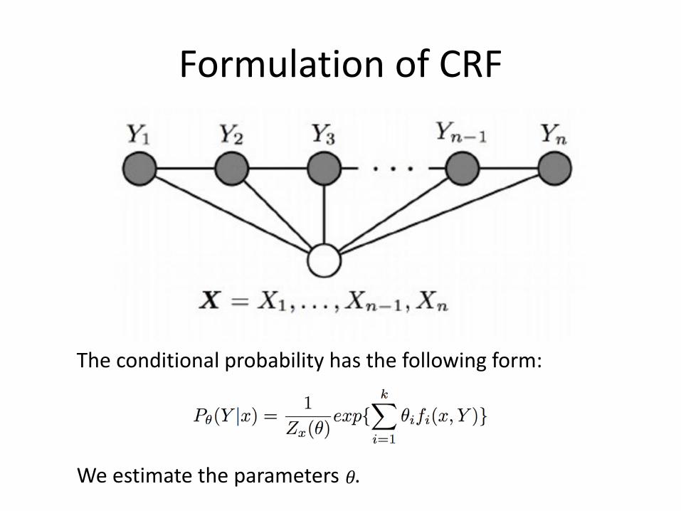
Formulation of CRF
The conditional probability has the following form:
We estimate the parameters .𝜃𝜃
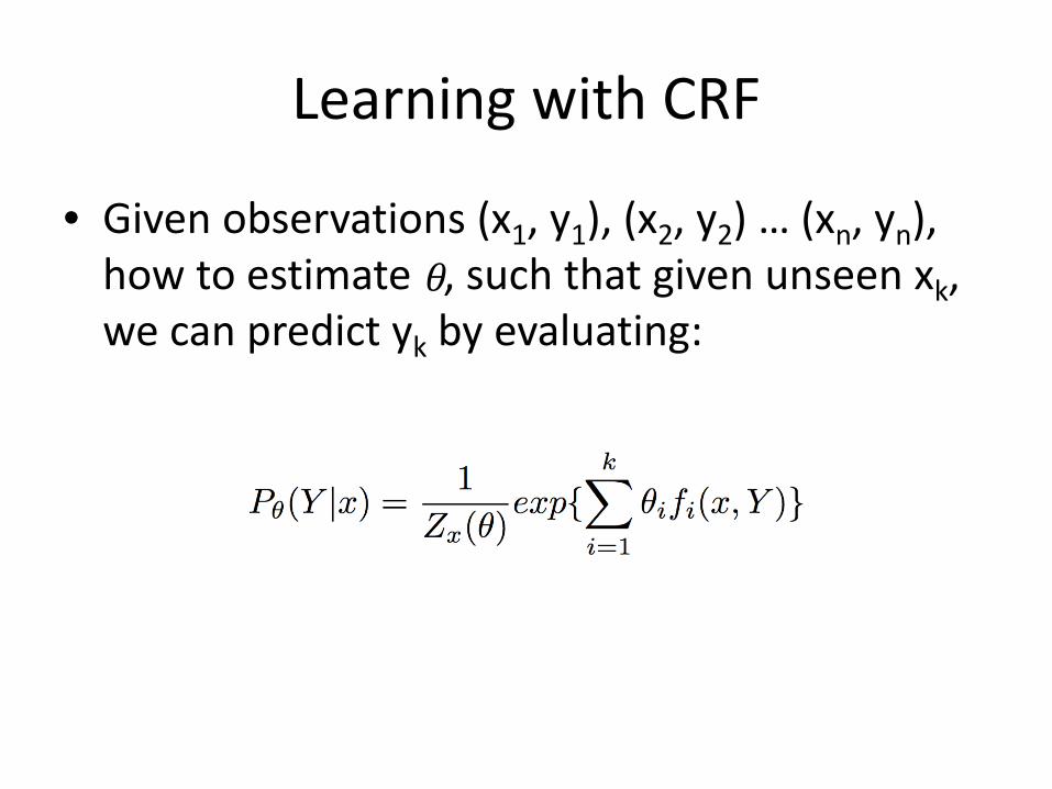
Learning with CRF
• Given observations (x1, y1), (x2, y2) … (xn, yn),how to estimate , such that given unseen xk,we can predict yk by evaluating:
𝜃𝜃

MLE and MAP of CRF
• MLE
The above formulation of ML/MAP learning can be kernelized using the Representer Theorem.
• MAP
Gaussian:
Laplacian:

Kernel CRF
• Representer Theorem for CRF
Objective Function:
Mercer Kernel:
The solution has the following form:
Study on Structured Sparsity
Yang Yang
May 4, 2017
1

Block-coordinate Descent Algorithms
1 1)(L ‖ ‖
group 2
1
( )k
m
k G
k
‖ ‖
overlap inf ,) .( , . p
G G G G G Gv
vv s t v
‖ ‖
0
,1
( | | ,)k k
m
k kk
N N
‖ ‖
Proximal methods Network flow algorithms
1
1ˆ arg min ) ),,( (N
i ii
xN
L y
y X
Sparse variable selection has wide applications-- signal processing, computer vision, computational biology…
Standard sparsity: consider individual variables equallyStructured sparsity: utilize spatial structures of variables
Standard Lasso
Group Lasso with disjoint groups
Overlapping group lasso
Hierarchical sparsity
Optimization methods
Bach et al. 2012
1{ , , }MG G
2

Huang et al.(2011) : under strongly group-sparse assumption, the group Lasso has superior performance over the standard Lasso
2
2ˆ ln( /(( g ) / n)O k m ‖ ‖
2
2 (( g )) /ˆ ln( n)/k m g ‖ ‖
2 2
2 2( , )
(2 )sup [ ln ( ) / ( 2) ln 4]
24 (2 )( )y
H g k
gg m g g g
n g
‖ ‖
1 2 202 (1 0.25 )
( )
cc A k gB
s n
‖ ‖Theorem 2:
Theorem 3:
1
2
2 0ˆ (( ln( / )) / )L O p n ‖ ‖ ‖ ‖
, |supp( ) , || |S SGG k S g (g,k) strongly group-sparse:
Nardi (2011): group Lasso is asymptotically optimal; offers the same asymptotic guarantees as the least squares estimator• model selection consistency
21/OLS
G h
‖ ‖ , for someLet 0 , such that ( 1)/2n , if 0n
0{ } 1, as n ˆ{ : 0}hh
( ) dn Z 0 0 0
2 1~ (0, ), and 0cZ M Z
• estimation consistency
Theorem 1:
1
2
2ˆ ( ln( / ) / )L k p k n ‖ ‖
Upper bound:
Lower bound:
Standard Lasso
Group Lasso with disjoint groups
3

Obozinski et al. (2011): support recovery - the support of መ𝛽matches the support of ҧ𝛽 with high probability
1 1ˆ( ) ( ) Theorem 4:
Theorem 5:
with probability approaching to 1
1 1 1ˆ( ) ( ) ( ) with high probability
Percival et al.(2011): overlapping group Lasso shares many of the same theoretical guarantees as the group Lasso, if the sets of groups are not too complex.
2
2
1 64ˆ( ) max | | max | | log( )G GX G A G Mn n
‖ ‖
1/2
2,1,
32ˆ max | | max | | log( )G GG A G Mn
‖ ‖
Theorem 6:
Zhao et al.(2009): Composite Absolute Penalties (CAP) family; particular overlapping patterns of groups are designed; with-in group and group-wise sparsity imposed
Overlapping Group Lasso
Hierarchical sparsity
4

Thank you!
5

Word embeddings, how do they work?
Ezra WinstonStatML, spring 2017
CMU
May 4, 2017

Word Embeddings
I Given vocabulary w1,w2, . . . ,wn, word embeddings are vectorsv1, v2, . . . , vn ∈ Rd .
I Goal is to capture the semantics of words in a low dimensionalspace. Typically d ≈ 300 while n ≈ 105.
I Shown to improve performance when used as features in NLPtasks, compared to, say, one-hot encoding of words whered = n.

Example: word2vec (Mikolov et al. 2013)
I Embeddings vi learned on a large textcorpus by modeling probability of wordwi appearing given context word wj .
I Approximates softmax objective
P(wj |wi ) =exp(v>j hi )∑nk=1 exp(v>k hi )
where hi are context embeddings andvi are output embeddings.

Theoretical Questions
I Under what assumptions are popular embedding methodsconsistent?
I Why do low dimensional vectors capture the semantics well?I Many more: relations ≈ directions, syntax words, polysemy. . .

Theoretical Questions
I Under what assumptions are popular embedding methodsconsistent?
I Why do low dimensional vectors capture the semantics well?
I Many more: relations ≈ directions, syntax words, polysemy. . .

Theoretical Questions
I Under what assumptions are popular embedding methodsconsistent?
I Why do low dimensional vectors capture the semantics well?I Many more: relations ≈ directions, syntax words, polysemy. . .

Explanation 1: Arora et al. 2016
Setup:I Language generation is a random walk of a unit-length
discourse vector ct ∈ Rd
I Embedding vectors are approximately uniformly distributed inspace.
I ct is a slow random walk: stationary distribution has‖ct − ct−1‖2 < ε2/
√d .
I The probability of word w being emitted at time t isp(w |ct) ∝ exp(〈ct , vw 〉).
Theorem
log p(wi ,wj) =‖vi + vj‖
2d− 2 logZ ± ε
where Z is a constant that is close to the partition function andε = O( 1√
n) + O( 1
d ) + O(ε2).
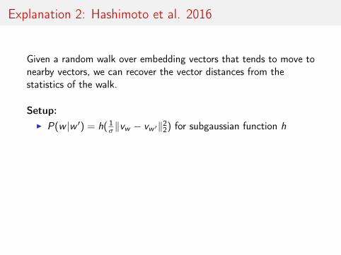
Explanation 2: Hashimoto et al. 2016
Given a random walk over embedding vectors that tends to move tonearby vectors, we can recover the vector distances from thestatistics of the walk.
Setup:I P(w |w ′) = h( 1
σ‖vw − vw ′‖22) for subgaussian function h
TheoremLet Cm,n
ij (tn) be the number of times word wj occurs tn words afterwi . There exists ai and bj such that simultaneously over all i , j :
limn→∞
− log(Cm,nij (tn))− am,ni − bm,nj → ‖xi − xj‖22

Graph-Based Semi-Supervised Classification and the Graph Construction
Xuan Wu
Institute for Software Research
Carnegie Mellon University

Motivation
• Labeled data is very few and expensive to obtain
• Unlabeled data is widely available, but barely utilized
• Graph-based SSL methods provide uniform representation for heterogeneous data, and are parallelizable, scalable to large data
• In many tasks, we need to first construct the similarity graph
• Different graphs can lead to different classification accuracies

Gaussian Random Fields Method
• GRF defined as follows:
, where
To maximize subject to for all labeled data,
the solution is harmonic, satisfying
on unlabeled data set, and on labeled data.
And is given by
( )
( )E fe
P fZ
2
,
1( ) ( ( ) ( ))
2ij
i j
E f w f i f j
( )P f ( ) ( )l if i f i y
0f lf f
uf1( )uu ul lI P P f

Global and Local Consistency Method
Closed Form Solution: * 1( )F I S Y
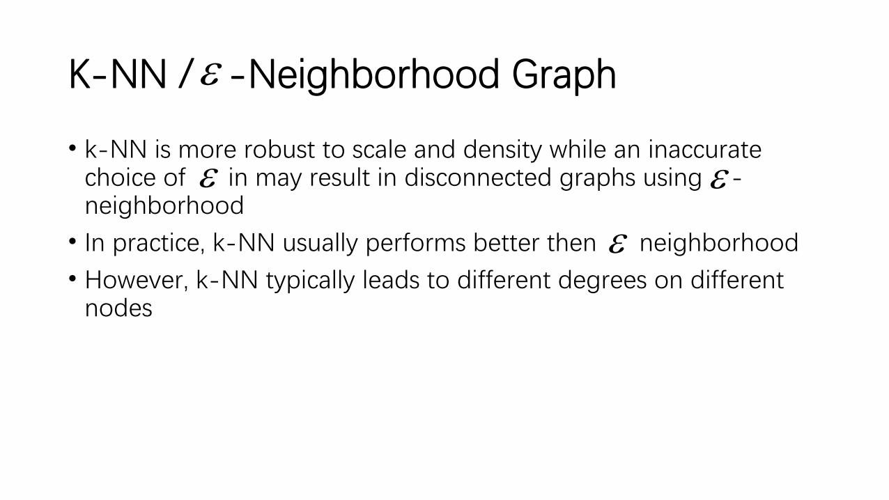
K-NN / -Neighborhood Graph
• k-NN is more robust to scale and density while an inaccurate choice of in may result in disconnected graphs using -neighborhood
• In practice, k-NN usually performs better then neighborhood
• However, k-NN typically leads to different degrees on different nodes

Graph Construction with B-Matching
• The first step is graph sparsification, in which we select a subset of edges to satisfy
• The second step is Edge Re-Weighting. Available methods include Binary, Gaussian Kernel, and Locally Linear Reconstruction (LLR)

Graph Construction with Spectral Transform
• Consider the following form of kernel
, where are the eigenvectors of the graph La
Laplacian .
• We want to choose s.t the outer product of smaller eigenvalue has higher weight.
• To determine s, zhu et al. proposed to maximize the empirical kernel alignment
is
iL
i

Thank You!


Reinforcement Learning
Markov Decision Processes with finite state & action space, finite timehorizon M = (S,A,R,P,H, ρ):
S: state space, A: action space.
R: reward function. H: time horizon in an episode.
P: transition probability. ρ: initial state distribution.
An RL algorithm π sequentially maps the sample history to a policy µk ,k = 1, ...,T/H, evaluated by its regret (stronger than risk):
Regret(T , π,M) =
T/H∑k=1
VM(µ∗M)− VM(µk) .
Bayes regret: assume M drawn from prior φ,
BayesRegret(T , π, φ) = E [Regret(T , π,M)|M ∼ φ] .
2 / 3

Algorithms (Model Based)
Confidence set based algorithm:Before each episode k , construct a confidence set Mk for M, act usingthe policy that is the most optimistic according to Mk , update theconfidence set.Best known result: maxM Regret(T , π,M) = O(HS
√AT ) with high
prob.A general proof technique:
VM(µ∗M)− VM(µk) = VM(µ∗
M)− VMk(µk) + VMk
(µk)− VM(µk)
≤ VMk(µk)− VM(µk) . (1)
Posterior sampling algorithm:Before each episode k , sample an MDP Mk from the posteriordistribution Hk for M, act using the optimal policy for Mk , update theposterior.Best known result: BayesRegret(T , π, φ) = O(HS
√AT ).
A general reduction: for any high prob. regret bound for a confidenceset based algorithm derived using (1), the same Bayes regret holdsfor the posterior sampling algorithm.
3 / 3

Modeling Correlated Times Series Data
Chenghui Zhou

Predictive Linear Gaussian Model
𝑦𝑦𝑡𝑡𝑦𝑦𝑡𝑡+1
…𝑦𝑦𝑡𝑡+𝑑𝑑−1𝑦𝑦𝑡𝑡+𝑑𝑑
= 𝐺𝐺
𝑦𝑦𝑡𝑡−1𝑦𝑦𝑡𝑡…
𝑦𝑦𝑡𝑡+𝑑𝑑−2𝑦𝑦𝑡𝑡+𝑑𝑑−1
+
00…0
𝜖𝜖𝑡𝑡+𝑑𝑑
(PLG)

Predictive Linear Gaussian Model
𝑦𝑦𝑡𝑡𝑦𝑦𝑡𝑡+1
…𝑦𝑦𝑡𝑡+𝑑𝑑−1𝑦𝑦𝑡𝑡+𝑑𝑑
= 𝐺𝐺
𝑦𝑦𝑡𝑡−1𝑦𝑦𝑡𝑡…
𝑦𝑦𝑡𝑡+𝑑𝑑−2𝑦𝑦𝑡𝑡+𝑑𝑑−1
+
00…0
𝜖𝜖𝑡𝑡+𝑑𝑑
Observation at time t
𝑌𝑌𝑡𝑡

Predictive Linear Gaussian Model
𝑦𝑦𝑡𝑡𝑦𝑦𝑡𝑡+1
…𝑦𝑦𝑡𝑡+𝑑𝑑−1𝑦𝑦𝑡𝑡+𝑑𝑑
= 𝐺𝐺
𝑦𝑦𝑡𝑡−1𝑦𝑦𝑡𝑡…
𝑦𝑦𝑡𝑡+𝑑𝑑−2𝑦𝑦𝑡𝑡+𝑑𝑑−1
+
00…0
𝜖𝜖𝑡𝑡+𝑑𝑑Update matrix

Predictive Linear Gaussian Model
𝑦𝑦𝑡𝑡𝑦𝑦𝑡𝑡+1
…𝑦𝑦𝑡𝑡+𝑑𝑑−1𝑦𝑦𝑡𝑡+𝑑𝑑
= 𝐺𝐺
𝑦𝑦𝑡𝑡−1𝑦𝑦𝑡𝑡…
𝑦𝑦𝑡𝑡+𝑑𝑑−2𝑦𝑦𝑡𝑡+𝑑𝑑−1
+
00…0
𝜖𝜖𝑡𝑡+𝑑𝑑Update matrix
noise

Predictive Linear Gaussian Model
𝑦𝑦𝑡𝑡𝑦𝑦𝑡𝑡+1
…𝑦𝑦𝑡𝑡+𝑑𝑑−1𝑦𝑦𝑡𝑡+𝑑𝑑
= 𝐺𝐺
𝑦𝑦𝑡𝑡−1𝑦𝑦𝑡𝑡…
𝑦𝑦𝑡𝑡+𝑑𝑑−2𝑦𝑦𝑡𝑡+𝑑𝑑−1
+
00…0
𝜖𝜖𝑡𝑡+𝑑𝑑New observation Update
matrixnoise
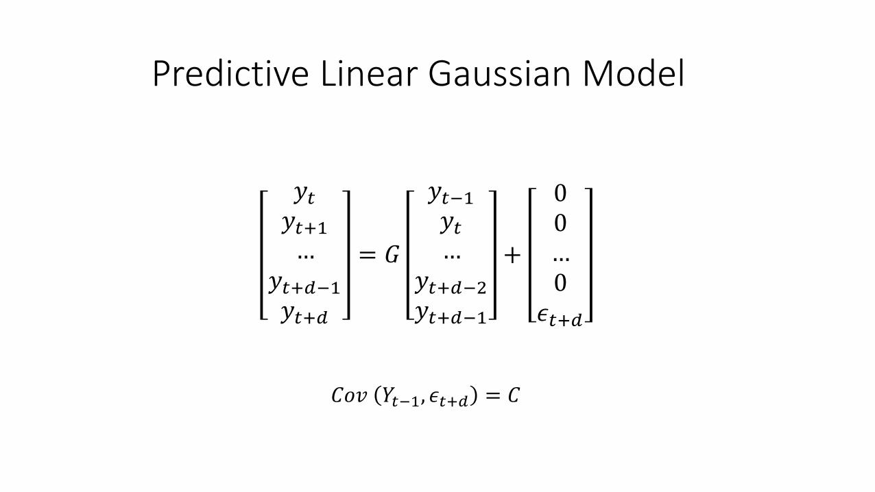
Predictive Linear Gaussian Model
𝑦𝑦𝑡𝑡𝑦𝑦𝑡𝑡+1
…𝑦𝑦𝑡𝑡+𝑑𝑑−1𝑦𝑦𝑡𝑡+𝑑𝑑
= 𝐺𝐺
𝑦𝑦𝑡𝑡−1𝑦𝑦𝑡𝑡…
𝑦𝑦𝑡𝑡+𝑑𝑑−2𝑦𝑦𝑡𝑡+𝑑𝑑−1
+
00…0
𝜖𝜖𝑡𝑡+𝑑𝑑
𝐶𝐶𝐶𝐶𝐶𝐶 𝑌𝑌𝑡𝑡−1, 𝜖𝜖𝑡𝑡+𝑑𝑑 = 𝐶𝐶

Relation with Other Models
Linear Dynamical System (LDS)𝑥𝑥𝑡𝑡 = 𝑇𝑇 𝑥𝑥𝑡𝑡−1 + 𝜎𝜎𝑡𝑡𝑦𝑦𝑡𝑡 = 𝑂𝑂 𝑥𝑥𝑡𝑡 + 𝛿𝛿𝑡𝑡
𝜎𝜎𝑡𝑡 ~ 𝑁𝑁 0, Σ𝛿𝛿𝑡𝑡 ~ 𝑁𝑁(0,Δ)𝑥𝑥0~ 𝑁𝑁(𝜇𝜇0,𝑃𝑃0)
Transition matrix
Observation matrix

Relation with Other Models
Linear Dynamical System (LDS)𝑥𝑥𝑡𝑡 = 𝑇𝑇 𝑥𝑥𝑡𝑡−1 + 𝜎𝜎𝑡𝑡𝑦𝑦𝑡𝑡 = 𝑂𝑂 𝑥𝑥𝑡𝑡 + 𝛿𝛿𝑡𝑡
𝜎𝜎𝑡𝑡 ~ 𝑁𝑁 0, Σ𝛿𝛿𝑡𝑡 ~ 𝑁𝑁(0,Δ)𝑥𝑥0~ 𝑁𝑁 𝜇𝜇0,𝑃𝑃0
• Parameter G is a function of transition matrix and observation matrix• Covariance C is a function of G, Δ, Σ and 𝑃𝑃0• Predictive Linear Gaussian Model is equivalent to LDS

Relation with Other Models
Autoregressive and Moving Average Model (ARMA)
𝑦𝑦𝑡𝑡 = �𝑖𝑖=1
𝑑𝑑
Φ𝑖𝑖 𝑦𝑦𝑡𝑡−𝑖𝑖 + 𝑎𝑎𝑡𝑡 + �𝑖𝑖=1
𝑝𝑝
𝜃𝜃𝑖𝑖 𝑎𝑎𝑡𝑡−𝑖𝑖
White noise
weights

Relation with Other Models
Autoregressive and Moving Average Model (ARMA)
𝑦𝑦𝑡𝑡 = �𝑖𝑖=1
𝑑𝑑
Φ𝑖𝑖 𝑦𝑦𝑡𝑡−𝑖𝑖 + 𝑎𝑎𝑡𝑡 + �𝑖𝑖=1
𝑝𝑝
𝜃𝜃𝑖𝑖 𝑎𝑎𝑡𝑡−𝑖𝑖
• Φ𝑖𝑖’s can be seen as each entry in the update matrix G• LDS subsumes ARMA model• ARMA model can be represented by Predictive Linear Gaussian Model

Stochastic gradient method and its application
Yifan Sun
Deparment of Mathematical SciencesCarnegie Mellon University
May 1, 2017
Yifan Sun (Department of Mathematical Sciences) Short title May 1, 2017 1 / 17

Overview
1 Vanilla SGD
2 SVRG technique
3 Acceleration of SGD
4 SGD on PCA
Yifan Sun (Department of Mathematical Sciences) Short title May 1, 2017 2 / 17

Vanilla SGD
In machine learning we often encounter the following problem:
minimizex∈Rd
{F (x) = f (x) + φ(x) =
1n
n∑i=1
fi (x) + φ(x)
}where f(x) is usually the loss function and φ(x) is the regularization term. Alot of regularized empirical risk minimization problem could be written aboveform, for example Ridge regression, Lasso, SVM.
Yifan Sun (Department of Mathematical Sciences) Short title May 1, 2017 3 / 17

Vanilla SGD
For simplicity we assume there is no regularization term, and the usualgradient descent method is:
x (t) ← x (t−1) − ηtn
n∑i=1
∇fi (x (t−1))
Yifan Sun (Department of Mathematical Sciences) Short title May 1, 2017 4 / 17

Vanilla SGD
However, when n is large, the calculation of n derivatives in one iteration isvery expensive. The vanilla stochastic gradient descent method choose oneparticular index uniformly from i ∈ {1, ...n} and calculates:
x (t) ← x (t−1) − ηt∇fi (x (t−1))
More generally, the SGD updates has the form:
x (t) ← x (t−1) − ηtg(x (t−1)) (1)
E[g(x (t−1))] = ∇f (x (t−1)) (2)
Yifan Sun (Department of Mathematical Sciences) Short title May 1, 2017 5 / 17
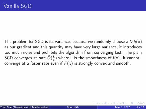
Vanilla SGD
The problem for SGD is its variance, because we randomly choose a ∇fi (x)as our gradient and this quantity may have very large variance, it introducestoo much noise and prohibits the algorithm from converging fast. The plainSGD converges at rate O(Lε ) where L is the smoothness of f(x). It cannotconverge at a faster rate even if F (x) is strongly convex and smooth.
Yifan Sun (Department of Mathematical Sciences) Short title May 1, 2017 6 / 17

SVRG
Johnson and Zhang[2013] proposed a variance reduction method.The keyidea is to take a snapshot vector x = xk as well as its full gradientµ = ∇f (x) once in every m iteration. The key observation is if we randomlypick one i ∈ {1...n}, we have E[∇fi (x)− µ] = 0. Then we can add thisterm to our gradient update and get the update rule:
x (t) ← x (t−1) − ηt(∇fi (x (t−1))−∇fi (x) + µ)
Yifan Sun (Department of Mathematical Sciences) Short title May 1, 2017 7 / 17

SVRG
The magic here is that as x (k) → x∗, we have ∇fi (x (k))→ ∇fi (x) andµ = ∇f (x)→ 0 hence the variance of the update gradient∇k = ∇fi (x (k))−∇fi (x) + µ goes to 0. The iteration complexity isO((n + κ) log 1
ε ) where κ = Lµ is the condition number.
Yifan Sun (Department of Mathematical Sciences) Short title May 1, 2017 8 / 17

Acceleration of SGD
Nesterov’s method could be used for deterministic gradient descentacceleration, the idea is to do update by:
y = x (k−1) +k − 2k + 1
(x (k−1) − x (k−2))
x (k) = y − tk∇f (y)
where the x (k−1) − x (k−2) term is a momentum term that makes us "goalong the descending direction for more distance". In gradient descent thismomentum accelerates the convergence, however in SGD since our updatesis random, the update direction from last steps could deviate far from thefull gradient and hence accumulates the incorrect momentum will lead todivergence of the algorithm.
Yifan Sun (Department of Mathematical Sciences) Short title May 1, 2017 9 / 17

Acceleration of SGD
Allen-Zhu[2017] proposed the state of art acceleration method for SGDcalled ’Katyusha’ which converges at rate O((n +
√nκ) log 1
ε ) for L-smoothand α-strongly convex function. The update rule is:
x (k+1) ← τ1zk + τ2x + (1− τ1 − τ2)yk (3)
∇k+1 ← ∇f (x) +∇fi (xk+1)−∇fi (x) (4)
y (k+1) ← x (k+1) − 13L∇k+1 (5)
z(k+1) ← z(k) − α∇k+1 (6)
Yifan Sun (Department of Mathematical Sciences) Short title May 1, 2017 10 / 17

Acceleration of SGD
The key idea is to keep a snapshot of x , and by choosing τ2 = 0.5, in (3)the updates guarantees that the update of x (k+1) will not deviate too muchfrom the snapshot. This can be seen as a ’negative momentum’ whichreduces the risks of going in the incorrect momentum direction too much.z(k) and y (k) in (3) give the ’momentum’ term. (5) and (6) comes out ofthe idea of linearly coupling gradient descent and mirror descent algorithm in[Allen-Zhu and Orecchia 2014], which guarantees the algorithm to descendfast enough no matter ||∇k+1|| is large or small.
Yifan Sun (Department of Mathematical Sciences) Short title May 1, 2017 11 / 17

SGD on PCA
Shamir considers the problem of finding the largest eigenvector:
minw∈Rd :||w ||2=1
−wT (1n
n∑i=1
xixTi )w
Yifan Sun (Department of Mathematical Sciences) Short title May 1, 2017 12 / 17

SGD on PCA
The algorithm from [Shamir2015] keeps a snapshot w andu := 1
n
∑ni=1 xi (x
Ti w) for m periods, and within this m periods, it picks
it ∈ {1, ...n} uniformly, then the update rule is:
w ′t ← wt−1 + ηt(xitxTit wt−1 − xitx
Tit w + u) (7)
wt ←w ′t||w ′t ||
(8)
Yifan Sun (Department of Mathematical Sciences) Short title May 1, 2017 13 / 17
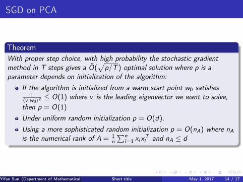
SGD on PCA
TheoremWith proper step choice, with high probability the stochastic gradientmethod in T steps gives a O(
√p/T ) optimal solution where p is a
parameter depends on initialization of the algorithm:If the algorithm is initialized from a warm start point w0 satisfies
1〈v ,w0〉2 ≤ O(1) where v is the leading eigenvector we want to solve,then p = O(1)Under uniform random initialization p = O(d).Using a more sophisticated random initialization p = O(nA) where nAis the numerical rank of A = 1
n
∑ni=1 xix
Ti and nA ≤ d
Yifan Sun (Department of Mathematical Sciences) Short title May 1, 2017 14 / 17

SGD on PCA
The proof of the theorem is very elaborate. It uses Azuma-Hoeffdinginequality on martingales, conditional expectation technique and matrixalgebra.
Yifan Sun (Department of Mathematical Sciences) Short title May 1, 2017 15 / 17

References
Allen-Zhu, Z. and Orrechia, L.Linear coupling, an ultimate unification of gradient and mirror descent.Informs Annual Meeting, 2014.
Allen-Zhu (2017)Katyusha: The First Direct Acceleration of Stochastic Gradient MethodsIn Symposium on Theory of Computing(STOC), 2017.
Johnson, R. and Zhang, T. (2013)Accelerating stochastic gradient descent using predictive variance reduction.In NIPS, 2013In Symposium on Theory of Computing(STOC), 2017.
Shamir, O. (2015)A Stochastic PCA and SVD Algorithm with an Exponential Convergence RateIn ICML, 2015
Shamir, O. (2017)Fast stochastic algorithms for SVD and PCA: convergence properties and convexity.In ICML, 2017, doi:https://arxiv.org/pdf/1507.08788.pdf
Yifan Sun (Department of Mathematical Sciences) Short title May 1, 2017 16 / 17

Thanks!
Yifan Sun (Department of Mathematical Sciences) Short title May 1, 2017 17 / 17

A Survey of Theories on Generative Adversarial
NetworksChris Ying, Yijie Wang
May 4, 2017

GAN Minimax Value Function
g= generator parameters G = generator function
d= discriminator parameters D = discriminator function
pdata= true distribution pz= noise distribution
discriminator output on generated data
Goodfellow, Ian, et al. "Generative adversarial nets." Advances in neural information processing systems. 2014.
discriminator output on true data

Theoretical Results
Optimal D:
At optimality:
With sufficient model capacity, optimality is reached
pdata
G
D
Goodfellow, Ian, et al. "Generative adversarial nets." Advances in neural information processing systems. 2014.

Loss-Sensitive Generative Adversarial Networks on Lipschitz Densities● Finite model capacity● Lipschitz property assumption on the underlying distribution, on the model
parameters and on the model inputs● Adaptive margin:
● Objective:
● Theoretical properties:○ Convergence of generated distribution based on Nash Equilibrium○ Probabilistically approximate generalization bound given for both the
generator and the discriminator
Qi, Guo-Jun. "Loss-sensitive generative adversarial networks on lipschitz densities." arXiv preprint arXiv:1701.06264 (2017).

Wasserstein GAN
● Uses Earth-Mover distance (a.k.a. Wasserstein-1 distance) instead of Jensen-Shannon divergence:
● New value function (assume generator fixed, f parametric family K-Lipschitz):
● Desirable properties of Earth-Mover distance:○ Continuous and differentiable almost everywhere○ Guarantee of convergence similar to Jensen-Shannon divergence
Arjovsky, Martin, Soumith Chintala, and Léon Bottou. "Wasserstein gan." arXiv preprint arXiv:1701.07875 (2017).

Predictive State RepresentationAn alternate approach to learn dynamical systems
Boyue LiMay 1, 2017
Language Technologies Institute

Introduction

1.1. Dynamical system
A dynamical system is asystem whose• output is decided by itsstate and noise
• state evolves with timeover a state space
• state evolves accordingto a fixed rule
HMM and RNN are alldynamical systems[1, 2, 5].
More specifically,
st+1 = f(st) (1)ot = g(st) + ϵt (2)
Figure 1: A dynamical system[3].
1
1.2. Spectral algorithm
Spectral algorithms factorize matrices of observable momentsto learn a consistent model.
These algorithms are usually
• fast (comparing to E-M and RNN!)• simple• consistent• globally optimum
2

Predictive state representation

2.1. Formulation
Figure 2: Predictive state representation[3].
where ψt = ψ(ot:t+k−1) is future feature, ξt = ξ(ot:t+k) isextended future feature and ht = h(o1:t−1) is history feature. 3

2.1. Formulation
• PSR is not popular, but it has good theoretical properties.• Model hierarchy: HMM < PSR < RNN.• PSR can be extend to non-linear discrete spaces andcontinuous space using a Hilbert Space Embeddingtechnique.
4

2.2. Spectral learning algorithm
Define
• qt = qt|t−1 = E[ψt | o1:t−1] determins P(ot:t+k−1 | o1:t−1)• pt = pt|t−1 = E[ξt | o1:t−1] determins P(ot:t+k | o1:t−1)
For a linear system, pt = Wqt. we have
E[pt | ht] = E[Wqt | ht] (3)
E[E[ξt | o1:t−1] | ht
]= WE
[E[ψt | o1:t−1] | ht
](4)
E[ξt | ht] = WE[ψt | ht] (5)
We can estimate E[ξt | ht], E[ψt | ht] from training data, thenuse ridge regression to calculate W. The initial state q1 = E[ψ1].To update states, we use qt+1 = ffilter(pt,ot) or qt+1 = fpredict(pt).
5

2.3.1. Refining model: Gradient Descent
If qt+1 = ffilter(qt,ot) =Botqt
qT∞Botqt,
where q∞ is a normalizationvector.The negative log likelihoodfunction is
L(B1, ...,BM)=− log(P(O))=− log(qT∞BoTBoT−1 ...B1q1)
Then, we can use gradientdescent to refine thismodel[4].
Figure 3: Character-levellanguage model performance onWikipedia data[4]. RNN couldreach 1.5 - 1.6 bpc[6]. 6

2.3.2. Refining model: RNN
PSR and RNN have very similarrecursive structures. What ifwe use a RNN to refine a PSR?We can just applyspectral-learned weights to aRNN and use normal trainingalgorithms to refine it.
Figure 4: Character-level languagemodel performance onPennTreebank.
7

Thanks!
7

References I
Z. Ghahramani and G. E. Hinton.Parameter Estimation for Linear Dynamical Systems.Technical Report, 6(CRG-TR-96-2):1–6, 1996.
Z. Ghahramani and S. T. Roweis.Learning Nonlinear Dynamical Systems using an EMAlgorithm.Advances in Neural Information Processing Systems 11,(1):599–605, 1999.A. Hefny, C. Downey, and G. Gordon.Supervised Learning for Dynamical System Learning.pages 1–32, 2015.

References II
N. Jiang, A. Kulesza, and S. Singh.Improving Predictive State Representations via GradientDescent.Proceedings of the 30th Conference on ArtificialIntelligence (AAAI 2016), pages 1709–1715, 2016.
J. Langford, R. Salakhutdinov, and T. Zhang.Learning Nonlinear Dynamic Models.Proceedings of the 26th Annual International Conferenceon Machine Learning ICML 09, cs.AI(1):1–8, 2009.
J. Martens.Generating Text with Recurrent Neural Networks.Neural Networks, 131(1):1017–1024, 2011.

Overview of Q-Learning Convergence
Vivek Nangia
Carnegie Mellon University
May 4, 2017
Vivek Nangia (CMU) Short title May 4, 2017 1 / 13

Introduction to Reinforcement Learning
Agent moving around some discrete, finite world
Choose action from finite collection of actions at every step
At time n, agent at state xn ∈ X choses action an ∈ A
The agent receives probabilistic reward rn. Mean value Rxn(an) isdependent only on state and action.
Agent moves to next state yn with dynamics
Pr(yn = y |sn, an) = Pxny [an]
Goal: Determine optimal policy that maximizes total expecteddiscount reward
Vivek Nangia (CMU) Short title May 4, 2017 2 / 13

State Value Functions
For a given policy π, the value of state x is defined as:
V π(x) = Rx(π(x)) + γ∑y
Pxy [π(x)]V π(y)
The agent expects to receive Rx(π(x)) immediately and the moves toa state that is ’worth’ V π(y) with probability Pxy [π(x)]
Vivek Nangia (CMU) Short title May 4, 2017 3 / 13

Optimal State Value
Dynamic programming theory states there exists at least one optimalpolicy π∗ such that
V ∗(x) = V π∗(x) = max
a
(Rx(a) + γ
∑y
Pxy [a]V π∗(y)
)
This is a well defined recursive definition with the ability determineV ∗ and π∗ assuming Rx(a) and Pxy [a] are known.
Vivek Nangia (CMU) Short title May 4, 2017 4 / 13

Q Values
For a policy π, define Q values (action-values) as:
Qπ(a, x) = Rx(a) + γ∑y
Pxy [π(x)]V π(y)
Q value is the expected discounted reward for executing action a atstate x and then following policy π
Vivek Nangia (CMU) Short title May 4, 2017 5 / 13

Q - Learning
Seeks to learn Q values, state for optimal policy π∗
V ∗(x) = maxa Q∗(x , a)
This leads to the policy π∗(x) = a∗
Vivek Nangia (CMU) Short title May 4, 2017 6 / 13

Episodes
Stepping through the environment consists of distance episodes
The nth episodes is defined as the tuple (xn, an, yn, rn, αn)
Current state xnCurrent action anSubsequent state ynReward rnLearning factor αn where
Qn(x , a) = (1− αn)Qn−1(x , a) + αn[rn + γVn−1(yn)]
Vivek Nangia (CMU) Short title May 4, 2017 7 / 13

Conditions on Convergence
Qn(x , a) is represented as a lookup table
Sequence of episodes has infinite length
Episodes need not be continuous
Vivek Nangia (CMU) Short title May 4, 2017 8 / 13
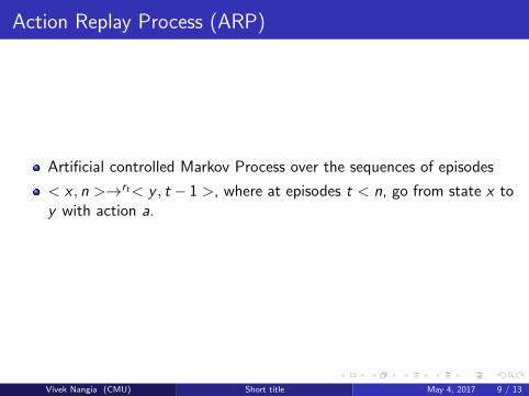
Action Replay Process (ARP)
Artificial controlled Markov Process over the sequences of episodes
< x , n >→rt< y , t − 1 >, where at episodes t < n, go from state x toy with action a.
Vivek Nangia (CMU) Short title May 4, 2017 9 / 13

Lemma A
Qn(x , a) are the optimal action values for the ARP states < x , n > andactions
Vivek Nangia (CMU) Short title May 4, 2017 10 / 13

Lemma B
Given a finite Markov process, from any starting state x , the differentbetween the value of that state under the finite sequences of s actionsand its value under the same sequences followed by any other actiontends to 0 as n⇒∞Given l , there exists a higher level h such that the probability can bemade arbitrarily small of moving below l after taking s actions in theARP
With probability 1, the probabilities of the ARP and reward functionof the ARP tend to those values in the real process as the level nincreases to infinity
As the dynamics and expected reward functions of the ARP and realprocess converge, the Q values of all states converge
Vivek Nangia (CMU) Short title May 4, 2017 11 / 13

Proof
The ARP tends toward the real process, and so its optimal Q values do aswell. But Qn(a, x) are the optimal Q values for the nth level of the ARP,and therefore tend to Q∗(x , a)
Vivek Nangia (CMU) Short title May 4, 2017 12 / 13

The End
Vivek Nangia (CMU) Short title May 4, 2017 13 / 13

Monte Carlo Methods for Sampling
Hengyuan Hu, Quanbin Ma

Motivation
Sampling is pervasive in statistics and machine learning.- Draw samples from arbitrary distribution.- Use samples to estimate intractable terms.- Extremely hard especially in high dimension.
Use Monte Carlo methods to trade accuracy for efficiency.

Markov Chain Monte Carlo for sampling
Metropolis Hastings Algorithm- Given a state:- Proposal: go to any stochastic
perturbation of the state. - A common choice is following a
Gaussian: Random Walk- Correction: rejects any proposals
that stray too far away from the target distribution.
- Consecutive steps are highly correlated: inefficient exploration

- Model not only the state, but also velocity.
- Formulated under framework of Hamiltonian dynamics to ensure basic properties of MCMC are satisfied.
- Instead of walking, we are now kicking a ball around.
Hamiltonian Monte Carlo

Samples generated for an 100-dimensional Gaussian. (Neal 2011)
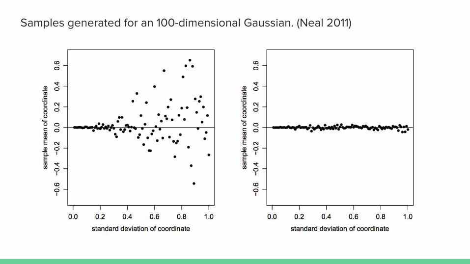
Samples generated for an 100-dimensional Gaussian. (Neal 2011)

Samples generated for an 100-dimensional Gaussian. (Neal 2011)

Probabilistic Inference in Graphical Modelsvia Markov chain Monte Carlo Method
Yuan Liu (刘源)

MotivationWhat is inference?◦ Let 𝐹, 𝐸 be two disjoint subsets of the random variables 𝑉. Denote 𝑅 = 𝑉 − 𝐸 − 𝐹. Theprobabilistic inference is to calculate: 𝑝 𝑥𝐹 𝑥𝐸 =
∑ 𝑝(𝑥𝐸,𝑥𝐹,𝑥𝑅)�𝑥𝑅
∑ 𝑝(𝑥𝐸,𝑥𝐹,𝑥𝑅)�𝑥𝑅,𝑥𝐹
◦ The calculation of 𝐸𝑥∼𝑝[𝑓(𝑥)]
Why it is important?◦ We always need to calculate the marginal distribution.
◦ Write the Markov Random Field in log-linear form: 𝑝 𝑥𝑉 = 1𝑍 exp(∏ 𝑤𝑐𝐹𝑐(𝑥𝑐)�
𝑐∈𝐶 ). Thederivation has the following form: 𝜕
𝜕𝑤𝑐𝑙 𝑤: 𝐷 = ∑ 𝐹𝑐(𝑥𝑐)�
𝑥∈𝐷 − 𝐸𝑥∼𝑝[𝐹𝑐(𝑥𝑐)]

The Metropolis-Hastings AlgorithmThis algorithm maintains a record of the current state 𝑥(𝑡), and the proposaldistribution 𝑞𝑘(𝑥, 𝑥(𝑡)) depends on the current state.
𝐴𝑘 𝑥∗, 𝑥 𝑡 = min(1, 𝑝 𝑥∗ 𝑞𝑘(𝑥∗,𝑥(𝑡))
𝑝 𝑥 𝑡 𝑞𝑘(𝑥 𝑡 ,𝑥∗))
◦ Prove the convergence of this algorithm.◦ Burning–in the sampler.◦ Simulated Annealing.◦ Effective sample size.

Gibbs SamplingGibbs sampling is a special case of the Metropolis-Hasting algorithm.𝑞𝑘 𝑥, 𝑥I = 𝑝 𝑥𝑘I 𝑥JK .
◦ The main advantage of Gibbs sampling is the new state will always be accepted.◦ How to use it in the Markov Random Field. (Markov Blanket)◦ Blocking Gibbs Sampling◦ Convergence Diagnostics: The Gibbs Stopper.

Thank you

Asynchronous & ApproximateQ-learning
Emilio [email protected]
PhD StudentMachine Learning Department
Carnegie Mellon University

Reinforcement Learning
• Given an MDP 𝑆, 𝐴, 𝛾, 𝑃 𝑠′ 𝑠, 𝑎 , 𝑟 𝑠, 𝑎, 𝑠′
• Find a policy 𝜋 ∶ 𝑆 → 𝐴 that maximizes future reward.
• Q-function:• Expected future reward starting in state 𝑠, executing 𝑎, and following 𝜋
𝑄𝜋 𝑠, 𝑎 = 𝔼𝜋,𝑃 𝑡=0
∞
𝛾𝑡𝑟𝑡
• Satisfies the Bellman Equation:𝑄𝜋 𝑠, 𝑎 = 𝔼𝑎′~𝜋 ⋅ 𝑠 ,𝑠′~𝑃 ⋅ 𝑠, 𝑎 𝑟 𝑠, 𝑎, 𝑠′ + 𝛾𝑄𝜋 𝑠′, 𝑎′

Q learning
• Optimal Q-function satisfies Bellman Optimality Equation:
• We can extract optimal policy by choosing action with highest Q-value.
• Q-learning recovers optimal Q-value:
′

Asynchronous Q-learning Theorem
Meaning: If we use Q-learning update asynchronously, Q-learning still converges to optimal Q-value function with some minor assumptions on the MDP.
′
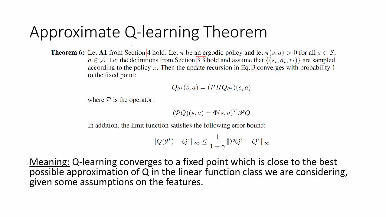
Approximate Q-learning Theorem
Meaning: Q-learning converges to a fixed point which is close to the best possible approximation of Q in the linear function class we are considering, given some assumptions on the features.

Thank you

Latent-Feature Model & Latent-Feature Lasso
Enxu Yan Xiaofei Shi

Problem Definition: Latent-Feature Model (LFM)
I LFM is a generalization of Mixture Model:
x = W T z + ω.
I z ∈ {0, 1}K : presence or absence of features {Wk,:}Kk=1.
I ω ∈ RD contains noise and bias due to model misspecify.
Goals:
I (i) Estimate W (if model is correct).
I (ii) Minimize r(W ) := E[minz∈{0,1}K ‖x −W T z‖2
].

Existing and New Results
Let r(W ) := E[minz∈{0,1}K ‖x −W T z‖2
]be the risk.
Table: Summary of Results (N=#samples, D=dim(x), K=#features).
Method Complexity Theoretical Guarantee Assumption
MCMC (NK2D) (Z (T ),W (T )) ∼ p(Z ,W |X ) as T →∞ Z ∼IBP(α), x ∼ N(WT z, σ2I )
Varitional (NK2D) n/a n/a
MF-Binary (NK)2K Exact Recovery Noiseless with cond. on Z∗
MAD-Bayes (NK3D) Reach local minimum of rN (W ) n/a
Spectral ND + K5 ‖Wj −W∗τ(j)‖ ≤ ε, N & DK6π−6
minε−2 z ∼Bern(π), x ∼ N(W∗T z, σ2I )
LF Lasso (ND + K2D) (i) r(W )− r(W∗) ≤ ε, N & DKε−3 (i) Any p(x) with bounded domain.
(New) (ii) Exact Recovery (ii) Noiseless with condition on Z∗
I LFLasso enjoys (i) no assumption on p(x) except boundedness, (ii) samplecomplexity linear to K and (iii) a lower computational complexity.

Family of Variance Reduction Methods in Stochastic Gradient Descent
Xiyu Wangproblem to minimize finite sums:𝑚𝑚𝑚𝑚𝑚𝑚𝑚𝑚 𝜔𝜔 , P ω = 1
𝑛𝑛∑𝑖𝑖=1𝑛𝑛 𝑓𝑓𝑖𝑖(𝜔𝜔)
SGD:• can obtain an 𝑂𝑂 1
𝑇𝑇convergence rate in expectation;
• Large variance can slow down the convergence
SAG:• introduces a convex combination of SGD direction samples, and a past stored gradient• has a biased update direction• stores all the gradients during calculation

SVRG:• The update rule is:
• 𝜔𝜔𝑡𝑡 = 𝜔𝜔𝑡𝑡−1 − 𝜂𝜂 𝛻𝛻𝑓𝑓𝑖𝑖𝑡𝑡 𝜔𝜔𝑡𝑡−1 − 𝛻𝛻𝑓𝑓𝑖𝑖𝑡𝑡 �𝜔𝜔 + 𝛻𝛻𝑚𝑚 �𝜔𝜔
• The learning rate of SVRG can reach the result of SAG, but without storing a table of all the gradients.
• Under mild assumptions, even work on non-convex cases • The geometric convergence is:
• 𝐸𝐸[𝑚𝑚 �𝜔𝜔𝑠𝑠 − 𝑚𝑚 𝜔𝜔∗ ] ≤ 𝛼𝛼𝑠𝑠[𝑚𝑚 �𝜔𝜔0 − 𝑚𝑚 𝜔𝜔∗ ]
SAGA:• Combines the benefit of SVRG and SAG.• The update rule is:
• 𝜔𝜔𝑡𝑡 = 𝜔𝜔𝑡𝑡−1 − 𝜂𝜂 𝛻𝛻𝑓𝑓𝑖𝑖 𝜔𝜔𝑡𝑡 − 𝛻𝛻𝑓𝑓𝑖𝑖 ∅𝑖𝑖𝑡𝑡 + 1𝑛𝑛∑𝑖𝑖=1𝑛𝑛 𝛻𝛻𝑓𝑓𝑖𝑖 ∅𝑖𝑖𝑡𝑡
• Does not require the additional step to choose the number of inner loops• If 𝑓𝑓𝑖𝑖 is strongly convex, the convergence is: