what, why and how? stochastic processing networks
TRANSCRIPT

1
Stochastic Processing Networks: What, Why and How?
Ruth J. WilliamsUniversity of California, San Diego
http://www.math.ucsd.edu/~williams

2
OUTLINE! What is a Stochastic Processing Network?
! Applications
! Questions
! A Simple Example
! Approximations
! Perspective
! Two Motivating Examples
! Next Two Lectures

3
Stochastic Processing Networks (cf. Harrison ‘00)
I buffers (classes)
K servers (resources)
J activities
An activity consumes from certain classes, produces for certain (possibly different) classes, and uses certain servers.

4
Stochastic Processing Networks
SPN Activities are Very General
Queueing network
Flexible servers, alternate routing
Simultaneous actions

5
Semiconductor Wafer Fab: P. R. Kumar

6
Multiclass Queueing Network

7
Call Center: First Direct (branchless retail banking)
Larreche et al., INSEAD ‘97 (see also Gans, Koole, Mandelbaum ‘93)

8
Differentiated Service Center(Parallel server system, alternate routing)

9
NxN Input Queued Packet Switch: Prabhakar
A1(n)
N N
LNN(n)
A1N(n)
A11(n)
L11(n)
1 1
AN(n)
ANN(n)
AN1(n)
D1(n)
DN(n)

10
2x2 Input Queued Packet Switch

11
Stochastic Processing Networks
! APPLICATIONS
Complex manufacturing, telecommunications, computer systems, service networks
! FEATURES
Multiclass, service discipline, alternate routing, complex feedback, heavily loaded
! PERFORMANCE MEASURES
Queuelength, workload and server idletime

12
QUESTIONS
! STABILITY
! PERFORMANCE ANALYSIS (when heavily loaded)
! CONTROL (involves performance analysis for “good” controls)

13
A SIMPLE EXAMPLE:
SINGLE SERVER QUEUE

14
M/M/1 Queue
! Poisson arrivals at rate (independent of service times)
! i.i.d. exponential service times mean
! FIFO order of service, infinite buffer
λ
λ
m
m

15
M/M/1 Queue
! Poisson arrivals at rate (independent of service times)
! i.i.d. exponential service times mean
! FIFO order of service, infinite buffer
! Traffic intensity
λ
λ
m
m
mρ λ=

16
M/M/1 Queue
! Poisson arrivals at rate (independent of service times)
! i.i.d. exponential service times mean
! FIFO order of service, infinite buffer
! Traffic intensity
! Queuelength is a birth-death process (Markov)
λ
λ
m
m
mρ λ=

17
M/M/1 Queue
! Poisson arrivals at rate (independent of service times)
! i.i.d. exponential service times mean
! FIFO order of service, infinite buffer
! Traffic intensity
! Queuelength is a birth-death process (Markov)
! Positive recurrent (stable) iff
λ
λ
m
m
mρ λ=
1ρ <

18
M/M/1 Queue
! Poisson arrivals at rate (independent of service times)
! i.i.d. exponential service times mean
! FIFO order of service, infinite buffer
! Traffic intensity
! Queuelength is a birth-death process (Markov)
! Positive recurrent (stable) iff
! Stationary distribution
! Mean steady-state queuelength
λ
λ
m
m
mρ λ=
1ρ <(1 ), 0,1, 2,i
i iπ ρ ρ= − = …/(1 )L ρ ρ= −

19
M/M/1 Queue
! Poisson arrivals at rate (independent of service times)
! i.i.d. exponential service times mean
! FIFO order of service, infinite buffer
! Traffic intensity
! Queuelength is a birth-death process (Markov)
! Positive recurrent (stable) iff
! Stationary distribution
! Mean steady-state queuelength
λ
λ
m
m
mρ λ=
1ρ <(1 ), 0,1, 2,i
i iπ ρ ρ= − = …/(1 )L Wρ ρ λ= − =

20
M/GI/1 Queue
λ2, sm σ

21
! Mean steady-state queuelength
M/GI/1 Queue
λ2, sm σ
2 2 2
2(1 )sL ρ λ σρ
ρ+
= +−
(Pollaczek-Khintchine)

22
GI/GI/1 Queue (+mild reg. assumptions)
2, aλ σ2, sm σ

23
GI/GI/1 Queue (+mild reg. assumptions)
2 2 2( )(1 )2a sL λ σ σρ +
− ≈
(Smith ‘53, Kingman, ‘61)
for 1ρ "
2, aλ σ2, sm σ

24
M/M/1 Queue(Simulation of Dynamics)
λ m 0.9524ρ λ= =

25
M/M/1 Queue(Simulation of Dynamics)
λ m 0.9524ρ λ= =

26
M/M/1 Queue(Simulation of Dynamics)
λ m 0.9524ρ λ= =

27
GI/GI/1 Queue (Dynamics)
2, aλ σ 2, sm σ
Theorem (Iglehart-Whitt ‘70): For
where
is a one-dimensional reflecting Brownian motion
with drift and variance parameter
2 *(1 ) ( /(1 ) ) ( )Q Qρ ρ− ⋅ − ≈ ⋅ *( )Q ⋅
Q(t) = queuelength at time t
3 2 3 2a smλ σ σ−+1m−−
1,ρ ≈

28
APPROXIMATE DYNAMIC MODELS
! Most SPNs cannot be analyzed exactly
! Consider approximate models (valid under some scaling limit, e.g., heavily loaded, many sources, many servers, large networks)
! Two main classes of approximate models:– Fluid models (functional law of large numbers)
– Diffusion models (functional central limit theorem)

29
ANSWERS(OPEN MULTICLASS HL QUEUEING NETWORKS)
Last 10-15 years: development of a theory for establishing stability and heavy traffic diffusion approximations for open multiclass queueingnetworks with HL (head-of-the-line) service disciplines.
HL: service allocated to a buffer goes to the job at the head-of-the-line (jobs within buffers are in FIFO order).

30
PERSPECTIVEMQN SPN
Sufficient conditions for e.g., parallel server system,
HL stability and diffusion packet switch
approximations
Non- e.g., LIFO, Processor Sharing e.g., Internet congestion
HL (single station, control / bandwidth sharing
PS: network stability) model

31
MOTIVATING EXAMPLESStability
Performance
Control

32
Two-Station Priority Queueing Network (Rybko-Stolyar ‘92)
1m 2m
3m4m
1 1λ =
3 1λ =

33
Two-Station Priority Queueing Network (Rybko-Stolyar ‘92)
•Poisson arrivals at rate 1 to buffers 1 and 3•Exponential service times: mean rate of service for buffer i•Preemptive resume priority: * denotes high priority classes
im
1m 2m
3m4m
1 1λ =
3 1λ =

34
Two-Station Priority Queueing Network (Rybko-Stolyar ‘92)
•Poisson arrivals at rate 1 to buffers 1 and 3•Exponential service times: mean rate of service for buffer i•Preemptive resume priority: * denotes high priority classes
•Simulation:
•Traffic intensities:
im
1m 2m
3m4m
1 3 2 40.33, 0.66m m m m= = = =
1 1 4 2 2 30.99 0.99m m m mρ ρ= + = = + =
1 1λ =
3 1λ =

35
Two-Station Priority Queueing Network (Rybko-Stolyar ‘92)
--- Server 1 (sum of queues 1 & 4) --- Server 2 (sum of queues 2 & 3)

36
Parallel Server System
1m 2m 3m4m
1λ 3λ2λ
1 2 30.05, 1.2, 0.35λ λ λ= = =
1 2 3 40.5, 1, 1, 2m m m m= = = =
37
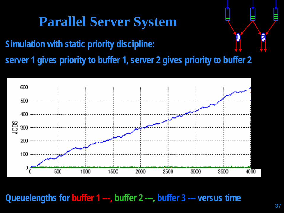
Parallel Server System
Simulation with static priority discipline:
server 1 gives priority to buffer 1, server 2 gives priority to buffer 2
Queuelengths for buffer 1 ---, buffer 2 ---, buffer 3 --- versus time

38
Parallel Server System
Simulation with dynamic priority discipline:
server 1 gives priority to buffer 1, server 2 gives priority to buffer 2, except when queue 2 goes below threshold of size 10
Queuelengths for buffer 1 ---, buffer 2 ---, buffer 3 --- versus time

39
NEXT TWO LECTURES
! Open Multiclass HL Queueing Networks: Stability and Performance
! Control of Stochastic Processing Networks: Some Theory and Examples

40