what is the true shape of a disease cluster? the multi-objective genetic scan luiz duczmal ricardo...
TRANSCRIPT

What is the true shape of a disease cluster? The multi-objective genetic scan
Luiz Duczmal
Ricardo C.H. Takahashi
André L.F. Cançado
Univ. Federal Minas Gerais, Brazil, Statistics Dept., Electrical Engineering Dept., Mathematics Dept.
Geoinfo 2006

Irregularly shaped spatial disease clusters occur commonly in epidemiological studies, but their geographic delineation is poorly defined.
Most current spatial scan software usually displays only one of the many possible cluster solutions with different shapes, from the most compact round cluster to the most irregularly shaped one, corresponding to varying degrees of penalization parameters imposed to the freedom of shape.
Even when a fairly complete set of solutions is available, the choice of the most appropriate parameter setting is left to the practitioner, whose decision is often subjective.

We propose quantitative criteria for choosing the best cluster solution, through multi-objective optimization, by finding the Pareto-set in the solution space.
Two competing objectives are involved in the search: regularity of shape, and scan statistic value.
Instead of running sequentially a cluster finding algorithm with varying degrees of penalization, the complete set of solutions is found in parallel, employing a genetic algorithm.

The cluster significance concept is extended for this set in a natural and unbiased way, being employed as a decision criterion for choosing the optimal solution.
The Gumbel distribution is used to approximate the empiric scan statistic distribution, speeding up the significance estimation.
The method is fast, with good power of detection.
An application to breast cancer clusters is discussed.
Keywords: spatial scan statistic, disease clusters, geometric compactness penalty correction, Pareto-sets, multi-objective optimization, vector optimization, Gumbel distribution, genetic algorithm.
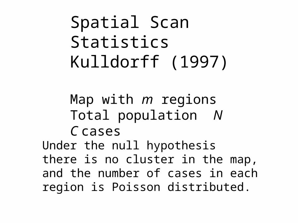
Spatial Scan StatisticsKulldorff (1997)
Map with m regionsTotal population NC cases
Under the null hypothesis there is no cluster in the map, and the number of cases in each region is Poisson distributed.

For each circle centered in each centroid’s region, letz be the collection of regions that lie inside it. Let
= number of cases inside z
= expected cases inside z
zZc
ZZ cC
Z
Z
c
Z
Z
C
cCczL
)(
ZZc if
and one otherwise.
Z
The scan statistic is defined as

The collection (or zone) z with the highest L(z) isthe most likely cluster.
We sweep through all the m2 possible circular
zones, looking for the highest L(z) value.
The whole procedure is repeated for thousandsof times, for each set of randomly distributed cases.(Monte Carlo, Dwass(1957)).
We need to compare this value against the max L(z) for maps with cases distributed randomlyunder the null hypothesis.
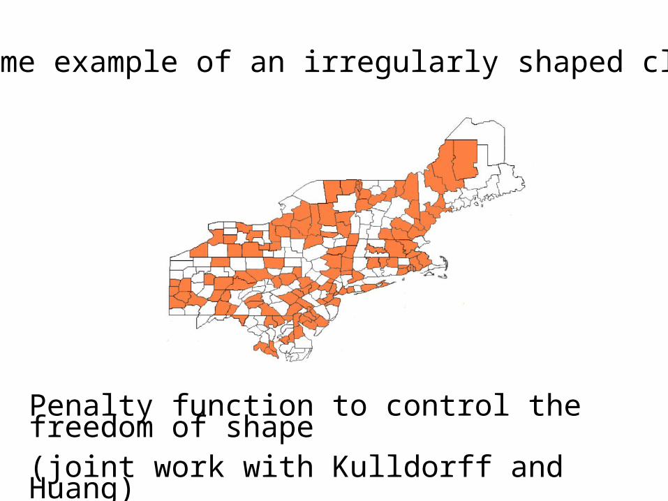
Penalty function to control the freedom of shape (joint work with Kulldorff and Huang)
Extreme example of an irregularly shaped cluster
2)(
)(4)(
zH
zAzK
2
2
)()()(
zH
zAzK
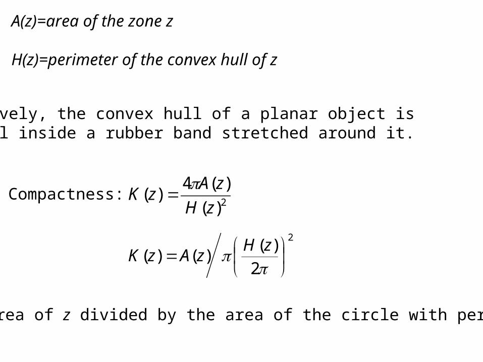
A(z)=area of the zone z
H(z)=perimeter of the convex hull of z
Compactness:
Intuitively, the convex hull of a planar object is the cell inside a rubber band stretched around it.
K(z) = the area of z divided by the area of the circle with perimeter H(z).
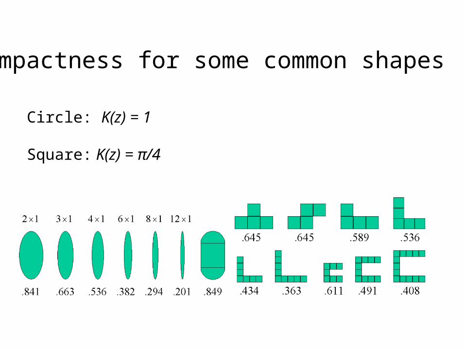
Circle: K(z) = 1
Square: K(z) = π/4
Compactness for some common shapes

Penalty function for the log of the likelihood ratio (LLR(z))
azK )(
K(z).LLR(z)
.LLR(z)
Generalized compactness correction:
a = 1 : full compactness correction
a = 0.5 : medium compactness correction
a = 0.0 : no compactness correction

The Elliptic Scan Statistic(joint work with Kulldorff, Huang and Pickle)
The scanning window has variable location,size, shape and angle. A penalty function may be used.
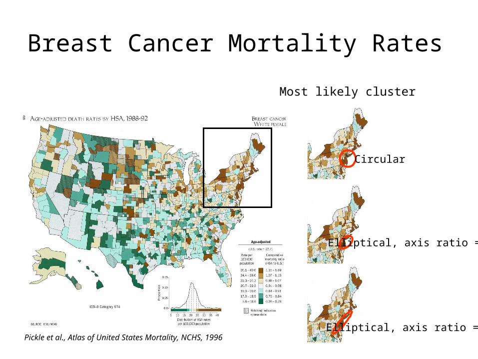
Breast Cancer Mortality Rates
Most likely cluster
Pickle et al., Atlas of United States Mortality, NCHS, 1996
Circular
Elliptical, axis ratio = 2
Elliptical, axis ratio = 5

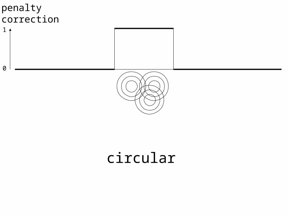
penaltycorrection
1
0
circular
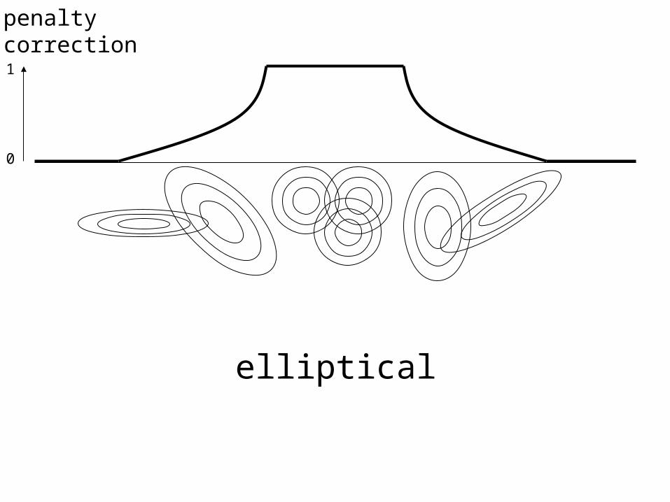
penaltycorrection
1
0
elliptical

penaltycorrection
1
0
irregular
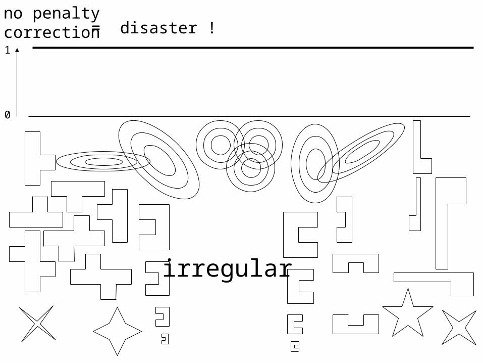
no penaltycorrection
1
0
= disaster !
irregular
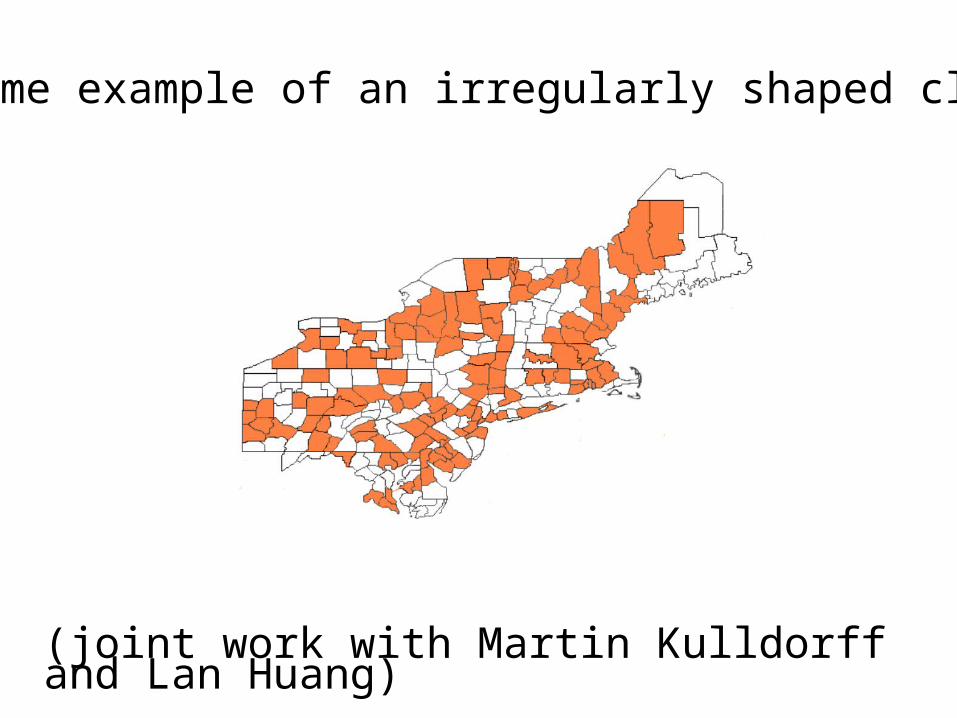
(joint work with Martin Kulldorff and Lan Huang)
Extreme example of an irregularly shaped cluster
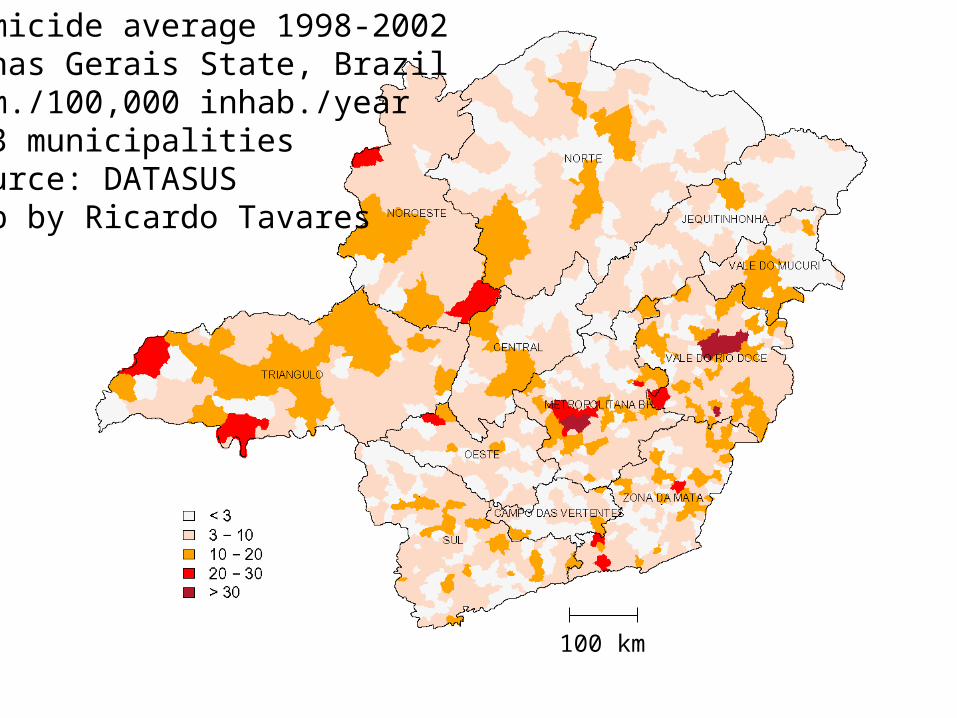
Homicide average 1998-2002Minas Gerais State, BrazilHom./100,000 inhab./year853 municipalitiesSource: DATASUSMap by Ricardo Tavares
100 km
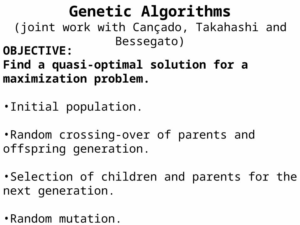
OBJECTIVE:Find a quasi-optimal solution for a maximization problem.
•Initial population.
•Random crossing-over of parents and offspring generation.
•Selection of children and parents for the next generation.
•Random mutation.
•Repeat the previous steps for a predefined number of generations or until there is no improvement in the functional.
Genetic Algorithms(joint work with Cançado, Takahashi and Bessegato)

We minimize the graph-related operations by means of a fast offspring generation and evaluation of the Kulldorff´s scan likelihood ratio statistic.
This algorithm is more than ten times faster and exhibits less variance compared to a similar approach using simulated annealing, and thus gives better confidence intervals for the Monte Carlo inference process of significance evaluation for the most likely cluster found.


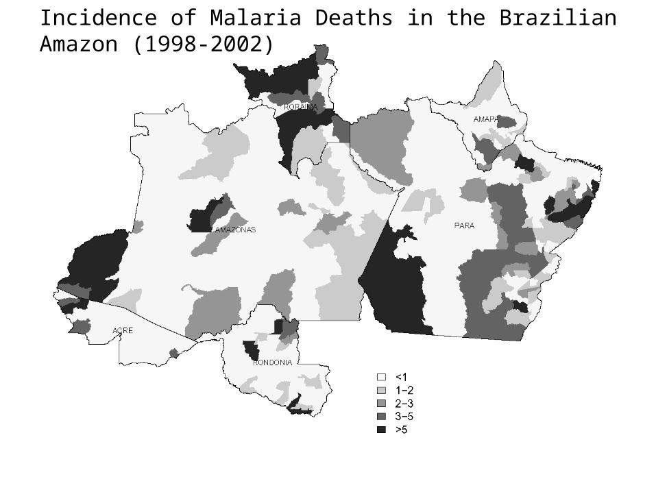
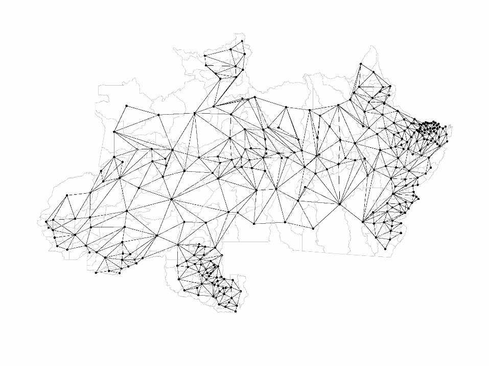
Incidence of Malaria Deaths in the Brazilian Amazon (1998-2002)
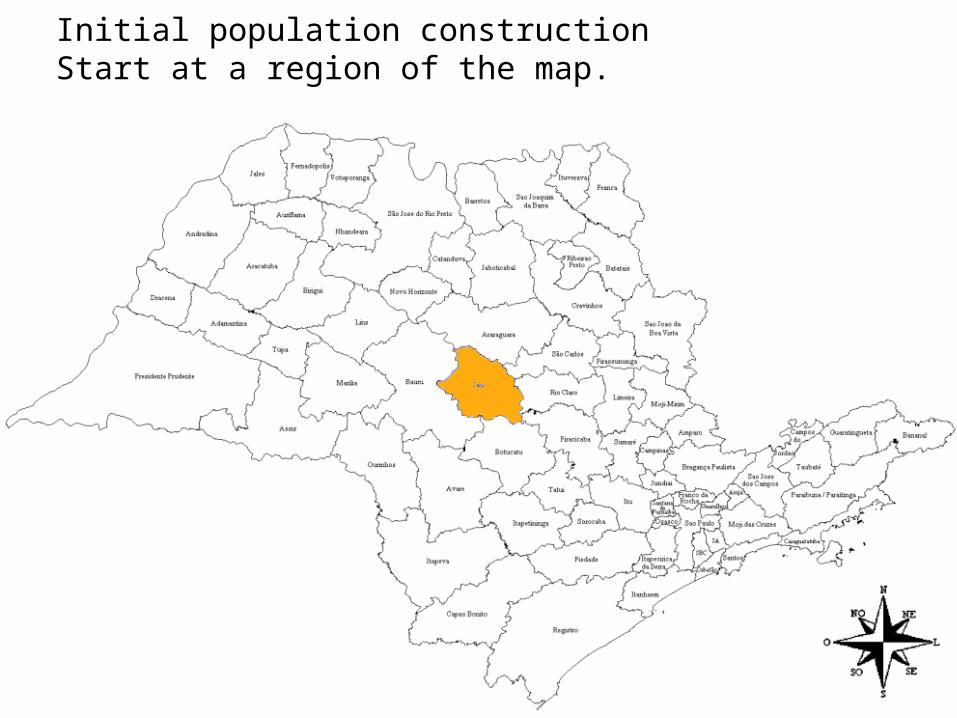
Initial population constructionStart at a region of the map.

Initial population constructionAdd the neighbor which forms the highest LLR 2-cell zone.
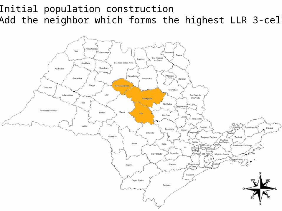
Initial population constructionAdd the neighbor which forms the highest LLR 3-cell zone.

Initial population constructionAdd the neighbor which forms the highest LLR 4-cell zone.

Initial population constructionStop. (It is impossible to form a higher LLR 5-cell zone)
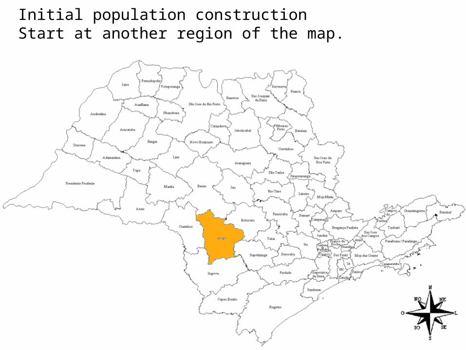
Initial population constructionStart at another region of the map.

Initial population constructionAdd the neighbor which forms the highest LLR 2-cell zone.

Initial population constructionetc.Repeat the previous steps for all the regions of the map.

THE OFFSPRING GENERATION(a simple example)

THE OFFSPRING GENERATION(a simple example)
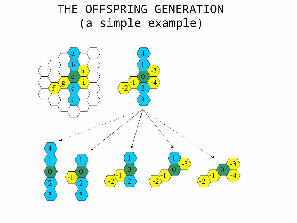
THE OFFSPRING GENERATION(a simple example)
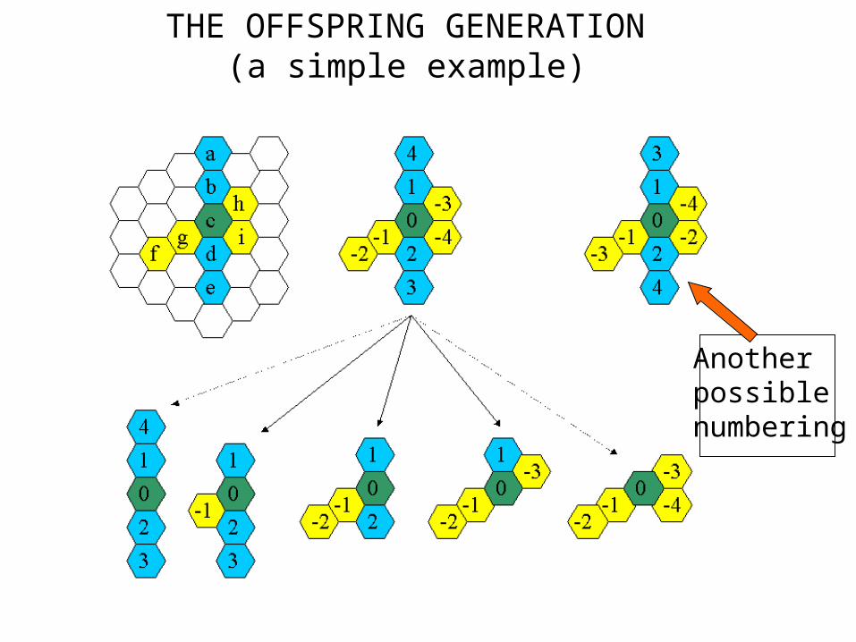
THE OFFSPRING GENERATION(a simple example)
Anotherpossiblenumbering

THE OFFSPRING GENERATION(a more sofisticated example)
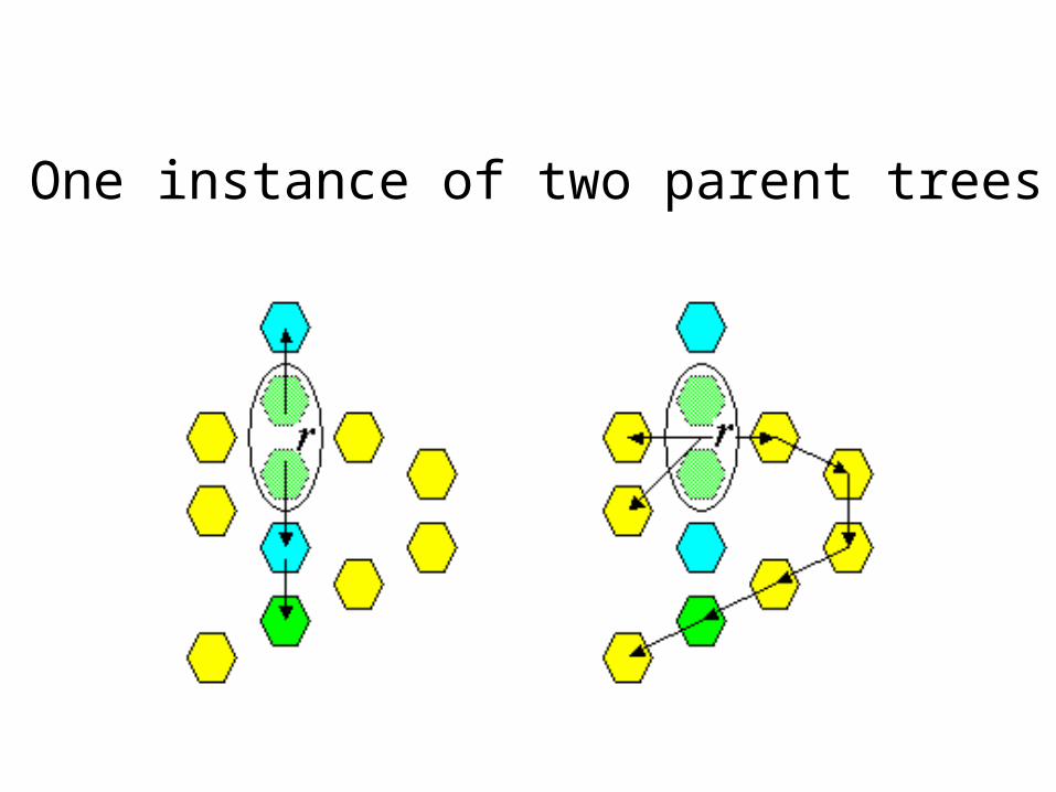
One instance of two parent trees
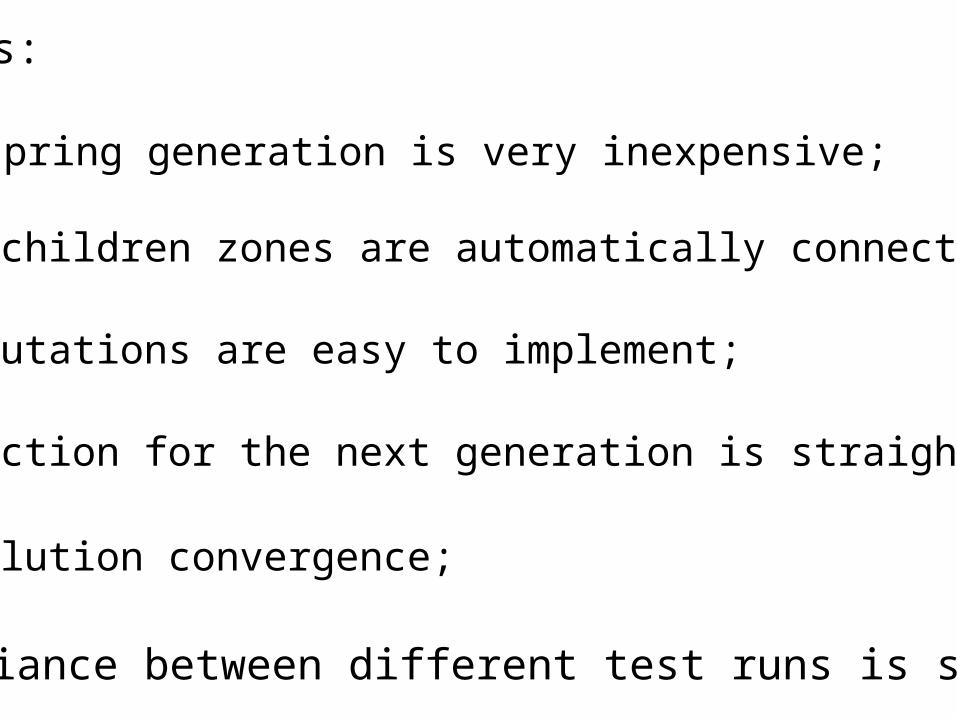
Advantages:
• The offspring generation is very inexpensive;
• All the children zones are automatically connected;
• Random mutations are easy to implement;
• The selection for the next generation is straightforward;
• Fast evolution convergence;
• The variance between different test runs is small.

Population Evolution Performance
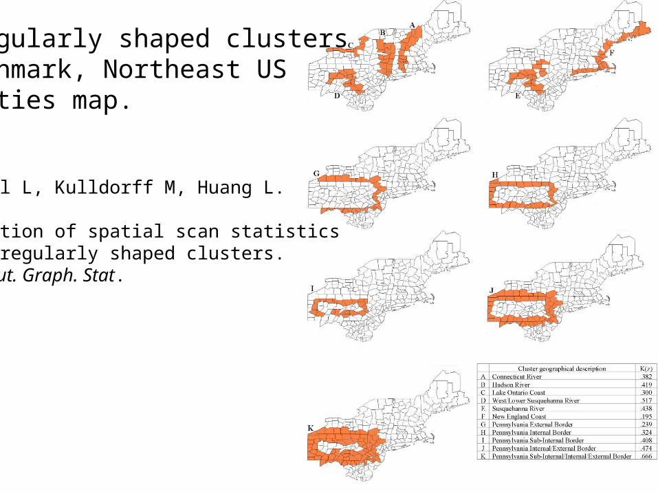
Irregularly shaped clustersbenchmark, Northeast US counties map.
Duczmal L, Kulldorff M, Huang L. (2006) Evaluation of spatial scan statistics for irregularly shaped clusters. J. Comput. Graph. Stat.

Power evaluation of the genetic algorithm, compared to the simulated annealing algorithm.
cluster size penalty G (SA) [8] G (SA) [12] G (SA) [20] G (SA) [30]
A 13 a=0 a=1
.84 (.87)
.85 (.86) .84 (.86) .85 (.86)
.79 (.79)
.84 (.84) .68 (.66) .80 (.79)
B 16 a=0 a=1
.81 (.83)
.81 (.78) .82 (.84) .84 (.84)
.80 (.81)
.86 (.86) .74 (.74) .84 (.83)
C 7 a=0 a=1
.87 (.87)
.80 (.79) .86 (.84)
.78 (.79) .82 (.77) .74 (.74)
.72 (.65)
.68 (.65)
D 15 a=0 a=1
.88 (.89)
.86 (.85) .89 (.90) .89 (.89)
.87 (.88)
.90 (.90) .81 (.81) .87 (.87)
E 21 a=0 a=1
.83 (.82)
.77 (.72) .86 (.85) .82 (.81)
.87 (.87)
.86 (.86) .84 (.84) .87 (.85)
F 23 a=0 a=1
.54 (.58) .45 (.44)
.58 (.61)
.46 (.45) .57 (.59) .48 (.46)
.50 (.51)
.44 (.44)
G 26 a=0 a=1
.58 (.61)
.50 (.49) .62 (.63) .53 (.52)
.66 (.62)
.55 (.52) .68 (.59) .55 (.50)
H 29 a=0 a=1
.66 (.69)
.64 (.62) .67 (.70) .66 (.67)
.70 (.69)
.67 (.67) .69 (.67) .64 (.64)
I 23 a=0 a=1
.66 (.65)
.62 (.59) .71 (.67) .64 (.64)
.74 (.69)
.68 (.66) .71 (.67) .70 (.65)
J 55 a=0 a=1
.58 (.60)
.56 (.54) .64 (.66) .62 (.63)
.69 (.69)
.68 (.67) .72 (.70) .68 (.67)
K 78 a=0 a=1
.53 (.51)
.47 (.43) .61 (.60) .56 (.55)
.69 (.68)
.67 (.66) .75 (.72) .72 (.71)

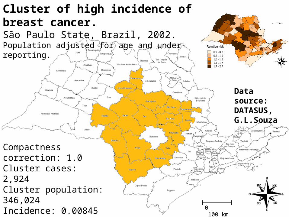
Cluster of high incidence of breast cancer. São Paulo State, Brazil, 2002. Population adjusted for age and under-reporting.
0 100 km
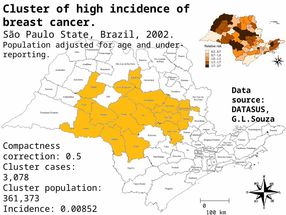
Cluster of high incidence of breast cancer. São Paulo State, Brazil, 2002. Population adjusted for age and under-reporting.
Compactness correction: 1.0 Cluster cases: 2,924Cluster population: 346,024Incidence: 0.00845LLR: 298.9p-value:0.001
Data source: DATASUS, G.L.Souza
0 100 km
Compactness correction: 0.5 Cluster cases: 3,078Cluster population: 361,373Incidence: 0.00852LLR: 343.8p-value:0.001
Data source: DATASUS, G.L.Souza
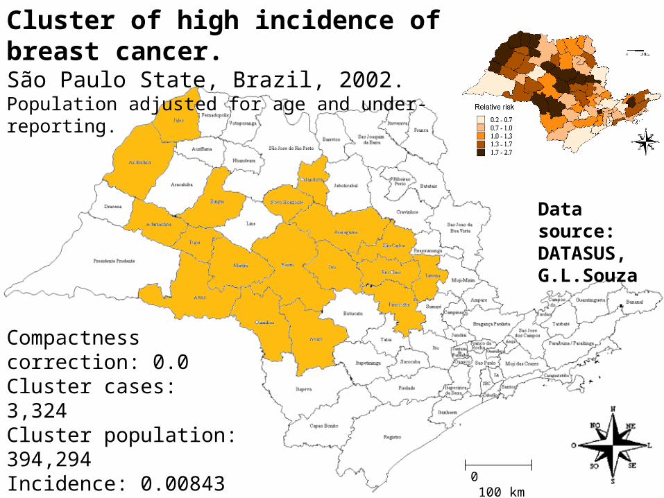
Cluster of high incidence of breast cancer. São Paulo State, Brazil, 2002. Population adjusted for age and under-reporting.
0 100 km
Compactness correction: 0.0 Cluster cases: 3,324Cluster population: 394,294Incidence: 0.00843LLR: 449.6p-value:0.001
Data source: DATASUS, G.L.Souza
Cluster of high incidence of breast cancer. São Paulo State, Brazil, 2002. Population adjusted for age and under-reporting.

• The genetic algorithm for disease cluster detection is fast and exhibits less variance compared to similar approaches;
• The potential use for epidemiological studies and syndromic surveillance is encouraged;
• The need of penalty functions for the irregularity of cluster’s shape is clearly demonstrated by the power evaluation tests;
• The power of detection of clusters is similar to the simulated annealing algorithm;
• The flexibility of shape control gives to the practitioner more insight of the geographic cluster delineation.
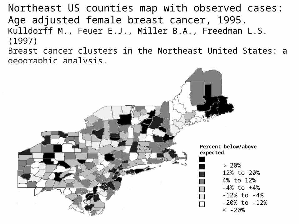
Northeast US counties map with observed cases: Age adjusted female breast cancer, 1995. Kulldorff M., Feuer E.J., Miller B.A., Freedman L.S. (1997) Breast cancer clusters in the Northeast United States: a geographic analysis. American Journal of Epidemiology, 146:161-170.
Percent below/above expected
> 20% 12% to 20% 4% to 12% -4% to +4% -12% to -4% -20% to -12% < -20%
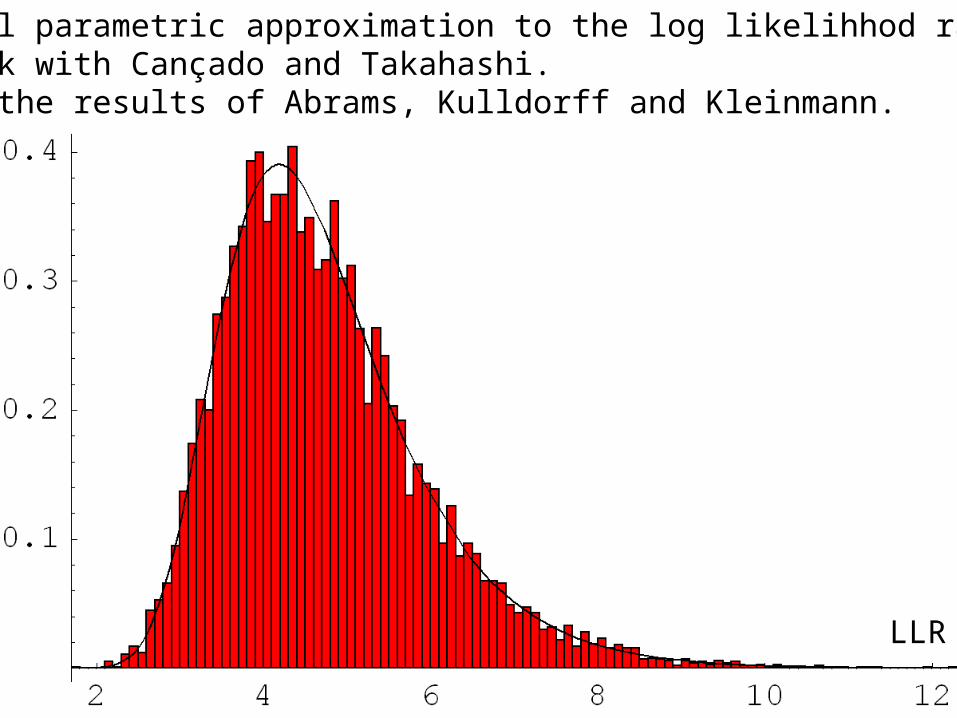
The Gumbel parametric approximation to the log likelihhod ratio scan.Joint work with Cançado and Takahashi.Based on the results of Abrams, Kulldorff and Kleinmann.
LLR

Pareto Sets
The detection of irregularly shaped disease clusters through multi-objective optimization.

The genetic algorithm is used to maximize two objectives:
-the scan statistic.
-the regularity of shape (compactness).

log likelihood ratio
compactness
Elite (red dots):Each red dot is not surpassed by any other point on all variables simultaneously.

log likelihood ratio
compactness
Elite (red dots):Each red dot is not surpassed by any other point on all variables simultaneously.

log likelihood ratio
compactness
Elite (red dots):Each red dot is not surpassed by any other point on all variables simultaneously.

log likelihood ratio
compactness
Elite (red dots):Each red dot is not surpassed by any other point on all variables simultaneously.

log likelihood ratio
compactness
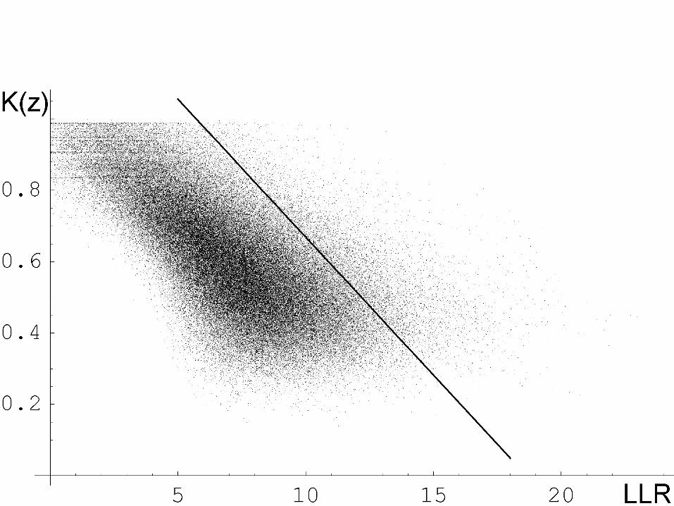
The Pareto Surface is formed joining the elite points.


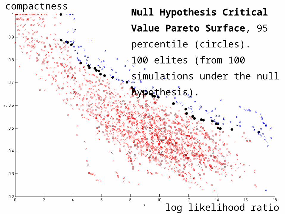
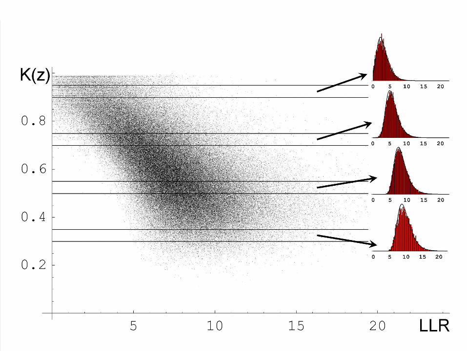
Null Hypothesis Critical Value
Pareto Surface, 95 percentile (circles).
100 elites (from 100 simulations under
the null hypothesis).
log likelihood ratio
compactness
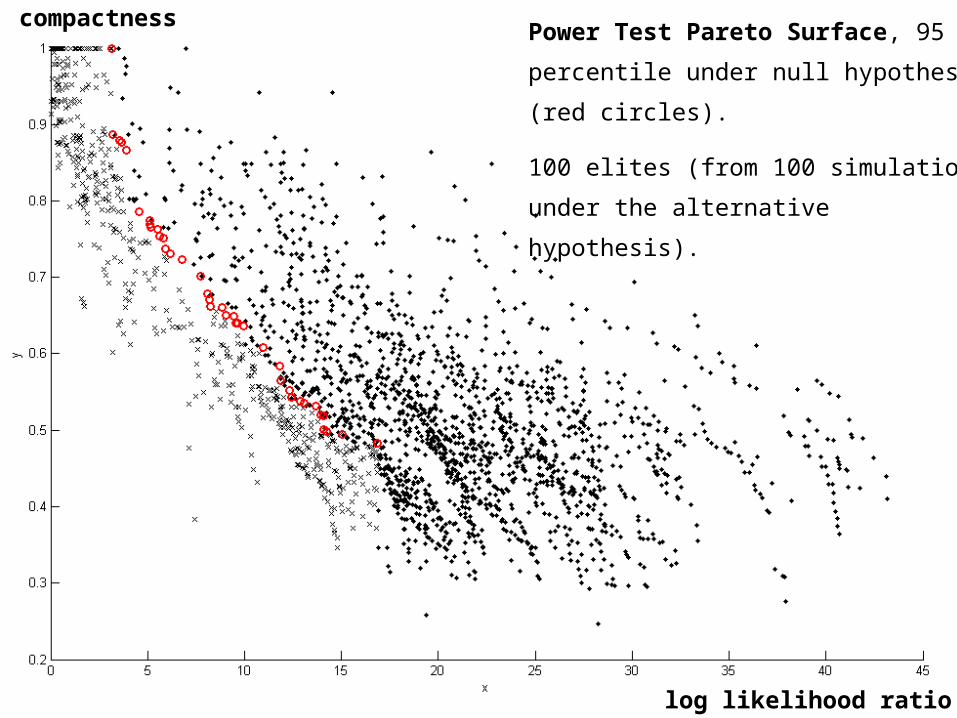
compactness
log likelihood ratio
Power Test Pareto Surface, 95 percentile
under null hypothesis (red circles).
100 elites (from 100 simulations under the
alternative hypothesis).


Northeast US counties map with observed cases: Age adjusted female breast cancer, 1995. Kulldorff M., Feuer E.J., Miller B.A., Freedman L.S. (1997) Breast cancer clusters in the Northeast United States: a geographic analysis. American Journal of Epidemiology, 146:161-170.
Percent below/above expected
> 20% 12% to 20% 4% to 12% -4% to +4% -12% to -4% -20% to -12% < -20%


Duczmal L, Kulldorff M, Huang L. (2006) Evaluation of spatial scan statistics for irregularly shaped clusters. J. Comput. Graph. Stat. 15;2,1-15.Duczmal L, Cançado ALF, Takahashi RHC, Bessegato LF, 2006. A genetic algorithm for irregularly shaped spatial scan statistics (submitted).Duczmal L, Cançado ALF, Takahashi RHC, 2006. Delineation of Irregularly Shaped Disease Clusters through Multi-Objective Optimization (submitted). Duczmal L, Assunção R. (2004), A simulated annealing strategy for the detection of arbitrarily shaped spatial clusters, Comp. Stat. & Data Anal., 45, 269-286. Kulldorff M, Huang L, Pickle L, Duczmal L. (2005) An Elliptic Spatial Scan Statistic. Statistics in Medicine (to appear). Patil GP, Taillie C. (2004) Upper level set scan statistic for detecting arbitrarily shaped hotspots. Envir. Ecol. Stat., 11, 183-197. Kulldorff M. (1997), A Spatial Scan Statistic, Comm. Statist. Theory Meth., 26(6), 1481-1496. Kulldorff M, Tango T, Park PJ. (2003) Power comparisons for disease clustering sets, Comp. Stat. & Data Anal., 42, 665-684. Kulldorff M, Feuer EJ, Miller BA, Freedman LS. (1997) Breast cancer clusters in the Northeast United States: a geographic analysis. Amer. J. Epidem., 146:161-170. de Souza Jr. GL (2005) The Detection of Clusters of Breast Cancer in São Paulo State, Brazil. M.Sc. Dissertation, Univ. Fed. Minas Gerais.
References