what does monetary policy do? - brookings does monetary policy do? there is a long tradition in...
TRANSCRIPT

ERIC M. LEEPER Indiana University
CHRISTOPHER A. SIMS Yale University
TAO ZHA Federal Reserve Bank of Atlanta
What Does Monetary Policy Do?
THERE IS A long tradition in monetary economics of searching for a single policy variable-perhaps a monetary aggregate, perhaps an in- terest rate-that is more or less controlled by policy and stably related to economic activity. Whether the variable is conceived of as an indi- cator of policy or a measure of policy stance, correlations between the variable and macroeconomic time series are taken to reflect the effects of monetary policy. Conditions for the existence of such a variable are stringent. Essentially, policy choices must evolve autonomously, in- dependent of economic conditions. Even the harshest critics of mone- tary authorities would not maintain that policy decisions are unrelated to the economy. In this paper we extend a line of work that builds on a venerable economic tradition to emphasize the need to specify and estimate behavioral relationships for policy. The estimated relationships separate the regular response of policy to the economy from the re- sponse of the economy to policy, producing a more accurate measure of the effects of policy changes.
The views expressed here are not necessarily those of the Board of Governors of the Federal Reserve System or the Federal Reserve Bank of Atlanta. The authors would like to acknowledge what they have learned about the implementation of monetary policy from conversations with Lois Berthaume, Will Roberds, and Mary Rosenbaum of the Federal Reserve Bank of Atlanta, Charles Steindel of the Federal Reserve Bank of New York, Marvin Goodfriend of the Federal Reserve Bank of Richmond, and Sheila Tschin- kel. David Petersen of the Federal Reserve Bank of Atlanta helped both in locating data and in discussing the operation of the money markets.
1

2 Brookings Papers on Economic Activity, 2:1996
One sometimes encounters the presumption that models for policy analysis and those for forecasting are sharply distinct: a model that is useful for policy choice need not fit the data well, and well-fit models necessarily sacrifice economic interpretability. We do not share this presumption and aim to show that it is possible to construct economi- cally interpretable models with superior fit to the data.
As the recent empirical literature on the effects of monetary policy has developed ways of handling more complex, multivariate data sets, a variety of new models and approaches has emerged. Researchers have chosen different data sets, made different assumptions, and tended to emphasize the differences between their results and those of others, rather than the commonalities. This paper uses a single time frame and data set to check the robustness of results in the literature and to trace the nature and sources of the differences in conclusions.
We analyze and interpret the data without imposing strong economic beliefs. The methods that we employ permit estimation of large time- series models and thus more comprehensive analysis of the data. The models integrate policy behavior variously with the banking system, with demand for a broad monetary aggregate, and with a rich array of goods and financial market variables to provide a fuller understanding of the mechanism of monetary transmission. The combination of weak economic assumptions and large models reveals difficulties of distin- guishing policy effects, which other approaches fail to bring out.
The size of the effects attributed to shifts in monetary policy varies across specifications of economic behavior. We show that most of the specifications imply that only a modest portion (in some cases, essen- tially none) of the variance in output or prices in the United States since 1960 can be attributed to shifts in monetary policy. Furthermore, we point out substantive problems in the models that imply large real effects on output or prices and argue that correcting these reduces the implied size of the real effects.
Another robust conclusion, common across these models, is that a large fraction of the variation in monetary policy instruments can be attributed to the systematic reaction of policy authorities to the state of the economy. This is what one would expect of good monetary policy, but it is also the reason why it is difficult to use the historical behavior of aggregate time series to uncover the effects of monetary policy.
Eric M. Leeper, Christopher A. Sims, and Tao Zha 3
Method
We use a class of models called identified vector autoregressions (VARs) that has only recently begun to be widely used. Nonetheless, much of the previous empirical research on the effects of monetary policy uses methods that fit within this general framework. In this section we describe the framework, summarize how it differs from other popular frameworks, and consider some common criticisms. In the following section we discuss the ways in which we and others have put substantive meat on this abstract skeleton.
Model Form and Identification
Identified vector autoregressions break up the variation in a list of time series into mutually independent components, according to the following general scheme. If y(t) is a (k x 1) vector of time series, we write
in
(1) , A,y(t - s) = A(L)y(t) = e(t), s=o
where L is a lag operator and the disturbance vector E(t) is uncorrelated with y(s) for s < t and has an identity covariance matrix. I We assume that AO is invertible, which guarantees that one can solve equation 1 to produce
t-I
(2) y(t) = E CsE(t - s) + Eoy(t). s=o
The elements of Cs, treated as functions of s, are known as the model's impulse responses because they delineate how each variable in y re- sponds over time to each disturbance in E.2
1 Note that we have omitted any constant terms in the system. There is no loss of generality if ones admits the possibility that one of the equations takes the form yk(t) = Yk(t - 1), with no error term, in which case Yk becomes the constant.
2. We write as if we were sure that a correct model can be constructed in the form of equations 1 and 2 with our list of variables. If we have omitted some important variable, this assumption may be incorrect. A related, but technically more subtle point is made by Sargent (1984), who notes that it is possible for a representation of the form

4 Brookings Papers on Economic Activity, 2:1996
To use this mathematical structure for economic policy analysis, one has to identify it-give its elements economic interpretations.3 The mathematical model explains all variation in the data as arising from the independent disturbances, E. Since we are studying the effects of monetary policy, we need to specify an element of the E vector, or a list of its elements, that represents disturbances to monetary policy. The equation system 1 contains one equation for each element of the E
vector, defining it as a function of current and past values of y(t). So specifying the element or elements of E that correspond to monetary policy is equivalent to specifying an equation or set of equations that characterizes monetary policy behavior. These equations can be thought of as describing relations among current and past values of y that hold exactly when there are no disturbances to policy. They are, in other words, policy rules or reaction functions. The remaining equations of the system describe the nonpolicy part of the economy, and their dis- turbances are nonpolicy sources of variation in the economy.
While representations of the behavior of the y time series in the form of equations 1 and 2 exist under fairly general conditions, they are not unique. Models in this form with different A and (therefore) C coeffi- cients may imply exactly the same behavior of y. Because the impli- cations of a change in monetary policy are determined by A and C, this means that models with different policy implications may be indistin- guishable on the basis of their fit to the data. When this is true, the model is said to be unidentified. The nature of the indeterminacy is as follows. Given any matrix W satisfying W'W = I (that is, any ortho- normal matrix), one can replace E by WE, A(L) by WA(L), and C(L) by
(2) to exist for a list of variables even though the corresponding form (1) may not be available. This occurs when C in equation 2 is not what engineers call a minimum delay filter. Intuitively, it occurs when the variables in y do not respond quickly enough to E. While this is important, it is really a special case of the initial point that one can obtain misleading results by not having the right list of variables.
3. "Identify" is used in various senses in economics. Sometimes, as in this para- graph, an identified model is one that has an economic interpretation, as opposed to a reduced form model that merely summarizes the statistical properties of the data. But at other times, a model is said to be identified only when the data to be used in fitting it are informative about its behavioral interpretation. Often, but not always, in these situations, more than one behavioral interpretation can be given to the same reduced form. In this paper we follow common practice by choosing the meaning, depending on the context.

Eric M. Leeper, Christopher A. Sims, and Tao Zha 5
C(L)W', arriving at a new representation of the same form. Since the new version of the model is just a linear transformation of the old, it implies the same time-series properties for the data, y. Only if one knows enough about the form of A (or, equivalently, C) to rule out some transformed WAs or CWs as implausible or impossible can the data lead to the most likely form of A.
We use three sorts of identifying restrictions to pin down the con- nection between A and the implied behavior of y. First, we use exact linear restrictions on the elements of AO, usually simply setting certain elements to zero. To rely entirely on these restrictions, one would need at least k[(k - 1)/2] of them, because a (k x k) orthonormal matrix has this many free parameters. With this number of restrictions on the elements of AO. the restriction equations, together with the k[(k - 1)/2] independent restrictions in the W'W = I requirement, are suffi- cient in number to make W unique.4 We also use probabilistic assertions about elements of A-that certain values or relations among values of elements of A are more likely than others. And third, we use informal restrictions on the reasonableness of the impulse responses, the Cs in equation 2. The first two types are easy to handle mathematically, but the latter is not. We use it informally, in that we focus attention on results that do not produce implausible impulse responses. Our criterion for plausibility is loose. We do not expect to see strongly positive responses from prices, output, or monetary aggregates to monetary contraction, nor strongly negative responses from interest rates. Our informal use of this sort of identifying information may give the impres- sion of undisciplined data mining. We could have accomplished the same, at much greater computational cost, by imposing our beliefs about the forms of impulse responses as precise mathematical restric- tions, but this would not have been any more "disciplined." Our pro- cedure differs from the standard practice of empirical researchers in economics only in being less apologetic. Economists adjust their models until they both fit the data and give "reasonable" results. There is nothing unscientific or dishonest about this. It would be unscientific or
4. This is an order condition, analogous to that used for identification in simultaneous equations (SE) modeling. As in SE modeling, there is always a possibility that although there are enough equations, they are not independent, so that a rank condition fails while an order condition holds.

6 Brookings Papers on Economic Activity, 2:1996
dishonest to hide results for models that fit much better than the one presented (even if the hidden model seems unreasonable), or for models that fit about as well as the one reported and support other interpreta- tions of the data that some readers might regard as reasonable. We do nothing of this sort.
Our approach to identification in this paper is very similar to that followed in the rest of the identified VAR literature, but it differs from some other approaches to quantitative macroeconomics. In some cases, the differences correspond to common criticisms of the identified VAR approach by the advocates of those other approaches.
Comparisons with Other Approaches
Traditional econometric simultaneous equations (SE) modeling works with systems quite similar in form to those that we deal with. It begins with a system in the form of equation 1, usually with our as- sumption that the E vector is uncorrelated across time, and always without our assumption that E has an identity covariance matrix. With an unrestricted Ql as a covariance matrix for E, the mathematical struc- ture is subject to a wider range of transformations that leave the model's implications for data unchanged. While the identified VAR framework admits an arbitrary orthonormal W as a transformation matrix, the stan- dard SE framework admits an arbitrary nonsingular matrix V in the same role. So in order to pin down the mapping between E and the data, the SE approach requires stronger a priori restrictions on A. Tradition- ally these have taken two forms. One is block triangularity restrictions on contemporaneous interactions among variables (A, from equation 1) that are linked to conformable block diagonality restrictions on fQ. Such a combination breaks the variable list into two components, usually labeled predetermined and endogenous, respectively. The second form of restriction adds linear constraints (again, often simply setting coef- ficients to zero) on the elements of the rows of A corresponding to the endogenous variables.
To get a feeling for the differences in the requirements for identifi- cation between identified VARs and traditional simultaneous equations, it may help to consider the simplest model. In a two-equation system with no lags, a single zero restriction on A, suffices for identification in the identified VAR framework. That is, the system

Eric M. Leeper, Christopher A. Sims, and Tao Zha 7
(3) a,y,(t) + al2y2(t) = E,(t)
a22y2(t) = E2(t)
in which we have imposed the single constraint a21 = 0, has a unique mapping from A to the stochastic properties (here, simply the covari- ance matrix) of y. The y vector is implied to have a covariance matrix Q = (AO'AO)- i, and AO can be found from fl as the inverse of its unique upper triangular square root, or Choleski decomposition. If equation 3 is interpreted as a traditional simultaneous equations system, however, it is not identified-arbitrary linear combinations of the two equations satisfy all the restrictions (since there are none) on the form of the first equation, while leaving the implications of the system for the behavior of y unchanged. A nonsingular linear transformation of the system can replace the first equation with a linear combination of the two equations, while leaving the second equation unchanged. An orthonormal linear transformation must change both equations at once in order to preserve the lack of correlation between the disturbances. This is why the system is not identified as a standard SE model, but is identified as our type of identified VAR model. Called recursive, this kind of system is a well- recognized special case in the simultaneous equations literature.5 In this two-variable version, a single linear restriction on any of the four coef- ficients in AO, together with the usual identified VAR restriction that the es are uncorrelated, is equivalent to the assumption in traditional SE modeling that one of the variables in the system is predetermined.
Impulse responses can be computed for traditional SE models as well as for identified VARs. In an identified VAR, though, the restriction that Var(E) = I means that, in some circumstances, conclusions about model behavior are less dependent on identifying assumptions about A than in SE models. Consider an example from the discussion below. One might find that the rows of C(L) that correspond to prices and interest rates (the first and second rows, say) mostly show prices and interest rates moving in the same direction, when they show any sub- stantial movement: c,j(s) and c2j(s) have the same sign for most values of j and s when either clj(s) or c,j(s) is large. One might expect that the response to a monetary policy shock should show the opposite sign pattern-c,j(s) and C2j(S) would move in opposite directions. Then one
5. See, for example, Theil (1971, ch. 9).

8 Brookings Papers on Economic Activity, 2:1996
could conclude that monetary policy disturbances cannot account for much of the observed variation in prices and interest rates, regardless of the specific identifying restrictions. It is true that linear transforma- tions of the system will correspond to linear transformations of the disturbances. Some linear transformations (differences, for example) of responses that have c,j(s) and c2j(s) of the same sign could easily show c,j(s) and c2j(s) of opposite signs. But orthonormal transforma- tions of responses that all show large movements of clj(s) and c2j(s) with the same sign cannot produce transformed responses that are both of the opposite sign and also large. In other words, if most of the disturbances that produce substantial interest rate responses show sub- stantial price movements in the same direction, then it is characteristic of the data that these two variables tend to move in the same direction. A monetary policy disturbance, which moves the two variables in op- posite directions, cannot then be accounting for more than a small part of overall variance in interest rates. One could not reach the same conclusion from a traditional SE model, because one would have to admit the possibility of a monetary policy shock with large variance, offset by another shock that also moves prices and interest rates in opposite directions but is negatively correlated with the monetary disturbance.
This brings out one advantage of insisting that a well-specified model account for all correlations among disturbances, so that the disturbances have an identity covariance matrix. When the historical record shows a very strong pattern of positive comovement between interest rates and prices, if one believes that monetary policy disturbances would generate negative comovements, it is reasonable to conclude that monetary pol- icy disturbances have not been a major source of variation in the data. It seems strained to insist that monetary policy disturbances could be important, but tend to be systematically offset by simultaneous private sector disturbances. If this is actually the case, it raises questions about the model. Do the offsetting private sector shocks occur because of an effect of monetary policy on the private sector shocks? If so, our model implies that once the full effects of a monetary policy disturbance are accounted for, it does not move interest rates and prices in opposite directions, which is suspicious. Do the offsetting shocks arise because of an effect of the private sector on policymaking? If so, this ought to be taken into account in the model of policy behavior.

Eric M. Leeper, Christopher A. Sims, and Tao Zha 9
Objections to Identified VAR Modeling
It is sometimes suggested that disturbances are what is "omitted from the theory," and that therefore one cannot claim to know much about their properties. Note, though, that traditional assumptions of predetermination make the same kinds of assertions about the lack of correlation among sources of variation as identified VAR models. If one really knows nothing about the stochastic properties of disturbance terms, one will not be able to distinguish disturbances from systematic components of variation. Furthermore, correlation among disturbances is a serious embarrassment when a model is actually used for policy analysis. If disturbances to the monetary policy reaction function are strongly correlated with private sector disturbances, how can one use the system to simulate the effects of variations in monetary policy? In practice, the usual answer is that simulations of the effects of paths of policy variables or of hypothetical policy rules are conducted under the assumption that such policy changes can be made without producing any change in disturbance terms in other equations, even if the esti- mated covariance matrix of disturbances shows strong correlations. This is not logically inconsistent, but it amounts to the claim that the true policy disturbance is that part of the reaction function residual that is not correlated with other disturbances in the system. This, in turn, is equivalent to claiming that the true reaction function is a linear com- bination of what the model labels the reaction function and the other equations in the system whose disturbances are correlated with it. Our view is that if one is going to do this in the end, the assumptions on the model that justify doing so should be explicit from the beginning.
Advocates of traditional SE models are also sometimes puzzled by the focus on policy shocks (the E vector) in the identified VAR ap- proach. This is largely a semantic confusion. As we point out above, identifying policy shocks is equivalent to identifying equations for pol- icy reaction functions. In addition, distinguishing these shocks from other sources of disturbance to the system is equivalent to identifying the nonpolicy equations of the model, which determine the response of the system to policy actions or to changes in the policy rule. The prominence of shocks in presentations of identified VAR results merely reflects a sharp focus on the model's characteristics as a probability model of the data. In practice, traditional SE approaches often focus
10 Brookings Papers on Economic Activity, 2:1996
on the equations and treat the rest of the stochastic structure casually. Identified VAR results are often presented as tables or charts of re- sponses to shocks, the Cs in equation 2. But these carry exactly the same information about the model as the As in equation 1, the equation coefficients that are more commonly presented in traditional SE mod- eling approaches. Presentations of SE models also often include simu- lations of the model with various kinds of perturbations. The Cs can be thought of as a systematic set of simulations, of responses to a range of types of disturbance that is wide enough to display all aspects of the model's behavior.
Identified VAR models are sometimes faulted, as are SE models, in terms of the rational expectations critique, as follows. Some of the dynamic of these models arises from the formation of the public's expectations. The models have been used to examine the effects of making large, permanent changes in policy rules. The policy equations are replaced by possible new rules, and the remaining equations, which incorporate the public's expectations, are left unchanged. The rational expectations critique points out that such exercises are potentially mis- leading because they contradict the probability structure of the esti- mated model. The model is fit to historical data under the assumption that variation in policy can be accounted for by the model's stochastic disturbances-the additive error terms in the policy reaction functions. In the simulation experiment, quite a different form of policy variation is examined. If such variation is not historically unprecedented, there is a misspecification in the model: something that the model's structure implies is impossible has actually occurred in the past. This contradic- tion invalidates the assumption that the dynamics of expectations for- mation remain stable when the policy rule is changed.
The rational expectations critique reiterates the general principle that caution is necessary in extrapolating models to situations that are far from the history to which they have been fit. Yet to use a model requires applying it to situations that deviate to some extent from past experi- ence. It is interesting and useful to try changing the policy rules equa- tions in a model, holding the other equations fixed, so long as one recognizes that this is just a convenient way of generating a sequence of disturbances to the policy rule originally estimated. Concern about extrapolating the model too far is justified when the implied sequence

Eric M. Leeper, Christopher A. Sims, and Tao Zha 11
of policy disturbances differs substantially by size or serial correlation properties from what has been observed historically.
Although the rational expectations critique was initially formulated as an attack on traditional SE modeling and has also been directed against identified VAR modeling, it actually applies to all forms of macroeconomic modeling. The critique emphasizes that policy should always be modeled as stochastic and that the public's behavior depends on its uncertainty about policy. Therefore one should regard the exer- cise of simulating a model with a policy rule different from what has been fit to history only as one convenient way to generate a sequence of stochastic disturbances to policy.
Another branch of quantitative macroeconomics, the dynamic sto- chastic general equilibrium (DSGE) approach, arose largely as a re- sponse to the rational expectations critique.6 Although advocates of this approach fault traditional SE and identified VAR models for being insufficiently attentive to the rational expectations critique, the methods that have been used to examine the effects of policy under the DSGE approach are equally subject to the critique. The DSGE approach has often embraced the idea that the only kinds of policy changes that are worth studying are those that are historically unprecedented, are com- pletely unexpected by the agents populating the model, and will never be reversed. In this situation, DSGE models do give an internally con- sistent answer as to the effects of the policy change. But the need for caution remains as great as in traditional SE models. Any evidence in the data about the effects of such an unprecedented policy shift has to be entirely indirect-an extrapolation, based on a priori assumptions, to a range of experience beyond that to which the model has been fitted. And the results, despite being internally consistent, are answers to an uninteresting question: DSGE models are usually used in policy analysis to describe the effects of a type of policy change that never in fact occurs. The models that have now evolved from traditional SE models often trace out the effects of nonstochastic shifts in policy reaction functions using rational expectations, as do most DSGE models. Al-
6. The DSGE approach is more commonly known as the real business cycle ap- proach. But while it initially used models without nominal rigidities or any role for monetary policy, the methodology has now been extended to models that include nominal rigidities; see, for example, Jinill Kim (1996).

12 Brookings Papers on Economic Activity, 2:1996
though advocates of the two types of models make very different choices about the trade-offs between model abstraction, internal con- sistency, and fit to the data, the inherent limitations of simulating non- stochastic shifts in policy rules are common to both DSGE and the newer SE-style models.7
Note the common thread in the criticisms of the identified VAR approach from the SE modeling side and the DSGE modeling side: both are uncomfortable about treating policy as random. Some would say that one cannot contemplate improving policy as if one could choose it rationally and, at the same time, think of policy as a random variable. This notion is simply incorrect. Examination of historical policy deci- sions clearly shows that policy pursues multiple objectives in an uncer- tain environment. Economists with the Board of Governors of the Fed- eral Reserve System and the regional Federal Reserve banks collect and analyze a large body of economic information, on which the Federal Open Market Committee bases its decisions. Committee members com- pare staff forecasts of a wide range of macroeconomic variables against their own desired paths for these variables. Each member's policy choice minimizes a loss function, subject to a set of ancillary con- straints, such as a desire to smooth interest rates and avoid disrupting financial markets. Federal Reserve policy is an outgrowth both of the members' economic concerns and of the dynamic interplay among members. The result of this process is surely as random as any other aspect of economic behavior.
When one considers offering advice on current or future policy de- cisions, one would not ordinarily propose to flip a coin, but this does not mean that it is a mistake to think of policy choice as the realization of a random variable. Choices that are made systematically by one person or group are likely to be unpredictable by others. If, in a break with the past, monetary policy were to be set by a single, internally consistent, rational policymaker, the public would be surprised and would most likely remain uncertain for some time that the new pattern would persist. Therefore, even if modeling efforts were addressed to
7. Examples of the newer SE-style models include Bryant (1991), Bryant, Hooper, and Mann (1993), Taylor (1993), and, in principle, the new Federal Reserve Board model described in Brayton and Tinsley (1996). An important design goal of this new model is the ability to simulate both deterministic rule shifts with rational expectations and policy changes modeled as shocks to the existing rule.

Eric M. Leeper, Christopher A. Sims, and Tao Zha 13
this hypothetical unified, rational policymaker, one should model policy choices as the realization of random variables when tracing their impact on the economy.
Policy analysts who work with models generally understand a DSGE- style analysis of nonstochastic changes in policy rule to characterize effects of policy changes in the long run, and analysis of the effects of policy shocks with a fixed reaction function equation to characterize short-run effects.8 This is a reasonable interpretation, by and large. It recognizes that if it is realistic to contemplate changing supposedly nonstochastic coefficients in policy reaction functions, this is a source of inaccuracy in the model and is grounds for caution in long-run extrapolations. It also recognizes that a DSGE-style analysis of policy rule shifts cannot be applied to projecting the effects of policy changes of the type, and over the time horizons, that are the main subject of policy discussion, because it models policy as nonstochastic. Ideally, one would like a model without either limitation, whose stochastic characterization of policy behavior encompassed all the kinds of shifts in policy that one actually considers. In such a model, every interesting and plausible policy change, including those that it seems natural to describe as changes in policy rule, could be expressed as a sequence of shocks to the model's driving random variables. There are a few models in the literature that go some way toward this goal, for example, by modeling policy as switching between linear rules with additive errors, according to some well-defined Markov process. But the analytical difficulties raised by even simple models like this are substantial.
We should add that this sharp contrast between the approach of DSGE modelers to the analysis of policy changes and our own reflects only a difference of practice. There is nothing in principle that ties DSGE models to the approach that researchers have commonly taken when applying them to policy analysis. Indeed, Eric Leeper and Chris- topher Sims, and Jinill Kim present examples of DSGE models in which
8. Another way in which policy analysts sometimes characterize the distinction is to label the effects of policy shocks (with the policy equation coefficients fixed) as the effects of unanticipated policy changes, and the effects of nonstochastic changes in policy rule as the effects of anticipated, or credible, policy changes. We regard this distinction as much less helpful than the long- and short-run distinction. It may encour- age the idea that there is some choice as to whether policy changes will be credible when first announced. In fact, credibility can only arise from a consistent pattern of action.

14 Brookings Papers on Economic Activity, 2:1996
careful attention is paid to modeling the stochastic structure of policy, therefore allowing examination of the effects of both stochastic disturb- ances to policy and deterministic changes in policy rule.9
Nor is there any fundamental conflict between the mathematics of our modeling approach in this paper and that of DSGE models. Our model is linear, whereas most DSGE models are nonlinear; but their nonlinearities are not usually strong. Indeed, one common approach to solving and fitting DSGE models to the data is to take a linear approx- imation to them around a steady state. A linearized DSGE model be- comes a VAR model, with a particular pattern of identifying restrictions on its coefficients. Since linearized DSGE models are generally much more strongly restricted than identified VAR models, there are many fewer free parameters to estimate. However, the kinds of restrictions that are used to identify VAR models are often imposed as a subset of the restrictions used in DSGE models, so that identified VAR models can be thought of as weakly restricted linearized DSGE models.
This is what, in fact, distinguishes the DSGE from the identified VAR modeling approach. The former begins with a complete interpre- tation of each source of stochastic disturbance in the model, invoking many conventional but arbitrary restrictions on functional forms of utility and production functions and on stochastic properties of disturb- ances. The fitted model can tell the full story about how, and by what means, each source of disturbance affects the economy. The identified VAR modeling approach, by contrast, begins with an unidentified time- series model of the economy and introduces identifying information cautiously. The fitted model then fits the data well, usually much better than DSGE models of the same data, but tells only an incomplete story about each source of disturbance. In an identified VAR, many sources of disturbance typically are not completely interpreted, but are merely identified as part of a vector of private sector shocks, for example, that may mix technology shocks and taste shocks. The effects of monetary policy disturbances on the economy may be traced out, but how those effects work their way through the behavior of investors and consumers may not be completely apparent.
Each approach has its advantages and its disadvantages. The identi- fied VAR approach may give a more accurate impression of the degree
9. Leeper and Sims (1994); Jinill Kim (1996).

Eric M. Leeper, Christopher A. Sims, and Tao Zha 15
of uncertainty about the model's results. It also reduces the chance of attributing to the data a result that actually flows almost entirely from initial ad hoc modeling assumptions. At the same time, the identified VAR approach does not provide as convenient a framework for applying a priori knowledge or hypotheses about the structure of the economy.
After considering alternatives to and criticisms of the identified VAR approach, we conclude that such strictly linear, weakly identified models do have limitations. We would not be comfortable extrapolating our estimates of policy effects to regimes of hyperinflation or to very different fiscal policy environments, for example. '0 But we regard it as an advantage, not a defect, that our approach recognizes the stochastic nature of variation in policy.
Inference
We take the perspective of the likelihood principle in measuring model fit and assessing how well various hypotheses accord with the data. That is, we understand the task of reporting efforts at statistical model-fitting as characterizing the shape of the likelihood function. Most econometric procedures can be interpreted as reasonable from this perspective. However, it is different from that which is usually taught in econometrics courses, and it does have implications that should affect practice in some areas, particularly when, as in this paper, near- nonstationary models, or models with large numbers of parameters, are being considered. "
In discussing our results below, we do not present measures of model fit and test the restrictions in the models. Such tests can be useful as part of describing the likelihood function, but the models that we are dealing with are, for the most part, only weakly overidentified. That is, they are almost as unrestricted as an unidentified reduced form model. Accordingly, they tend to fit very well relative to such uniden- tified reduced form models, and this is neither surprising nor very powerful evidence in favor of the interpretations of the data that they
10. Actually, we would be equally uncomfortable extrapolating policy effects im- plied by DSGE models that are fitted or calibrated to U.S. data to such situations, but for somewhat different reasons.
1. See Berger and Wolpert (1988) for a general discussion of the likelihood prin- ciple, and Gelman and others (1995) for an approach to applied statistical work that takes this perspective.

16 Brookings Papers on Economic Activity, 2:1996
embody. We do present error bands around the impulse responses that we trace out for our models. 12 These are important because, in many cases, differences in the forms of their implied responses to monetary policy shocks influence our conclusions about how reliable models are. We would not want to be choosing between models on the basis of differences in their implied impulse responses if estimates of those responses were not, in fact, sharply determined.
In models as large as some of those that we consider here, the likelihood function itself can be ill behaved. This property is related to the well-known tendency of estimates to become unreasonable when degrees of freedom are low. We therefore multiply all the likelihood functions that we discuss by a probability density function that down- weights models with large coefficients on distant lags or with explosive dynamics.'3 This probability density function plays the formal role of a Bayesian prior distribution, but it is not meant as a summary of all the prior information that we might have about model parameters. It only reflects a simple summary of beliefs that are likely to be uncon- troversial across a wide range of users of the analysis. Our methodology allows discussion of larger models than has been feasible with previous approaches.
Identifying Monetary Policy
The history of empirical work in identifying monetary policy consists largely of expanding model scale; progress in understanding models at one scale has provided the basis for expansion to more complex models. Most of this history is described in the identified VAR framework, although much of it predates the codification of this framework. To some extent, though, we are describing not an evolution over time, but
12. These error bands have an intuitive interpretation: they correspond to regions within which the impulse responses lie with some stated probability, given what we have discovered about the model from the data. Thus they are not classical confidence bands or regions, which are very difficult to construct and of dubious usefulness for models like these. See Sims and Zha (1995) for further discussion.
13. Such a probability density function is sometimes called a reference prior. Our reference prior is described in appendix B, and our methodology is given a more general context in Sims and Zha (1996).
Eric M. Leeper, Christopher A. Sims, and Tao Zha 17
a layering of evidence produced by models of different levels of com- plexity, all of which are influencing economists even now.
The simplest level of evidence involves bivariate modeling, in which a single variable is taken as a measure of the stance of monetary policy. In this context, the monetary policy measure is usually taken to be predetermined.
Timing Patterns
Part of the strength of the view that monetary policy has been an important generator of business cycle fluctuations comes from certain patterns in the data, apparent to the eye. For example, as figure 1 shows, most postwar recessions in the United States have been preceded by rising interest rates. If one therefore concludes that most postwar reces- sions in the United States have been preceded by periods of monetary tightening, the evidence for an important role of monetary policy in generating recessions seems strong. While it can be shown that one variable leading another in timing is neither a necessary nor a sufficient condition for its being predetermined in a bivariate system of the form of equation 1, it is often assumed, probably correctly, that the two conditions are at least likely to occur together; so a graph like this influences beliefs about the effects of monetary policy.
But a little reflection turns up problems of interpretation-identifi- cation problems-that are pervasive in this area. In general, interest rates were rising from the 1950s through the 1970s, but interest rates fall sharply after business cycle peaks. How much of the pattern that strikes the eye comes simply from the rising trend interacting with the post-peak rate drops? The only cyclical peak that is not preceded by an increase in interest rates is also the only peak since the early 1980s- that is, the only one to occur during a period of generally declining interest rates. Interest rates are cyclical variables. A number of other variables show patterns like that in figure 1. For example, the producer price index for crude materials (PCM), shown in figure 2, presents a pattern very similar to that in figure 1 for the period since 1960, if anything, with more clearly defined cyclical timing. In order to control inflation, monetary policy must set interest rates systematically, react- ing to the state of the economy. If it does so, then whether or not it influences real activity, a pattern like figure 1 could easily emerge.

> 0
0
.. ................... . ..... .. .. . .. .... ......... . . .............. .... . . .......... .............. ..... ... ........... ... . ....... ....... .. . .. . . .............. . ........ ........ ... .. . . ................... .. . . . .......... .. ..... ..... .. . . . ............ .. . . . . ............ ........ .. .... ....... . : . . .. .. . ............. ........... .. . ....... ..... ...... .. . . . .. . ............... .... ....... .... .. ... ............. : .... . . . ..... .. ..... . . .. .. .. .. ..... .. .............. .. .... .. ...... .. . .. .. .. ..... .......... . .. ........ .................... ..... ........ .......... .. .. . .. c l
00
.. . .. .. .............. ... ... . . . ..... . ......... ........ ... . .. . .... ..... ..... ..... . .. .. ........... ..... . . ........ .... ... ... ... .. . .. .... . ..... ....
..... .... .. ............. .. .. ...... . .. .. ... . .. .... .. . ... .. .. .. ......... .. . ....... . .. .. . .. . . ...... ... .. ..... ........ . . . ..... ... . . ... .................. ....... . .. ..... . .. ..... ... ..... . . . ... ........... .. . ... ....... . .. ..... . . .......... . . ........ . ... ..... ... ... .. . . .... ... .. .... .. . ... .... ......... ....................... . ..... ..... .. . ........... ............. .... .. .. ..... . ..... ... . . .. ...... ..... ....... ..... . . .. .. .. ..... . . . ................. . .. ...... .. ... ....... . .. . . . .. . ............. ....... .. .. .......... .......... . . ..... .... .... ....... .. ... ................. ... ....... .... . . ...... ... . . ....... .. . .. ................. . .........
. .............. .. ..... . . . . . .. .............. . . . . . . . . ..... . .......... ..... .. ..................... . .. ........ ...... . . . . .. ....... .. ... . . .. ..... ............. . . ........
..... .............. .. . ... .......... . .... ....... . ... . ..... ..... ... ..... .. ......... . . ...... . .... .. ............ .. .... . .. .. ......... . . . . ........ .... ... . .. ....... .......... ... .. ... ................ . .. . ................. . 0 0
......... ... . . . ........ ... . . . . .. ........ ..... .. ... . ............ .... . ...... . . .. .......... . . ..... .. . ..... ... .. .... .. . .. . . ... . ........ .... .... . .. ......... . .. .... .... .. .. ........ .. . . .. . ... ............. . .. .. .. . ..... . . ........ ...... ....... . .... .. ...... ..... ... .. ... ... .. .. .. .. .... .. . .... ... ....... . ............ ... .. . ... .. .... . . ..... ..... ........... ..... .. . . ..... . .... . .. . ..... .... ..... . . .. . ......... . . .. .. ....... .. . ... . ..... ....... .. . .... .... .... .. .. ..... .... ... .. .. .. . .. ....... . . . . ..... ............ .. . . . . . .. ..... .. .. .. .. .. ... .. ............ .. .......... ............... ... . ............ . .... . .. . ... ....... .. .. . .. . . ........ ...... .. .. ... . . .. ..... . .. . ... .. . .. ... .. ...... . ......... .. ....... .. . . ... ........ . . . ................ . . . .. .............. ...... .... ... . ...... ..... .. .. . .... . . ......... . . ..... ... ... . ..... . . ....... .. .......... ..... . . ..... .. ......... ...... . . ... ............
14
.. ... ..... ......... ..... . .. ..... .. . . . . ... ........ ..... .... ... .. .. . . .. .. .............. ................... ................ . . . ....... ........ . .. . ...... .... .. . .. ............ ..... . . ......... ..... .. . .. .... .......... ..... .. ..... .. ... ..... ... . ..... ............... .. ..
. ................. .. ....... . .. . . .. .................. . . . . .. ............ .. . ........ ...... . ... .. ...... .. ................... ... . . ............... .... . . .. . .. .... . . ...... .............. . . ..... ........ . ... .......... ... ..... . .... ..... .. .. ...... ..... . ... ... . ....... ..... . ....... ........ .......... ....... .. . ............ .... .... .. ........ ............ .. ...... .. ..... . .. .......... . .......... .. ............. ........................ . ... .... ............... ... ...... .... . .. ..... .. ... 0 E
m 0 r
z E ... ............. .. . . .............. . ............... . . . .............. .... ................ . .. .......... . . .. ..... ....... . . .... ....... ... . . . ... ........... ... ........ .. ..... . . .. .. . ............ . .. .. .. . ......... . .. ........... .. ............ ........ ... .... ... .. . ........ ....... ........... ........ ..... . . ...... ...... . .. .... .. . ....... . .... . .. . . . . . . ... . ........ . . . ..... . .... ........ .. . .. ................. . . ... .. .. ..... ..... ..... .... .. .. ............... . . . . .. . . .. ...........
0
z
... . ......... . .. ....... . ...... .......... .. ..................... .. . ..... . . . . . .. ..... ........... ........ .......... . ... ........ ... .. .............. . . . . ........... .. . . .. .. ..... .. .. . . . ..... ... . ... ... . . . ................ .. . . ........ .... .. . . . .. ............ ......... . . . ..... .......... . ........ ....... ..... ... .. . ........ ... . . . .... ....... . ........... . .. ........ ...... .. . . . ..... .. . . .. .. ................ .. . ... .. .. .... . ............. .. .......... .... ................ .. ............. .. ....... .... .. .. ............ ... . . .. . .......... .. .. ........ . . . . . .. . ....... . .. ...... ... .. ...... .. ...... . . ..... ....... .. ..... ........ .. . ............ 0
8,
.0 r
.... ..... ..... . .. ................ . .. ......... ...................... .. . ............. .. ............. . ... ............ . ........ .. . . . . . .................... . .......... .. . .. .... . ...... .... . . . .. . . .. .. . . ... - . 4 .. .............. .. . .. ....... ......... .. . ..... .. ... . . .. .. ....... .. ....................... . . .. ............ . .. . ..... ..... . . .. . .......... .. .... . . . . . . ........... .. . . . .. ..... ...... . . .. .. .... ....... . .. .... a , ............ .... .. . ................ . . ............ . ........ . . .. . ........... . . ... ........ ..... . ...... ................ . . . . ........ .. . ............ .. . . . . . ............ .. . .... ... .... .. ....... . a ,
.0 yo
0
... ... .. ...... . ..... . . ..... ... ............. . .. .. .......... ... ... . .. .................. .. . ... ........ ...... . . . ............. .... . . . . ... ........ . . . . ...... ....... . . .... .. ..... ..... . . .. ........ . ... . ...... ... ............ . . .. . .... ... . .. . .. . . ......... . . . . .. ..... ........ .. .................... . . . ................ . . .... ......... . .. ................. . . .. .......... .. . . . . ................... .... . ..... ........... .. .... ... ...... .. . . . .... .. . ........... ....... .. . ........ .......
-6 0 a,

7n > ~~~~~~~~- -0Y
t - -o~~~
- 0c
............ , ON
- 00
........ - ------ - -
'''"'''''''.''.'.'....... .... ...... ...........
- ON 1E
*S ~ ~ ~ ~ ~ ~ ~ ~ ~ ~ ~~ ~ ~~~~~~~~..... .,'''.' .'.':' .0f ...... ...,'".'.'''''"'"'':
:
, ...........................~~~~~~~~~~~~~~~~~~~~~~~~~~..... ..... .................... ....
*ws t ~ ~~~~~~~~- 0 - o
.... . .. .. . 0E
U, S, ,,-
. . ........ ........... .
. o.................,,,.^ .
00~~~~~~~~~~~~~~~~~~~~~~~~~~. .... ..000..
tn
5- ~ ~ ~ ~ ~ ~ ~ ~ ~ ~ ~ ~ ~~~~~O
5- ~~~~~~~~~~~~~~~~~~~~~~~~~~~~~00 55~~~~~~~~~~~~~~~~~...... .............. 0 ~~~~~~~ In ~~~~~~~~~~ c- In g.0~~~~~~~~~~~.......

20 Brookings Papers on Economic Activity, 2:1996
In what might be regarded as an early real business cycle model, James Tobin showed that the timing patterns that monetarists had been documenting in order to support models in which monetary policy con- tributes to generating cycles could also emerge in a model in which monetary policy plays no such role."' He answered the rich array of informally interpreted time-series evidence presented by Milton Fried- man and other monetarists with a simple dynamic general-equilibrium model that provides an alternative interpretation of essentially the same facts. Although both the analysis of the empirical evidence and the theoretical models have since grown more complex, in many respects the interplay between data and models today echoes the Friedman-Tobin debate.
The recent literature has studied the joint behavior of larger sets of relevant time series. It has begun to explore the gap between textbook macroeconomic models-with a single money stock and a single inter- est rate-and the real world of monetary policy, with multiple defini- tions of the money stock, reserves borrowed and unborrowed, and multiple interest rates. The new counterarguments against the monetar- ists are based on stochastic, rather than deterministic, dynamic general- equilibrium models and aim to account for more than the simple timing relationships that Tobin has addressed.
Money and Income: Post Hoc, Ergo Propter Hoc, Redux
Although monetarist policy is out of fashion, the statistical time- series regularities that made it plausible remain. Their monetarist inter- pretation retains its surface appeal, and it remains an important test of other policy approaches that they be able to explain these regularities. 15
Surprise changes in the stock of money ("innovations" in the money stock) are persistent and predict subsequent movements in both prices and output in the same direction. As Milton Friedman has argued, this
14. Tobin (1970). 15. Benjamin Friedman and Kuttner (1992) present evidence that the monetarist
statistical regularities have weakened for the period 1970-90, in comparison with the period 1960-79. But while the relationships are statistically weaker in the latter period, the smaller effects do not seem to be estimated so precisely as to strongly contradict the results from the earlier period. Moreover, there is some indication that the relationships have grown stronger in the most recent data.

Eric M. Leeper, Christopher A. Sims, and Tao Zha 21
relationship is more than a correlation and a timing pattern. 16 The timing of cyclical peaks is notoriously sensitive to differencing or other filter- ing of the data. However, no method of data filtering changes the fact that monetary aggregates contain substantial variation that past output data do not help to predict, or that this variation in money does help to predict future output. The response of the price level to a money stock innovation is smooth and slow; the response of output is quicker and less sustained; innovations in prices and output have little predictive power for money. Figure 3 shows how the impulse responses of a monthly VAR in MI, a measure of the consumer price index (CPI), and real GDP (Y), fit over the period from January 1960 through March 1996, summarize these regularities. II A model with a measure of M2 in place of MI presents a similar picture, although it implies that output has a more persistent response to an M2 surprise.
The smooth, slow response of prices does not easily fit a rational expectations monetarist view that treats money stock surprises as equiv- alent to price surprises: the money surprise leads to very predictable inflation only after a delay. But a more eclectic monetarist view- holding that money's effects arise from a variety of temporary frictions and money illusion but dissipate over time-is quite consistent with the qualitative results in the right-hand column of figure 3. Note, though, that the graphs on each row share a common scale, so that the three
16. Friedman does not formulate the point in quite this way. But in his writings, often in the context of qualitative discussion of historical episodes, he repeatedly em- phasizes that influences of current and past business activity on the money supply are weak, while the predictive value of changes in the money stock for future output is large. This amounts to claiming that monetary aggregates are close to predetermined in a bivariate system that relates a monetary aggregate to a measure of real activity. The rational expectations version of monetarism formalized this claim in language now used in the identified VAR literature. It has interpreted innovations in monetary aggregates as policy disturbances, which is equivalent to taking the money stock to be predeter- mined; see, for example, Barro (1977).
17. In this paper we use a number of series that, like GDP here, do not exist at the monthly level of time aggregation. In each case, we use related series to interpolate the quarterly data, according to the methods described in appendix A. Henceforth, we do not point out such interpolated series in the text. All variables are defined in appendix A, and, unless otherwise stated, our estimation period is January 1960 through March 1996 with six lags (so that the first data used are for July 1959). We measure all variables in log units, except for interest rates and the unemployment rate. In the figures, however, scales present the percent (or, in the case of rate variables, percentage point) deviations of underlying variables, not log variables.

22 Brookings Papers on Economic Activity, 2:1996
Figure 3. Impulse Response Functions for a Three-Variable Model Including Ml, Recursive Identificationa
Shock to variable
CPI Y Ml
- - tZ- 1.60
cpi <--- - - - -----------
?~~~~~~~~
_~ ___________ 0.75
= 1.50
Source: Authors' vector autoregressions (VARs), as described in text, using data described in appendix A. a. Each cett depicts the forty-eight-month response of the given row variabte to a shock to the given cotumn variabte. Dashed
tines are 68 percent probabitity bands, estimated point by point; they would correspond approximately to one standard error bands if the posterior probability density function had a jointly normal shape. The system is estimated by using the reference prior described in appendix B. Impulse responses are orthogonalized recursively in the order shown, with the innovation in the last listed variable untransformed, the innovation in the second to last taken as orthogonal to that in the last, and so on. The estimation includes six lags and a constant.
b. Percent deviation from initial level.
responses displayed in the middle row "add up" (in a mean-square sense) to an explanation for all the variation in output. The proportion accounted for by money surprises is small. Furthermore, the error bands show that versions of the model with no response from real output to money surprises are not strongly inconsistent with the data (they seem to be within a two standard error band). This model is therefore not consistent with the view that most business cycle fluctuations arise from random fluctuations in monetary policy. Although it is rarely empha- sized, the weakness of the statistical relation between monetary aggre- gates and real activity was noted even in early studies that used careful
Eric M. Leeper, Christopher A. Sims, and Tao Zha 23
time-series methods and has recently been reconfirmed by Benjamin Friedman and Kenneth Kuttner.18
Interest Rates
Sims points out elsewhere that although little of the variation in monetary aggregates is predictable from data on past prices and output, a considerable amount can be predicted once information on past inter- est rates is taken into account. 19 The component of money variation that is predictable from interest rates is more strongly related to output changes than are other components. The proportion of output variation attributable to money stock surprises drops substantially in a system that includes a short interest rate. This pattern is confirmed by figure 4, which shows that in a system including an interest rate on federal funds (RF), money innovations lose much of their predictive power for output. 20
The liquidity effect-a decrease in nominal interest rates accompa- nying monetary expansion-is an important feature in many theories of the monetary transmission mechanism. The responses to money inno- vations in this system, displayed in the fourth column of figure 4, show what is sometimes called the liquidity puzzle: the interest rate declines only very slightly and temporarily as MI jumps upward.2' Central bank- ers usually think of themselves as controlling monetary aggregates by means of interest rates, with lower interest rates inevitably accompa- nying a policy-generated expansion of MI. The estimated pattern of
18. See Sims (1972), for an example of an early study, and Friedman and Kuttner (1992).
19. Sims (1980a). 20. Todd (1990) shows that the finding implied by the point estimates in Sims
(1980a) and reproduced in figure 4-that money innovations have essentially no predic- tive power for output once interest rates are introduced-is not robust. However, the finding that interest rate innovations have more predictive power for output than do money innovations is robust across sample periods, time units, and variable definitions in Todd's study. A version of figure 4 formed with M2 would show that in the move from a three-variable model to a four-variable model, the predictive power of M2 variations is less diminished than that of M I innovations; but, in line with Todd's results, replacing MI with M2 leaves unchanged the phenomenon that interest rate innovations have more predictive power for output than do money innovations.
21. For a discussion of the difficulties that empirical researchers have had in finding a decline in interest rates following a monetary expansion, see Leeper and Gordon (1992).
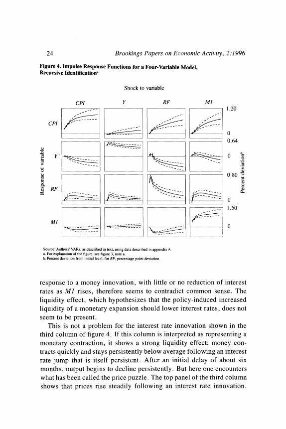
24 Brookings Papers on Economic Activity, 2:1 996
Figure 4. Impulse Response Functions for a Four-Variable Model, Recursive Identificationa
Shock to variable
CPI Y RF Ml 1.20
CPI
0 0.64
0.80
RF/
M1 X - -- == 0 1.50
MI -.~~------- 0
Source: Authors' VARs, as described in text, using data described in appendix A. a. For explanation of the figure, see figure 3, note a. b. Percent deviation from initial level; for RF, percentage point deviation.
response to a money innovation, with little or no reduction of interest rates as Ml rises, therefore seems to contradict common sense. The liquidity effect, which hypothesizes that the policy-induced increased liquidity of a monetary expansion should lower interest rates, does not seem to be present.
This is not a problem for the interest rate innovation shown in the third column of figure 4. If this column is interpreted as representing a monetary contraction, it shows a strong liquidity effect: money con- tracts quickly and stays persistently below average following an interest rate jump that is itself persistent. After an initial delay of about six months, output begins to decline persistently. But here one encounters what has been called the price puzzle. The top panel of the third column shows that prices rise steadily following an interest rate innovation.
Eric M. Leeper, Christopher A. Sims, and Tao Zha 25
Interpreting the third column as a monetary contraction therefore re- quires accepting that monetary contraction produces inflation, which seems as unlikely as the notion that monetary expansion does not lower interest rates.
The fourth column, if it is the monetary policy shock, displays a liquidity puzzle. However, this and the price puzzle of the third column might be eliminated by taking something close to a difference of the two columns. The third column less the fourth would show a positive movement in the funds rate that is less persistent than that in the third column, a negative movement in MI that is more pronounced than in either column individually, a negative movement in Y with less of an initial positive blip as in the third column but with less persistence, and little movement in CPI. In fact, a set of restrictions on A, that in itself has some appeal delivers approximately this result. We present this very small model not as a preferred interpretation of the data, but as an illustration of types of reasoning and interpretation that we apply in more complicated settings, below.
Suppose that, because data on the price level and output emerge only after complex and time-consuming collection and processing, monetary policymakers do not respond within the month to changes in CPI and Y. Suppose, further, that CPI and Y are not responsive within the month to changes in RF and MI. The justification for this assumption is that there are planning processes involved in changing output and in chang- ing the prices of final goods. This is not to say that CPI and Y show no short-run changes. Crop failures, new inventions, consumer dissatis- faction with the new fall line of coats can all result in such short-run variation. But the financial signals embodied in monetary variables are postulated to influence CPI and Y smoothly over time, and very little within a month. This set of restrictions can be displayed in a matrix of Xs and blanks as follows:
Sector Variable CPI Y RF Ml
P CPI X X P Y X X I RF X X X X F Ml X X
The Xs indicate coefficients in A, that are unrestricted, and the blanks indicate coefficients that are postulated to be zero. The first row gives the names of the variables, and the first column gives the names of the

26 Brookings Papers on Economic Activity, 2:1996
sectors in which disturbances or shocks originate. The F shock repre- sents random variation in Federal Reserve behavior, the two P shocks represent the behavior of private sector variables that do not respond quickly to financial signals, and the I shock represents other disturb- ances to private sector behavior ("I" stands for information, meaning that this component of nonpolicy behavior responds quickly to new information).22 The two P equations have the same restrictions and are therefore indistinguishable. They can be premultiplied by any ortho- normal (2 x 2) matrix and yet satisfy the same restrictions. Since these two equations do not have separate interpretations, we normalize them arbitrarily by changing the Y coefficient in the first row from an X to a blank. This results in a system that is overidentified by one restriction. The results of estimating this system are displayed in figure 5.
The fourth column of figure 5 is a plausible candidate for a measure of the effect of tightening monetary policy. RF rises initially, but re- turns to its original level over the course of about a year. MI declines, and most of the variation in MI is accounted for by these policy dis- turbances. Y declines persistently, but not much of the overall variance in output is attributed to the policy disturbance. CPI moves negligibly- very slightly downward. There are some problems with the interpreta- tion. Since the output decline is so small (only about a tenth of a percent), the price decline is negligible, and the interest rate increase is so temporary, it is hard to understand why MI responds so strongly and persistently (almost a full percentage point).
The first three columns show that every private sector shock that implies inflation elicits a contractionary response from the interest rate. As we observe above, in discussing the robustness of conclusions from identified VARs, this means that certain aspects of the results are not sensitive to the identifying assumptions. Most of observed variation in the interest rate is accounted for by these endogenous responses, not by what have been identified as policy shocks. Most of the variation in output and prices is accounted for by the first and third columns, which
22. We could have labeled this equation MD-for money demand-as it contains contemporaneously all four of the traditional arguments of liquidity preference in an ISLM model. However, over much of our sample period, most of the deposits that make up MI paid interest, so a short interest rate such as RF did not represent the opportunity cost of holding MI. Probably more important, in this small model this sector has to be the locus of all nonpolicy effects on the interest rate and MI. Therefore we would not insist that this equation be interpreted as money demand.

Eric M. Leeper, Christopher A. Sims, and Tao Zha 27
Figure 5. Impulse Response Functions for a Four-Variable Model, Nonrecursive Identificationa
Shock to sector P P I F
1.20
CPI IA t;XO
0.75
0.70
,, RF - I =9==_=
Ml'---- - - - ------=t 0.75
ml
Source: Authors' VARs, as described in text, using data described in appendix A. a. For explanation of the figure, see figure 3, note a. b. Percent deviation from initial level; for RF, percentage point deviation.
look like supply shocks, in that they move prices and output in opposite directions. The response of interest rates to the inflationary shock is at least as strong in these cases as when output moves in the same direction as prices, as in the second column. From figures 4 and 5, it appears that there is no possibility of transforming the system to produce a column in which interest rate increases are followed by substantial price declines. It might be possible, by approximately differencing the second and third columns of figure 5, to produce another pattern similar to that in the fourth but with stronger output effects and weaker effects on M1.
Although this model is simple, the basic approach-excluding cer- tain variables from a contemporaneous impact on policy behavior, while asserting that certain private sector variables respond only with a delay to financial variables-has been followed in one form or another in the

28 Brookings Papers on Economic Activity, 2:1996
identified VAR literature since Sims's work in the mid- 1980s, at least.23 Nonetheless, this model cannot be a stopping place in our analysis. Analysts use an array of additional variables-for example, stock prices, long interest rates, exchange rates, commodity price indexes- to forecast prices and output, and Federal Reserve behavior could cer- tainly depend on such indicators of the state of the economy. By omit- ting such variables, we relegate their effects to the disturbance term.
Reserves
Ml responds quickly to private sector behavior and is not directly controlled in the short run by the Federal Reserve. This suggests that one should expect problems in interpreting MI suprises as disturbances to monetary policy. One way to circumvent the fact that much of the variation in MI is demand determined is simply to replace Ml with a reserve aggregate that the Federal Reserve arguably might control more directly. Textbook discussions of the money multiplier might lead one to think that this would not qualitatively change the results. But this is not the case. Consider figure 6, which shows what happens when one replaces MI by total reserves adjusted for changes in reserve require- ments (TR) in the model of figure 3.24 The output response to a money shock, already modest in figure 3, has almost completely disappeared, and the price response is also much weaker. It is possible that this result is moving closer to the truth: by using Ml or a measure of M2, one can confuse endogenous components of the monetary aggregate with policy disturbances, thus exaggerating the effects of policy. However, we
23. Sims (1986). 24. We have discovered in the course of our work that "adjustment for changes in
reserve requirements" has dubious effects on the reserve series. Because of the way in which the series is constructed, the ratio of adjusted to unadjusted reserves varies substantially from month to month, even in periods when there is no change in reserve requirements, because of fluctuations in the distribution of deposits across categories with different reserve requirements. This creates a component of demand-determined fluctuations in "reserves" that has nothing to do with the Federal Reserve's actions to change the volume of reserves. In our modeling, we have sometimes found that even the signs of responses of adjusted and unadjusted reserves differed and that unadjusted reserves seemed to have a stronger relation to other nominal variables than adjusted reserves. Unadjusted reserves does show occasional large jumps-when requirements change and the change is accommodated by the Federal Reserve-that do not have the same effects as reserve changes unaccompanied by changes in requirements. This topic deserves further exploration.

Eric M. Leeper, Christopher A. Sims, and Tao Zha 29
Figure 6. Impulse Response Functions for a Three-Variable Model Including Total Reserves, Recursive Identificationa
Shock to variable CPI Y TR
- - - 1.60
CPI '
- 0~~~~~~~~ i5ES_ L X .= 0.75
0 0
- ---- ---- 1.60
TR - - ~~~~~~~~~~~~~~0
Source: Authors' VARs, as described in text, using data described in appendix A. a. For explanation of the figure, see figure 3, note a. b. Percent deviation from initial level.
show below that it is equally possible to maintain that reserves contain a substantial demand-determined component, so that neither surprise changes in reserves nor surprise changes in the money stock are good measures of monetary policy.25
Three studies-by Steven Strongin; Lawrence Christiano, Martin Eichenbaum, and Charles Evans; and Ben Bernanke and Ilian Mihov- introduce some details of the banking system to analyze the conse- quences of the Federal Reserve's allocation of total reserves between borrowed and nonborrowed reserves.26 By concentrating exclusively on
25. Gordon and Leeper (1994) estimate separate models with reserves and with M2 as the monetary aggregate. Their models are larger and use quite different identifying assumptions than ours here, and they obtain quite different results.
26. Strongin (1995); Christiano, Eichenbaum, and Evans (1996); Bernanke and Mihov (1995).

30 Brookings Papers on Economic Activity, 2:1996
the reserves market, thus entirely omitting consumer-level monetary aggregates from the model, this line of work downplays the importance of private sector money demand behavior. These models also tend to assume a recursive economic structure, with sluggish private sector variables appearing first in the recursive ordering. In addition, the au- thors typically do not discuss thoroughly the restrictions on nonpolicy equations that are necessary to justify their interpretations. Bernanke and Mihov address this shortcoming by providing economic interpre- tations for the banking sector equations in Strongin's and in Christiano, Eichenbaum, and Evans's models.27 These interpretations involve re- strictions not imposed by the original authors.
These reserves models can be understood in the context of a six- variable system, including output, the price level, commodity prices (PC), the federal funds rate, nonborrowed reserves (NBR), and total reserves. The work summarized here excludes the discount rate on the grounds that it is an administered rate that does not play an important role in month-to-month policy decisions. The infrequent changes in the discount rate are taken to be mainly delayed responses to already ex- isting information. The following informal table describes the models in terms of their A, matrices:
Sector Variable Y CPI PC RF NBR TR
P Y C P CPI C C I PC c c c F RF c c c x x x B NBR c c c x x x B TR c c c x x x
Equations are grouped into sectors. If a cell is filled, the variable spec- ified on the top row enters that equation; C denotes a coefficient that is nonzero across models, and X denotes a coefficient that may be nonzero in different specifications. Empty cells correspond to zero restrictions. There are four behaviorally distinct sectors in the model: private slug- gish (P), information (I), Federal Reserve policy (F), and the banking system (B). As before, the private sluggish sector describes aspects of private sector behavior that respond slowly to financial variables, while the I sector describes those aspects that respond without delay. Behavior
27. Bernanke and Mihov (1995) also present a simultaneous model in which policy and banking behavior interact to determine equilibrium prices and quantities.
Eric M. Leeper, Christopher A. Sims, and Tao Zha 31
within the private and information sectors is not specified, so shocks associated with those equations have no clear economic meaning other than being disturbances that are not associated with monetary policy or banking behavior.
The six-variable system allows up to twenty-one coefficients to be freely estimated. Since the first three columns take up fifteen coeffi- cients, no more than six unrestricted coefficients in the lower right (3 x 3) matrix may be estimated. Production and information sector variables enter policy and banking sector equations, implying that those sectors observe and respond to output, overall prices, and commodity prices contemporaneously. Variables like commodity prices, which are determined in auction markets, can be continuously observed, so it may be reasonable to assume the Federal Reserve responds to information gleaned from such series. The assumption that the Federal Reserve knows current values of real GDP and consumer prices, however, is at best an approximation to its actual information set.
Bernanke and Mihov reinterpret the work of Strongin and of Chris- tiano, Eichenbaum, and Evans by attaching behavioral meaning to each equation in the F and B sectors. They impose the restriction that the coefficients on TR and NBR in the fifth equation have equal magnitudes but opposite signs, reflecting a view that the demand for borrowed reserves (BWR) should be homogeneous in the overall level of reserves. (There is certainly no reason why this has to be true, especially in the short run, as here, although it may be a reasonable working hypothesis.) The inclusion of Y and CPI in the relation follows from the fact that the demand for reserves is derived from the need to satisfy reserve requirements and the desire to manage reserve positions closely. The presence of PC is more difficult to justify; there are many other varia- bles that could more appropriately be included in the derived demand function.
Strongin does not provide such a complete interpretation of the F and B sectors. He does not impose Bernanke and Mihov's assumption of homogeneity, but he adds the restrictions that demand for TR is interest inelastic in the short run and is unrelated to NBR, and that the Federal Reserve sets the supply of NBR without regard to the current funds rate. Thus the monetary policy shock is a change in the distri- bution of a given quantity of total reserves between borrowed and nonborrowed reserves. This leaves Strongin with an exactly identified
32 Brookings Papers on Economic Activity, 2:1996
model that can be put into recursive form for easy estimation. The following informal table presents his model of reserves market behav- ior, showing his version of the lower right corner of the six-variable model that we have shown above. We should also note that Strongin's original identification does not include PC.
Sector Variable RF NBR TR
F RF X X B NBR X X X B TR X
Strongin justifies the assumption that demand for reserves is interest inelastic by appealing to institutional rigidities. He argues that within a reserve maintenance period, the banking system as a whole must borrow at the discount window to meet a reserve shortfall. Given that the demand for required reserves is largely determined by current and past deposits, if the demand for excess reserves is unresponsive to policy, in the short run the quantity of total reserves will be determined entirely by demand.28 Although persuasive at the high frequencies as- sociated with reserve settlement periods, the argument carries less force at the monthly frequency of Strongin's data. Figure 7 shows the relation of excess reserves to monthly changes in required reserves over our sample period. While there are more reserves relative to the monthly changes early and late in the sample, over the whole period the changes and the excess reserves are of the same order of magnitude. Banks therefore have substantial room to trade the tighter management of reserves against the interest costs of carrying excess reserves. In fact, simple regressions of excess reserves on interest rates suggest a sub- stantial interest elasticity in excess reserves.
The restriction that is most important in distinguishing Strongin's conclusions from those of other researchers is the claim that the Federal Reserve pays no attention within the month to the current federal funds rate. Most observers think, instead, that the Federal Reserve sets target values for the funds rate and undertakes open market operations to stay close to those targets on a time scale considerably shorter than one
28. In terms of the estimated VAR, the entire monthly innovation in total reserves is attributed to shifts in the demand function. A necessary condition for the elasticity restriction is that the demand for excess reserves be completely unresponsive to any variables that policy may affect immediately. For further details, see Strongin (1995, pp. 467-72).
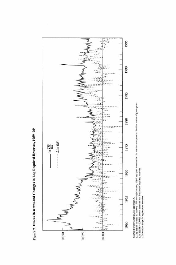
00
00 0
- U~~~~~~~~~~~~~~~~~~~~
rA~~~~0
IL)0
U, ~~~~~~~~~~~~~~~~~~~~~~~~~~~~~~~~~~~~~~~~~~~~~~~~~~~~~~~~~~~~~~~~~~~~~~,
"Cu~~~~~~~~~~~~~~~~~~~~~~~~~~~~~~~~~~~~~~~~~~~~~~~~~~~~~~~~~~~~~~~~~~~~~~'
- U >
U, -~~~~~~~~~~~~~~~~~~~~~~~~~~~~~~~~~a > -
Cu~~~~~~~~~~~~~~~~~~~~~~~~~~~~~~~~~~~~~~~~~~~~~~C CU UU~~~~~~~~~~~~~~~~~~~~~~~~~~~~~~~~~~~~~~~~~~~~~~~~~~~~~~~~~~~~~~~~~~~~~~L
U, -- U0~~~~~~~~~~~~~~~~~~~~~~~~~~~~~~Cs- - U.-~~~~~~~~~~~~~~~~~~c
U, ----~~~~~~~~~~~~~~~~~~~~~~~~~~~~~~~~~~~~~~~~~~~~~~~~~~~~~~~~~~~~~~~~~~~L U,~~~~~~~~~~ 6c
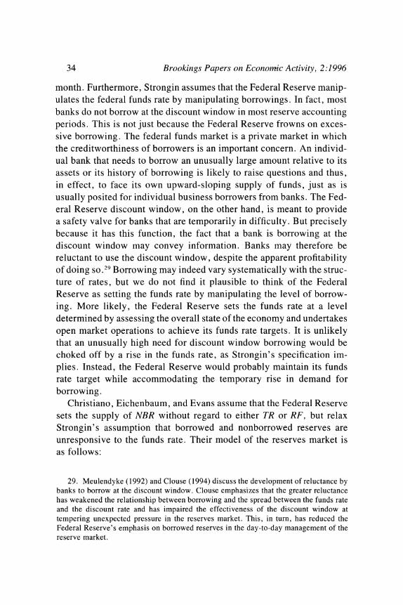
34 Brookings Papers on Economic Activity, 2:1996
month. Furthermore, Strongin assumes that the Federal Reserve manip- ulates the federal funds rate by manipulating borrowings. In fact, most banks do not borrow at the discount window in most reserve accounting periods. This is not just because the Federal Reserve frowns on exces- sive borrowing. The federal funds market is a private market in which the creditworthiness of borrowers is an important concern. An individ- ual bank that needs to borrow an unusually large amount relative to its assets or its history of borrowing is likely to raise questions and thus, in effect, to face its own upward-sloping supply of funds, just as is usually posited for individual business borrowers from banks. The Fed- eral Reserve discount window, on the other hand, is meant to provide a safety valve for banks that are temporarily in difficulty. But precisely because it has this function, the fact that a bank is borrowing at the discount window may convey information. Banks may therefore be reluctant to use the discount window, despite the apparent profitability of doing so.29 Borrowing may indeed vary systematically with the struc- ture of rates, but we do not find it plausible to think of the Federal Reserve as setting the funds rate by manipulating the level of borrow- ing. More likely, the Federal Reserve sets the funds rate at a level determined by assessing the overall state of the economy and undertakes open market operations to achieve its funds rate targets. It is unlikely that an unusually high need for discount window borrowing would be choked off by a rise in the funds rate, as Strongin's specification im- plies. Instead, the Federal Reserve would probably maintain its funds rate target while accommodating the temporary rise in demand for borrowing.
Christiano, Eichenbaum, and Evans assume that the Federal Reserve sets the supply of NBR without regard to either TR or RF, but relax Strongin's assumption that borrowed and nonborrowed reserves are unresponsive to the funds rate. Their model of the reserves market is as follows:
29. Meulendyke (1992) and Clouse (1994) discuss the development of reluctance by banks to borrow at the discount window. Clouse emphasizes that the greater reluctance has weakened the relationship between borrowing and the spread between the funds rate and the discount rate and has impaired the effectiveness of the discount window at tempering unexpected pressure in the reserves market. This, in turn, has reduced the Federal Reserve's emphasis on borrowed reserves in the day-to-day management of the reserve market.

Eric M. Leeper, Christopher A. Sims, and Tao Zha 35
Sector Variable RF NBR TR
F RF X B NBR X X X B TR X X
Their rationale for this identification of policy is that open market operations directly affect nonborrowed reserves, making NBR a control variable for the monetary authority. As discussed above, though, the fact that policy authorities choose a variable does not imply that they choose not to make it respond to other variables. In regard to their assumption that the Federal Reserve pays no attention within the month to the funds rate, our arguments against Strongin's specification apply.
In previous work, Sims notes that a price puzzle-rising interest rates accompanied by inflation-might emerge in a model that does not include a rich enough specification of the information available to pol- icymakers.30 If policymakers can observe variables that forecast infla- tion, but those variables are not included in the model, there will be apparently unpredictable changes in interest rates that are actually sys- tematic responses to information implying that inflation is on the way. This could give the impression that tightening monetary policy gener- ates inflation. Christiano, Eichenbaum, and Evans introduce commod- ity prices to reduce this source of bias: policy authorities are assumed to observe and react to current values of commodity prices. However, these authors merge commodity prices with other variables in the P sector and make them share the sectoral property of no within-month response to monetary policy variables. Since commodity prices are determined in thick auction markets and change daily, this restriction on PC seems strained.3 1
Under Strongin's behavioral assumptions, an expansionary policy shock increases NBR and decreases BWR by exactly the same amount. Because demand for reserves is inelastic, adjustment to a new mix of NBR and BWR for a given quantity of TR must fall entirely to the funds rate. With only the funds rate free to equilibrate supply and demand for NBR, Strongin's policy effects resemble, in exaggerated form, the re-
30. Sims (1992). 31. Gordon and Leeper (1994) impose the similarly dubious assumption that long
interest rates show no within-month response to monetary policy variables, which amounts to assuming away standard term structure connections among interest rates.
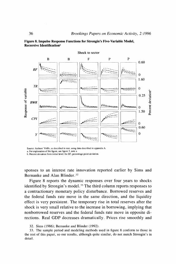
36 Brookings Papers on Economic Activity, 2:1996
Figure 8. Impulse Response Functions for Strongin's Five-Variable Model, Recursive Identification"
Shock to sector
B B F P P 0.60
-------- 1.60- -
TR -- -0
0.25 .
BWR - - -
- ~~~1.50
CPI - - - X n
~0 0.60
Source: Authors' VARs, as described in text, using data described in appendix A. a. For explanation of the figure, see figure 3, note a. b. Percent deviation from initial level; for RF, percentage point deviation.
sponses to an interest rate innovation reported earlier by Sims and Bernanke and Alan Blinder.32
Figure 8 reports the dynamic responses over four years to shocks identified by Strongin's model.33 The third column reports responses to a contractionary monetary policy disturbance. Borrowed reserves and the federal funds rate move in the same direction, and the liquidity effect is very persistent. The temporary rise in total reserves after the shock is very small relative to the increase in borrowing, implying that nonborrowed reserves and the federal funds rate move in opposite di- rections. Real GDP decreases dramatically. Prices rise smoothly and
32. Sims (1986); Bernanke and Blinder (1992). 33. The sample period and modeling methods used in figure 8 conform to those in
the rest of this paper, so our results, although quite similar, do not match Strongin's in detail.
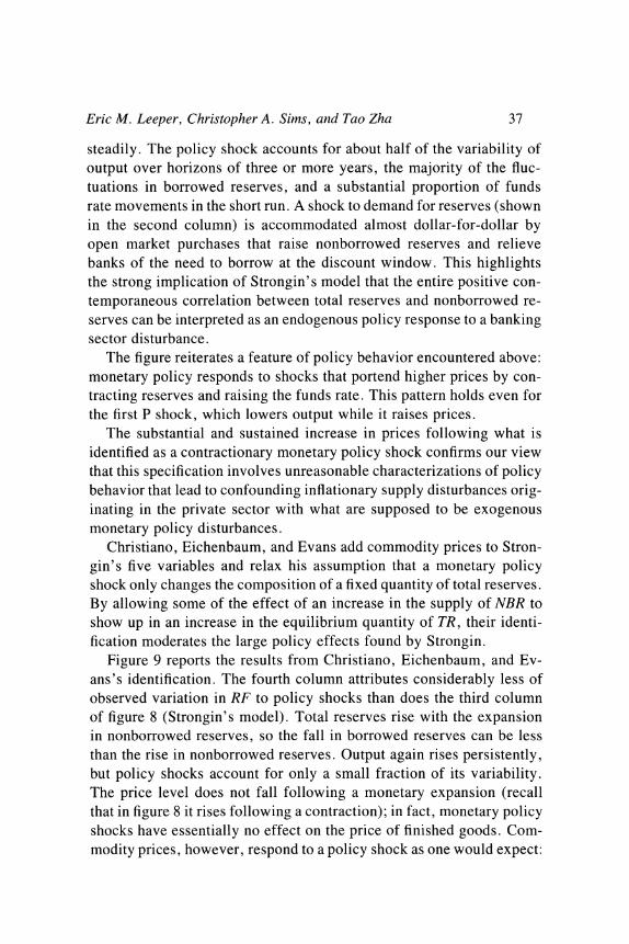
Eric M. Leeper, Christopher A. Sims, and Tao Zha 37
steadily. The policy shock accounts for about half of the variability of output over horizons of three or more years, the majority of the fluc- tuations in borrowed reserves, and a substantial proportion of funds rate movements in the short run. A shock to demand for reserves (shown in the second column) is accommodated almost dollar-for-dollar by open market purchases that raise nonborrowed reserves and relieve banks of the need to borrow at the discount window. This highlights the strong implication of Strongin's model that the entire positive con- temporaneous correlation between total reserves and nonborrowed re- serves can be interpreted as an endogenous policy response to a banking sector disturbance.
The figure reiterates a feature of policy behavior encountered above: monetary policy responds to shocks that portend higher prices by con- tracting reserves and raising the funds rate. This pattern holds even for the first P shock, which lowers output while it raises prices.
The substantial and sustained increase in prices following what is identified as a contractionary monetary policy shock confirms our view that this specification involves unreasonable characterizations of policy behavior that lead to confounding inflationary supply disturbances orig- inating in the private sector with what are supposed to be exogenous monetary policy disturbances.
Christiano, Eichenbaum, and Evans add commodity prices to Stron- gin's five variables and relax his assumption that a monetary policy shock only changes the composition of a fixed quantity of total reserves. By allowing some of the effect of an increase in the supply of NBR to show up in an increase in the equilibrium quantity of TR, their identi- fication moderates the large policy effects found by Strongin.
Figure 9 reports the results from Christiano, Eichenbaum, and Ev- ans's identification. The fourth column attributes considerably less of observed variation in RF to policy shocks than does the third column of figure 8 (Strongin's model). Total reserves rise with the expansion in nonborrowed reserves, so the fall in borrowed reserves can be less than the rise in nonborrowed reserves. Output again rises persistently, but policy shocks account for only a small fraction of its variability. The price level does not fall following a monetary expansion (recall that in figure 8 it rises following a contraction); in fact, monetary policy shocks have essentially no effect on the price of finished goods. Com- modity prices, however, respond to a policy shock as one would expect:

38 Brookings Papers on Economic Activity, 2:1996
Figure 9. Impulse Response Functions for Christiano, Eichenbaum, and Evans's Six-Variable Model, Recursive Identificationa
Shock to sector
p P P F B B -,<3 -< > < f 0.60
1.25
CPI -- --
L ~~~~~~~~~~~~0 .0 PC + ;. l g > > 0 < 4.00
- - -- ~1.60 .
o NBR - X - @ 0
0.80
RF' '- - -
1.50
TR 7 W15 T - ----- --
- - - - - -- -- 0
Source: Authors' VARs, as described in text, using data described in appendix A. a. For explanation of the figure, see figure 3, note a. b. Percent deviation from initial level; for RF, percentage point deviation.
an expansionary shock increases commodity prices as it lowers interest rates.
The response of policy to information about future inflation is as strong here as in the other specifications that we have examined. The third column of figure 9 shows that a jump in commodity prices sig- naling a smoothly increasing price level induces a smooth tightening of reserves and a smooth increase in the funds rate. The endogenous re- sponse of policy to production, information, and banking sector dis- turbances is the dominant source of funds rate variability; policy shocks account for only a small proportion of the error variance in the funds rate .34
34. Christiano, Eichenbaum, and Evans also consider the results of identifying pol- icy with funds rate innovations that are orthogonal to Y, CPI, and PC. The effects are

Eric M. Leeper, Christopher A. Sims, and Tao Zha 39
Christiano, Eichenbaum, and Evans's model produces estimates of the effects of policy disturbances that are, in themselves, believable. However, they are built on assumptions about policy behavior and the reaction of the economy to monetary policy that do not seem plausible.
An Integrated Approach
The research that we survey above treats reserves and MI as mutually exclusive in a model, probably because of the technical and conceptual problems of working with models of more than six or seven variables. In this section we consider two models that include both types of mon- etary aggregate, hoping to gain insight into how bank behavior and Federal Reserve policy interact.
Modeling Federal Reserve and Banking System Behavior
It is appealing to think that by using data on variables directly con- trolled by the Federal Reserve (for example, reserves, the federal funds rate, or the Federal Reserve discount rate), together with others that are of more direct concern to banks (such as bank loans, M2, MI, a bank loan rate index, or a deposit rate index), one might devise restrictions on which variables have an immediate impact on which agent, thereby disentangling the behavior of the banking system from that of the Fed- eral Reserve. However, this enterprise is not so straightforward as separating component sectors of the private economy, or supply and demand in some market. Instead of two collections of individually negligible agents, as in a competitive supply and demand model, in this case there is one such collection (the banks) and a single agent (the Federal Reserve) that is concerned with regulating that collection. Data on most aspects of bank behavior and balance sheets are collected regularly and with little delay by the Federal Reserve, as part of its regulatory function.
We therefore do not aim to model Federal Reserve behavior and
stronger than when NBR innovations are used-as one would expect, they fall midway between the results in figures 8 and 9. This occurs because a positive funds rate inno- vation lowers NBR but raises TR slightly, implying that BWR does not increase dollar for dollar with the decline in NBR.

40 Brookings Papers on Economic Activity, 2:1996
banking system behavior with separate blocks of equations. Rather, we distinguish two aspects of Federal Reserve behavior: macroeconomic policy and bank regulation. The macroeconomic aspect represents the Federal Reserve's responsibility for controlling inflation and attention to its effects on the overall level of economic activity. The regulatory aspect represents the Federal Reserve's concern that the banking system function smoothly and efficiently. In the day-to-day operation of the Federal Reserve open market desk, keeping track of the level of reserves and of deposit flows that generate changes in reserve requirements is a central concern, as is the federal funds rate. Therefore it might seem that any candidate for a Federal Reserve behavior equation should in- clude, at a minimum, a reserve variable and the federal funds rate. But in our view, the Federal Reserve pays attention to reserve and deposit flows in the short run mainly because of their potential impact on the funds rate, for which it sets targets mainly in the light of broader macroeconomic conditions. It tracks shifts in reserve requirements in order to accommodate them and avoid credit market disturbances and unwanted short-run macroeconomic impacts. We aim to define one equation or block of equations that reflects how the Federal Reserve sets the desired level of interest rates in relation to the state of the economy as a whole, and another equation or block of equations rep- resents the combined behavior of the banking sector and the Federal Reserve in relating reserves to deposit flows.
We model the behavior of the Federal Reserve as not depending directly-within the month-on final goods prices, output, or GDP components, on the grounds that these variables can be measured only with substantial delay. In principle, we think it reasonable to allow Federal Reserve behavior to depend within the month on financial mar- ket variables that might serve as indicators of the state of the economy and that are observable on a daily basis-for example, the value of the dollar, a stock price index, long interest rates, or a commodity price index. However, there is an argument for imposing a lag even on the effects of these policy variables. Significant shifts in the Federal Re- serve's macroeconomic policy stance require a time-consuming process of consultation, analysis, and consensus building. We consider speci- fications both with currently observable financial variables included in the Federal Reserve's reaction function contemporaneously and without such variables.

Eric M. Leeper, Christopher A. Sims, and Tao Zha 41
Allowing for a possible response by monetary policy to market in- terest rates raises some difficulties. To understand them, consider a very simple model. Suppose that policy sets a one-period interest rate r(t), responding to an indicator x(t) of the state of the economy, plus a random disturbance E(t). There is a continuously observable two-period interest rate R(t), which is related to r(t) by considerations of term structure. There is also, however, a component of the spread between the two rates, v(t), that may reflect institutional frictions.
Formally, we are supposing
(4) policy: r(t) = ot0x(t) + aox(t - 1) + yR(t) + E(t)
(5) arbitrage: R(t) = -(r(t) + E,[r(t + 1)]) + v(t). 2
To complete the system, the time-series properties of x and v must be specified. Assume that v is serially independent and x is autoregressive, according to
(6) x(t) = Ox(t - 1) + t(t).
Substituting equation 5 into equation 4 gives
(7) r(t) = 2
VLoX(t) + o,x(t- 1) + E(t) + - v(t) + E,r(t + 1). 'Y 2
In order for the system to have a unique solution,
y _
(8) = _ <1,
which is equivalent to y < 1. This points to an inherent drawback in a monetary policy that reacts systematically to market interest rates. Mar- kets depend on policy to fix a path for nominal interest rates. A policy authority that is too sensitive to market rates can create indeterminacy by essentially abandoning its role of anchoring the term structure. In this model, it seems easy to avoid such a situation, since the condition that y < 1 is simple and understandable. But if the policy authority were responding to several rates and to other auctioned market prices that are sensitive to interest rates, it might not be so clear that the boundary of indeterminacy was being crossed.
42 Brookings Papers on Economic Activity, 2:1996
Using equation 6 to solve equation 7 forward leads to
(9) r(t) = 2 ii - ot,i x(t) + x(tf 1)1+
2 E(t) + 4v(t).
One can also substitute equation 9 in equation 5 to produce
i o(I+ 0) + U~(l + 02i) (10) R(t) = - 1o - 04 x()0
+ oIx(t - 1)j + E (t) + + +)v(t).
If all that is known about the policy reaction function is that it has the form of equation 4, there is an identification problem. Any linear trans- formation of the pair of equations 9 and 10 that gives the disturbances in the two equations an identity covariance matrix will result in a system that satisfies the basic restrictions for an identified VAR, but in which both equations have the form of equation 4-a linear equation in r(t), R(t), x(t), and x(t - 1). There will be some versions of the system in which one equation has a scalar multiple of E as a disturbance, but also some versions in which one equation has a scalar multiple of v as the disturbance. If these two equations were part of a larger model, one might allow for other variables to enter the equations, restrict the way in which they enter the two equations, and think, on this basis, that one had identified the two equations. But if, in fact, the other variables were not important, one would have an unidentified, or weakly identi- fied model. One would then run the risk of labeling an arbitrage con- dition as a policy rule and of confusing fluctuations in term risk pre- miums with policy disturbances.
As we have set this model out, it is hard to see why the policy authority should want to react to R. We have assumed that the authority can observe and react to the state of the economy, x, as rapidly as do asset markets. All that the authority accomplishes by reacting to R is to make r depend on the term risk premium, v, in addition to x(t) and x(t - 1). Given that R contains no important information that the policy authority cannot access directly, it seems unlikely that the authority would react to it. Furthermore, even if it did react to R, one would not err greatly by estimating the model as if it did not. If one constrained

Eric M. Leeper, Christopher A. Sims, and Tao Zha 43
the policy reaction function not to contain R, one would emerge with estimates of equation 9 rather than of equation 4. The disturbance term in (9), though, is likely to be almost the same as that in (4). It is reasonable to think that month-to-month variation generated by policy in the short rate is substantially larger than month-to-month variation in the term risk premium.35 Thus, since 4 and y are both less than one, the error term in equation 9 is dominated by variation in E. In other words, even if, by constraining y to zero in equation 4, one mistakenly estimates (9), one will come pretty close to recovering the actual policy disturbance process and thus also to recovering the policy reaction function.
The policy authority would have stronger reason to make y nonzero if it had an information disadvantage; that is, if it was constrained to keep o0 = 0 in equation 4. Then, by reacting to R, the authority could in effect make r(t) sensitive to x(t), despite its inability to observe current x directly. However, in these circumstances, imposing the con- straint that y is equal to zero would firmly identify the system.
This discussion suggests that one should be on the lookout for iden- tification problems when trying to model several interest rates jointly. It makes sense to experiment with identification schemes that allow policy reactions to several longer interest rates and exclude current policy reactions to variables that are observed only with a delay. But such schemes may fail, unable to distinguish between policy equations and arbitrage conditions. In that case, one might obtain good results by allowing current values of a single interest rate in the policy reaction function.
It should be recognized that the criterion for including interest rates in the reaction function is not the degree to which they improve the fit of a least-squares regression. In this simple model, including current R on the right-hand side in a least-squares estimate of a policy reaction function will generally improve the fit and, indeed, will produce an estimate of that linear combination of equation 9 and 10 in which the disturbance is orthogonal to the disturbance in equation 10. If, as is to be expected, v is small, this will be an approximate estimate of the
35. Although this is quite plausible when one considers as the long rate that on a three-month Treasury bill, for example, and as the short rate, that on federal funds, it may be more dubious when one thinks of the long rate as that on a ten-year Treasury bond.
44 Brookings Papers on Economic Activity, 2:1996
arbitrage relationship, almost unrelated to the policy reaction function. Clearly a multivariate approach, with careful attention to simultaneity, is important in order to avoid serious error in this context.36
Through much of our sample period, the behavior of one or more monetary aggregates was a focus of attention. All of our models include at least one monetary aggregate in the Federal Reserve macroeconomic policy equation. A monetary aggregate will also appear in the equations describing the determination of reserves jointly by bank and Federal Reserve behavior, representing the impact of deposit flows on required reserves.
As in our previous specifications of small models, a block that we label P sets "sluggish" private sector variables, which do not respond immediately to financial signals. There is also a block, labeled I, of private sector variables that are set in auction markets and that we allow to depend contemporaneously on everything in the system. Before dis- cussing further issues in model specification, we consider the two sets of exclusion restrictions on AO for which we present estimates below.
We consider one model with thirteen variables and a second, con- taining more banking sector variables, with eighteen variables. Table 1 displays the identification scheme for our smaller model. The varia- bles in the model include both a consumer-level monetary aggregate (MI) and total reserves. We also include CPI, Y, the unemployment rate (U), consumption (C), and both residential and nonresidential in- vestnient (IR and INR, respectively), allowing us to assess the plausi- bility of responses to monetary policy disturbances in some detail. We avoid the complications of having multiple short rates in the same model by including only the three-month Treasury bill rate (R3). In addition, we include four information variables that are observed without delay and might influence Federal Reserve behavior: the Standard and Poor's 500 stock price index (S), the ten-year Treasury bond rate (RIO), a commodity price index (PC), and an index of the value of the dollar
36. Our approach is clearly different from that of most of the empirical reaction function literature (for example, Khoury, 1990) in two respects. One concerns our immediate objectives. We are not primarily interested in explaining or understanding Federal Reserve behavior; we need to model systematic aspects of Federal Reserve behavior in order to estimate accurately how Federal Reserve actions affect the economy. The other is the difference in method that is apparent in this section. Our framework makes it evident that there are identification problems in estimating policy behavior that can be completely thought through only in a multiple equation setting.

ff
6666666
Cu
Cu
Cu 0 z
0
Cu
Cu
Cu Cu-
Cu
>< ><><>< .E
0
Cu
0
0
Cu
Cu
.0 Cu

46 Brookings Papers on Economic Activity, 2:1996
(DOL). The rows and columns of the table correspond to the rows and columns of AO. The Xs indicate coefficients that have been left free. The fractional entries (0.3X throughout this table) indicate coefficients that have been given smaller prior standard deviations than the coeffi- cients corresponding to Xs. These entries can be thought of as soft zero restrictions. We initially estimated the model with the prior covariance matrix determined by the matrix in table 1 (see appendix B for details). However, both in this model and in the larger one that we discuss below, we found that when the soft zero restrictions were used, the shape of the likelihood was highly non-Gaussian, which created numerical dif- ficulties in constructing confidence bands for the impulse responses.37 When we replaced the soft zeros with hard zeros, the non-Gaussian characteristics were greatly diminished, without substantial changes in the estimated impulse responses. Therefore our figures present results for a model with zeros in place of all fractional entries in table 1.
The first two equations in the model, both labeled F/B, combine banking system and Federal Reserve behavior and are normalized by setting the AO coefficient of R3 in the second equation to zero.38 In this specification, the Federal Reserve is modeled as never responding con- temporaneously to variables other than TR or M1. This applies even to available information, such as PC or RIO. The results are almost un- changed if PC is allowed to enter the first two equations contempora- neously. The P block is a standard list of nonfinancial private sector variables, with the addition of M1.
In this model, consumer-level demand for MI is taken to be interest-
37. Since we generate error bands by simulation methods, it may not be clear why a non-Gaussian shape causes us difficulty. We use importance sampling methods, which require that one be able to generate random draws efficiently from a reasonably good approximation to the actual probability density function under examination (for a dis- cussion, see Gelman and others, 1995). With soft zeros, the likelihood has multiple peaks and nonlinear ridges, very non-Gaussian characteristics. Gaussian approximations to this form are so bad that importance sampling is prohibitively inefficient, and we did not have time to program special methods for the particular shapes that we encountered. We should note that, although we have found multiple peaks, these tend either to have qualitatively similar impulse responses or to have much lower likelihood than the ones that we summarize here with impulse responses.
38. In fact, the estimated coefficient on R3 in the second equation is close to zero in any case. Thus the results are almost identical if, instead, the coefficient on TR in the first equation is set to zero, which might be more natural if that equation is to be interpreted as reflecting macroeconomic policy concerns.

Eric M. Leeper, Christopher A. Sims, and Tao Zha 47
insensitive within the month; MI is a private-sector sluggish variable like CPI and Y. We would not defend this specification as necessarily correct; we use it as a working hypothesis. Results are almost com- pletely unchanged if, while excluding PC, one allows R3 to enter all equations of the P block, as would be appropriate if there were a traditional money demand equation in the system-involving R3, MI, CPI, and Y contemporaneously-and if the disturbances in that equation were correlated with other shocks to the P sector. In that case, the triangularizing orthogonalization that we have imposed on the P block would spread R3 coefficients over the whole block, even if the money demand alone contained R3.
The I sector relates the four information variables to all the others, without delay. The P sector is allowed to depend contemporaneously on PC, on the grounds that one aspect of sluggish behavior, price markup rules, might create such a direct dependence.
There are two other variations on this specification that leave results unaffected: allowing U into the F/B block equations, and excluding both PC and R3 from the P block equations. The pattern of responses to the first two shocks is largely unchanged if one replaces total reserves adjusted for reserve requirements (TR) with unadjusted total reserves (TRU). The sixth column does show less tendency for oscillating re- sponses when TRU replaces TR, however. There are also variations that substantially change the pattern of results, which we discuss below, after the results. The results are presented in figure 10.
The first column of figure 10, which, according to the motivation for our scheme of restrictions on AO. ought to reflect disturbances to the macroeconomic policy concerns of the Federal Reserve, shows effects on the economy consonant with its interpretation as a monetary con- traction. Short and long interest rates rise, reserves and MI fall smoothly, output falls and unemployment rises, GDP components fall, commodity prices drop smoothly, and the value of the dollar initially jumps and then continues smoothly upward. Figure 11 shows the first column of figure 10 on a larger scale, with error bands. The error bands are 68 percent probability bands, roughly one standard error on either side of the impulse response. As can be seen, most of the responses are rather sharply estimated. The CPI response, although very small, ap- pears to be more than two standard deviations away from zero in the positive direction for a few months. It does turn negative eventually,
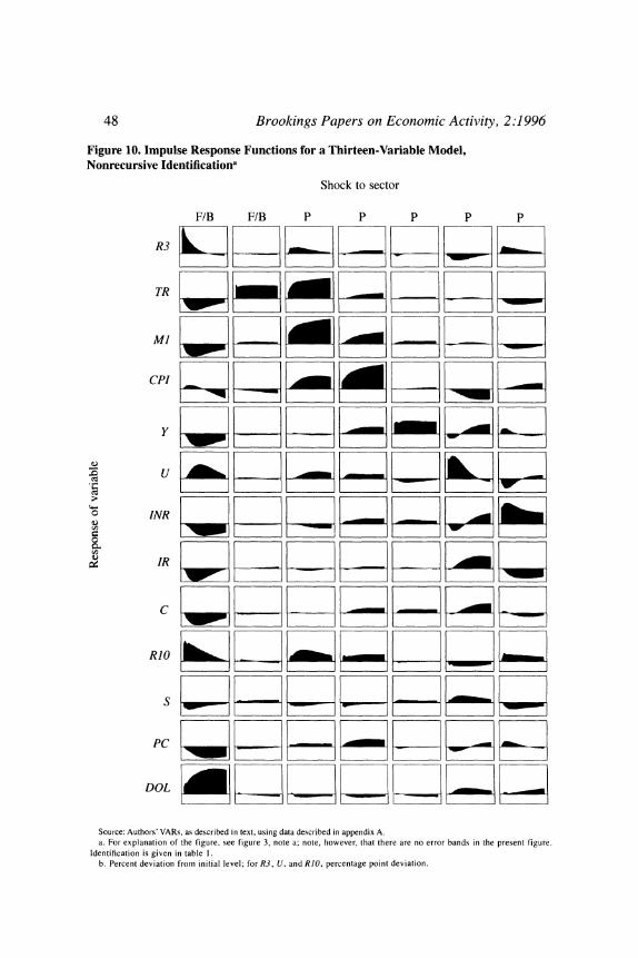
48 Brookings Papers on Economic Activity, 2:1996
Figure 10. Impulse Response Functions for a Thirteen-Variable Model, Nonrecursive Identificationa
Shock to sector
F/B F/B P P P P P
R3A F
TR
Ml -AdNO4
CP' A A+L4
INR
IRI
PC
DOL
Source: Authors' VARs, as described in text, using data described in appendix A. a. For explanation of the figure, see figure 3, note a; note, however, that there are no error bands in the present figure.
Identification is given in table I. b. Percent deviation from initial level; for R3, U, and RIO. percentage point deviation.
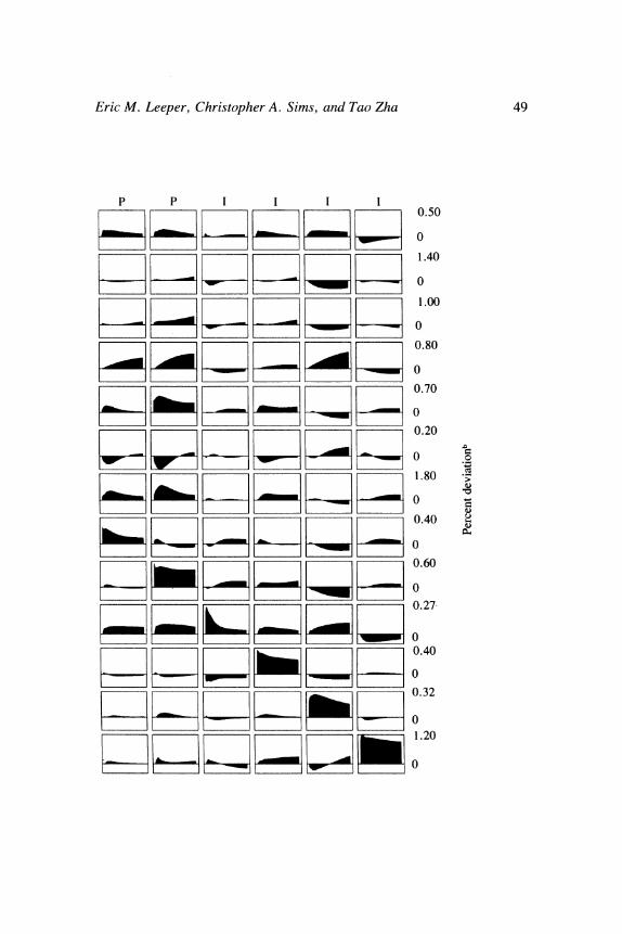
Eric M. Leeper, Christopher A. Sims, and Tao Zha 49
P P I I I I 0.50
1.40
~~~~~~ ~~~~~~~~~~~.0o
9j + 0 ; S ) 0 ; ~~~~~~~~0-80
0.70
0.20
1.80 >
0.40 g
_ 0.60
r 1z 1I 11 1^ Ir 1 0.32
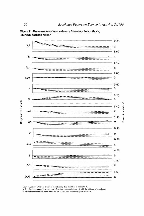
50 Brookings Papers on Economic Activity, 2:1996
Figure 11. Responses to a Contractionary Monetary Policy Shock, Thirteen-Variable Model,
0.54
R 3 -- - - - - - - - - - - - - - - - - - - - 0
1.60
TR-0 TR 5_*,.,-- ----------------------- 1.40
ml 0 Ml - - - - - --- - ---------------------O
1.00
CPI-- 0 O
0.60 Y ~ ~ ~ ~ ~ ~ ~ - -
- - -- -- - ---
- 1 0.20
._ o
1.40
o INR ___E _--------------------- ? 4'
0 2.80
IR -0------- O
0.80
c ~~~~~~~~~~~~~~~0
0.30
RiO ~~~~~~~~~~~~~~~0 4.00
S- 0--- - - -
3.20
PC E------ --0------------------------
- --- . 1.60 D ~ ~~~~-- OL w''}}g''= ------------------------------------ DOL 0
Source: Authors' VARs, as described in text, using data described in appendix A. a. This figure presents a blown-up view of the first column of figure 10, with the addition of error bands. b. Percent deviation from initial level; for R3, U, and RIO, percentage point deviation.

Eric M. Leeper, Christopher A. Sims, and Tao Zha 51
however. The commodity price response is negative at all dates and is roughly two standard deviations away from zero over much of its four- year span.
The second column shows how a model that uses reserves as single monetary aggregate can be treacherous: it appears to reflect the Federal Reserve's accommodation of shifts in demand for reserves that are unrelated to movements in Ml. (This result does not change notably when TRU replaces TR). Perhaps surprisingly, this variation does not consist primarily of variation in excess reserves; required reserves move quite closely in line with total reserves. The variation apparently arises from shifts in the composition of deposits among categories with dif- ferent reserve requirements.
The third column of figure 10 is identified as a private sector shock and moves Ml and TR in the same direction. In this model, we do not try to separate money demand disturbances from other P sector disturb- ances, and this column, because it shows a rise in CPI, does not look like a pure money demand shock. Regardless of its exact nature, it is clear that this disturbance is the most important single source of varia- tion in both Ml and TR and that there is nothing in its estimated form to indicate that the model allocates it to the P sector in error. This is a disturbance that expands the money supply and raises interest rates without affecting output. It seems unlikely that it mistakenly incorpo- rates much of an expansionary monetary policy disturbance. The fact that the model is led by the data to allocate so much variation in monetary aggregates to nonpolicy disturbances shows why use of mon- etary aggregates as one-dimensional policy indicators is unsatisfactory.
In each of the CPI, Y, and U rows of figure 10, the first two columns, corresponding to monetary policy and banking system disturbances, account for only a modest portion of overall variation. For CPI, in fact, the first two columns make a negligible contribution. This model will not admit an interpretation of the sample period as one in which erratic shifts in monetary policy were the prime source of recessions and re- coveries or of episodes of inflation and disinflation.
Across the nonpolicy columns of figure 10, every column in which there is substantial movement in the Treasury bill rate (R3) shows movement in the same direction by CPI and PC. Only in the first monetary policy column do interest rates and either of the price varia- bles show any substantial movement in opposite directions. This sug-

52 Brookings Papers on Economic Activity, 2:1996
gests both that none of the other columns are heavily contaminated with monetary policy shock components and that a large fraction of the variance of interest rates must be attributed to systematic policy re- sponses to the threat of inflation, not to erratic fluctuations in monetary policy. Once again, for the reasons discussed in the section on method, this type of conclusion is robust to variations in the identification scheme.
Table 2 displays the identification scheme for an eighteen-variable model that deletes C and R3 from the thirteen-variable model and adds the Federal Reserve discount rate (RD), the federal funds rate, hourly wage earnings (W), and the following variables related to the banking sector: an index of rates on M2 deposits (RM2), bank holdings of securities (BS), bank loans (BL), and the prime interest rate (RL). As described for the smaller model, we initially estimated with soft zero constraints as shown in the table and obtained reasonable point esti- mates, but encountered numerical difficulties in producing error bands. Once again, converting the soft zeros to hard zeros eliminated the numerical difficulties while leaving the nature of the results largely unchanged. All of our figures therefore present results for the hard zero version of the model.
We display the impulse responses in figure 12. Because two of the interest rates in this model-the federal funds rate and the discount rate-are naturally thought of as set by the Federal Reserve, the first two columns of the figure should be interpreted as responses to policy disturbances. They are similar to the first column of figure 10 in the rows in which the variables are comparable, but in figure 12, the first column apparently represents a short-lived tightening of policy and the second, a longer-lived one. Because the two policy shocks are distin- guished only by an arbitrary normalization, "policy shocks" could take the form of any linear combination of these two columns.
Figure 13 shows the responses to the two columns of policy shocks on a larger scale, with 68 percent error bands. The responses in the first column are fairly sharply determined, although slightly less sharply than the responses in the smaller model. Most of the responses in the second column leave a zero response within the range of high proba- bility, except for interest rates. The disturbance in the first column generates an outflow of Ml deposits, offset initially by a decline in bank securities and, later, by a decline in bank loans. This seems to be

66666 ~ : C) :) 6
X X X X X X X
X X X X X X X X X X X
X X X X X X Ln x X
'c- L X ~~~~X X X X
x x x x X X X X
*Z3 a a aaR R R
C) o6o o66 66
Zu d 0 6666666
Cu XXXX
* Cu XXXXXXXX.
Cu t 66666XXX XXXX
CuRXXXXX.
.CumXXX
Cu XXXX
E m Ds~~~~~~~~~~~~~~~~~~~
VCu X XXXXX,
W0 Xc
Cu g
> C

54 Brookings Papers on Economic Activity, 2:1996
Figure 12. Impulse Response Functions for an Eighteen-Variable Model, Nonrecursive Identificationa
Shock to sector
F F B B B B B P P
RF ;SS 9E RD
RM2
BSE33F33 r E
RL a;;3 -n Ml
INR
IR
CPI
PC
RIO
DOL
Source: Authors' VARs, as described in text, using data described in appendtx A. a. For explanation of the figure, see figure 3. note a, not, however, that there are no error bands in the present figure.
Identification is given in table 2. b. Percent deviation from initial level; for RF, RD, RM2, RL, U, and RIO, percentage point deviation.

Eric M. Leeper, Christopher A. Sims, and Tao Zha 55
P P P P P 1 I 1 I 0.0
0.02
0.90
0.16
0*100
1.20
0.48
0*
sa+eeSHaE3 ?~~~~~~~~~~.7
+SsosaSsO~~~~~~~~~~~~ W;SALW;LESo^7~~~~~~~~~~.6

56 Brookings Papers on Economic Activity, 2:1996
Figure 13. Responses to Two Contractionary Monetary Policy Shocks, Eighteen-Variable Modela
| 0.60 RF - 0
0.32 RD , ,- -- - ------i5=:
BS 0
I 1.80
100
BL 1O 1
RL --- 0. 0 , Ml | -=~-------------- ~~~~~~~~~1 0.8
tt, : ~~------ ---- ---------------------
BSIN j --------------- : 0-~---
Ml ~~~~~~~~~~~~~~~~~0
BL -- --- ----- ----- ? 0.90
CPI~~~zz 1.40= O 0.80 INR - _ --, - -.
0~~~~~~~~~~~~~~~~~~09
C R -- ----I? cP0 1_owe= W 0.90
| | | | l~~~~~~~~~~~~~~.40
0
-R- ------ 400 -.~~~~~~~~~~~~~~09
PC ~~~~~~~~~~~~~~~~~~~.0
RIO ~ ----0.1
D OL. < 1.40 *
_ 0
Source: Authors' VARs, as described in text, using dutu described in uppendix A. u. This figure presents u blown-up view of the first und second columns of figure 12, with the uddition of error bunds. b. Percent deviution from initiul level; for RF, RD, RM2, RL, U, und RIO, percentuge point deviution.

Eric M. Leeper, Christopher A. Sims, and Tao Zha 57
a reasonable pattern for the banking system's response to a monetary contraction and thus reinforces the plausibility of our identification. The fact that RF and RD move with different patterns in the two columns shows that the two variables have considerable independent variation. But there seems to be only one column's worth of substantial non- interest rate effects. A policy action that moved RF and RD in the same direction by about the same amount would have effects that approxi- mately summed across the two columns of figure 13. For the most part, they would be slightly stronger than those shown in the first column of the figure, but not very different overall.
In figure 12, as in figure 10, one column accounts for much of the variance of MI and reserves and shows them moving in the same di- rection and also in the same direction as interest rates. This is the eighth column in figure 12, but the first in the P sector.
Prices and interest rates move in the same direction in response to nearly all disturbances, as they do in the smaller model. In this case, though, there is one disturbance in the I sector (the seventeenth col- umn), in addition to the main policy disturbance, that moves interest rates up and prices down. This disturbance seems to have negligible real effects. It involves a sharp, temporary movement in long rates that seems out of proportion to the small associated movements in RF and RD. Nonetheless, from the form of the responses, this disturbance could possibly be contaminated with a monetary policy shock component.
These results are basically easy to defend, but we would add a note of caution. We are not sure of the implications of the numerical diffi- culties in the less restricted models, which we initially thought more plausible than these. It could be that when we resolve these difficulties we will see that there is much more statistical uncertainty in our results than this presentation would suggest. Also, we have experimented with a version of the larger model that includes the three-month Treasury bill rate in addition to the federal funds rate. This version proves quite capable of producing the kind of identification confusion that we discuss above in the context of our example model, equations 4 and 5. A fitted model that looked reasonable enough might, after some small change in specification or sample period, show impulse response rotation- what looked like a monetary policy shock might emerge as an I sector shock, while the shock formally identified as a monetary policy shock might cease to make sense. This is exactly the pattern that one would
58 Brookings Papers on Economic Activity, 2:1996
expect if the Treasury bill rate were linked to the federal funds rate by term structure arbitrage relationships and contained little informa- tion of use to policy authorities. As we point out above, under such circumstances, inclusion of the Treasury bill rate can weaken identifi- cation without improving the accuracy of the model. We therefore feel justified in responding to these difficulties by considering a model with- out the Treasury bill rate; but it would clearly be more satisfactory to find a way to model the two short rates jointly and maintain robust identification.
Conclusion
This paper is clearly far from the last word on the issues discussed, even in the context of identified VAR research. It remains quite possi- ble, for example, that we are still attributing to policy disturbances some variation that actually originates in adverse supply shocks. This would tend to diminish the estimated price-reducing effects of monetary contraction and exaggerate the estimated output-reducing effects. With similar methods but smaller models, Soyoung Kim finds very small real effects and larger price effects using data for other countries, and David Cushman and Tao Zha, exploiting the identification possibilities that arise for a small open economy, also find small real effects.39
Nonetheless, we believe that our estimates have some chance of being right. Using a larger modeling framework makes possible a clearer understanding of the identification problems and greater confi- dence in interpreting results, since we trace effects across a wider variety of variables. We believe that we establish quite firmly the un- reliability of identifications that treat a monetary aggregate-whether reserves or an M variable-as moving mainly in response to policy disturbances in the short run. The bulk of the movements in both ag- gregates arise from policy accommodating shifts in private sector de- mand. Further, we confirm that most movements in monetary policy instruments are responses to the state of the economy, not random deviations from the usual patterns of behavior of the monetary author- ities. To policy analysts, accustomed to basing policy recommendations
39. Soyoung Kim (1996); Cushman and Zha (forthcoming).

Eric M. Leeper, Christopher A. Sims, and Tao Zha 59
on current and expected economic conditions, this finding is surely not surprising, but it should be disturbing. It implies that close attention to modeling the policy-setting process is essential to accurate statistical assessment of the effects of policy. Much existing empirical policy modeling ignores, or treats casually, the implications of policy endo- geneity. We hope that we demonstrate that careful treatment of policy endogeneity is feasible, as well as important.
APPENDIX A
Data
ALL VARIABLES are monthly time series covering July 1959 through March 1996. Unless otherwise indicated, all calculations described in the text are for the period January 1960 through March 1996, so that the data allow inclusion of a six-period lag. Underlying data for some variables are quarterly; in those cases, we interpolate using the proce- dure described in Chow and Lin (1971). Calculations use natural logs of all variables, except interest rate variables and the variable U. In the figures, however, scales present percentage (or percentage point) de- viations of underlying variables, not log variables.
The following variables use data obtained directly from the Board of Governors of the Federal Reserve System:
BL Total loans and leases at all commercial banks, seasonally adjusted, billions of dollars.
BS Securities at all commercial banks. Computed as total loans and securities less total loans and leases at all commercial banks, seasonally adjusted, billions of dollars.
BWR Borrowed reserves. Calculated by the authors as ln(TRINBR).
Ml MI money stock, seasonally adjusted, billions of dollars.
RD Discount window borrowing rate at the Federal Reserve Bank of New York, percent.

60 Brookings Papers on Economic Activity, 2:1996
RF Federal funds rate (effective rate), percent.
RL Prime rate on short-term business loans. Computed as average of daily figures, percent.
RM2 Deposit-weighted average percent return on M2 deposits.
RR Required reserves, adjusted for breaks due to changes in re- serve requirements, seasonally adjusted, billions of dollars.
R3 Three-month Treasury bill rate, from the secondary market, percent.
RIO Ten-year Treasury bond rate, constant maturity, from the sec- ondary market, percent.
S Standard and Poor's 500 composite stock price index, 1943 =
100.
TR Total reserves, adjusted for breaks due to changes in reserve requirements, seasonally adjusted, billions of dollars.
TRU Total reserves, not adjusted for breaks due to changes in re- serve requirements, seasonally adjusted, billions of dollars.
The following variables use data from other sources:
C Personal consumption expenditures, seasonally adjusted, bil- lions of chain 1992 dollars. Source: Bureau of Economic Anal- ysis, National Income and Product Accounts (NIPA).
CPI Consumer price index for urban consumers (CPI-U), season- ally adjusted index, 1982-84 = 100. Source: Bureau of Labor Statistics (BLS).
DOL Trade-weighted value of the U.S. dollar, index, 1980 = 100. Source: Federal Reserve Bank of Atlanta.
INR Real private nonresidential fixed investment, seasonally ad- justed, billions of chain 1992 dollars. Source: NIPA. Interpo- lated using monthly data on real value of new construction of privately owned nonresidential industrial structures (from the Bureau of Economic Analysis [BEA]); total equipment com- ponent of industrial production, industrial machinery and

Eric M. Leeper, Christopher A. Sims, and Tao Zha 61
equipment component of industrial production, intermediate products and business supplies component of industrial pro- duction (from the Board of Governors of the Federal Reserve System); and manufacturers' shipments to capital goods indus- tries, and manufacturers' shipments of construction materials, supplies, and intermediate products (from the BEA).
IR Real residential fixed investment, seasonally adjusted, billions of chain 1992 dollars. Source: NIPA. Interpolated using monthly data on housing starts, manufacturers' shipments of construction materials, supplies, intermediate products, and real value of new construction of privately owned residential buildings (from the BEA); and construction supplies compo- nent of industrial production (from the Board of Governors of the Federal Reserve System).
PC International Monetary Fund's index of world commodity prices. Source: International Financial Statistics.
PCM Crude materials component of the producer price index, sea- sonally adjusted index, 1982 = 100. Source: BLS.
U Civilian unemployment rate, seasonally adjusted, percent. Source: BLS.
W Wage earnings, seasonally adjusted, dollars per hour. Source: data from 1964 onward are from the Bureau of Labor Statistics, Employment and Earnings. Pre-1964 data are based on our regressions, using actual manufacturing data for 1959-63 as explanatory variables.
Y Real GDP, seasonally adjusted, billions of chain 1992 dollars. Source: NIPA. Interpolated using monthly data on total indus- trial production (from the Board of Governors of the Federal Reserve System), civilian employment for age sixteen years or older (from the Bureau of Labor Statistics, Employment Situ- tation), retail sales (from the BEA) deflated by consumer prices, real personal consumption expenditures (from NIPA), and the National Association of Purchasing Managers' Com- posite Index.

62 Brookings Papers on Economic Activity, 2.1996
APPENDIX B
The Prior
THIS APPENDIX outlines our approach. For sufficient detail on the prior to actually use our methods, and for an appreciation of the numerical and mathematical considerations that lead us to this particular form, see Sims and Zha (1996).
We postulate a joint normal prior, initially with a diagonal covariance matrix, on the elements of AO that are not constrained to zero. In the case of reduced form models, we choose an ordering of the variables that constrains AO to be triangular, an exactly identified normalization. We then specify a joint normal prior on all the coefficients in A, s > 0, conditional on AO. To make the prior center on specifications in which reduced form models for individual variables are random walks, we make the conditional mean of Al IAO be AO itself, while the condi- tional mean of AsIAo, s > 1 is zero. The prior standard deviations of the elements of the AS matrices shrink as s increases, and these elements are initially taken as uncorrelated. It may seem that this approach- constructing the prior from a marginal on AO and a conditional distri- bution for AsIA0, s > 1-is roundabout and complicated, but it turns out to be critical to making the method numerically feasible in large models.
On this base prior we layer additional components, constructed as dummy observations. The dummy observations induce correlations across elements of A in the prior. The dummy observations express the belief that no-change forecasts of the model's variables are likely to be quite good. Of special note is that in large dynamic systems like this, the phenomenon that produces the well-known bias toward stationarity in least-squares estimators produces a bias toward deterministic com- ponents of the model explaining implausibly large fractions of the his- torically observed variation in the data. We find that this type of dummy observation also expresses the belief that models that explain too much with deterministic components are implausible. It appears that using such dummy observations is essential in order to obtain sensible results in models of this scale, yet conventional time-series diagnostic testing might not reveal this bias at work (this point is discussed further in Sims and Zha, 1996).

Eric M. Leeper, Christopher A. Sims, and Tao Zha 63
Although these priors may seem complicated, they are not influential on the character of the results. In small models, in which the bias toward excessively strong deterministic components is not great, a flat prior and our prior produce quite similar results. Our prior tends to make the estimated impulse responses smoother, without changing their overall form. We do not manipulate the prior to make results look more rea- sonable, except in the case of the soft zero constraints in the prior on A, as discussed in the text.

Comments and Discussion
Robert E. Hall: This is roughly the fifteenth anniversary of Sims's original promulgation of the vector autoregression as a tool for macro- economic research. ' For a while, it seemed that the VAR was mainly a vehicle for unproductive data mining. Little attention was paid to iden- tification-arbitrary triangular restrictions were assumed. One heard a lot of stories, not much science. But Sims himself was never a story- teller. In its second decade, the VAR came into its own as a research tool. Careful attention to identification, based on reasonable economic theory, has become the standard. In addition to Sims himself, the lead- ers in this area have been Olivier Blanchard, Mark Watson, and Ben Bernanke.
This paper, with Leeper and Zha, is a comprehensive review of the evidence on the role of monetary policy in the identified VAR frame- work. The two questions considered in the paper are: How large is the spontaneous random element of monetary policy? And how much of the movement of real GDP can be attributed to the spontaneous com- ponent?
Let me say something about the econometric framework used in the paper. The basic statistical model is
y = CE,
where y is a vector of observed innovations in key macroeconomic variables; E is a vector of underlying fundamental driving forces, in-
1. Sims (1980b).
64
Eric M. Leeper, Christopher A. Sims, and Tao Zha 65
cluding the spontaneous elements of monetary policy; and C is a matrix showing the dependence of the variables on the driving forces.
Another way to write this class of models is
Ay= E,
where A is C', the matrix of the structural relations among the varia- bles. Suppose that A (or, equivalently, C) is known-that is, suppose that theory tells one how each driving force affects each observed macroeconomic variable. The covariance matrix of the innovations, fQ = V(y), can be directly observed. It is left to infer the covariance matrix of the underlying driving forces, E V(E). This can be re- covered directly from
A'V(y)A = A'fQA =
Also, one can recover the values of the driving forces from
E = Ay.
Note that the covariance matrix E has N(N - 1)/2 distinct off- diagonals. One can calculate, rather than assume, this many elements of A, if one assumes that these covariances are zero. As the authors mention, this assumption is standard in the VAR approach, whereas it is not generally made within the traditional simultaneous equations framework.
If one takes the hard line that one knows all of the structural coeffi- cients, in either the C sense or the A sense, then one can answer the two questions immediately: one can calculate the driving forces, in- cluding random money, and calculate the part of the movements of real GDP that are attributable to that component (and to each of the other components).
Note that when one considers C or A known, one does not impose the restriction that the driving forces be uncorrelated with each other. When one calculates the covariance matrix of the driving forces, it will have nonzero off-diagonal elements. This is where the computational effort and econometric excitement come in. One can use the assumption that the N(N - 1)/2 distinct off-diagonal elements of the covariance matrix are zero in order to determine the values of that many of the coefficients of C or A. That leaves one with the need to use prior

66 Brookings Papers on Economic Activity, 2:1996
knowledge, derived from theory, to determine the remaining elements of C or A.
The natural framework for handling prior information is that of Baye- sian statistics. This paper is a pioneering effort to apply Bayesian think- ing to the VAR framework. It does so in two ways. First, it imposes mildly held beliefs that the coefficients in the C or A matrices are not too large, and that the most likely forecast is that the current values of the variables will be the same as the lagged values. This procedure tames the tendency for VARs with many variables to overfit the data and have implausible dynamics.
Second, following my suggestion at the Brookings Panel meeting, the authors experiment with prior restrictions on the A matrix that are less than fully dogmatic. These soft zero restrictions result in intractable numerical problems, however. For the moment, it is necessary to be completely dogmatic about the crucial restrictions that identify the model and make it possible to give names to the shocks. Either one knows for sure that a coefficient has a particular value, usually zero, or one does not have a clue.
The paper's econometric framework is well suited to dealing with the authors' basic questions. The coefficient matrices, A or C, tell what part of an observed monetary variable (an element of y, such as Ml, reserves, or interest rates) is induced by other forces (other components of e) and what is the result of the spontaneous component. There are some hints that it would be interesting to look at upper bounds on the size and importance of the spontaneous element. Although this idea is not really formulated or pursued in the paper, I think it should be.
The spontaneous element of a monetary variable cannot be larger, one might suppose, than the innovation in that variable. A model with only zeroes in the row of C that corresponds to the monetary variable, except for the element corresponding to the spontaneous element of monetary policy, provides a bound on the size of the spontaneous ele- ment of monetary policy. This is exactly what the models of figures 3, 4, and 6 do-the triangular models. They show that even if the mone- tary variable is taken as either MI or total reserves and its innovation is taken to be completely spontaneous, the random element nonetheless has little role in the movement of real GDP.
If the point of the paper were only to show that the spontaneous element of monetary policy has little effect on real output, it could end
Eric M. Leeper, Christopher A. Sims, and Tao Zha 67
here. All the rest of the paper works on removing from monetary policy variables the portion that is induced by current developments in the economy. That is unnecessary for the main thesis.
The first attempt to deal with the induced element of the monetary variables relies on the restrictions in the first informal table, with results given in figure 5. There is a problem here, and in all seriously identified VARs, whose solution escapes me. The restrictions in this table are stated in terms of the A matrix, which shows how the observed variables interact with one another. The basic question, and much of the discus- sion, relate to its inverse, the C matrix. The zero restrictions in the table map into complicated restrictions on C. The problem shows up in the first column, where the names of the E impulses are listed alongside those of the variables: the names of variables and impulses are carefully distinguished. What one would like to know, but cannot completely figure out from the table, are the restrictions on the way each impulse enters each observed variable.
The authors' restrictions, asserted with dogmatic certainty, are hardly compelling. Those on the upper right say that neither money nor interest rates affect output or prices in the same month. They do not claim that the immediate effect is small, but that it is strictly zero. Those on the lower left say that there is no response induced in money by output or price developments in the same month. I agree that the within-month effects of money and interest on output and prices are probably fairly small, but that does not make them literally zero. And I have an even stronger suspicion that the Fed gets some inkling about output and prices within the month and responds to that inkling.
Again, the identification comes from the certain knowledge that these four restrictions are true. It must not be interpreted as a belief that the effects are small, because "small" would have to be judged in relation to other effects whose magnitude cannot be known without the restric- tions. This underscores the potential value of a full Bayesian treatment of the prior information.
It would appear that the authors arrived at these restrictions through informal Bayesianism. With respect to figure 5, they find the results plausible because the F column mirrors what they think a monetary policy variable ought to do to the four key macroeconomic variables. This model probably overstates the spontaneous element of monetary policy by ruling out changes induced by output or prices, so that it

68 Brookings Papers on Economic Activity, 2:1996
shares the upper-bound character of the triangular results. Thus it is significant that the model finds almost no role for the spontaneous element of monetary policy in the determination of output.
The next part of the paper discusses earlier work based on strong restrictions-shown in the second informal table-that bar immediate effects of monetary policy on output or prices but do consider feedback from those variables to monetary policy. This work is concerned mainly with untangling monetary instruments and does not pay much attention to the effect of spontaneous monetary policy on output. I think it is fair to say that almost everything that one could learn on that issue could be learned from the simple triangular model suggested by this table, if there were just a single monetary indicator. In effect, one would regress the indicator on all the other contemporaneous innovations and treat the residual as the spontaneous element of monetary policy.
The remainder of the paper looks at quite large models in pretty much the framework of the restrictions of the first informal table. These restrictions differ greatly from those in the existing literature, because they exclude monetary policy responses induced by output and prices. I am skeptical of the payoff from such complexity. Given the shaky basis for identification-that the Fed does not get even the smallest hint about what is currently going on in the economy-what does one gain by putting in so many indicators? The statement in the conclusion that one can be more confident about the truth of this fundamental hypothesis with more variables does not grab me.
Nonetheless, I think the substance of the conclusion is absolutely right: the spontaneous element of monetary policy is small, and it is not a major determinant of movements of real GDP. The paper seems somewhat out of touch with the history of its sample period. Those who believe that monetary policy is an important independent driving force point to episodes in the 1960s and early 1970s. There was, after all, a watershed in monetary policy in 1979, when Paul Volcker took over at the Federal Reserve. And I have not heard anybody call the Greenspan Fed a random, independent contributor to fluctuations. At the same time, the residuals from a Taylor rule in 1972-73 under Arthur Burns are huge. One of the interesting features of the Bayesian approach taken in this paper is that it makes it practical to study separate VARs for different subperiods.

Eric M. Leeper, Christopher A. Sims, and Tao Zha 69
Ben S. Bernanke: This is a brilliant paper that repays close study. Using vector autoregression methods an order of magnitude more so- phisticated than those introduced into economics by Sims in his famous 1980 paper-but similar in spirit-Leeper, Sims, and Zha extract from the aggregate time-series data a surprisingly large amount of informa- tion about the effects on the economy of innovations in monetary pol- icy.' The only broad objection that one might consider making to this work is that in its sophistication it has departed from the appealing simplicity of the original VAR studies and moved closer to the complex econometric models that were the subject of Sims's original critique. This objection would be largely unfair, however. First, the simple fact is that reality is complicated, and a useful econometric methodology must be able to accommodate that fact. Second, relative to traditional simultaneous equation econometric models, the authors' methodology makes more exhaustive use of the dynamic relationships in the data and does so in the context of a full-system, rather than an equation-by- equation, estimation technique.
The paper builds on and synthesizes what has become a fairly large VAR literature on the effects of monetary policy. A key insight of this literature is that the traditional monetarist approach of regressing changes in a macroeconomic variable (such as output) on changes in a lagged monetary policy measure (such as MI growth) cannot identify the effects of monetary policy. The problem is that policy is not exog- enous, but responds to the state of the economy. Hence, for example, the finding that cnanges in output follow changes in the money supply cannot distinguish between the hypotheses that, on the one hand, money supply changes cause changes in output, and on the other hand, both changes in the money supply and subsequent changes in output are caused by some third factor.
The response of the VAR literature to this identification problem has been to focus on the effects of innovations-that is, random, unanti- cipated changes-in monetary policy. If policy innovations are properly identified, the inference that subsequent changes in the economy are caused by the policy changes is valid. In practice, however, the VAR- based approach has difficulties of its own. First, the identified policy
1. Sims (1980b).

70 Brookings Papers on Economic Activity, 2:1996
innovations must be truly exogenous with respect to the state of the economy-arising, for example, from exogenous changes in policy preferences, technical errors in implementing policy, or noisy contem- poraneous data-not reflections of the Federal Reserve's information about current or future economic developments. If what is identified as a policy innovation is, in fact, a reaction by the Fed to information about the economy, not known or accounted for by the econometrician, then incorrect inferences will be drawn about the effect of policy. This problem presumably underlies the liquidity puzzle and price puzzle phenomena discussed both in the earlier literature and in this paper. The second problem is that, as in the earlier monetarist literature, the results depend on an appropriate choice of policy indicator-that is, the indicator must be such that its innovations are due to policy changes, not to some other factor. If, for example, MI is chosen as the policy indicator, but most statistical innovations in MI arise from changes in money demand rather than innovations in monetary policy, then the VAR-based approach will again yield the wrong inferences.
The technical advance that allows the present paper to address both of these problems is the use of Bayesian methods to save degrees of freedom in estimation, which, in turn, permits the estimation of much larger systems. These larger systems can include a longer list of infor- mation variables, such as asset prices; to the extent that the broader set of variables approximately spans the information set used by the Fed to make policy decisions, the first type of bias noted above is mitigated. Larger systems also permit the inclusion of a more complete set of potential policy indicators (such as interest rates, reserve measures, and monetary aggregates), as well as more indicators of economic activity (such as residential construction), which makes it possible to compare a variety of alternative identifications of policy in the same system. The analysis of the robustness of earlier VAR-based results in the context of larger, more complete systems is the major contribution of the paper.
Much of the paper is devoted to discussion of methodological issues and to the alternative models and identifications that the authors have tried. Because of its focus on methodology, it has relatively little to say on how monetary policy works (that is, channels of transmission) or on how it should be used. The substantive conclusions that I took away are (1) that effects of monetary policy on the economy can be robustly identified and are "plausible," in the sense of conforming
Eric M. Leeper, Christopher A. Sims, and Tao Zha 71
qualitatively to conventional wisdom; (2) that interest rates, such as the federal funds rate or the Treasury bill rate, are better indicators of monetary policy than are reserves or monetary aggregates; (3) that over the past thirty-five years monetary policy innovations have made a relatively small contribution to the overall variances of output and prices in the U.S. economy; and (4) that monetary policy responds strongly to the economy-that is, there is a large endogenous compo- nent to policy. I do not necessarily disagree with any of these, but I have a few comments on conclusions 2 and 3, as well as a few related remarks about the econometrics.
In regard to conclusion 2, it should be said that the superiority of interest rate indicators of policy comes as no surprise when one consid- ers how central banks actually operate, not only in the United States but in virtually all developed countries. Currently, almost all central banks smooth overnight (or other very short-term) interest rates, mov- ing their interest rate targets only when deliberately changing their policy stances. This focus on interest rates in the short and medium runs implies that, since changes in the demand for money or reserves are almost entirely accommodated by the central bank, innovations in money or reserves typically mostly reflect demand shocks rather than policy changes. These observations lead to two criticisms of the paper. First, since operating procedures provide an important clue to the choice of the correct policy indicator, why did the authors not explicitly use more information on operating procedures in the identification of the model? In my work with Blinder and, particularly, with Mihov, cited by the authors, I have found that explicit estimation of Fed operating procedures provides a useful way of identifying the policy indicator without having to rely as much as the present paper does on the "rea- sonableness" of impulse response functions as a criterion.2 Indeed, in critiquing the work of some earlier authors, Leeper, Sims, and Zha make informal arguments on the basis of what is known about operating procedures and the institutional structure of the market for bank re- serves; more of this type of reasoning could have been incorporated into the estimation.
Further, when one recognizes that the optimal policy indicator de- pends on the operating procedure and the institutional structure, one is
2. Bernanke and Blinder (1992); Bernanke and Mihov (1995).

72 Brookings Papers on Economic Activity, 2:1996
also forced to admit that the best policy indicator may change over time. For example, Mihov and I find-in line with conventional wis- dom-that during 1979-82, the Fed targeted nonborrowed reserves to a much greater extent than before or since. Therefore it would not be appropriate to use the federal funds rate as a policy indicator for that period. Similarly, it is often argued that the Fed did not adopt funds rate targeting until the latter half of the 1960s. Other countries, such as Germany and Japan, have experienced even more sweeping changes in operating procedure and institutions over the past few decades. The authors' approach ignores the possibility of such changes by assuming an invariant model-in this application, for the entire period 1959-96. This is a shortcoming, but one that might be overcome, for example, by allowing for breaks in some subset of the model's parameters.
With respect to conclusion 3, my inclination is to ask, first, is it true that monetary policy shocks have been unimportant in the postwar period? And second, if it is true, so what? One reason why I am not sure that it is true is precisely the large number of variables included in these systems; while it is hard to judge the number of degrees of free- dom in a Bayesian setup, overfitting-and hence an artificially small estimate of the policy residuals-seems to be a possibility. Also, is the one-month-ahead forecast error the right choice of focus in judging the variance of policy shocks? It may be, for example, that a forecast error of longer horizon is the relevant one for product and labor markets, where nominal contracts (both implicit and explicit) might well last for more than a month.
And even if one agrees that monetary policy shocks explain a small portion of the variance in output and prices over the past thirty years, this is only one of several interesting questions that might be asked about postwar U.S. monetary policy. First, the within-sample variance decompositions say nothing about the potential real effects of monetary policy-which experiences like the Great Depression and the Volcker disinflation suggest are large. To use a perhaps strained analogy, nu- clear explosions account for approximately 0 percent of output variation in the U.S. economy over the past thirty years, but that fact is not informative about what would happen if nuclear weapons were actually used. To assess the potential of monetary policy to move output, one should focus on impulse response functions rather than variance decom- positions (and perhaps consider the effects of "large" rather than "typ-

Eric M. Leeper, Christopher A. Sims, and Tao Zha 73
ical" innovations in monetary policy). Second, the result that monetary policy shocks have played a small role in output variation does not prove that policy was conducted well during the sample period (al- though a small degree of unpredictability is a feature of good monetary policy). In particular, as is well known, this exercise says nothing about the effects of anticipated monetary policy-or, equivalently, of the monetary policy rule-on the economy. Figuring out how to analyze policy rules in a framework of this sort remains an important unsolved problem.
Let me finish where I began, however-with praise. This excellent paper strengthens my belief that identified VAR methods are currently the best available means of measuring the effects of monetary policy changes on the economy. Explaining the detailed dynamic patterns found here and in related work should be a major objective of modern macroeconomic theory.
General discussion: N. Gregory Mankiw noted that there are two strands of literature examining the behavior of the Federal Reserve: one involves estimating policy reaction functions, of which identified VARs are an example; the other, started by David and Christina Romer, looks directly at minutes of the Fed's Open Market Committee to identify spontaneous shifts in monetary policy. To a large extent, these two strands have ignored each others' existence. Romer and Romer's paper suggests that every recession has been preceded by a shift in policy, while the VARs suggest that exogenous monetary policy changes ex- plain only a small portion of economic fluctuations. Mankiw wondered how these two views could be reconciled. Sims noted that the Romers' dummy is not constructed by looking for exogenous random changes in policy, but rather for times at which inflation is explicitly raised as a concern in the Fed's meeting. This makes it a strong candidate for endogeneity. Leeper noted that a study by Matthew Shapiro in fact indicates the Romers' dummy for policy shifts is endogenous. He sug- gested that if their dummy were used in a small VAR system in place of other measures on monetary policy, it would almost surely imply a price puzzle. If it were used in a larger model, such as those in the paper, it would be insignificant.
James Duesenberry welcomed the paper's contribution, noting that although the profession has long recognized the difficulty of estimating

74 Brookings Papers on Economic Activity, 2:1996
the effects of exogenous policy actions, given that much of policy is endogenous, satisfactory answers are still far away. He suggested that the authors' approach might benefit from making use of the information actually available to the Open Market Committee when it meets. One example is the time series constructed by Steve McNeiss of the Federal Reserve Bank of Boston, which draws on the Fed's Green Books that are used in making staff forecasts of unemployment and inflation at the time of the meetings. Such data might allow a better identification of which macroeconomic variables enter the Fed's reaction function.
Several panelists discussed the paper's heavy emphasis on identifi- cation of the innovations and its relative inattention to the economic structure. Duesenberry worried that these new models paid even less attention to the logic of a priori restrictions than the old-fashioned macroeconometric models. He noted that any research needs to start from assumptions and priors, but such information is likely to be as valuable in specifying the economic structure of the model as in re- stricting the innovation errors. Mankiw found it ironic that Sims, who had developed the VAR methodology to diminish the extent to which macroeconomic models rely on a tremendous number of what he had called incredible identifying assumptions on the structure, has, with his coauthors, had to return to making many similar assumptions in order to identify policy effects.
Benjamin Friedman expressed reservations about prospects for dis- covering the effects of the systematic component of monetary policy through the lens of nonsystematic variability. The problems in this approach are readily illustrated by the authors' own finding of a price puzzle, which arises in the small VARs: a rise in interest rates forecasts a rise in prices, exactly because the rise in interest rates is not really an unpredictable event, but instead, a reaction of the market or the Fed to a forecast of future inflation that is not captured in the VAR. Even the eighteen-variable model in the paper is unlikely to account for every variable that enters the Fed's forecast. If variables are left out, many misrepresentations analogous to the price puzzle could still arise. Given the limited number of observations in any time series, merely adding variables eventually reduces the estimated exogenous component to near zero, and hence the estimate will be very unreliable for an entirely different reason. This problem is not specific to the paper, but applies to the methodology in general. It may never be sufficient to use what-

Eric M. Leeper, Christopher A. Sims, and Tao Zha 75
ever a given VAR delivers as the independent component of monetary policy in order to identify the effects of the systematic component.
Duesenberry was also concerned with the identification strategy of the paper, which attempts to learn how monetary policy affects the economy by studying the reactions of the economy to small deviations of policy from an essentially invariant policy reaction function. In his view the big question is how the system would perform if the Fed followed a quite different policy rule. Duesenberry would have pre- ferred more attention to possible changes in the reaction function during the sample period, and to their consequence. Robert Gordon agreed, questioning whether it was appropriate to treat the period from 1960 to the present, and especially 1979-82, as a single sample. Similarly, Friedman speculated that including data from the 1960s contributes to a finding that movements of money predict movements in real output (as shown in the three-variable VAR). If there ever was such an effect, his own research suggests that its influence is much smaller in the present day.
Sims emphasized a point made in the paper: although the authors show that unanticipated monetary policy changes make only a small contribution to output and price variation, this is not tantamount to showing that systematic policy is unimportant. The paper does show that the only basis for concluding that policy is causing, rather than being caused by, output and price movements is the innovations. It is not enough to note that monetary contractions precede recessions. The difficulty in finding large and significant effects from policy innovations means uncertainty remains as to whether the Fed's anti-inflation policies have a large effect.
There was considerable disagreement over the identifying zero re- strictions innovations on GDP and other production variables, moti- vated by the belief that the Fed could not observe them within the month. Some panelists, including Gordon and Laurence Meyer, said that the data are only known with a lag and agreed that the restrictions are valid. However, George Perry argued that the Fed could still get information about variables within the month-even Fed governors go shopping, and some indicators, such as car sales, are known with only a few days' lag. More important, preflow data that anticipate the main output variables are available to the Fed. Housing starts anticipate residential construction, and equipment orders anticipate equipment

76 Brookings Papers on Economic Activity, 2:1996
production and purchases. In the opposite vein, Friedman asked whether it was appropriate to suppose that the Fed could observe move- ments in money (either M1 or M2) within the month, given the lags and errors in data collection and, especially, seasonal corrections. Even the Fed's definition of money changed within the sample period, and this choice was influenced by past predictive power of money for out- put. Gordon also questioned the exclusion restrictions, arguing that he could build a case for reversing all of the inclusions and exclusions of the model. Sims responded that it does not matter that the excluded coefficients are exactly zero, but only that they be small relative to the other coefficients. If they are not relatively small, the identification will be weak and the model will not work well.
Noting the rich praise that Alan Greenspan has received for his conduct of monetary policy, Duesenberry suggested that there is little evidence that the Fed has gotten much better at monetary policy. In Duesenberry's view, policy has always been accommodation punc- tuated by occasional panic, though the panic may be systematic in reacting to inflation over a certain level. That the Fed under Greenspan has not been called on to panic does not mean that it would not do so if the situation arose. In many respects, the early 1960s was similar to today: the Fed was trying to forestall future inflation with gradual preemptive interest rate increases. Vietnam ended that experiment, but the people making policy then do not seem to have been so different from those making policy today.

Eric M. Leeper, Christopher A. Sims, and Tao Zha 77
References
Barro, Robert J. 1977. "Unanticipated Money Growth and Unemployment in the United States." American Economic Review 67(2): 101-15.
Berger, James O., and Robert L. Wolpert. 1988. The Likelihood Principle, 2d ed. Hayward, Calif.: Institute of Mathematical Statistics.
Bernanke, Ben S., and Alan S. Blinder. 1992. "The Federal Funds Rate and the Channels of Monetary Transmission." American Economic Review 82(4): 901-21.
Bernanke, Ben S., and Ilian Mihov. 1995. "Measuring Monetary Policy." Working Paper 5145. Cambridge, Mass.: National Bureau of Economic Research (June).
Brayton, F., and P. Tinsley, editors. 1996. "A Guide to FRB/US: A Macro- economic Model of the United States." Finance and Economics Discussion Series 96-42. Washington: Board of Governors of the Federal Reserve Sys- tem (October).
Bryant, Ralph C. 1991. "Model Representations of Japanese Monetary Pol- icy." Bank of Japan Monetary and Economic Studies 9(2): 11-61.
Bryant, Ralph C., Peter Hooper, and Catherine L. Mann, editors. 1993. Eval- uating Policy Regimes: New Research in Empirical Macroeconomics. Wash- ington: Brookings.
Chow, Gregory C., and An-loh Lin. 1971. "Best Linear Unbiased Interpola- tion, Distribution, and Extrapolation of Time Series by Related Series." Review of Economics and Statistics 53(4): 372-75.
Christiano, Lawrence J., Martin Eichenbaum, and Charles Evans. 1996. "The Effects of Monetary Policy Shocks: Evidence from the Flow of Funds." Review of Economics and Statistics 78(1): 16-34.
Clouse, James A. 1994. "Recent Developments in Discount Window Policy." Federal Reserve Bulletin 80(11): 965-77.
Cushman, David O., and Tao Zha. Forthcoming. "Identifying Monetary Policy in a Small Open Economy under Flexible Exchange Rates: Evidence from Canada." Journal of Monetary Economics.
Friedman, Benjamin M., and Kenneth N. Kuttner. 1992. "Money, Income, Prices, and Interest Rates." American Economic Review 82(3): 472-92.
Gelman, Andrew, and others. 1995. Bayesian Data Analysis. New York: Chap- man and Hall.
Gordon, David B., and Eric M. Leeper. 1994. "The Dynamic Impacts of Monetary Policy: An Exercise in Tentative Identification." Journal of Po- litical Economy 102(6): 1228-47.
Khoury, Salwa S. 1990. "The Federal Reserve Reaction Function: A Specifi- cation Search." In The Political Economy of American Monetary Policy, edited by Thomas Mayer. New York: Cambridge University Press.
Kim, Jinill. 1996. "Monetary Policy in a Stochastic Equilibrium Model with

78 Brookings Papers on Economic Activity, 2:1996
Real and Nominal Rigidities." Unpublished paper. Yale University, De- partment of Economics (March).
Kim, Soyoung. 1996. "Does Monetary Policy Matter in the G-6 Countries? Using Common Identifying Assumptions about Monetary Policy across Countries." Unpublished paper. Bank of Spain (November).
Leeper, Eric M., and David B. Gordon. 1992. "In Search of the Liquidity Effect." Journal of Monetary Economics 29(3): 341-69.
Leeper, Eric M., and Christopher A. Sims. 1994. "Toward a Modern Mac- roeconomic Model Usable for Policy Analysis." In NBER Macroeconomics Annual 1994, edited by Stanley Fischer and Julio J. Rotemberg. Cambridge, Mass.: MIT Press.
Meulendyke, Ann-Marie. 1992. "Reserve Requirements and the Discount Window in Recent Decades." Federal Reserve Bank of New York Quarterly Review 17(3): 25-43.
Sargent, Thomas J. 1984. "Autoregressions, Expectations, and Advice." American Economic Review, Papers and Proceedings 74(2): 408-15.
Sims, Christopher A. 1972. "Money, Income, and Causality." American Eco- nomic Review 62(3): 540-52.
. 1980a. "Comparison of Interwar and Postwar Business Cycles: Mo- netarism Reconsidered." American Economic Review, Papers and Proceed- ings 70(2): 250-57.
1980b. " Macroeconomics and Reality." Econometrica 48(1): 1-48. 1986. "Are Forecasting Models Usable for Policy Analysis?" Federal
Reserve Bank of Minneapolis Quarterly Review 10(1): 2-16. . 1992. "Interpreting the Macroeconomic Time Series Facts: The Ef-
fects of Monetary Policy." European Economic Review 36(5): 975-1011. Sims, Christopher A., and Tao Zha. 1995. "Error Bands for Impulse Re-
sponses." Working Paper 95-6. Atlanta: Federal Reserve Bank of Atlanta (September).
. 1996. "Bayesian Methods for Dynamic Multivariate Models." Work- ing Paper 96-13. Atlanta: Federal Reserve Bank of Atlanta (October).
Strongin, Steven. 1995. "The Identification of Monetary Policy Disturbances: Explaining the Liquidity Puzzle." Journal of Monetary Economics 35(3): 463-97.
Taylor, John B. 1993. Macroeconomic Policy in a World Economy: From Econometric Design to Practical Operation. New York: W. W. Norton.
Theil, Henri. 1971. Principles of Econometrics. New York: Wiley. Tobin, James. 1970. "Money and Income: Post Hoc Ergo Propter Hoc?"
Quarterly Journal of Economics 84(2): 301-17. Todd, Richard M. 1990. "Vector Autoregression Evidence on Monetarism:
Another Look at the Robustness Debate. " Federal Reserve Bank of Minne- apolis Quarterly Review 14(2): 19-37.