what do coin tosses, decision making under uncertainty ... · jason r.w. merrick (vcu) and j. rene...

AN INTRO TO DECISION ANALYSIS

5/16/2016 1

What do Coin Tosses, Decision Making under Uncertainty, The Vessel Traffic Risk Assessment 2010 and

Average Return Time Uncertainty have in common?

SAMSI Workshop Presentation May 16 – May 20, 2016 Presented by: J. Rene van Dorp

Jason R.W. Merrick (VCU) and J. Rene van Dorp (GW)

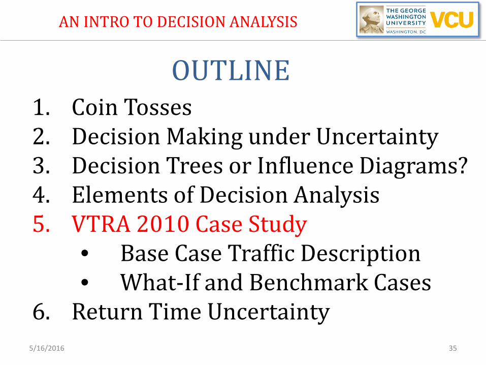
1. Coin Tosses 2. Decision Making under Uncertainty 3. Decision Trees or Influence Diagrams? 4. Elements of Decision Analysis 5. VTRA 2010 Case Study

• Base Case Traffic Description • What-If and Benchmark Cases

6. Return Time Uncertainty 5/16/2016 2

OUTLINE


5/16/2016 3

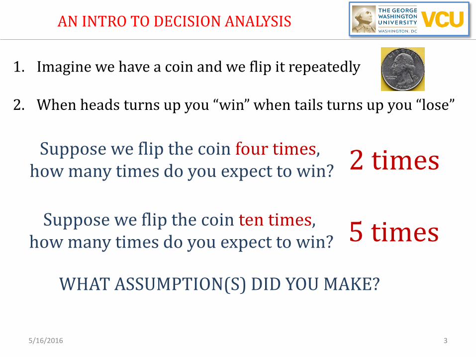
1. Imagine we have a coin and we flip it repeatedly

2. When heads turns up you “win” when tails turns up you “lose”

Suppose we flip the coin four times, how many times do you expect to win?

Suppose we flip the coin ten times, how many times do you expect to win?

2 times

5 times

WHAT ASSUMPTION(S) DID YOU MAKE?


5/16/2016 4

Conclusion: you made reasonable assumptions – 1. The coin has two different sides 2. When flipping it, each side turns up 50% of the time “on average”.

Would it have made sense to assume the coin had only one face

i.e. both sides show heads (or tails)? No

Assuming both sides show heads or tails is equivalent to making

a worst case or best case assumption.


5/16/2016 5

Suppose you actually flip the “fair” coin ten times How many times will “heads” turn up?

Answer could vary from 0 to 10 times, for example, First ten times : 3 times heads turns up Second ten times : 7 times heads turns up Third ten times : 6 times heads turns up Fourth ten times : 4 times heads turns up etc.

We say “on average” 5 out of ten times heads turns up


5/16/2016 6

0% 1%

4%

12%

21%

25%

21%

12%

4%

1% 0%

0%

5%

10%

15%

20%

25%

30%

0 1 2 3 4 5 6 7 8 9 10

Approximately 90% of ten throw series will have 3, 4, 5, 6 or 7 times heads turn up

Conclusion: While we expect 5 times heads to turn up, the actual number is uncertain!


5/16/2016 7

0%

5%

10%

15%

20%

25%

-2 0 2 4 6 8 10 12

Prob

abili

ty

Probabilities for Decision Tree '10 Tosses Coint 1'Optimal Path of Entire Decision Tree

0%

20%

40%

60%

80%

100%

-2 0 2 4 6 8 10 12

Cum

ulat

ive

Prob

abili

ty

Cumulative Probabilities for Decision Tree '10 Tosses Coint 1'Optimal Path of Entire Decision Tree

Probability Node

Risk Profile (RP) – Probability Mass Function (PMF)

Cumulative Risk Profile (CRP) – Cumulative Distribution Function (CDF)

Decision Analysis Software: Precision Tree





OUTLINE


5/16/2016 9

1. Imagine we have two coins: Coin 1 shows heads 50% of the time Coin 2 shows heads 75% of the time

2. When heads turns up, you win a pot of money. When tails turns up, you do not get anything.

You have to choose between Coin 1 and Coin 2 Which one would you choose? Coin 2

WHAT ASSUMPTION DID YOU MAKE? You assumed that the pot of money you win is

the same regardless of the coin you chose!

Coin 1 Coin 2


5/16/2016 10

1. Imagine we have two coins: Coin 1 shows heads 50% of the time Coin 2 shows heads 75% of the time

2. Each time heads turns up, you win the same pot of money. When tails turns up you do not get anything, regardless of the coin you throw.

You have to choose between two alternatives Alternative 1: Throwing ten times with Coin 1 Alternative 2: Throwing five times with Coin 2

Alternative 1 you expect to win 5 times and Alternative 2 you expect to win 3.75 times

Which alternative would you choose? CHOOSE

ALTERNATIVE 1

Coin 1 Coin 2


5/16/2016 11

Our objective is to maximize pay-off. So faced with uncertainty of pay-off outcomes we choose the alternative with largest average pay-off..

Reference Nodes

Decision Node

Probability Nodes

A DECISION TREE: The Basic Risky Decision


5/16/2016 12

0%

20%

40%

60%

80%

100%

-2 0 2 4 6 8 10 12

Cum

ulat

ive

Prob

abili

ty

Cumulative Probabilities for Decision Tree 'Coin Choice'Choice Comparison for Node 'Decision'

Flip Coin 1 10 Times

Flip Coin 2 5 Times

1. Deterministic Dominance 2. Stochastic Dominance 3. Make Decision Based on

Averages

Pr 𝑋 ≤ 𝑥 𝐶𝐶𝐶𝐶 1 ≤ Pr 𝑋 ≤ 𝑥 𝐶𝐶𝐶𝐶 2 ⇕

Pr 𝑋 > 𝑥 𝐶𝐶𝐶𝐶 1 ≥ Pr 𝑋 > 𝑥 𝐶𝐶𝐶𝐶 2

Observe from CRP’s on the Right

Chances of an “Unlucky” Outcome Increase going from 1, 2 to 3

Cumulative Risk Profiles of both Alternatives


5/16/2016 13

1. Imagine we have two coins: Coin 1 shows heads 50% of the time Coin 2 shows heads 75% of the time 2. Each time heads turns up with Coin 1 you win $2. Each time heads turns up with Coin 2 you win $4. When tails turns up you do not get anything.

You have to choose between two ALTERNATIVES Alternative 1: Throwing ten times with Coin 1 Alternative 2: Throwing five times with Coin 2

Alternative 1 you average 5 * $2 = $10 Alternative 2 you average 3.75 * $4 = $15

Which alternative would you choose? CHOOSE

ALTERNATIVE 2

Coin 1 Coin 2


5/16/2016 14

0% 1%4%

12%

21%25%

21%

12%

4%1% 0%0% 1%

9%

26%

40%

24%

0 2 4 6 8 10 12 14 16 18 20

Prob

abili

ty

Pay - Off Outcome

Alternative 1 Alternative 2Average Pay-Off Alt. 1: $10

Average Pay-Off Alt. 2: $15

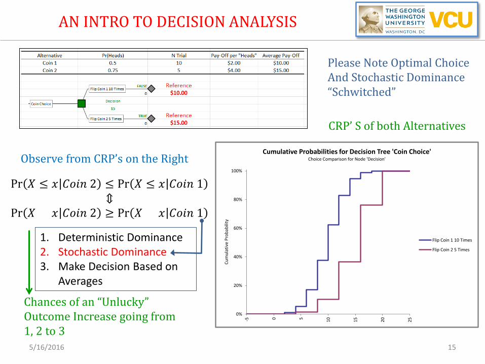
Our objective is to maximize pay-off. So faced with uncertainty of pay-off outcomes we choose the alternative with largest average pay-off.


5/16/2016 15

1. Deterministic Dominance 2. Stochastic Dominance 3. Make Decision Based on

Averages

Pr 𝑋 ≤ 𝑥 𝐶𝐶𝐶𝐶 2 ≤ Pr 𝑋 ≤ 𝑥 𝐶𝐶𝐶𝐶 1 ⇕

Pr 𝑋 > 𝑥 𝐶𝐶𝐶𝐶 2 ≥ Pr 𝑋 > 𝑥 𝐶𝐶𝐶𝐶 1

Observe from CRP’s on the Right

Chances of an “Unlucky” Outcome Increase going from 1, 2 to 3

CRP’ S of both Alternatives

0%

20%

40%

60%

80%

100%

-5 0 5 10 15 20 25

Cum

ulat

ive

Prob

abili

ty

Cumulative Probabilities for Decision Tree 'Coin Choice'Choice Comparison for Node 'Decision'

Flip Coin 1 10 Times

Flip Coin 2 5 Times

Please Note Optimal Choice And Stochastic Dominance “Schwitched”


5/16/2016 16

Conclusion? When choosing between two alternatives entailing a series of coin toss trials, the following comes into play: 1. The number of trials N in each alternative 2. The probability of success P per trial 3. The pay-off amount W per trial

AVERAGE PAY-OFF = N × P × W Is it required to know the absolute value

of N, P and W to choose between these two alternatives?


5/16/2016 17

1. Imagine we have two coins: Coin 2 shows heads 1.5 times more than Coin 1 2. When heads turns up with Coin 2 you win 2 times the amount when heads turns up with Coin 1.

You have to choose between Two Alternatives Alternative 1: Throwing 2*N times with Coin 1 Alternative 2: Throwing N times with Coin 2

Average Pay – Off Alternative 2 : N × 1.5× P × 2 × W Average Pay – Off Alternative 1 : 2 × N × P × W

P = % Heads turns up with Coin 1, W = $ amount you win with Coin 1.

Average Pay-Off Alt. 2/Average Pay-Off Alt. 1 = 1.5


5/16/2016 18

Conclusion? When choosing between two alternatives entailing a series of trials, we can make a

choice if we know the multiplier between the average pay-offs, even when the absolute pay-off values over the two alternatives are unknown/uncertain


1.00

1.20

1.40

1.60

1.80

2.00

2.20

2.40

2.60

2.80

3.00

Pay-

Off

Fact

or

Probability Factor

-20-0 0-20

1.00 1.30 1.60 1.90 2.20 2.502.80

-20

0

20

1.00

1.15

1.30

1.45

1.60

1.75

1.90

Diffe

renc

e in

Pay

-Off

-20-0 0-20

5/16/2016 19

Coin 2 Alternative

Coin 1 Alternative

2D – Strategy Region Diagram



5/16/2016 20

Conclusion? When choosing between two alternatives

entailing a series of trials, we can make a choice if we know the sign of the difference between the average pay-offs, even when only ranges are available for the pay-off probability factors

using a strategy region diagram.


0.00

0.20

0.40

0.60

0.80

1.00

Utili

ty

Pay-Off

5/16/2016 21

What if your Value for Money depends on the amount you win per Coin Toss?


0.00

0.20

0.40

0.60

0.80

1.00

Utili

ty

Pay-Off

Scenario 1: Winning $2 with “Heads” Coin 1

1 at Max

0 at Min

1 at Max

0 at Min

Scenario 2: Winning $20,000 with “Heads” Coin 1

Concave: Risk Averse Linear: Risk Neutral

5/16/2016 22

What if your Value for Money Changes depends on your wealth?


• Linear Utility Function implies the Decision Maker (DM) is Risk Neutral. A DM is Risk Neutral if he/she is indifferent between a bet with an expected pay-off and a sure amount equal to the expected pay-off.

• Concave Utility Function implies a Decision Maker (DM) is Risk Averse. A DM is Risk Averse if he/she is willing to accept less money for a bet with a certain expected pay-off than the expected pay-off.

• Convex Utility Function implies a Decision Maker (DM) is Risk Seeking. A DM is Risk Seeking if he/she is willing to pay more money for a bet with a certain expected pay-off than the expected pay-off.

1.00

1.20

1.40

1.60

1.80

2.00

2.20

2.40

2.60

2.80

3.00

Pay-

Off

Fact

or

Probability Factor

-0.5-0 0-0.5

1.00 1.30 1.60 1.90 2.20 2.502.80

-0.5

0

0.5

1.00

1.15

1.30

1.45

1.60

1.75

1.90

Diffe

renc

e in

Util

ity

-0.5-0 0-0.5

5/16/2016 23

Coin 2 Alternative

Coin 1 Alternative




Now Max. Exp. Utility

5/16/2016 24



0.00

0.20

0.40

0.60

0.80

1.00

Utili

ty

Pay-Off

For how much money are you willing to sell this decision? 0.87

$142,018 Called Certainty Equivalent (CE)

$142,018

Provides for an Operational Interpretation

of the Utility Concept.

< $150,000

5/16/2016 25



0.00

0.20

0.40

0.60

0.80

1.00

Utili

ty

Pay-Off

How much money are you willing to give up to not play?

0.87

$150,000 - $142,018 =

$142,018 < $150,000

$7,982

Called Risk Premium




OUTLINE


5/16/2016 27

Decision Trees or Influence Diagrams?


Lot of Detail, but become Unwieldy

Coin 1 Coin 2

Coin Series Choice

Pay Throw Coin 1

2*N Times

Pay Throw Coin 2

N times

Lack of Detail, Higher level View And Makes Dependence Explicit

Max Pay-Off

5/16/2016 28

Some Basic Influence Diagram Examples


Business Result

Investment Choice

Basic Risky Decision

Arc? Yes or No?

Return on Investment

Source: Clemen and Reilly (2014), Making Hard Decisions, Cengage Learning

5/16/2016 29

Some Basic Influence Diagram Examples


Evacuate?

Imperfect Information

Consequence

Hurricane Path

Weather Forecast

Time Sequence

Arc

Reverse Influence

Arc?


5/16/2016 30

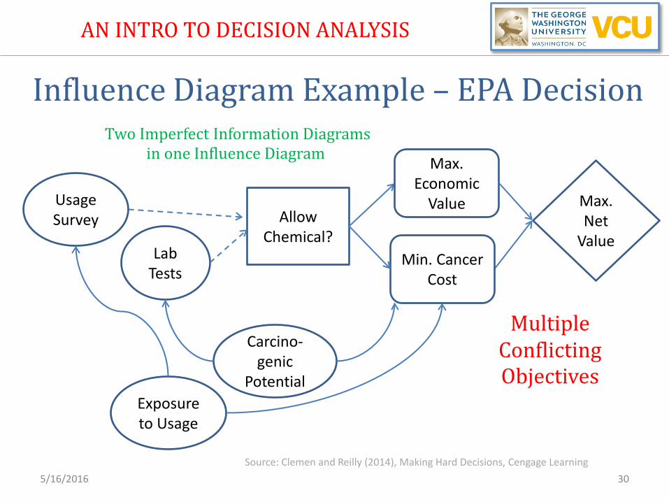
Influence Diagram Example – EPA Decision


Allow Chemical?

Max. Net

Value

Two Imperfect Information Diagrams in one Influence Diagram

Exposure to Usage

Max. Economic

Value

Min. Cancer Cost

Carcino-genic

Potential

Usage Survey

Lab Tests

Multiple Conflicting Objectives


5/16/2016 31


Release 1? Release 2? Final Release?

Current Reliability

Outcome Test 1

Outcome Test 2

Reliability after Test 1

Reliability after Test 2

Profit if released after 1

Cost of Test 1 & Redesign

Profit if released after 2

Cost of Test 2 & Redisgn

Profit if released after final

FINAL PROFITS

Influence Diagram Example – Reliability Growth Decision

Multiple Sequential Decisions




OUTLINE


5/16/2016 33

Elements of Decision Analysis (DA)


• Multiple Decisions: The immediate one and possibly more. Decisions are sequential in time. The DP is called dynamic.

• Multiple Uncertainties: Each uncertainty node requires a probability model. Multiple uncertainty nodes may be statistically dependent.

• Multiple or Single Objectives: In case of multiple conflicting objective the trade-off between objectives needs to be modelled.

• Multiple values: Evaluation of achievements of each individual objective requires description of a utility function for each one

(linear, concave, convex?)

DA’s are Complex!

5/16/2016 34

Skill Set/Techniques for Decision Analysis (DA)


• Decision Tree/Influence Diagrams: To structure and visualize DP’s, identify its elements and prescribe the method towards evaluation.

• Expert Judgement (EJ) Elicitation: To describe/specify probability models of “on-off” uncertainty nodes and to combine expert judgements.

• Statistical Inference: In DA the inference is typically Bayesian in nature. Is used when uncertainties reveal themselves over time to refine/update probability models or combine available data with Expert Judgement.

• Utility Theory: To describe “The Decision Maker’s” risk attitude/ appetite for the evaluation of a single objective and to formalize trade-off between multiple objectives.

Thus, a DA’s is Normative in Nature !




OUTLINE


5/16/2016 36

IMAGES FROM THE SALISH SEA

VESSEL TRAFFIC RISK ASSESSMENT (VTRA) 2010

5/16/2016 37

VTRA 2010 Study Area

• Kinder Morgan: + 348 Tankers • Delta Port: + 348 Cont. & 67 Bulkers

• Gateway: + 487 Bulkers


5/16/2016 38

• BP Cherry Point Refinery • Ferndale Refinery • March Point Refinery

VTRA 2010 Study Area


5/16/2016 39

What was The Objective in Coin Toss Example? Maximize Average Pay-Off

What is the Objective in a Maritime Risk Assesment? Minimize Average Potential Oil Loss

Truth be told, for some the objective is to Maximize Average Pay-Off, for some it is to Minimize Average Potential Oil Loss

and for others it is to Achieve Both.

For sake of argument, lets take in Maritime Risk Assessment a focus towards Minimizing Average Potential Oil Loss, while

recognizing the Maximize Average Pay-Off Objective is also at play.

ciii xlsR },,{ ><=Risk Analysis Objective: Evaluate Oil Spill System Risk described by a “complete” set of traffic situations

Situations Incidents Accidents Oil Spill

Maritime Simulation

Traffic Situations

Expert Judgment + Data

Incident Data

Likelihoods

Oil Outflow Model

Consequences


An Oil Spill is a series of cascading events referred to as a Causal Chain

Coin Toss Analogy: Trials % of Heads (P) Winnings ($) Pay-off Risk was defined by N identical Trials

5/16/2016 40


5/16/2016 41

VTRA 2010 Analysis Approach In light of uncertainties inherent to any risk analysis, we choose not to focus on; • absolute evaluations of risk levels, but to focus on • relative risk changes from a base case scenario by adding or removing traffic to or from that base case.


5/16/2016 42

VTRA 2010 Analysis Approach A Base Case (BC) Analysis Framework is constructed while; • making reasonable assumptions (not worst or best case), and • What-if (WI), Bench-Mark (BM) and Risk Mitigation Measure (RMM) cases are analyzed within that framework.

• Base Case (BC) system wide risk levels are set at 100%, and • System wide % changes up or down are evaluated for What-if (WI), Bench-Mark (BM) and Risk Mitigation Measure (RMM), moreover • Location-Specific Multipliers are evaluated for 15 Waterway Zones.


5/16/2016 43

VTRA 2010 Analysis Approach


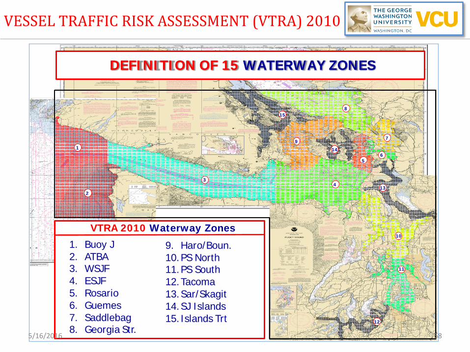
DEFINITION OF 15 WATERWAY ZONES

65

7

8

9

15

43

1

213

10

11

12

1. Buoy J2. ATBA3. WSJF4. ESJF5. Rosario6. Guemes7. Saddlebag8. Georgia Str.

9. Haro/Boun.10.PS North11.PS South12.Tacoma13.Sar/Skagit14.SJ Islands15.Islands Trt

VTRA 2010 Waterway Zones

14

5/16/2016 44

45

A B

C D

E F

Generating Traffic Situations:

Counting Collision Accident Scenario’s

Counting Drift Grounding Accident Scenario’s

Counting Powered Grounding Accident Scenario’s

5/16/2016 GW-VCU : DRAFT 45


5/16/2016 46

VTRA 2010 Analysis Approach • Map is divided in squares of grid cells with dimension half nautical mile by half nautical mile and The VTRA 2010

Evaluates per Grid Cell! • # of traffic situations per year • potential accident frequency per year • potential oil loss per year

B A 5/16/2016 47


ciii xlsR },,{ ><=

Risk Assessment: Traffic Situations Likelihoods Consequences

Oil Spill System Risk is described by “complete” set of traffic situations

EVALUATE AVERAGE PAY-OFF = N × P × W

EVALUATE AVERAGE VESSEL TIME EXPOSURE

EVALUATE AVERAGE OIL TIME EXPOSURE

EVALUATE AVERAGE ANNUAL POTENTIAL ACC. FREQ.

EVALUATE AVERAGE ANNUAL POTENTIAL OIL LOSS

Display results visually in 2D and 3D geographic profiles

Driver for

Driver for

Recall Coin Toss Analogy: Trials (N) % of Heads (P) Winnings (W)

Per Grid Cell!!

5/16/2016 48


5/16/2016 49

VTRA 2010 Analysis Approach Collision System Exposure in Base Case:

• Approximately 10,000 grid cells of 0.5 x 0.5 mile in VTRA study area with Vessel to Vessel traffic situations. • Approximately 1.8 Million Vessel to Vessel Traffic Situations per year generated by VTRA 2010 Model. • Vessel to Vessel Traffic Situations per cell per year range from 1 – 7,000 (or on average about 0 – 20 per day per cell) .

Recall Coin Toss – Traffic Situation Analogy: “1.8 Million Coin Tosses with very small probability of Tails”


5/16/2016 50

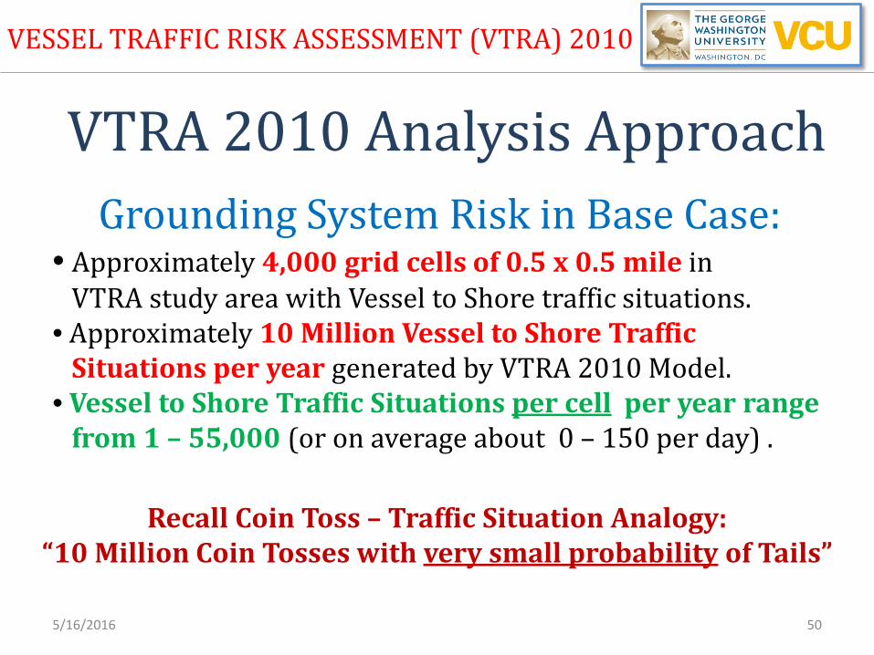
VTRA 2010 Analysis Approach Grounding System Risk in Base Case:

• Approximately 4,000 grid cells of 0.5 x 0.5 mile in VTRA study area with Vessel to Shore traffic situations. • Approximately 10 Million Vessel to Shore Traffic Situations per year generated by VTRA 2010 Model. • Vessel to Shore Traffic Situations per cell per year range from 1 – 55,000 (or on average about 0 – 150 per day) .

Recall Coin Toss – Traffic Situation Analogy: “10 Million Coin Tosses with very small probability of Tails”

1. Coin Tosses 2. Decision Making under Uncertainty 3. Decision Trees or Influence Diagrams 4. Elements of Decision Analysis 5. VTRA 2010 Case Study



OUTLINE



P: Base Case 3D Risk Profile MAP TO DISPLAY - Vessel Time Exposure

23-24 22-23

21-22 20-21

19-20 18-19

17-18 16-17

15-16 14-15

13-14 12-13

11-12 10-11

9-10 8-9

7-8 6-7

5-6 4-5

3-4 2-3

1-2 0-1

Neah Bay

Victoria Seattle

Bellingham

Tacoma

VESSEL TIME EXPOSURE (VTE) = Annual amount of time a location is exposed to a vessel moving through it

5/16/2016 52

P: Base Case 3D Risk Profile ALL TRAFFIC - Vessel Time Exposure: 100%Total VTE

23-24 22-23

21-22 20-21

19-20 18-19

17-18 16-17

15-16 14-15

13-14 12-13

11-12 10-11

9-10 8-9

7-8 6-7

5-6 4-5

3-4 2-3

1-2 0-1

ALL VTRA TRAFFIC – VTOSS 2010 TRAFFIC + SMALL VESSEL EVENTS


Neah Bay

Victoria Seattle

Bellingham

Tacoma

VESSEL TIME EXPOSURE (VTE) = Annual amount of time a location is exposed to a vessel moving through it

5/16/2016 53

P: Base Case 3D Risk Profile NON FV - Vessel Time Exposure: 75%Total VTE

23-24 22-23

21-22 20-21

19-20 18-19

17-18 16-17

15-16 14-15

13-14 12-13

11-12 10-11

9-10 8-9

7-8 6-7

5-6 4-5

3-4 2-3

1-2 0-1

2010 NON FV – 75% of 2010 Total

NON – FV TRAFFIC

+

41.3% - FISHINGVESSEL 18.1% - FERRY 06.8% - BULKCARGOBARGE 06.0% - UNLADENBARGE 04.0% - YACHT 03.9% - NAVYVESSEL 03.3% - TUGNOTOW 02.8% - FERRYNONLOCAL 02.7% - PASSENGERSHIP 02.2% - WOODCHIPBARGE

02.1% - LOG_BARGE 01.7% - TUGTOWBARGE 01.5% - USCOASTGUARD 01.1% - FISHINGFACTORY 00.8% - RESEARCHSHIP 00.7% - OTHERSPECIFICSERV 00.6% - CONTAINERBARGE 00.2% - SUPPLYOFFSHORE 00.2% - CHEMICALBARGE 00.0% - DERRICKBARGE


Neah Bay

Victoria Seattle

Bellingham

Tacoma

5/16/2016 54

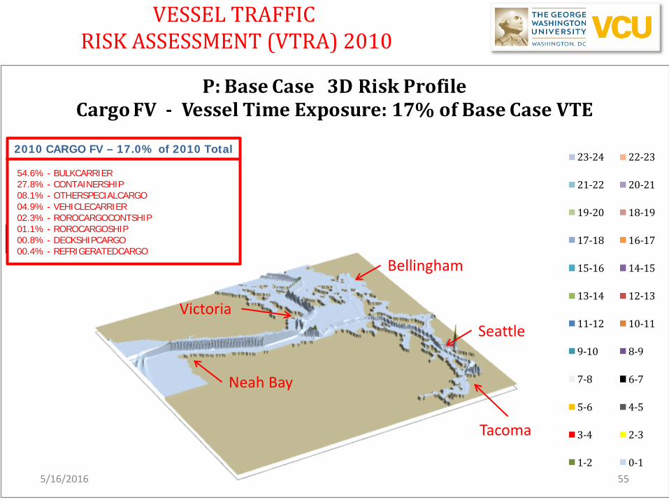
P: Base Case 3D Risk Profile Cargo FV - Vessel Time Exposure: 17% of Base Case VTE

23-24 22-23

21-22 20-21

19-20 18-19

17-18 16-17

15-16 14-15

13-14 12-13

11-12 10-11

9-10 8-9

7-8 6-7

5-6 4-5

3-4 2-3

1-2 0-1


+ 100.0% of Base

Neah Bay

Seattle

Bellingham

Tacoma

Victoria

2010 CARGO FV – 17.0% of 2010 Total

54.6% - BULKCARRIER 27.8% - CONTAINERSHIP 08.1% - OTHERSPECIALCARGO 04.9% - VEHICLECARRIER 02.3% - ROROCARGOCONTSHIP 01.1% - ROROCARGOSHIP 00.8% - DECKSHIPCARGO 00.4% - REFRIGERATEDCARGO

5/16/2016 55

P: Base Case 3D Risk Profile Tank FV - Vessel Time Exposure: 8% of Base Case VTE

23-24 22-23

21-22 20-21

19-20 18-19

17-18 16-17

15-16 14-15

13-14 12-13

11-12 10-11

9-10 8-9

7-8 6-7

5-6 4-5

3-4 2-3

1-2 0-1


Neah Bay

Seattle

Bellingham

Tacoma

Victoria

+ 100.0% of Base

2010 TANK FV – 8% of 2010 Total

54.5% - OILBARGE 24.4% - OILTANKER 11.3% - CHEMICALCARRIER 09.8% - ATB

5/16/2016 56


5/16/2016 57

P: Base Case 3D Risk Profile All FV - Vessel Time Exposure: 100% of Base Case VTE

23-24 22-23

21-22 20-21

19-20 18-19

17-18 16-17

15-16 14-15

13-14 12-13

11-12 10-11

9-10 8-9

7-8 6-7

5-6 4-5

3-4 2-3

1-2 0-1

ALL FV (100%) Bulk Carriers (≈33%) Container Ships (≈20%) Other Cargo (≈13%) Oil Tankers (≈9%) Chemical Carriers (≈4%) Oil Barges (≈19%) ATB’s (≈3%)

FV = Focus Vessel

FV TRAFFIC ACCOUNTS FOR (≈25%) OF TOTAL TRAFFIC

Where do Focus Vessels Travel?

Neah Bay

Seattle

Bellingham

Tacoma

Victoria

GW-VCU : DRAFT 57


P: Base Case 3D Risk Profile Tanker - Vessel Time Exp.: 9% of Base Case VTE

23-24 22-23

21-22 20-21

19-20 18-19

17-18 16-17

15-16 14-15

13-14 12-13

11-12 10-11

9-10 8-9

7-8 6-7

5-6 4-5

3-4 2-3

1-2 0-1

March Point

Cherry Point

Ferndale

Port Angeles

ALL FV Bulk Carriers Container Ships Other Cargo Oil Tankers (≈9%) Chemical Carriers Oil Barges ATB’s

FV = Focus Vessel

Where do Tankers Travel?

5/16/2016 58


P: Base Case 3D Risk Profile MAP TO DISPLAY - Oil Time Exposure

23-24 22-23

21-22 20-21

19-20 18-19

17-18 16-17

15-16 14-15

13-14 12-13

11-12 10-11

9-10 8-9

7-8 6-7

5-6 4-5

3-4 2-3

1-2 0-1

P: Base Case 3D Risk Profile MAP TO DISPLAY - Vessel Time Exposure

23-24 22-23

21-22 20-21

19-20 18-19

17-18 16-17

15-16 14-15

13-14 12-13

11-12 10-11

9-10 8-9

7-8 6-7

5-6 4-5

3-4 2-3

1-2 0-1

Neah Bay

Victoria Seattle

Bellingham

Tacoma

OIL TIME EXPOSURE (OTE) = Annual amount of time a location is exposed to a cubic meter of oil moving through it

Oil

5/16/2016 59

P: Base Case 3D Risk Profile All FV - Oil Time Exposure: 100% of Base Case OTE

23-24 22-23

21-22 20-21

19-20 18-19

17-18 16-17

15-16 14-15

13-14 12-13

11-12 10-11

9-10 8-9

7-8 6-7

5-6 4-5

3-4 2-3

1-2 0-1


March Point

Cherry Point Ferndale

Port Angeles

Where does Oil on Focus Vessels Travel?

FV = Focus Vessel

ALL FV (100%) Bulk Carriers (≈8%) Container Ships (≈9%) Other Cargo (≈3%) Oil Tankers (≈48%) Chemical Carriers (≈9%) Oil Barges (≈21%) ATB’s (≈3%)

5/16/2016 60


P: Base Case 3D Risk Profile Tanker - Oil Time Exposure: 48% of Base Case OTE

23-24 22-23

21-22 20-21

19-20 18-19

17-18 16-17

15-16 14-15

13-14 12-13

11-12 10-11

9-10 8-9

7-8 6-7

5-6 4-5

3-4 2-3

1-2 0-1

March Point

Cherry Point Ferndale

Port Angeles

Where does Oil on board Tankers Travel? ALL FV (100%) Bulk Carriers Container Ships Other Cargo Oil Tankers (≈48%) Chemical Carriers Oil Barges ATB’s

FV = Focus Vessel

5/16/2016 61




OUTLINE


BUNKERING SUPPORT ROUTES

DP415: 348 BULK CARRIERS + 67 CONTAINER SHIPS + Bunkering Support


5/16/2016 63

GW487: + 487 BULK CARRIERS + Bunkering Support

KM348: + 348 TANKERS + Bunkering Support

WHAT – IF SCENARIO ROUTES


BENCH-MARK TANKER ROUTES P: BC & HIGH TAN 3D Risk Profile

What-If FV - Vessel Time Exp.: 2% of Base Case VTE

23-24 22-23

21-22 20-21

19-20 18-19

17-18 16-17

15-16 14-15

13-14 12-13

11-12 10-11

9-10 8-9

7-8 6-7

5-6 4-5

3-4 2-3

1-2 0-1

+ 142 Tankers added to Base Case (2007 Historical High Year)

5/16/2016 64

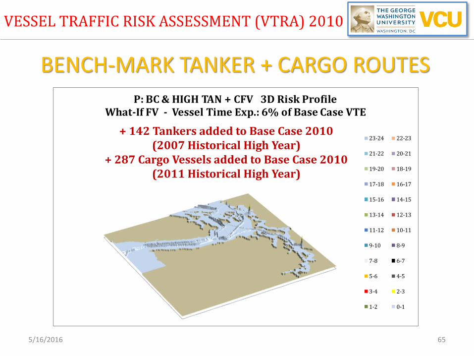
P: BC & HIGH TAN + CFV 3D Risk Profile What-If FV - Vessel Time Exp.: 6% of Base Case VTE

23-24 22-23

21-22 20-21

19-20 18-19

17-18 16-17

15-16 14-15

13-14 12-13

11-12 10-11

9-10 8-9

7-8 6-7

5-6 4-5

3-4 2-3

1-2 0-1


BENCH-MARK TANKER + CARGO ROUTES

+ 142 Tankers added to Base Case 2010 (2007 Historical High Year)

+ 287 Cargo Vessels added to Base Case 2010 (2011 Historical High Year)

5/16/2016 65


WHAT – IF SCENARIO ANALYSES

Vessel Time Exposure (VTE)

Oil Time Exposure (OTE)

Pot. Accident Frequency (PAF)

Pot. Oil Loss (POL)

P - Base Case 100% 100% 100% 100%

P - Base Case

Q - GW - 487

R - KM - 348

S - DP - 415

T - GW - KM - DP




Pot. Oil Loss (POL)

P - Base Case 100% 100% 100% 100%

Q - GW - 487 +13% | 113% +5% | 105% +12% | 112% +12% | 112%

R - KM - 348 +7% | 107% +51% | 151% +5% | 105% +36% | 136%

S - DP - 415 +5% | 105% +3% | 103% +6% | 106% +4% | 104%

T - GW - KM - DP +25% | 125% +59% | 159% +18% | 118% +68% | 168%

WHAT IF SCENARIO ANALYSIS


Combined expansion scenario of above three expansion scenarios


Modeled Base Case 2010 year informed by VTOSS 2010 data amongst other sources.

Gateway expansion scenario with 487 additional bulk carriers and bunkering support

Transmountain pipeline expansion with additional 348 tankers and bunkering support

Delta Port Expansion with additional 348 bulk carriers and 67 container vessels

5/16/2016 66


BENCH MARK ANALYSES ON BASE CASE


Oil Time Exposure (OTE)Pot. Accident Frequency

(PAF)Pot. Oil Loss (POL)

P - Base Case 100% 100% 100% 100%

P - Base Case

P - BC & LOW TAN + CFV

P - BC & LOW TAN

P - BC & HIGH TAN

P - BC & HIGH TAN + CFV




Pot. Oil Loss (POL)

P - Base Case 100% 100% 100% 100%P - BC & LOW TAN + CFV -3% | 97% -14% | 86% -5% | 95% -20% | 80%

P - BC & LOW TAN -2% | 98% -13% | 87% -4% | 96% -22% | 78%

P - BC & HIGH TAN +2% | 102% +14% | 114% +3% | 103% +9% | 109%

P - BC & HIGH TAN + CFV +7% | 107% +15% | 115% +4% | 104% +8% | 108%

CASE P BENCHMARK (BM) & SENSITIVITY ANALYSIS

Base Case with Tankers and Cargo Focus Vessels set at a high historical year

P - RMM SCENARIO REFERENCE POINT

CASE P BENCHMARK (BM) & SENSITIVITY ANALYSIS

Base Case with Tankers and Cargo Focus Vessels set at a low historical year

Base Case with Tankers set at a low historical year

Base Case with Tankers set at a high historical year

Modeled Base Case 2010 year informed by VTOSS 2010 data amongst other sources.

5/16/2016 67


DEFINITION OF 15 WATERWAY ZONES

65

7

8

9

15

43

1

213

10

11

12

1. Buoy J2. ATBA3. WSJF4. ESJF5. Rosario6. Guemes7. Saddlebag8. Georgia Str.

9. Haro/Boun.10.PS North11.PS South12.Tacoma13.Sar/Skagit14.SJ Islands15.Islands Trt

VTRA 2010 Waterway Zones

14

5/16/2016 68


0.1%

0.2%

0.2%

0.4%

0.6%

3.9%

4.8%

4.8%

9.8%

9.8%

10.0%

10.0%

13.4%

14.9%

17.0%

0.3%

0.2%

0.2%

0.4%

2.5%

7.1%

6.5%

9.8%

46.7%

23.8%

10.3%

10.0%

12.6%

15.5%

22.3%

0.0% 10.0% 20.0% 30.0% 40.0% 50.0%

SJ Islands : +0.2% | x 2.89Sar/Skagit : 0.0% | x 0.93

ATBA : 0.0% | x 0.93Tac. South : +0.0% | x 1.00

Buoy J : +1.9% | x 4.44Georgia Str. : +3.2% | x 1.81Islands Trt : +1.8% | x 1.38

WSJF : +5.0% | x 2.04Haro/Boun. : +36.9% | x 4.75

ESJF : +13.9% | x 2.42PS North : +0.3% | x 1.03

PS South : 0.0% | x 1.00Saddlebag : -0.8% | x 0.94

Rosario : +0.5% | x 1.03Guemes : +5.3% | x 1.31

% Base Case Pot. Oil Loss (POL) - ALL_FV

Comparison of Potential Oil Loss by Waterway Zone

T: GW - KM - DP : 168% ( +68.2% | x 1.68) P: Base Case : 100%

++68%

Zone: Diff. | Factor

CASE-T5/16/2016 69


RISK MITIGATION ANALYSES ON CASE T

5/16/2016 70




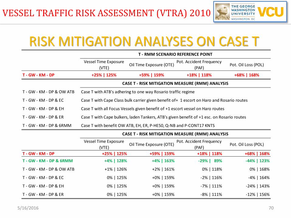
T - GW - KM - DP +25% | 125% +59% | 159% +18% | 118% +68% | 168%

T - GW - KM - DP & OW ATB

T - GW - KM - DP & EC

T - GW - KM - DP & EH

T - GW - KM - DP & ER

T - GW - KM - DP & 6RMM




T - GW - KM - DP +25% | 125% +59% | 159% +18% | 118% +68% | 168%T - GW - KM - DP & 6RMM +4% | 128% +4% | 163% -29% | 89% -44% | 123%

T - GW - KM - DP & OW ATB +1% | 126% +2% | 161% 0% | 118% 0% | 168%

T - GW - KM - DP & EC 0% | 125% +0% | 159% -2% | 116% -4% | 164%

T - GW - KM - DP & EH 0% | 125% +0% | 159% -7% | 111% -24% | 143%

T - GW - KM - DP & ER 0% | 125% +0% | 159% -8% | 111% -12% | 156%

CASE T - RISK MITIGATION MEASURE (RMM) ANALYSIS

T - RMM SCENARIO REFERENCE POINT

Case T with all Focus Vessels given benefit of +1 escort vessel on Haro routes

Case T with Cape bulkers, laden Tankers, ATB's given benefit of +1 esc. on Rosario routes

Case T with benefit OW ATB, EH, ER, P-HE50, Q-NB and P-CONT17 KNTS

CASE T - RISK MITIGATION MEASURE (RMM) ANALYSIS

Case T with ATB's adhering to one way Rosario traffic regime

Case T with Cape Class bulk carrier given benefit of+ 1 escort on Haro and Rosario routes




OUTLINE


5/16/2016 72

VTRA 2010 Analysis Approach The ORIGINAL VTRA 2010 Study

did not evaluate average accident return times as its risk metric of choice.

Other Maritime Risk Studies, however, do evaluate average accident return times

as its risk metric of choice. I am presenting this type of analysis here

to allow for a comparison between these studies.

SUPPLEMENT ANALYSIS - VESSEL TRAFFIC RISK ASSESSMENT (VTRA) 2010

5/16/2016 73

Why did we not use average return times as risk metric of choice?

Imagine we have had two accidents in a calendar year and we would like to evaluate the “average return time” over that year

Jan Feb Mar Apr May June July Aug Sep Oct Nov Dec

Accident Accident

What is the value of the “average return time”?

3 months > 5 months > 4 months

> (4 + 3 + 5)/3 = 4 Months!!!


5/16/2016 74


The prevailing wisdom, however, converts 2 accidents/year to

an “average return time” of ½ year = 6 months

Jan Feb Mar Apr May June July Aug Sep Oct Nov Dec

Accident Accident

6 months 6 months

Accident


5/16/2016 75

Conclusion? The definition: Average Return Time = 1 / # Accidents per Year

Assumes that accidents are equally spaced, which they are not!!!


Some would argue: “It’s an average and thus this evens out in the long run”

This would only be true if # Accidents per year is large, which does not apply

to low probability – high consequence events!!!


5/16/2016 76


# Accidents per year Average Return TimeYear 1 1 12 monthsYear 2 4 3 monthsYear 3 4 3 months

Average 3 6 months

“Average Return Time” = 1 / # Accidents per Year

But: 1/3 year = 4 months

Conclusion? 1/ Average (# Accidents per Year) < Average (Average Return Time)

Suppose you have multiple years of data

Both methods are used to evaluate average return times which only adds to confusion!


5/16/2016 77

Evaluating average return uncertainty Recall VTRA 2010 Maritime Simulation Model generated • 1.8 Million Vessel to Vessel Traffic Situations per Year • 10 Million Vessel to Shore Traffic Situations per Year

Accident Probability per Traffic Situation

(1000 - 7500] (7500 - 15000] (15000 or More)

1 e -10 N1 N2 N3

1 e -9 N4 N5 N6

1 e -8 N7 N8 N9

POTENTIAL OIL LOSS VOLUME (m3) CATEGORY

Used VTRA 2010 Model to create table of following format


5/16/2016 78

Evaluating average return uncertainty

Accident Probability per Traffic Situation

(1000 - 7500] (7500 - 15000] (15000 or More)

1 e -10 N1 N2 N3

1 e -9 N4 N5 N6

1 e -8 N7 N8 N9

POTENTIAL OIL LOSS VOLUME (m3) CATEGORY

Recall coin Toss Analogy

“Trials” “Probability of Tails”

Sample # Accidents per year using Coin Toss Analogies

Step 1

Set Average Return Time = 1/ # Accidents per year

Step 2

Repeat Step 1 and Step 2 (2500 Samples)


0

0.25

0.5

0.75

1

0 20 40 60 80 100 120

Cum

ulat

ive

Pere

cent

age

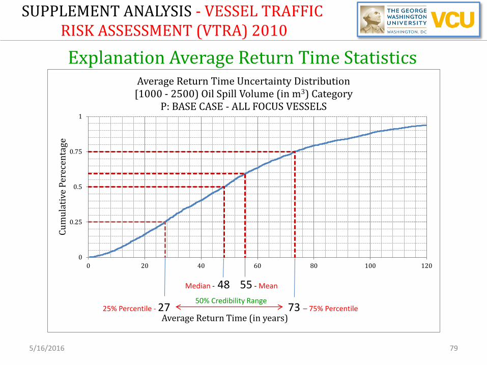
Average Return Time (in years)

Average Return Time Uncertainty Distribution [1000 - 2500) Oil Spill Volume (in m3) Category

P: BASE CASE - ALL FOCUS VESSELS


5/16/2016 79

25% Percentile - 27 73 – 75% Percentile 50% Credibility Range

Median - 48 55 - Mean

Explanation Average Return Time Statistics

WI - SCEN

(15000 - M

ore]

(12500 - 1

5000]

(10000 - 1

2500]

(7500 - 1

0000]

(5000 - 7

500]

(2500 - 5

000]

(1000 - 2

500]R - K

M348P - B

C

R - KM348

P - BC

R - KM348

P - BC

R - KM348

P - BC

R - KM348

P - BC

R - KM348

P - BC

R - KM348

P - BC

3000

2500

2000

1500

1000

500

0Aver

age

Retu

rn T

ime

(Yrs

)

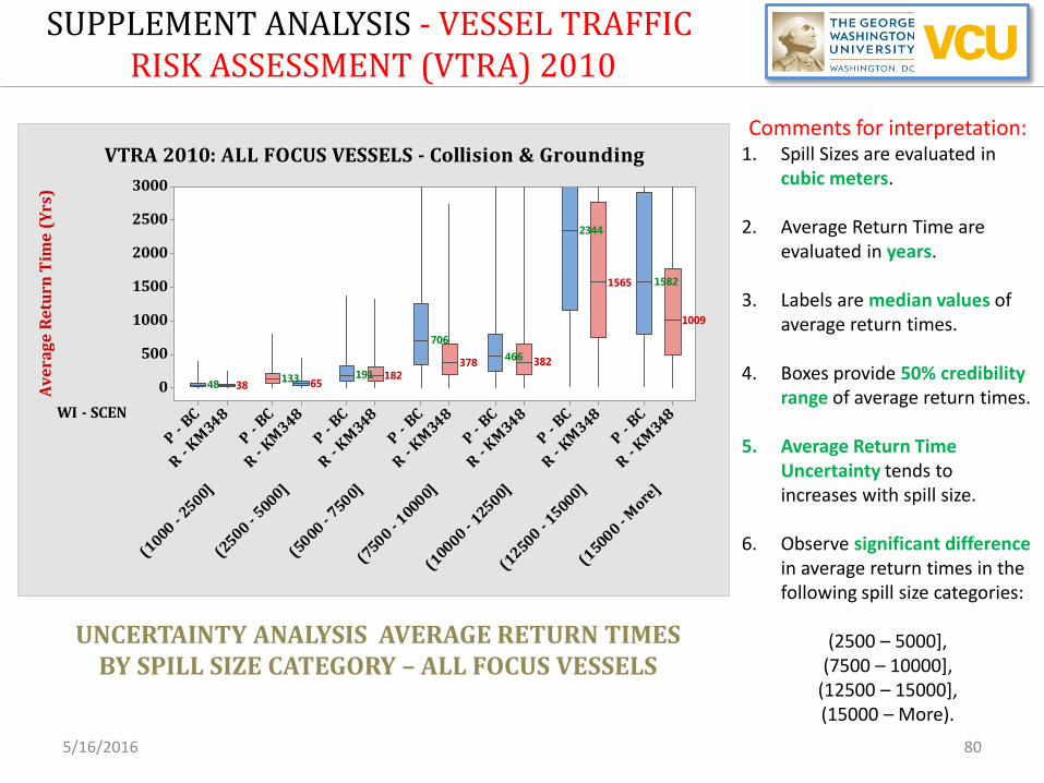
3848 65133 182191378

706

382466

1565

2344

1009

1582

VTRA 2010: ALL FOCUS VESSELS - Collision & Grounding


5/16/2016 80

Comments for interpretation: 1. Spill Sizes are evaluated in

cubic meters.

2. Average Return Time are evaluated in years.

3. Labels are median values of average return times.

4. Boxes provide 50% credibility range of average return times.

5. Average Return Time Uncertainty tends to increases with spill size.

6. Observe significant difference in average return times in the following spill size categories:

(2500 – 5000], (7500 – 10000],

(12500 – 15000], (15000 – More).

UNCERTAINTY ANALYSIS AVERAGE RETURN TIMES BY SPILL SIZE CATEGORY – ALL FOCUS VESSELS


QUESTIONS?

5/16/2016 81

what do coin tosses, decision making under uncertainty ... · jason r.w. merrick (vcu) and j. rene...

Documents