P A P E R

What can strike-slip fault spacing tell us about the plateboundary of western North America?

Andrew V. Zuza | Chad W. Carlson

Nevada Bureau of Mines and Geology,

University of Nevada, Reno, NV, USA

Correspondence

Andrew V. Zuza, Nevada Bureau of Mines

and Geology, University of Nevada, Reno,

NV, USA.

Email: azuza@unr.edu; avz5818@gmail.com

Funding information

University of Nevada, Reno

Abstract

The spacing of parallel continental strike-slip faults can constrain the mechanical

properties of the faults and fault-bounded crust. In the western US, evenly spaced

strike-slip fault domains are observed in the San Andreas (SA) and Walker Lane (WL)

fault systems. Comparison of fault spacing (S) vs. seismogenic zone thickness (L) rela-

tionships of the SA and WL systems indicates that the SA has a higher S/L ratio (~8

vs. 1, respectively). If a stress-shadow mechanism guides parallel fault formation, the

S/L ratio should be controlled by fault strength, crustal strength, and/or regional

stress. This suggests that the SA-related strike-slip faults are relatively weaker, with

lower fault friction: 0.13–0.19 for the SA vs. 0.20 for WL. The observed mechanical

differences between the San Andreas and Walker Lane fault systems may be attribu-

ted to variations in the local geology of the fault-hosting crust and/or the regional

boundary conditions (e.g. geothermal gradient or strain rate).

1 | INTRODUCTION

Parallel strike-slip faults are observed at a variety of scales, from

continental faults that cut through the entire brittle crust to millime-

ter-scale faults in outcrops and analogue experiments (Davy & Cob-

bold, 1988; Dickinson, 1996; Martel & Pollard, 1989; Segall &

Pollard, 1983). Analyses of active strike-slip faults in central Asia and

California suggest that a modified stress-shadow mechanism

(Lachenbruch, 1961) controls fault spacing (Yin, Zuza, & Pappalardo,

2016; Zuza, Yin, Lin, & Sun, 2017). Accordingly, the characteristic

fault spacing (S) is linearly related to the brittle-layer thickness (h)

(i.e. the seismogenic zone) of a deforming layer as a function of fault

strength, crustal strength, and regional stress.

We examined parallel strike-slip fault domains along the western

plate boundary of North America to understand the development of

the San Andreas (SA) and Walker Lane (WL) fault systems (Figure 1)

in the context of continental-scale stress shadows. These faults are

ideal because they (1) are part of the same plate boundary with simi-

lar kinematics, (2) are under similar overall stress state, and (3) repre-

sent both mature (i.e. SA) and incipient (i.e. WL) plate-boundary

faults systems (Atwater, 1970; DeMets, Gordon, Stein, & Argus,

1987; Faulds, Henry, & Hinz, 2005; Wesnousky, 2005).

2 | STRESS-SHADOW MODEL

We use a stress-shadow model to describe the formation of parallel

strike-slip faults (Lachenbruch, 1961; Pollard & Segall, 1987) (Fig-

ure 2). This model assumes that the crust is under some remote

shear stress rrs that exceeds the shear-fracture strength of the

deforming crust Y, causing strike-slip fault formation. The presence

of the fault imposes a local low-stress boundary condition, as the

shear stress rs decreases to the fault-plane shear stress rf (Figure 2).

Moving away from the fault, rs rises toward rrs, and the distance

from the fault when rs ≥ Y is the stress-shadow length S. A new

strike-slip fault is expected to form only at a distance >S from a pre-

viously formed fault (Figure 2).

Detailed stress-shadow derivations are provided in Zuza et al.

(2017). In this model, the deforming crust behaves as a perfectly

plastic medium at the depth- and time-scales of interest. Rock defor-

mation may behave elastically in lower-stress conditions but once

stress exceeds the elastic limit of the crust, non-recoverable plastic

deformation occurs (Figure 3). With a high enough stress magnitude,

brittle failure occurs following the Coulomb-fracture criterion (Fig-

ure 3). We ignore the low-strain elastic deformation and model the

deforming crust as completely plastic, controlled by the Coulomb-

Received: 12 May 2017 | Revised: 24 August 2017 | Accepted: 7 November 2017

DOI: 10.1111/ter.12315

Terra Nova. 2017;1–9. wileyonlinelibrary.com/journal/ter © 2017 John Wiley & Sons Ltd | 1

fracture criterion (Figure 3). We also assume that crustal strength

resides dominantly in the brittle crust (Jackson, McKenzie, Priestley,

& Emmerson, 2008; Lister & Davis, 1989). Thus, crustal stress and

strength are approximately linearly depth dependent (Figure 3). Brit-

tle-crust thickness may be constrained by empirical and theoretical

yield envelopes (Goetze & Evans, 1979), but parameter variability

San Francisco

SacramentoCarson City

Reno

Bakersfield

Los Angeles

Santa Barbara

San Diego

Las Vegas

Eastern CAshear zone

15 ± 5 km

12 ± 2 km

10 ± 3 km

14 ± 4 km33 ± 3 km

47 ± 15 km

16 ± 2 km

20 ± 8 km

Right-slip faults in redLeft-slip faults in blue

100 km

120°W

40°NWalker Lane

San Andreas fault system

NorthernCalifornia

Western S.California

Mojave

E. Transverse

Mina Deflection

Walker LakeCarson

Pyramid Lake

F IGURE 1 Parallel strike-slip faultdomains (Faulds & Henry, 2008; Stewart,1988) in the San Andreas and Walker Lanefault systems (Faulds & Henry, 2008;Wesnousky et al., 2012). Numberscorrespond to average spacing (Zuza et al.,2017; this study). Inset shows the namesof each strike-slip fault domain

H = αh h = hf

hfv

L = hf + hfv

σs

y

x

z σs (x = S) = Yσs (x = ∞) = σs

r

σs(x = –S) = Yσf

Y

S

Preferential sites of new fault formation

S Ductile lower crustSemi-brittle

Mantle lithosphere

Brittle upper crust

Strong bounding region where σs= σs

r

σsr

Strong bounding region where σs= σs

r

Shear stress on fault plane σf

frictional sliding

viscous creep

transitional

F IGURE 2 Model for parallel strike-slip fault formation via the stress-shadow mechanism, modified from Zuza et al. (2017). The boundaryconditions rs(x = 0) = rf and rs (x = ∞) = rr

s are satisfied by off-fault shear stress rs. Parameters: rf: shear stress on the fault; rf : verticallyaveraged shear strength of the fault; rr

s: regional shear stress in the brittle crust; S: stress-shadow length equal to fault spacing; Y: shear-fracture strength of the deforming strike-slip fault domain; h: brittle-crust thickness in the region of strike-slip faulting; H: brittle-crustthickness of the stronger bounding region; L: seismogenic zone thickness, including regimes of frictional sliding (hf) and transitional frictionalsliding and viscous creep (hfv); a = H/h

2 | ZUZA AND CARLSON

(e.g. grain size or strain rate) and a potentially diffuse brittle–ductile

transition zone (Carter & Tsenn, 1987; Pec, St€unitz, Heilbronner, &

Drury, 2016) make these estimates imprecise. Here, we use the seis-

mogenic zone to approximate the brittle-crust thickness (Chiarabba

& De Gori, 2016; Nazareth & Hauksson, 2004; Williams, 1996).

Previous analyses of fault spacing S and brittle-layer thickness h

in California, central Asia, and scaled analogue experiments showed

that S and h are linearly related (Zuza et al., 2017). The simplified,

linear stress-shadow solution for parallel strike-slip fault formation is:

S ¼�Y � rf

rrs � �Y

h (1)

where �Y and rf are the vertically averaged shear-fracture strength

of the deforming brittle crust and shear stress on the fault surface,

respectively. Because shear stress/strength vary linearly with brittle-

crust thickness (Figure 3), we use the thickness of the thicker (i.e.

stronger) crust bounding the faulting domains to quantitatively

approximate rrs. Specifically, if the region where strike-slip faults are

forming is bounded by stronger crust that is not developing strike-

slip faults, then rrs is at or below �Y of this thicker bounding crust

with thickness H (Figure 2). The ratio of H to h, defined by a = H/h,

can be used to estimate an upper limit of rrs relative to �Y.

Vertical integration of the parameters rrs,

�Y, and rf—assuming

pressure-/depth-dependence—involves cohesive-strength terms for

the fault-bounded crust (C0), faults (C1) and bounding regions (C2):

�Y ¼ C0 þ 12luqgh (2)

rf ¼ C1 þ 12lfqgh (3)

and

rrs ¼ C2 þ 1

2luaqgh (4)

where lu and lf are the effective coefficients of internal and fault

friction, respectively. Our interests are in the S/h ratio of continental

strike-slip faults—a value which is unaffected by the relative

differences in cohesive-strength values (Zuza et al., 2017)—and,

accordingly, we ignore these terms in the following fault-spacing

relationship:

S ¼ lu � lfluða� 1Þh (5)

3 | METHODS AND DATA

Our analysis requires knowledge of the spacing of major strike-slip

faults and the seismogenic thickness L of each faulting domain (i.e. our

proxy for h). We are only interested in the spacing of strike-slip faults

that individually cut through the entire brittle crust (i.e. not fault splays

rooting to a common vertical shear zone at depth). For example, we

note that in the WL there are numerous regions with minor strike-slip

faults with spacings of ~1 km (e.g. western Mina Deflection; Nagor-

sen-Rinke, Lee, & Calvert, 2013), but it is unlikely that these fault

splays remain independent to >10 km depth. Without subsurface

information for each fault, we use an arbitrary cutoff criterion to

objectively avoid minor structures. We only considered faults with a

length >75% of the fault-perpendicular width of the fault domain.

Average fault spacing along the SA was tabulated in Zuza et al. (2017)

following the same methods used here. For WL, we examined pub-

lished maps (Dong et al., 2014; Faulds & Henry, 2008; Gold et al.,

2013; Nagorsen-Rinke et al., 2013; Stewart, 1999) (Figure 1). A

detailed discussion of WL faults can be found in the Supporting Infor-

mation. The fault-perpendicular distance between faults was mea-

sured; average spacing and standard deviation are given in Table 1.

Elastic Limit

Brittle-DuctileTransition

Stress

Depth

Brittle strength envelope (Coulomb)

Ductile strength envelope (power law)

Plasticdeformation

Elastic deformation

Ductiledef.

hE

hB

hE: Elastic thickness of crusthB: Brittle-crust thickness

F IGURE 3 Idealized depth-dependent rheological profile fordeforming crust, including elastic- and brittle-crust thicknesses

TABLE 1 Observed fault spacing and seismogenic zone thicknessin western North America

D95thickness(km) �r

Faultspacing(km) �r Ref.

San Andreas fault system

Northern California 14.4 1.9 33 3 1

Western Southern California 15.7 1.1 47 15 2

Mojave 11.9 1.1 16 2 3

Eastern Transverse Range 12.1 1.5 20 8 2

Best-fit linear regression of seismogenic thickness vs. fault spacing for

California

S = 7.7 (�4.5)L – 74.7 (�57.6)

Walker Lane fault system

Pyramid Lake Domain 14.3 1.4 15 5 4,5

Carson Domain 10.5 0.6 12 2 5,6

Walker Lake Domain 9.6 1.9 10 3 5

Mina Deflection 11.2 0.7 14 4 7

Best-fit linear regression of seismogenic thickness vs. fault spacing for

Walker Lane

S = 1.1 (�1.4)L – 0.4 (�14.8)

Sources: 1. Savage and Lisowski (1993); 2. Dickinson (1996); 3. Dokka

and Travis (1990); 4. Gold et al. (2013); 5. Faulds and Henry (2008); 6.

Stewart (1999); 7. Nagorsen-Rinke et al. (2013).

ZUZA AND CARLSON | 3

Note that previous publications regarding the Carson Domain

(Figure 1) report three E–NE-striking left-slip faults (i.e. the Oling-

house fault, Carson lineament, and Wabuska lineament) (Faulds &

Henry, 2008). However, our observations of published maps (Ste-

wart, 1999) and the geology suggest that there may be two addi-

tional, potentially inactive, E–NE-striking faults (see Supporting

Information for evidence). In the fault-spacing analysis, we discuss

the implications of these additional strike-slip faults.

The seismogenic zone thickness L was determined using relo-

cated earthquake data, with vertical uncertainties of <1 km (Hauks-

son, Yang, & Shearer, 2012; Lin, Shearer, & Hauksson, 2007; Schaff

& Waldhauser, 2005; Waldhauser & Schaff, 2008) (Figure 4). Earth-

quake events were projected onto a fault-perpendicular vertical

plane (Figure 4). The cutoff depths above which 95% (D95) of the

observed seismicity occurs were calculated for set-length segments

(l = 25 km), and the resulting values were averaged for each profile

(Figure 4).

4 | RESULTS

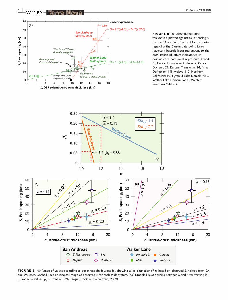
Figure 5 plots average fault spacing S against the seismogenic zone

thickness L for the San Andreas and Walker Lane fault systems.

Note that we present two data points for the Carson Domain: one

that includes S observations based on the three traditionally defined

Carson faults and one based on our reinterpretation of two addi-

tional faults (Figure 5). If we ignore the Carson data entirely, the

remaining three fault domains (i.e. Pyramid Lake, Walker Lake, and

the Mina Deflection) show a clear linear relationship (thick green

dashed line in Figure 5). The original three-fault Carson data point

plots significantly off this line, whereas the reinterpreted five-fault

data point plots in line with the other data (Figure 5). Based on

these observations and our preliminary geologic investigations, we

suggest that a five-fault Carson Domain better represents this sys-

tem within the Walker Lane. The following discussion assumes the

reinterpreted data point for the Carson Domain.

Both the San Andreas and Walker Lane fault systems show linear

S/L relationships (Figure 5). The S/L slope is steeper for the SA data

than for the WL system: ~8 vs. 1, respectively. The axis intercepts

for the two linear regressions differ significantly. The SA curve has a

negative vertical-axis intercept of S = 75 � 58 km, whereas the WL

curve has an S-axis intercept of 0 � 15 km (Figure 5). The ~9.7 km

horizontal-axis (L-axis) intercept for the SA curve predicts that for a

single fault strand in the SA system—such as the central San

Andreas fault—the seismogenic zone thickness at the fault should

be 9–10 km, which is supported by relocated seismicity (Lin et al.,

2007).

5 | DISCUSSION AND SUMMARY

To relate strike-slip fault observations to the stress-shadow model

(Equation 5), we assume L = h. However, L could overestimate h if L

actually consists of a frictional-sliding layer (hf) and a transitional

zone (hfv) of frictional sliding and viscous creeping (L = hf + hfv) (Fig-

ure 2). A diffuse brittle–ductile transition zone would, for a given

fault system, shift the S/L curve right compared with an S/h plot

because L ≥ h. The linear slope should not change. That said, the

WL S/L curve has a zero S-intercept (Figure 5). This suggests it was

not shifted by L overestimating h, or else the inferred S/h curve would

have a positive S-axis intercept, which is not observed in other

continental settings or analogue experiments (Zuza et al., 2017).

Given h�L, the S/h slope can constrain regional stress magnitude

(a) and the effective coefficient of fault friction (lf ) following our

stress-shadow model. However, we note that absolute solutions for

a and lf are highly sensitive to the chosen parameters, and therefore

we are most interested in relative differences between these values.

Rearranging Equation (5) and using the observed S/h slope for each

fault system, we plot a(lf ) (Figure 6a). In the Sierran and Western

Transverse blocks (i.e. areas without active parallel strike-slip faults)

H = 16–17 km (Zuza et al., 2017); thus a is ~1.6–1.2 and ~1.3–1.1

for WL and SA, respectively. We expect that the lowest a for each

fault system represents the effective remote stress driving stress-

shadow faulting. The estimated bulk friction coefficient for the SA

faults is lower (lf = 0.06) than for WL faults (lf = 0.19) (Figure 6a).

Alternatively, if a = 1.1 for both systems, lf is 0.06 and 0.22 for SA

and WL, respectively.

To examine possible ranges of a and lf , and demonstrate how

parameter variations affect the S/h slope, we plot S–h data against

modeled stress-shadow solutions using the above constraints as

parameter bounds (Figure 6b,c). First, we assume that an equal

regional shear stress is acting on both systems. The a proxy is an

upper bound, as originally defined, and we choose the lowest a

value common to both fault systems, a = ~1.15 (Figure 6b). This plot

shows that the SA faults (lf = 0.19–0.13) are relatively weaker than

those in the WL system (lf = 0.20). Alternatively, if we fix fault fric-

tion as a constant across all faults (i.e. lf = 0.18), we can explore the

relative difference in the a required to produce the observed S–h

relationship (Figure 6c). The a values overlap, although the SA a is

slightly lower than the WL a: 1.1 � 0.1 vs. ~1.2 respectively. Note

F IGURE 4 (a) Earthquake-location data for California used in this study from Schaff and Waldhauser (2005), Lin et al. (2007), Waldhauserand Schaff (2008), and Hauksson et al. (2012). Lines and letters represent the locations of earthquake-depth profiles plotted in (b–e). (b–e)Earthquake depth plotted as a function of horizontal distance across the Walker Lane fault domains. Profiles are oriented orthogonal to thestrike-slip faults in each domain. In each plot, the cutoff depth above which 95% (D95) of seismicity is contained in the crust was calculated.Dashed blue line represents the bulk average D95 depth, whereas the solid red lines represent the D95 depths in each segment of length l(dashed red line indicates larger l to accommodate remaining earthquake events that do not warrant an additional segment analysis)

4 | ZUZA AND CARLSON

0

5

10

15

20

25

30

0 20 40 60 80 100 120 140

Earth

quak

e de

pth

(km

)

Distance in the 50° direction (km)(b) Pyramid Lake

bulk D95

0

5

10

15

20

25

30

0 10 20 30 40 50 60 70 80 90

Earth

quak

e de

pth

(km

)

Distance in the 153° direction (km)(c) Carson Domain

D95 average: 10.5 ± 0.6 km

bulk D95

0 100 200 km

N

0

5

10

15

20

Depth (km)

40°N

118°W 116°W 114°W120°W122°W124°W

36°N

38°N

(d)(c)

(e)

(b)

0

5

10

15

20

25

30

0 20 40 60 80 100

Earth

quak

e de

pth

(km

)

Distance in the 69° direction (km)(d) Walker Lake

0

5

10

15

20

25

30

0 10 20 30 40 50 60 70 80

Earth

quak

e de

pth

(km

)

Distance in the 173° direction (km)(e) Mina Deflection

bulk D95

D95 average: 9.6 ± 1.9 km

D95 average: 11.2 ± 0.7 km

D95 average: 14.3 ± 1.4 km

bulk D95

(a)

ZUZA AND CARLSON | 5

Walker Lane fault system

S = 7.7(±4.5)L - 74.7(±57.6)San Andreas fault system

00

10

20

30

40

50

60

70

2 4 6 8 10 12L, D95 seismogenic zone thickness (km)

S, F

ault

spac

ing

(km

)

14 16 18

S = 1.1(±1.4)L - 0.4(±14.8)

“Traditional” Carson Domain datapoint

Reinterpreted Carson datapoint

Regression without Carson Domain

(a) r2 = 0.98

r2 = 0.86 Extrapolated L with single-fault strand

Linear regressions

C

WLM PL

MjET

NC

WSC

C’

F IGURE 5 (a) Seismogenic zonethickness L plotted against fault spacing Sfor the SA and WL. See text for discussionregarding the Carson data point. Linesrepresent best-fit linear regressions to thedata. Italicized letters indicate whichdomain each data point represents: C andC0 , Carson Domain and relocated CarsonDomain; ET, Eastern Transverse; M, MinaDeflection; Mj, Mojave; NC, NorthernCalifornia; PL, Pyramid Lake Domain; WL,Walker Lake Domain; WSC, WesternSouthern California

μ f= 0

.05

μ f= 0.10

μ f= 0.15

μ f= 0.20

μf = 0.23

α = 1.05

α=

1.01

α = 1.1α = 1.2

α = 1.4α = 1.3

(b) (c)

Mojave

E.Transverse

Northern

SWSan Andreas

Mina

Pyramid L.

Walker L.

CarsonWalker Lane

S, F

ault

spac

ing

(km

)

h, Brittle-crust thickness (km)0

0

10

20

30

40

50

60

4 8 12 16 20

S, F

ault

spac

ing,

(km

)

h, Brittle-crust thickness (km)0

0

10

20

30

40

50

60

4 8 12 16 20

0

0.05

0.10

0.15

0.20

0.25

α

α = 1.1, μf = 0.06

α = 1.2,μf = 0.19

1.0 1.2 1.4 1.6 1.8

μ f

Walker LaneSan Andreas

S/hWL: 1.1S/hSA: 7.7

α = 1.15

μf = 0.18

(a)

F IGURE 6 (a) Range of values according to our stress-shadow model, showing lf as a function of a, based on observed S/h slope from SAand WL data. Dashed lines encompass range of observed a for each fault system. (b,c) Modeled relationships between S and h for varying (b)lf and (c) a values. lu is fixed at 0.24 (Jaeger, Cook, & Zimmerman, 2009)

6 | ZUZA AND CARLSON

that the S/h curve of the WL faults has a near-zero S-intercept and

its slope parallels parameter contours, implying that the WL fault

domains have similar a and lf values, whereas the SA S/h curve

crosses parameter contours, suggesting that these values vary

between the fault domains (Figure 6b,c). Our overall low fault-fric-

tion estimates (0.2–0.1) (Figure 6) are consistent with previous stud-

ies (e.g. Bird & Kong, 1994; Fay & Humphreys, 2006).

The significant dissimilarities between the SA and WL S/L curves

(i.e. their intercepts and slopes) are probably related to different

mechanical properties of the strike-slip faults and the fault-hosting

crust. We envision several possibilities for how the local geology or

regional boundary conditions may affect the S–L relationships of a

given strike-slip fault system, including its slope and/or S- and L-axes

intercepts.

The steeper SA curve relative to WL may reflect lower fault fric-

tion because the fault-hosting crust in western California contains

friction-reducing clays and hydrated phyllosilicates (Collettini,

Niemeijer, Viti, & Marone, 2009) of forearc/m�elange materials (Dick-

inson, 1981) (Figure 7a). A lower effective shear stress may act on

the SA faults (Figure 7a). A lower strain rate ( _e) in WL predicts

lower �Y (Goetze & Evans, 1979) and therefore lower S/h slope (see

Equation 1). The negative y-intercept of the SA faults suggests that

the S/L curve, relative to WL, is translated right or down with a

thicker seismogenic zone L or smaller spacing S, respectively (Fig-

ure 7b). Apparent spacing decreases may be due to fault-healing

effects (Tenthorey & Cox, 2006) or abandonment of faults and acti-

vation of new ones as fault-bounded blocks rotate (Carlson, Pluhar,

Glen, & Farner, 2013), making certain previously active faults unfa-

vorable.

With higher strain, L in SA may be larger because the base of

the brittle crust developed asperities protruding into the underlying

viscous medium (Figure 7b); earthquakes would still occur in this

mixed frictional–viscous zone, increasing L (Pec et al., 2016). A

thicker L is also predicted by higher _e across the SA (Goetze &

Evans, 1979) (Figure 7b). Alternatively, the S/L curve difference may

be a result of higher heat flow for the WL in the Basin and Range

province (Blackwell et al., 2011; Bonner, Blackwell, & Herrin, 2003),

which would result in a thinner L. This would effectively shift the

S/L curve left without affecting its slope (Figure 7c).

The WL and SA strike-slip faults are earthquake hazards. Minimal

vertical offset and relatively slow slip rates on these faults have

made assessment of their slip histories and seismic risk problematic

(Wesnousky, Bormann, Kreemer, Hammond, & Brune, 2012). The

methods presented here of using S and L observations to evaluate

fault friction may help evaluate relative risk among strike-slip faults

(e.g. slip may be focused on faults with lower fault friction, or

greater elastic loading may occur on faults with higher friction). Fur-

thermore, estimates of fault characteristics can improve physics-

based models of the earthquake cycle and hazards (e.g. Console,

Carluccio, Papadimitriou, & Karakostas, 2015; Pagani et al., 2014;

Petersen et al., 2015).

Our strike-slip fault spacing investigation of the Walker Lane and

San Andreas systems reveals that both display linear S/L

relationships, but the SA curve has a steeper slope and negative S-

axis intercept. Assuming a stress-shadow mechanism, we explored

what these S/L curve differences mean for fault strength and regio-

nal shear stresses. This analysis suggests that fault friction of San

(a) Steeper S/L curve:

α↓: Lower effective regional stress acting on deforming domain

↑: Fault-bounded crust is stronger (colder and thicker?)

↓: Lower fault friction due to forearc/mélange phyllosilicates vs crystalline/sedimentary rocks

μf

μφ

L

S

(b) Negative y-intercept of S/L curve:

L

S

L = hf + hfv

hfv

hf

Larger transitional frictional/viscous zone (hfv) along higher straindeforming plate boundary

Frictional/seismogenic asperities in viscous medium

Decreased apparent S due to faulthealing and/or abandonment

L

S(c) S/L curve left could beshifted left because ofhigher geothermal gradient in Walker Lane(i.e., reduced L)

Original geothermal gradient

300 °C

500 °C

Perturbed geothermal gradient in Walker Lane

WalkerSanAndreas

300 °C

500 °C

Explanations for mechanical differences between the San Andreas and Walker Lane fault systems

↑: Increased yield strengthε

↑: Increased Lε

F IGURE 7 Models to explain the mechanical differencesbetween the San Andreas and Walker Lane fault systems, includingtheir different S/L curves (San Andreas: blue lines; Walker Lane:orange lines). (a) The steeper S/L SA curve may reflect the localgeology of the fault-bounding crust or different boundary conditions.(b) The negative S-axis intercept of the SA curve could suggest ashift in L or S relative to the WL fault system. (c) The elevated heatflow in WL may have decreased L, shifting the S/L curve toward azero S-intercept. Note that models are not to scale; see text fordiscussion

ZUZA AND CARLSON | 7

Andreas strike-slip faults may be lower than that of Walker Lane

faults. Variations in the local geology of the fault-hosting crust and/

or the regional boundary conditions may affect the observed

mechanical differences between the SA and WL fault systems, but

future research is needed to test our model constraints.

ACKNOWLEDGEMENTS

Startup funds at UNR supported this research. Comments from Alain

Tremblay, an anonymous reviewer, and Scientific Editor Jean Braun

greatly improved the presentation of our ideas in this manuscript.

REFERENCES

Atwater, T. (1970). Implications of plate tectonics for the Cenozoic tec-

tonic evolution of western North America. Geological Society of Amer-

ica Bulletin, 81, 3513–3536. https://doi.org/10.1130/0016-7606

(1970)81[3513:IOPTFT]2.0.CO;2

Bird, P., & Kong, X. (1994). Computer simulations of California tectonics

confirm very low strength of major faults. Geological Society of Amer-

ica Bulletin, 106, 159–174. https://doi.org/10.1130/0016-7606(1994)

106&lt;0159:CSOCTC&gt;2.3.CO;2

Blackwell, D., Richards, M., Frone, Z., Batir, J., Ruzo, A., Dingwall, R., &

Williams, M. (2011). Temperature at depth maps for the conterminous

US and geothermal resource estimates. GRC Transactions, 35, 1545–

1550.

Bonner, J. L., Blackwell, D. D., & Herrin, E. T. (2003). Thermal constraints

on earthquake depths in California. Bulletin of the Seismological

Society of America, 93, 2333–2354. https://doi.org/10.1785/012003

0041

Carlson, C. W., Pluhar, C. J., Glen, J. M., & Farner, M. J. (2013). Kinemat-

ics of the west-central Walker Lane: Spatially and temporally variable

rotations evident in the Late Miocene Stanislaus Group. Geosphere, 9,

1530–1551. https://doi.org/10.1130/GES00955.1

Carter, N. L., & Tsenn, M. C. (1987). Flow properties of continental litho-

sphere. Tectonophysics, 136, 27–63. https://doi.org/10.1016/0040-

1951(87)90333-7

Chiarabba, C., & De Gori, P. (2016). The seismogenic thickness in Italy:

Constraints on potential magnitude and seismic hazard. Terra Nova,

28, 402–408. https://doi.org/10.1111/ter.12233

Collettini, C., Niemeijer, A., Viti, C., & Marone, C. (2009). Fault zone fab-

ric and fault 206 weakness. Nature, 462, 907–910. https://doi.org/

10.1038/nature08585

Console, R., Carluccio, R., Papadimitriou, E., & Karakostas, V. (2015). Syn-

thetic earthquake catalogs simulating seismic activity in the Corinth

Gulf, Greece, fault system. Journal of Geophysical Research: Solid

Earth, 120, 326–343.

Davy, P., & Cobbold, P. R. (1988). Indentation tectonics in nature and

experiment. 1. Experiments scaled for gravity. Bulletin of the Geologi-

cal Institution of the University of Uppsala, 14, 129–141.

DeMets, C., Gordon, R., Stein, S., & Argus, D. (1987). A revised estimate

of Pacific-North America motion and implications for western North

America plate boundary zone tectonics. Geophysical Research Letters,

14, 911–914. https://doi.org/10.1029/GL014i009p00911

Dickinson, W. R. (1981). Plate tectonic evolution of the southern Cordil-

lera. Relations of tectonics to ore deposits in the southern Cordillera.

Arizona Geological Society Digest, 14, 113–135.

Dickinson, W. R. (1996). Kinematics of transrotational tectonism in the

California Transverse Ranges and its contribution to cumulative slip

along the San Andreas transform fault system. Geological Society of

America Special Paper, 305, 1–46.

Dokka, R. K., & Travis, C. J. (1990). Late Cenozoic strike-slip faulting in

the Mojave Desert, California. Tectonics, 9, 311–340. https://doi.org/

10.1029/TC009i002p00311

Dong, S., Ucarkus, G., Wesnousky, S. G., Maloney, J., Kent, G., Driscoll,

N., & Baskin, R. (2014). Strike-slip faulting along the Wassuk Range

of the northern Walker Lane, Nevada. Geosphere, 10, 40–48.

https://doi.org/10.1130/GES00912.1

Faulds, J. E., & Henry, C. D. (2008). Tectonic influences on the spatial

and temporal evolution of the Walker Lane: An incipient transform

fault along the evolving Pacific-North American plate boundary. Ari-

zona Geological Society Digest, 22, 437–470.

Faulds, J. E., Henry, C. D., & Hinz, N. H. (2005). Kinematics of the north-

ern Walker Lane: An incipient transform fault along the Pacific–North

American plate boundary. Geology, 33, 505–508. https://doi.org/10.

1130/G21274.1

Fay, N., & Humphreys, E. (2006). Dynamics of the Salton block: Absolute

fault strength and crust–mantle coupling in Southern California. Geol-

ogy, 34, 261–264. https://doi.org/10.1130/G22172.1

Goetze, C., & Evans, B. (1979). Stress and temperature in the bending

lithosphere as constrained by experimental rock mechanics. Geophysi-

cal Journal International, 59, 463–478. https://doi.org/10.1111/j.

1365-246X.1979.tb02567.x

Gold, R. D., Stephenson, W. J., Odum, J. K., Briggs, R. W., Crone, A. J., &

Angster, S. J. (2013). Concealed Quaternary strike-slip fault resolved

with airborne lidar and seismic reflection: The Grizzly Valley fault sys-

tem, northern Walker Lane, California. Journal of Geophysical

Research: Solid Earth, 118, 3753–3766.

Hauksson, E., Yang, W., & Shearer, P. M. (2012). Waveform relocated

earthquake catalog for southern California (1981 to June 2011). Bul-

letin of the Seismological Society of America, 102, 2239–2244.

https://doi.org/10.1785/0120120010

Jackson, J., McKenzie, D., Priestley, K., & Emmerson, B. (2008). New

views on the structure and rheology of the lithosphere. Journal of the

Geological Society, 165, 453–465. https://doi.org/10.1144/0016-

76492007-109

Jaeger, J. C., Cook, N. G., & Zimmerman, R., 2009. Fundamentals of Rock

Mechanics. 475 p.

Lachenbruch, A. H. (1961). Depth and spacing of tension cracks. Journal

of Geophysical Research, 66, 4273–4292. https://doi.org/10.1029/

JZ066i012p04273

Lin, G., Shearer, P. M., & Hauksson, E. (2007). Applying a three-dimen-

sional velocity model, waveform cross correlation, and cluster analysis

to locate southern California seismicity from 1981 to 2005. Journal

of Geophysical Research: Solid Earth, 112 (B12), 425.

Lister, G. S., & Davis, G. A. (1989). The origin of metamorphic core com-

plexes and detachment faults formed during Tertiary continental

extension in the northern Colorado River region, USA. Journal of

Structural Geology, 11, 65–94. https://doi.org/10.1016/0191-8141

(89)90036-9

Martel, S. J., & Pollard, D. D. (1989). Mechanics of slip and fracture along

small faults and simple strike-slip fault zones in granitic rock. Journal

of Geophysical Research, 94, 9417–9428. https://doi.org/10.1029/

JB094iB07p09417

Nagorsen-Rinke, S., Lee, J., & Calvert, A. (2013). Pliocene sinistral slip

across the Adobe Hills, eastern California–western Nevada: Kinemat-

ics of fault slip transfer across the Mina deflection. Geosphere, 9, 37–

53.

Nazareth, J. J., & Hauksson, E. (2004). The seismogenic thickness of the

southern California crust. Bulletin of the Seismological Society of Amer-

ica, 94, 940–960. https://doi.org/10.1785/0120020129

Pagani, M., Monelli, D., Weatherill, G., Danciu, L., Crowley, H., Silva, V.,

. . . Vigano, D. (2014). OpenQuake engine: An open hazard (and risk)

software for the global earthquake model. Seismological Research Let-

ters, 85, 692–702. https://doi.org/10.1785/0220130087

8 | ZUZA AND CARLSON

Pec, M., St€unitz, H., Heilbronner, R., & Drury, M. (2016). Semi-brittle flow

of granitoid fault rocks in experiments. Journal of Geophysical

Research: Solid Earth, 121 (3), 1677–1705.

Petersen, M. D., Moschetti, M. P., Powers, P. M., Mueller, C. S., Haller, K.

M., Frankel, A. D., . . . Olsen, A. H. (2015). The 2014 United States

national seismic hazard model. Earthquake Spectra, 31, S1–S30.

https://doi.org/10.1193/120814EQS210M

Pollard, D. D., & Segall, P. (1987). Theoretical displacements and stresses

near fractures in rock: With applications to faults, joints, veins, dikes,

and solution surfaces. Fracture Mechanics of Rocks, 277–349.

https://doi.org/10.1016/B978-0-12-066266-1.50013-2

Savage, J. C., & Lisowski, M. (1993). Inferred depth of creep on the Hay-

ward fault, central California. Journal of Geophysical Research: Solid

Earth, 98, 787–793. https://doi.org/10.1029/92JB01871

Schaff, D. P., & Waldhauser, F. (2005). Waveform cross-correlation-based

differential travel-time measurements at the Northern California Seis-

mic Network. Bulletin of the Seismological Society of America, 95,

2446–2461. https://doi.org/10.1785/0120040221

Segall, P., & Pollard, D. D. (1983). Nucleation and growth of strike slip

faults in granite. Journal of Geophysical Research: Solid Earth, 88, 555–

568. https://doi.org/10.1029/JB088iB01p00555

Stewart, J. H. (1988). Tectonics of the Walker Lane belt, western Great

Basin: Mesozoic and Cenozoic deformation in a zone of shear. In W.

G. Ernst (Ed.), Rubey Volume. Metamorphism and crustal evolution of

the western United States (pp. 681–713). Old Tappan, N.J.: Prentice-

Hall.

Stewart, J. H. (1999). Geologic Map of the Carson City 30 X 60 Minute

Quadrangle, Nevada. Reno, NV: Nevada Bureau of Mines and Geol-

ogy.

Tenthorey, E., & Cox, S. F. (2006). Cohesive strengthening of fault zones

during the inter-seismic period: An experimental study. Journal of

Geophysical Research, 111 (B9), 3051. https://doi.org/10.1016/j.epsl.

2016.09.041

Waldhauser, F., & Schaff, D. P. (2008). Large-scale relocation of two dec-

ades of Northern California seismicity using cross-correlation and

double-difference methods. Journal of Geophysical Research: Solid

Earth, 113 (B8), 501.

Wesnousky, S. G. (2005). The San Andreas and Walker Lane fault sys-

tems, western North America: Transpression, transtension, cumulative

slip and the structural evolution of a major transform plate boundary.

Journal of Structural Geology, 27, 1505–1512. https://doi.org/10.

1016/j.jsg.2005.01.015

Wesnousky, S. G., Bormann, J. M., Kreemer, C., Hammond, W. C., &

Brune, J. N. (2012). Neotectonics, geodesy, and seismic hazard in the

Northern Walker Lane of Western North America: Thirty kilometers

of crustal shear and no strike-slip? Earth and Planetary Science Letters,

329, 133–140. https://doi.org/10.1016/j.epsl.2012.02.018

Williams, C. F. (1996). Temperature and the seismic/aseismic transition:

Observations from the 1992 Landers earthquake. Geophysical Research

Letters, 23, 2029–2032. https://doi.org/10.1029/96GL02066

Yin, A., Zuza, A. V., & Pappalardo, R. T. (2016). Mechanics of evenly

spaced strike-slip faults and its implications for the formation of

tiger-stripe fractures on Saturn’s moon Enceladus. Icarus, 266, 204–

216. https://doi.org/10.1016/j.icarus.2015.10.027

Zuza, A. V., Yin, A., Lin, J., & Sun, M. (2017). Spacing and strength of

active continental strike-slip faults. Earth and Planetary Science Letters,

457, 49–62.

SUPPORTING INFORMATION

Additional Supporting Information may be found online in the sup-

porting information tab for this article.

Data S1 Discussion of fault domains in the Walker Lane.

Figure S1 Evenly spaced parallel strike-slip fault domains in the

Walker Lane. Fault data from Stewart (1999), Wesnousky (2005), Faulds

and Henry (2008), Wesnousky et al. (2012), and Gold et al. (2013). Note

that normal faults and smaller structures are omitted for clarity.

Figure S2 (a) Topography of the Carson Domain in the Walker Lane.

The three previously recognized northeast-trending structures are

shown (i.e. the Olinghouse fault, Carson lineament, and Wabuska linea-

ment) in addition to two previously undocumented parallel lineaments.

Also shown are the locations of Supporting Figures 2b–e. (b) Crop of

the geologic map of the Carson City 300 9 600 quadrangle (Stewart,

1999), which includes the southwestern part of the Carson Domain.

Dashed lines highlight lineaments and faults discussed in the text. Note

that the offsets and normal faults along the middle inferred fault are

consistent with left-slip kinematics. For individual unit descriptions,

please see the original Stewart (1999) reference. Also shown are loca-

tions of Supporting Figure 2c and the Google Earth image in Supporting

Figure 2f. (c) Unmodified zoom in on portion of Supporting Figure 2b

(map of Stewart, 1999) showing two left-lateral offsets of Tads unit (i.e.

interbedded Tertiary andesite and sedimentary rocks) consistent with

inference that Inferred Fault #2 is a left-lateral strike-slip fault. Also

shown are the locations of Supporting Figures 2d,e. (d–f) Remote sens-

ing analyses of the Inferred Fault #2 showing consistent ~300 m left-lat-

eral offset along its strike. Note that unit assignments are from Stewart

(1999). (d) ~310 m left-lateral offset of Tads-Tad contact. (e) ~305 m

left-lateral offset of Tba-Tads contact. (f) Topographic analysis of normal

fault-termination structure showing ~320 m horizontal motion, which is

kinematically compatible with similar magnitude left-lateral slip.

How to cite this article: Zuza AV, Carlson CW. What can

strike-slip fault spacing tell us about the plate boundary of

western North America?. Terra Nova. 2017;00:1–9.

https://doi.org/10.1111/ter.12315

ZUZA AND CARLSON | 9