west virgirda relevance for decisions
TRANSCRIPT

ED 062 709
AUTHORTITLE
PUB DATENOTE
EDRS PRICEDESCRIPTORS
IDENTIFIERS
ABSTRACT
DOCUMENT RESUME
EA 004 286
Johnson, Gary P.The Estimation of a Long Run Cost Function for WestVirginia Public High Schools.Apr 7240p.; Paper presented at Anerican EducationalResearch Association Annual Meeting (57th, Chicago,Illinois, April 3-7, 1972)
MF-$0.65 HC-$3.29*Costs; Decision Making; Educational Administration;*Educational Economics; *Expenditure Per Student;High Schools; *Input Output Analysis; Planning;Public School Systems; Resource Allocations; *School
Size; SpeechesWest Virgirda
This paper sets out a model that generates new,relevant information about the relationship among educational output,scale, and perpupil costs. According to the author, this information,if used, would result in more efficient educational spending.Specifically, a long run average cost function is estimated. Minimumperpupil operating costs are achieved when average daily attendanceis 1,426 students and the total square feet of the facility is124,062. Such a model has particular relevance for decisionspertaining to investment in new facilities and/or consolidation.(Author)

tU.S. DEPARTMENT OF HEALTH,
EDUCATION & WELFAREOFFICE OF EDUCATION
THIS DOCUMENT HAS BEEN REPRO-DUCED EXACTLY AS RECEIVED FROM
CPI THE PERSON OR ORGANIZATION ORIG-INATING IT. POINTS OF VIEW OR OPIN-
C:) IONS STATED DO NOT NECESSARILYREPRESENT OFFICIAL OFFICE OF WU-CATION POSITION OR POLICY.
ei)
CD
1:7.1 THE ESTIMATION OF A LONG RUN
COST FUNCTION FOR WEST
VIRGINIA PUBLIC HIGH SCHOOLS
A Paper Presented At
The 1972 Annual Meeting
of the
American Educational Research AssociatiOn.
by
Dr. Gary P. Johnson
The Division of Education Policy Studies
The Pennsylvania State University

One of the most important contributions ofeconomics to educational administration isa general concept of costs. Such a concept
has important implications for a conceptualapproach to decision-making. It is also a
valuable tool for the practicing administrator.1

Introduction: The Need To ConsiderAlternative Criteria In The Alloca-
tion Of Educational Resources
Public schools today face increasing financial pressure and what
appears to be a growing fiscal crisis resulting from certain endogenous
and exogenous changes. The most significant endogenous change has been
the relatively rapid rise of powerful teacher organizations which have
increased school operating costs considerably in recent years through
successful negotiations of higher teacher salaries and certain fringe bene-
fits. Exogenously, there exists presently a public preoccupation with vari-
ous notions of accountability, and an ongoing change in preference away from
public education to other goods and services as evidenced by the increasing
propensity towards non-support of public education.2
These changes have
placed increasing pressure on public education, in particular educational
administrators, to continue providing qualitatively similar educational
programs with relatively fewer resources and higher input prices.
This growing fiscal crisis has several ramifications, one of which is
particularly relevant here. Traditional criteria used by educational admin-
istrators in making expenditures and allocating resources may, out of immed-
iate necessity and/or long run conaiderations, need to be reordered, added
to, or poss ibly thrown out entirely and altogether new criteria established
(if we wish to maintain or improve the existing quality of educational
services presently being provided). More specifically, increasing system
needs relative to insufficient resources suggests changed administrative
behavior which emphasizes, for a given quality of educational output, ex-
pendtture criteria which reflect, to a greater extent than is presently the
'case, what I call 'enlightened efficiency factors.3

If new criteria are to be stablished or existing criteria reformulated
(resulting in greater efficiency in ducational spending which presently
appears appropriate), educational administrators must begin to identify and
stimate new and relevant information pertinent to this need. This paper
formulates and estimates a long run cost function for selected public high
schools in West Virginia. The cost function generates information potenti-
ally useful in decisions regarding new investment in high school facilities
and/or consolidation of existing ones. The information, if used, would
result in more efficient educational spending and a certain reduction in
system wide costs; thus providing educational administrators alternative
additional criteria information relevant to investment and consolidation
decisions. Specifically, the model indicates for the population being
sampled: (1) the relationship between per-pupil operating cost and educa-
tional output; (2) the optimum level of educational output (if one exists);
(3) the optimum size or scale of operations; (4) the scale of operations for
all output levels which minimizes per pupil costs; and (5) the extent of
economies of scale.
Theoretical Framework: The Short Run,The Long Run, The Relationship Between
Cost And Output, The Long Run CostFunction And Economies Of Scale
The Short Run And The bang_ Run
Theoretically, the analysis of cost is couched in one of two 'period
dimensions' -- either the short run or the long run. That is, the analysis
and conclusions regarding a firm1
s4
decisions and economic behavior will
differ significantly depending upon whether the firm is assumed to be opera-
ting in the short run or the long run. Understanding of the long run and
4

3
the short run and the relationship between the two becomes extremely import-
ant when one moves from the theoretical discussion of cost, cost functions
and economies of scale to the empirical estimation of cost functions from
real world date; therefore a discussion of both and the relationship betweEn
the two is included here.
Neither the short run nor the long run refer to calendar or clock time.
This is why they are often referred to as 'period dimensions', rather than
time periods. The two period dimensions, instead, refer to the time neces-
sary for individuals and firms to adapt fully to new conditions. For instance,
it cannot be said in advance and without reference to a specific problem or
situation that a one or two month period lies in the short run, or that a
ten year period extends into the long run.
Definitions of the short run and long run are ultimately concerned with
the degree of variability of different productive inputs. For a given period
of production, inputs are classified as either 'fixed' or 'variable'. A
fixed input is usually defined as one whose quantity cannot be easily or
readily changed (either increased or decreased) when conditions indicate a
change is either necessary or desirable. It is realized that no input is
ever fixed in the absolute sense, irregardless of how short the period of
time under consideration; but it is assumed that certain inputs can be
treated as constant or fixed, reasoning that the cost of inmediate variation
(either ars increasP or decrease) of these 'fixed' inputs is so large that
it places them well beyond consideration as a possible solution to the par-
ticular problem being considered. Such things as buildings, major pieces
of capital equipment and highly competent administrative personnel are
examples of inputs that cannot be rapidly increased.5
r-0

4
Thus a fixed input, while being necessary for production, does not change
with respect to changes in the quantity of output which is produced. A
'variable' input, on the other hand, is one which can be easily and readily
changed in response to desired or necessary changes in the level of output.
The fundamental difference then between fixed and variable inputs is
essentially temporal; in that inputs which are fixed for one period of time
are variable for a longer period of time. Thus, over a sufficiently long
period of time, all inputs are variable.6
Given the above distinction between fixed and variable inputs the short
run is defined as that period of time in which the amount or level of one
or more of the productive inputs is fixed.7
Two additional statements give
further insight into the theoretical-analytical construct of the short run:
..the short run is taken to be a period which is long enough topermit any desired change in output technologically possiblewithout altering the scale of plant, but which is not long enoughto permit of any adjustment of scale of plant.8
No variation in plant size will be made to adjust to fluxuationsin output in the short run...so there is no foregone alternativeto the more intensive use of plant. The only foregone alternative
is the amount spent on additional units of variable services (inputs).When we say that in the short run some inputs are freely variable,we mean that their quantity can be varied without affecting their
price (for a given quality). When we say that other inputs arenot freely variable, we mean that their quantities can be variedwithin the given time unit -- be it a month -- a week -- or a year-- only at a considerable change in their price....Fixidity and
variability are a matter of degree. In order to simplify theformal theory, economists define 'the short run' as a period within
which some inputs are variable, others fixed. Clearly there are
many short runs, and the number of freely variable productiveservices increases as the period of time is lengthened.9
Thus, the short run refers to a particular situation where at least one
of the inputs in the productive process is fixed; implying that increases in
5
output can only be achieved by either increasing the use of variable inputs
and/or utilizing the fixed input more intensively. No change in the scale
of plant is possible in the short run to achieve desired changes in output.
As an example of the short run, consider the situation where a particu-
lar school system is faced with a sizeable and unexpected increase in demand
for the educational services it provides. The only way the school system
can meet this increased demand (in the short run), if we consider existing
buildings as the fixed input and teachers as the variable input, is to uti-
lize both teachers and buildings more intensively and/or hire new teachers.
The school system in the short run cannot meet this increased demand by
increasing its scale of operations; that is, through construction of new
classrooms, gymnasiums or cafeterias.
In contrast, the long run refers to that period of time (or planning
horizon) in which all inputs are variable. It refers to that time in the
future when output changes can be achieved in the manner most advantageous
to the administrator.10
Elsewhere,11
the long run is defined as
a period long enough to permit each producer (administrator)to make such technologically possible changes in the scale of his
plant (facilities) as he desires, and thus to vary his outputeither by a more or less intensive utilization of existing plant,or by varying the scale of his plant or by some combination of
these methods.
Leftwich12
says of the long run:
The long run presents no definitional difficulties. It is a
period of time long enough for the firm to be able to vary thequantities per unit of time of all resources used. Thus, all
resources are variable. No problem of classifying resources asfixed or variable exists. The firm has sufficient time to varyits scale of plant as it desires from very small to large or vice
versa. Infinitesimal variations in size are usually possible.

Returning to our example of the school system faced with an unexpected
increase in client demand; the long run would be a period sufficiently long
to allow school administrators to respond to the increased demand for
educational services in virtually any manner they deemed appropriate (inclu-
ding Increasing the scale of operations). Thus, in the long run zero
constraints prevail.
The relationship between the long run and the short run. The relation-
ship between the long run and short run becomes crucial in determining the
estimation procedure used to arrive at a long run cost function for the
sampled population. It will become evident later that while analytically
and theoretically there exists a long run; in the real world, where data
must be collected, all production and all economic activity take place in
the short run.13
Thus, if we are (as in this case) attempting to emplri-
cally atimate theoretically postulated long run hypotheses and relationships
from real world cross-sectional data which is short run, an understanding
of the relationship between the two is absolutely essential. It is further
evident that if no relationship exists between the long run and short run,
empirical studies purporting to explain long run phenomena can have little
meaning if based on data reflecting short run economic activity.
Fortunately, there does exist a relationship between the long run and
the short run. Viewed slightly differently the long run refers to the fact
that administrators can plan ahead and choose any and as many aspects of the
short run they deem either necessary or appropriate. Thus, for a given
problem or situation, the long run consists of all possible short run
situations among which an administrator or economic agent may choose.14
This relationship allows one to move from the short run to the long run by
defining all possible short run situations for a particular problem. In our
6
-5

7
case it allows us to empirically estimate long run phenomena from data which,
in the real world, reflects short run activity.
The Relationship Between Cost And Output
In The Short Run
The cost curve or cost function expresses the relationship between cost
and output over some specified range of output for a given firm. Seven types
of costs are usually defined for the firm in the short run:
1. Total fixed cost quantity of the fixed productive input times its
price.
2. Total variable cost quantity of the variable productive input times
its price.
3. *Total cost total fixed cost plus total variable cost.
4. Marginal cost increase in total cost divided by the increase in
output.
5. Average fixed cost total fixed cost divided by output.
6. Average variable cost se total variable cost divided by output.
7. *Average cost average fixed cost plus average variable cost
total cost divided by output, or total cost (3.) divided by output.
The shapes of these various cost curves in the short run depend upon assump-
tions one makes about input prices and the production process. Specific short
run cost functions estimated from real world data may assume a variety of
shapes. One possibility which exhibits the properties15
usually assumed by
economists is given in Figures 1 and 2:16

0OUTPUT (Y)
Figure 1
8
8
0OUTPUT (Y)
Figure 2
The above set of short run cost curves depicts the relationship between
cost and output for a firs operating with one fixed input, usually assumed
to be the physical plant, or facilities in general. It is possible to define
and determine for each firm a specific set of short run cost curves such as
those depicted above; the actual or exact shape of the curves for each firm
being dependent on the particular output level and the size of the firm's
facility or plant.17
Thus, each time a firm increases or decreases the
size of its facilities (scale of operations), another set of cost curves will
need to be estimated or constructed if the relationship between cost and
output is to be accurately measured. In the short run then, a firm's cost
is a function of its output level and its scale of operations. This paper
is concerned specifically with those curves in the figures above labeled TC
and AC. These curves represent the firms' short run total cost and short
run average or perunit cost, respectively.
10

The Relationship Between Cost And OutputIn The Lot% Run
. .
In this section the long run average cost curve and long run total cost
curvet are discussed specifically. Also, the concept of economies of scale
in introduced and its role in determinfng the shapes of the long run average
and total cost curves is set out. Last, the notion of optimum scale of
operations (plant) is formally presented and briefly discussed. Throughout
this section two things discussed in previous sections should be remembered
or kept in mind: (1) the firm can choose and construct any desired scale
of plant in the long run, with all inputs becoming variable; and (2) the
long run can be viewed, with reference to a specific problem, as all possible
short run situations that the firm can choose to operate in.
The Long Run Averase Cost Curve.18
Let us assume for purposes of analy-
sis that it is possible for the school district to construct only 3 different
sized high schools. These are represented by SRAC1, SRAC2 and SRAC3 in
Figure 3 below. Each of the curves in Figure 3 represents the short run
average cos t curve for a particular and different sized high school (scale
of plant).
COST
Ct.
C4Cl
C. 3
5R,AC 1
RtipSRAC 3
'et
Figure 3
OUTPUT
it
9

10
In the long run the school disci-ict can construct any one of the three
different sized high schools. What sized high school should the district
construct? The answer depends upon the long run output which is to be
produced. Whatever the level of output is to be, the school district in
the long run will want to produce that level of output such that per unit
or per-pupil costs are minimal (for a given quality and quantity of educa-
tional services). Referring to Figure 3, assume output (or the flow of
educational services) is Y or projected to be at Y level per some unit of
time. The school district womld construct that sized high school represented
by SRAC1'
since it would result in a smaller per unit or per-pupil cost
(YC1) than will the other possible high school sizes. Per unit costs would
be YC2
if SRAC2were used. For output Y
1'the school district would be
indifferent between SRAC1and SRAC
2,(unless it expected substantial increa-
ses in output in the near future; in which ease, it would choose the scale
of plant indicated by SRAC2). For output Y2, it would construct SRAC2.
The long run average cost curve can now be defined: it gives the
minimum cost per unit of producing various outputs when the firm can construct
any desired scale of plant. Defined somewhat differently, the long run
average cost curve "is a locus of points representing the least unit cost
of producing the corresponding output.19 In the long run the broken seg-
ments of the SRAC curves become meaningless because the firm would never
operate on the broken segments since it could reduce costs by changing to
a different scale of plant.
The number of different sized high schools which a school district can
build in the long run are infinite. A series of SRAC curves representing
seven different possible high school sizes are depicted in Figure 4: Outer
11
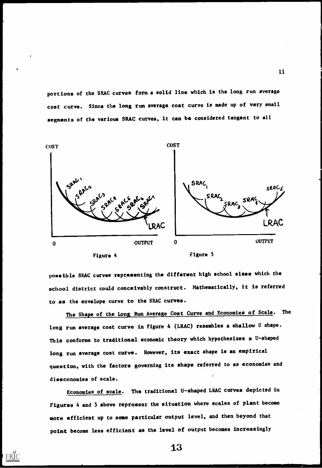
portions of the SRAC curves form a solid line which is the long run average
cost curve. Since the long run average cost curve is made up of very small
segments of the various SRAC curves, it can be considered tangent to all
COST
0
COST
SRAC,1
SRACIki4c
R Cs
4
seACs
LRAC
OUTPUT 0 OUTPUT
Figure 4 Figure 5
possible SRAC curves representing the different high school sizes which the
school district could conceivably construct. Mathematically, it is referred
to as the envelope curve to the SRAC curves.
The Shape of the Long_ Run Average Cost Curve and Economies of Scale. The
long run average cost curve in Figure 4 (LRAC) resembles a shallow V shape.
This conforms to traditional economic theory which hypothesizes a U-shaped
long run average cost curve. However, its exact shape is an empirical
question, with the factors governing its shape referred to as economies and
diseconomies of scale.
Economies of scale. The traditional U-shaped LRAC curves depicted in
Figures 4 and 5 above represent the situation where scales of plant become
more efficient up to some particular output level, and then beyond that
point become less efficient as the level of output becomes increasingly
13

12
larger. Increasing efficiency, associated with higher output levels and
larger scales of plant, is reflected by SRAC curves lying at successively
lower levels and farther to the right. This situation is depicted by SRAC/,
SRAC2and SRAC
3in Figure 5. Decreasing efficiency, associated with even
larger scales of plant, is depicted by SRAC4 and SRAC5 which lie at
successively higher levels and farther to the right. Thus, the U-shaped long
run average cost curve obtains.20
The forces causing the LRAC curve to decrease for larger outputs
and scales of plant are called economies of scale. Economies of scale can
be defined as net reductions in per unit costs resulting from long run
expansions in a firm's output.21 These net reductions in costs result from:
(1) increased specialization and division of labor; (2) greater proficiency
with increased concentration of effort; (3) reduction in excess capacity of
certain inputs; (4) many inputs becoming cheaper when purchased on a
larger scale; and (5) as the scale of operation expands there is usually a
qualitative change in equipment.
Diseconomies of Scale. The question arises why, once the scale of
plant is large enough to take advantage of all economies of scale, con-
tinued increases in output and scale eventually results in lesser efficiency
(the U-shaped LRAC curve). Theory suggests that limitations to the
efficiency of management in controlling and coordinating a single plant or
firm eventually occur.22 These limitations are called diseconomies of scale
and result from: (1) an overall breakdown in the coannunications network;
(2) the fact that administrators no longer receive the kind of information
necessary for optimum decision-making; (3) administrators must begin dele-
gating authority and responsibility to lower level and less competent
individuals; and (4) the organization becomes 'topheavy'.
14
13
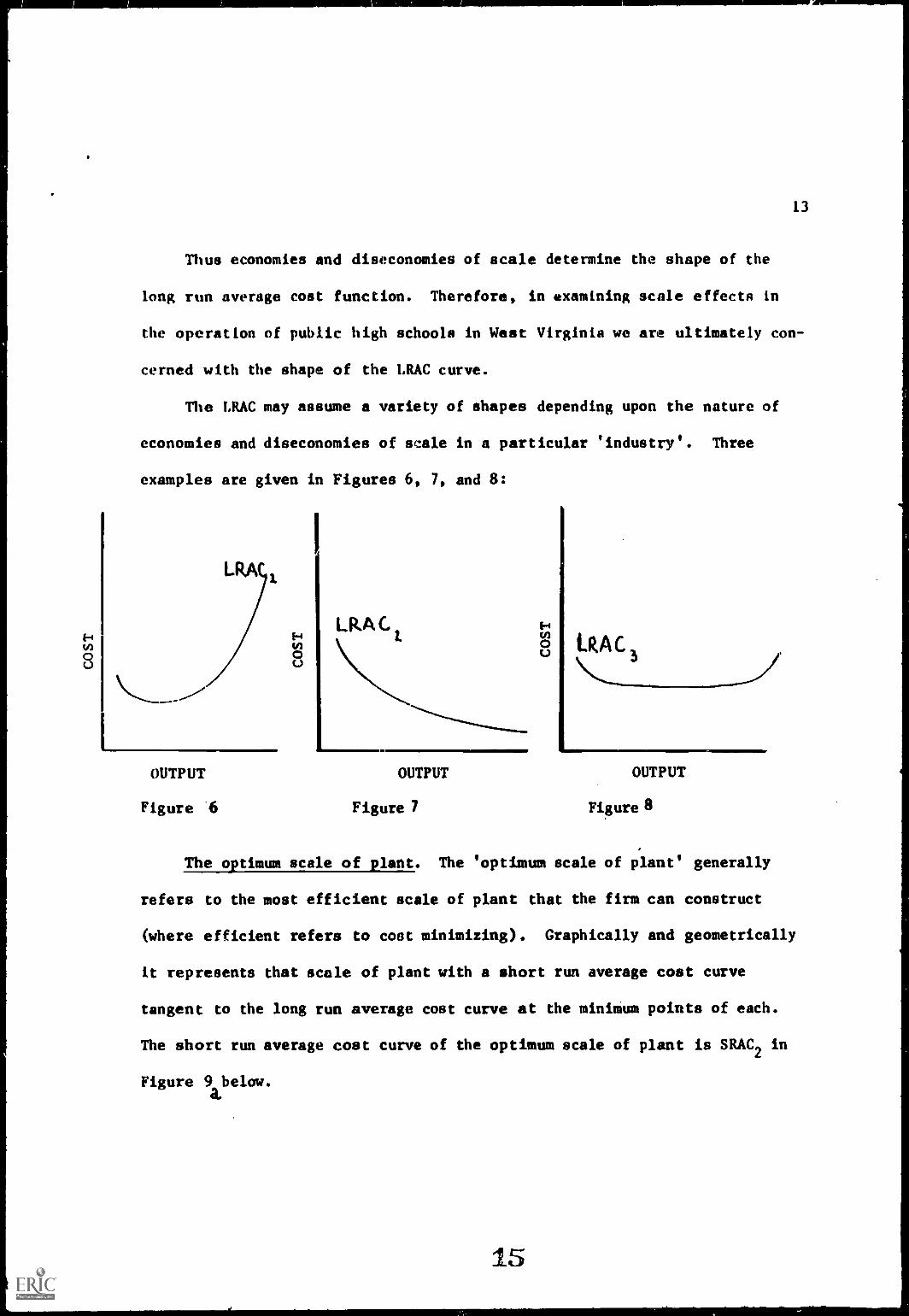
Thus economies and diseconomies of scale determine the shape of the
long run average cost function. Therefore, in examining scale effects in
the operation of public high schools in West Virginia we are ultimately con-
cerned with the shape of the LRAC curve.
The LRAC may assume a variety of shapes depending upon the nature of
economies and diseconomies of scale in a particular 'industry'. Three
examples are given in Figures 6, 7, and 8:
LRA
I-1
0C.)
LRA C
OUTPUT OUTPUT
Figure 6 Figure 7
,v)1"c:4, LIZAC
OUTPUT
Figure 8
The optimum scale of plant. The 'optimum scale of plant' generally
refers to the most efficient scale of plant that the firm can construct
(where efficient refers to cost minimizing). Graphically and geometrically
it represents that scale of plant with a short run average cost curve
tangent to the long run average cost curve at the miniium points of each.
The short run average cost curve of the optimum scale of plant is SRAC2 in
Figure 9 below.a.

COST COST
0 OUTPUT y
Figure 9a
o yFigure 10
vi
14
COST
0 yt
Figure 11
Yz OUTPUT
It should be noted that firms do not always construct the optimum scale
of plant, nor do they function at the optimum output level (except under
perfect competition). For example, in Figure 9 the scale of plant represented
by SRAC2 will produce output Y at a lower per unit cost than will any other
scale of plant, and output Y can be produced at a lower cost per unit than
can any other output. But for output levels greater or less than Y, per unit
costs will be higher. Scales of plant other than the optimum scale of plant
will produce these output levels at lower costs per unit than will the
optimum scale of plant. To prove this point, consider Figure 10. Suppose
the firm is producing output Y with the scale of plant SRAC1. The scale of
plant SRAC1
is being operated at less than its optimum rate of output. Assume
a change in output to Yl is contemplated. The increase in output can be
achieved in two ways: (1) by increasing the output with existing scale of
plant SRAC1, or (2) by increasing the scale of plant and moving to SRAC2.
16
15
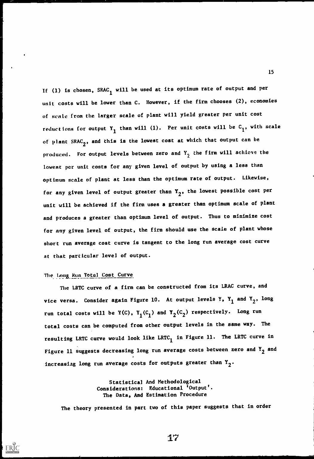
If (1) is chosen, SRAC1will be used at its optimum rate of output and per
unit costs will be lower than C. However, if the firm chooses (2), economies
of Neale from the larger scale of plant will yield greater per unit cost
reductions for output Yl than will (1). Per unit costs will be Cl, with scale
of plant SRAC2'
and this is the lowest cost at which that output can be
produced. For output levels between zero and Yl the firm will achieve the
lowest per unit costs for any given level of output by using a less than
optimum scale of plant at less than the optimum rate of output. Likewise,
for any given level of output greater than Y2, the lowest possible cost per
unit will be achieved if the firm uses a greater than optimum scale of plant
and produces a greater than optimum level of output. Thus to minimize cost
for any given level of output, the firm should use the scale of plant whose
short run average cost curve is tangent to the long run average cost curve
at that particular level of output.
The Lon Run Total Cost Curve
The LRTC curve of a firm can be constructed from its LRAC curve, and
vice versa. Consider again Figure 10. At output levels Y, Yi and Y2, long
run total costs will be Y(C), Y1(C1) and Y2(C2) respectively. Long run
total costs can be computed from other output levels in the same way. The
resulting LRTC curve would look like LRTC1 in Figure 11. The LRTC curve in
Figure 11 suggests decreasing long run average costs between zero and Y2 and
increasing long run average costs for outputs greater than Y2.
Statistical And Methodological
Considerations: Educational 'Output'.
The Data, And Estimation Procedure
The theory presented in part two of this paper suggests that in order
17

16
to determine the relationship between cost and output, and the extent to
which economics of scale exist in the operation of public high schools in
West Virginia, either a long run average cost curve or long run total cost
curve must be estimated. Before this is attempted, however, certain other
things should be discussed; specifically, the problem of 'educational output',
the data employed in the study and the method used to estimate the long run
cost function for selected public high schools in West Virginia.
Educational Output
For years, public school systems, researchers, academicians, interested
parents and government officials have been coucerned with 'educational output'.
Specifically, what is educational output, how can it be defined and measured?
Thus far no one has developed a universally accepted, additive and quantifi-
able measure which we can title 'educational output'.
Educators have set certain normative objectives such as the development
of individual potential, self expression, the fulfillment of individual
capacities and preparation of individuals for a democratic society.24
These
represent stated objectives. The difficulty of measuring, for a given
school, the extent to which any one of these goals is realized is immediately
evident.
The above represent only the stated objectives or manifest functions
of education. What about the measurement of the various latent functions25
which are supposedly performed by education? How can both the manifest and
latent functions be quantified, weighted and aggregated to obtain a measure
of 'educational output'?
The answer to this last question presupposes that we know what the
functions of public education are precisely. Some individuals such as Hills

suggest:26
17
...we do not know what the functions of education are.
Although there are volumes upon volumes of ideological exhorta-tions and prescriptions concerning what the functions of education
should be, there is relatively little in the way of concreteknowledge concerning the actual, objective consequences of exist-
ing educational activity. That is to say, we have a great deal
of information regarding the subjective dispositions -- aims,motives, and purposes -- attributed to education, but we knowlittle enough about what schools actually do, and practicallynothing about the objective consequence of these activities forthe larger structures in which the schools are involved.
Given the present state of knowledge regarding educational outputs and
the multiple output problem, several 'proxy' variables were considered and
one eventually chosen to represent educational output -- average daily
attendance.27 While not as glamorous as achievement test scores, it has
been used elsewhere28
as a proxy for educational output and is much less
restrictive and biased than achievement scores. The use of achievement
scores as a measure of educational output, a priori, limits educational out-
put to cognitive types, and is consistent with the narrowly defined normative
types of objectives and functions to which Hills refers. However, the
cognitive outputs may be only a very small part of the total educational
output.
In making average daily attendance a proxy for educational output, no
such restrictions on the nature of educational output apply; we are, instead,
stating simply, as average daily attendance increases so does the sum total
of educational experiences in the educational system. More precisely,
average daily attendance varies directly with educational output. Thus,
average daily attendance has at least two advantages within the context of
the above discussion: (1) as a measure of educational output it allows
educational output to include learning experiences beyond the cognitive
19
18
types; and (2) average daily attendance reflects indirectly both the mani-
fest and latent functions of the public school system more nearly than
other empirical measures thus far conceived.
Using average daily attendance as a proxy for educational output also
has a statistical advantage. Not only is average daily attendance relative-
ly stable and predictable over the academic year; but it is also highly
related to the total cost figure. Both these characteristics reduce potent-
ial bias in the estimation of the long run cost function.
A fourth consideration suggesting use of average daily attendance is
that in certain instances school boards, superintendents and other decision
makers use either average daily attendance or net enrollment (which is
highly correlated with average daily attendance) as a figure in various
types of decisions. The most obvious examples are the state aid formulas
and federal programs which base monetary allocations on either average
daily attendance or net enrollment. The underlying assumption is that some
minimum level of learning is occurring. Thus, in certain instances, average
daily attendance is treated as output or used as a basis for various admin-
istrative decisions.
The above considerations suggest several advantages in the use of
average daily attendance as a proxy for educational output. In light of
existing knowledge regarding the nature and functions of our educational
system, average daily attendance appears to be not only a reasonably 'good'
proxy for educational output but also an appropriate one.
The Data
There are fifty-five school districts in West Virginia. Forty-five
districts contain one or more senior high schools either grades nine to
r
20

19
twelve or ten to twelve. Data on cost and output were collected for the
1969-1970 fiscal year.
Senior high schools were chosen as the unit of analysis for essentially
two reasons: (1) school districts in West Virginia and other states are
(if they are not already there) moving away from the grade seven through
twelve concept; thus to estimate a long run cost function and investigate
the extent of economies of scale in senior high school operation is logically
most relevant and has potentially greatest benefit in terms of new informa-
tion for decision-makers; and (2) senior high school output or ADA is
flexible and can be considered a discretionary policy variable, in that
administrators at the district level have control over the various ADA
levels of senior high schools (i.e., through busing, consolidation and/or
investment in new facilities).
While there have been studies of scale effects at the district level,
these provide only marginally useful information to school administrators,
boards of education and state departments of education; because in many
states the school district is synonymous with the county, as is the case
in West Wzlinia. School administrators have no discretionary control
over district size. Changes in district or county size occur through
exogenous changes (i.e., industrial development or out migration). Thus,
to say the optimum sized school district is thirty-five thousand students
provides little relevant information to the board of education and district
superintendent simply because they have no internal control or mechanism
to effect district size.
Junior high schools and high schools grades seven to rwelve were
excluded from the study because of possible differences in organizational
structure which conceivably might confound estimation of scale effects and
-

20
make interpretation of results more difficult. Thus, the study involves
senior high schools grades nine through twelve and grades ten through twelve.
Data was gathered on high schools which ranged in average daily
attendance from 177 students to 21 30 students. Average daily attendance of
177 students represents the smallest output level while the average daily
attendance of 2130 students represents the largest output level actually
found in the state. Thus, the maximum possible range of output as measured
by ADA was obtained.
A total short run operating cost was obtained for each high school in
the sample for the 1969-1970 fiscal year. The figure represents an opera-
ting expenditure on administrative inputs, teacher inputs, instructional
inputs, operation and maintenance inputs. It accounts for no less than
ninety-seven percent of a school's current operating costs. The remaining
three percent include expenditures on such things as auxiliary services
(health programs, school lunches and other items). The figure is also net
of transportation costs which were impossible to calculate accurately on
a per school basis, bonded indebtedness and depreciation costs.
Qualitative differences and economies of scale. Interpretation of
studies examining economies of scale is extremely difficult if wide varia-
tions in school quality exist. For instance if per pupil operating expendi-
tures in school A are lower than in school B, but school B is qualitatively
superior to school A, little meaning can be attached to a discussion of
scale effects. Therefore, an attempt has been made here to minimize quali-
tative differences in schools to the greatest extent possible. The usual
procedure is to construct a school or district 'quality index' composed of
various school inputs and thereby 'control' for school quality either
explicitly or implicitly by introducing this index into the cost equation
22

21
or analysis. This procedure has been employed by several individuals in
examining public school expenditures and scale effects in public education.29
However, this procedure assumes, a priori, that the different inputs
used in the various indices relate to and measure school quality. Typical
input variables assumed to reflect school quality include: (1) the student-
teacher ratio, (2) per pupil expenditures, (3) number of books in school
library, (4) number of high school credit units offered, (5) percent of
teachers with master's degrees, (6) average teacher salary, (7) percent of
teschers in two or more fields.
Raymond30
in examining the relationship between selected input variables
and school quality concluded:
Empirical results pertaining to the state of West Virginia giveno support to the use of certain input variables as proxies forthe quality of education. There was no evidence of a significantrelationship between quality and student-teacher ratio, the percentof teachers in two or more fields, current expenditures, or theadequacy of library facilities. Thus, in spite of obvious andperhaps convincing arguments in support of theae factors, itappears that, in fact, they are mot always accurate indicators of
quality.31
Raymond did find, however, that salary variables were related to school
quality but warned at the same time against indiscriminant use of salaries
as a proxy for school quality. Referring to the above conclusions he says
of salaries:
No such unequivocal statement relating to teaching salariesmay be made. The significance of the salary variables providessome justification for the use of these variables as proxies forquality. On the other hand, it should be noted that the highestcoefficient of determination between a salary variable and aquality variable was about .36. This, in conjunction with thestrong relationships between salaries and population characteris-tics would seem to warrant only a very guarded use of salaries to
measure quality The exact nature of the relationship betweensalaries and quality could not be determined with available data.

22
Making limited use of these findings, all schooLswhose mean teacher
salary was $6250 or less were excluded from the population. It was felt
this procedure would reduce large variation in quality between schools.
Certain senior high schools had mean teacher salaries in the neighborhood
of $5500.
With the intent of further minimizing qualitative differences among
high ch9Als studied; a second procedure, used by Riew13
to minimize
qualitative differences among schools in a stu of economies of scale in
selected Wisconsin high schools, was also employed. Only those high schools
accredited by the North Central Association of Colleges and Secondary Schools
as of 1969-1970 were included in the population.
Establishing a minimum mean teacher salary and including only those
senior high schools which were North Centrally accredited reduced the
population size by thirteen observations. While all qualitative differences
are not eliminated by these two procedures, it is felt that enough variance
in school quality has been eliminated to make discussion of economies of
scale meaningful for the remaining senior high schools in the study.
From a population of sixty-five senior high schools in West Virginia
a purposive sample of thirty-eight observations was obtained. The sample
was purposive in two ways: (1) data was obtained so as to maximize the
range of observations on educational output in order to meet certain 'ideal'
data criteria for cost studies; and (2) because West Virginia has relatively
few schools whose average daily attendance exceeds twelve hundred students,
an attempt was made to obtain all observations of schools where ADA exceeded
one thousand students. The cost function estimated from this sample can be
considered representative of the population and descriptive of high schools
throughout the state in general.

23
We turn now to a discussion of the method used in estimating the
long run cost function for public high schools in West Virginia. In so
doing we answer the question why short run data was obtained to estimate the
long run cost function.
The Method Used In EstimatingThe Lons Run Cost Function
The method selected to estimate the long run cost function for public
high schools in West Virginia is suggested in Eads and Eads, Nerlove and
Raduchel.35 The procedure minimizes certain types of bias usually
associated with estimation of long run cost functions and is particularly
consistent with certain characteristics indigenous to public education; thus,
it provides an excellent procedure to estimate the long run cost function
here. The procedure makes use of the relationship between the long run
cost function and family of short run cost curves.
As indicated in part 2, the long run cost function gives the minimum
cost of producing each level of output under the assumption that the firm
is free to vary the size of its plant. However, as Eads, Nerlove and
Raduchel indicate, "except by chance, one never observes a firm on the
long run total cost function, but instead observes it on a short run
total cost function. The firm is unable in the short run to adjust all of
its factors of production to the optimum level for the output level it is
given to produce."36
As Henderson and Quandt37
suggest:
Long run total cost is a function of output level, given
the condition that each output level is produced in a plant
of optimum size. The long run cost curve is not something
apart from the short run cost curves. It is constructed from
points on the short run cost curves. Since size is assumed
'45

24
continuously variable, the long run cost curve has only one pointin common with each of the infinite number of short run cost
curves.Thus the long run cost curve is the envelope curve of the
short run cost curves, touching each short run cost curve and
intersecting none.38
It is this tangential relationship and the fact that most firms are
observed on their short run cost curve that suggests the procedure for
estimation of a long run cost function. Consider the production function:
f(X1, X2,. Xn) (3.1)
where Y represents output and X1, X2,...., Xn represent various inputs and
Xn
the fixed input (Plant or facility). The short run cost function
obtained from (3.1) under the assumption of cost minimizafion can be
written as:
C ) + p X(Y. Pr Xn n n
(3.2)
where pn are exogenously determined input prices. The above equation
states that total cost is a function of output level, input prices and plant
size. Writing this equation representing the family of short run cost
functions in implicit form we obtain:
C 0(Y, 17,19"Pn-1' Xn) - PnXn
6", Pn' Xn) °(3.3)
The condition existing at each point of tangency between a short run cost
function and the long run cost function is given by:
6 0aXn
(3.4)
Thus, solving (3.4) and substituting the result into (3.3) we obtain the
long fun cost function:
CL (Y, P1' .""Pn-1)
(3.5)
where long run cost becomes solely a function of output and the given
26

25
price of the inputs.39
The above discussion suggests an indirect method of estimating the
parameters of the unobservable long run cost function. One can estimate
the parameters of the family of short run cost functions and then make
use of this relationship between the short run cost functions and the
long run cost function to obtain the parameters of the long run cost
function.40
Consider the following example given by Henderson and Quandt41
. Assume
a short run total cost function of the following form has been estimated:
SRTC .04Y3- 0.9Y
2+ (11 - Xn)Y + 5X
2(3.6)
where Y represents output and X plant size or the fixed input. Now setting
the partial derivative of the implicit form of (3.6) with respect to Xn
equal to zero we obtain:
-Y + 10Xn
0 (3.7)
which has the solution Xn
.01Y. Substituting this result into (3.6) we
obtain the long run cost function:
SRTC 0.4Y3
- 0.9Y2+ 11 - .01Y(Y) + 5(0.1Y)
2
m .04Y3
- 0.95Y2+ 11!
Long run average cost is obtained from dividing LRTC by output (Y):
LRAC .04Y2- .095Y + 11.
The above model requires only that firms in the short run minimize costs;
that is, be somewhere on its short run average cost curve for a given level
of output and scale of plant.
This assumption appears to be extremely valid for public high schools
in West Virginia, because in most high schools, average daily attendance
has either remained relatively constant or even declined slightly since

1967. This relatively 'steady state' has allowed schools to make the
necessary adjustments which place them either on their short run cost
curve or the long run cost curve. Therefore, the procedure is utilized
here not only because it minimizes certain types of statistical bias but
also because the assumption of cost minimization appears consistent with
public high school operation in West Virginia.
To estimate the total cost function the procedure of ordinary least
squares was employed. It was chosen because it results in parameter
estimates which have certain desired properties. More precisely, least
squares estimators are best and unbiased. Further, least squares is most
appropriate where: (1) deviations between planned output and actual output
are small, (2) cross section data is employed and (3) the firm is only
concevned with cost minimization for given levels of output.42
All three
conditions set out above apply here and thus the method of ordinary least
squares was used.
Analysis, Findings And Conclusions
As suggested in section 2, we are most concerned with the shape of
the long run average cost function. It is the shape of the LRAC curve which
indicates the nature or extent of scale effects in a given 'industry'. The
shape of any curve is dictated by the particular mathematical function
specified. Thus, the question becomes what functional form best fits or
describes the data.
This is not always an easy question to answer for as Klein43
points
out, frequently in econometric research more than one hypothesis is con-
sistent with a given sample of data "and non-linear cost functions may
sometimes fit a given sample of data as well as a linear function."
28

27
Because the form of the function is crucial here the following method is
employed to avoid possible misspecification. First, a linear function
is estimated where cost CY) is a function of output (X). Then second and
third order terms in output (X2
and X3) are added and retained in the
1 1
regression equation only if their coefficients prove to be, on application
of the 't' test, significantly different from zero at the one percent
level. That is, we will only entertain the possibility of a curvilinear
total cost function if both the higher order terms differ significantly
from zero at the .01 level. Usually a measure of goodness of fit is
given by the R2 value. However, because both linear and non-linear
functions may give a good fit to the same data, the above procedure in
addition to examination of R2's is employed. Also the change in the mean
square will be examined upon introduction of the higher order terms.
Statistical Results
Total cost functions of the following general form were estimated:
Y1X1
+ bo + uA
3 A 2 0%Y b
3X1 + b
2X1+ bl X1 +Abo + u
(4.1)
(4.2)
where X1equals average daily attendance and Y equals total operating
cost. All total cost functions were forced through the origin.44
The
results are given in Table I below. When the additional higher order
terms are introduced into the equation, suggesting a curvilinear
relationship between cost and output, not only is the mean square reduced
by a significant extent but both regression coefficients of the higher
order terms are significantly different from zero at the .01 level. The
modest increase in the R2means little here because we are concerned with
the shape of the total cost function, in particular its departure from
29

TABLE I
RESULTS AND COMPARISON OF
EQUATION (4.1) AND
(4.2)
Equation
Number
A b1X1
A2
b2X
A3
b3X'
2R
Increase
in R2
F Value -
Total
Mean
Square
Mean Square
Reduction
(4.1)
(4.2)
Y =
509.47
(10.28)*
Y = 703.73X1
(51.53)*
-.37X2
(.08)*
.00015X3 1
(.00003)*
.9867
.9928
.9867
.0060
2453
1418
29414
17065
11349
Y = Total operating cost
X = Average daily attendance
*Indicates regression coefficient is significant at
the .01 level.
Figures in parentheses are the standard errors of
the regression coefficients.

29
linearity, which is suggested by the significant regression coefficients
of the higher order terms. It does appear, then, that the total cost
function is curvilinear and equation (4.2) is chosen here.
Consistent with the methodology previously set out, we now introduce
scale explicitly into the short run cost function estimated above. The
variable chosen to represent plant size was total square feet of high
school facility.45
Five short run total cost functions, each specifying
a different scale, output, and cost relationship, was estimated. The
rationale for this rather shot gun approach lies in the complexity of
second and third order models which yield 'surfaces'. As Draper and Smith46
indicate with regards to second and third order models, "omission of
terms implies possession of definite knowledge that certain types of
surface (those which cannot be represented without the omitted terms) cannot
possibly occur. Knowledge of this sort is not often available. When it is,
it would usually enable a more theoretically based study to be made." Of
the five equations specified and estimated, the following general form was
selected:
3 A 2 A 2Y b3X1 + b2X1 + bX
1+ c1X1X2 + C2X2 + u (4.3)
where Y equals total operating cost, X1 equals average daily attendance
and X2
equals total square feet of high school facility.
Estimation of the above generalized form resulted in the following
specific short run total cost function for selected public high schools
in West Virginia:
2 3SRTC 696.37X
1- .44672X
1+ .00013X
1
(59.52)* (.127)* (.00004)*
2+ .00174X
1X2
- .00001X2
(.00134) (.00001)
31
(4.4)
R2
.9934

Again, the regression coefficients of average daily attendance are significant
at the .01 level. The total F of the equation is 872.08. Also, inclusion
of the scale terms reduced the mean square from 17065 to 16641.
Following the procedures set out in section 3, the long run total cost
function for selected public high schools in West Virginia was obtained:
LRTCa
696.37X1
- .37103X2+ .00013X
3
1(4.5)
Dividing the above function through by X1 gives the long run average cost
function:
LRACa
696.37 - .37103X + .00013X2
1(4.6)
30
Given the empirically estimated long run average cost function for
selected high schools in West Virginia, is there some optimum scale of plant?
In section 2 the optimum scale of plant was given to be the most efficient
sized facility that could be constructed assuming variability of all inputs:
efficiency being synonymous with minimum cost for a given level of educational
quality. Graphically and geometrically it was said to be the scale of plant
resulting in a short run average cost curve whose minimum point also forms
the minimum point on the long run average cost curve. The question thus
becomes does the LRAC function estimated above have a minimum point or value?
The estimated long run average cost function for public high schools in
West Virginia was found to satisfy both the necessary and sufficient conditions
for a minimum value. Specifically, the minimum point on the long run average
cost function occurs where educational output, as measured by average daily
attendance, is 1426 pupils. That is, for a particular high school size when
average daily attendance is 1426 pupils, the cost per pupil in average daily
attendance will be minimum, or the lowest possible value.
To determine the specific scale which gives the tangency of both the
32

31
short run and long run cost curves at their minimum points we must
return to the estimated short run cost function. Performing certain opera-
tions the optimum scale of plant for the optimum output level of 1426 pupils
is found to be 124,062 square feet. At this point the short run and long
run and cost curves are tangent at the minimum point of both and long run
average cost or cost per pupil in average daily attendance will be minimum.
Having determined the optimum sized high school and optimum output level
let us now examine the actual shape of the LRAC curve over a relevant range
of educational output. The long run average cost curve depicted in Figure 12
represents the estimated LRACa function in (4.6). The curve has been drawn
for educational output ranging from one hundred students in average daily
attendance to three thousand students in average daily attendance. As indi-
cated previously, actual educational output for the population of sixty-five
schools ranged from 177 students in average daily attendance to 2,131 in
average daily attendance.
The shape of the long run average cost curve supports the maintained
hypothesis in economic theory of a U-shaped long run average cost curve.
It indicates that high schools will experience net economies of scale as they
increase their output and scale of operations from an average daily attendance
of 100 pupils up to 1426 pupils. Beyond this level of output, diseconomies
of scale outweigh economies of scale and long run average cost begins to rise.
Table II below gives an indication of the effect of scale on high
school operating cost. Specifically, it shows the change in long run average
cost resulting from equal incremental changes in output. We see that sub-
stantial economies of scale can be realized from increasing educational output
at the lower levels of output. Table II indicates that a high school which
increases its average daily attendance from one hundred students to three

AV
ER
AG
EC
OS
T (
i)
700
650
400
C.)
550
500
450
400 10
030
050
011
0014
2
ED
UC
AT
ION
AL
OU
TP
UT
(A0A
)
FIG
UR
E12
.

1
TABLE II
ME RELATIONSHIP BETWEEN SCALE ANDLONG RUN AVERAGE COST
ADA LRAC A LRAC
100 $661 $
300 597 -64
500 543 -54
700 500 -43
9 00 468 -32
1 100 446 -22
1 300 434 -12
1 500 432 - 2
1 700 441 + 9
1900 461 +20
2 100 491 +30
2 300 531 +40
2600 610 +79
2 900 713 103
r
Where: (1) LRAC equals total costdivided by pupils in averagedaily attendance
(2) t means change in
35
---
33
- -

34
hundred students can reduce its average cost per pupil by $64. Similarly,
substantial economies of scale are realized when the high school increases
its average daily attendance from 300 to 500 students. However, as output
and scale continue to increase reductions in long run average cost become
proportionately lesser. This suggests that economies of scale are becoming
exhausted and/or diseconomies of scale more prevalent. Finally, diseconomies
of scale become significant enough to outweigh economies of scale as output
and plant size continue to increase. Beyond this point, increases in output
and scale result in increased average cost.
It is interesting to note that virtually all high schools in the sample
could reduce per pupil operating costs by changing their scale of operations
and ADA levels; with over ninety percent of the sample being on the downward
sloping portion of the LRAC curve, the remainder being on the upward sloping
portion of the curve. Last, the model is capable of generating for any
given level of output, the optimum sized facility which would place the
school on zhe long run cost function.
36

FOOTNOTES
1 J. Alan Thomas, The Productive School: A Systems Analysis Approach toEducational Administration (New York: John Wiley & Sons, 1971), p. 31.
2. A number of factors support thin observation: (1) the increasing
percentage of school bond referendums which fail to obtain the necessarysupport; (2) district wide teacher layoffs which either go unquestionedby the public or are actually supported by them; (3) the reduction orelimination of extra-curricular programs, most noteably athletic andband programs; and (4) the current popularity of certain books whichare highly critical of education and its practices, processes, etc.
3. An 'enlightened efficiency' factor is any organizational variable, processor relationship which can be manipulated or changed (directly or indirec-tly) so as to produce a net reduction in operating cost, which leavesorganizational output qualitatively and quantitatively either unchangedor improved.
4. A firm is defined here as a technical unit or organization with institu-tional characteristics where commodities are produced. This definitionallows us to begin thinking of the high school as an 'educational firm'which utilizes a variety of productive inputs per academic year toproduce a certain flow of educational output.
5. C. E. Ferguson, Microeconomic Theory, (Homewood, Illinois: Richard D.
Irvin, 1966), pp. 107-108.
6. James A. Henderson and Richard E. Quandt, Microeconomic Theory: A
Mathematical Approach, (New York: McGraw Hill, 1958), pp. 42-43.
7. Ferguson, op. cit., pp. 107-108.
8. Jacob Viner, "Cost Curves and Supply Curves", A. E. A. Readings In PriceTheory, ed. Stigler and Boulding (Homewood, Illinois: Richard D. Irvin,
Inc., 1952), p. 202.
9. George J. Stigler, The Theory of Price (New York: Macmillan Company,
1966), pp. 134-135.
10. Ferguson, op. cit., p. 108.
11. Viner, op. cit., p. 205.
12. Richard H. Leftwich, The Price System And Resource Allocation, 3rd
ed.,
(New York: Holt, Rinehart and Winston, 1965), p. 130.
13. Ferguson, op. cit., p. 108.
14. Ibid., p. 176.
15. These cost curves depict a simplified situation, often assumed forpurposes of analysis, where: (1) the production process involves onlytwo inputs, one fixed and the other variable; (2) diminishing marginal
and average product eventually occur at some point for the variable
37

ii
factor; and (3) constant input prices are assumed. These assumptions
or conditions are consistent with the notion or definition of the
short run given earlier.
16. Henderson and Quandt, oz.._ cit., p. 56.
17. The size of the facility is usually referred to in economics as the
seal(' of operations. The two terms will he used interchangeablythroughout the remainder of the paper and can be considered synonymous.
18. Henceforth, our discussion wherever possible will be in terms of highschools rather than firms, and high school facility size rather thanfirms, and high school facility size rather than plant size. I considerit appropriate at this point to make a 'conceptual transformation' fromfirms to high schools and plant size to facility size. This will bring
the discussion closer to reality and also more readily indicate toeducational administrators the utility and applicability of theinformation obtained from the long run average cost function.
19. Ferguson, op. cit., p. 179.
20. Richard H. Leftwich, op. cit., pp. 143-144.
21. This definition 'of economies of scale is based on and essentially con-sistent with the definition given by Jacob Viner in "Cost Curves andSupply Curves," A. E. A. Reading!, In Price Theory, Volume VI, ed.
Stigler and Boulding (Homewood, Illinois: Richard D. Irvin, Inc., 1952),
p. 212.
22. Richard II. Leftwich, op. cit., p. 145.
23. Ibid., pp. 146-149.
24. John S. Brubacher, A History of The Problem of Education, (2" ed.;
New York:\ McGraw Hill, 1966), pp. 1-22.
25. The distinction between manifest and latent functions as a useful ana-lytical construct comes from Robert K. Merton, Social Theory And Social
Structure, (New York: The Free Press, 1968), pp. 73-138.
26. Jean Hills, "The Functions of Research For Educational Administration",Journal of Educational Administration, Volume 5, (No. 1, 1967), pp. 11-12.
27. ADA is obtained by dividing the total number of days all students haveattended by the total number of school days.
28. Elchanan Cohn, "Economies of Scale In Iowa High School Operations",Journal of Human Resources, Volume III, (No. 4, 1968).

4. iii
29. John Riew, "Economies of Scale in High School Operations," Review ofEconomics and Statistics (August, 1966), pp. 280-287; Finnis Welch,The Valuation of Human Capital" in Papers and Proceedings of theAmerica'', Economic Association, American Economic Review (May, 1966),pp. 379-392; Werner Z. Hirsch, ."BiTeWnants of Public Education Ex-penditures," National Tax Journal (March, 1960), pp. 29-40.
10. Richard Raymond, "Determinanta of the Quality of Primary and SecondaryPublic Education in West Virginia," Journal of Human Resources,Vol. 3,No. 4 (1968), pp. 450-470.
31. Richard Raymond, op. cit., p. 469.
32. Raymond, Ibid.
33. John Riew, op. cit., p. 281.
34. George C. Eads, "A Cost Function for the Local Service Airlines,"(Unpublished dissertation, Department of Economics, Yale University, 1968).
35. George Eads, Marc Nerlove, andFunction Vor the Local ServiceNon-Linear Estimation," ReviewNo. 3 (August, 1969).
William Raduchel, "A Long Run CostAirline Industry: An Experiment inof Economics and Statistics, Volume 51,
36. Ends, Nerlove and Raduchel, op. cit., p. 259.
37. Henderson and Quandt., op. cit., p. 60.
38. Ibid.
39. The above comes directly from Eads, et. al., 9.E. cit., p. 260 andparallels Henderson and Quandt, op. cit., p. 60.
40. Ibid.
41. Henderson and Quandt., op. cit., p. 61.
42. A detailed discussion of the use of least squares procedures inexamining and estimating cost-output relationships is given in J. Johnston,op. cit., pp. 30-43.
43. Lawrence Klein, An Introduction To Econometrics, (Englewood Cliffs:Prentice Hall, 1962), p. 121.
44. Initially, the total cost functions were estimated without being forcedthrough the origin. It eventually occurred to me, however, that a better
fit might be obtained if equations were forced through the origin becausethis seemed more consistent with the cost data collected. In this in-stance, intuition proved cor5ect. Forced equations resulted in a betterfit; evidenced by a higher R and significant increase in the total Fvalue.
39

l
1
45. This figure was obtained for each high school in the study fromthe West Virginia Rating Bureau, Charleston, West Virginia.
46. N. R. Draper and H. Smith, Applied Regression Analysis, (New York:
John Wiley and Sons, 1966), p. 130.