well test - boundary - 2 (week 09)
TRANSCRIPT

RESERVOIR BOUNDARIES
Azmi Mohd ArshadDepartment of Petroleum Engineering
Well Test InterpretationSKM4323

WEEK 09

CONSTANT PRESSURE BOUNDARY

Description
• A constant pressure boundary effect can be seen during a well test in several cases:– When the compressible zone reaches a gas cap laterally;
– When the compressible zone reaches an aquifer with the mobility of the water much greater than that of the oil


The Method of Images
• A constant pressure boundary is obtained analytically using the method of images.
• The image well is symmetrical to the tested well in relation to the boundary. – It has a flow rate opposite that of the tested well.

The Method of Images…/2

The Method of Images…/3
• Applying the image method, the pressure at the well is written:
)2r,(tpS)1,r,(tpp DDDDDDD −== (10.1)
Pressure variation due to
the well
Pressure variation due to the image
well

Distance to The Boundary
• Two methods can be used to determine the distance to the boundary:– The intersection of the semi‐log straight line and the constant pressure straight line that was reach at the end of the test.
– The radius of investigation at the time when the compressive zone reaches the boundary.

Distance to The Boundary…/2

Distance to The Boundary…/3
• Intersection of the two straight line:– The expression of the distance is identical to that obtained for a fault:
t
i
μckt012.0dφ
= (in practical US units) (10.7)

Distance to The Boundary…/4
• Radius of investigation:– The distance from the well to the boundary can be determined by the time tr when the measurement points leave the semi‐log straight line:
t
r
μckt032.0dφ
= (in practical US units) (10.8)

Type Curves: The Derivative
• The presence of a constant pressure boundary is characterized by a pressure stabilization.
• A pressure derivative going to zero and appearing as a sharp decrease of the log‐log representative corresponds to this pressure stabilization .

Type Curves: The Derivative…/2

Example 13
(In‐class workshop)‐ Constant pressure boundary‐

CLOSED RESERVOIR

Description
• If the reservoir is limited by no‐flow boundaries, two cases can be distinguished when the compressible zones reaches the limits:– The well is producing: when the no‐flow boundaries are reached, the flow regimes becomes pseudosteady‐state.
– The well is shut‐in: when the no‐flow boundaries are reached, the pressure stabilizes at a value called average pressure in the whole area defined by the no‐flow boundaries.

Pseudosteady‐State Regime• When all the no‐flow boundaries have been reached, the flow regime becomes pseudosteady‐state regime.
• The no‐flow boundaries define the drainage areaof the well.
*
234.0Ahmc
qB
tφ= (11.6)
Positive value

Pseudosteady‐State Regime…/2

Pseudosteady‐State Regime…/3• The value of P0 is used to determine the shape factor, CA.
⎥⎦⎤
⎢⎣⎡ −
−= m
PP h
mm 01
10456.5C *A(11.8)
From drawdown
From drawdown or buildup,
positive value

Pseudosteady‐State Regime…/4• Table 11.1 can be used to determine the tDAcorresponding to the end of the transient flow and to the beginning of pseudosteady‐state flow for a given reservoir‐well configuration:– The fourth column of the table indicates the exact beginning of the pseudosteady‐state flow;
– The fifth column shows the beginning of the pseudosteady‐state with less than 1% error;
– The sixth column gives the end of the transient flow with less than 1% error.


Pseudosteady‐State Regime…/11• Since pressure varies linearly versus time during the pseudosteady‐state flow, this flow is characterized on the pressure derivative by a straight line with a slope of 1 on a log‐log plot.
• The shape of the transition between the transient regime and the pseudosteady‐state regime dependson the shape of the drainage area on the position of the well in the area.- The shape of the transition is used to characterizethe reservoir well configuration.

Pseudosteady‐State Regime…/12

Pseudosteady‐State Regime…/13• Figures below shows a number of typical configurations and how they are characterized on the pressure derivative plot.
• It shows the boundary during a drawdown, but also during buildup (broken line).

Pseudosteady‐State Regime…/14

Pseudosteady‐State Regime…/15
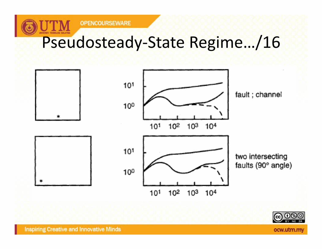
Pseudosteady‐State Regime…/16

Shut‐in Well, Average Pressure
• When the compressible zone reaches real no‐flow physical boundaries during buildup, the pressure in the drainage area becomes uniform and constant –average pressure of the drainage area.

Shut‐in Well, Average Pressure…/2
• A derivative going to zero corresponds to reaching the average pressure. It corresponds to a steep decrease of the derivative on a log‐log plot.

Shut‐in Well, Average Pressure…/3
• Comparison with a constant pressure boundary.

Shut‐in Well, Average Pressure…/4
• Calculating the average pressure using MBH (Mathews, Brons, Hazebroek) method:
Note: P* must be determined on the first semi-log straight line that corresponds to the infinite acting period

Shut‐in Well, Average Pressure…/5
1. Calculate tpDA :
2. Choose the curve corresponding to the reservoir-well configuration of the test (Figure 11.8 - 1.11).
3. Use the chart to determine:
4. Calculate the average pressure.
Ackt
t
p
μφ000264.0
tpDA =
( )m
pp −=
*
DMBH303.2P


Productivity Index• The productivity index of a well is the ratio between:
– The well flow rate;– The difference between the average pressure of the drainage area and the bottomhole pressure:
wfppq−
=PI (12.1)

Productivity Index…/2• Productivity index during the infinite‐acting period can be calculated by:
⎟⎟⎠
⎞⎜⎜⎝
⎛+−+
=S
rcktB
kh
wt
87.023.3loglog6.162PI
2φμμ
(12.2)
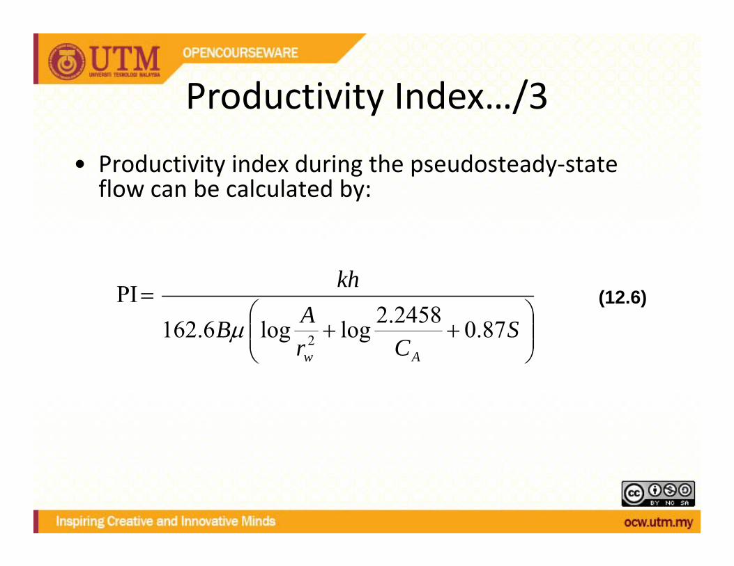
Productivity Index…/3• Productivity index during the pseudosteady‐stateflow can be calculated by:
⎟⎟⎠
⎞⎜⎜⎝
⎛++
=S
CrAB
kh
Aw
87.02458.2loglog6.162PI
2μ(12.6)

Example 14
(In‐class workshop)‐ Closed reservoir

References
1. Bourdarot, Gilles : Well Testing: Interpretation Methods, Éditions Technip, 1998.
2. Internet.