Economic Research Southern Africa (ERSA) is a research programme funded by the National

Treasury of South Africa. The views expressed are those of the author(s) and do not necessarily represent those of the funder, ERSA or the author’s affiliated

institution(s). ERSA shall not be liable to any person for inaccurate information or opinions contained herein.

Welfare and Environmental Impact of

Incentive Based Conservation: Evidence

from Kenyan Community Forest

Associations

Boscow Okumu and Edwin Muchapondwa

ERSA working paper 706

August 2017

Welfare and Environmental Impact of Incentive Based Conservation: Evidence from

Kenyan Community Forest Associations∗

Boscow Okumu†and Edwin Muchapondwa‡

Abstract

This paper focuses on whether the provision of landless forest-adjacent communities with options togrow appropriate food crops inside forest reserves during early stages of reforestation programmesenable vertical transition of low income households and conserves forests. We consider the welfareand environmental impact of a unique incentive scheme known as the Plantation Establishment andLivelihood Improvement Scheme (PELIS) in Kenya. PELIS was aimed at deepening communityparticipation in forestry, and improving the economic livelihoods of adjacent communities. Usingdata collected from 22 Community Forest Associations and 406 households, we evaluated themean impact of the scheme on forest cover and household welfare using matching methods andfurther assessed the heterogeneous impact of the scheme on household welfare using the endogenousquantile treatment effects model. The study revealed that on average, PELIS had a significantand positive impact on overall household welfare (estimated between 15.09% and 28.14%) and onthe environment (between 5.53% and 7.94%). However, in terms of welfare, the scheme cannot bedefended on equity grounds as it has inequitable distributional impacts on household welfare. Thescheme raises welfare of the least poor than the poorest and marginalizes sections of the communitythrough elite capture and lack of market linkages.

Key words: Household welfare, Heterogeneity, Selection, Matching, QTE

JEL Classification: D02, Q23, Q28

∗We are grateful to Environment for Development Initiative (EfD) and ECOCEP for financial support.†School of Economics, University of Cape Town; Private Bag Rondebosch 7701, Cape town. Corresponding author: kod-

his2000@gmail.com or okmbos002@myuct.ac.za.‡Professor, School of Economics, University of Cape Town. edwin.muchapondwa@uct.ac.za

1 Introduction

Conservation manifests itself today in various forms in different parts of the world. From statecontrolled such as reserve forests and exclusionary parks to community forests managed by lo-cal communities. Initial conservation efforts involved indigenous resource management based onsubsistence necessity, spiritual beliefs, experience, and traditions (Gbadegesin and Ayileka, 2000).Until the early 80s conservation efforts by governments in developing countries were mainly basedon the protectionist approach also referred to as the classic approach to conservation (Blaikie andJeanrenaud, 1997).

In developing countries, these forms of conservation have not yielded the best results in termsof conservation outcomes and welfare of local forest-adjacent communities. This is because indeveloping countries, natural forests are most often surrounded by high population of the poorbasically reliant on extraction of natural resources for their daily subsistence. Forest-adjacentcommunities are also often the poor without access to other sources of income such as land, humanand physical capital hence depend on income derived from the forests either directly or indirectly.Such dependence coupled with their high rate of time preference often leads to degradation of theresource thus contributing to further impoverishment of the dependent forest users. Hence, thepoor are considered to be agents and victims of environmental degradation as well (Wunder, 2001;Fisher, 2004).

The failure of the classic approach in many countries led policymakers and donors to concludethat the only solution is devolution of natural forest management to forest-adjacent communitiesthrough arrangements such as Participatory Forest Management (PFM) and provision of incen-tives in order to enhance community support, conserve forest and offer positive welfare benefitsamong the forest poor. Incentive based conservation has therefore been considered as a remedy tofailures associated with state control of natural resources such as, information asymmetry, incen-tive incompatibility or imperfect incentives, high monitoring and enforcement costs among others(Sterner, 2003; Adhikari, 2005). However, incentive based conservation has been marred with un-certainties since PFM places significant restrictions on extraction of forest resources. For example,in certain instances communities are required to pay user fees to access certain resources e.g., graz-ing, firewood collection etc. (Jumbe and Angelsen, 2006). Certain benefits are also restricted tomembership to CFAs. These practices have previously contributed to forest degradation in a way.Distributional problems have also been experienced with structured attempts at management ofCPRs (Kumar, 2002).

Attempts have therefore been made in support of incentive based conservation in a number ofdeveloping countries in recent years. In Kenya this attempt has focused on deepening communityparticipation in forest management to aid in conservation of forest and improvement of welfare offorest-adjacent communities through CFAs and incentive schemes. This is based on the premisethat other than devolution of forest management to local communities, provision of alternative

1

incentive to landless forest-adjacent communities may help them to avoid activities that may offershort term gains in favor of activities with long term payoffs. We consider one unique incentive inKenya known as Plantation Establishment and Livelihood Improvement Scheme (PELIS) underthe realm of PFM.

1.1 Incentive based Conservation in Kenya

Kenya’s forest cover of the land area stands at 7% far below the constitutional requirement of 10%.Approximately 80% of the Kenyan population reside in rural areas of which about 3 million livenext to forest hence relies either directly or indirectly on benefits derived from these forests. Theyalso directly rely on rain-fed subsistence agriculture for their livelihoods (FSK, 2006; WorldBank,2000). The five major Water Towers1 remains of significant importance to the economy since theysupply a range of ecosystem services such as water purification, biodiversity conservation, microclimate regulation, flood mitigation and hydrological services among others.

Improving forest governance has thus been an implicit objective in forest sector reforms in the lastdecade in Kenya (MENR, 2005, 2016). The Forest Act (2016) and Forest Act (2005) introducedPFM that seeks to engage local communities and promote private sector investment in gazettedforests. Some features of these Acts are: devolution of forest conservation and management throughPFM to local communities; introduction of benefit sharing arrangements such as PELIS; and adop-tion of ecosystem approach to management of forests among others. Communities have in turnbeen able to form community-based organizations (CBOs) known as Community Forest Associa-tions (CFAs) in collaboration with the Kenya Forest Service (KFS). This is a departure from priorpractice where the government fully managed gazetted forest reserves. In the Forest Act (2016),CFAs are recognized as partners in forest management and commercial plantations are also opento lease arrangements by interest groups to supplement conservation efforts. Apart from PELIS,there are various incentives2 aimed at encouraging forest-adjacent communities through CFAs tosustainably manage forests. To benefit from either incentives households are required to pay aspecific amount where a proportion goes to associated CBO or Forest User Group (FUG), CFA,and the highest proportion to KFS.

1.2 Motivation of the study

PELIS was first introduced in Kenya in 1910 by the colonial government as non-residential cul-tivation to promote livelihood of locals economically while ensuring sustainable management andconservation of forests through provision of raw materials for expanding timber industry and reducepressure on natural forests (Kagombe and Gitonga, 2005). Since forests in Kenya are surroundedby mostly poor households dependent on agriculture but constrained by inadequate agricultural

1Mau forest complex, Mt Elgon, Cherenganyi hills, Mt Kenya, and Abardare Ranges2These incentives include, bee-keeping, tree nursery, grazing, harvesting medicines and herbs, thinning (Silviculture) mainly for

fuel-wood, cutting grass for thatching, recreational activities, scientific studies, fish farming, eco-tourism and educational activities.

2

land and alternative sources of income, these scheme presents an opportunity for locals to derivelivelihood by planting appropriate food crops (Income from the sales of agricultural produce couldbe used to meet their daily household demands. There is also the nutritional value from consump-tion of these produce hence higher productivity due to improved health.) inside the forest reserveand also an incentive to conserve these forests as well3. Under the system farmers are allowed togrow both plantation trees4 and food crops on small plots (half an acre) tending the trees andharvesting crops for 3-4 years until tree canopy closes an arrangement where both parties benefit.It was later banned after several attempts in 1986, 1994, and 2003 due to failure and mismanage-ment. The scheme was however reintroduced in 2007 with enactment of Forest Act (2005) throughCFAs. Members are required to pay between Ksh. 400(4USD) and Ksh.750(7.5USD) per half anacre. The rules of allocation of plots also varies, with almost all CFAs purporting to use balloting.But this is just on paper as the process is marred with a lot of irregularities5.

However, even though PELIS may enhance efficiency in forest resource use, there may be in-equitable distribution of the benefits across the income groups hence a recipe for tragedy. It istherefore inherent to gauge PELIS impact not just with reference to its efficiency and effectivenessbut also by sustainability of the benefits in promoting equity and improvement of environment.There is also limited understanding of the drivers of adoption of the scheme by households withinCFAs which could shed light on reasons for past failures in the scheme and identify possible factorsto consider in rolling out the scheme. In addition, since the opportunity cost of restriction of forestaccess and use is higher among the poor, there is uncertainty whether participation in PELIS canenable poor households move up the income ladder. There is also high likelihood of those highup the ladder capturing the scheme hence having a disproportionate impact on the distribution ofprogram benefits. Empirical evidence on the impact of PELIS on environmental conservation andwelfare implication is also not clear despite its significance for sustainability of PFM.

Moreover, studies that have analyzed various forms of forest management activities are more biasedtowards Asia mostly Nepal and India. There are relatively few studies in Africa (see Jumbe andAngelsen 2006; Kabubo-Mariara 2013; Gelo and Koch 2014; Mazunda and Shively 2015; Geloet al. 2016). Empirical studies that have tried to evaluate the welfare effects of various incentiveshave mainly been focused on mean impacts assuming constant treatment effects across the incomedistribution (see Gelo and Koch, 2014; Ali et al., 2015; Mazunda and Shively, 2015), with veryfew on the heterogeneous impacts of such schemes (see Adhikari, 2005; Jumbe and Angelsen,2006; Cooper, 2007, 2008; Moktan et al., 2016; Gelo et al., 2016). A general overview of thesestudies reveals significant differences in applied definition, contextual factors and methodological

3Once one becomes a participant in PELIS, the benefits will depend on, one’s hard work and the kind of crops grown as well as, howwell they market their produce to fetch better prices.

4Farmers are usually provided with tree seedlings by the KFS and each is tasked with nurturing the trees planted in their plots.In case any tree gets destroyed one is answerable to the CFA officials and the forester. In certain instances, a penalty is applied. Inaddition, CFAs may also construct their own nurseries in the forest and sell tree seedlings to members for setting up their privatewoodlots.

5During the survey, we noted that some CFA officials and members had more than one plot in the forest while some deservingmembers had none. Some rich established non-members also acquired plots in the forest by bribing the foresters or CFA officials. Somemembers therefore felt short changed because only the well-connected members or elites tend to get the plots. Hence an incentive forthem to just sit back and watch as the forest gets destroyed.

3

approaches (ranging from, treatment effects models, PSM to instrumental variable) hence makingcomparison difficult. The results have also been mixed and inconclusive. On the other hand, themeasurement of outcomes employed in these studies are also significantly different hence prone tomeasurement errors. For instance, some studies use household income which is prone to underreporting especially among poor rural communities. As a departure from past studies that havealways classified households in terms of low, middle and high income households, and given thefact that measures of mean impact may not provide a clear picture of the impact of the scheme,we estimate the heterogeneous impact across the entire income distribution. The overall impacton forest cover and household welfare, and the heterogeneous impact of the scheme on householdwelfare therefore, motivates this study. The study therefore, seeks to fill these gaps by addressingthe following research questions: What determines households’ decision to participate in PELIS?What is the joint overall impact of PELIS on forest cover and household welfare? What is thedistributional impact of PELIS on welfare of locals?

This study contributes to the growing body of literature on impact evaluation of environmentalpolicies by providing a comprehensive empirical evidence from a micro perspective of the heteroge-neous impact of PELIS on household welfare and its simultaneous overall effect on the environmentand household welfare. From a policy perspective, an understanding of the overall and distribu-tional impact of the scheme across the income distribution has the potential to inform design,implementation and roll out of PELIS to other CFAs. Lessons from this scheme can also be usedto inform formulation of other market based incentives that can help in optimizing welfare gainsand improving environmental conditions. The rest of the paper is organized as follows: Section 2presents a description of the study area; section 3 outlines the methodological framework; section4 presents the survey design and data collection; section 5 presents the results and discussions;conclusion and policy recommendations are presented in section 6.

2 Description of the study area

The study was conducted in the Mau forest conservancy. The choice of Mau forest was based on aset of criteria namely, high susceptibility to degradation, long history of community forestry andhigh level of biodiversity. It is also the largest closed canopy forest among the five major WaterTowers in Kenya that has lost over a quarter of its forest resources in the last decade (Force,2009). It is located at 0°30’ South, 35°20’ East within the Rift Valley Province. It originallycovered 452,007 ha but after the 2001 forest excisions the current estimated size is about 416,542 ha. The Mau forest conservancy also has the highest number of CFAs with long history ofcommunity participation in PELIS. The Mau comprises 22 forest blocks, of which 21 are gazettedand managed by KFS. The remainder is Mau Trust Land Forest (46, 278 ha) which is managedby the Narok County Council (NEMA, 2013). The Mau ecosystem is the upper catchment ofmany major rivers. These rivers feed into various lakes e.g., Nakuru, Baringo, Natron, Naivasha,

4

Turkana, and Victoria. The lakes and rivers also provide water for pastoral communities andagricultural activity and supply essential ecosystem services. In addition, the estimated potentialhydro-power generation in the Mau forest catchment is approximately 535 MW, which account for47 percent of the total installed electricity generation capacity in Kenya UNEP (2008). The uppercatchment of the forest also hosts the last group of hunter gatherer communities such as the Ogiek(Force, 2009).

3 Methodological Framework

The framework is grounded in Roy (1951) occupational choice model. We assume that householdsdecide whether to participate in PELIS or not based on option that maximizes their utility. Ifhouseholds expect to benefit from participating in the scheme, then we assume they will join thescheme. Treatment assignment is therefore non-random. In particular, we define Vij the utility ofhousehold i =1...N in treatment regime j={0,1}, with 1 representing participation in PELIS and0 otherwise. Therefore, Di=1 if Vi1 > Vi0. Similarly define Yij as a vector of potential outcomevariable. Where Yi1is per capita expenditure and forest cover for PELIS beneficiary householdsand CFAs respectively andYi0 is per capita expenditure and percentage forest cover for non PELISbeneficiaries. The difference between Yi1and Yi0 can therefore be used to measure the differentialimpact on forest cover and household welfare.

In this study, we measure success in terms of household outcome and community level outcome thatis per capita expenditure and forest cover respectively and measurement depends on counterfactual.According to Rubin (1973), we define program impact as the difference between the observed andthe counterfactual outcome. The challenge is that the counterfactual is not observable and anindividual or CFA cannot be in both states at the same time. To identify the counterfactual,we apply a quasi-experimental approach given that participation in PELIS is non-random. It istherefore essential to control for participation decision to identify the impact of the scheme. Toexamine the impact of this incentive, the study takes account of the fact that differences in percapita expenditure or forest cover for participant households or CFAs and non-participants could bedue to unobserved heterogeneity. Failure to distinguish between the causal effects of participationin PELIS and effect of unobserved heterogeneity may therefore lead to misleading conclusion andpolicy implication.

PELIS has two possible levels of selection. In one level, households are deemed to be eligibleonly if they are members of CFAs and actively involved in CFA activities6. In another leveleligible households are left to decide whether they want to participate in PELIS7 by participatingin a balloting exercise or first come first serve basis in some instances. Households are likely toparticipate if they expect the potential gains to exceed the costs. In addition, Poor households

6In some CFAs there are also non-members who have PELIS plots we consider these as contamination and avoid them in the study.7However, based on their interest, they can decide to join other forest user groups for example bee keeping, tree nursery, grazing or

firewood collection groups.

5

may be eligible but unable to raise the fee whereas richer households may capture the schemeand obtain more plots at the expense of active eligible but poor households. On the other hand,richer households may find the opportunity costs of participating in the scheme to be higher hencemay consider other alternatives. Participation in PELIS is also potentially endogenous to percapita monthly expenditure. Some unobservable characteristics that influence the participationin PELIS could also influence per capita monthly expenditure e.g. household income or access toinformation. Therefore, neglecting these selectivity effects is likely to give a false picture of therelative per capita monthly expenditure for beneficiaries and non-beneficiaries of PELIS. Hencethe estimated causal effect may reflect not only the treatment effect but also differences generatedby the selection process.

On the other hand, the decision as to which CFAs get to benefit from PELIS is solely at thediscretion of KFS. The study therefore adopts a combination of econometric methods namely; thePSM and ordinary least square regression to determine the average treatment effect of participationin PELIS on per capita monthly expenditure and forest cover. However, OLS and PSM would yieldbiased estimates if there are unobservable determinants of participation. Control function methodsor Instrumental Variable methods becomes essential in such instances (see Wooldridge, 2010). Inaddition, since PSM and OLS models focuses more on the mean outcomes, we employed theQTE model under endogenous assumption following Abadie et al. (2002) to implicitly explore thedistributional impact of the scheme on household welfare while addressing the potential endogeneityto assess the sustainability of the scheme.

3.1 Propensity Score Matching

3.1.1 Theoretical and analytical framework.

The theoretical foundations follow Roy (1951) and Rubin (1974). Accordingly, households’ orCFAs’ decision to participate in PELIS is assumed to depend on expected benefits, as measuredby per capita expenditure and forest cover (The better the forest cover the more the benefits)in adjacent forest resource, associated with either participating in the scheme or maintaining thestatus quo. The main interest is the average treatment effect on the treated (ATT). That is howbenefiting from PELIS affect conservation and welfare of forest-adjacent communities. Since itis not possible to observe what the results would have been in the absence of the incentive. Tohandle the missing data on counterfactual, we identified households, which are non-beneficiaries ofthe incentives and used them as counterfactual. Similarly, for forest cover we identified CFAs thatwere non beneficiaries of PELIS and used them as counterfactual. Since assignment to PELIS isnon-random there is high possibility of selection bias. To address these issues, we first employedthe PSM technique to measure the mean impact on both forest cover and household welfare.

6

Identification strategy

Assuming a set of observable covariates X, which are unaffected by the treatment (Participationin PELIS), potential outcomes are independent of treatment assignment i.e., Conditional Indepen-dence Assumption (CIA)8. A further requirement is a sizable common support or overlap condition.This rule out the phenomenon of perfect predictability of T given X:

(Overlap) : 0 < P (T = 1|X) < 1 (1)

This condition ensures that households with the same X values have positive probability of beingboth participants and non-participants (Heckman et al., 1999). The effectiveness of PSM alsodepends on having a substantial region of common support or overlap (Khandker et al., 2009). Forestimation of the ATT, the assumption can be relaxed to P (T=1 X ) <1.

If the CIA holds and there is sizable overlap (Heckman et al., 1999), then the next step is to findthe PSM estimator. PSM was undertaken in two steps. The first step was generation of propen-sity scores from probit model using the household socio-economic and demographic characteristics,community level characteristics and other controls. The score indicates the probabilities of respec-tive households/CFAs participating in the scheme. From the scores, we constructed a controlgroup by matching the beneficiaries to non-beneficiaries according to their propensity scores bycomparing various methods of matching. The second stage involved computation of the ATT ofhouseholds and CFAs benefiting from incentives on household welfare and forest cover respectivelyusing the matched observations.

3.1.2 Model specification

The PSM estimator for the ATT is specified as the mean difference in Y (per capita householdexpenditure and forest cover as a percentage of total forest area under each CFA) over commonsupport, weighting the comparison units by the propensity score distribution of participants. Thecross section estimator is specified as:

τPSMATT = E(P (X)|T = 1){E[Y (1)|T = 1, P (X)]− E[Y (0)|T = 0, P (X)]} (2)

Where Y (1) and Y (0) represents per capita household expenditure and forest cover for beneficiaryand non-beneficiary households/CFAs respectively. T=1 indicates treated/beneficiary householdsor CFAs while T=0 indicates control/non-beneficiary households or CFAs. The PSM estimator isthus given by the mean difference in outcomes over the common support weighted by the propensity

8This assumption is rather strong and needs to be justified by the data quality at hand.

7

score distribution of participants9 (Caliendo and Kopeinig, 2008). To determine the heterogeneouseffect of the scheme on household welfare, and due to the restrictive identification condition,selection issues and potential endogeneity, the study also employed the use of the conditional QTEmodel under endogenous assumption described in the next section.

3.2 Quantile Treatment Effects Model

Measures of mean impact may not provide the true picture of the effect of the scheme, it istherefore essential to determine the heterogenous impact of the scheme to assess the sustainabilityof the scheme in providing the double dividend10. To determine the distributional impact of thescheme on household welfare, the study employed the parametric conditional QTE model underendogenous assumption following Abadie et al. (2002) and Chernozhukov and Hansen (2008).

3.2.1 Conceptual Framework

Given a continuous outcome variable Y, we consider the effect of a binary treatment variable D(participation in PELIS or not). Let Y 1

i and Y 0i be the potential outcomes of household i that is per

capita monthly expenditure. Hence, Y 1i would be realized if household i participated in PELIS and

Y 0i would be realized otherwise. Define Yi as the observed outcome, which is Yi = Y 1

i Di+Y0i (1−Di).

We estimate the entire distribution functions of Y 1 and Y 0 (Frölich and Melly, 2010).

We then define QTE conditionally on covariates as we deal with the endogenous treatment choicesince in our case, selection is unobservable meaning that treatment assignment is non ignorable.Participation in PELIS is also potentially endogenous to per capita expenditure11. The traditionalquantile regression may therefore be biased hence the need for an instrumental variable (IV) torecover the true effects. Key concerns with respect to instrumental variables are, weak instru-ments and over identification12. In addition, if the instruments affect participants in different waysinterpreting the resulting treatment effects may be complicated that is treatment effects hetero-geneity (Frölich and Melly, 2010). The exclusion restriction is however difficult to test as in all IVapplications.

Assuming we observe a binary instrument Z, we define two potential treatments denoted Dz.We then make use of several assumptions13 underlying the potential outcome framework for IVwith probability one as in Abadie et al. (2002). In addition to these assumptions, “individuals

9According to Caliendo and Kopeinig (2008), inclusion of non-significant variables cannot lead to inconsistent or biased results. Wethus used all the variables in the PSM probit in the outcome analysis.

10That is, improving household welfare and forest conservation and management.11Participation in PELIS is mostly influenced by household income which also directly influences per capita expenditure for both

participants and non-participants. This implies that, systematic differences in the distribution of per capita expenditure betweenparticipants and non-participants may reflect both differences generated by the selection process and the effect of treatment.

12A 2SLS that contains weak instruments is not identified hence instruments treatment effect not valid (Stock and Yogo, 2005).13Namely, (i) Independence: Y 0, Y 1, D0, D1is jointly independent of Z given X: implies that conditioned on a set of covariates, the

instrumental variable should not affect the outcome of individual except through the treatment channel, (ii) Exclusion: Pr(Y 1 =Y 0|X) = 1, (iii) Non Trivial Assignment: 0 < Pr(Z = 1|X) < 1: Requires existence of propensity score of the instrument, (iv) FirstStage: and E[D1|X] 6=E[D0|X], and (v) Monotonicity: Pr(D1 ≥ D0|X) = 1: Requires that the treatment variable D either weaklyincreases or decreases with the instrument Z for all i(Abadie et al., 2002).

8

with D1>D0 are referred to as compliers. Treatment can be identified only for this group, sincethe always and never participants cannot be induced to change treatment status by hypotheticalmovement of the instrument” (Frölich and Melly, 2010). Following Abadie et al. (2002), theconditional QTE δτ for the compliers is estimated by the weighted quantile regression:

(β̂τ IV , δ̂τIV ) = argmin

β,δ

∑WAAIi .ρτ (Yi −Xiβ −Diδ)

WAAIi = 1− Di(1−Zi)

1−Pr(Z=1|Xi)− (1−Di)Zi

Pr(Z=1|Xi)

(3)

To implement the estimator, we first need to estimate Pr(Z=1|Xi). ρτ (u) is the check function,where ρτ (u) = u × {τ − 1(u < 0)}. This is estimated using the ivqte command in stata since itproduces analytical standard errors that are consistent even in case of heteroscedasticity (Frölichand Melly, 2010). Given that some weights may be negative or positive, the ivqte stata commanduses the local logit estimator and implements the AAI estimator with positive weights. An al-ternative provided by Abadie et al. (2002) shows that the following weights can be used as analternative to WAAI

i . Where WAAI+i = E[WAAI |Yi, Di, Xi]. Which are always positive. ivqte uses

the local linear regression to estimate WAAIi .

Identification Strategy

To determine QTE in equation 3, we used one binary variable as an instrument that is, being bornin the village or not. This is used to show the households intention to participate in PELIS or not.Being born in a given village is assumed to determine participation in PELIS but cannot affecthousehold per capita expenditure directly except through participation in PELIS. The motivationfor the choice of instruments is based on Maslow’s “self actualization” theory in (see Maslow, 1943).According to Maslow (1943), once an individual’s psychological needs14 are satisfied, their safetyneeds takes precedence and dominates behavior. Therefore in the absence of economic security, dueto say, economic crisis, and lack of job opportunities, these safety needs manifests themselves inthe form of preference for job security. Therefore, we posit that when one is born in a given village,with the urge for a sense of belonging and acceptance by their peers, desire for respect (i.e., needfor self esteem and self-respect) and to be valued by others, people tend to venture into differentprofessions or hobbies to gain recognition. Such activities give people a sense of contribution andvalue in a society. Individuals therefore, tend to achieve the “self-actualization” in attaining somehigher goals outside one-self in altruism and spiritually (see Maslow, 1991). In that endeavor, theyare less likely to participate in schemes such as PELIS. Moreover, at community level when one isborn in a given place, the routine often becomes monotonous (you have been born and bred aroundthe forest you therefore see nothing new in it. Rarely will you appreciate the resource compared

14These needs are the physical requirements for human survival e.g., air, water, food etc.

9

to someone who was not born in that community), you have always grazed in the forest, fetchfirewood etc. The urge to do better in society pushes people to venture into new fields outside thenormal activities within the community hence will often rarely participate in forest conservationactivities like PELIS15. Farming may also be considered low life by peers and hence a drive to seektheir own identity and stand out in society. Incentives such as PELIS may therefore be unattractivehence indirectly affects household welfare.

The Mau forest area is very agriculturally productive and surrounded by different ethnic commu-nities consisting of natives and immigrants hence often a hot spot of post election violence as thereal natives clash with the non natives whom they feel have encroached into their ancestral landsincase the election results are not in favor of the natives. There are also squatters from other areaswho live in the market centers around the forest with the aim of joining the CFAs so that theycan get access to agricultural land in the forest, most of them normally have no alternative homeselsewhere. However, it is important to note that, within the African setting, one may have beenborn in a given village but is actually an immigrant from another province based on where theirparents or great grand parents came from16. Therefore, one born within the Mau forest area whohas always enjoyed the benefit from the forest will not see any difference compared to a personborn in a different area where they had no productive agricultural land but the presence of theforest provides a better source of livelihood. A Potential criticism of the instrument could also bedue to unobservables. To minimize the bias, we considered conditioning this instrumental variableon distance to the nearest edge of the forest17 and other set of covariates18 to authenticate thevalidity of the instrument.

4 The Survey Design and Data Collection

A pilot study involving 44 households was first conducted in October 2015 in Londiani CFA ofKericho County. Information gathered was used to refine the instrument that was eventually usedin the final survey. The survey was conducted in the months of November and December 2015. Inthe final survey, we used a two stage sampling procedure in data collection. In the first stage asample of 22 out of 35 CFAs were purposively identified to reflect the entire Mau forest and also

15A similar argument can be based on the fact that unless constrained by say inadequate income, one would rarely want to attend ahigh school next to his home if he has been born and has attended say primary education in the same village. People would tend to goto areas far away from where they were born for a change because they may not appreciate the school neighboring them or would justprefer a change to attract some admiration from the society as a show of achievement.

16Within the African context, natives are considered those whose ancestors were the original occupants and were buried in thatarea. Therefore, they cannot marry from the same clan since they are considered one family because they are from the same ancestraldescendant. They can however marry immigrants from other areas who have settled in their villages but not the natives of that area.There are also natives who have intermarried with immigrants. For female headed households, if never married we noted the residentialstatus and whether was born in the area or not. However, if a widow we noted the residential status as well as place of birth of thespouse.

17It is important to note that, one may be born or not in a given village but the cost of extraction of the resource may be higherfor households far away from nearest edge of the forest than closer households hence this may influence their participation in PELIS aswell as per capita expenditure and household income.

18Distance to main road, distance to nearest market, years of education household land size, household size, household wealth, numberof children, household income, age and sex of household head, employment status of household head, residential status, membership toother environmental organizations and institutional variables like level of participation in CFA activities.

10

to identify CFAs that do not participate in PELIS. This was conducted with the help of head ofMau forest conservancy19. The CFAs covered five counties of Bomet, Narok, Kericho, Nakuru andUasin Gishu. The CFAs were a representation of the entire Mau forest. They also provide thevariation by regions especially in terms of geographical and climatic variables.

All the CFAs sampled were well established, and the duration of existence varied hence giving abetter understanding of the impact of this incentive. The 22 CFAs covers about 164,645 hectaresof the Mau forest. The CFAs are constituted of CBOs or FUGs with membership drawn fromresidents of forest-adjacent communities (own survey from pilot). Table 10 in the appendix showsthe distribution of PELIS adopters and non-adopters. From Table 10 it is clear that some CFAshad as low as four or five households sampled this was attributed to lack of cooperation from CFAofficials and inaccessibility of some areas due to the terrain and bad weather conditions. However,some CFAs do not totally participate in PELIS e.g., Likia, Sururu, Nyangores, Baraget, NairotiaOlenguruone and Manengai this was basically due to their reluctance to adopt the scheme anddominance of pastoral activities in areas such as Likia and Nairotia that were mainly inhabitedby the Maasai community. Some do not benefit from the scheme because they are not part of theKFS plan for PELIS roll out. The CFA level data were collected through focus group discussionwith CFA officials and other members at their offices in the forest station.

Second step, was to select a sample of households within the selected CFAs. Since we were onlyinterested in CFA members, this exercise was conducted using simple random sampling whereevery third household was interviewed and in cases where the membership was small snow ballingapproach was adopted especially where the third household was a non-member. Trained enumera-tors were guided by village elders or representatives selected by the CFA officials during the focusgroup discussion. Each group was prepared in advance.

4.1 Data

At the household level, a total of 406 households were sampled (178 non-PELIS beneficiary house-holds and 228 PELIS beneficiary households). Household heads provided information on householdsocio-economic characteristics, such as income, age, gender, consumption expenditure, education,size of households, household land size, distance to nearest, market, road and edge of forest etc.At the CFA level, additional information relating to forest cover under each CFA, geographic andclimate variables, participation and attendance of CFA meetings and other CFA level variableswere also gathered through focus group discussion with CFA officials at the CFA offices based ateach forest station. In this study forest cover was calculated by dividing the number of hectares offorest cover (including plantation and indigenous forest) by the total forest area under each CFA.This is secondary data available in each forest station and regularly updated by the foresters. It

19Although it is possible that the head of conservancy may have referred us to CFAs that were doing well, we can confirm that thiswas not the case since we also got to visit some CFAs that were in total mess. The choice of CFA was based on total representation ofthe entire forest and ease of accessibility since some areas are very difficult to access due to terrain and lack of motorable roads.

11

is important to note however, that this is measured at CFA level and not household level20. Toassess the impact of PELIS on forest cover, we identified CFAs that did not totally participatein PELIS as controls of which seven were identified namely, Likia, Sururu, Nyangores, Nairotia,Baraget Olenguruone and Manengai constituting a sample of 130 households. We also identifiedCFAs that were beneficiaries of PELIS as our treatment. We considered CFAs in our sample thathad fifteen households and above as beneficiaries. Six CFAs were further identified namely, Ba-hati, Koibatek, Esageri, Malagat, Kericho and Makutano constituting a sample of 137 households(where 128 households benefited from PELIS and 9 did not). We posit that the more PELISbeneficiaries a CFA has the higher the likelihood of improved forest cover hence the motivation forselecting CFAs with more beneficiaries of the scheme in our sample21.

Households that participate in PELIS grow crops such as peas, potatoes, vegetables, beans andmaize among other crops. Depending on the amount of harvest, these produce can be sold to othermembers of the communities at the market centres hence a source of income to the household. Witha rise in income the household expenditure is expected to rise due to increased purchasing power.We therefore expect an improvement in welfare with an increase in per capita expenditure. Wetherefore measured household welfare using per capita monthly expenditure to proxy for householdmonthly income. We acknowledge the fact that PELIS only influence revenues from harvestedagricultural produce apart from other indirect effects like increase in livestock values. Some studieshave used income from non-timber forest products (e.g. Adhikari 2005; Jumbe and Angelsen 2006;Kabubo-Mariara 2013) as opposed to per capita expenditure as a measure of household welfare.Since forest-adjacent communities are often poor (some without alternative agricultural land)and almost fully reliant on forest for their livelihood either directly or indirectly, use of per capitaexpenditure would still provide a good proxy for their welfare22. Hence using per capita expenditurewould still provide a better picture on the impact of the scheme than just considering income fromforest harvests alone23.

The choice of consumption expenditure is also based on the fact that households are prone tounder reporting their monthly income. Secondly, per capita expenditure is also easily interpretedand widely used (see Skoufias and Katayama 2011; Gelo and Koch 2014; Gelo et al. 2016). Con-sumption expenditure also provides information over the consumption bundle that fits within the

20We acknowledge the fact that the percentage change in forest cover would be an ideal measure as opposed to the aggregate percentageforest cover as employed in this study. However, due to lack of baseline information on forest cover at the start of devolution of forestmanagement for most CFAs, we opted to use the aggregate measure of forest cover. It is also important to note that, before devolutionof forest management to CFAs, the Mau forest had been highly degraded. Therefore, the aggregate percentage forest cover can still beattributed to the actions of forest-adjacent communities through CFAs. This implies that the aggregate forest cover can still providemeaningful insights in terms of assessing the impact of PELIS on the environment.

21Some CFAs did not have higher numbers in PELIS due to low uptake or differences in preferences. Most households joined usergroups that they felt they would benefit most e.g., firewood, bee keeping, grazing etc. Hence in swampy areas, even if the CFA hasPELIS, few households would hope for the scheme since it involves a lot of work reclaiming the land.

22Moreover, in some instances even if a household does or does not benefit from PELIS, they could still be employed as casuallaborers by the wealthier households that own plots in the forest to tend to their farms for some wages which they can expend on otherrequirements.

23During the survey, we noted that some very rich households, owning big shops at the shopping centres also had plots in the forestyet they were not registered members, but just used their influence to buy their way into the forest. We did not consider such casesas beneficiaries. The study only focused on registered CFA members. There are also CFA members who lease out their plots tonon-members who are willing to pay higher amounts to farm in the forest. We avoided such beneficiaries in the study.

12

household’s budget although this may be affected by different micro finance institutions that areenabling easy access to credit facilities among village households or even smaller women groups“chamas”. We aggregated household expenditure on food supplies, education, farming and live-stock, clothing and apparels, medical and other miscellaneous expenses incurred by the household.This was reported on annual basis since some expenses like education24 were paid on annual basis.A total of the expenses was used to calculate the per capita monthly expenditure (Monthly ex-penditure was preferred due to ease of recall of most monthly expenses by respondents). Annualaverage rainfall and temperature values for the various forests were collected from the website(http://en.climate-data.org/country/124/). This data was available for most forest stations andfor the ones that had no data we used the nearest weather station recorded climate data. Weconsidered the climate variables due to the fact that the CFAs are large in sizes hence the climatevariables vary significantly. A description of the variables is presented in Table 6 in the appendix.

5 Results and Discussion

This section present results from the different empirical approaches employed in the study. Thefirst section presents the descriptive statistics of the household and CFA level variables employedin the study. The next sections present the results of the ordinary least squares, PSM techniqueand the QTE model respectively.

5.1 Descriptive Statistics

The summary statistics are presented in Table 7. From Table 7, as expected, the mean monthly percapita expenditure for PELIS beneficiaries was higher than non-beneficiaries. The percentage forestcover under CFAs with PELIS beneficiary household was also found to be higher than the non-PELIS beneficiaries. The summary statistics of other variables used in the study are also presented.However, when we look at the differences between beneficiaries and non-beneficiaries, as shown inTable 8, we find significant differences between beneficiaries of PELIS and non-beneficiaries. Thesigns are as expected. Overall, the significant mean differences for some covariates suggests that ob-served outcomes for non-PELIS beneficiaries may not provide good counterfactual for beneficiaries.Estimation assuming random treatment assignment would therefore produce biased results hencethe need for an alternative program evaluation. As such we used the PSM and the endogenousQTE model.

24We included expenses on items like education because during the survey most households attributed the benefit of PELIS as forthem having been able to educate their children with ease using the income from sale of agricultural produce from PELIS plots.

13

5.2 OLS Estimation Results

Before we proceeded to estimate the PSM and QTE models, we considered a simple approach totease out the impact of adoption of PELIS on household welfare and forest cover using the OLSmodel of per capita monthly household expenditure and forest cover that includes PELIS as adummy variable equal to 1 if household or CFA participated in PELIS and 0 otherwise. The OLSregression results are presented in Table 1 Columns (1) and (2) for per capita monthly expenditureand forest cover respectively. We can conclude from the results that participation in PELISincreases per capita monthly household expenditure by approximately ksh. 555.30 (USD5.553)and forest cover by approximately 9.4% for beneficiary CFAs all factors constant (the coefficientof PELIS dummy is significant at 1%).

Table 1: OLS Estimation Results of Impact of PELIS on Forest Cover and Per Capita Expenditure

(1) (2)VARIABLES PCMonthlyEXP s.e Forestcover s.ePELIS 555.3*** (151.8) 9.380*** (1.937)HHsex 165.0 (205.4) 2.448 (2.494)MedAge 35.22 (31.46) -0.245 (0.368)MedAgesq -0.348 (0.281) 0.00195 (0.00323)hhsize -270.1*** (33.55) 0.549 (0.404)MaritSta -573.2** (257.9) -4.193 (3.044)Education 711.6*** (151.0) -1.230 (2.126)ResidStatus -263.0* (146.8) -5.119*** (1.770)EmploymentStat -295.9 (180.1) 5.532*** (2.027)Numbchild 30.80 (37.30) 0.420 (0.452)Woodlots -128.1 (207.4) 1.932 (2.632)Hownership -85.75 (254.9) 2.395 (3.125)Membership 349.8 (278.1) 0.126 (2.935)DistMarket -16.12 (24.64) -0.126 (0.300)DistForest -137.1*** (48.57) -1.718*** (0.616)DistMroad 84.53** (33.87) -0.195 (0.429)Hsepartic -213.9 (239.9) -2.315 (3.468)Multilingual 2.331 (2.109)Temperature -3.033*** (0.627)Precipitation 0.00500 (0.00537)Constant 3,255*** (803.4) 119.4*** (12.24)Observations 405 267R-squared 0.292 0.236

Standard errors in parentheses *** p<0.01, ** p<0.05, * p<0.1

However, participation in PELIS is voluntary and may be based on self-selection. CFAs or house-holds that participate in PELIS may also have systematically different characteristics from non-participants since their participation may be based on anticipated benefits. Unobservable char-acteristics of households or CFAs may also affect both participation decision and household per

14

capita monthly expenditure and forest cover under CFA. Ignoring all these factors may result inbiased and inconsistent estimates of the impact of the incentive25. Since participation in PELISwas not purely random, we considered the PSM technique to estimate the mean impact on forestcover and household welfare and the endogenous QTE model to assess the distributional impactof the scheme on household welfare as we address the selectivity and endogeneity issues.

5.3 Propensity Score Matching Estimation Results

For PSM the key assumption of unconfoundedness and overlap must be met hence the need foran initial balance test. Our descriptive statistics in Table 8 suggests wide differences betweenparticipants and non-participants of PELIS. To match and balance the data we estimated a probitregression of participation or non-participation in PELIS. There is no consensus in published liter-ature whether to include the significant variables or all prior variables as predictors of propensityscores26 (Rubin, 1979; Austin et al., 2007). The propensity score estimates at the household leveland CFA levels are presented in Table 227.

Table 2: Propensity Score Estimates of PELIS adoption

Household Level CFA LevelVARIABLES Coefficients s.e Marginal Effects s.e Coefficients s.e Marginal Effects s.eMaritSta 0.152 (0.219) 0.0469 (0.0673) 0.207 (0.306) 0.0526 (0.0776)Numbchild -0.00508 (0.0292) -0.00156 (0.00899) -0.0260 (0.0417) -0.00660 (0.0106)BornVil -0.610*** (0.152) -0.188*** (0.0442) -0.701*** (0.205) -0.178*** (0.0491)hhsize 0.0178 (0.0313) 0.00550 (0.00964) -0.00366 (0.0439) -0.000929 (0.0111)EmploymentStat -0.622*** (0.182) -0.192*** (0.0534) -0.880*** (0.256) -0.223*** (0.0604)MedIncome 1.85e-05*** (6.29e-06) 5.68e-06*** (1.88e-06) 3.46e-05*** (1.11e-05) 8.77e-06*** (2.67e-06)Woodlots 0.450** (0.206) 0.138** (0.0625) 0.364 (0.337) 0.0923 (0.0850)CFAParticipation 0.209 (0.151) 0.0643 (0.0462) 0.207 (0.207) 0.0524 (0.0524)DistMroad 0.109*** (0.0367) 0.0337*** (0.0110) 0.257*** (0.0591) 0.0653*** (0.0136)DistMarket 0.0126 (0.0271) 0.00388 (0.00833) -0.00228 (0.0382) -0.000578 (0.00970)DistForest -0.0722 (0.0478) -0.0222 (0.0146) -0.0671 (0.0696) -0.0170 (0.0176)Temperature 0.151*** (0.0578) 0.0464*** (0.0174) 0.210** (0.105) 0.0533** (0.0260)Elevation1 -0.000720* (0.000422) -0.000222* (0.000128) -0.00232*** (0.000864) -0.000588*** (0.000210)Precipitation 0.00106** (0.000460) 0.000326** (0.000140)Constant -2.164 (1.729) 1.698 (3.437)Observations 405 405 266 266

Standard errors in parentheses *** p<0.01, ** p<0.05, * p<0.1

The probit estimation results at household and CFA levels show that holding other factors constant,those born in a given village are less likely to participate in PELIS and that household heads

25Another major drawback of OLS is that, it does not account for potential structural differences between the per capita monthlyexpenditure and forest cover for households and CFAs that participated in PELIS and those that did not.

26However, we identified appropriate covariates from the collected socioeconomic and institutional variables taking into accounteconomic theory and the condition that covariates should influence the household decision to adopt PELIS and the outcome variablessimultaneously but at the same time unaffected by the treatment (see Heckman et al. 1998).

27At the household level, we consider all the 406 households but one household was dropped due to incomplete observation on Bornvilvariable hence the sample of 405 households. At the CFA level we considered 7 CFAs that did not benefit from PELIS (the controls) thatis Menengai, Likia, Sururu, Nyangores, Nairotia, Baraget and Olenguruone constituting 130 households and 6 CFAs that benefited fromPELIS (the treated) and had fifteen or more households benefiting they are namely; Bahati, Koibatek, Esageri, Malagat, Kericho andMakutano constituting 137 households. The household that had missing information on BornVil variable from Likia was also droppedfrom the analysis hence leading to a total sample of 266 households ( 138 controls and 128 treated).

15

employed in off farm jobs are also less likely to participate in PELIS given that with alternativesources of income protecting them from fluctuations in agricultural productivity, households maybe less dependent on forests hence, less likely to participate in PELIS. However, the higher theincome the more likely a household is to participate in PELIS supporting findings by Agrawaland Gupta (2005). In addition, the farther the distance from the main road the household is thehigher the likelihood of participation in PELIS. This suggests that opportunity cost associatedwith distance matters. Thus, contradicting findings by Agrawal and Gupta (2005) that householdlikelihood of participation increases if households can easily access government offices concernedwith the CPR. In terms of climate and geographical variables, a rise in average temperatureincreases the likelihood of participation in PELIS whereas the higher the elevation the lower thelikelihood of participation in the scheme. The negative influence of elevation could be due toinaccessibility of most forest areas. However, at household level, the higher the precipitation thehigher the likelihood of participation in the scheme. This is due to the fact that with higherprecipitation, the anticipated benefits from farming are also higher. The results also suggestthat at the household level, those who own private woodlots are more likely to participate in thescheme supporting findings by Jumbe and Angelsen (2007) that participation of most householdsowning woodlots is motivated by personal interests. Precipitation was however not included atthe CFA level due to lack of convergence28. These results also correlate to the mean differencesreported in Table 8. We therefore need to correct for these characteristics. These factors thereforesignificantly influence household decision to participate in the scheme. From the p scores, theestimated probability of participating in the scheme was estimated to be 55.9%.

5.3.1 Performance of Matching Estimators

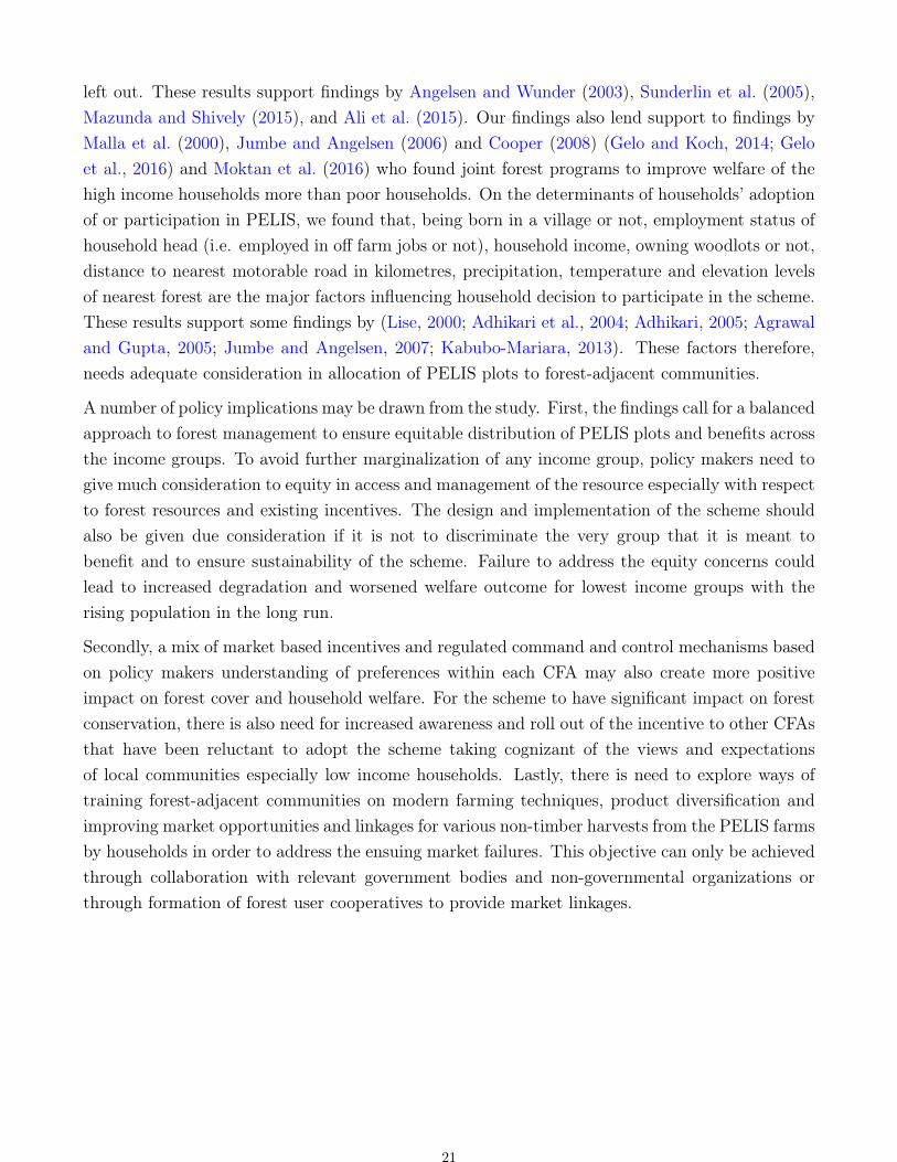
We considered a range of matches namely the nearest neighbor matching, radius matching, andkernel matching29. However, we selected the matches that resulted in highest number of balancedcovariates and large sample size within the common support as presented in Table 3. The kerneldensity showing the common support before and after matching is shown in Figure 1 in the annex.The figure shows a considerable magnitude of overlap after matching. Table 3 presents the qualityand performance of the matches selected out of the different matches used. The Columns of interestare labelled (1) & (2) and (6) & (7). Fourteen and thirteen explanatory variables were used at thehousehold level and CFA level analysis respectively30.

28We tried to tease out the determinants of households participation in PELIS at both CFA and household levels to assess therobustness of our household level determinants which was the main interest.

29It is important to note that, the choice of matching algorithm often involves a trade-off in terms of bias and efficiency.30A balance test of fourteen and thirteen variables in Column (1) and (6) suggests complete balance in matching. Whereas, the

pseudo R squared in Column (2) and (7) shows the explanatory power for the re-estimated propensity score model after matching.From literature, a number of criteria have been suggested to gauge the performance of matching estimators. The criteria include:checking if after matching the significant mean difference across covariates remains. An alternative involves re-estimating the probitregression using the matched sample (see Sianesi, 2004). There should be no systematic differences between the covariates after matchinghence the pseudo R squared should be low (Caliendo and Kopeinig, 2008). A likelihood ratio test of joint significance should also berejected before matching but not after.

16

Table 3: Performance of Matching estimator

Household Level CFA level(1) (2) (3) (4) (5) (6) (7) (8) (9) (10)

Matching estimator Bal test* Ps R2 LR chi2 P>ch2 Matched n Bal test* Ps R2 LR chi2 P>ch2 Matched nNN (4) 11 0.048 24.44 0.041 362 11 0.055 10.50 0.653 207NN (5) 11 0.047 24.08 0.045 362 12 0.047 9.07 0.768 207Radius (=0.0025) 14 0.033 9.89 0.770 284 13 0.073 6.26 0.936 169Radius (=0.005) 11 0.046 19.46 0.148 331 13 0.036 5.07 0.974 189* covariates with insignificant mean difference between beneficiaries and non-beneficiaries after matching

5.3.2 Matching Based treatment effects on PELIS beneficiaries

We present the estimated ATT in Table 4. The ATT were estimated for household welfare andCFA forest cover using psmatch2 command in stata (Leuven et al., 2015). The Columns of interestare labelled ATT and t-stat.

Table 4: Matching based Treatment Effects on PELIS beneficiaries

Per Capita Monthly Expenditure Forest coverEstimator ATT S.Dev t-stat ATT S.Dev t-statNN (4) 597.02 192.32 3.10*** 5.71 3.33 1.71*NN (5) 589.65 197.55 2.98*** 5.53 3.31 1.67*Radius (0.0025) 363.48 204.68 1.78* 7.73 4.10 1.88*Radius (0.005) 678.36 211.28 3.21*** 7.94 3.30 2.40*****<0.01, **<0.05, *<0.1

The results show that PELIS has significant (both economically and statistically) positive impacton household welfare and forest cover. The average impact of the scheme on PELIS beneficiaries’per capita monthly expenditure was estimated at between ksh. 363 (USD 3.63) and ksh. 678 (USD6.78). Based on the average per capita monthly expenditure for households benefiting from PELISwhich is Ksh. 2,409 (USD 24.09), this accounts for between 15.09% and 28.14%. The impact of thescheme on forest cover was estimated at between 5.53% and 7.94%. However, since we includedeven the covariates that remained significantly different even after matching (i.e., distance tomarket, precipitation and temperature) in the outcome analysis, to assess the robustness of thePSM estimates, we also run a matched regression with controls (We find impact on per capitaexpenditure to be between Ksh. 436 (USD 4.36) and Ksh. 525 (USD 5.25 whereas, on forest coverit was estimated between 4.67% and 7.27%)31. It is also important to note that, matching is based

31We find that the results for the matched regression and the PSM are not any different. These results are however not presented inthis paper since they were used to assess the robustness of our PSM estimates.

17

on the unconfoundedness assumption which is not testable. We therefore conducted a sensitivityanalysis of the matching estimates.

5.3.3 Sensitivity Analysis of the Matching Estimates

PSM is based on the assumption that the researcher should be able to observe all variables simulta-neously influencing decision to participate in PELIS and the outcome variable (unconfoundednessor the conditional independence assumption) otherwise, the matching estimators may not be ro-bust due to the hidden bias (Rosenbaum, 2002). Estimating the extent of selection bias is quitecomplex especially due to the fact that we used non experimental data. We therefore employedRosenbaum (2005) bounding approach to test for robustness of the matching estimates to unob-served variables. Following Rosenbaum (2005) bounding method we examined the sensitivity ofthe match based treatment effects estimates with respect to potential deviations from conditionalindependence. The sensitivity analysis results are presented in Table 1032.

Looking at our sensitivity analysis results in Table 10, for per capita expenditure, at Γ=1.2 and1.3 the results will not be significant at 1% and at Γ=1.4 the result is also not significant at 10%with p-value of 0.150. Whereas for forest cover, at Γ=1.1 the result will not be significant at10% with a p-value of 0.158. This suggests that unobserved covariates would cause the odds ratioof treatment assignment to differ between the participants and non-participants once we reach aspecific Γ level. From this results, we can infer that the results to some extent reveals some levelsof selectivity bias33.

Due to possibility of selection bias, to ascertain the robustness of our PSM estimates, we alsoemployed instrumental variables estimation technique following Lewbel’s heteroscedasticity-basedinstrumental variable technique (see Lewbel (2012)) to test and address the potential endogeneityof participation in PELIS on per capita household expenditure and forest cover34. Based on thisapproach, our results in Table 11 revealed that, PELIS has significant positive impact on householdpercapita monthly expenditure estimated at Ksh. 1270 (USD 12.70) hence raising welfare for theaverage household by about 58%. On the other hand, the estimated impact of PELIS on forestcover was approximately 4.23% holding other factors constant35. These findings therefore resonates

32The first column contains the log odds of differential assignment due to unobserved heterogeneity, the second to fifth columns,contains the upper and lower bound significance levels respectively for the key outcome variables namely per capita monthly expenditureand percentage forest cover. The second to fifth columns examines the match based treatment effect for each measure of unobservablepotential selection bias. The lower bounds are of no interests since they hold under the assumption that the true ATT is underestimatedbut our ATT estimates are positive (Becker and Caliendo, 2007).

33According to Becker and Caliendo (2007), the critical of say Γ= 1.4 for per capita expenditure and 1.1 for forest cover is not anindication that unobserved heterogeneity exists and that there is no effect of the treatment on the outcome variable. The unconfound-edness assumption therefore cannot be justified using this test hence we cannot state whether the CIA assumption holds or not. Theresult just indicates that if any unobserved variable caused the odds ratio of treatment assignment to differ between treatment andcomparison groups by sayΓ=1.4 for per capita expenditure, then the confidence interval for the treatment effect would include zero (seeBecker and Caliendo 2007).

34The main advantage of this approach is that, it provides options for generating instruments and allows the identification of structuralparameters in models with endogeneity or mis-measured regressors when we do not have external instruments. The approach is alsocapable of supplementing weak instruments. Identification is consequently achieved by having explanatory variables that are uncorrelatedwith the product of heteroscedastic errors (see Lewbel (2012)).

35In the two models, we first tested for endogeneity using the Durbin-Wu-Hausman tests for endogeneity and control function approachunder the null hypothesis that the variables are exogenous. The tests rejects the null hypothesis of exogeneity at 1% significance level for

18

well with the results from our PSM estimates although the impact on household welfare was foundto be slightly higher compared to the PSM estimates36.

5.4 Quantile Treatment Effects Model

To examine the impact of the scheme across the income distribution, the study adopted theendogenous QTE model. Since participation in PELIS is potentially endogenous to per capitaexpenditure, we first tested for endogeneity of participation in PELIS (our treatment variable).The control function approach was used to test for endogeneity. The approach is conducted intwo stages. In the first stage, the endogenous variable which in our case is PELIS was regressedon the instrumental variable BornVil (i.e a dummy variable whether the household head is bornin a given village or not) and other explanatory variables and the predicted residuals saved37. Inthe second step, the outcome variable (per capita expenditure) was regressed on the endogenousvariable, other explanatory variables and the residuals38 (Wooldridge, 2010). Using this test,the null hypothesis of exogeneity is rejected with a p-value of 0.05539. In light of evidence ofendogeneity of participation in PELIS, we proceeded to estimate an endogenous QTE model tohandle selection bias and solve the endogeneity problems. The results of the endogenous QTEmodel following Abadie et al. (2002) are presented in Table 12 in the appendix.

Conditioned on a set of covariates40, the endogenous QTE model revealed that the scheme hadsignificant positive impact on household welfare from the fourth to the ninth quantiles only showingthe distributional inequity of the scheme41. A major observation during the survey was the factthat, most forest-adjacent households participating in PELIS were mainly involved in growing thesame kind of crops i.e., peas, cabbages or potatoes which they complained that since they allharvested at almost the same time, this resulted in excess supply hence lower prices coupled withlack of market for the agricultural produce. Moreover, most forest-adjacent communities are poorhence have very limited alternatives in terms of exploring market opportunities for their produce,and even if the harvest is good, very few can afford to transport their produce to other areasthe two models. We also carried out performance statistics for the IV models. We tested for, under-identifcation based on Kleibergen-Paap rk Lm statistics, weak identification using the Donald Wald F statistics, and the Hansen J statistics under the null hypothesisthat the instruments are valid. The models passed all the tests hence proving that the heteroskedasticity-based IV estimates wouldyield reliable estimates.

36It is also important to note that we also arrive at similar conclusion when we used the endogenous switching regression model.37We computed the proportion of the predicted probabilities outside the unit interval. Finding only 6.4% fell outside the unit interval

we chose the LPM over the probit or logit model since the LPM would still produce unbiased and consistent estimates (Horrace andOaxaca, 2006). The F value for the LPM model was also found to be 11.15 with a p value of 0.000 showing the significance of the LPMmodel.

38The approach is same as the 2SLS approach but the only difference is that it allows for testing for endogeneity of PELIS participation.It however hinges on assumption of exogeneity of the instrument.

39The null hypothesis of exogeneity is also rejected when we use the Durbin-Wu-Hausman test of endogeneity at 1% significance level.40Namely, level of households participation in CFA activities, ownership of land titles, employment status, sex of household head and

whether the household head is a native or not, climate and geographical variables and distance to the nearest; market, main road, andthe nearest edge of the forest, among other factors.

41One anonymous reviewer suggested that we limit the quantiles to about five instead of the nine employed in the study. A reductionof the quantiles to five does not change the results because it simply estimates the impact at that quantiles but the results remainthe same. Since we were more interested in the entire income distribution leaving the quantiles at nine provided more information onthe true impact of the scheme at each and every segment. It is also important to note that, even if we employed the exogenous QTEmodel, we arrive at similar conclusion. The same was also the case when we used household percapita income as opposed to percapitaexpenditure.

19

to fetch better prices for their produce. Another possible reason could be due to elite captureissues where richer elite households take over the scheme and other CFA activities in general andtherefore set to benefit more than the poor households. This could therefore explain the inequitabledistributional nature of the scheme.

We therefore reject the null hypothesis of constant impact of the scheme on household welfarebecause the benefits are more skewed towards the middle and upper quantile households. How-ever, according to the Kenya Integrated Household Budget Survey (2005), the per capita monthlyexpenditure for rural households in the Rift valley province in which the Mau forest is located isapproximately Ksh 2251(USD 22.51). Comparing this with our average per capita monthly expen-diture for the sampled households which is about Ksh. 2185(USD 21.85), we find that the studypopulation is on average slightly below the poverty line. This shows that most households livingaround the Mau forest are relatively poor as has been shown by most studies that, the rural poorare the most forest dependent. However, the poverty datum line lies between the sixth (averageof Ksh 2082.26(USD20.82)) and 7th (average of ksh 2375.71(USD23.76)) quantiles see Table 9.Those below the poverty datum line are thus considered poor i.e. first to sixth quantile. It istherefore, evident that the scheme raised welfare of the poor but the least poor (fourth to sixthquantile households) and the richer quantile households benefit more from the scheme than thepoorest.

6 Conclusion and Policy Recommendations

The study aimed at identifying the determinants of household decision to participate in/adoptPELIS, and to determine the overall and distributional impact of PELIS on welfare of forest-adjacent households as well as the mean impact on forest cover. The PSM method estimated theimpact of PELIS on household per capita monthly expenditure at between ksh. 363 (USD 3.63)and ksh. 678 (USD 6.78) hence raising welfare by between 15.09% and 28.14% whereas the overallimpact of the scheme on forest cover was estimated at between 5.53% and 7.94% slightly lowerthan the OLS estimate of 9.45%. We can thus conclude that on average PELIS meets the dualobjective of raising household welfare and improving forest cover. This shows that devolution offorest management and provision of incentives to well organized communities can lead to betterwelfare and environmental outcomes on average. On the other hand, in terms of welfare, the QTEmodel under endogenous assumption, revealed that the scheme had positive impact on householdwelfare from the fourth quantile households and above only. We can therefore, infer that thereis some distributional inequity on the impact of the scheme that needs to be addressed for thesustainability and success of the scheme and for it to be able to make low income household riseup the income ladder and also lead to improvement in forest cover at the same time.

However, we cannot conclude that the scheme is less pro poor since the scheme raises welfare ofthe least poor as well even though the poorest and marginalized sections of the community are

20

left out. These results support findings by Angelsen and Wunder (2003), Sunderlin et al. (2005),Mazunda and Shively (2015), and Ali et al. (2015). Our findings also lend support to findings byMalla et al. (2000), Jumbe and Angelsen (2006) and Cooper (2008) (Gelo and Koch, 2014; Geloet al., 2016) and Moktan et al. (2016) who found joint forest programs to improve welfare of thehigh income households more than poor households. On the determinants of households’ adoptionof or participation in PELIS, we found that, being born in a village or not, employment status ofhousehold head (i.e. employed in off farm jobs or not), household income, owning woodlots or not,distance to nearest motorable road in kilometres, precipitation, temperature and elevation levelsof nearest forest are the major factors influencing household decision to participate in the scheme.These results support some findings by (Lise, 2000; Adhikari et al., 2004; Adhikari, 2005; Agrawaland Gupta, 2005; Jumbe and Angelsen, 2007; Kabubo-Mariara, 2013). These factors therefore,needs adequate consideration in allocation of PELIS plots to forest-adjacent communities.

A number of policy implications may be drawn from the study. First, the findings call for a balancedapproach to forest management to ensure equitable distribution of PELIS plots and benefits acrossthe income groups. To avoid further marginalization of any income group, policy makers need togive much consideration to equity in access and management of the resource especially with respectto forest resources and existing incentives. The design and implementation of the scheme shouldalso be given due consideration if it is not to discriminate the very group that it is meant tobenefit and to ensure sustainability of the scheme. Failure to address the equity concerns couldlead to increased degradation and worsened welfare outcome for lowest income groups with therising population in the long run.

Secondly, a mix of market based incentives and regulated command and control mechanisms basedon policy makers understanding of preferences within each CFA may also create more positiveimpact on forest cover and household welfare. For the scheme to have significant impact on forestconservation, there is also need for increased awareness and roll out of the incentive to other CFAsthat have been reluctant to adopt the scheme taking cognizant of the views and expectationsof local communities especially low income households. Lastly, there is need to explore ways oftraining forest-adjacent communities on modern farming techniques, product diversification andimproving market opportunities and linkages for various non-timber harvests from the PELIS farmsby households in order to address the ensuing market failures. This objective can only be achievedthrough collaboration with relevant government bodies and non-governmental organizations orthrough formation of forest user cooperatives to provide market linkages.

21

References

Abadie, A., Angrist, J., and Imbens, G. (2002). Instrumental variables estimates of the effect ofsubsidized training on the quantiles of trainee earnings. Econometrica, 70(1):91–117.

Adhikari, B. (2005). Poverty, property rights and collective action: Understanding the distributiveaspects of common property resource management. Environment and Development Economics,10(01):7–31.

Adhikari, B., Di Falco, S., and Lovett, J. C. (2004). Household characteristics and forest depen-dency: Evidence from common property forest management in Nepal. Ecological economics,48(2):245–257.

Agrawal, A. and Gupta, K. (2005). Decentralization and participation: The governance of commonpool resources in Nepals Terai. World development, 33(7):1101–1114.

Ali, A., Behera, B., et al. (2015). Household participation and effects of community forest man-agement on income and poverty levels: Empirical evidence from Bhutan. Forest Policy andEconomics, 61:20–29.

Angelsen, A. and Wunder, S. (2003). Exploring the forest–poverty link: Key concepts, issues andresearch implications. Technical report, CIFOR, Bogor, Indonesia.

Austin, P. C., Grootendorst, P., and Anderson, G. M. (2007). A comparison of the ability ofdifferent propensity score models to balance measured variables between treated and untreatedsubjects: A monte carlo study. Statistics in medicine, 26(4):734–753.

Becker, S. O. and Caliendo, M. (2007). mhbounds: Sensitivity Analysis for Average TreatmentEffects. Technical report, DIW Discussion Papers.

Blaikie, P. and Jeanrenaud, S. (1997). Biodiversity and human welfare. Social change and conser-vation. Earthscan, London, pages 46–70.

Caliendo, M. and Kopeinig, S. (2008). Some practical guidance for the implementation of propen-sity score matching. Journal of economic surveys, 22(1):31–72.

Chernozhukov, V. and Hansen, C. (2008). Instrumental variable quantile regression: A robustinference approach. Journal of Econometrics, 142(1):379–398.

Cooper, C. (2007). Distributional consideration of forest co-management in heterogeneous com-munity: Theory and simulation. Technical report, working paper, Department of Economics,University of Southern California.

22

Cooper, C. (2008). Welfare effects of community forest management: Evidences from hills of Nepal.Technical report, Working paper, Department of Economics, University of Southern California.

Fisher, M. (2004). Household welfare and forest dependence in Southern Malawi. Environmentand Development Economics, 9(02):135–154.

Force, P. M. T. (2009). Report of the Prime Ministers Task Force on the conservation of the MauForests Complex. Nairobi, Kenya.

Frölich, M. and Melly, B. (2010). Estimation of quantile treatment effects with stata. Stata Journal,10(3):423.

FSK (2006). Kenya forestry in the new millennium and the challenges facing a forester under theForestry Act No 7 of 2005. Forest Society of Kenya.

Gbadegesin, A. and Ayileka, O. (2000). Avoiding the mistakes of the past: towards a communityoriented management strategy for the proposed National Park in Abuja-Nigeria. Land UsePolicy, 17(2):89–100.

Gelo, D. and Koch, S. F. (2014). The impact of common property right forestry: Evidence fromEthiopian villages. World Development, 64:395–406.

Gelo, D., Muchapondwa, E., and Koch, S. F. (2016). Decentralization, market integration andefficiency-equity trade-offs: Evidence from Joint Forest Management in Ethiopian villages. Jour-nal of Forest Economics, 22:1–23.

Heckman, J. J., Ichimura, H., and Todd, P. (1998). Matching as an econometric evaluationestimator. The Review of Economic Studies, 65(2):261–294.

Heckman, J. J., LaLonde, R. J., and Smith, J. A. (1999). The economics and econometrics ofactive labor market programs. Handbook of labor economics, 3:1865–2097.

Horrace, W. C. and Oaxaca, R. L. (2006). Results on the bias and inconsistency of ordinary leastsquares for the linear probability model. Economics Letters, 90(3):321–327.

Jumbe, C. B. and Angelsen, A. (2007). Forest dependence and participation in cpr management:Empirical evidence from forest co-management in Malawi. Ecological Economics, 62(3):661–672.

Jumbe, C. B. L. and Angelsen, A. (2006). Do the poor benefit from devolution policies? Evidencefrom Malawi’s forest co-management program. Land Economics, 82(4):562–581.

Kabubo-Mariara, J. (2013). Forest-poverty nexus: Exploring the contribution of forests to rurallivelihoods in Kenya. In Natural Resources Forum, volume 37, pages 177–188. Wiley OnlineLibrary.

Kagombe, J. K. and Gitonga, J. (2005). Plantation establishment in kenya: The shamba systemcase study. Kenya Forestry Research Institute.

23

Khandker, S. R., Koolwal, G. B., and Samad, H. A. (2009). Handbook on impact evaluation:quantitative methods and practices. World Bank Publications.

Kumar, S. (2002). Does participation in common pool resource management help the poor? Asocial cost benefit analysis of joint forest management in Jharkhand, India. World Development,30(5):763–782.

Leuven, E., Sianesi, B., et al. (2015). Psmatch2: Stata module to perform full mahalanobisand propensity score matching, common support graphing, and covariate imbalance testing.Statistical Software Components.

Lewbel, A. (2012). Using heteroscedasticity to identify and estimate mismeasured and endogenousregressor models. Journal of Business & Economic Statistics.

Lise, W. (2000). Factors influencing people’s participation in forest management in india. Ecologicaleconomics, 34(3):379–392.

Malla, Y. B. et al. (2000). Impact of community forestry policy on rural livelihoods and foodsecurity in Nepal. Unasylva (English ed.), 51(202):37–45.

Maslow, A. H. (1943). A theory of human motivation. Psychological review, 50(4):370.

Maslow, A. H. (1991). Critique of self-actualization theory. The Journal of Humanistic Counseling,29(3):103–108.

Mazunda, J. and Shively, G. (2015). Measuring the forest and income impacts of forest user groupparticipation under Malawi’s Forest Co-management Program. Ecological Economics, 119:262–273.

MENR (2005). The Kenya Forests Act,. Ministry of Environment and Natural Resources.

MENR (2016). The Kenya Forest Act, 2016. Ministry of Environment and Natural Resources.

Moktan, M. R., Norbu, L., and Choden, K. (2016). Can community forestry contribute to house-hold income and sustainable forestry practices in rural area? A case study from Tshapey andZariphensum in Bhutan. Forest Policy and Economics, 62:149–157.

NEMA (2013). Mau Complex at a Glance. Nairobi, Kenya.

Rosenbaum, P. R. (2002). Observational studies. In Observational studies, pages 1–17. Springer.

Rosenbaum, P. R. (2005). Sensitivity analysis in observational studies., volume 4.

Roy, A. D. (1951). Some thoughts on the distribution of earnings. Oxford economic papers,3(2):135–146.

Rubin, D. B. (1973). Matching to remove bias in observational studies. Biometrics, pages 159–183.

24

Rubin, D. B. (1974). Estimating causal effects of treatments in randomized and nonrandomizedstudies. Journal of educational Psychology, 66(5):688.

Rubin, D. B. (1979). Using multivariate matched sampling and regression adjustment to controlbias in observational studies. Journal of the American Statistical Association, 74(366a):318–328.

Sianesi, B. (2004). An evaluation of the swedish system of active labor market programs in the1990s. Review of Economics and statistics, 86(1):133–155.

Skoufias, E. and Katayama, R. S. (2011). Sources of welfare disparities between and within regionsof brazil: Evidence from the 2002–2003 household budget survey (pof). Journal of EconomicGeography, 11(5):897–918.

Sterner, T. (2003). Policy instruments for environmental and natural resource management. Re-sources for the Future.

Stock, J. H. and Yogo, M. (2005). Testing for weak instruments in linear IV regression. Identifi-cation and inference for econometric models: Essays in honor of Thomas Rothenberg.

Sunderlin, W. D., Angelsen, A., Belcher, B., Burgers, P., Nasi, R., Santoso, L., and Wunder,S. (2005). Livelihoods, forests, and conservation in developing countries: An overview. Worlddevelopment, 33(9):1383–1402.

UNEP (2008). CDM/JI Pipeline Analysis and Database, March 1st 2008. RISCOE, RoskildeDenmark.

Wooldridge, J. M. (2010). Econometric analysis of cross section and panel data. MIT Press.

WorldBank (2000). Third forestry project. Unpublished report.

Wunder, S. (2001). Poverty alleviation and tropical forests what scope for synergies? Worlddevelopment, 29(11):1817–1833.

25

Appendix

Table 5: Description of VariablesVariable DefinitionDependent variablesPCMonthlyExp Per capita Monthly ExpenditureForestcover Forest Cover expressed as a percentage of total forest size under each CFAExplanatoryHHWealth Total value of household asserts (land, farm animals, agricultural implements, farm produce etc)PELIS Dummy=1 if household owns a PELIS plot and 0 otherwiseHHsex Dummy=1 if Male and 0 if femaleNumbchild Number of childrenBornVil Dummy=1 if born in the village, 0 otherwiseMedAge Age of the household head (Median age calculated from the categorical variables)hhsize Number of people in the household including household headMaritSta Dummy=1 if married, 0 not marriedEducation Dummy=1 if household head has post primary education and

0 if household head has up to primary educationResidStatus Dummy=1 if household head is a native, 0 if household head is an immigrant/settlerHHEducyrs Years of educationMultilingual Dummy=1 if speaks more than two languages, 0 if speak two or less languagesEmployment Status Dummy=1 if employed in off farm, 0 if self employed i.e farmingLandTitle Dummy=1 if Own title for household land, 0 otherwiseMedIncome Median monthly income for the householdWoodlots Dummy=1 If the household owns a woodlot, 0 otherwiseCFAMeeting Dummy=1 If father represents the household in CFA meetings,

0 if Mother represents the HouseholdCFAParticipation Dummy=1 If the household is active in participation in CFA activities, 0 if passiveHsepartic Dummy=1 if household participates in CFA activities, 0 otherwiseHlandsize Size of household landHownership Dummy=1 if the household head owns the house, 0 otherwiseDistMroad Distance from household to the nearest motorable road in kmDistMarket Distance from household to the nearest market using in kmDistForest Distance from household to the nearest edge of the forest in kmMembership Dummy=1 if a member of other environmental organizations(e.g. CBOs), 0 otherwiseTemperature Annual average temperature in degrees CelsiusPrecipitation Average Annual precipitation (mm)Elevation Level of Elevation in each forest (meters)

26

Table 6: Summary StatisticsTotal Sample PELIS Beneficiaries Non PELIS Beneficiaries

variable N Mean sd N Mean sd N Mean sdDependentPCMonthlyExp 406 2186 1615 228 2405 1939 178 1905 1003Forestcover 267 77.64 14.23 137 79.54 10.47 130 75.64 17.15ExplanatoryHHWealth 406 1.269e+06 1.759e+06 228 1.257e+06 2.043e+06 178 1.284e+06 1.311e+06HHsex 405 0.780 0.415 227 0.767 0.424 178 0.798 0.403Numbchild 406 4.865 2.701 228 5.171 2.729 178 4.472 2.619BornVil 405 0.585 0.493 228 0.531 0.500 177 0.655 0.477MedAge 406 48.14 13.73 228 49.29 12.70 178 46.67 14.85hhsize 406 5.798 2.631 228 6.110 2.729 178 5.399 2.450MaritSta 406 0.869 0.337 228 0.895 0.308 178 0.837 0.370Education 406 0.360 0.480 228 0.351 0.478 178 0.371 0.484ResidStatus 406 0.574 0.495 228 0.570 0.496 178 0.579 0.495Hsepartic 406 0.904 0.295 228 0.908 0.290 178 0.899 0.302Employment 406 0.241 0.428 228 0.167 0.373 178 0.337 0.474LandTitle 406 0.522 0.500 228 0.513 0.501 178 0.534 0.500MedIncome 406 15788 20503 228 17862 25993 178 13132 9097HHEducyrs 406 8.404 3.639 228 8.329 3.556 178 8.500 3.751Woodlots 406 0.850 0.358 228 0.912 0.284 178 0.770 0.422CFAParticipation 406 0.623 0.485 228 0.697 0.460 178 0.528 0.501Hownership 406 0.904 0.295 228 0.917 0.277 178 0.888 0.317DistMroad 406 1.926 2.696 228 2.485 2.983 178 1.211 2.073DistMarket 406 3.368 3.537 228 3.885 3.504 178 2.707 3.478DistForest 406 1.481 1.478 228 1.406 1.408 178 1.578 1.561Hlandsize 406 2.519 5.682 228 2.473 7.020 178 2.578 3.263Membership 406 0.0690 0.254 228 0.0702 0.256 178 0.0674 0.251Temperature 406 15.05 1.776 228 15.51 1.726 178 14.46 1.667Precipitation 406 1164 181.4 228 1197 183.2 178 1122 170.7Elevation1 406 2444 233.4 228 2402 254.8 178 2499 189.9

27

Table 7: Descriptive Statistics

variable PELIS Beneficiaries Non PELIS Beneficiaries Mean Differencemean s.e mean s.e Mean s.e

PCMonthlyExp 2404.52*** (128.42) 1905.33*** (75.14) 499.19** (159.82)Forestcover 79.72*** (0.95) 75.73*** (1.41) 3.99*** (1.72)HHWealth 1.256e+06 (135333) 1.283e+06 (98298) 27294.18 (176098)HHsex 0.767*** (0.028) 0.798*** (0.030) -0.031 (0.042)Numbchild 5.171*** (0.181) 4.472*** (0.196) 0.699** (0.268)BornVil 0.531*** (0.033) 0.655*** (0.036) -0.125** (0.049)MedAge 49.285*** (0.841) 46.67*** (1.112) 2.611* (1.369)hhsize 6.109*** (0.181) 5.399*** (0.184) 0.711*** (0.261)MaritSta 0.895*** (0.020) 0.837*** (0.028) 0.058* (0.034)Education 0.351*** (0.032) 0.371*** (0.036) -0.019 (0.048)ResidStatus 0.570*** (0.033) 0.578*** (0.037) 0.008 (0.050)Hsepartic 0.907*** (0.019) 0.899*** (0.023) 0.009 (0.030)Multilingual 0.491*** (0.033) 0.438*** (0.037) 0.053 (0.050)Employment Status 0.167*** (0.025) 0.337*** (0.035) -0.170*** (0.042)LandTitle 0.513*** (0.033) 0.533*** (0.037) -0.021 (0.050)MedIncome 17862*** (1721.409) 13132*** (681.868) 4729.798** (2039.709)HHEducyrs 8.328*** (0.235) 8.500*** (0.281) -0.171 (0.364)Woodlots 0.912*** (0.019) 0.770*** (0.032) 0.143*** (0.035)CFAParticipation 0.697*** (0.030) 0.528*** (0.038) 0.169*** (0.048)Hownership 0.917*** (0.018) 0.888*** (0.024) 0.029 (0.030)DistMroad 2.485*** (0.198) 1.211*** (0.155) 1.274*** (0.262)DistMarket 3.885*** (0.232) 2.707*** (0.261) 1.177*** (0.349)DistForest 1.406*** (0.093) 1.578*** (0.117) -0.173 (0.148)Hlandsize 2.473*** (0.465) 2.578*** (0.245) -0.104 (0.569)Membership 0.0702*** (0.017) 0.0674*** (0.019) 0.003 (0.025)Temperature 15.51*** (0.114) 14.46*** (0.125) 1.044*** (0.170)Precipitation 1197*** (12.134) 1122*** (12.792) 74.437*** (17.787)Elevation 2401*** (16.875) 2498*** (14.233) -97.059*** (22.869)Table of mean differences and test of significance. Standard errors in parentheses *** p<0.01, ** p<0.05, * p<0.1

Table 8: Per Capita Monthly Expenditure across the quantilesQuantile Mean PCMonthly Exp No of Households

1st Quantile 695.19 462nd Quantile 1111.58 473rd Quantile 1370.93 434th Quantile 1596.29 455th Quantile 1847.10 456th Quantile 2082.26 457th Quantile 2375.71 458th Quantile 3019.14 469th Quantile 5673.27 44

All households 2185 406

28

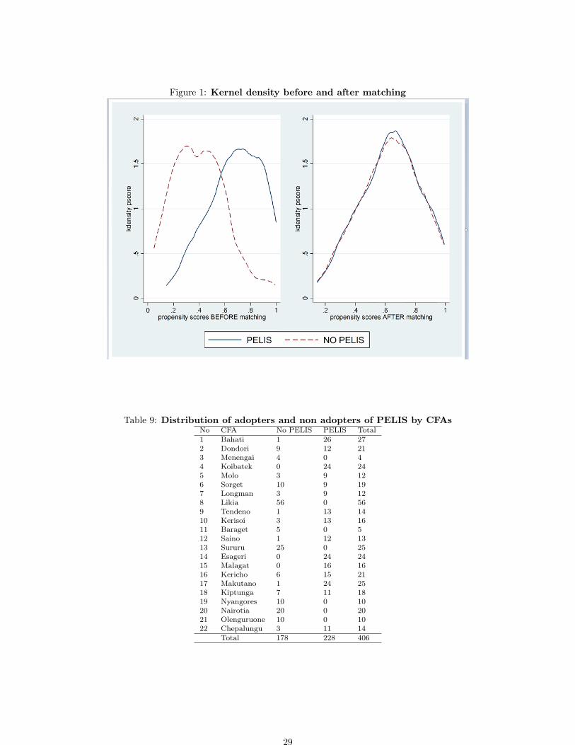
Figure 1: Kernel density before and after matching

Table 9: Distribution of adopters and non adopters of PELIS by CFAsNo CFA No PELIS PELIS Total1 Bahati 1 26 272 Dondori 9 12 213 Menengai 4 0 44 Koibatek 0 24 245 Molo 3 9 126 Sorget 10 9 197 Longman 3 9 128 Likia 56 0 569 Tendeno 1 13 1410 Kerisoi 3 13 1611 Baraget 5 0 512 Saino 1 12 1313 Sururu 25 0 2514 Esageri 0 24 2415 Malagat 0 16 1616 Kericho 6 15 2117 Makutano 1 24 2518 Kiptunga 7 11 1819 Nyangores 10 0 1020 Nairotia 20 0 2021 Olenguruone 10 0 1022 Chepalungu 3 11 14

Total 178 228 406

29

Table 10: Sensitivity Analysis of Matching EstimatesPCMonthlyExp Forest Cover

Gamma sig+ sig- sig+ sig-1 0.00141 0.00141 0.0956 0.0956

1.100 0.00759 0.000191 0.167 0.04931.200 0.0273 2.30e-05 0.256 0.02441.300 0.0720 2.50e-06 0.356 0.01171.400 0.150 2.50e-07 0.457 0.005491.500 0.261 2.40e-08 0.554 0.002521.600 0.393 2.20e-09 0.643 0.001141.700 0.529 1.90e-10 0.719 0.0005061.800 0.655 0 0.784 0.0002231.900 0.761 0 0.836 9.70e-052 0.842 0 0.877 4.20e-05

*gamma: Log odds of differential assignment due to unobserved factorssig+ : Upper bound significance level, sig-: Lower bound significance level

30

Table 11: Heteroscedasticity Based Instrumental Variable Estimation Results

(1) (2)VARIABLES PCMonthlyExp ForestcoverPELIS 1,270** 4.229**

(635.6) (2.051)HHsex -184.0 0.439

(191.7) (1.366)EmploymentStat -236.4 -0.261

(185.9) (1.427)LandTitle 285.3** 0.767

(139.8) (1.135)Woodlots -162.4 0.225

(247.1) (1.644)ResidStatus -260.1 -0.0392

(233.8) (2.297)CFAParticipation 151.9 2.244*

(155.6) (1.253)Hsepartic -522.2* 4.153***

(302.2) (1.504)DistForest -98.40** -0.981***

(44.75) (0.349)DistMroad 43.32 -0.126

(42.18) (0.305)DistMarket 13.10 0.699***

(25.45) (0.238)HHEducyrs 85.65*** -0.0167

(23.36) (0.165)Hlandsize 4.909 -0.208**

(19.86) (0.0953)hhsize -292.4*** 0.0641

(36.34) (0.269)HHWealth 0.000127 6.00e-07

(9.53e-05) (4.43e-07)Numbchild 41.08 0.246

(38.94) (0.295)MedAge 4.254 -0.481**

(41.05) (0.239)MedAgesq -0.0577 0.00374*

(0.351) (0.00207)MedIncome 0.0126* 1.64e-05

(0.00745) (1.95e-05)Temperature -191.3*** -3.827***

(58.40) (0.463)BornVil 58.28 -5.203**

(263.5) (2.286)Precipitation 0.0920 -0.0748***

(0.427) (0.00665)Membership 175.3 0.637

(315.4) (1.683)Other ControlsInstitutional variables No YesConstant 5,279*** 212.7***

(1,322) (13.60)Observations 404 404R-squared 0.351 0.721Robust standard errors in parentheses *** p<0.01, ** p<0.05, * p<0.1

31

Table 12: Endogenous Quantile Treatment Effects Model Estimation Results

VARIABLES QT_1 QT_2 QT_3 QT_4 QT_5 QT_6 QT_7 QT_8 QT_9PELIS -75.21 167.2 410.6 497.6* 532.8** 565.7** 842.7*** 1,227*** 2,155***

(194.2) (382.0) (328.1) (288.5) (246.8) (258.9) (269.8) (411.2) (787.1)DistForest -105.3** 0.379 -68.29 -78.10* -44.18 -48.76 -176.6*** -278.4*** -256.2***

(44.52) (53.86) (51.67) (43.28) (36.85) (52.45) (41.57) (54.36) (81.45)DistMroad 44.76 -37.09 -46.65 39.06 71.89** 60.14 -30.60 -74.81 -109.9

(40.70) (33.26) (43.54) (41.68) (31.16) (49.19) (41.81) (55.22) (201.7)DistMarket -96.78*** -32.88 -24.18 -60.19*** -44.54*** -44.82*** -24.29 -28.87 -13.12

(17.33) (20.12) (19.77) (12.21) (12.27) (15.03) (20.85) (24.27) (34.17)HHEducyrs -18.78 -7.228 -24.11** -17.48* -11.81 -7.174 -3.824 1.239 -11.10

(12.23) (12.31) (10.18) (9.067) (7.749) (10.88) (9.992) (12.23) (24.31)Hlandsize 40.53 54.70*** 44.86* -2.354 -22.62* -38.10*** -50.85*** -59.33*** -65.26

(32.85) (19.62) (24.00) (17.38) (12.21) (13.01) (14.53) (15.60) (43.60)hhsize -234.7*** -182.9*** -146.0*** -177.7*** -190.8*** -188.7*** -205.6*** -238.5*** -176.3***

(22.71) (41.35) (40.11) (26.38) (25.00) (34.31) (29.02) (42.79) (67.18)HHWealth 0.000139 0.000206 0.000296* 0.000523*** 0.000549*** 0.000566*** 0.000562*** 0.000698*** 0.000560***

(0.000247) (0.000142) (0.000169) (8.65e-05) (6.84e-05) (6.59e-05) (7.17e-05) (7.39e-05) (0.000160)Numbchild -20.56 -8.951 -56.16*** -37.01*** -21.85 -7.822 39.44 -31.97 -7.319

(24.37) (16.36) (13.27) (14.22) (15.07) (30.68) (37.93) (41.56) (110.5)MedAge 45.19*** 29.17 1.164 -27.36 -64.09*** -55.01* -58.92* 7.636 -58.54

(17.36) (27.95) (35.95) (28.08) (20.01) (28.24) (32.84) (52.46) (77.39)MedAgesq -0.305* -0.186 0.0919 0.466 0.742*** 0.650** 0.469 -0.0834 0.517

(0.181) (0.305) (0.364) (0.288) (0.201) (0.292) (0.335) (0.556) (0.813)MedIncome 0.0156*** 0.0151*** 0.0134*** 0.0111*** 0.0110*** 0.0200 0.0225*** 0.0257** 0.0416

(0.00462) (0.00358) (0.00447) (0.00350) (0.00425) (0.0198) (0.00606) (0.0112) (0.0465)Temperature 72.20*** 58.22*** -2.278 -8.517 -24.80 25.56 34.19 35.31 43.11

(24.37) (13.73) (17.73) (15.73) (16.62) (55.72) (38.63) (35.60) (115.6)Precipitation -1.084*** -1.142*** -1.217*** -1.270*** -1.248*** -1.773*** -1.780*** -2.663*** -2.560***

(0.241) (0.167) (0.133) (0.139) (0.139) (0.289) (0.240) (0.381) (0.714)HHsex 578.2** 443.8*** 331.5* 494.8*** 325.2 -81.67 -327.6 -694.6* -1,029*

(274.7) (170.5) (191.5) (160.9) (201.7) (265.1) (310.8) (388.3) (530.3)EmploymentStat -178.5*** 203.6** 58.19 171.7* 86.88 -147.0 -395.8*** -364.4** -385.8**

(64.71) (85.42) (92.32) (88.03) (88.08) (188.7) (117.0) (171.6) (156.5)LandTitle -291.0 -378.4*** -285.1** -315.1*** -279.8*** -187.5* 159.5 608.8*** 893.4***

(190.1) (137.0) (115.3) (68.39) (58.40) (103.6) (111.2) (172.6) (270.0)Woodlots 132.2 8.014 65.88 164.9*** 136.1** 16.68 114.8 138.3 372.9

(199.8) (110.4) (102.2) (54.66) (63.22) (124.2) (108.0) (144.3) (544.7)Membership 94.31 10.91 -100.3 -273.2 -156.5 -59.05 -356.1* -325.6 -233.0

(132.4) (150.5) (183.4) (177.6) (156.1) (189.1) (204.3) (220.6) (280.5)ResidStatus -195.7** -223.7** 35.68 154.4* 140.0* -4.487 -34.03 -358.2*** -396.1

(97.44) (103.8) (112.4) (84.54) (81.65) (143.8) (140.9) (104.5) (320.6)CFAParticipation 224.0** 312.6*** 375.5*** 606.7*** 453.3*** 593.6*** 364.5*** 392.9*** 507.4***

(92.38) (68.11) (81.77) (79.54) (90.47) (190.3) (137.6) (147.4) (145.5)Hsepartic 435.2*** 345.6*** 433.1*** 409.6*** 477.1*** 398.9* 257.1* 411.1** 278.4

(86.66) (55.30) (76.57) (69.12) (66.35) (239.9) (135.3) (185.7) (554.3)Constant 325.3 678.1 2,553*** 2,783*** 4,269*** 4,456*** 5,686*** 5,777*** 7,085***

(457.2) (604.1) (790.3) (497.4) (410.5) (640.2) (809.7) (1,308) (1,609)Observations 404 404 404 404 404 404 404 404 404

Standard errors in parentheses *** p<0.01, ** p<0.05, * p<0.1

32