Welcome!

Virtual tutorial starts at 15:00 GMT

Please leave feedback afterwards at: www.archer.ac.uk/training/feedback/online-course-feedback.php

Multi-resolution modelling of biological systems in

LAMMPS ARCHER Virtual Tutorial, 19th Oct 2016 Iain Bethune ibethune@epcc.ed.ac.uk

Oliver Henrich ohenrich@epcc.ed.ac.uk

Reusing this material

This work is licensed under a Creative Commons Attribution-NonCommercial-ShareAlike 4.0 International License.

http://creativecommons.org/licenses/by-nc-sa/4.0/deed.en_US

This means you are free to copy and redistribute the material and adapt and build on the material under the following terms: You must give appropriate credit, provide a link to the license and indicate if changes were made. If you adapt or build on the material you must

distribute your work under the same license as the original.

Note that this presentation contains images owned by others. Please seek their permission before reusing these images.

Outline • ARCHER eCSE programme

•  Implementation of Dual Resolution Simulation Methodology in LAMMPS •  ELBA force-field •  Implementation in LAMMPS •  Performance testing •  Summary

ARCHER eCSE programme •  Funding for the ARCHER user community to develop

software •  Implementation of algorithmic improvements within an existing code •  Improving the scalability of software on higher core counts •  Improvements to code which allows new science to be carried out •  Porting and optimising a code to run efficiently on ARCHER •  Adding new functionalities to existing codes •  Code development to take a code from a Tier-2 (Regional) or local

university cluster to Tier-1 (National) level bringing New Communities onto ARCHER

• Projects typically 3 months – 1 year • Next call closes 31st Jan 2017

ARCHER eCSE programme • More information on the ARCHER website:

•  https://www.archer.ac.uk/community/eCSE/ •  Project Reports •  How To Apply •  List of funded projects

• Webinar from last month: •  https://youtu.be/WRGsNKWrNIc

Implementation of Dual Resolution Simulation Methodology in LAMMPS

•  eCSE04-7 (January 2015) • PI: Prof. Jonathan Essex, Southampton •  6 person-months funded: August 2015 – August 2016

• Objective: enable fast and reliable calculations with the ELBA force-field in LAMMPS •  New integrators •  Parallel load balancing

ELBA Force-field • ELBA = ELectrostatics-BAsed coarse grained forcefield

•  Orsi & Essex, PLoS ONE 6(12) 2011

• Originally for studying lipids •  Also applied to other biomolecules

• Explicit solvent •  One dipolar bead per water molecule

• Allows for atomistic detail e.g. •  Using CHARMM parameters 138 atoms -> 15 CG beads

ELBA Force-field •  Implemented in BRAHMS-MD (Biomembrane Reduced-

ApproacH Multiresolution Simulator for Molecular Dynamics): •  https://code.google.com/archive/p/brahms-md/ •  Limited user base, single developer -> not sustainable •  No parallelisation -> small systems

• Why LAMMPS? •  Main interaction types already implemented •  Support for spherical particles •  r-RESPA multiple timestepping •  Flexible, scalable, large user base

http://lammps.sandia.gov

Implementation in LAMMPS •  LAMMPS fix nve/sphere integrator does not conserve energy well •  Better scheme to integrate rotational d.o.f. - DLM

Dullweber, Leimkuhler and McLachlan, JCP 107(15) 1997 1.  Construct rotation matrix Q from dipole (taken as the body-fixed z-axis) 2.  In body-space, apply rotations around each local axis:

3.  Finally, compute the new dipole:

Implementation of Dual Resolution SimulationMethodology in LAMMPS 5

Then the rotation matrix Q is given by:

Q = I + [v]⇥ + [v]2⇥

1 � cs2

Care has to be taken for the case were the dipole is parallel (or anti-parallel) to the

space-frame z-axis, in which case Q = I (or �I, respectively). In the DLM algorithm

the orientation is integrated by a sequence of rotations around each axis in the body-

frame, while LAMMPS stores the angular velocity in the space-frame. Thus compared to

the steps given in the DLM paper, our implementation has an additional transformation

step to compute the angular velocity in the body-frame, and due to the definition of the

orientation matrix, the orientation updates take the form of a right-multiplication by the

transpose of the rotation matrix. The rotation matrices for a rotation around each axis are

defined as (x rotation shown, the other two axes similarly):

Rx(�) =

266666666666666666666666664

1 0 0

0 cos � � sin �

0 sin � cos �

377777777777777777777777775

and implemented (in the MathExtra namespace), using the more e�cient small angle

approximations:

sin � =�

1 + �2/4, cos � =

1 � �2/41 + �2/4

The full rotational update is implemented as follows:

!b = Q!s

R1 = Rx(�t2!1), ! = R1!, Q = RT

1 Q

R2 = Ry(�t2!2), ! = R2!, Q = RT

2 Q

R3 = Rz(�t!3), ! = R3!, Q = RT3 Q

6 Implementation of Dual Resolution SimulationMethodology in LAMMPS

R4 = Ry(�t2!2), ! = R4!, Q = RT

4 Q

R5 = Rx(�t2!1), ! = R5!, Q = RT

5 Q

Finally, the space-frame dipole is computed as:

µs = QT [001] · ||µ||

To correctness of the implementation was tested on two systems. Firstly, a 49.34 Å3

cubic box containing 4000 ELBA water beads was equilibriated at 300K using a Langevin

thermostat for 10 ps, then the thermostat was removed and 10ps of MD in the microcanon-

ical (NVE) ensemble was performed. The timestep for both the entire run was 10fs using

fix nve/sphere update dipole. Two runs, one with the native ‘LAMMPS’ integra-

tor and one with our new ‘DLM’ integrator are shown in Figure 2. While the thermostat

is enabled equipartition of the kinetic energy is maintained in both cases. Once the ther-

mostat is removed, the ‘leaking’ of energy from the rotational modes is clear, and good

energy conservation is only obtained by using the DLM integrator.

Figure 2: Rotational and translational components of kinetic energy for a box of 4000ELBA water beads during 2000 steps of NVT and 2000 steps of NVE molecular dynam-ics.

A similar experiment was carried out with a simulation of a lipid membrane consisting

6 Implementation of Dual Resolution SimulationMethodology in LAMMPS

R4 = Ry(�t2!2), ! = R4!, Q = RT

4 Q

R5 = Rx(�t2!1), ! = R5!, Q = RT

5 Q

Finally, the space-frame dipole is computed as:

µs = QT [001] · ||µ||

To correctness of the implementation was tested on two systems. Firstly, a 49.34 Å3

cubic box containing 4000 ELBA water beads was equilibriated at 300K using a Langevin

thermostat for 10 ps, then the thermostat was removed and 10ps of MD in the microcanon-

ical (NVE) ensemble was performed. The timestep for both the entire run was 10fs using

fix nve/sphere update dipole. Two runs, one with the native ‘LAMMPS’ integra-

tor and one with our new ‘DLM’ integrator are shown in Figure 2. While the thermostat

is enabled equipartition of the kinetic energy is maintained in both cases. Once the ther-

mostat is removed, the ‘leaking’ of energy from the rotational modes is clear, and good

energy conservation is only obtained by using the DLM integrator.

Figure 2: Rotational and translational components of kinetic energy for a box of 4000ELBA water beads during 2000 steps of NVT and 2000 steps of NVE molecular dynam-ics.

A similar experiment was carried out with a simulation of a lipid membrane consisting

Implementation in LAMMPS •  4000 ELBA water beads, 10fs timestep, 20ps NVT, 20ps NVE fix thermostat all langevin 303 303 200 48279 omega yes

Implementation in LAMMPS •  128 DPMC molecules in water, 75ps NVT, 100ps NVE

Image from Sam Genheden

Implementation in LAMMPS •  DLM integrator enabled by an optional argument:

•  fix nve/sphere … update dipole/dlm

•  Also for other ensembles: •  Constant temperature / NVT (Nosé-Hoover) •  fix nvt/sphere … update dipole/dlm

•  Isothermal-isobaric (Nosé-Hoover / Parrinello-Rahman) •  fix npt/sphere … update dipole/dlm

•  Isenthalpic (Parrinello-Rahman) •  fix nph/sphere … update dipole/dlm

Implementation in LAMMPS •  Load balancing schemes:

None Shift RCB •  Problem for dual-resolution simulations!

•  90% of computational cost is force evaluation •  Not all particles are the same •  r-RESPA – some forces are computed more frequently than others

http://lammps.sandia.gov/doc/balance.html

Implementation in LAMMPS •  New load balancing metrics:

•  Weighting by particle groups •  Uses LAMMPS existing group command e.g. group solute type > 1

group water type 1

balance 1.1 shift xyz 50 1.1 weight group 1 solute 2.5

Threshold to start load balancing

Load balancing algorithm

Balance all 3 dimensions

Iteration limit

Threshold to stop balancing

Weight particles by group (1 group)

Solute group has weight factor 2.5

Implementation in LAMMPS •  New load balancing metrics (subsequently added by LAMMPS

developers):

•  Weighting by number of neighbors – weight neigh

•  Weighting by compute time – weight time •  Doesn’t account for the different particles types contributing to different parts of the

computation (pair, bond, kspace, neigh)

•  Weighting by arbitrary user-defined variables – weight var

Performance testing •  Bovine Pancreatic Trypsin Inhibitor (BPTI) dual-resolution model:

•  882 atoms, CHARMM force-field •  6136 water molecules, ELBA beads

•  No r-RESPA •  1fs timestep •  Up to 10%

speedup over non-weighted balance

Performance testing

•  1:4 r-RESPA ratio •  Water pair forces

+ dihedral forces computed every fourth step

•  Larger weightings better (2.5-3.0)

•  Up to 36% speedup over non-weighted balance

Performance testing

•  1:8 r-RESPA ratio •  Larger weightings

better (3.0-4.0) •  Up to 65%

speedup over non-weighted balance

Summary

•  DLM integrator for NVE/NVT/NPT/NPH dynamics •  Stable for water up to 16fs timestep •  Included in LAMMPS stable release 30 Jul 2016

•  New load balancing metrics •  Better performance for r-REPSA and hybrid pair force •  Include in LAMMPS patch release 27 Sep 2016

•  More information •  Technical Report:

http://www.archer.ac.uk/documentation/white-papers/lammps-elba/lammps-ecse.pdf •  Tutorials, references, discussion: https://sgenheden.github.io/Elba/

Installed on ARCHER module load

lammps/elba

ARCHER eCSE05-10 Project •  Adding Multiscale Models of DNA to LAMMPS (09/2015 – 08/2016) •  Dr Oliver Henrich (PI, UoE), Prof Davide Marenduzzo (Co-I, UoE),

Dr Thomas Ouldridge (Co-I, Imperial College London) •  Overview:

o  Implemented oxDNA coarse-grained DNA model for single- and double- stranded DNA into LAMMPS code

o  Implemented new Langevin-type rigid-body integrators o  Software available

from CCPForge (https://ccpforge.cse.rl.ac.uk/gf/project/cgdna) soon as LAMMPS USER-package

o  Currently adapting utility software of oxDNA standalone version

From DNA to Chromosomes •  Haploid human genome contains 3.2 billion

base pairs organised in 23 chromosomes o  Diameter of DNA strand = 2 x 10-9m o  Total length of DNA in human cell = 2m o  Diameter of spherical ‘blob’ of DNA in

human cell = 2 x 10-6m

•  Hierarchical organisation o  Histone octamer o  Nucleosome core particles 200 bps o  10 nm beads-on-a-string o  30 nm chromatin fibre o  smallest loop in chromatin fibre 50,000 bps

A−DNA B−DNA Z−DNA

Base Pairs Sugar−Phosphate Backbone

b)

a)Atomistic Simulation of DNA

•  Good for capturing fast conformational fluctuations and protein-DNA binding

•  Usually limited to a few 1000 base pairs

•  Phenomena on large time and length scales, e.g. DNA supercoiling or nucleosome positioning are permanently out of reach

Coarse-grained simulation with oxDNA

basebackbone

1 nucleotide

•  Must deliver correct longitudinal and torsional persistence length, electrostatics, if sequence-specific correct melting temperature, elastic constants …

•  oxDNA: top-down approach of a CG model, nucleotides modelled as rigid bodies (DOF are COM & quaternion)

•  Parameterize interaction between nucleotides with 6 independent interactions (7 for implicit electrostatics)

oxDNA Force Field

basebackbone

1 nucleotide

•  Backbone: FENE (finite extensible nonlinear elastic) springs •  Excluded volume: Lennard-Jones potential •  Stacking: harmonic angle x Morse potential •  Cross-stacking: harmonic angle x harmonic distance potential •  Coaxial stacking: harmonic angle x harmonic distance potential •  Hydrogen bonding: harmonic angle x Morse potential

oxDNA Force Field •  Smoothed, truncated and modulated forms of the above •  1 bonded interaction (backbone), 5 pair interactions (excluded volume,

stacking, hydrogen boding, cross-stacking, coaxial stacking)

δ

rstack

rHB

rback−baserbase

rbackbone

θ1

θ2

θ3

θ4

θ5

θ6

θ7

θ8

rbase−back

Backbone−base vectorBase normal

0.80 units0.74 units

δ

δ

δ

δδ

For full details see Thomas Ouldridge, Coarse-grained modelling of DNA and DNA self-assembly, DPhil, University of Oxford, 2011.

Parallel Performance

100

101

102

103

10 100 1000 10000

Spee

dup

vs 2

4 M

PI-ta

sks

MPI-tasks

LAMMPS- oxDNA Scaling

Ideal performance60 kbp

960 kbp

0

1

100 1000

Para

llel E

ffici

ency

MPI-tasks

Strong scaling for 60kbp and 960 kbp up to 8192 MPI-tasks

Benchmarks: •  Low density: array of 100 DNA

duplexes with 600 base pairs long (see above) = 60 kbp

•  High density: array of 1600 duplexes = 960 kbp

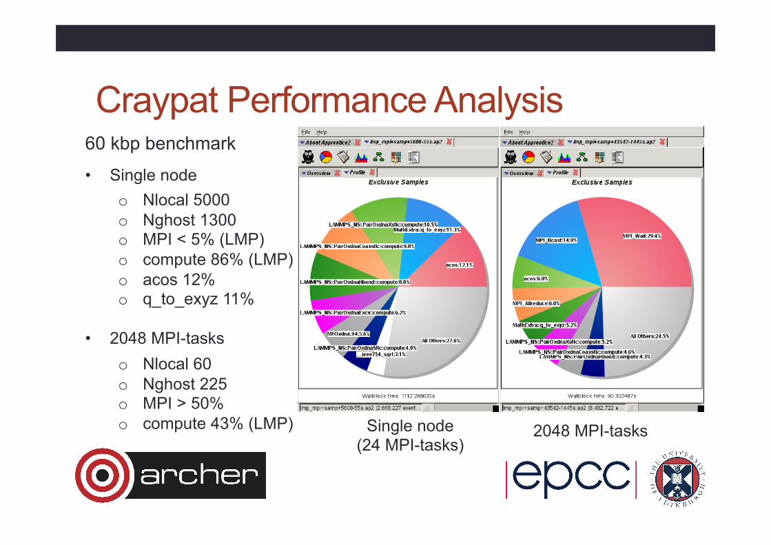
Craypat Performance Analysis 60 kbp benchmark

•  Single node o  Nlocal 5000 o  Nghost 1300 o  MPI < 5% (LMP) o  compute 86% (LMP) o  acos 12% o  q_to_exyz 11%

•  2048 MPI-tasks o  Nlocal 60 o  Nghost 225 o  MPI > 50% o  compute 43% (LMP) Single node

(24 MPI-tasks) 2048 MPI-tasks

Craypat Performance Analysis

Single node (24 MPI-tasks)

2048 MPI-tasks

960 kbp benchmark

•  Single node o  Nlocal 80000 o  Nghost 8300 o  MPI < 3% o  compute 88% (LMP) o  acos 12% o  q_to_exyz 12%

•  2048 MPI-tasks o  Nlocal 940 o  Nghost 480 o  MPI < 13% o  compute 82% (LMP)

Applications

Stand displacement DNA tetrahedra

DNA tiles

Liquid-crystalline states of DNA

DNA gel

b)

c)a)

DNA nanostructures

Code Distribution •  LAMMPS version via CCPForge o  https://ccpforge.cse.rl.ac.uk/gf

o  Project: Coarse-Grained DNA Simulation (cgdna) o  Anonymous subversion access

svn checkout https://ccpforge.cse.rl.ac.uk/svn/cgdna

•  In the near future also as LAMMPS USER-package with extended documentation

•  Standalone version from https://dna.physics.ox.ac.uk

http://www.archer.ac.uk/training/ •  Face-to-face courses

•  timetable, information and registration •  material from all past courses

• Virtual tutorials & webinars •  https://www.archer.ac.uk/training/virtual/ •  timetable plus slides and recordings •  please leave feedback on previous tutorials after viewing material

Goodbye!

Thanks for attending

Please leave feedback at: www.archer.ac.uk/training/feedback/online-course-feedback.php