WEKA Explorer User Guide

for Version 3-5-5

Richard Kirkby

Eibe Frank

Peter Reutemann

January 26, 2007

c©2002-2006 University of Waikato

Contents

1 Launching WEKA 2

2 The WEKA Explorer 42.1 Section Tabs . . . . . . . . . . . . . . . . . . . . . . . . . . . . . 42.2 Status Box . . . . . . . . . . . . . . . . . . . . . . . . . . . . . . 42.3 Log Button . . . . . . . . . . . . . . . . . . . . . . . . . . . . . . 42.4 WEKA Status Icon . . . . . . . . . . . . . . . . . . . . . . . . . . 5

3 Preprocessing 63.1 Loading Data . . . . . . . . . . . . . . . . . . . . . . . . . . . . . 63.2 The Current Relation . . . . . . . . . . . . . . . . . . . . . . . . 63.3 Working With Attributes . . . . . . . . . . . . . . . . . . . . . . 73.4 Working With Filters . . . . . . . . . . . . . . . . . . . . . . . . 8

4 Classification 104.1 Selecting a Classifier . . . . . . . . . . . . . . . . . . . . . . . . . 104.2 Test Options . . . . . . . . . . . . . . . . . . . . . . . . . . . . . 104.3 The Class Attribute . . . . . . . . . . . . . . . . . . . . . . . . . 114.4 Training a Classifier . . . . . . . . . . . . . . . . . . . . . . . . . 114.5 The Classifier Output Text . . . . . . . . . . . . . . . . . . . . . 114.6 The Result List . . . . . . . . . . . . . . . . . . . . . . . . . . . . 12

5 Clustering 145.1 Selecting a Clusterer . . . . . . . . . . . . . . . . . . . . . . . . . 145.2 Cluster Modes . . . . . . . . . . . . . . . . . . . . . . . . . . . . 145.3 Ignoring Attributes . . . . . . . . . . . . . . . . . . . . . . . . . . 145.4 Learning Clusters . . . . . . . . . . . . . . . . . . . . . . . . . . . 15

6 Associating 166.1 Setting Up . . . . . . . . . . . . . . . . . . . . . . . . . . . . . . . 166.2 Learning Associations . . . . . . . . . . . . . . . . . . . . . . . . 16

7 Selecting Attributes 177.1 Searching and Evaluating . . . . . . . . . . . . . . . . . . . . . . 177.2 Options . . . . . . . . . . . . . . . . . . . . . . . . . . . . . . . . 177.3 Performing Selection . . . . . . . . . . . . . . . . . . . . . . . . . 17

8 Visualizing 198.1 The scatter plot matrix . . . . . . . . . . . . . . . . . . . . . . . 198.2 Selecting an individual 2D scatter plot . . . . . . . . . . . . . . . 198.3 Selecting Instances . . . . . . . . . . . . . . . . . . . . . . . . . . 20

1

1 Launching WEKA

The new menu-driven GUI in WEKA (class weka.gui.Main) succeeds the oldGUI Chooser (class weka.gui.GUIChooser). Its MDI (“multiple document in-terface”) appearance makes it easier to keep track of all the open windows.

The menu consists of six sections:

1. Program

• LogWindow Opens a log window that captures all that is printedto stdout or stderr. Useful for environments like MS Windows,where WEKA is not started from a terminal.

• Exit Closes WEKA.

2. Applications Lists the main applications within WEKA.

• Explorer An environment for exploring data with WEKA (therest of this documentation deals with this application in moredetail).

• Experimenter An environment for performing experiments andconducting statistical tests between learning schemes.

• KnowledgeFlow This environment supports essentially the samefunctions as the Explorer but with a drag-and-drop interface. Oneadvantage is that it supports incremental learning.

• SimpleCLI Provides a simple command-line interface that allowsdirect execution of WEKA commands for operating systems thatdo not provide their own command line interface.

3. Tools Other useful applications.

• ArffViewer An MDI application for viewing ARFF files inspreadsheet format.

• SqlViewer represents an SQL worksheet, for querying databasesvia JDBC.

• EnsembleLibrary An interface for generating setups for Ensem-ble Selection [5].

4. Visualization Ways of visualizing data with WEKA.

• Plot For plotting a 2D plot of a dataset.

• ROC Displays a previously saved ROC curve.

2

• TreeVisualizer For displaying directed graphs, e.g., a decisiontree.

• GraphVisualizer Visualizes XML BIF or DOT format graphs,e.g., for Bayesian networks.

• BoundaryVisualizer Allows the visualization of classifier deci-sion boundaries in two dimensions.

5. Windows All open windows are listed here.

• Minimize Minimizes all current windows.

• Restore Restores all minimized windows again.

6. Help Online resources for WEKA can be found here.

• Weka homepage Opens a browser window with WEKA’s home-page.

• Online documentation Directs to the WekaDoc Wiki [4].

• HOWTOs, code snippets, etc. The general WekaWiki [3], con-taining lots of examples and HOWTOs around the development anduse of WEKA.

• Weka on Sourceforge WEKA’s project homepage on Sourceforge.net.

• SystemInfo Lists some internals about the Java/WEKA environ-ment, e.g., the CLASSPATH.

• About The infamous “About” box.

If you launch WEKA from a terminal window, some text begins scrolling inthe terminal. Ignore this text unless something goes wrong, in which case it canhelp in tracking down the cause (the LogWindow displays that information aswell).

This User Manual, which is also available online on the WekaDoc Wiki [4],focuses on using the Explorer but does not explain the individual data pre-processing tools and learning algorithms in WEKA. For more information onthe various filters and learning methods in WEKA, see the book Data Mining

[2].

3

2 The WEKA Explorer

2.1 Section Tabs

At the very top of the window, just below the title bar, is a row of tabs. Whenthe Explorer is first started only the first tab is active; the others are greyedout. This is because it is necessary to open (and potentially pre-process) a dataset before starting to explore the data.

The tabs are as follows:

1. Preprocess. Choose and modify the data being acted on.

2. Classify. Train and test learning schemes that classify or perform regres-sion.

3. Cluster. Learn clusters for the data.

4. Associate. Learn association rules for the data.

5. Select attributes. Select the most relevant attributes in the data.

6. Visualize. View an interactive 2D plot of the data.

Once the tabs are active, clicking on them flicks between different screens, onwhich the respective actions can be performed. The bottom area of the window(including the status box, the log button, and the Weka bird) stays visibleregardless of which section you are in.

2.2 Status Box

The status box appears at the very bottom of the window. It displays messagesthat keep you informed about what’s going on. For example, if the Explorer isbusy loading a file, the status box will say that.

TIP—right-clicking the mouse anywhere inside the status box brings up alittle menu. The menu gives two options:

1. Memory information. Display in the log box the amount of memoryavailable to WEKA.

2. Run garbage collector. Force the Java garbage collector to search formemory that is no longer needed and free it up, allowing more memoryfor new tasks. Note that the garbage collector is constantly running as abackground task anyway.

2.3 Log Button

Clicking on this button brings up a separate window containing a scrollable textfield. Each line of text is stamped with the time it was entered into the log. Asyou perform actions in WEKA, the log keeps a record of what has happened.For people using the command line or the SimpleCLI, the log now also containsthe full setup strings for classification, clustering, attribute selection, etc., sothat it is possible to copy/paste them elsewhere. Options for dataset(s) and, ifapplicable, the class attribute still have to be provided by the user (e.g., -t forclassifiers or -i and -o for filters).

4

2.4 WEKA Status Icon

To the right of the status box is the WEKA status icon. When no processes arerunning, the bird sits down and takes a nap. The number beside the × symbolgives the number of concurrent processes running. When the system is idle it iszero, but it increases as the number of processes increases. When any processis started, the bird gets up and starts moving around. If it’s standing but stopsmoving for a long time, it’s sick: something has gone wrong! In that case youshould restart the WEKA Explorer.

5

3 Preprocessing

3.1 Loading Data

The first four buttons at the top of the preprocess section enable you to loaddata into WEKA:

1. Open file.... Brings up a dialog box allowing you to browse for the datafile on the local file system.

2. Open URL.... Asks for a Uniform Resource Locator address for wherethe data is stored.

3. Open DB.... Reads data from a database. (Note that to make this workyou might have to edit the file in weka/experiment/DatabaseUtils.props.)

4. Generate.... Enables you to generate artificial data from a variety ofDataGenerators.

Using the Open file... button you can read files in a variety of formats:WEKA’s ARFF format, CSV format, C4.5 format, or serialized Instances for-mat. ARFF files typically have a .arff extension, CSV files a .csv extension,C4.5 files a .data and .names extension, and serialized Instances objects a .bsi

extension.NB: This list of formats can be extended by adding custom file converters

to the weka.core.converters package.

3.2 The Current Relation

Once some data has been loaded, the Preprocess panel shows a variety of in-formation. The Current relation box (the “current relation” is the currentlyloaded data, which can be interpreted as a single relational table in databaseterminology) has three entries:

6

1. Relation. The name of the relation, as given in the file it was loadedfrom. Filters (described below) modify the name of a relation.

2. Instances. The number of instances (data points/records) in the data.

3. Attributes. The number of attributes (features) in the data.

3.3 Working With Attributes

Below the Current relation box is a box titled Attributes. There are fourbuttons, and beneath them is a list of the attributes in the current relation.The list has three columns:

1. No.. A number that identifies the attribute in the order they are specifiedin the data file.

2. Selection tick boxes. These allow you select which attributes are presentin the relation.

3. Name. The name of the attribute, as it was declared in the data file.

When you click on different rows in the list of attributes, the fields changein the box to the right titled Selected attribute. This box displays the char-acteristics of the currently highlighted attribute in the list:

1. Name. The name of the attribute, the same as that given in the attributelist.

2. Type. The type of attribute, most commonly Nominal or Numeric.

3. Missing. The number (and percentage) of instances in the data for whichthis attribute is missing (unspecified).

4. Distinct. The number of different values that the data contains for thisattribute.

5. Unique. The number (and percentage) of instances in the data having avalue for this attribute that no other instances have.

Below these statistics is a list showing more information about the values storedin this attribute, which differ depending on its type. If the attribute is nominal,the list consists of each possible value for the attribute along with the numberof instances that have that value. If the attribute is numeric, the list givesfour statistics describing the distribution of values in the data—the minimum,maximum, mean and standard deviation. And below these statistics there is acoloured histogram, colour-coded according to the attribute chosen as the Class

using the box above the histogram. (This box will bring up a drop-down listof available selections when clicked.) Note that only nominal Class attributeswill result in a colour-coding. Finally, after pressing the Visualize All button,histograms for all the attributes in the data are shown in a separate window.

Returning to the attribute list, to begin with all the tick boxes are unticked.They can be toggled on/off by clicking on them individually. The four buttonsabove can also be used to change the selection:

7

1. All. All boxes are ticked.

2. None. All boxes are cleared (unticked).

3. Invert. Boxes that are ticked become unticked and vice versa.

4. Pattern. Enables the user to select attributes based on a Perl 5 RegularExpression. E.g., .* id selects all attributes which name ends with id.

Once the desired attributes have been selected, they can be removed byclicking the Remove button below the list of attributes. Note that this can beundone by clicking the Undo button, which is located next to the Edit buttonin the top-right corner of the Preprocess panel.

3.4 Working With Filters

The preprocess section allows filters to be defined that transform the datain various ways. The Filter box is used to set up the filters that are required.At the left of the Filter box is a Choose button. By clicking this button it ispossible to select one of the filters in WEKA. Once a filter has been selected, itsname and options are shown in the field next to the Choose button. Clicking onthis box with the left mouse button brings up a GenericObjectEditor dialog box.A click with the right mouse button (or Alt+Shift+left click) brings up a menuwhere you can choose, either to display the properties in a GenericObjectEditordialog box, or to copy the current setup string to the clipboard.

The GenericObjectEditor Dialog Box

The GenericObjectEditor dialog box lets you configure a filter. The same kindof dialog box is used to configure other objects, such as classifiers and clusterers(see below). The fields in the window reflect the available options. Clicking onany of these gives an opportunity to alter the filters settings. For example, thesetting may take a text string, in which case you type the string into the textfield provided. Or it may give a drop-down box listing several states to choose

8

from. Or it may do something else, depending on the information required.Information on the options is provided in a tool tip if you let the mouse pointerhover of the corresponding field. More information on the filter and its optionscan be obtained by clicking on the More button in the About panel at the topof the GenericObjectEditor window.

Some objects display a brief description of what they do in an About box,along with a More button. Clicking on the More button brings up a windowdescribing what the different options do. Others have an additional button,Capabilities, which lists the types of attributes and classes the object can handle.

At the bottom of the GenericObjectEditor dialog are four buttons. The firsttwo, Open... and Save... allow object configurations to be stored for futureuse. The Cancel button backs out without remembering any changes that havebeen made. Once you are happy with the object and settings you have chosen,click OK to return to the main Explorer window.

Applying Filters

Once you have selected and configured a filter, you can apply it to the data bypressing the Apply button at the right end of the Filter panel in the Preprocesspanel. The Preprocess panel will then show the transformed data. The changecan be undone by pressing the Undo button. You can also use the Edit...button to modify your data manually in a dataset editor. Finally, the Save...button at the top right of the Preprocess panel saves the current version of therelation in file formats that can represent the relation, allowing it to be kept forfuture use.

Note: Some of the filters behave differently depending on whether a class at-tribute has been set or not (using the box above the histogram, which willbring up a drop-down list of possible selections when clicked). In particular, the“supervised filters” require a class attribute to be set, and some of the “unsu-pervised attribute filters” will skip the class attribute if one is set. Note that itis also possible to set Class to None, in which case no class is set.

9

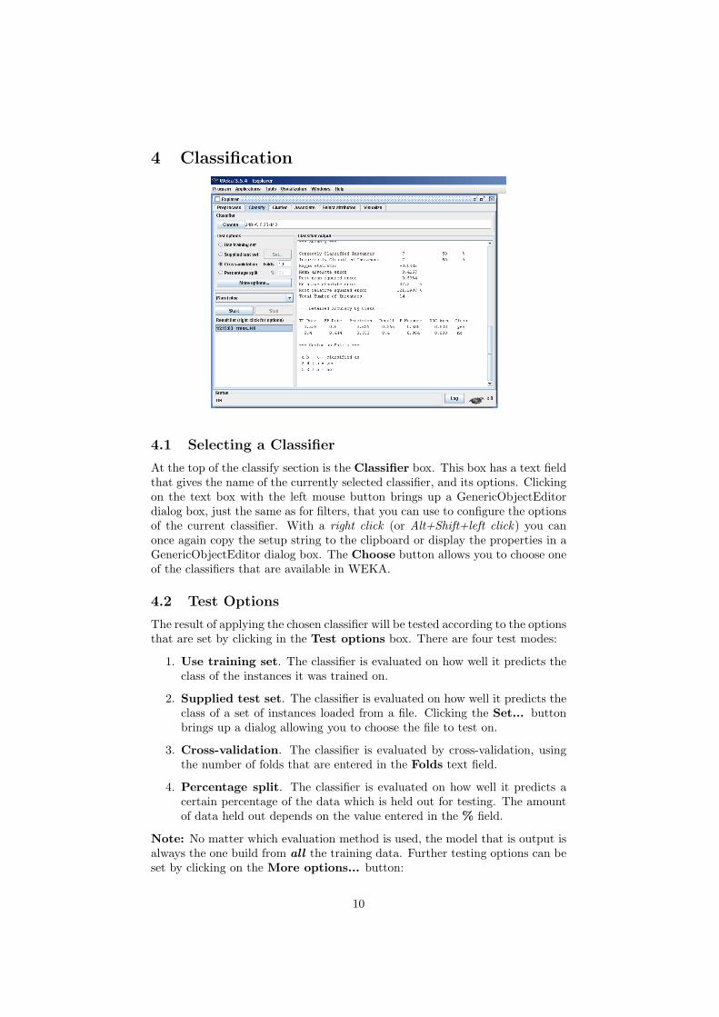
4 Classification

4.1 Selecting a Classifier

At the top of the classify section is the Classifier box. This box has a text fieldthat gives the name of the currently selected classifier, and its options. Clickingon the text box with the left mouse button brings up a GenericObjectEditordialog box, just the same as for filters, that you can use to configure the optionsof the current classifier. With a right click (or Alt+Shift+left click) you canonce again copy the setup string to the clipboard or display the properties in aGenericObjectEditor dialog box. The Choose button allows you to choose oneof the classifiers that are available in WEKA.

4.2 Test Options

The result of applying the chosen classifier will be tested according to the optionsthat are set by clicking in the Test options box. There are four test modes:

1. Use training set. The classifier is evaluated on how well it predicts theclass of the instances it was trained on.

2. Supplied test set. The classifier is evaluated on how well it predicts theclass of a set of instances loaded from a file. Clicking the Set... buttonbrings up a dialog allowing you to choose the file to test on.

3. Cross-validation. The classifier is evaluated by cross-validation, usingthe number of folds that are entered in the Folds text field.

4. Percentage split. The classifier is evaluated on how well it predicts acertain percentage of the data which is held out for testing. The amountof data held out depends on the value entered in the % field.

Note: No matter which evaluation method is used, the model that is output isalways the one build from all the training data. Further testing options can beset by clicking on the More options... button:

10

1. Output model. The classification model on the full training set is outputso that it can be viewed, visualized, etc. This option is selected by default.

2. Output per-class stats. The precision/recall and true/false statisticsfor each class are output. This option is also selected by default.

3. Output entropy evaluation measures. Entropy evaluation measuresare included in the output. This option is not selected by default.

4. Output confusion matrix. The confusion matrix of the classifier’s pre-dictions is included in the output. This option is selected by default.

5. Store predictions for visualization. The classifier’s predictions areremembered so that they can be visualized. This option is selected bydefault.

6. Output predictions. The predictions on the evaluation data are output.Note that in the case of a cross-validation the instance numbers do notcorrespond to the location in the data!

7. Cost-sensitive evaluation. The errors is evaluated with respect to acost matrix. The Set... button allows you to specify the cost matrixused.

8. Random seed for xval / % Split. This specifies the random seed usedwhen randomizing the data before it is divided up for evaluation purposes.

4.3 The Class Attribute

The classifiers in WEKA are designed to be trained to predict a single ‘class’attribute, which is the target for prediction. Some classifiers can only learnnominal classes; others can only learn numeric classes (regression problems);still others can learn both.

By default, the class is taken to be the last attribute in the data. If you wantto train a classifier to predict a different attribute, click on the box below theTest options box to bring up a drop-down list of attributes to choose from.

4.4 Training a Classifier

Once the classifier, test options and class have all been set, the learning processis started by clicking on the Start button. While the classifier is busy beingtrained, the little bird moves around. You can stop the training process at anytime by clicking on the Stop button.

When training is complete, several things happen. The Classifier outputarea to the right of the display is filled with text describing the results of trainingand testing. A new entry appears in the Result list box. We look at the resultlist below; but first we investigate the text that has been output.

4.5 The Classifier Output Text

The text in the Classifier output area has scroll bars allowing you to browsethe results. Clicking with the left mouse button into the text area, while holding

11

Alt and Shift, brings up a dialog that enables you to save the displayed outputin a variety of formats (currently, JPEG and EPS). Of course, you can also resizethe Explorer window to get a larger display area. The output is split into severalsections:

1. Run information. A list of information giving the learning scheme op-tions, relation name, instances, attributes and test mode that were in-volved in the process.

2. Classifier model (full training set). A textual representation of theclassification model that was produced on the full training data.

3. The results of the chosen test mode are broken down thus:

4. Summary. A list of statistics summarizing how accurately the classifierwas able to predict the true class of the instances under the chosen testmode.

5. Detailed Accuracy By Class. A more detailed per-class break downof the classifier’s prediction accuracy.

6. Confusion Matrix. Shows how many instances have been assigned toeach class. Elements show the number of test examples whose actual classis the row and whose predicted class is the column.

4.6 The Result List

After training several classifiers, the result list will contain several entries. Left-clicking the entries flicks back and forth between the various results that havebeen generated. Pressing Delete removes a selected entry from the results.Right-clicking an entry invokes a menu containing these items:

1. View in main window. Shows the output in the main window (just likeleft-clicking the entry).

2. View in separate window. Opens a new independent window for view-ing the results.

3. Save result buffer. Brings up a dialog allowing you to save a text filecontaining the textual output.

4. Load model. Loads a pre-trained model object from a binary file.

5. Save model. Saves a model object to a binary file. Objects are saved inJava ‘serialized object’ form.

6. Re-evaluate model on current test set. Takes the model that hasbeen built and tests its performance on the data set that has been specifiedwith the Set.. button under the Supplied test set option.

7. Visualize classifier errors. Brings up a visualization window that plotsthe results of classification. Correctly classified instances are representedby crosses, whereas incorrectly classified ones show up as squares.

12

8. Visualize tree or Visualize graph. Brings up a graphical representationof the structure of the classifier model, if possible (i.e. for decision treesor Bayesian networks). The graph visualization option only appears if aBayesian network classifier has been built. In the tree visualizer, you canbring up a menu by right-clicking a blank area, pan around by draggingthe mouse, and see the training instances at each node by clicking on it.CTRL-clicking zooms the view out, while SHIFT-dragging a box zoomsthe view in. The graph visualizer should be self-explanatory.

9. Visualize margin curve. Generates a plot illustrating the predictionmargin. The margin is defined as the difference between the probabilitypredicted for the actual class and the highest probability predicted forthe other classes. For example, boosting algorithms may achieve betterperformance on test data by increasing the margins on the training data.

10. Visualize threshold curve. Generates a plot illustrating the trade-offsin prediction that are obtained by varying the threshold value betweenclasses. For example, with the default threshold value of 0.5, the pre-dicted probability of ‘positive’ must be greater than 0.5 for the instanceto be predicted as ‘positive’. The plot can be used to visualize the pre-cision/recall trade-off, for ROC curve analysis (true positive rate vs falsepositive rate), and for other types of curves.

11. Visualize cost curve. Generates a plot that gives an explicit represen-tation of the expected cost, as described by [1].

12. Plugins. This menu item only appears if there are Explorer visualization

plugins available (by default: none). More about these plugins can befound on the WekaWiki [3].

Options are greyed out if they do not apply to the specific set of results.

13

5 Clustering

5.1 Selecting a Clusterer

By now you will be familiar with the process of selecting and configuring objects.Clicking on the clustering scheme listed in the Clusterer box at the top of thewindow brings up a GenericObjectEditor dialog with which to choose a newclustering scheme.

5.2 Cluster Modes

The Cluster mode box is used to choose what to cluster and how to evaluatethe results. The first three options are the same as for classification: Usetraining set, Supplied test set and Percentage split (Section 4.1)—exceptthat now the data is assigned to clusters instead of trying to predict a specificclass. The fourth mode, Classes to clusters evaluation, compares how wellthe chosen clusters match up with a pre-assigned class in the data. The drop-down box below this option selects the class, just as in the Classify panel.

An additional option in the Cluster mode box, the Store clusters forvisualization tick box, determines whether or not it will be possible to visualizethe clusters once training is complete. When dealing with datasets that are solarge that memory becomes a problem it may be helpful to disable this option.

5.3 Ignoring Attributes

Often, some attributes in the data should be ignored when clustering. TheIgnore attributes button brings up a small window that allows you to selectwhich attributes are ignored. Clicking on an attribute in the window highlightsit, holding down the SHIFT key selects a range of consecutive attributes, andholding down CTRL toggles individual attributes on and off. To cancel theselection, back out with the Cancel button. To activate it, click the Selectbutton. The next time clustering is invoked, the selected attributes are ignored.

14

5.4 Learning Clusters

The Cluster section, like the Classify section, has Start/Stop buttons, aresult text area and a result list. These all behave just like their classifica-tion counterparts. Right-clicking an entry in the result list brings up a similarmenu, except that it shows only two visualization options: Visualize clusterassignments and Visualize tree. The latter is grayed out when it is notapplicable.

15

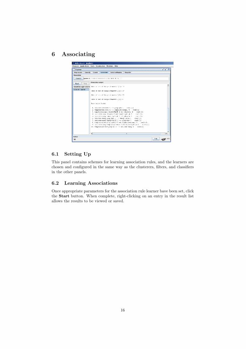
6 Associating

6.1 Setting Up

This panel contains schemes for learning association rules, and the learners arechosen and configured in the same way as the clusterers, filters, and classifiersin the other panels.

6.2 Learning Associations

Once appropriate parameters for the association rule learner bave been set, clickthe Start button. When complete, right-clicking on an entry in the result listallows the results to be viewed or saved.

16

7 Selecting Attributes

7.1 Searching and Evaluating

Attribute selection involves searching through all possible combinations of at-tributes in the data to find which subset of attributes works best for prediction.To do this, two objects must be set up: an attribute evaluator and a searchmethod. The evaluator determines what method is used to assign a worth toeach subset of attributes. The search method determines what style of searchis performed.

7.2 Options

The Attribute Selection Mode box has two options:

1. Use full training set. The worth of the attribute subset is determinedusing the full set of training data.

2. Cross-validation. The worth of the attribute subset is determined by aprocess of cross-validation. The Fold and Seed fields set the number offolds to use and the random seed used when shuffling the data.

As with Classify (Section 4.1), there is a drop-down box that can be used tospecify which attribute to treat as the class.

7.3 Performing Selection

Clicking Start starts running the attribute selection process. When it is fin-ished, the results are output into the result area, and an entry is added tothe result list. Right-clicking on the result list gives several options. The firstthree, (View in main window, View in separate window and Save resultbuffer), are the same as for the classify panel. It is also possible to Visualize

17

reduced data, or if you have used an attribute transformer such as Principal-Components, Visualize transformed data. The reduced/transformed datacan be saved to a file with the Save reduced data... or Save transformeddata... option.

In case one wants to reduce/transform a training and a test at the same timeand not use the AttributeSelectedClassifier from the classifier panel, it is bestto use the AttributeSelection filter (a supervised attribute filter) in batch mode(’-b’) from the command line or in the SimpleCLI. The batch mode allows oneto specify an additional input and output file pair (options -r and -s), that isprocessed with the filter setup that was determined based on the training data(specified by options -i and -o).

Here is an example for a Unix/Linux bash:

java weka.filters.supervised.attribute.AttributeSelection \

-E "weka.attributeSelection.CfsSubsetEval " \

-S "weka.attributeSelection.BestFirst -D 1 -N 5" \

-b \

-i <input1.arff> \

-o <output1.arff> \

-r <input2.arff> \

-s <output2.arff>

Notes:

• The “backslashes” at the end of each line tell the bash that the commandis not finished yet. Using the SimpleCLI one has to use this command inone line without the backslashes.

• It is assumed that WEKA is available in the CLASSPATH, otherwise onehas to use the -classpath option.

• The full filter setup is output in the log, as well as the setup for runningregular attribute selection.

18

8 Visualizing

WEKA’s visualization section allows you to visualize 2D plots of the currentrelation.

8.1 The scatter plot matrix

When you select the Visualize panel, it shows a scatter plot matrix for allthe attributes, colour coded according to the currently selected class. It ispossible to change the size of each individual 2D plot and the point size, and torandomly jitter the data (to uncover obscured points). It also possible to changethe attribute used to colour the plots, to select only a subset of attributes forinclusion in the scatter plot matrix, and to sub sample the data. Note thatchanges will only come into effect once the Update button has been pressed.

8.2 Selecting an individual 2D scatter plot

When you click on a cell in the scatter plot matrix, this will bring up a separatewindow with a visualization of the scatter plot you selected. (We describedabove how to visualize particular results in a separate window—for example,classifier errors—the same visualization controls are used here.)

Data points are plotted in the main area of the window. At the top are twodrop-down list buttons for selecting the axes to plot. The one on the left showswhich attribute is used for the x-axis; the one on the right shows which is usedfor the y-axis.

Beneath the x-axis selector is a drop-down list for choosing the colour scheme.This allows you to colour the points based on the attribute selected. Below theplot area, a legend describes what values the colours correspond to. If the valuesare discrete, you can modify the colour used for each one by clicking on themand making an appropriate selection in the window that pops up.

To the right of the plot area is a series of horizontal strips. Each striprepresents an attribute, and the dots within it show the distribution of values

19

of the attribute. These values are randomly scattered vertically to help you seeconcentrations of points. You can choose what axes are used in the main graphby clicking on these strips. Left-clicking an attribute strip changes the x-axisto that attribute, whereas right-clicking changes the y-axis. The ‘X’ and ‘Y’written beside the strips shows what the current axes are (‘B’ is used for ‘bothX and Y’).

Above the attribute strips is a slider labelled Jitter, which is a randomdisplacement given to all points in the plot. Dragging it to the right increases theamount of jitter, which is useful for spotting concentrations of points. Withoutjitter, a million instances at the same point would look no different to just asingle lonely instance.

8.3 Selecting Instances

There may be situations where it is helpful to select a subset of the data us-ing the visualization tool. (A special case of this is the UserClassifier in theClassify panel, which lets you build your own classifier by interactively selectinginstances.)

Below the y-axis selector button is a drop-down list button for choosing aselection method. A group of data points can be selected in four ways:

1. Select Instance. Clicking on an individual data point brings up a windowlisting its attributes. If more than one point appears at the same location,more than one set of attributes is shown.

2. Rectangle. You can create a rectangle, by dragging, that selects thepoints inside it.

3. Polygon. You can build a free-form polygon that selects the points insideit. Left-click to add vertices to the polygon, right-click to complete it. Thepolygon will always be closed off by connecting the first point to the last.

4. Polyline. You can build a polyline that distinguishes the points on oneside from those on the other. Left-click to add vertices to the polyline,right-click to finish. The resulting shape is open (as opposed to a polygon,which is always closed).

Once an area of the plot has been selected using Rectangle, Polygon orPolyline, it turns grey. At this point, clicking the Submit button removes allinstances from the plot except those within the grey selection area. Clicking onthe Clear button erases the selected area without affecting the graph.

Once any points have been removed from the graph, the Submit buttonchanges to a Reset button. This button undoes all previous removals andreturns you to the original graph with all points included. Finally, clicking theSave button allows you to save the currently visible instances to a new ARFFfile.

20

References

[1] Drummond, C. and Holte, R. (2000) Explicitly representing expectedcost: An alternative to ROC representation. Proceedings of the Sixth

ACM SIGKDD International Conference on Knowledge Discovery and

Data Mining. Publishers, San Mateo, CA.

[2] Witten, I.H. and Frank, E. (2005) Data Mining: Practical machine learn-

ing tools and techniques. 2nd edition Morgan Kaufmann, San Francisco.

[3] WekaWiki – http://weka.sourceforge.net/wiki/

[4] WekaDoc – http://weka.sourceforge.net/wekadoc/

[5] Ensemble Selection on WekaDoc –http://weka.sourceforge.net/wekadoc/index.php/en:Ensemble Selection

21