J Sci ComputDOI 10.1007/s10915-017-0421-z

Weighted Nonlocal Laplacian on Interpolation fromSparse Data

Zuoqiang Shi1 · Stanley Osher2 · Wei Zhu2

Received: 15 January 2017 / Revised: 14 March 2017 / Accepted: 18 March 2017© Springer Science+Business Media New York 2017

Abstract Inspired by the nonlocal methods in image processing and the point integralmethod, we introduce a novel weighted nonlocal Laplacian method to compute a continuousinterpolation function on a point cloud in high dimensional space. The numerical results insemi-supervised learning and image inpainting show that the weighted nonlocal Laplacianis a reliable and efficient interpolation method. In addition, it is fast and easy to implement.

Keywords Graph Laplacian · Nonlocal methods · Point cloud · Weighted nonlocalLaplacian

Mathematics Subject Classification 65D05 · 65D25 · 41A05

1 Introduction

In this paper, we consider interpolation on a point cloud in high dimensional space. Thisis a fundamental problem in many data analysis problems and machine learning. Let P ={ p1, . . . , pn} be a set of points in R

d and S = {s1, . . . , sm} be a subset of P . Let u be afunction on the point set P and the value of u on S ⊂ P is given as a function g over S, i.e.

This research was supported by DOE-SC0013838 and NSF DMS-1118971. Zuoqiang Shi was partiallysupported by NSFC Grants 11371220, 11671005.

B Zuoqiang Shizqshi@mail.tsinghua.edu.cn

Stanley Oshersjo@math.ucla.edu

Wei Zhuweizhu731@math.ucla.edu

1 Yau Mathematical Sciences Center, Tsinghua University, Beijing 100084, China

2 Department of Mathematics, University of California, Los Angeles, CA 90095, USA

123

J Sci Comput

u(s) = g(s), ∀s ∈ S. The goal of the interpolation is to find the function u on P with thegiven values on S.

Since the point set P is unstructured in high dimensional space, traditional interpolationmethods do not apply. One model which is widely used in many applications is to minimizethe following energy functional,

J (u) = 1

2

∑

x, y∈P

w(x, y)(u(x) − u( y))2, (1.1)

with the constraintu(x) = g(x), x ∈ S. (1.2)

here w(x, y) is a given weight function. One often used weight is the Gaussian weight,

w(x, y) = exp(−‖x− y‖2σ 2 ), σ is a parameter, ‖ · ‖ is the Euclidean norm in Rd .

It is easy to derive the Euler–Lagrange equation of the above optimization problem, whichis given as follows,

⎧⎨

⎩

∑

y∈P

(w(x, y) + w( y, x))(u(x) − u( y)) = 0, x ∈ P\S,

u(x) = g(x), x ∈ S.

(1.3)

If the weight function w(x, y) is symmetric, above equation can be simplified further to be∑

y∈P

w(x, y)(u(x) − u( y)) = 0.

This is just the well known nonlocal Laplacian which is widely used in nonlocal methods ofimage processing [1,2,7,8]. It is also called graph Laplacian in graph and machine learningliterature [4,19]. In the rest of the paper, we use the abbreviation, GL, to denote this approach.

Recently, it was observed that the solution given by the graph Laplacian is not continuousat the sample points, S, especially when the sample rate, |S|/|P|, is low [15]. Consider asimple 1D example. Let P be the union of 5000 randomly sampled points over the interval(0, 2) and we label 6 points in P . Points 0, 1, 2 are in the labeled set S and the other 3 pointsare selected at random. The solution given by the graph Laplacian, (1.3) is shown in Fig.1. Clearly, the labeled points are not consistent with the function computed by the graphLaplacian. In other words, the graph Laplacian actually does not interpolate the given values.

It was also shown that the discontinuity is due to the fact that one important boundaryterm is dropped in evaluating the graph Laplacian. Consider the harmonic extension in thecontinuous formwhich is formulated as aLaplace–Beltrami equationwithDirichlet boundarycondition on manifold M, {

�Mu(x) = 0, x ∈ M,

u(x) = g(x), x ∈ ∂M,(1.4)

In the point integral method [9,10,13,14], it is observed that the Laplace–Beltrami equa-tion �Mu(x) = 0 can be approximated by the following integral equation.

1

t

∫

M(u(x) − u( y))Rt (x, y)d y − 2

∫

∂M

∂u( y)∂n

R̄t (x, y)dτ y = 0, (1.5)

where Rt (x, y) = R(−|x− y|2

4t

), R̄t (x, y) = R̄

(−|x− y|2

4t

)and d

ds R̄(s) = −R(s). If

R(s) = exp(−s), R̄ = R and Rt (x, y)becomes aGaussianweight function.n is the outwardsnormal of the boundary ∂M.

123

J Sci Comput

Fig. 1 Solution given by graphLaplacian in 1D examples. Blueline interpolation function givenby graph Laplacian; red circlesgiven values at label set S (Colorfigure online)

0 0.2 0.4 0.6 0.8 1 1.2 1.4 1.6 1.8 2−1

−0.5

0

0.5

1

1.5

2

2.5Graph Laplacian

Comparing the above integral equation (1.5) and the equation in the graph Laplacian(1.3), we can clearly see that the boundary term in (1.5) is dropped in the graph Laplacian.However, this boundary term is not small and neglecting it causes trouble. To get an reasonableinterpolation, we need to include the boundary term. This is the idea of the point integralmethod. To deal with the boundary term in (1.5), a Robin boundary condition is used toapproximate the Dirichlet boundary condition,

u(x) + μ∂u(x)

∂n= g(x), x ∈ ∂M, (1.6)

where 0 < μ � 1 is a small parameter.Substituting above Robin boundary condition to the integral equation (1.5), we get an

integral equation to approximate the Dirichlet problem (1.4),

1

t

∫

M(u(x) − u( y))Rt (x, y)d y − 2

μ

∫

∂MR̄t (x, y)(g( y) − u( y))dτ y = 0.

The corresponding discrete equations are

∑

y∈P

Rt (x, y)(u(x) − u( y)) + 2

μ

∑

y∈SR̄t (x, y)(u( y) − g( y)) = 0, x ∈ P, (1.7)

The point integral method has been shown to give consistent solutions [9,14,15]. The inter-polation algorithm based on the point integral method has been applied to image processingproblems and gives promising results [12].

Equation (1.7) is not symmetric, which makes the numerical solver not very efficient. Themain contribution of this paper is to propose a novel interpolation algorithm, the weightednonlocal Laplacian, which preserves the symmetry of the original Laplace operator. The keyobservation in the weighted nonlocal Laplacian is that we need to modify the energy function(1.1) to add a weight to balance the energy on the labeled and unlabeled sets.

123

J Sci Comput

minu

∑

x∈P\S

⎛

⎝∑

y∈P

w(x, y)(u(x) − u( y))2

⎞

⎠ + |P||S|

∑

x∈S

⎛

⎝∑

y∈P

w(x, y)(u(x) − u( y))2

⎞

⎠ ,

with the constraint

u(x) = g(x), x ∈ S.

|P|, |S| are the number of points in P and S, respectively. When the sample rate, |S|/|P|,is high, the weighted nonlocal Laplacian becomes the classical graph Laplacian. When thesample rate is low, the large weight in weighted nonlocal Laplacian forces the solution closeto the given values near the labeled set, such that the inconsistent phenomenon is removed.

We test the weighted nonlocal Laplacian on MNIST dataset and image inpainting prob-lems. The results show that the weighted nonlocal Laplacian gives better results than thegraph Laplacian, especially when the sample rate is low. The weighted nonlocal Laplacianprovides a reliable and efficient method to find reasonable interpolation on a point cloud inhigh dimensional space.

The rest of the paper is organized as follows. The weighted nonlocal Laplacian is intro-duced inSect. 2. The tests of theweighted nonlocalLaplacian onMNISTand image inpaintingare presented in Sects. 3 and 4 respectively. Some conclusions are made in Sect. 5.

2 Weighted Nonlocal Laplacian

First, we split the objective function in (1.1) to two terms, one is over the unlabeled set andthe other over the labeled set.

minu

∑

x∈P\S

⎛

⎝∑

y∈P

w(x, y)(u(x) − u( y))2

⎞

⎠ +∑

x∈S

⎛

⎝∑

y∈P

w(x, y)(u(x) − u( y))2

⎞

⎠ ,

Ifwe substitute the optimal solution into above optimization problem, for instance the solutionin the 1Dexample (Fig. 1), it is easy to check that the summation over the labeled set is actuallypretty large due to the discontinuity on the labeled set. However, when the sample rate is low,the summation over the unlabeled set actually overwhelms the summation over the labeledset. So the continuity on the labeled set is sacrificed. One simple idea to assure the continuityon the labeled set is to put a weight ahead of the summation over the labeled set.

minu

∑

x∈P\S

⎛

⎝∑

y∈P

w(x, y)(u(x) − u( y))2

⎞

⎠ + μ∑

x∈S

⎛

⎝∑

y∈P

w(x, y)(u(x) − u( y))2

⎞

⎠ ,

This is the basic idea of our approach. Since thismethod is obtained bymodifying the nonlocalLaplacian to add a weight, we call this method the weighted nonlocal Laplacian, WNLL forshort.

To balance these two terms, one natural choice of the weightμ is the inverse of the samplerate, |P|/|S|. Based on this observation, we get following optimization problem

minu

∑

x∈P\S

⎛

⎝∑

y∈P

w(x, y)(u(x) − u( y))2

⎞

⎠ + |P||S|

∑

x∈S

⎛

⎝∑

y∈P

w(x, y)(u(x) − u( y))2

⎞

⎠ ,

(2.1)

123

J Sci Comput

0 0.2 0.4 0.6 0.8 1 1.2 1.4 1.6 1.8 2−1

−0.5

0

0.5

1

1.5

2

2.5Graph Laplacian

0 0.2 0.4 0.6 0.8 1 1.2 1.4 1.6 1.8 2−1

−0.5

0

0.5

1

1.5

2

2.5Weighted Nonlocal Laplacian

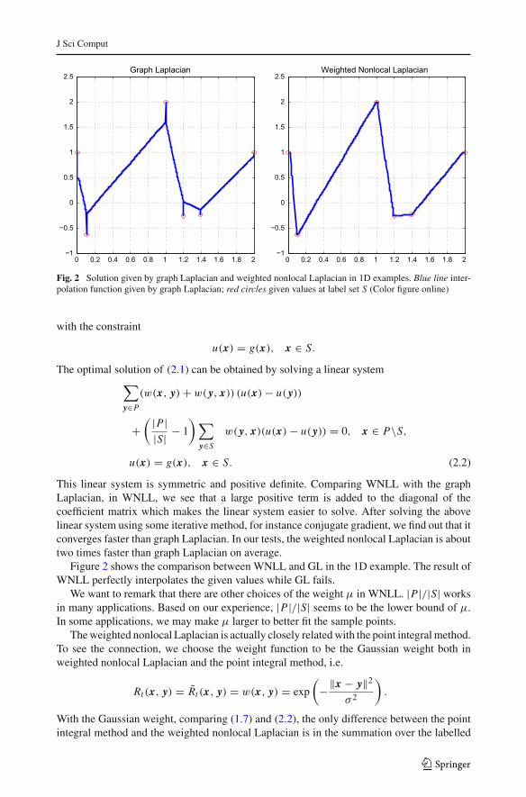
Fig. 2 Solution given by graph Laplacian and weighted nonlocal Laplacian in 1D examples. Blue line inter-polation function given by graph Laplacian; red circles given values at label set S (Color figure online)

with the constraint

u(x) = g(x), x ∈ S.

The optimal solution of (2.1) can be obtained by solving a linear system∑

y∈P

(w(x, y) + w( y, x)) (u(x) − u( y))

+( |P|

|S| − 1

) ∑

y∈Sw( y, x)(u(x) − u( y)) = 0, x ∈ P\S,

u(x) = g(x), x ∈ S. (2.2)

This linear system is symmetric and positive definite. Comparing WNLL with the graphLaplacian, in WNLL, we see that a large positive term is added to the diagonal of thecoefficient matrix which makes the linear system easier to solve. After solving the abovelinear system using some iterative method, for instance conjugate gradient, we find out that itconverges faster than graph Laplacian. In our tests, the weighted nonlocal Laplacian is abouttwo times faster than graph Laplacian on average.

Figure 2 shows the comparison between WNLL and GL in the 1D example. The result ofWNLL perfectly interpolates the given values while GL fails.

We want to remark that there are other choices of the weight μ in WNLL. |P|/|S| worksin many applications. Based on our experience, |P|/|S| seems to be the lower bound of μ.In some applications, we may make μ larger to better fit the sample points.

Theweighted nonlocal Laplacian is actually closely relatedwith the point integralmethod.To see the connection, we choose the weight function to be the Gaussian weight both inweighted nonlocal Laplacian and the point integral method, i.e.

Rt (x, y) = R̄t (x, y) = w(x, y) = exp

(−‖x − y‖2

σ 2

).

With the Gaussian weight, comparing (1.7) and (2.2), the only difference between the pointintegral method and the weighted nonlocal Laplacian is in the summation over the labelled

123

J Sci Comput

Algorithm 1 Semi-Supervised Learning

Require: A point set P = { p1, p2, . . . , pn} ⊂ Rd and a partial labeled set S = ∪l

i=1Si .Ensure: A complete label assignment L : P → {1, 2, . . . , l}for i = 1 : l doCompute φi on P , with the constraint

φi (x) = 1, x ∈ Si , φi (x) = 0, x ∈ S\Si ,end forfor (x ∈ P\S) doLabel x as following

L(x) = k, where k = arg max1≤i≤l

φi (x).

end for

set S, u( y) is changed to u(x). After this changing, the equation becomes symmetric andpositive definite which is much easier to solve. In addition to the symmetry, it is easy to showthat the weighted nonlocal Laplacian also preserves the maximum principle of the originalLaplace–Beltrami operator, which is important in some applications.

3 Semi-Supervised Learning

In this section, we briefly describe the algorithm of semi-supervised learning based on thatproposed by Zhu et al. [19]. We plug into the algorithm the aforementioned approach forweighted nonlocal Laplacian, and apply them to thewell-knownMNISTdataset, and comparetheir performances.

Assume we are given a point set P = { p1, p2, . . . , pn} ⊂ Rd , and some labels

{1, 2, . . . , l}. A subset S ⊂ P is labeled,

S =l⋃

i=1

Si ,

Si is the labeled set with label i . In a typical setting, the size of the labeled set S is muchsmaller than the size of the data set P . The purpose of the semi-supervised learning is toextend the label assignment to the entire P , namely, infer the labels for the unlabeled points.The algorithm is summarized in Algorithm 1.

In Algorithm 1, we use both graph Laplacian and weighted nonlocal Laplacian to computeφi respectively. Inweighted nonlocal Laplacian,φi is obtained by solving the following linearsystem

∑

y∈P

(w(x, y) + w( y, x)) (φi (x) − φi ( y))

+( |P|

|S| − 1

) ∑

y∈Sw( y, x)(φi (x) − φi ( y)) = 0, x ∈ P\S,

φi (x) = 1, x ∈ Si , φi (x) = 0, x ∈ S\Si .

123

J Sci Comput

Fig. 3 Some images in MNISTdataset. The whole datasetcontains 70,000 28 × 28 grayscale digit images

Table 1 Accuracy of weighted nonlocal Laplacian and graph Laplacian in the test of MNIST

100/70,000 70/70,000 50/70,000

WNLL (%) GL (%) WNLL (%) GL (%) WNLL (%) GL (%)

91.83 74.56 84.31 29.67 79.20 33.93

89.20 58.16 87.74 42.29 78.66 21.12

93.13 62.98 83.19 37.02 71.29 24.50

90.43 41.27 91.08 12.57 71.92 29.79

92.27 44.57 84.74 35.15 80.92 37.50

In graph Laplacian, we need to solve∑

y∈P

(w(x, y) + w( y, x)) (φi (x) − φi ( y)) = 0, x ∈ P\S,

φi (x) = 1, x ∈ Si , φi (x) = 0, x ∈ S\Si .We test Algorithm 1 onMNIST dataset of handwritten digits [3]. MNIST dataset contains

70,000 28 × 28 gray scale digit images (Fig. 3). We view digits 0 ∼ 9 as ten classes. Eachimage can be seen as a point in 784-dimensional Euclidean space. The weight functionw(x, y) is constructed as following

w(x, y) = exp

(−‖x − y‖2

σ(x)2

)(3.1)

σ(x) is chosen to be the distance between x and its 20th nearest neighbor, Tomake the weightmatrix sparse, the weight is truncated to the 50 nearest neighbors.

In our test, we label 100, 70 and 50 images respectively. The labeled images are selectedat random in 70,000 images. For each case, we do 5 independent tests and the results areshown in Table 1. It is quite clear that WNLL has a better performance than GL. The averageaccuracy of WNLL is much higher than that of GL. In addition, WNLL is more stablethan GL. The fluctuation of GL in different tests is much higher. Due to the inconsistency,in GL, the values in the labeled points are not well spread on to the unlabeled points. Onmany unlabeled points, the function φi is actually close to 1/2. This makes the classificationsensitive to the distribution of the labeled points.

123

J Sci Comput

As for the computational time, in our tests, WNLL takes about half the time of GL onaverage, 15 versus 29s (not including the time to construct the weight), with Matlab code ina laptop equipped with CPU Intel i7-4900 2.8 GHz. In WNLL, a positive term is added tothe diagonal of the coefficient matrix which makes conjugate gradient converge faster.

As a remark, in this paper, we do not intend to give a state-of-the-art method in semi-supervised learning. We just use this example to test the weighted nonlocal Laplacian.

4 Image Inpainting

In this section, we apply theweighted nonlocal Laplacian to the reconstruction of subsampledimages. To apply the weighted nonlocal Laplacian, first, we construct a point cloud from agiven image by taking patches. We consider a discrete image f ∈ R

m×n . For any (i, j) ∈{1, 2, . . . ,m} × {1, 2, . . . , n}, we define a patch pi j ( f ) as a 2D piece of size s1 × s2 of theoriginal image f , and the pixel (i, j) is the center of the rectangle of size s1 × s2. The patchset P( f ) is defined as the collection of all patches:

P( f ) = {pi j ( f ) : (i, j) ∈ {1, 2, . . . ,m} × {1, 2, . . . , n}} ⊂ Rd , d = s1 × s2.

To get the patches near the boundary, we extend the images by mirror reflection. For a givenimage f , the patch set P( f ) gives a point cloud in R

d with d = s1 × s2. We also define afunction u on P( f ). At each patch, the value of u is defined to be the intensity of image fat the central pixel of the patch, i.e.

u(pi j ( f )) = f (i, j),

where f (i, j) is the intensity of image f at pixel (i, j).Now, we subsample the image f in the subsample domain� ⊂ {(i, j) : 1 ≤ i ≤ m, 1 ≤

j ≤ n}. The problem is to recover the original image f from the subsamples f |�. Thisproblem can be transferred to interpolation of function u in the patch set P( f ) with u isgiven in S ⊂ P( f ), S = {pi j ( f ) : (i, j) ∈ �}. Notice that the patch set P( f ) is not known,we need to update the patch set iteratively from the recovered image. Summarizing this idea,we get an algorithm to reconstruct the subsampled image which is stated in Algorithm 2.

Algorithm 2 Subsample image restorationRequire: A subsample image f |�.Ensure: A recovered image u.

Generate initial image u0.

while not converge do

1. Generate patch set P(un) from current image un and get corresponding labeled set Sn ⊂ P(un).

2. Compute the weight function wn(x, y) for x, y ∈ P(un).

3. Update the image by computing un+1 on P(un), with the constraint

un+1(x) = f (x), x ∈ Sn .

4. n ← n + 1.end whileu = un .

123

J Sci Comput

There are different methods to compute un+1 on P(un) in Algorithm 2. In this paper,we use weighted nonlocal Laplacian and graph Laplacian to compute un+1. In the weightednonlocal Laplacian, we need to solve the following linear system

∑

y∈P(un)

(wn(x, y) + wn( y, x))(un+1(x) − un+1( y)

)

+(mn

|�| − 1

) ∑

y∈Snwn( y, x)(un+1(x) − un+1( y)) = 0, x ∈ P(un)\Sn,

un+1(x) = f (x), x ∈ Sn .

While in the graph Laplacian, we solve the other linear system,∑

y∈P(un)

(wn(x, y) + wn( y, x))(un+1(x) − un+1( y)

) = 0, x ∈ P(un)\Sn,

un+1(x) = f (x), x ∈ Sn .

Actually, Algorithm 2 with graph Laplacian is just a nonlocal method in image processing[1,8]. In nonlocal methods, people try to minimize energy functions such as

minu

m∑

i=1

n∑

j=1

|∇wu(i, j)|2,

with the constraint

u(i, j) = f (i, j), (i, j) ∈ �.

∇wu(i, j) is the nonlocal gradient which is defined as

∇wu(i, j) = √w(i, j; i ′, j ′)(u(i ′, j ′) − u(i, j)), 1 ≤ i, i ′ ≤ m, 1 ≤ j, j ′ ≤ n.

w(i, j; i ′, j ′) is the weight from pixel (i, j) to pixel (i ′, j ′),

w(i, j; i ′, j ′) = exp

(d( f (i, j), f (i ′, j ′))

σ 2

)

d( f (i, j), f (i ′, j ′)) is the patch distance in image f ,

d( f (i, j), f (i ′, j ′)) =h1∑

k=−h1

h2∑

l=−h2

χ(k, l)| f (i + k, j + l) − f (i ′ + k, j ′ + l)|2

χ is often chosen to be 1 or a Gaussian, h1, h2 are half sizes of the patch. It is easy to checkthat the above nonlocal method is the same as solving the graph Laplacian on the patch set.If the weight w is updated iteratively, we get Algorithm 2 with the graph Laplacian. Next,we will show that this method has inconsistent results, and we can use the weighted graphLaplacian to address this issue.

In our calculations below, we take the weight w(x, y) as following:

w(x, y) = exp

(−‖x − y‖2

σ(x)2

).

σ (x) is chosen to be the distance between x and its 20th nearest neighbor, Tomake the weightmatrix sparse, the weight is truncated to the 50 nearest neighbors. The patch size is 11× 11.For each patch, the nearest neighbors are obtained by using an approximate nearest neighbor

123

J Sci Comput

Fig. 4 Test of image restoration on image of Barbara. a original image; b 1% subsample; c result of GL; dresult of WNLL

(ANN) search algorithm. We use a k-d tree approach as well as an ANN search algorithm toreduce the computational cost. The linear system in weighted nonlocal Laplacian and graphLaplacian is solved by the conjugate gradient method.

PSNR defined as following is used to measure the accuracy of the results

PSNR( f, f ∗) = −20 log10(‖ f − f ∗‖/255) (4.1)

where f ∗ is the ground truth.First, we run a simple test to see the performance of weighted nonlocal Laplacian and

graph Laplacian. In this test, the patch set is constructed using the original image, Fig. 4a.The original image is subsampled at random, only keeping 1% pixels. Since the patch set isexact, we do not update the patch set and only run WNLL and GL once to get the recoveredimage.

The results of WNLL and GL are shown in Fig. 4c, d respectively. Obviously, the resultof WNLL is much better. To have a closer look at of the recovery, Fig. 5 shows the zoomedin image enclosed by the boxes in Fig. 4a. In Fig. 5d, there are many pixels which are notconsistent with their neighbors. Compared with the subsample image 5b, it is easy to checkthat these pixels are actually the retained pixels. The reason is that in graph Laplacian a non-negligible boundary term is dropped [14,15]. On the contrary, in the result of WNLL, the

123

J Sci Comput

Fig. 5 Zoomed in image in the test of image restoration on image of Barbara. a Original image; b 1%subsample; c result of GL; d result of WNLL

inconsistency disappears and the resultant recovery is much better and smoother as shownin Figs. 4d and 5d.

At the end of this section, we apply Algorithm 2 to recover the subsampled image. In thistest, we modify the patch to add the local coordinate

p̄i j ( f ) = [pi j ( f ), λ1i, λ2 j]with

λ1 = 3‖( f |�)‖∞m

, λ2 = 3‖( f |�)‖∞n

.

This semi-local patch could accelerate the iteration and give better reconstruction. The num-ber of iterations in our computation is fixed to be 10.

The initial image is obtained by filling the missing pixels with random numbers whichsatisfy a Gaussian distribution, where μ0 is the mean of f |� and σ0 is the standard deviationof f |�.

The results are shown in Fig. 6. As we can see, WNLL gives much better results than GLboth visually and numerically in PSNR. The results are comparable with those in LDMM[12] while WNLL is much faster. For the image of Barbara (256× 256), WNLL needs about1 min and LDMM needs about 20 min in a laptop equipped with CPU Intel i7-4900 2.8

123

J Sci Comput

original image 10% subsample GL WNLL

23.74 dB 26.13 dB

22.51 dB 25.21 dB

28.29 dB 31.29 dB

21.60 dB 23.05 dB

Fig. 6 Results of subsample image restoration

GHz with matlab code. In WNLL and GL, the weight update is the most computationallyexpensive part in the algorithm by taking more than 90% of the entire computational time.This part is the same in WNLL and GL. So the total time of WNLL and GL are almost same,although the time of solving the linear system is about half in WNLL, 1.7 versus 3.1 s.

5 Conclusion and Future Work

In this paper, we introduce a novel weighted nonlocal Laplacian method. The numericalresults show that weighted nonlocal Laplacian provides a reliable and efficient method tofind reasonable interpolation on a point cloud in high dimensional space.

On the other hand, it was found that with extremely low sample rate, formulation ofthe harmonic extension may fail [11,17]. In this case, we are considering minimizing L∞norm of the gradient to compute the interpolation on point cloud, i.e. solving the following

123

J Sci Comput

optimization problem

minu

⎛

⎜⎝maxx∈P

⎛

⎝∑

y∈P

w(x, y)(u(x) − u( y))2

⎞

⎠1/2

⎞

⎟⎠ ,

with the constraint

u(x) = g(x), x ∈ S.

This approach is closely related with the infinity Laplacian which has been studied a lot inthe machine learning community [5,6].

Another interesting problem is the semi-supervised learning studied in Sect. 3. In semi-supervised learning, ideally, the functions, φi , should be either 0 or 1, so they are piecewiseconstant. In this sense, minimizing the total variation should give better results [8,16,18].Based on the weighted nonlocal Laplacian, we should also add a weight to correctly enforcethe constraints on the labeled points. This idea implies the following weighted nonlocal TVmethod,

minu

∑

x∈P\S

⎛

⎝∑

y∈P

w(x, y)(u(x) − u( y))2

⎞

⎠1/2

+ |P||S|

∑

x∈S

⎛

⎝∑

y∈P

w(x, y)(u(x) − u( y))2

⎞

⎠1/2

,

with the constraint

u(x) = g(x), x ∈ S.

This seems to be a better approach than the weighted nonlocal Laplacian in the semi-supervised learning. We will explore this approach and report its performance in our futurework.

References

1. Buades, A., Coll, B., Morel, J.-M.: A review of image denoising algorithms, with a new one. MultiscaleModel. Simul. 4, 490–530 (2005)

2. Buades, A., Coll, B., Morel, J.-M.: Neighborhood filters and PDE’s. Numer. Math. 105, 1–34 (2006)3. Burges, C.J., LeCun, Y., Cortes, C.: MNIST database4. Chung, F.R.K.: Spectral Graph Theory. American Mathematical Society, Providence (1997)5. Elmoataz Abderrahim, L.Z.L.O., Xavier, Desquesnes: Nonlocal infinity Laplacian equation on graphs

with applications in image processing and machine learning. Math. Comput. Simul. 102, 153–163 (2014)6. Ghoniem, M., Elmoataz, A., Lezoray, O.: Discrete infinity harmonic functions: towards a unified inter-

polation framework on graphs. In: IEEE International Conference on Image Processing (2011)7. Gilboa, G., Osher, S.: Nonlocal linear image regularization and supervised segmentation. Multiscale

Model. Simul. 6, 595–630 (2007)8. Gilboa, G., Osher, S.: Nonlocal operators with applications to image processing.MultiscaleModel. Simul.

7, 1005–1028 (2008)9. Li, Z., Shi, Z.: A convergent point integral method for isotropic elliptic equations on point cloud. SIAM

Multiscale Model. Simul. 14, 874–905 (2016)10. Li, Z., Shi, Z., Sun, J.: Point integral method for solving Poisson-type equations on manifolds from point

clouds with convergence guarantees. arXiv:1409.262311. Nadler, B., Srebro, N., Zhou, X.: Semi-supervised learning with the graph Laplacian: the limit of infinite

unlabelled data. In: NIPS (2009)12. Osher, S., Shi, Z., Zhu, W.: Low dimensional manifold model for image processing. Technical report,

CAM report 16-04, UCLA (2016)

123

J Sci Comput

13. Shi, Z., Sun, J.: Convergence of the point integral method for Poisson equation on point cloud.arXiv:1403.2141

14. Shi, Z., Sun, J.: Convergence of the point integral method for the Poisson equationwithDirichlet boundaryon point cloud. arXiv:1312.4424

15. Shi, Z., Sun, J., Tian, M.: Harmonic extension on point cloud. arXiv:1509.0645816. Yin, K., Tai, X.-C., Osher, S.: An effective region force for some variational models for learning and

clustering. Technical report, CAM report 16-18, UCLA (2016)17. Zhou, X., Belkin, M.: Semi-supervised learning by higher order regularization. In: NIPS (2011)18. Zhu, W., Chayes, V., Tiard, A., Sanchez, S., Dahlberg, D., Kuang, D., Bertozzi, A., Osher, S., Zosso,

D.: Nonlocal total variation with primal dual algorithm and stable simplex clustering in unspervisedhyperspectral imagery analysis. Technical report, CAM report 15-44, UCLA (2015)

19. Zhu, X., Ghahramani, Z., Lafferty, J.D.: Semi-supervised learning using Gaussian fields and harmonicfunctions. In: Machine Learning, Proceedings of the Twentieth International Conference ICML 2003,21–24 Aug 2003, Washington, DC, USA, pp. 912–919 (2003)

123