Weierstraß-Institutfür Angewandte Analysis und StochastikLeibniz-Institut im Forschungsverbund Berlin e. V.

Preprint ISSN 2198-5855

Dynamics of micro-integrated external-cavity diode lasers:

simulations, analysis and experiments

Mindaugas Radziunas1, Vasile Z. Tronciu2 , Erdenetsetseg Luvsandamdin3,

Christian Kürbis 3, Andreas Wicht 3, Hans Wenzel 3

submitted: July 10, 2014

1 Weierstrass InstituteMohrenstr. 3910117 Berlin, GermanyE-Mail: Mindaugas.Radziunas@wias-berlin.de

2 Department of PhysicsTechnical University of Moldovabd. Stefan cel Mare 168Chisinau MD-2004, MoldovaE-Mail: tronciu@mail.utm.md

3 Ferdinand-Braun-Institut, Leibniz-Institut für HöchstfrequenztechnikGustav-Kirchhoff-Str. 412489 Berlin, GermanyE-Mail: erdenetsetseg.luvsandamdin@fbh-berlin.de

christian.kuerbis@fbh-berlin.deandreas.wicht@fbh-berlin.dehans.wenzel@fbh-berlin.de

No. 1981

Berlin 2014

2010 Mathematics Subject Classification. 78A60, 35Q60, 35B30, 78-05.

2008 Physics and Astronomy Classification Scheme. 42.55.Px, 42.65.bc, 42.60.Pk, 42.60.Mi.

Key words and phrases. external cavity, diode laser, semiconductor, mode transitions, multi-stability, traveling wavemodel, cavity modes.

The authors would like to acknowledge the support of the German “Bundesministerium für Bildung und Forschung”,FKZ 01DK13020A (project MANUMIEL).

Edited byWeierstraß-Institut für Angewandte Analysis und Stochastik (WIAS)Leibniz-Institut im Forschungsverbund Berlin e. V.Mohrenstraße 3910117 BerlinGermany

Fax: +49 30 20372-303E-Mail: preprint@wias-berlin.deWorld Wide Web: http://www.wias-berlin.de/

Abstract

This paper reports the results of numerical and experimental investigations of the dy-namics of an external cavity diode laser device composed of a semiconductor laser anda distant Bragg grating, which provides an optical feedback. Due to the influence of thefeedback, this system can operate at different dynamic regimes. The traveling wave modelis used for simulations and analysis of the nonlinear dynamics in the considered laser de-vice. Based on this model, a detailed analysis of the optical modes is performed, and thestability of the stationary states is discussed. It is shown, that the results obtained from thesimulation and analysis of the device are in good agreement with experimental findings.

1 Introduction

During recent years the control and stabilization of laser emission of semiconductor lasers (SLs)by an external cavity has received considerable attention. In particular, the integration of a Bragggrating into the laser cavity allows a stabilization of the emission wavelength as required bymany applications such as frequency conversion, quantum-optical experiments and coherentoptical communication [1, 2, 3]. Recently, a novel micro-integration approach was used to builda compact, narrow linewidth External Cavity Diode Laser (ECDL) with a volume holographicBragg grating [4] ideally suited for quantum-optical experiments in space.

Semiconductor lasers subject to the delayed optical feedback from a distant mirror have beeninvestigated extensively during the past two decades. Different dynamic regimes, includingcontinuous-wave (cw) states, periodic and quasi-periodic pulsations, low frequency fluctua-tions, and a coherent collapse were examined (see Ref. [5] and references therein). A sim-plest method for modeling a semiconductor laser with a weak optical feedback is given by theLang-Kobayashi (LK) model [6], which is the rate equation based system of delayed differentialequations. Allthough it is relatively simple, the LK model admits a reasonable qualitative agree-ment with experiments and, therefore, provides a good understanding of nonlinear dynamics inthe considered device [7]. The LK modeling approach was also successfully used to get a deepunderstanding of the stabilization or destabilization of the cw state by different configurations ofthe external cavity [8, 9].

On the other hand, the LK model is mostly suited for study of laser systems with small opticalfeedback and large ratio between the lengths of the external cavity and the laser, such that thelength of the emitter itself can be neglected. A more appropriate way to describe the dynamicsof semiconductor lasers with a short external cavity is given by the Traveling Wave (TW) model,which is a partial differential equation model that includes the spatial (longitudinal) distribution ofthe fields [10, 11]. This model is well suited not only for simulations of ECDL devices, but also for

1

a detailed study of coexisting stationary states [9] determined by longitudinal modes [12], and fornumerical continuation and bifurcation analysis [13]. The TW model is used also in the presentpaper, which is devoted to an investigation of the dynamics of the ECDL device composed of anactive semiconductor section and a distant BG that provides an optical feedback.

The paper is organized as follows. The device structure and mathematical model are describedin Section 2. Section 3 introduces the concept of the mode analysis and discusses the stabilityof the cw states. Section 4 is devoted to comparison of experimental and theoretical results anda consecutive explanation of the experimental observations. A more detailed theoretical studyof parameters and optimization of the ECDL are discussed in Section 5.

2 Setup and mathematical model

2.1 Laser setup

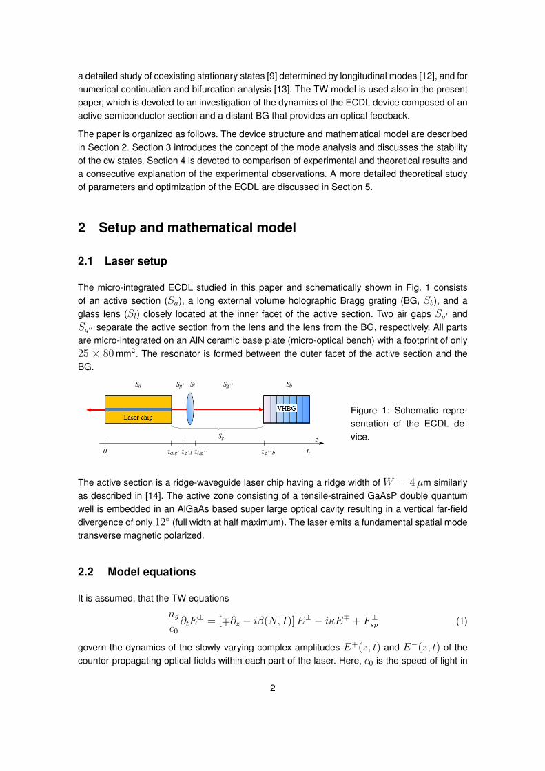
The micro-integrated ECDL studied in this paper and schematically shown in Fig. 1 consistsof an active section (Sa), a long external volume holographic Bragg grating (BG, Sb), and aglass lens (Sl) closely located at the inner facet of the active section. Two air gaps Sg′ andSg′′ separate the active section from the lens and the lens from the BG, respectively. All partsare micro-integrated on an AlN ceramic base plate (micro-optical bench) with a footprint of only25 × 80 mm2. The resonator is formed between the outer facet of the active section and theBG.

0 a,g’ g’,l l,g’’ g’’,b L

zg

a g’ l g’’ bS

z z z z

S

S SSS

Figure 1: Schematic repre-sentation of the ECDL de-vice.

The active section is a ridge-waveguide laser chip having a ridge width of W = 4µm similarlyas described in [14]. The active zone consisting of a tensile-strained GaAsP double quantumwell is embedded in an AlGaAs based super large optical cavity resulting in a vertical far-fielddivergence of only 12 (full width at half maximum). The laser emits a fundamental spatial modetransverse magnetic polarized.

2.2 Model equations

It is assumed, that the TW equations

ngc0

∂tE± = [∓∂z − iβ(N, I)]E± − iκE∓ + F±sp (1)

govern the dynamics of the slowly varying complex amplitudes E+(z, t) and E−(z, t) of thecounter-propagating optical fields within each part of the laser. Here, c0 is the speed of light in

2

vacuum, F±sp is the stochastic spontaneous emission term in the active section Sa, ng is thegroup index (different within different parts of the device), and κ is the field coupling coefficient(non-vanishing only in the Bragg grating Sb).

At the output ports of the ECDL (z = 0 and z = L) as well as at the interfaces z = zk,j of theadjacent parts Sk and Sj of the device where k, j ∈ a, g′, l, g′′, b (see Fig. 1), the complexoptical fields are related by the following reflection/transmission conditions [12]:

E+(0, t) = −r∗0E−(0, t), E−(L, t) = rLE+(L, t),

E+(z+k,j, t) = −r∗k,jE−(z+

k,j, t) + tk,jE+(z−k,j, t),

E−(z−k,j, t) = rk,jE+(z−k,j, t) + tk,jE

−(z+k,j, t).

(2)

Here z−k,j and z+k,j denote the left and the right sides of the section interface, whereas rk,j are

the complex field amplitude reflectivity coefficients (|rk,j| ≤ 1) and tk,j =√

1− |rk,j|2 are thetransmission coefficients.

The relative propagation factor β is given by

β = δ − iα2− iD

2+ δT (I) + i

(1 + iαH)Γg′ (N −Ntr)

2. (3)

Outside the active section Sa the only non-vanishing terms in the expression (3) can be theinternal loss constant α and the field phase tuning δ. In the absence of the field reflections atthe edges of the lens (rg′,l = rl,g′′ = 0) as it is considered in this paper, the three sequentparts Sg′ , Sl, and Sg′′ of the ECDL can be treated as a single gap section Sg with the averagedgroup index 〈ng〉g, phase tuning 〈δ〉g, and loss 〈α〉g. Here,

〈ζ〉k =1

|Sk|

∫Sk

ζ(z)dz

denotes a spatial average of a function ζ over any ECDL section Sk, whereas |Sk| is the lengthof Sk. The TW equations (1) in Sg can be easily resolved implying

E+(z−g′′,b, t) =√ηeiϕ/2E+(z+

a,g′ , t− τg),E−(z+

a,g′ , t) =√ηeiϕ/2E−(z−g′′,b, t− τg),

where

η = e−〈α〉g |Sg |,ϕ

2= −〈δ〉g|Sg|, and τk =

〈ng〉k|Sk|c0

are the intensity attenuation, the phase shift of the forward or backward field during its propaga-tion along Sg, and the field propagation time along each ECDL part Sk, respectively.

Within the active section Sa, the remaining terms of the propagation factor β are nontrivial. Theoperator D together with the induced polarization functions P±(z, t) are used to model thedispersion of material gain by a Lorentzian approximation [10]:

DE± = g(E±− P±), ∂tP± = γ(E±− P±) + iωP±, (4)

3

where g, ω, 2γ are the amplitude, the relative central frequency, and the full width at the halfmaximum of this Lorentzian. The function δT (I) represents the dependence of the refractiveindex on the heating induced by the injected current I , e.g. [15]:

δT (I) = cT I. (5)

Finally, β depends also on the carrier density dependent gain and index change functions de-termined by the confinement factor Γ, differential gain g′, linewidth enhancement (Henry) factorαH , and transparency carrier densityNtr. Due to the fact, that in the ECDL under study the over-all variation of the carrier density N is small, a linear dependence on N has been assumed.

The longitudinal distribution of the local photon density |E(z, t)|2 = |E+|2 + |E−|2 within theactive section Sa of the ECDL deviates only slightly from its spatial average, 〈|E|2〉a. For thisreason we neglect the spatial hole-burning of carriers and define the evolution of the spatially-uniform carrier density N(t) in the active section Sa by the following rate equation:

∂tN =I

qσ|Sa|−(AN +BN2 + CN3

)− c0

ng<∑ν=±

〈Eν∗ [Γg′(N−Ntr)−D]Eν〉a, (6)

where A, B, C are carrier recombination parameters, I , σ, and q denote the injected current,the cross-section area of the active zone, and the electron charge. The emitted field power atthe facet z = 0 is given by

Po(t) = (1− |r0|2)σc0

ng

hc0

λ0

|E−(0, t)|2, (7)

where h is the Planck constant, λ0 is the central wavelength, and 1− |r0|2 is the field intensitytransmission through the facet.

2.3 Typical parameters

The ECDL operates at λ0 = 0.78µm. As it was mentioned above, the amplitude reflectivitiesrg′,l = rl,g′′ = 0. Other reflectivities are ra,g′ = 0.01, rg′′,b = rL = 0, and r0 =

√0.3. The

lengths of sections are |Sa| = 1 mm, |Sb| = 6 mm, and |Sg| = 30 mm (where |Sg′|, |Sl|, and|Sg′′ | are 1, 2, and 27 mm, respectively).

The numerical scheme used for integration of the TW equations (1) implies the condition ht =(ng/c0)hz,k [12] on the temporal domain discretization step ht and the spatial steps hz,kwithin each ECDL section Sk. All sections should consist of an integer number of steps hz,i.e. |Sk|ng/(c0ht) should be integer for all k. Since the group indices ng in individual sections,in general, are different, one can fulfil this condition simultaneously for all Sk either by a carefulchoice of the section lengths, or by a corresponding adaptation of ng. The group indices ng inSa, Sb, Sl, and Sg′,g′′ used in this paper are 4.1, 1.48625, 1.6005, and 1, respectively (such that〈ng〉g in Sg is, approximately, 1.04).

The numerical grid of the considered problem is determined by the temporal steps ht ≈ 68.33fs, whereas the longitudinal domain [0, L] of the whole ECDL is discretized by 2157 spatialsteps, with 200 of them discretizing the section Sa.

4

Without loss of generality, one can assume a vanishing phase tuning δ in all sections but Sa,where δ ≈ −0.8 cm−1, which allows to obtain a good agreement between the consideredsimple linear and more accurate nonlinear models for gain and index change functions. Theabsorption coefficients α in Sa and Sb are 2 cm−1 and 0 cm−1, respectively. The attenuationη = 0.8 within Sg implies 〈α〉g ≈ 7.438 m−1.

0

0.5

1

Rm

ax

0 1 2 3 4 5

κ |Sb|

6

8

10

12

ωS

Bτ

b

-10 -5 0 5 10

scaled relative frequency [ ω τb ]

0

0.2

0.4

0.6

0.8

1

pow

er re

flec

tivit

y

κ|Sb|=1

κ|Sb|=2

κ|Sb|=3

κ|Sb|=4

(a) (b)

(c)

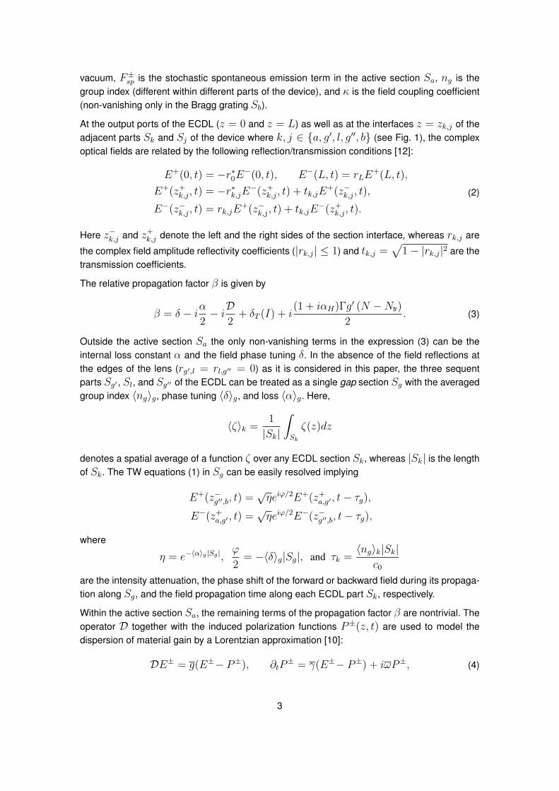
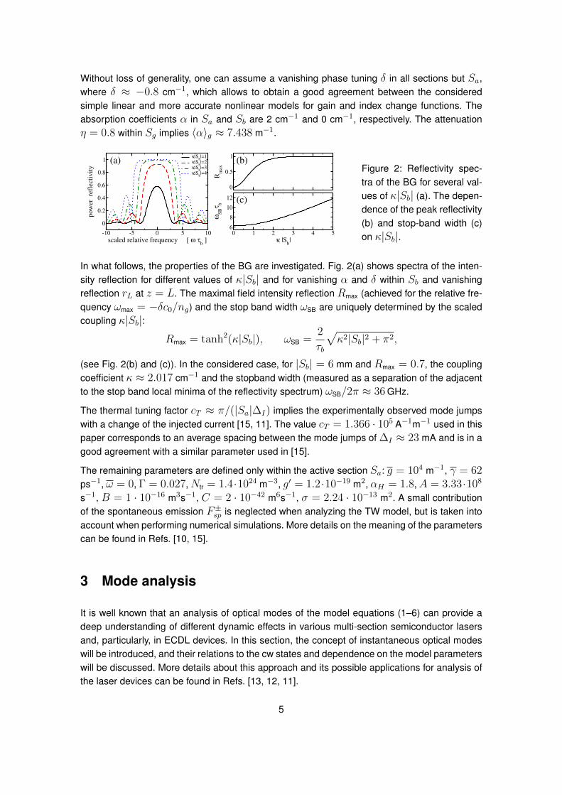
Figure 2: Reflectivity spec-tra of the BG for several val-ues of κ|Sb| (a). The depen-dence of the peak reflectivity(b) and stop-band width (c)on κ|Sb|.

In what follows, the properties of the BG are investigated. Fig. 2(a) shows spectra of the inten-sity reflection for different values of κ|Sb| and for vanishing α and δ within Sb and vanishingreflection rL at z = L. The maximal field intensity reflection Rmax (achieved for the relative fre-quency ωmax = −δc0/ng) and the stop band width ωSB are uniquely determined by the scaledcoupling κ|Sb|:

Rmax = tanh2(κ|Sb|), ωSB =2

τb

√κ2|Sb|2 + π2,

(see Fig. 2(b) and (c)). In the considered case, for |Sb| = 6 mm and Rmax = 0.7, the couplingcoefficient κ ≈ 2.017 cm−1 and the stopband width (measured as a separation of the adjacentto the stop band local minima of the reflectivity spectrum) ωSB/2π ≈ 36 GHz.

The thermal tuning factor cT ≈ π/(|Sa|∆I) implies the experimentally observed mode jumpswith a change of the injected current [15, 11]. The value cT = 1.366 · 105 A−1m−1 used in thispaper corresponds to an average spacing between the mode jumps of ∆I ≈ 23 mA and is in agood agreement with a similar parameter used in [15].

The remaining parameters are defined only within the active section Sa: g = 104 m−1, γ = 62ps−1, ω = 0, Γ = 0.027,Ntr = 1.4·1024 m−3, g′ = 1.2·10−19 m2, αH = 1.8,A = 3.33·108

s−1, B = 1 · 10−16 m3s−1, C = 2 · 10−42 m6s−1, σ = 2.24 · 10−13 m2. A small contributionof the spontaneous emission F±sp is neglected when analyzing the TW model, but is taken intoaccount when performing numerical simulations. More details on the meaning of the parameterscan be found in Refs. [10, 15].

3 Mode analysis

It is well known that an analysis of optical modes of the model equations (1–6) can provide adeep understanding of different dynamic effects in various multi-section semiconductor lasersand, particularly, in ECDL devices. In this section, the concept of instantaneous optical modeswill be introduced, and their relations to the cw states and dependence on the model parameterswill be discussed. More details about this approach and its possible applications for analysis ofthe laser devices can be found in Refs. [13, 12, 11].

5

3.1 Instantaneous optical modes

Instantaneous optical modes are sets of complex-valued objects (Θ(z),Ω), which satisfy thespectral problem generated by the substitution of the expression

E(z, t) = Θ(z)eiΩt

into the field equations (1), (2), and (4). Both Θ(z) and Ω depend on the instantaneous valueof carrier density N(t) = N . The real and imaginary parts of the complex eigenvalue Ω of thespectral problem represent an optical frequency and damping of the mode, respectively. Thevector-eigenfunction Θ(z) gives us the spatial profile of the longitudinal mode [12].

For the simple case, when α0, δ0 in Sb, κ in Sa, and rg′,l, rl,g′′ , rg′,b, rL are vanishing, thesubstitution of the expression for the field function into (1) and the resolution of the resultingsystem of ODEs implies the complex equation

G(N ,Ω)R(Ω)e−2iΩτg = η−1e−iϕ, (8)

where the active-section and BG response functions G andR, respectively, are given by

G(N ,Ω) =Θ+(z+

a,g′)

Θ−(z+a,g′)

= −(r∗0 + r∗a,g′e

i2Da(N,Ω))(

r∗0ra,g′ + ei2Da(N,Ω)) ,

Da(N ,Ω) = Ωτa +

[(i+αH)Γg′

(N−Ntr

)2

+g

2

(Ω− ω)

γ + i (Ω− ω)− iα

2+ δ + cT I

]|Sa|,

R(Ω) =Θ−(z−g′′,b)

Θ+(z−g′′,b)=

−iκ|Sb|iΩτb +Db(Ω) cotDb(Ω)

,

Db(Ω) =√

Ω2τ 2b − κ2|Sb|2.

The complex nonlinear characteristic equation (8) has an infinite number of complex roots Ω,most of which are well damped and play no role in the dynamics of the laser device (for moredetails see Ref. [12]).

0

0.2

0.4

0.6

refl

ecti

vit

y

-60 -40 -20 0 20 40 60

relative frequency Re Ω / 2π [GHz]

0

2

4

6

8

10

12

dam

pin

g

[1

/ns]

(a)

(b)

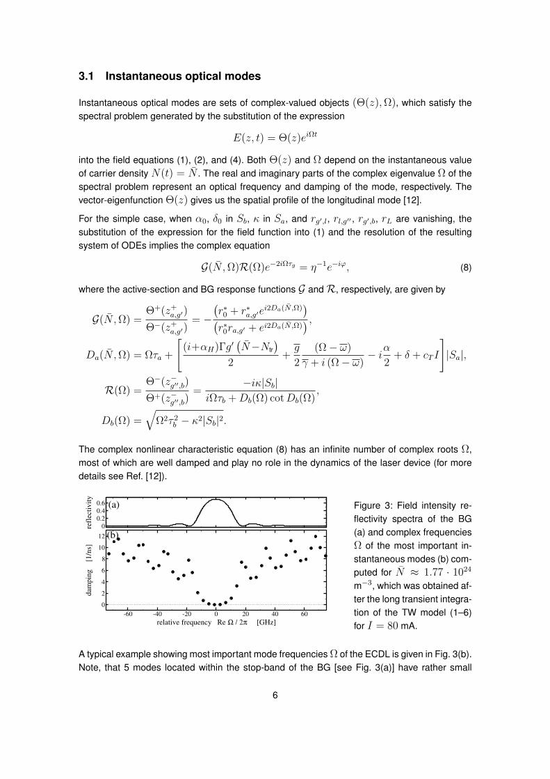
Figure 3: Field intensity re-flectivity spectra of the BG(a) and complex frequenciesΩ of the most important in-stantaneous modes (b) com-puted for N ≈ 1.77 · 1024

m−3, which was obtained af-ter the long transient integra-tion of the TW model (1–6)for I = 80 mA.

A typical example showing most important mode frequencies Ω of the ECDL is given in Fig. 3(b).Note, that 5 modes located within the stop-band of the BG [see Fig. 3(a)] have rather small

6

damping, which does not exceed 1 ns−1. Thus, a strong influence of the side modes still canbe expected, even though the ECDL operates at a cw state determined by one of these modes.Some possibilities for improving the mode selection will be discussed later in Section 5.

3.2 Stationary states

All stationary (continuous wave) states of the TW model (1–6) can be written as(E(z, t)N(t)

)=

(Θ(z)eiωt

N

), (9)

where (Θ(z), ω) is an instantaneous optical mode computed at the mode threshold carrierdensity N , which provides the real-valued mode frequency ω, i.e., determines the mode withno damping or amplification. Thus, in order to find all possible cw states we need to find all realpairs (N , ω), which satisfy the characteristic equation (8). The method of definition of the cwstates is similar to that frequently used in the analysis of the Lang-Kobayashi (LK) model forlasers with delayed optical feedback [6], where the corresponding cw states are well known asexternal cavity modes.

Once N and ω are known, one can easily reconstruct the spatial distribution of the optical fields(function Θ(z)), which is a solution of the ODE system obtained after substitution of the fieldfunction from (9) into the TW problem (1), (2). The intensity P of the cw state emitted from theECDL at the facet z = 0 can be found from the carrier rate equation (6):

Po =(1− |r0|2)σ hc0

λ0

(I

qσ|Sa| − AN −BN2 − CN3

)[Γg′(N−Ntr)− g(ω−ω)2

γ2+(ω−ω)2

](e−=Da+|r0|2)(e=Da−1)

=Da

.

It is clear, that it only makes sense to discuss the cw states with positive intensity, i.e., the stateswith the threshold N satisfying the inequality I > qσ|Sa|

(AN +BN2 + CN3

).

The complex equation (8) for real frequency Ω = ω and threshold density N is equivalent tothe system of two real equations

η =∣∣G(N , ω)R(ω)

∣∣−1,

ϕ = 2ωτg − arg[G(N , ω)R(ω)

]mod 2π,

(10)

representing η and ϕ as the functions of two variables, N and ω. Thus, each pair (N , ω)uniquely defines the values of η and ϕ, and, therefore, determine a cw state of the ECDLdevice with this pair of parameters. Those (N , ω) giving η = 0.8 and ϕ = 0 (ECDL parametersdefined in Subsection 2.3) are the roots of Eq. (10) and define the cw states of the consideredECDL.

A following geometric interpretation of Eqs. (10) suggests a relatively easy method for locationof the roots (N , ω) for any fixed parameters η and ϕ. Namely, each of the equations determinessome curves in the (N , ω) plane: see solid and dashed curves in Fig. 4. The intersections ofdifferent curves are the roots of Eq. (10) (bullets in the same figure).

7

-40 -20 0 20 40

relative frequency ω / 2π [GHz]

1.8

2

2.2

thre

sho

ld d

ensi

ty

N

[

10

24/m

3 ]

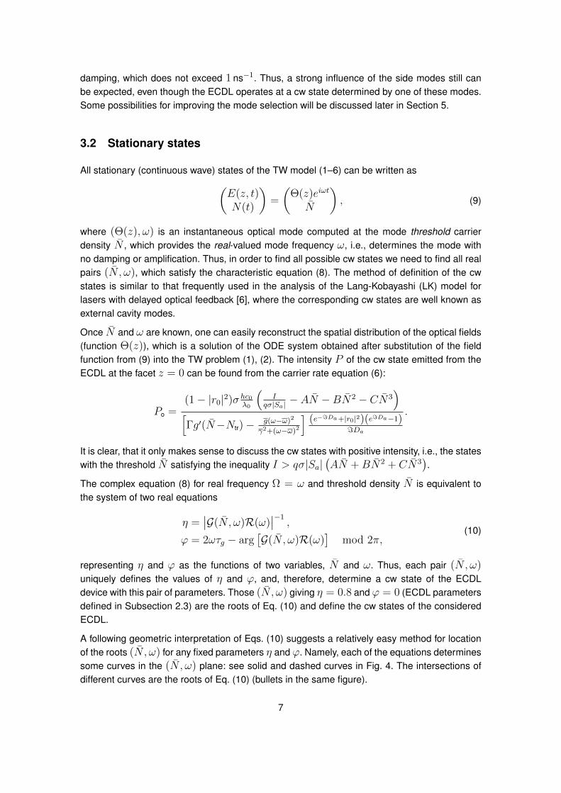
Figure 4: Representation ofcw states in mode frequencyω - mode threshold N do-main. Solid: cw states forfixed η = 0.8. Dashed: cwstates for fixed ϕ = 0. Bul-lets: cw states for fixed ϕand η. All other parametersas in Subsection 2.3.

The solid curves in Fig. 4, which are the contour lines of η(N , ω), represent the roots of theconsidered system for η = 0.8 and arbitrary ϕ. The phase factor at each point of the curvecan be easily determined by the second equation of (10). Thus, these curves are illustrating thecontinuation of all possible cw states (denoted by multiple bullets for ϕ = 0 in Fig. 4) whentuning the phase parameter ϕ. Tuning of ϕ leads to the shift of these states along the curvesand the replacement of the next neighbor cw state on the curve with the periodicity ϕ = 2π.

Similarly, the dashed curves in Fig. 4 (the contour lines of ϕ(N , ω) for ϕ = 0) correspond tocw states obtained by continuation of η. Sudden endings of these lines at certain values of ωare related to the zeroes of the functionR(ω) where factor η turns to infinity.

It is noteworthy, that the solid curves in Fig. 4 give a similar representation of the cw states asellipses of external cavity modes in the LK model.

3.3 Multi-stability

The mode analysis and the location of the cw states discussed above do not provide any in-formation about stability of these cw states. In general, a detailed investigation of the stabilityof the states can be performed by means of numerical bifurcation analysis [13]. In this paper,however, the stability of each cw state is identified by its ability to attract trajectories duringnumerical integration of the model equations.

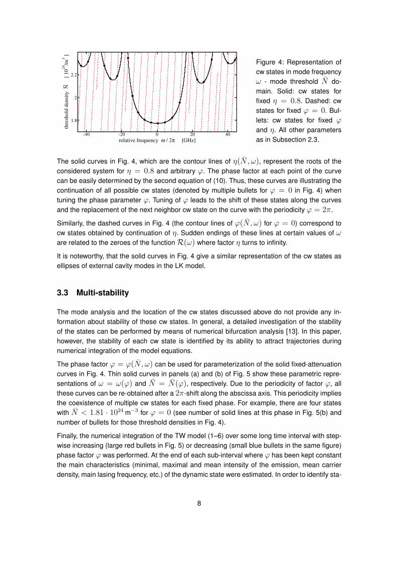
The phase factor ϕ = ϕ(N , ω) can be used for parameterization of the solid fixed-attenuationcurves in Fig. 4. Thin solid curves in panels (a) and (b) of Fig. 5 show these parametric repre-sentations of ω = ω(ϕ) and N = N(ϕ), respectively. Due to the periodicity of factor ϕ, allthese curves can be re-obtained after a 2π-shift along the abscissa axis. This periodicity impliesthe coexistence of multiple cw states for each fixed phase. For example, there are four stateswith N < 1.81 · 1024 m−3 for ϕ = 0 (see number of solid lines at this phase in Fig. 5(b) andnumber of bullets for those threshold densities in Fig. 4).

Finally, the numerical integration of the TW model (1–6) over some long time interval with step-wise increasing (large red bullets in Fig. 5) or decreasing (small blue bullets in the same figure)phase factor ϕ was performed. At the end of each sub-interval where ϕ has been kept constantthe main characteristics (minimal, maximal and mean intensity of the emission, mean carrierdensity, main lasing frequency, etc.) of the dynamic state were estimated. In order to identify sta-

8

-10

-5

0

5fr

equen

cy

ω /

2π

[G

Hz]

-1 -0.5 0 0.5 1 1.5

phase factor ϕ / 2π

1.77

1.78

1.79

1.8

thre

shold

N

[

10

24/m

3 ]

(a)

(b)

s1

s2

s2

s3

s1

s3

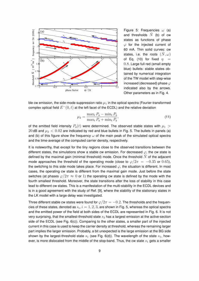
Figure 5: Frequencies ω (a)and thresholds N (b) of cwstates as functions of phaseϕ for the injected current of60 mA. Thin solid curves: cwstates, i.e. the roots (N , ω)of Eq. (10) for fixed η =0.8. Large full red (small emptyblue) bullets: stable states ob-tained by numerical integrationof the TW model with step-wiseincreased (decreased) phaseϕindicated also by the arrows.Other parameters as in Fig. 4.

ble cw emission, the side-mode suppression ratio µ1 in the optical spectra (Fourier-transformedcomplex optical field E−(0, t) at the left facet of the ECDL) and the relative deviation

µ2 =maxt Po −mint Po

maxt Po + mint Po, (11)

of the emitted field intensity Po(t) were determined. The observed stable states with µ1 >20 dB and µ2 < 0.02 are indicated by red and blue bullets in Fig. 5. The bullets in panels (a)and (b) of this figure show the frequency ω of the main peak of the simulated optical spectraand the time-average of the computed carrier density, respectively.

It is noteworthy, that except for the tiny regions close to the observed transitions between thedifferent states, the simulations show a stable cw emission. For decreased ϕ, the cw state isdefined by the maximal gain (minimal threshold) mode. Once the threshold N of the adjacentmode approaches the threshold of the operating mode (close to ϕ/2π = −0.35 or 0.65),the switching to this side mode takes place. For increased ϕ, the situation is different. In mostcases, the operating cw state is different from the maximal gain mode. Just before the stateswitches (at phases ϕ/2π ≈ 0 or 1) the operating cw state is defined by the mode with thefourth smallest threshold. Moreover, the state transitions after the loss of stability in this caselead to different cw states. This is a manifestation of the multi-stability in the ECDL devices andis in a good agreement with the study of Ref. [9], where the stability of the stationary states inthe LK model with a large delay was investigated.

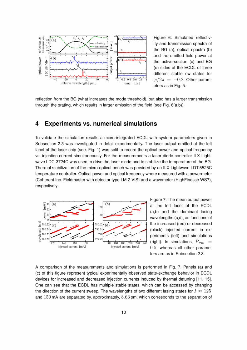
Three different stable cw states were found for ϕ/2π = −0.2. The thresholds and the frequen-cies of these states, denoted as si, i = 1, 2, 3, are shown in Fig. 5, whereas the optical spectraand the emitted power of the field at both sides of the ECDL are represented in Fig. 6. It is notvery surprising, that the smallest-threshold state s3 has a largest emission at the active-sectionside of the ECDL (see Fig. 6(c)). Comparing to the other states, a smaller part of the injectedcurrent in this case is used to keep the carrier density at threshold, whereas the remaining largerpart implies the larger emission. Probably, a bit unexpected is the large emission at the BG sideshown by the largest-threshold state s1 (see Fig. 6(d)). The wavelength of the state s1, how-ever, is more dislocated from the middle of the stop-band. Thus, the cw state s1 gets a smaller

9

-40 -20 0 20 40 60

relative vawelength [ pm ]

opti

cal

pow

er

[ 20 d

B /

div

. ]

20

21

22

0 0.2 0.4 0.6 0.8 1

time [ns]

6

7

8

outp

ut

pow

er [

mW

]

0

0.2

0.4

0.6

0.81

refl

ecti

on &

tran

smis

sion

reflectivity

transmission

(d)s

3

s2

(b)

(c)

s1

s3

s2

s1

s1

s2

s3

(a)s

3 s2

s1

Figure 6: Simulated reflectiv-ity and transmission spectra ofthe BG (a), optical spectra (b)and the emitted field power atthe active-section (c) and BG(d) sides of the ECDL of threedifferent stable cw states forϕ/2π = −0.2. Other param-eters as in Fig. 5.

reflection from the BG (what increases the mode threshold), but also has a larger transmissionthrough the grating, which results in larger emission of the field (see Fig. 6(a,b)).

4 Experiments vs. numerical simulations

To validate the simulation results a micro-integrated ECDL with system parameters given inSubsection 2.3 was investigated in detail experimentally. The laser output emitted at the leftfacet of the laser chip (see. Fig. 1) was split to record the optical power and optical frequencyvs. injection current simultaneously. For the measurements a laser diode controller ILX Light-wave LDC-3724C was used to drive the laser diode and to stabilize the temperature of the BG.Thermal stabilization of the micro-optical bench was provided by an ILX Lightwave LDT-5525Ctemperature controller. Optical power and optical frequency where measured with a powermeter(Coherent Inc. Fieldmaster with detector type LM-2 VIS) and a wavemeter (HighFinesse WS7),respectively.

120 140 160 180

injected current [mA]

780.22

780.23

780.24

780.25

wav

elen

gth

[nm

]

80

120

140 160 180 200 220 240

injected current [mA]

779.99

780

780.01

780.02

15

20

25

30

pow

er [m

W]

(d)

(b)

(c)

(a)Figure 7: The mean output powerat the left facet of the ECDL(a,b) and the dominant lasingwavelengths (c,d), as functions ofthe increased (red) or decreased(black) injected current in ex-periments (left) and simulations(right). In simulations, Rmax =0.5, whereas all other parame-ters are as in Subsection 2.3.

A comparison of the measurements and simulations is performed in Fig. 7. Panels (a) and(c) of this figure represent typical experimentally observed state-exchange behavior in ECDLdevices for increased and decreased injection currents induced by thermal detuning [11, 15].One can see that the ECDL has multiple stable states, which can be accessed by changingthe direction of the current sweep. The wavelengths of two different lasing states for I ≈ 125and 150 mA are separated by, approximately, 8.63 pm, which corresponds to the separation of

10

the neighboring optical modes within the stop-band of the BG. The two times larger wavelengthseparation for I ≈ 140 and between 155 and 186 mA indicates a possible coexistence of thethird stable state, which could be accessed by a change of the direction of the current sweepjust after each jump of the states.

The similar simulated state-jumping behavior is represented in panels (b) and (d) of the same fig-ure. In order to obtain the good agreement between measurement and simulation, the maximumreflectivity of the BG has to been changed from the intended value Rmax = 0.7 to Rmax = 0.5by a corresponding adaptation of the coupling coefficient κ. The reasons for this adjustmentcould be, for example, the divergence of the beam within the BG and an imperfect alignment ofthe BG with respect to the optical axis of the ECDL.

It is noteworthy, that the states observed during the down-sweeping of the injection current havelarger intensities, as compared to the up-sweeping case. The wavelengths of these states arelocated close to the center of the BG stop-band, which in our simulations is at 780 nm. Smalldifferences of the emitted field intensities before and after mode jumps in this case can be wellexplained by the similar emission power of the states s3 and s2, see Fig. 6(c) and discussionof Subsection 3.3. On contrary, the state jumps for up-swept injection correspond to detuninginduced transitions between states s1 and s2 or s1 and s3 (see Figs. 5 and 6), what explainsthe large step-like increase of the emission intensity at each state transition.

5 Discussion

As it was mentioned above, the dynamics of the ECDL device is determined by several modesin many cases. In order to achieve a controllable stable lasing on a single mode, one needs toimprove the mode selection, which, particularly, can be achieved by a reduction of the numberof the main modes almost equally supported by the BG.

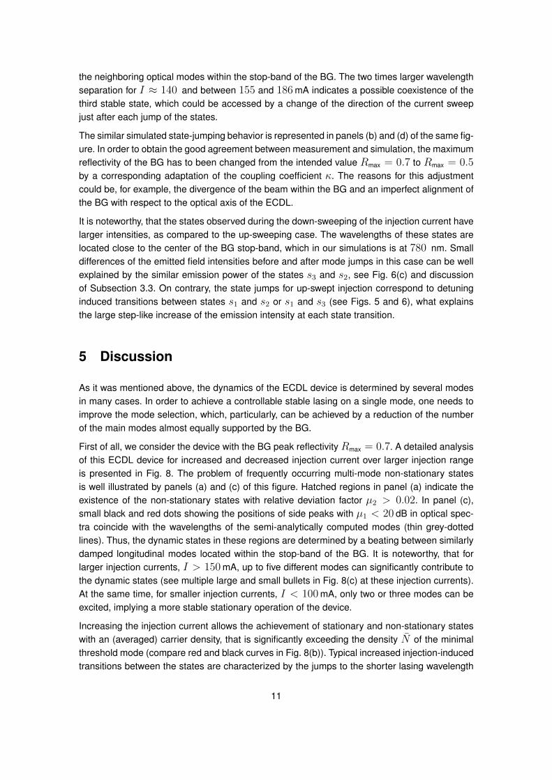
First of all, we consider the device with the BG peak reflectivity Rmax = 0.7. A detailed analysisof this ECDL device for increased and decreased injection current over larger injection rangeis presented in Fig. 8. The problem of frequently occurring multi-mode non-stationary statesis well illustrated by panels (a) and (c) of this figure. Hatched regions in panel (a) indicate theexistence of the non-stationary states with relative deviation factor µ2 > 0.02. In panel (c),small black and red dots showing the positions of side peaks with µ1 < 20 dB in optical spec-tra coincide with the wavelengths of the semi-analytically computed modes (thin grey-dottedlines). Thus, the dynamic states in these regions are determined by a beating between similarlydamped longitudinal modes located within the stop-band of the BG. It is noteworthy, that forlarger injection currents, I > 150 mA, up to five different modes can significantly contribute tothe dynamic states (see multiple large and small bullets in Fig. 8(c) at these injection currents).At the same time, for smaller injection currents, I < 100 mA, only two or three modes can beexcited, implying a more stable stationary operation of the device.

Increasing the injection current allows the achievement of stationary and non-stationary stateswith an (averaged) carrier density, that is significantly exceeding the density N of the minimalthreshold mode (compare red and black curves in Fig. 8(b)). Typical increased injection-inducedtransitions between the states are characterized by the jumps to the shorter lasing wavelength

11

50 100 150 200 250

injected current [mA]

-10

0

10

20

rela

tiv

e w

avel

eng

th [

pm

]

1.75

1.8

1.85

den

sity

[1

024/m

3]

0

50

100

150

200

mea

n p

ow

er

[mW

]

(a)

(b)

(c)

left side

right side

Figure 8: Mean output power atthe left (solid) and right (dashed)sides of the ECDL (a), mean car-rier density in Sa (b), and thelasing wavelengths (c) as func-tions of the increased (red) or de-creased (black) injected current.All parameters are as in Subsec-tion 2.3. Horizontally and verti-cally hatched areas in (a) indi-cate non-stationary regimes forincreased or decreased currents,respectively. Big bullets and smalldots in (c) represent the main op-tical mode and the side modessuppressed by less than 20 dB,respectively. Thin dashed greylines in the same panel show po-sitions of all longitudinal modes.

located closer to the central wavelength of the BG [red bullets in panel (c)], sudden reduction ofthe mean carrier density [panel (b)] and increase (decrease) of the (mean) emission intensityat the left (right) output port of the ECDL [panel (a)]. The lasing wavelength and emission inten-sities before and after the transitions are similar to those of the states s1 and s2 discussed inSubsection 3.3 and shown in Fig. 6. A corresponding transition from s1 to s2 was also shownin Fig. 5 at the phase ϕ ≈ 0. The jumps of the carrier density and emission intensities fordecreased injection current are less pronounced, since the dominant mode wavelengths arecloser to the middle of the stop-band and their thresholds are rather similar.

50 100 150 200 250

injected current [mA]

-10

0

10

20

rela

tiv

e λ

[p

m]

0

50

100

150

200

mea

n p

ow

er

[mW

]

50 100 150 200 250

injected current [mA]

(a)

(c)

(b)

(d)

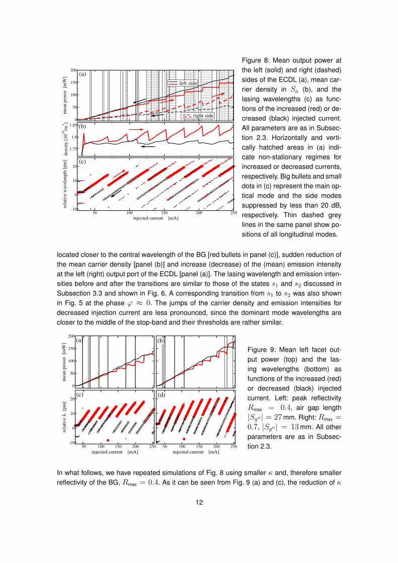
Figure 9: Mean left facet out-put power (top) and the las-ing wavelengths (bottom) asfunctions of the increased (red)or decreased (black) injectedcurrent. Left: peak reflectivityRmax = 0.4, air gap length|Sg′′ | = 27 mm. Right: Rmax =0.7, |Sg′′ | = 13 mm. All otherparameters are as in Subsec-tion 2.3.

In what follows, we have repeated simulations of Fig. 8 using smaller κ and, therefore smallerreflectivity of the BG, Rmax = 0.4. As it can be seen from Fig. 9 (a) and (c), the reduction of κ

12

implies a reduction of the emission intensity at the left side of the ECDL, and, which is ratherimportant, stabilizes the laser operation between the mode transitions. The gratings with largeκ|Sb| ≥ 2 have a flat stop-band [see Fig. 2(a)], which can equally support multiple modes(once they are located within such a stop-band). Thus, even though the choice of a smallerκ|Sb| ≈ 0.75 [see Fig. 2(b)] reduces the overall reflectivity of the grating and implies an un-wanted increase of the lasing threshold as well as decrease of the emission intensity, it helps toimprove the side mode suppression.

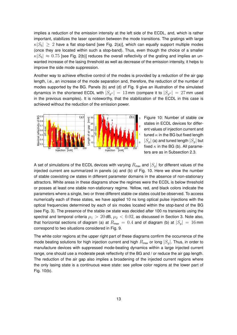
Another way to achieve effective control of the modes is provided by a reduction of the air gaplength, i.e., an increase of the mode separation and, therefore, the reduction of the number ofmodes supported by the BG. Panels (b) and (d) of Fig. 9 give an illustration of the simulateddynamics in the shortened ECDL with |Sg′′ | = 13 mm (compare it to |Sg′′ | = 27 mm usedin the previous examples). It is noteworthy, that the stabilization of the ECDL in this case isachieved without the reduction of the emission power.

50 100 150 200 250Injection [mA]

0.3

0.4

0.5

0.6

0.7

0.8

0.9

Ma

xim

al re

fle

ctivity o

f B

G

0

1

2

3"LR2175LP_3d_data.dat" u 2:1:($3*(1-$6))

50 100 150 200 250Injection [mA]

10

15

20

25

30

Le

ng

th o

f a

ir g

ap

[

mm

]

0

1

2

3(a) (b)

off

−st

ate

off

−st

ate

Figure 10: Number of stable cwstates in ECDL devices for differ-ent values of injection current andtuned κ in the BG but fixed length|Sg| (a) and tuned length |Sg| butfixed κ in the BG (b). All parame-ters are as in Subsection 2.3.

A set of simulations of the ECDL devices with varying Rmax and |Sg| for different values of theinjected current are summarized in panels (a) and (b) of Fig. 10. Here we show the numberof stable coexisting cw states in different parameter domains in the absence of non-stationaryattractors. White areas in these diagrams show the regimes were the ECDL is below thresholdor posses at least one stable non-stationary regime. Yellow, red, and black colors indicate theparameters where a single, two or three different stable cw states could be observed. To accessnumerically each of these states, we have applied 10 ns long optical pulse injections with theoptical frequencies determined by each of six modes located within the stop-band of the BG(see Fig. 3). The presence of the stable cw state was decided after 100 ns transients using thespectral and temporal criteria µ1 > 20 dB, µ2 < 0.02, as discussed in Section 3. Note also,that horizontal sections of diagram (a) at Rmax = 0.4 and of diagram (b) at |Sg| = 16 mmcorrespond to two situations considered in Fig. 9.

The white color regions at the upper right part of these diagrams confirm the occurrence of themode beating solutions for high injection current and high Rmax or long |Sg|. Thus, in order tomanufacture devices with suppressed mode-beating dynamics within a large injected currentrange, one should use a moderate peak reflectivity of the BG and / or reduce the air gap length.The reduction of the air gap also implies a broadening of the injected current regions wherethe only lasing state is a continuous wave state: see yellow color regions at the lower part ofFig. 10(b).

13

Acknowledgments

The authors would like to acknowledge the support of the German “Bundesministerium für Bil-dung und Forschung“ FKZ 01DK13020A (project MANUMIEL). VZT acknowledges the supportof the CIM-Returning Experts Programme and the project STCU 5937/14.820.18.02.012.

References

[1] D. N. Aguilera et al., “STE-QUEST-test of the universality of free fall using cold atom inter-ferometry,” Class. Quantum Grav., vol. 31, p. 115010, 2014.

[2] B. J. Bloom, T. L. Nicholson, J. R. Williams, S. L. Campbell, M. Bishof, X. Zhang, W. Zhang,S. L. Bromley, and J. Ye, “An optical lattice clock with accuracy and stability at the 1018

level,” Nature, vol. 506, pp. 71–75, 2014.

[3] T. Sodnik, B. Furch, and H. Lutz, “Optical Intersatellite Communication,” IEEE J. Select.Top. Quant. Electron., vol. 16, pp. 1051–1057, 2010.

[4] E. Luvsandamdin, C. Kürbis, M. Schiemangk, A. Sahm, A. Wicht, A. Peters, G. Erbert,and G. Tränkle, “Micro-integrated extended cavity diode lasers for precision potassiumspectroscopy in space,” Opt. Express, vol. 22, pp. 7790–7798, 2014.

[5] B. Krauskopf and D.Lenstra, Eds., Fundamental issues of nonlinear laser dynamics. AIPConf. Proc., vol. 548, 2000.

[6] R. Lang, and K. Kobayashi, “External optical feedback effects on semiconductor injectionlaser properties,” IEEE J. Quantum Electron., vol. 16, pp. 347–355, 1980.

[7] D. Lenstra, G. Vemuri, and M. Yousefi, “Generalized optical feedback: Theory,” in Unlockingdynamical diversity: Optical feedback effects on semiconductor lasers, D.M. Kane and K.A.Shore, Eds. John Wiley Sons, West Sussex, 2005, pp. 55–80.

[8] V.Z. Tronciu, H.-J. Wünsche, M. Wolfrum, and M. Radziunas “Semiconductor laser underresonant feedback from a Fabry-Perot resonator: Stability of continuous-wave operation,”Phys. Rev. E, vol. 73, 046205, 2006.

[9] S. Yanchuk and M. Wolfrum, “A multiple timescale approach to the stability of externalcavity modes in the Lang-Kobayashi system using the limit of large delay,” SIAM J. Appl.Dyn. Syst., vol. 9, pp. 519–535, 2010.

[10] U. Bandelow, M. Radziunas, J. Sieber, and M. Wolfrum, “Impact of gain dispersion on thespatio-temporal dynamics of multisection lasers,” IEEE J. Quantum Electron., vol. 37, pp.183–188, 2001.

[11] M. Radziunas, K.-H. Hasler, B. Sumpf, Tran Quoc Tien, and H. Wenzel, “Mode transitionsin DBR semiconductor lasers: Experiments, simulations and analysis,” J. Phys. B: At. Mol.Opt. Phys., vol. 44, p. 105401, 2011.

14

[12] M. Radziunas and H.-J. Wünsche, “Multisection lasers: longitudinal modes and their dy-namics,” in Optoelectronic devices – advanced simulation and analysis, J. Piprek, Ed. Sp-inger Verlag, 2005, pp. 121–150.

[13] M. Radziunas, “Numerical bifurcation analysis of traveling wave model of multisectionsemiconductor lasers,” Physica D, vol. 213, pp. 98–112, 2006.

[14] H. Wenzel, K. Häusler, G. Blume, J. Fricke, M. Spreemann, M. Zorn, and G. Erbert,“High-power 808 nm ridge-waveguide diode lasers with very small divergence, wavelength-stabilized by an external volume Bragg grating,” Optics Lett., vol. 34, pp. 1627–1629, 2009.

[15] M. Spreemann, M. Lichtner, M. Radziunas, U. Bandelow, and H. Wenzel, “Measurementand simulation of distributed-feedback tapered master-oscillators power-amplifiers,” IEEEJ. Quantum Electron., vol. 45, pp. 609–616, 2009.

15