Week 9

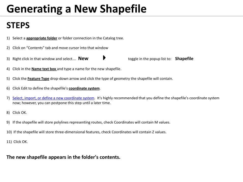
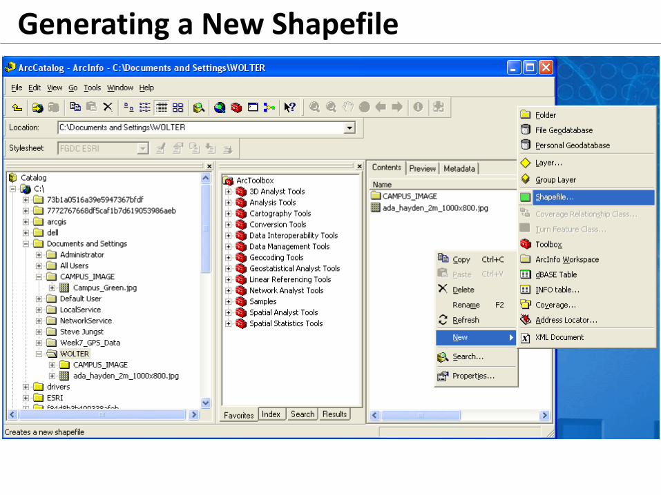
STEPS 1) Select a appropriate folder or folder connection in the Catalog tree.

2) Click on “Contents” tab and move cursor into that window

3) Right click in that window and select…. New toggle in the popup list to: Shapefile

4) Click in the Name text box and type a name for the new shapefile.

5) Click the Feature Type drop-down arrow and click the type of geometry the shapefile will contain.

6) Click Edit to define the shapefile's coordinate system.

7) Select, import, or define a new coordinate system. It's highly recommended that you define the shapefile's coordinate system now; however, you can postpone this step until a later time.

8) Click OK.

9) If the shapefile will store polylines representing routes, check Coordinates will contain M values.

10) If the shapefile will store three-dimensional features, check Coordinates will contain Z values.

11) Click OK.

The new shapefile appears in the folder's contents.

Generating a New Shapefile

Generating a New Shapefile

Generating a New Shapefile

Feature Types: • Point • Line ??? • Polygon

• Polyline • Multipoint • Multipatch

Generating a New Shapefile

Advanced Feature Types Polyline Polygon

POLYLINE Multiple line features stored as a single object • No polygon items or attributes • Unlike a single line feature, polylines can have

multiple thicknesses assigned etc. (e.g., county road, State HWY, US HWY)

• Used in Dynamic Segmentation

Endpoints Dynamic Seg.

Point and Line Events in one

Advanced Feature Types

MULTIPATCH

A 3D geometry used to represent the outer surface, or shell, of features that occupy a discrete area or volume in 3D space.

Here, planar 3D rings and triangles are used in combination to model a 3D shell.

Multipatches used to represent spheres, cubes, & iso-surfaces to form complex 3D shapes …..e.g., buildings

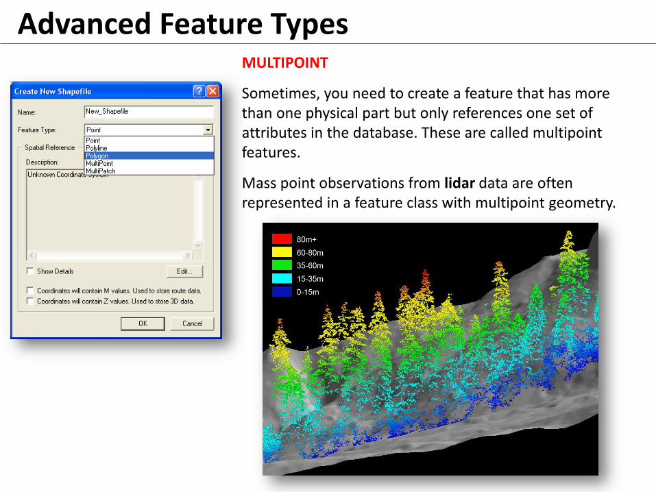
Advanced Feature Types MULTIPOINT

Sometimes, you need to create a feature that has more than one physical part but only references one set of attributes in the database. These are called multipoint features.

Mass point observations from lidar data are often represented in a feature class with multipoint geometry.

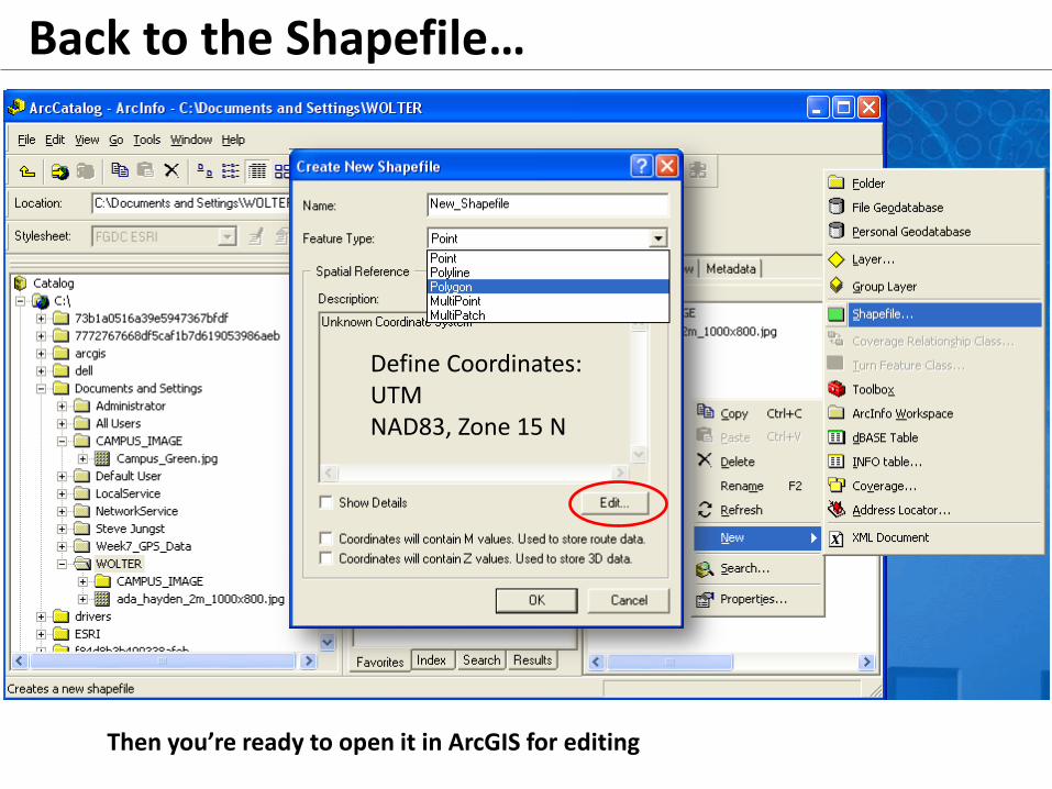
Back to the Shapefile…

Define Coordinates: UTM NAD83, Zone 15 N

Then you’re ready to open it in ArcGIS for editing

GIS Input Methods 1) Key board inputs

• x, y, attribute etc.

2) Land Survey & COGO • Section or ¼ section corners & use COGO to determine within-section parcel lines

3) Scanning & automatic line digitizing (R2V, VTRAC, etc)

4) “Heads-Up” digitizing directly form digital maps/photos/images • Manually digitize info right off the computer screen • Avoids some of the problems associated with paper map digitizing….

• Humidity affects paper map shape/size from day to day errors • Resulting digital line-work propagates these error • Difficult to reconcile…hard to know what is right • Scanning freezes the error in time, which remains constant day-to-day

5) Data input can become a major “bottleneck” of a GIS project

• Can cost 80% or more of project time • Labor intensive, tedious, error-prone • Constructing the GIS data can be so large that the project never finishes

6) Digitizing Bottom Line It is worth your while to do it as efficiently as possible

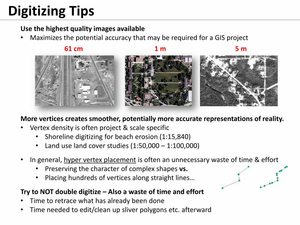
Digitizing Tips Use the highest quality images available • Maximizes the potential accuracy that may be required for a GIS project More vertices creates smoother, potentially more accurate representations of reality. • Vertex density is often project & scale specific

• Shoreline digitizing for beach erosion (1:15,840) • Land use land cover studies (1:50,000 – 1:100,000)

• In general, hyper vertex placement is often an unnecessary waste of time & effort • Preserving the character of complex shapes vs. • Placing hundreds of vertices along straight lines…

Try to NOT double digitize – Also a waste of time and effort • Time to retrace what has already been done • Time needed to edit/clean up sliver polygons etc. afterward

61 cm 1 m 5 m

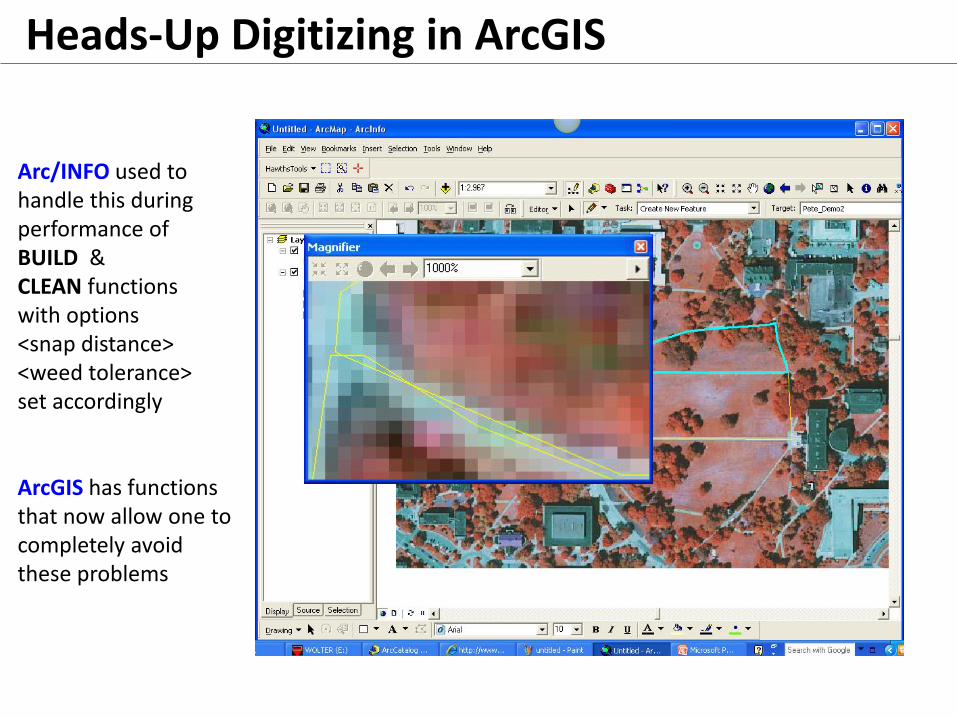
Heads-Up Digitizing in ArcGIS

Heads-Up Digitizing in ArcGIS

Arc/INFO used to handle this during performance of BUILD & CLEAN functions with options <snap distance> <weed tolerance> set accordingly ArcGIS has functions that now allow one to completely avoid these problems

Heads-Up Digitizing in ArcGIS

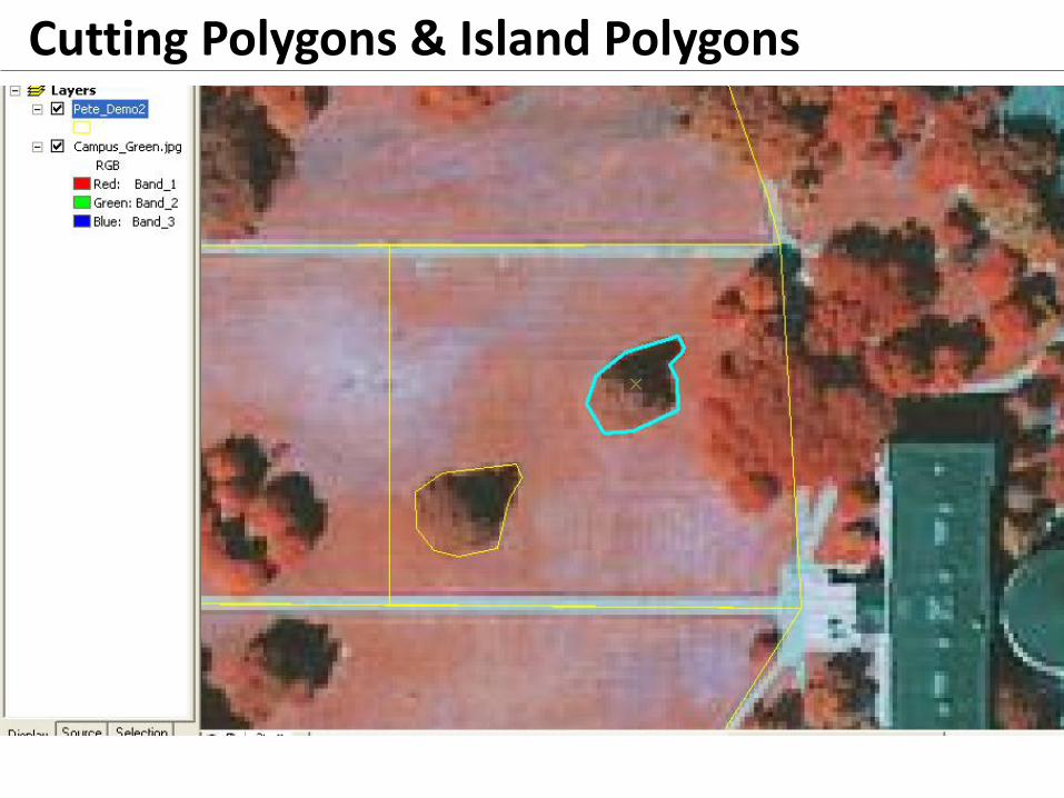
Cutting Polygons & Island Polygons

GPS Forecasting: Trimble’s “PLANNING”

ftp://ftp.trimble.com/pub/eph/ 1) Navigate to… 2) Open current Almanac 3) Copy it into “notepad” & save as “name.alm” 4) Open Planning, import ALM data, and set location or city

START HERE

Vector vs. Raster GIS Vector-based GIS – Discrete data - Discrete either in/on a polygon/line or not … no fuzziness in between - Stores graphic information as a series of points or nodes - All connecting lines are straight between nodes - Keeps all X, Y coordinates - Can accurately represent boundaries, but is computationally demanding

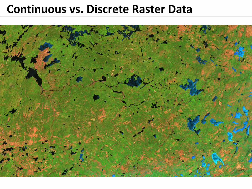
Raster-based GIS – Continuous data (Inherently fuzzy, seldom has clear boundaries) - Stores graphic information as a series of cells with a wide range of possible values…

- 8-bit integers (0-255 signed or not) Landsat & SPOT - 16-bit integers (0-63360 signed or not) AVHRR, MODIS, QuickBird - Single/Double/Quadruple precision floating point (32-bit/64-bit/128-bit)

- Ex: DEM data, LIDAR data, weather-climate data

- Rapid computation at expense of accuracy

- Data organized by ROW & COLUMN addressing

Developed Agricultural Forest Water Wetlands Barren Land

Discrete vs. Continuous Data

Continuous Data

Data in which each location on the surface is… • A relationship from a fixed point in space or • From a fixed emitting source or frame of reference

Examples: • Elevation – the fixed point being mean sea level (MSL) • Aspect – the fixed point being direction (N,S,E,W) • Satellite data - the fixed point being orientation w/ref to sun & terrain • Forested Lands or tree density – blends of species or bole arrangements

Discrete Data

• Object has a known or definable boundaries • Easy to define precisely where the object/feature begins and ends • Usually nouns: cover type, agricultural field, water bodies, lamp posts

Discrete Data Examples: Lake shore, buildings, roads, etc. Aspect – the fixed point being direction (N,S,E,W) Forested Lands or tree density – blends of species or arrangements

Continuous vs. Discrete Raster Data

Continuous vs. Discrete Raster Data

Continuous vs. Discrete Raster Data

Continuous vs. Discrete Raster Data

Continuous vs. Discrete Raster Data

Continuous vs. Discrete Raster Data

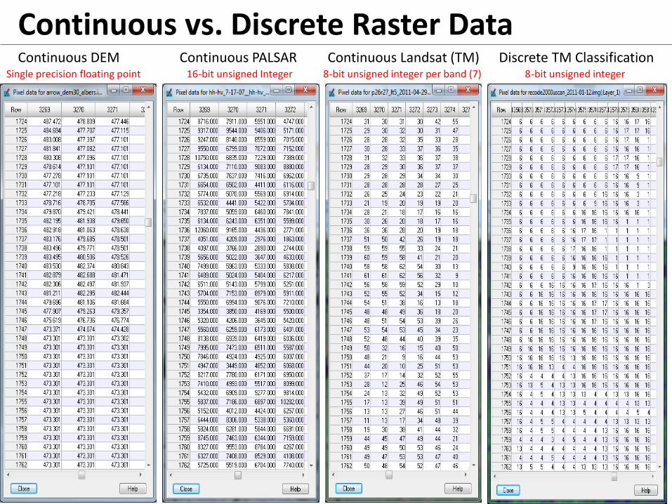
Single precision floating point 16-bit unsigned Integer 8-bit unsigned integer per band (7) 8-bit unsigned integer

Continuous DEM Continuous PALSAR Continuous Landsat (TM) Discrete TM Classification

Discrete (or Categorical) Raster Data Discrete TM Classification Columns (X)

Ro

ws

(Y)

Surface vs. Feature • Features are attributes (name, color, size, etc) given to a point, line, or a polygon • Surface is a term used in GIS to define a raster layer (DEM, rainfall, etc.)

• represent phenomena that have values at every point across their extent. • And, shows how continuous data can change

• These values are often derived from a limited set of sample values, either….

• based on direct measurement… • Gold/silver ore concentrations from sample locations • Surface temperature values from a network of weather reporting stations

• Or, mathematically derived from other data…

• slope & aspect surfaces derived from an elevation surface • surface of distances from bus stops in a city • surfaces showing concentration of criminal activity or probability of lightning

strikes.

• In the point sampling case (without ancillary data), values between points are often estimated by interpolation (leans heavily on assumption of spatial autocorrelation)

• Or, modeled using ancillary data – relationships between point data & ancillary data (e.g., satellite data).

Surface: Interpolation & Modeling

Surfaces are often depict probabilities…

Probability of an archeological site being near a stream

Probability of a bobolink occurrence modeling based on sampling + habitat

Probability of deer infection by CWD sample data…cause remains a mystery

Estimated Ozone Depletion Surface

Point-based Interpolation Surface Point-based + ancillary data modeled surface

Surface: Spatial Modeling

POINT SAMPLING DATA (120 plots) Canopy Diameter Crown Closure DBH Length of Live Crown Tree Height Basal Area

ANCILLARY DATA Multi-spectral Satellite data

MODEL Linear relationships between point data & reflectance at those points

SPATIAL ESTIMATION Apply model to all other pixels locations

Problems Best Suited to Raster GIS Data

When one is dealing with continuous phenomena with out exact boundaries Ex: Spread of oil pollutants from a point source over time…

Problems Best Suited to Raster GIS Data

Spread of air-borne pollutants from a point source over time…

…continuous phenomena with out exact boundaries.

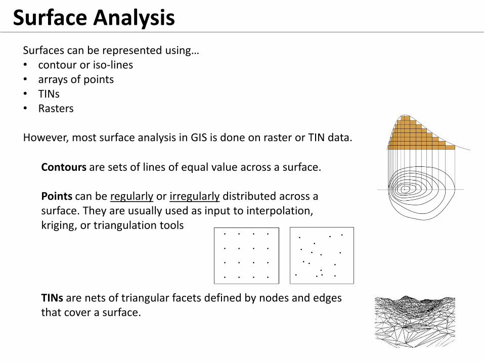
Surface Analysis Surfaces can be represented using… • contour or iso-lines • arrays of points • TINs • Rasters

However, most surface analysis in GIS is done on raster or TIN data.

Contours are sets of lines of equal value across a surface. Points can be regularly or irregularly distributed across a surface. They are usually used as input to interpolation, kriging, or triangulation tools TINs are nets of triangular facets defined by nodes and edges that cover a surface.

Contouring

Min 185m, Max 690m, Interval 25m

Interpolation Methods • Inverse Distance Weighting (IDW)

• Determines missing values via a linearly weighted combination of sample points N (Arc’s Default N = 12). • Closer sample point neighbors are given greater weight. • Interpolated surface should be that of a locationally dependent variable

• values depend on spatial location elevation, surface temperature etc.

• u(x) = interpolated value, u, at some point, x, … • based on i = 0,…,N samples ui = u(xi) • the distance weight function wi(x) • Where p is the power parameter

Where

• Splines (Bspline, Bezier, Cubic,…) • Estimates grid cell values by fitting a minimum-curvature surface to the sample data. • Like a flexible sheet of plastic that passes through each data point.

• But, bends as little as possible • TENSION option is more ridged and considered more realistic than the REGULARIZED (integrated average)

option in ArcGIS. • Cubic spline is common due to smoothness of curve pieces (between 2 points) • The spline function for each piece is defined as…

With coeficients 𝑎𝑖 𝑏𝑖 𝑐𝑖 to be determined by solving the governing continuity on each spline boundary… …which involves approximating the first derivative of each piece between points 𝒙 and 𝒙𝒊

• Natural Neighbors • Surface created using a neighbor technique via a weighted average of sample points. • Surface will not exceed MIN or MAX of sample data

Interpolation Methods

𝑆𝑖 = 𝑎𝑖 + 𝑏𝑖 (𝑥 − 𝑥𝑖) + 𝑐𝑖 (𝑥 − 𝑥𝑖)2

Interpolation Methods • Natural Neighbors – based on Voronoi tessellations

• Surface created using a neighbor technique via a weighted average of

sample points. • Surface will not exceed MIN or MAX of sample data

• Colored circles represent interpolating weights 𝒘𝒊 that are calculated based on the ratio of the shaded area to that of the cell area of the surrounding points.

• Basic 2D equation is: 𝐺 𝑥, 𝑦 = 𝑤𝑖𝑛𝑖=1 ∗ 𝑓(𝑥𝑖 , 𝑦𝑖)

• Where: 𝐺 𝑥, 𝑦 is the estimate at (𝑥𝑖 , 𝑦𝑖) • And: 𝑓(𝑥𝑖 , 𝑦𝑖) are the known data at (𝑥𝑖 , 𝑦𝑖)

Voronoi tessellations (Euclidean distances)

Interpolation Methods

• Kriging (uses spatial autocorrelation) • Sort of like IDW, but Kriging is more

sophisticated

• Centered around the idea that point sample that are closer in space tend to be more correlated that distant points. (Gold Mining)

• Interpolates surfaces based on weights inferred from the spatial structure of the input data (via a SEMI-VARIOGRAM)

• Things that are closer in space tend to be more correlated SPATIAL AUTOCORRELATION

Semi-Variograms

Semivariogram(distance h) = 0.5 * average [ (value at location I – value at location j)2]

Spherical Circular Gaussian Exponential

c

a

co

co + c

A = range

Semi-variogram parameters

c

a

co

co + c

• a = the range parameter, and is the distance limit of spatial autocorrelation… That is,

points farther than this distance are not correlated at all.

• Co = the nugget parameter, and is variability between spatially close points that is

not related to distance. Is either error in measurement or some other variability….originally corresponded to presence of gold deposits… hence, “nugget.”

• Co + C = the sill parameter, and is equivalent to the over all variance in you data

points.

• C = Distance from the nugget to the SILL

Semivariogram{@ some Lag distance h} = 0.5 * average [ (value at location X – value at location [Xi + h])2]

• Lag (h) = the distance between

pair of sample points being measured. For example, in remote sensing this would be…

• h=1 1 pixel separation • h=2 2 pixel separation • h=43 43 pixel separation….

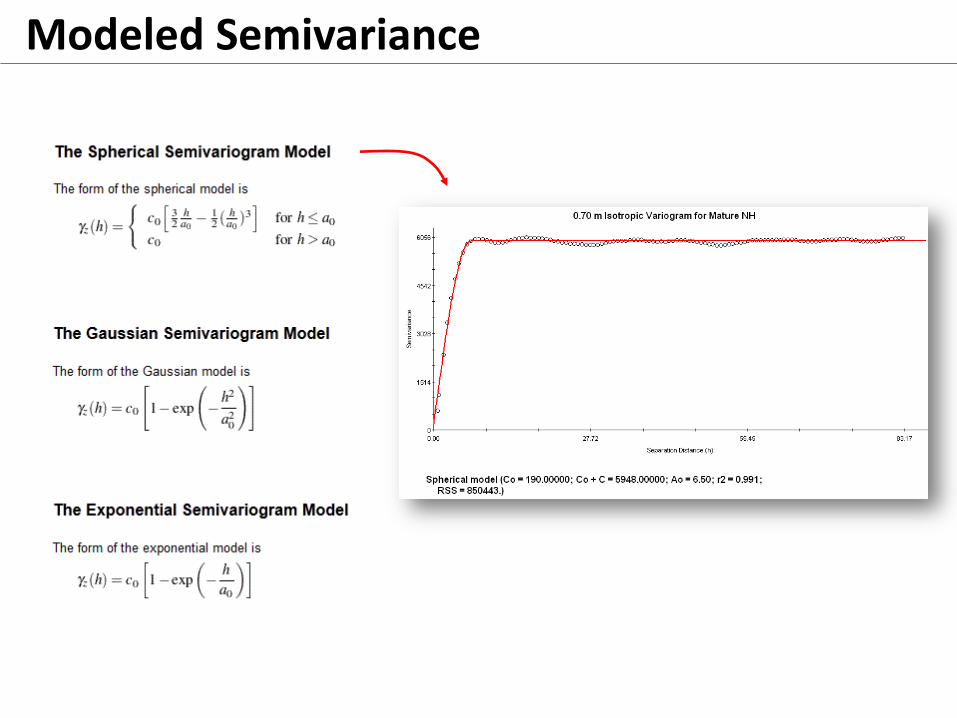
Modeled Semivariance

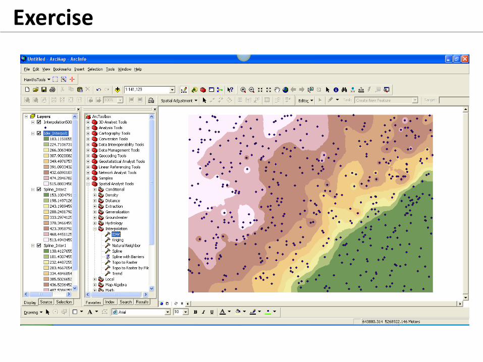
Exercise Min = 183 m Max = 690 m 500 sample points

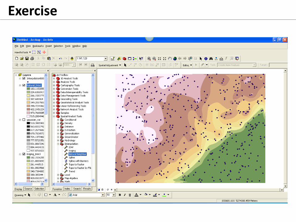
Exercise Modeled Semivariogram of the 500 sample points (Gaussian Model) Range (a) = 14.67km Sill (C + Co) variance = 32,300 (or a Standard Deviation of 179.7 m) Nugget (Co) = 600 m

Exercise

Exercise

Exercise

Exercise