Week 8: Fiscal policy in the New Keynesian

Model

Bianca De Paoli

November 2008

1 Fiscal Policy in a New Keynesian Model

1.1 Positive analysis: the e¤ect of �scal shocks

� How do �scal shocks a¤ect in�ation?

� Current economic environment: US �scal stimulus.

� See Summers & Calvo discussion (blog FT.com)

� UK potential �scal stimulus.

� "Fiscal Policy should be used when constrained Monetary Policy cannotreact to fall in activity"

� "Treasury �scal stimulus would prevent central bank to lower rates"

� Can �scal policy be used as an instrument to boost economic activity?

� What are the implications for in�ation?

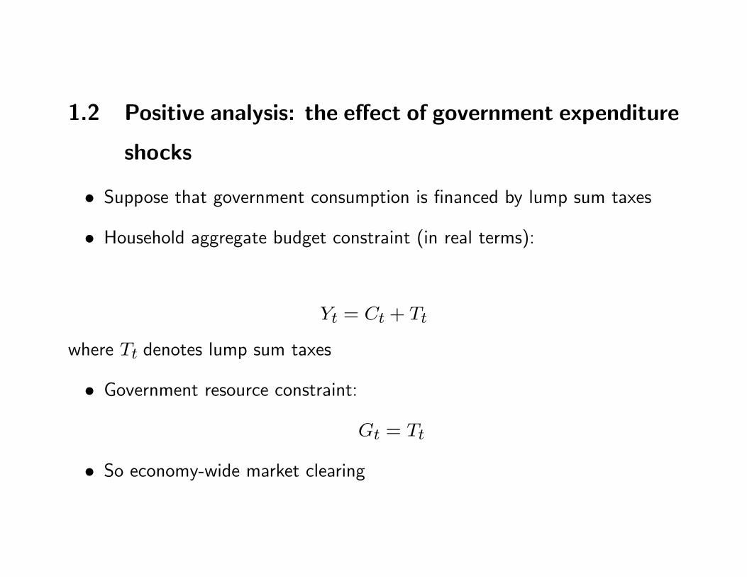
1.2 Positive analysis: the e¤ect of government expenditure

shocks

� Suppose that government consumption is �nanced by lump sum taxes

� Household aggregate budget constraint (in real terms):

Yt = Ct + Tt

where Tt denotes lump sum taxes

� Government resource constraint:

Gt = Tt

� So economy-wide market clearing

Yt = Ct +Gt

� The economy-wide resource constraint is given by

byt = (1� sg)bct + sgbgtwhere sg = G=Y . (slightly di¤erent speci�cation than in previous lec-tures)

� If one wants to allow for zero steady-state government consumption - de�neegt = (Gt �G)=Y = Gt=Y -then obtain

byt = bct + egt

The supply side e¤ect

� For any given level of output, �scal policy crowds out private consumption

� Lower consumption implies higher marginal utility of consumption

��bct = ��byt + �egt� Higher marginal utility implies higher labour supply and lower real marginalcost

� Total cost (constant returns Yt = Nt)

WtNt =WtYt

� Marginal cost is Wt, so real marginal cost, in log terms

dmct = bwt � bpt = �bct + 'bnt= (� + ')byt � �egt

� higher labour supply/lower marginal cost implies higher potential output

� With �exible prices, marginal cost is constant

bynt = �

� + 'egt

With sticky prices, the Phillips curve would be given by the usual equation

�t = �eyt + �Et�t+1

The demand side e¤ect

� As we have seen

byt = bct + egt� The Euler equation

bct = Etbct+1 � ��1(bit � Et�t+1)

becomes

byt � egt = Et(byt+1 � egt+1)� ��1(bit � Et�t+1)

or

eyt = Eteyt+1 � ��1(bit � Et�t+1 � brnt )where brnt = � �'

� + 'Et�egt+1

� So, a �scal shock (egt) increases the natural interest rate.� Fiscal shock increases aggregate demand.

� ...But it also increases supply.

� The net e¤ect on in�ation depends on the central bank response.

� Can you already infer the policy prescription of a central bank thatwants to maintain price stability?

� This is given by brnt : the interest rate that is consistent with constantprices increases after an increase in g.exp. => so, the central bankthat wants to maintain in�ation has to raise interest rates to containthe increase in demand and in�ationary pressures

10 20 30 40

­0.4

­0.2

0c

10 20 30 400

1

2g

10 20 30 400

0.05

0.1i

10 20 30 400

0.02

0.04pi

10 20 30 400

0.05r

10 20 30 400

0.05

0.1rn

10 20 30 400

0.5

1y

10 20 30 400

0.02

0.04ygap

10 20 30 400

0.5

1yn

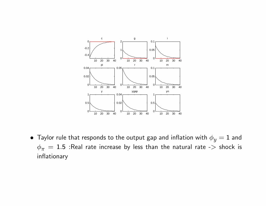
� Taylor rule that responds to the output gap and in�ation with �y = 1 and�� = 1:5 :Real rate increase by less than the natural rate -> shock isin�ationary

� Exercise:

� (A) Assume that the shock is iid.� A.1) Derive the reduce form solution for interest rates and in�ation asa function of the shock

� A.2) How does this interest rate rule compared with one which guar-antees price stability?

� A.3) Show that the larger �� the larger is the interest rate response tothe shock and the lower is the in�ation level.

� (B) Assume that the shock is an AR(1) with coe¢ cient � = 0:9 and codethe model in Dynare or Matlab

� Is it still the case that the larger �� the larger the nominal interest rateresponse? What about in�ation?

� Can you explain this result?

1.3 Positive analysis: the e¤ect of income tax shocks

� What are the e¤ects of income taxes?

� Suppose that the government taxes income and redistribute in lump sumtransfers

� Government budget constraint:

� �tYt = Tt

where � �t denote income taxes

� Aggregate household budget constraint:

(1� � �t)Yt + Tt = Ct

� Aggregate resource constrain in log linear terms:

Yt = Ct and byt = bct

� Taxes will a¤ect agent�s labour leisure decision

maxUt = Et

1Xs=t

�s�t24C1��s

1� �� N

1+'s

1 + '

35 ;subject toZ 1

0Ct (j)Pt (j) dj +QtBt � Bt�1 + (1� � �t)WtNt � Tt

� it decreases the supply of labour for each unit of real wage

�Un(Ct;Nt)Uc(Ct;Nt)

= (1� � �t)Wt

Pt

� This, ceteris paribus, increases real marginal cost

dmct = bwt � bpt = �bct + 'bnt + � �t

for simplicity we also assumed that taxes are zero in steady state

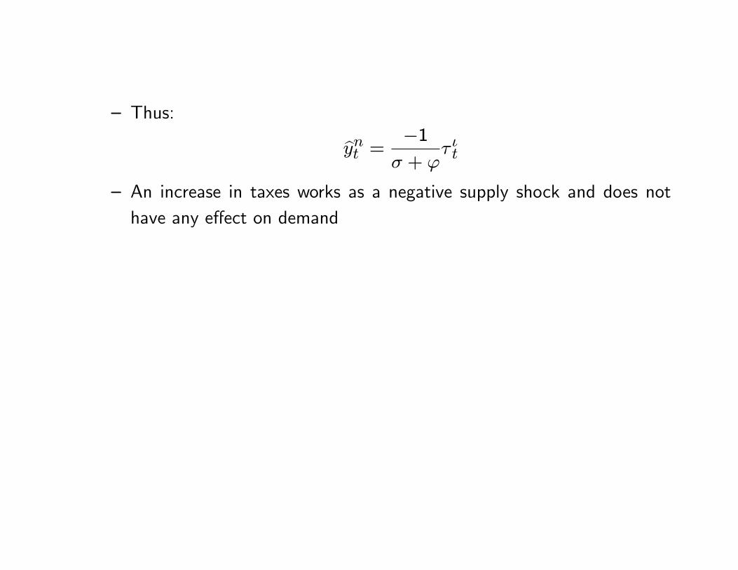
� Thus:

bynt = �1� + '

� �t

� An increase in taxes works as a negative supply shock and does nothave any e¤ect on demand

1.4 Positive analysis: �scal policy

� What are the e¤ects of government spending �nance by income taxes?

� Government budget constraint:

� �tYt = Gt

maintaining the zero-state assumptions

� �t = egt� Aggregate household budge constraint:

(1� � it)Yt = Ct

� So economy-wide market clearing in log linear terms

byt = bct + egt

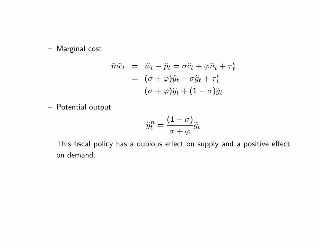
� Marginal cost

dmct = bwt � bpt = �bct + 'bnt + � �t

= (� + ')byt � �egt + � �t

(� + ')byt + (1� �)egt� Potential output

bynt = (1� �)

� + 'egt

� This �scal policy has a dubious e¤ect on supply and a positive e¤ecton demand.

1.5 Normative analysis: Fiscal Policy and Welfare

� Policy instruments: Public spending, Lump-sum taxes, Income taxes, In-�ation tax

� In�ation may be viewed as a tax from di¤erent points of view

� government can �nance their expenditure via seigniorage

� or in�ation can de�ate the real value of public debt, improving its�nancing conditions

� But which tax is more costly? In�ation tax, income tax, etc.

� Income taxes are costly because they a¤ect agents labour leisure decision(distort the incentives of agents to work an extra hour)

� Lump sum transfers are not costly, but are they feasible? Are they equi-table?

� In an NK model, in�ation is costly due to nominal rigidities

1.6 Normative analysis: Fiscal Policy and Welfare

1.6.1 What have we learned?

� Production Subsidy can improve welfare (Steady-state analysis)

� E¢ cient allocation

�UnUc

=MPNt

� We know that monopolistic competition may lead to lower production(suboptimal employment):

P =M W

MPN

�UnUc

=W

P=MPN

M

� Production subsidy �s can increase production towards e¢ cient level

�UnUc

=W

P=

MPN

(1� �s)M

� An income subsidy can increase labour supply towards it�s e¢ cient level

1.7 Normative analysis: Fiscal Policy and Welfare

1.7.1 What have we learned?

� Apart from the steady state analysis: changes in government spendingmay introduce a trade-o¤ between output and in�ation when steady stateis ine¢ cient

� the policymaker�s problem:

minE0

1Xk=0

�kh" (�t)

2 + � (~ywt )2i

s.t

�t = �eyt + �Et�t+1

� but the welfare relevant output gap is ~ywt = yt � ytt, where

ytt =d�gt

('+ �)6= ynt (1)

� Intuition: �scal shock can reduce monopolist distortion (because, as we�veseen, it increases potential output)

1.8 Normative analysis: Fiscal Policy and Welfare

1.8.1 Optimal �scal policy

� Up to now we have looked as �scal policy either in steady-state or as ashock

� What about formulating an endogenous feedback rule for the �scal instru-ment: ie how should taxes respond to shocks

� what �scal instrument: lump-sum taxes not realistic

� state contingent income taxes?

� But income taxes are discretionary

� The neoclassical literature on optimal �scal policy has suggested that, whentaxes are discretionary, welfare would be maximized if taxes are smoothed

over time and across states of nature (see Barro, 1979 and Lucas andStokey, 1983).

� In these models, if possible, taxes would be essentially invariant (see Lucasand Stokey, 1983 and Chari, Christiano and Kehoe, 1991)

� or would follow a random walk (see Barro, 1979, Aiyagari et al. 2002) whenthe �scal authority is forced to move taxes to adjust its public �nances

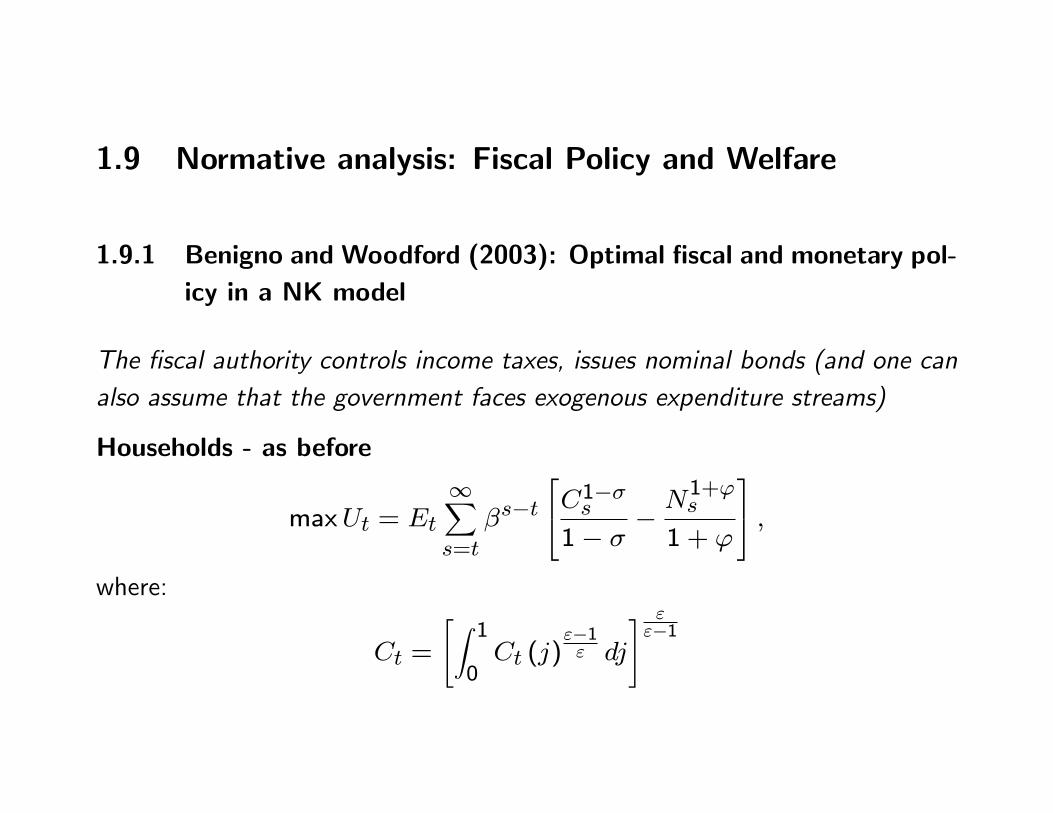
1.9 Normative analysis: Fiscal Policy and Welfare

1.9.1 Benigno and Woodford (2003): Optimal �scal and monetary pol-icy in a NK model

The �scal authority controls income taxes, issues nominal bonds (and one canalso assume that the government faces exogenous expenditure streams)

Households - as before

maxUt = Et

1Xs=t

�s�t24C1��s

1� �� N

1+'s

1 + '

35 ;where:

Ct =

"Z 10Ct (j)

"�1" dj

# ""�1

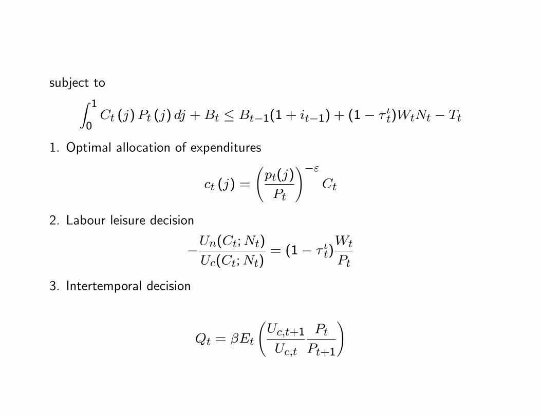
subject toZ 10Ct (j)Pt (j) dj +Bt � Bt�1(1 + it�1) + (1� � �t)WtNt � Tt

1. Optimal allocation of expenditures

ct (j) =

pt(j)

Pt

!�"Ct

2. Labour leisure decision

�Un(Ct;Nt)Uc(Ct;Nt)

= (1� � �t)Wt

Pt

3. Intertemporal decision

Qt = �Et

Uc;t+1

Uc;t

Pt

Pt+1

!

Firms- as before

� Optimal Price Setting

Xk

Et�kQt:t+kYt+k;t

hP �t �M t+k;t

i= 0

� Aggregate price dynamics

Pt =h� (Pt�1)

1�" + (1� �)P �1�"t

i 11�"

1.10 Government budget constraint

� the government issues one period nominal risk free bonds

� and collects taxes

� Government debt Dnt , expressed in nominal terms, follows the law of mo-

tion:

Dt = Dt�1(1 + it�1)� Pt�itYt

Or, we can de�ne

dt �Dt(1 + it)

Pt;

in order to rewrite the government budget constraint as

dt = dt�1(1 + it)

�t� � itYt(1 + it)

� In�ation reduces the real value of government debt

2 A log-linear representation of the model

� Phillips Curve

�t = � (�bct + 'byt + !b� �t � (1 + ')bat) + �Et�t+1

� as in the case of income taxes we�ve talked about, but here we allow fornon-zero steady state taxes, so ! = �=(1� �)

� Resource constraintbyt = bct

� IS curvebct = Etbct+1 � ��1(bit � Et�t+1)

� Government budget constraint (de�ning edt � (dt�d)=Y and dss = d=Y )

edt� = edt�1 � dss�t + dss�bit � �(b� it + byt)

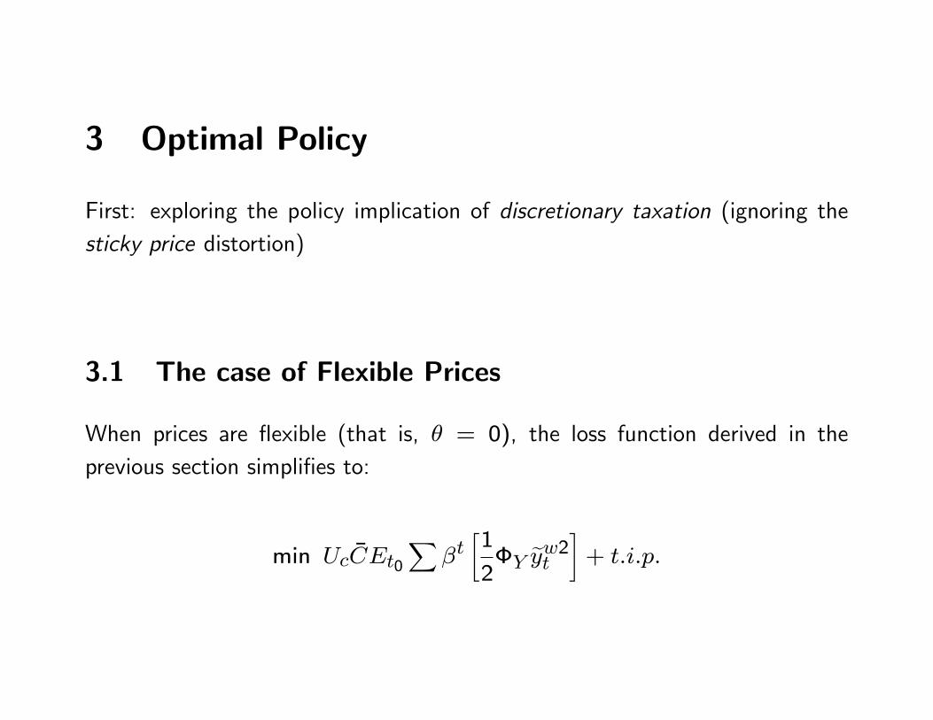
3 Optimal Policy

First: exploring the policy implication of discretionary taxation (ignoring thesticky price distortion)

3.1 The case of Flexible Prices

When prices are �exible (that is, � = 0), the loss function derived in theprevious section simpli�es to:

min Uc �CEt0X

�t�1

2�Y eyw2t �

+ t:i:p:

Alternatively, using the relationship between discretionary taxes and outputdictated by the Phillips curve, it is possible to rewrite the objective function as

min Uc �CEt0X

�t�1

2�� e� �w2t

�+ t:i:p+O(jj�jj3);

where �� = � !'+��Y

� Under this speci�cation, domestic producer in�ation is not costly (theassumption that � = 0 implies that �� = 0), and policymakers�incentivesare only a¤ected by tax distortions

� The constraints of the policy problem are given by the equilibrium condi-tions presented before

� Thus, the �rst order conditions implies that

eywt = e� �wt = 0:

� Since in�ation is not costly, optimal policy can induce unexpected varia-tions in domestic prices in order to restore �scal equilibrium.

� This result is consistent with the �ndings of Bohn (1990), Chari, Christianoand Kehoe (1991) and Benigno and Woodford (2003).

� Show that if debt is zero in steady state, i.e. dss = 0 the governmentcannot fully stabilize taxes

� Taxes vary across states but they remain constant after the shock hits theeconomy.

� The best policy available entails a "jump" in the tax rate in order to adjustthe level of primary surplus after the shock.

� Subsequently, taxes are kept constant as to minimize distortions in theconsumption/leisure trade-o¤. That is, the optimal plan implies

Et�eywt+1 = Et�e� �wt = 0:

(a similar rule would hold if dss 6= 0 but the government issued real bonds)

� Result consistent with Barro (1979)

3.2 The case of sticky prices

The policy problem

min Uc �CEt0X

�t�1

2�� ey�w2t +���

2t

�+ t:i:p+O(jj�jj3);

� Do not want to use in�ation to adjust the �scal conditions because in�ationis costly

� Although there are two policy incentives and two policy instruments - thatis, an active �scal and monetary policy - the �rst best cannot be achieved.

� It�s not possible to keep simultaneously in�ation and taxes constant acrossstates and over time.

� Nor is it possible, as in the �exible price case, to move tax rates perma-nently (and smooth them in subsequent periods).

� By inspection of the Phillips curve we note that, when prices are sticky,a permanent change in taxes would imply a non stationary process forin�ation (and an explosive path for the domestic price level).

� If we further assume that debt is zero in steady state, i.e. dss = 0, theoptimal plan implies

!Et�e� �wt + k�1���t = 0:

3.3 Open economy

Introduce another distortion... optimize the use of instruments...

Lito = Uc �CEt0X

�t�1

2�Y by2t + 12�RScrs2t + 12��(b�Ht )2

�+ t:i:p; (2)

If we further assume that debt is zero in steady state, i.e. dss = 0, the optimalplan implies

�rsEt�frswt+1 + (1 + l)

�(1� �)�YEt�eywt+1 = 0;

and

Etb�Ht+1 = 0