week 2 numerical descriptive measures · rp. 1.000.000 but less than rp. 1.500.000 13 rp. 1.500.000...
TRANSCRIPT
Statistic for Business
Week 2
Numerical Descriptive Measures

Agenda
Time Activity
90 minutes Central Tendency
60 minutes Variation and Shape
30 minutes Exploring Numerical Data

Objectives
By the end of this class, student should be able to understand:
• How to measures central tendency in statistics
• How to interpret those central tendency measurements

Numerical Descriptive Measures
Central Tendency
Variation and Shape
Exploring Numerical
Data
Numerical Descriptive
Measures for a Population
The Covariance
and The Coefficient of Correlation

CENTRAL TENDENCY

Central Tendency
Mean
(Arithmetic Mean)
Median
Mode Geometric
Mean

Mean
Consider this height data:
160 157 162 170 168 174 156 173 157
What is the mean height?

Mean
Sample size
n
XXX
n
X
X n21
n
1i
i
Observed values
The ith value Pronounced x-bar

Mean
How about this data of business statistic’s students monthly spending:
What is the MEAN?
Monthly Spending Frequency
less than Rp. 500.000 2
Rp. 500.000 but less than Rp. 1.000.000 7
Rp. 1.000.000 but less than Rp. 1.500.000 13
Rp. 1.500.000 but less than Rp. 2.000.000 5

Mean
In this case we can only ESTIMATE the MEAN…
Keyword: “MIDPOINTS”
Spending Frequency
less than Rp. 500.000 2
Rp. 500.000 but less than Rp. 1.000.000 7
Rp. 1.000.000 but less than Rp. 1.500.000 13
Rp. 1.500.000 but less than Rp. 2.000.000 5

Estimated Mean
Midpoint Frequency Mid * f 250000 2 500000 750000 7 5250000
1250000 13 16250000 1750000 5 8750000
Total 27 30750000
𝐸𝑠𝑡𝑖𝑚𝑎𝑡𝑒𝑑 𝑀𝑒𝑎𝑛 =30750000
27= 1138888.89

Mean
The following is “Student A” Score:
What is the average score of “Student A”?
Course Credits Score
Business Math 3 60
English 2 80
Organization Behavior 3 100
Statistics 4 90
Operation Management 3 70

Mean
Consider these two sets of data:
A 150 152 154 155 155 155 155 155 155 157
Mean?
B 150 152 154 155 155 155 155 155 155 187
Mean?

Mean
155 156 157 150 151 152 153 154 187
154.3
155 156 157 150 151 152 153 154 187
157.3 Extreme
Value
A
B

It is DANGEROUS to ONLY use
MEAN in describing a data

Median
dataorderedtheinposition2
1npositionMedian

Median
Consider these two sets of data:
A 150 152 154 155 155 155 155 155 155 157
Median?
B 150 152 154 155 155 155 155 155 155 187
Median?

Median
155 156 157 150 151 152 153 154 187
155
155 156 157 150 151 152 153 154 187
155
A
B
154.3
157.3

Median
What is the median of this height data:
160 157 162 170 168 174 156 173 157
How about this data:
160 157 162 170 168 174 156 173 157 150

Median
How about this data of business statistic’s students monthly spending:
What is the MEDIAN?
Monthly Spending Frequency
less than Rp. 500.000 2
Rp. 500.000 but less than Rp. 1.000.000 7
Rp. 1.000.000 but less than Rp. 1.500.000 13
Rp. 1.500.000 but less than Rp. 2.000.000 5

Median
The MEDIAN group of monthly spending is Rp. 1.000.000 but less than
Rp. 1.500.000
Or ESTIMATE
the MEDIAN!!

Estimated Median
Estimated Median = Rp. 1.173.076,92
Monthly Spending Frequency
less than Rp. 500.000 2
Rp. 500.000 but less than Rp. 1.000.000 7
Rp. 1.000.000 but less than Rp. 1.500.000 13
Rp. 1.500.000 but less than Rp. 2.000.000 5

Estimated Median

Mode
What is the mode of this height data:
160 157 162 170 168 174 156 173 157
How about this data:
160 157 162 170 168 174 156 173 150

Mode
How about this data of business statistic’s students monthly spending:
What is the MODE?
Spending Frequency
less than Rp. 500.000 2
Rp. 500.000 but less than Rp. 1.000.000 7
Rp. 1.000.000 but less than Rp. 1.500.000 13
Rp. 1.500.000 but less than Rp. 2.000.000 5

Mode
The MODAL group of monthly spending is Rp. 1.000.000 but less than
Rp. 1.500.000
But the actual Mode may
not even be in that group!


Mode
Without the raw data we don't really know…
However, we can ESTIMATE the MODE

Estimated Mode
Estimated Mode = Rp. 1.214.285,72
Spending Frequency
less than Rp. 500.000 2
Rp. 500.000 but less than Rp. 1.000.000 7
Rp. 1.000.000 but less than Rp. 1.500.000 13
Rp. 1.500.000 but less than Rp. 2.000.000 5

Estimated Mode

Central Tendency
Central Tendency
Arithmetic Mean
Median Mode
n
X
X
n
i
i 1
Middle value in the ordered array
Most frequently observed value

EXERCISE

3.10
This is the data of the amount that sample of nine customers spent for lunch ($) at a fast-food restaurant:
4.20 5.03 5.86 6.45 7.38 7.54 8.46 8.47 9.87
Compute the mean and median.

3.12
The following data is the overall miles per gallon (MPG) of 2010 small SUVs:
24 23 22 21 22 22 18 18 26
26 26 19 19 19 21 21 21 21
21 18 29 21 22 22 16 16
Compute the median and mode.

GEOMETRIC MEAN

Compounding Data
Interest Rate
Growth Rate
Return Rate

Compounding Data
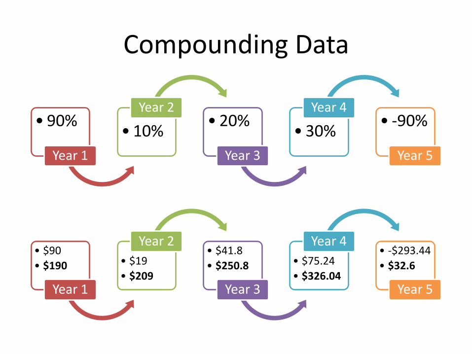
Suppose you have invested your savings in the stock market for five years. If your returns each year were 90%, 10%, 20%, 30% and -90%, what would your average return be during this period?

Compounding Data
• 90%
Year 1
• 10%
Year 2 • 20%
Year 3
• 30%
Year 4 • -90%
Year 5
If we use arithmetic mean in this case The average return during this period = 12%

Compounding Data
• 90%
Year 1
• 10%
Year 2 • 20%
Year 3
• 30%
Year 4 • -90%
Year 5
Let say that you invest $100 in year 0 How much your stocks worth in year 5?
Compounding Data
• 90%
Year 1
• 10%
Year 2 • 20%
Year 3
• 30%
Year 4 • -90%
Year 5
• $90
• $190
Year 1
• $19
• $209
Year 2 • $41.8
• $250.8
Year 3
• $75.24
• $326.04
Year 4 • -$293.44
• $32.6
Year 5

Geometric Mean
This is called geometric mean rate of return
11.03.12.11.19.15 GM
%08.20GM
Well, that’s pretty bad…

Measure of Central Tendency For The Rate Of Change Of A Variable Over Time:
The Geometric Mean & The Geometric Rate of Return
Geometric mean
Used to measure the rate of change of a variable over time
Geometric mean rate of return
Measures the status of an investment over time
Where Ri is the rate of return in time period i
n
nG XXXX /1
21 )(
1)]R1()R1()R1[(R n/1
n21G

Geometric Mean
1 n
ValueperiodofBeginning
ValuePeriodofEndGM

Geometric Mean
Lets reconsider the previous problem. We knew that we invest $100 in year 0 (zero). However, by the end of year 5 the value of the stock became $32.6. Calculate the annual average return!
•$100
Year 0
•$32.6
Year 5

Geometric Mean
• This value consistent with what we found earlier
1100
6.325 GM
%08.20GM

Population of West Java
Population of West Java:
• Year 2000: 35.729.537
• Year 2010: 43.053.732
Population growth rate per year?

3.22
In 2006-2009, the value of precious metals changed rapidly. The data in the following table represent the total rate of return (in percentage) for platinum, gold, an silver from 2006 through 2009:
Year Platinum Gold Silver
2009 2008 2007 2006
62.7 -41.3 36.9 15.9
25.0 4.3
31.9 23.2
56.8 -26.9 14.4 46.1

3.22
a. Compute the geometric mean rate of return per year for platinum, gold, and silver from 2006 through 2009.
b. What conclusions can you reach concerning the geometric mean rates of return of the three precious metals?

VARIATION AND SHAPE

Variation and Shape
Range
Variance and Standard Deviation
Coefficient of Variation
Z Scores
Shape

Review on Central Tendency
Consider this data:
160 157 162 170 168 174 156 173 157 150
What is the mean, median, and mode?

Range
Consider this data:
160 157 162 170 168 174 156 173 157 150
What is the Range?

Range
minmax XXRange

Measures of Variation: Why The Range Can Be Misleading
Ignores the way in which data are distributed
Sensitive to outliers
7 8 9 10 11 12
Range = 12 - 7 = 5
7 8 9 10 11 12
Range = 12 - 7 = 5
1,1,1,1,1,1,1,1,1,1,1,2,2,2,2,2,2,2,2,3,3,3,3,4,5
1,1,1,1,1,1,1,1,1,1,1,2,2,2,2,2,2,2,2,3,3,3,3,4,120
Range = 5 - 1 = 4
Range = 120 - 1 = 119

Variance and Standard Deviation
Variance Standard Deviation

Deviation
Let’s see this data again:
160 157 162 170 168 174 156 173 157 150
What is the mean?
Mean = 162.7

Deviation
Data Deviation 160 -2.7 157 -5.7 162 -0.7 170 7.3 168 5.3 174 11.3 156 -6.7 173 10.3 157 -5.7 150 -12.7
XXDeviation i
=156-162.7
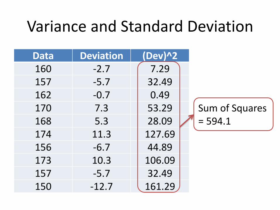
Variance and Standard Deviation
Data Deviation (Dev)^2 160 -2.7 7.29 157 -5.7 32.49 162 -0.7 0.49 170 7.3 53.29 168 5.3 28.09 174 11.3 127.69 156 -6.7 44.89 173 10.3 106.09 157 -5.7 32.49 150 -12.7 161.29
Sum of Squares = 594.1
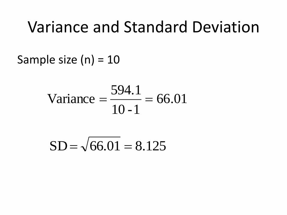
Variance and Standard Deviation
Sample size (n) = 10
01.661-10
594.1 Variance
125.866.01 SD

Variance and Standard Deviation
• Sample
• Population
1
1
2
2
n
XX
S
n
i
i
N
Xn
i
i
1
2
2

Measures of Variation: Comparing Standard Deviations
Mean = 15.5
S = 3.338 11 12 13 14 15 16 17 18 19 20 21
11 12 13 14 15 16 17 18 19 20 21
Data B
Data A
Mean = 15.5
S = 0.926
11 12 13 14 15 16 17 18 19 20 21
Mean = 15.5
S = 4.570
Data C

Standard Deviation
How about this data of business statistic’s students monthly spending:
What is the STANDARD DEVIATION?
Monthly Spending Frequency
less than Rp. 500.000 2
Rp. 500.000 but less than Rp. 1.000.000 7
Rp. 1.000.000 but less than Rp. 1.500.000 13
Rp. 1.500.000 but less than Rp. 2.000.000 5
E.S.T.I.M.A.T.I.O.N
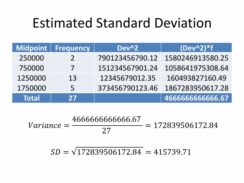
Estimated Standard Deviation
Midpoint Frequency Dev^2 (Dev^2)*f 250000 2 790123456790.12 1580246913580.25 750000 7 151234567901.24 1058641975308.64
1250000 13 12345679012.35 160493827160.49 1750000 5 373456790123.46 1867283950617.28
Total 27 4666666666666.67
𝑉𝑎𝑟𝑖𝑎𝑛𝑐𝑒 =4666666666666.67
27 = 172839506172.84
𝑆𝐷 = 172839506172.84 = 415739.71

THE COEFFICIENT OF VARIATION

The Coefficient of Variation
Height Weight

The Coefficient of Variation
Let’s see this height data again:
160 157 162 170 168 174 156 173 157 150
What is the mean and standard deviation
Mean = 162.7 and SD = 8.125

The Coefficient of Variation
Students with height before is weighted as follows:
50 55 57 52 55
69 60 65 71 70
What is mean and standard deviation?
Mean = 60.4 and SD = 7.8

The Coefficient of Variation
Height Weight
Mean 162.7 60.4
SD 8.125 7.8
Which one has more variability? Coefficient of Variation: CVHeight = 4.99% CVWeight= 12.92%

The Coefficient of Variation
%100.
X
SDCV

Locating Extreme Outliers: Z Score
Let’s see this height data again:
160 157 162 170 168 174 156 173 157 150
160 162 164 150 152 154 156 158
Mean = 162.7
166 168 170 172 174
SD = 8.125 SD = 8.125

Locating Extreme Outliers: Z Score
Therefore, Z Score for 160 is?
160 162 164 150 152 154 156 158
Mean = 162.7
166 168 170 172 174
Z Score162.7 = 0 Z Score154.6 = -1 Z Score170.8 = 1
SD = 8.125

Locating Extreme Outliers: Z Scores
Let’s see this height data again:
160 157 162 170 168 174 156 173 157 150
What is the Z Scores of 160, 174, 168 and 150?
Z160 = -0.33, Z174 = 1.39, Z168 = 0.65, and
Z150 = -0.56

Locating Extreme Outliers: Z Score
SD
XXZ X
• A data value is considered an extreme outlier if its Z-score is less than -3.0 or greater than +3.0.
• The larger the absolute value of the Z-score, the farther the data value is from the mean.

Shape
Let’s see this height data again:
160 157 162 170 168 174 156 173 157 150
160 162 164 150 152 154 156 158
Mean = 162.7
166 168 170 172 174
Median = 161 Right-Skewed
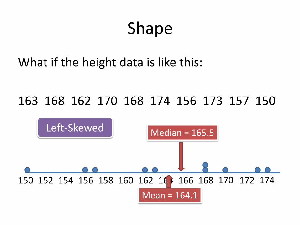
Shape
What if the height data is like this:
163 168 162 170 168 174 156 173 157 150
160 162 164 150 152 154 156 158
Mean = 164.1
166 168 170 172 174
Median = 165.5 Left-Skewed

Shape
Describes how data are distributed
Mean = Median Mean < Median Median < Mean
Right-Skewed Left-Skewed Symmetric

EXPLORING NUMERICAL DATA

Exploring Numerical Data
Quartiles
Interquartile Range
Five-Number Summary
Boxplot

Quartiles 1
st Q
uar
tile
Q1
2n
d Q
uar
tile
Q2
Median
3rd
Qu
arti
le
Q3

Quartiles
Let’s consider this height data:
160 157 162 170 168 174 156
What is the Q1, Q2 and Q3?
Q1 = 157
Q2 = 162 (Median)
Q3 = 170

Quartiles
Let’s then consider this height data:
160 157 162 170 168 174 156 173 150
What is the Q1, Q2 and Q3?
Q1 = 156.5
Q2 = 162 (Median)
Q3 = 171.5
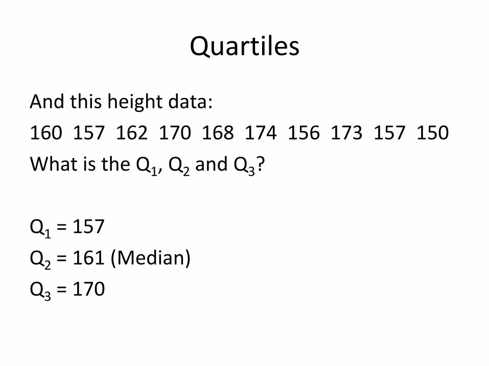
Quartiles
And this height data:
160 157 162 170 168 174 156 173 157 150
What is the Q1, Q2 and Q3?
Q1 = 157
Q2 = 161 (Median)
Q3 = 170

Quartiles
160 162 164 150 152 154 156 158
Median = 161
166 168 170 172 174
Q1 = 157 Q3 = 170
25% 25% 25% 25%
of all data

Interquartile Range
160 162 164 150 152 154 156 158 166 168 170 172 174
Q1 = 157 Q3 = 170
50%
In the middle of all data

Interquartile Range
160 162 164 150 152 154 156 158 166 168 170 172 174
Q1 = 157 Q3 = 170
What is the Interquatile range?
Interquartile Range = 170 – 157 = 13

Interquartile Range
13 QQRangeileInterquart

Five-Number Summary
max31min XQMedianQX

Five-Number Summary
Let’s see again this height data:
160 157 162 170 168 174 156 173 157 150
What is the Five-Number Summary?
150 157 161 170 174

Boxplot
Xmin Xmax Q1 Q3 Median

Boxplot
Let’s see again this height data:
160 157 162 170 168 174 156 173 157 150
Construct the Boxplot?

Boxplot for the Height of Business Statistic’s Student 2014
150 174 157 170 161
Height (cm)

Distribution Shape and The Boxplot
Right-Skewed Left-Skewed Symmetric
Q1 Q2 Q3 Q1 Q2 Q3 Q1 Q2 Q3

Karl Pearson's Measure of Skewness
160 162 164 150 152 154 156 158
Mean = 162.7
166 168 170 172 174
Median = 161
63.0125.8
)1617.162(3
kS

Karl Pearson's Measure of Skewness
S
MedianXSk
)(3

Bowley's Formula for Measuring Skewness
150 174 157 170 161
Height (cm)

Bowley's Formula for Measuring Skewness
)(
)()(
13
1223
QQQQSk

EXERCISE

3.10
This is the data of the amount that sample of nine customers spent for lunch ($) at a fast-food restaurant:
4.20 5.03 5.86 6.45 7.38 7.54 8.46 8.47 9.87
a. Compute the mean and median.
b. Compute the variance, standard deviation, and range
c. Are the data skewed? If so, how?
d. Based on the results of (a) through (c), what conclusions can you reach concerning the amount that customers spent for lunch?

3.62
In New York State, savings banks are permitted to sell a form of life insurance called savings bank life insurance (SBLI). The approval process consists of underwriting, which includes a review of the application, a medical information bureau check, possible requests for additional medical information and medical exams, and a policy compilation stage, during which the policy pages are generated and sent to the bank for delivery. The ability to deliver approved policies to customers in a timely manner is critical to the profitability of this service to the bank. During a period of one month, a random sample of 14 approved policies was selected, and the following were the total processing times

3.62
73 19 16 64 28 28 31 90 60 56 31 56 22 18
a. Compute the mean, median, first quartile, and third quartile.
b. Compute the range, interquartile range, variance, and standard deviation.
c. Are the data skewed? If so, how?
d. What would you tell a customer who enters the bank to purchase this type of insurance policy and asks how long the approval process takes?

3.22
In 2006-2009, the value of precious metals changed rapidly. The data in the following table represent the total rate of return (in percentage) for platinum, gold, an silver from 2006 through 2009:
Year Platinum Gold Silver
2009 2008 2007 2006
62.7 -41.3 36.9 15.9
25.0 4.3
31.9 23.2
56.8 -26.9 14.4 46.1

3.22
a. Compute the geometric mean rate of return per year for platinum, gold, and silver from 2006 through 2009.
b. What conclusions can you reach concerning the geometric mean rates of return of the three precious metals?

3.66
The table contains data on the calories and total fat (in grams per serving) for a sample of 12 veggie burgers.
Calories Fat 110 3.5 110 4.5 90 3.0 90 2.5
120 6.0 130 6.0 120 3.0 100 3.5 140 5.0 70 0.5
100 1.5 120 1.5

3.66
a. For each variable, compute the mean, median, first quartile, and third quartile.
b. For each variable, compute the range, variance, and standard deviation
c. Are the data skewed? If so, how?
d. Compute the coefficient of correlation between calories and total fat.
e. What conclusions can you reach concerning calories and total fat?

THANK YOU