wecc battery storage guideline - western electricity ... battery storage... · web viewwecc battery...

Western Electricity Coordinating Council Modeling and Validation Work Group

WECC Battery Storage Dynamic Modeling Guideline

Prepared by WECC Renewable Energy Modeling Task Force

November 2016

1

Contents

1. INTRODUCTION........................................................................................................3

2. BACKGROUND..........................................................................................................5

3. WECC BESS GENERIC MODELS FOR STABILITY STUDIES..............................................8

4. BESS MODEL SAMPLE SIMULATION.........................................................................22

5. REFERENCES............................................................................................................39

APPENIDX..............................................................................................................................41

A. PARAMETERS FOR REEC_C MODEL....................................................................................41

2

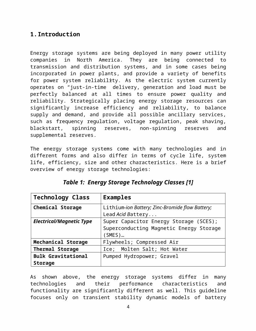
1. Introduction

Energy storage systems are being deployed in many power utility companies in North America. They are being connected to transmission and distribution systems, and in some cases being incorporated in power plants, and provide a variety of benefits for power system reliability. As the electric system currently operates on “just-in-time” delivery, generation and load must be perfectly balanced at all times to ensure power quality and reliability. Strategically placing energy storage resources can significantly increase efficiency and reliability, to balance supply and demand, and provide all possible ancillary services, such as frequency regulation, voltage regulation, peak shaving, blackstart, spinning reserves, non-spinning reserves and supplemental reserves.

The energy storage systems come with many technologies and in different forms and also differ in terms of cycle life, system life, efficiency, size and other characteristics. Here is a brief overview of energy storage technologies:

Table 1: Energy Storage Technology Classes [1]

Technology Class Examples

Chemical Storage Lithium-ion Battery; Zinc-Bromide flow Battery; Lead Acid Battery...

Electrical/Magnetic Type Super Capacitor Energy Storage (SCES); Superconducting Magnetic Energy Storage (SMES)…

Mechanical Storage Flywheels; Compressed AirThermal Storage Ice; Molten Salt; Hot WaterBulk Gravitational Storage Pumped Hydropower; Gravel

As shown above, the energy storage systems differ in many technologies and their performance characteristics and functionality are significantly different as well. This guideline focuses only on transient stability dynamic models of battery energy storage systems (BESS) which is one of many energy storage technologies widely adopted in the current power industry in North America. Modeling of other type of energy storage systems other than battery energy storage is out of the scope of this guideline. However, it should be noted that the primary aspect of the model developed in WECC [3], and discussed in this guideline, is the power inverter interface between the storage mechanism (battery) and the grid. Therefore, conceptually, this same model could potentially be applied for modeling other storage technologies, so long as the interface between the storage device and the grid is a power electronic, voltage source converter.

Among many battery energy storage technologies used in the power industry today are lithium-ion (LI) solid-state batteries, which is one of the most popular. Lithium-ion (LI) solid-state batteries have a broad technology class that includes many sub-types. Subtype classifications

3

generally refer to the cathode material. Lithium-ion technologies are also divided by cell shape: cylindrical, prismatic or laminate. Cylindrical cells have high potential capacity, lower cost and good structural strength. Prismatic cells have a smaller footprint, so they are used when space is limited (as in mobile phones). Laminate cells are flexible and safer than the other shapes. Its advantages include high energy density, high power, high efficiency, low self-discharge, lack of cell “memory” and fast response time while the challenges include short cycle life, high cost, heat management issues, flammability and narrow operating temperatures. Currently, approximate 70 battery energy storage systems with power ratings of 1 MW or greater are in operation around the world.

With more and more large-scale BESS being connected to bulk systems in North America, they play an important role in the system reliability. NERC Reliability Standards require that power flow and dynamics models be provided in accordance with regional requirements and procedures. Under the existing WECC modeling guidelines all aggregated generator plant with capacity 20 MVA or larger must be modeled explicitly in power flow and dynamics. And also, due to the difficulties associated with manufacturer-specific dynamic models, such as being proprietary in most cases, and portability across simulation platforms, standard generic models are preferred for bulk electric system studies. The NERC IVGTF (Integration of Variable Generation Task Force) Task 1-1 document explains that the term “generic” refers to a model that is standard, public and not specific to any vendor, so that it can be parameterized in order to reasonably emulate the dynamic behavior of a wide range of equipment. Furthermore, the NERC document, as well as working drafts of the documents from WECC REMTF and IEC TC88 WG27, explain that the intended usage of these models is primarily for power system stability analysis. Those documents also discuss the range in which these models are expected to be valid and the models’ limitations. As such, WECC requires the use of approved models, which are public (non-proprietary), available as standard-library models and have been tested and validated in accordance to WECC guidelines. Approved models are listed in the WECC Approved Dynamic Model List.

This document serves as a guideline for BESS generic dynamic models recently developed by WECC REMTF [3]. At the time of this guideline writing, there was no significant field test data available for us to validate this newly developed BESS model. REMTF is looking to BESS manufacturers and power utility companies for the possibility of field tests. Once such field test data is available the further update of BESS model and this document may be possible. Reference [8] does show the validation of the model for one case where field test data was available – this data was, however, covered under an NDA and so the data cannot be publicly shared. For any BESS projects, the user should always turn to the BESS manufacturer to verify the functionalities, parameters and models of their BESS. Furthermore, BESS modelling is an active research area and it continues to evolve with changes in technology and interconnection requirements, so BESS model validation against reference data remains a challenge due to limited industry experience.

4

Filter

Control and Protection

Operator and SCADA

1. Battery Cell Arrays 2. Power Conversion System 3. Control and Monitoring System

2. Background

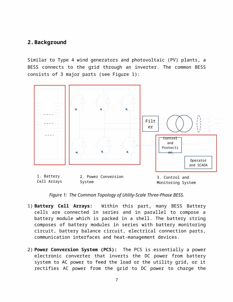
Similar to Type 4 wind generators and photovoltaic (PV) plants, a BESS connects to the grid through an inverter. The common BESS consists of 3 major parts (see Figure 1):

Figure 1: The Common Topology of Utility-Scale Three-Phase BESS.

1) Battery Cell Arrays: Within this part, many BESS Battery cells are connected in series and in parallel to compose a battery module which is packed in a shell. The battery string composes of battery modules in series with battery monitoring circuit, battery balance circuit, electrical connection parts, communication interfaces and heat-management devices.

2) Power Conversion System (PCS): The PCS is essentially a power electronic converter that inverts the DC power from battery system to AC power to feed the load or the utility grid, or it rectifies AC power from the grid to DC power to charge the battery system. The PCS operates according to the command of monitoring and control system.

3) Control and Monitoring System: The control circuit is the key part of the PCS. The part usually uses industrial-grade fast DSP (Digital Signal Processor) chipset as core processors. The function of Control Circuit includes: signal sampling, computing, PCS control, PCS

5

1st Quadrant

P>0Q>0

P<0Q>0

P<0Q<0

P>0Q<0

P=1Q=0

P=0Q=1

P= -1Q= 0

P= 0Q= -1

2nd Quadrant

3nd Quadrant 4th Quadrant

abnormality judgment and protection, communication with PCS HMI. From modeling aspects, it is the core of the functionality of the BESS and where voltage regulation, frequency regulation, and MW generation variations controls are implemented.

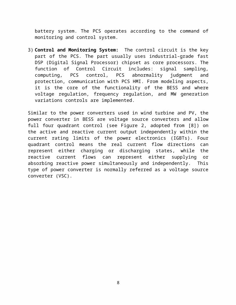
Similar to the power converters used in wind turbine and PV, the power converter in BESS are voltage source converters and allow full four quadrant control (see Figure 2, adopted from [8]) on the active and reactive current output independently within the current rating limits of the power electronics (IGBTs). Four quadrant control means the real current flow directions can represent either charging or discharging states, while the reactive current flows can represent either supplying or absorbing reactive power simultaneously and independently. This type of power converter is normally referred as a voltage source converter (VSC).

Figure 2: BESS Full Four Quadrant Control and Operation (adopted from [8])

By implementing various control strategies, the BESS can provide the following functionalities:

1. Voltage control and regulation at the local terminals of the BESS, at the point of interconnection (POI) or plant level (when incorporated in a power plant).

2. Frequency support by quickly providing or absorbing real power or being part of automatic generation control (AGC).

3. Spinning reserves, non-spinning reserves, or supplemental reserves. Generation capacity over and above customer demand is reserved for use in the event of contingency events like unplanned outages. Many storage technologies can be quickly synchronized to grid

6

frequency through power electronics control, so they can provide a service equivalent to spinning reserves with minimal to zero standby losses (unlike the idling generators). Energy storage is also capable of providing non-spinning or supplemental reserves.

4. Power oscillation damping. Although this is not a primary use of BESS, it can be used to damp or alleviate power oscillations if the proper supplemental controls are deployed, and the BESS is strategically located in the transmission system to be able to affect the modes of oscillation of concern. Low frequency inter-area power oscillations in the range below 2 Hz are a common phenomenon arising between groups of synchronous generators interconnected by weak and/or heavily loaded AC interties. Such oscillations can lead to stability problems if they are not adequately damped.

5. Reduce the net variability of variable generation resources, if combined with variable generation facilities such as wind or photovoltaics.

3. WECC BESS Generic Models for Stability Studies

3.1 Power Flow Representation

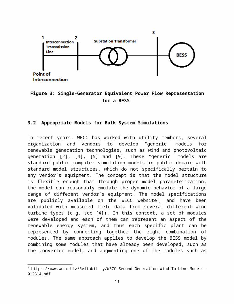
The WECC generic dynamic models described in this guideline assume that the BESS are represented explicitly in power flow, representing a single plant connected to transmission or distribution systems. Unlike wind and solar plants, the BESS plant is not widely spread out across an area, but is in modular containers. For example, the 2MW/4MWh BESS could include 4 sets of 40 feet modular containers. Therefore, there is no need to model a collector system, all that is needed to be modeled explicitly is the pad-mount and substation transformer, together with a single-generator equivalent model for the BESS, as shown in Figure 3.

Figure 3: Single-Generator Equivalent Power Flow Representation for a BESS.

7

3.2 Appropriate Models for Bulk System Simulations

In recent years, WECC has worked with utility members, several organization and vendors to develop “generic” models for renewable generation technologies, such as wind and photovoltaic generation [2], [4], [5] and [9]. These “generic” models are standard public computer simulation models in public-domain with standard model structures, which do not specifically pertain to any vendor’s equipment. The concept is that the model structure is flexible enough that through proper model parameterization, the model can reasonably emulate the dynamic behavior of a large range of different vendor’s equipment. The model specifications are publicly available on the WECC website1, and have been validated with measured field data from several different wind turbine types (e.g. see [4]). In this context, a set of modules were developed and each of them can represent an aspect of the renewable energy system, and thus each specific plant can be represented by connecting together the right combination of modules. The same approach applies to develop the BESS model by combining some modules that have already been developed, such as the converter model, and augmenting one of the modules such as REEC_B to REEC_C to model BESS. Section 3.3 will describe the generic BESS model structure in detail.

Those WECC generic models designed for transmission planning studies are to assess dynamic performance of the system, particularly recovery dynamics following grid-side disturbances such as transmission-level faults. In this context, WECC uses positive-sequence power flow and dynamic models that provide a good representation of recovery dynamics using integration time steps of one quarter cycle. This approach does not allow for detailed representation of very fast controls and response to imbalanced disturbances. The WECC whitepaper [2] lists the limitations of generic renewable energy system models, all of which equally applies to the BESS models being discussed here. .

3.3 BESS Generic Models Structures

Dynamic representation of a large-scale battery energy storage system for system planning studies requires the use of two or three new renewable energy (RE) modules shown below in Figure 4 [10][11]. These modules, in addition to others, are also used to represent wind and PV power plants.

1 https://www.wecc.biz/Reliability/WECC-Second-Generation-Wind-Turbine-Models-012314.pdf

8

Vref/Vreg or Qref/Qgen f/f_ref and Pgen/Pplant_ref

Plant ControllerREPC_A

Qref(or Qext)

Qgen

Pref

Q Control

P Control

Current LimitLogic

Iqcmd’

Ipcmd’

Iqcmd

Ipcmd

REGC_A

Generator/Converter

Model

Iq

Ip

Pqflag = 1 (P priority) = 0 (Q priority)

Vt

REEC_C

Pgen

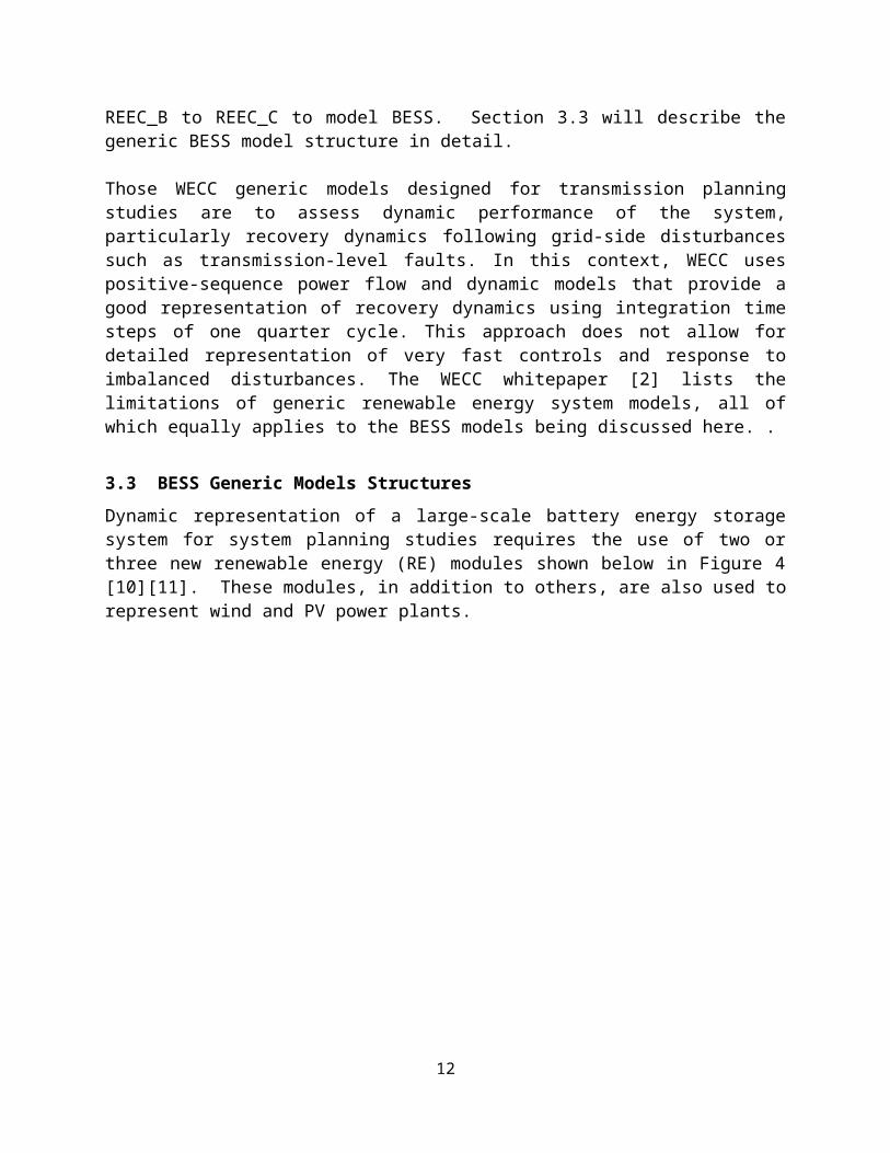
Figure 4: Block Diagram Representation of the BESS Model with the Plant Controller Optional.

1) REGC_A Module: Without modification, this module is used to represent the Battery/converter (inverter) interface with the grid. It takes in the real current command (Ipcmd) and the reactive current command (Iqcmd) from the main controls, and outputs of real (Ip) and reactive (Iq) current injected into the grid model. This module’s block diagram is shown in Figure 5. The details of “High Voltage Reactive Current Management” and “Low Voltage Active Current Management” can be found in Appendix D of Reference [9].

9

High Voltage Reactive Current

Management

Low Voltage Active Current

Management

-11+sTg

Iqrmax

Iqrmin

Iq

Iqcmd

Vt

Ip 1

1+sTg

LVPL & rrpwr

Ipcmd

11+sTfltr

LVPL

Lvpl1

Zerox Brkpt V

Lvplsw 0 1

InterfaceTo

NetworkModels

Figure 5: Block Diagram of Renewable Energy Generator/Converter Module (REGC_A) (source reference [9]).

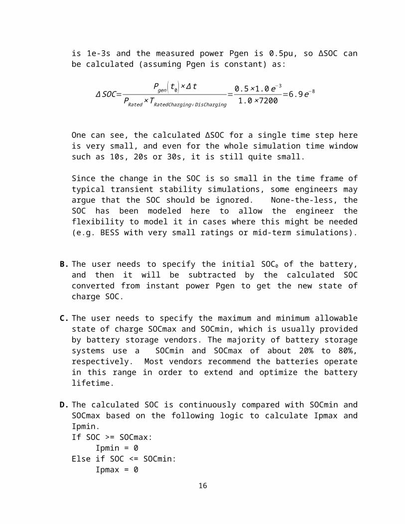
2) REEC_C Module: it is an augmented version of the existing renewable energy electrical control (REEC_A) model, which can be connected together in various combinations to yield a type 3, type 4 wind turbine generator or a photovoltaic (PV) system. As with the REEC_A model, it can be connected to the plant controller models REPC_A or REPC_B. REEC_C provides real (Ipcmd) and reactive (Iqcmd) current commands to the REGC_A module. The overall structure of Module REEC_C is shown in Figure 6. It should be noted that extreme care should be taken in coordinating the parameters dbd1, dbd2 and Vdip, Vup so as not to have an unintentional response from the reactive power injection control loop.

For REEC_C module is shown in Figure 6 (adopted from [3]) , the key augmented part is shown in red and represents a simple charging and discharging block of the battery storage. This key augmented part is also shown in Figure 7. The rest coming from REEC_A has no changed, with the exception of some simplifications in the current injection logic that was not relevant for this application.

10

Here is the highlight of this added block diagram representing the charging and discharging mechanism of the BESS:

A. This module counts on State of Charge (SOC) in both initial condition and the calculated SOC based on the real-time power output Pgen from the BESS. The SOC is defined as the available energy expressed as a percentage of the battery’s rated capacity. In the battery industry, the energy stored in a battery is more likely to be expressed as A*h, but this ambiguity can lead to confusion and errors. Rather than A*h, the energy stored in a battery should be expressed as W*h, kW*h, or MW*h. Given the above, in theory, State of Charge(SOC) should be calculated as:

SOC=EavailableERated

=Pavailable×T Charging∨DisChargingPRated×T Rated Charging∨DisCharging

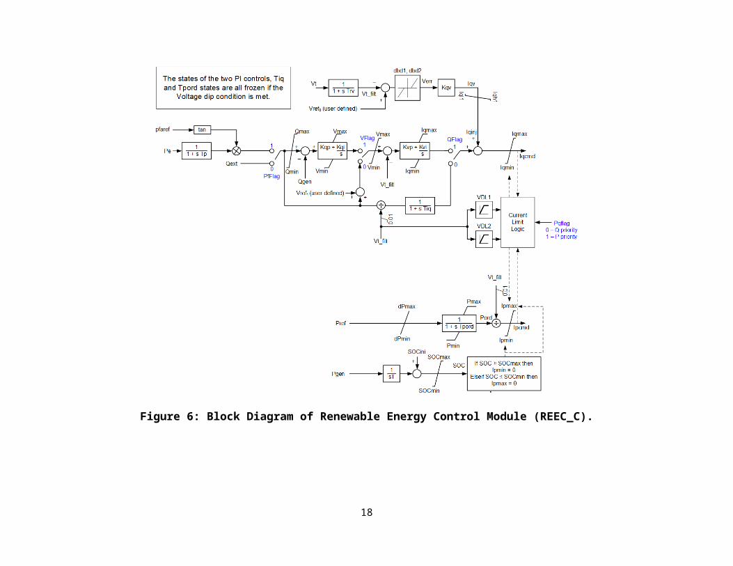
It is therefore easy to see that the change in the SOC can be simulated by simply taking the integral of the difference between the initial SOC and the current power being generated by the BESS, in the per unit system. This leads to the simple model shown in Figure 7.

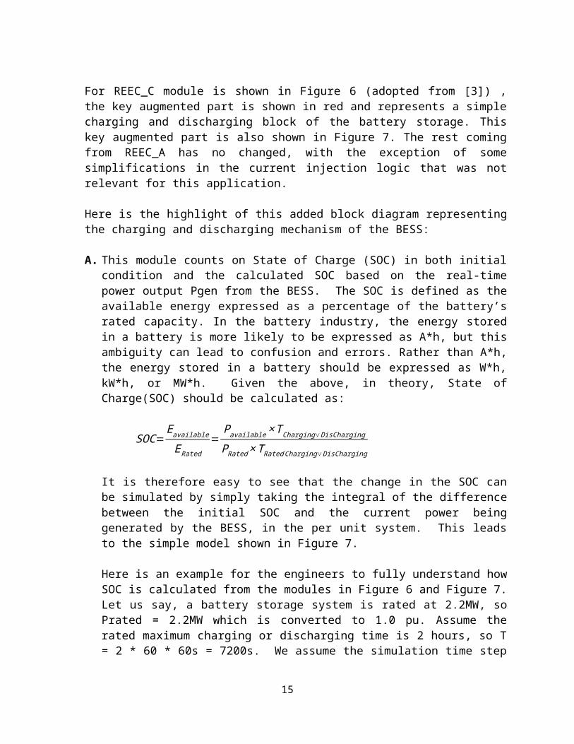
Here is an example for the engineers to fully understand how SOC is calculated from the modules in Figure 6 and Figure 7. Let us say, a battery storage system is rated at 2.2MW, so Prated = 2.2MW which is converted to 1.0 pu. Assume the rated maximum charging or discharging time is 2 hours, so T = 2 * 60 * 60s = 7200s. We assume the simulation time step is 1e-3s and the measured power Pgen is 0.5pu, so ΔSOC can be calculated (assuming Pgen is constant) as:

∆ SOC=Pgen (t 0 )×∆t

PRated×T Rated Charging∨DisCharging=0.5×1.0e−3

1.0×7200=6.9e−8

One can see, the calculated ΔSOC for a single time step here is very small, and even for the whole simulation time window such as 10s, 20s or 30s, it is still quite small.

Since the change in the SOC is so small in the time frame of typical transient stability simulations, some engineers may argue that the SOC should be ignored. None-the-less, the SOC has been modeled here to allow the engineer the flexibility to model it in cases where this might be needed (e.g. BESS with very small ratings or mid-term simulations).

B. The user needs to specify the initial SOC0 of the battery, and then it will be subtracted by the calculated SOC converted from instant power Pgen to get the new state of charge SOC.

11

C. The user needs to specify the maximum and minimum allowable state of charge SOCmax and SOCmin, which is usually provided by battery storage vendors. The majority of battery storage systems use a SOCmin and SOCmax of about 20% to 80%, respectively. Most vendors recommend the batteries operate in this range in order to extend and optimize the battery lifetime.

D. The calculated SOC is continuously compared with SOCmin and SOCmax based on the following logic to calculate Ipmax and Ipmin.If SOC >= SOCmax:

Ipmin = 0Else if SOC <= SOCmin:

Ipmax = 0

Ipmax and Ipmin is the maximum and minimum active current limit, respectively. By forcing these limits to zero when the battery’s SOC hits its limits, the BESS is then shut down so that it cannot further charge or discharge once at the SOCmax or SOCmin, respectively.

Please Note, from above module, one can see the battery chemistry is ignored, and also, the details of the dynamics of the dc current/voltage and three-phase AC current/voltage in converter/inverter are ignored in this model since they are not relevant to power system transient stability studies.

12

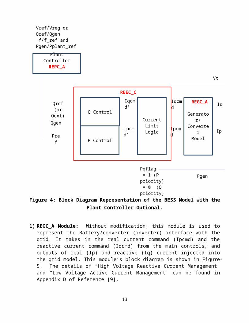
Figure 6: Block Diagram of Renewable Energy Control Module (REEC_C).

13

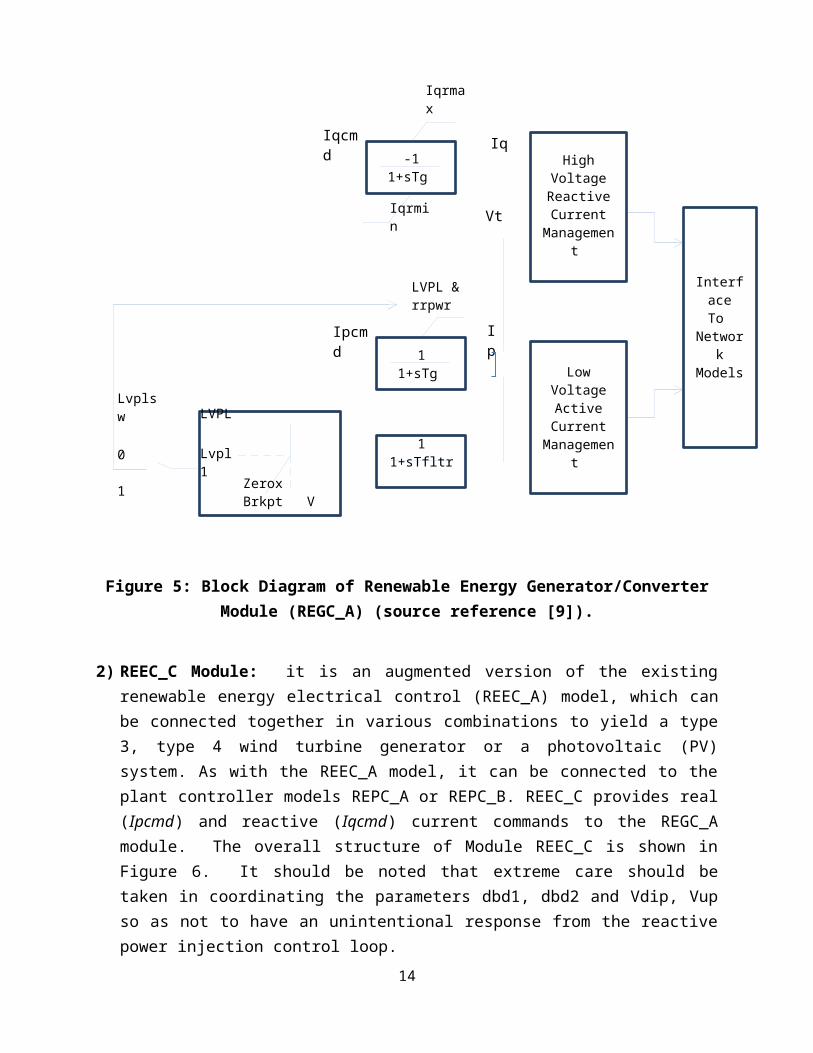
Figure 7: Block Diagram of the Charging/Discharging Mechanism of the BESS

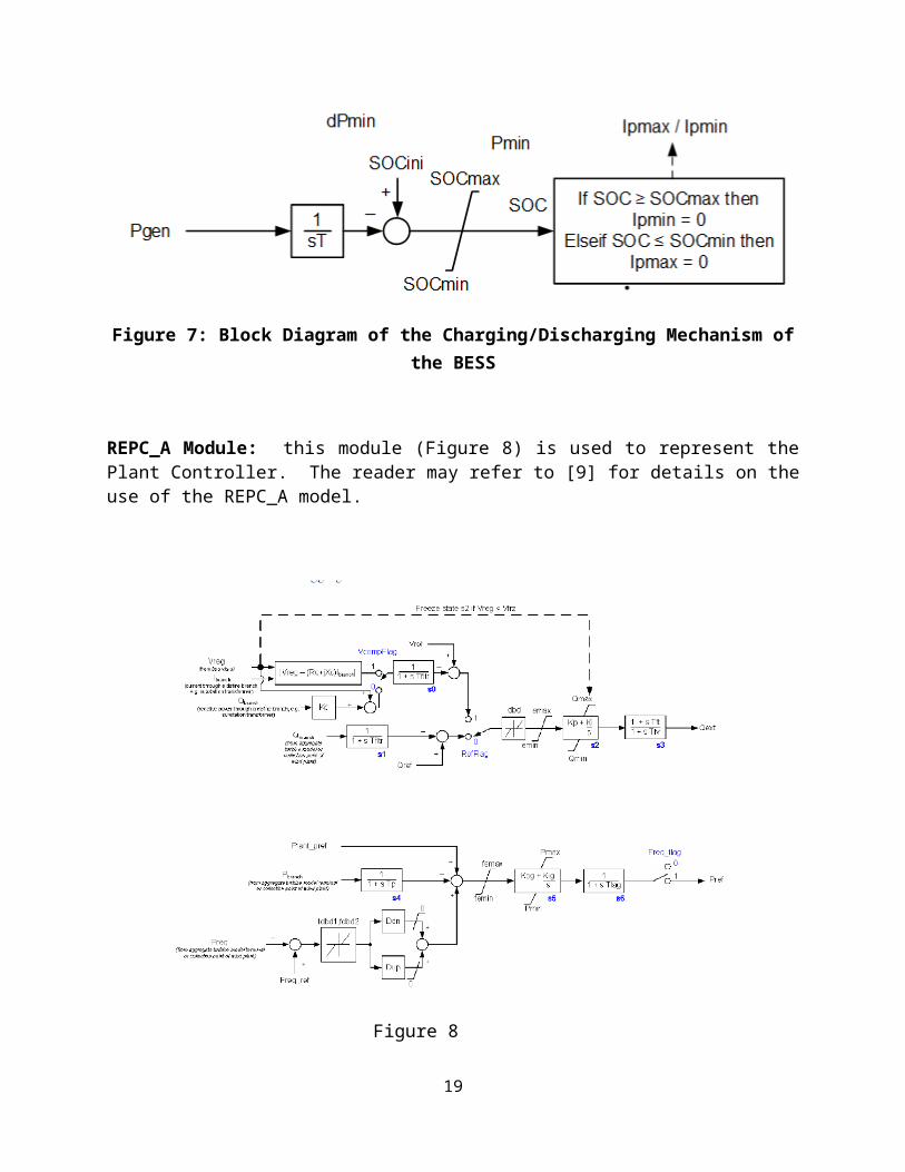
REPC_A Module: this module (Figure 8) is used to represent the Plant Controller. The reader may refer to [9] for details on the use of the REPC_A model.

Figure 8

14

3.4 BESS Generic Model Control Options

Similar to WECC Type 4 wind generator models and solar plant models, BESS models introduced above can have the following control options for reactive power and real power [4, 5, 9]:

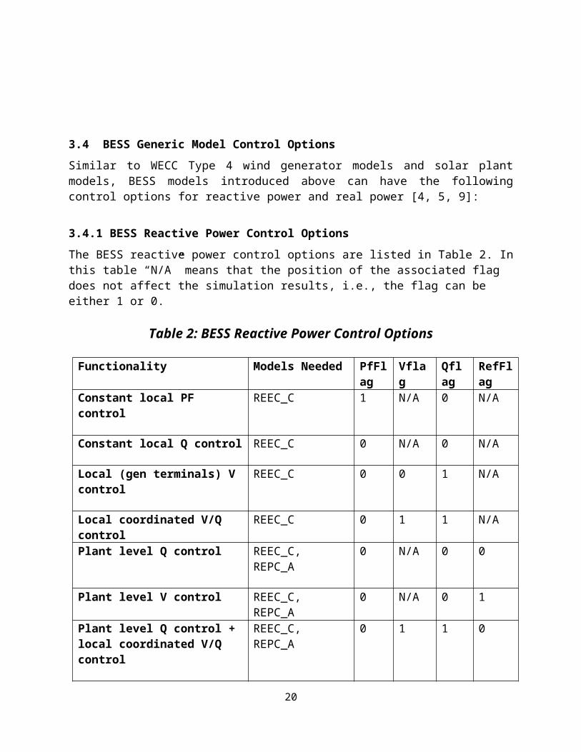
3.4.1 BESS Reactive Power Control Options

The BESS reactive power control options are listed in Table 2. In this table “N/A” means that the position of the associated flag does not affect the simulation results, i.e., the flag can be either 1 or 0.

Table 2: BESS Reactive Power Control Options

Functionality Models Needed PfFlag Vflag Qflag RefFlagConstant local PF control REEC_C 1 N/A 0 N/A

Constant local Q control REEC_C 0 N/A 0 N/A

Local (gen terminals) V control REEC_C 0 0 1 N/A

Local coordinated V/Q control REEC_C 0 1 1 N/A

Plant level Q control REEC_C, REPC_A 0 N/A 0 0

Plant level V control REEC_C, REPC_A 0 N/A 0 1

Plant level Q control + local coordinated V/Q control

REEC_C, REPC_A 0 1 1 0

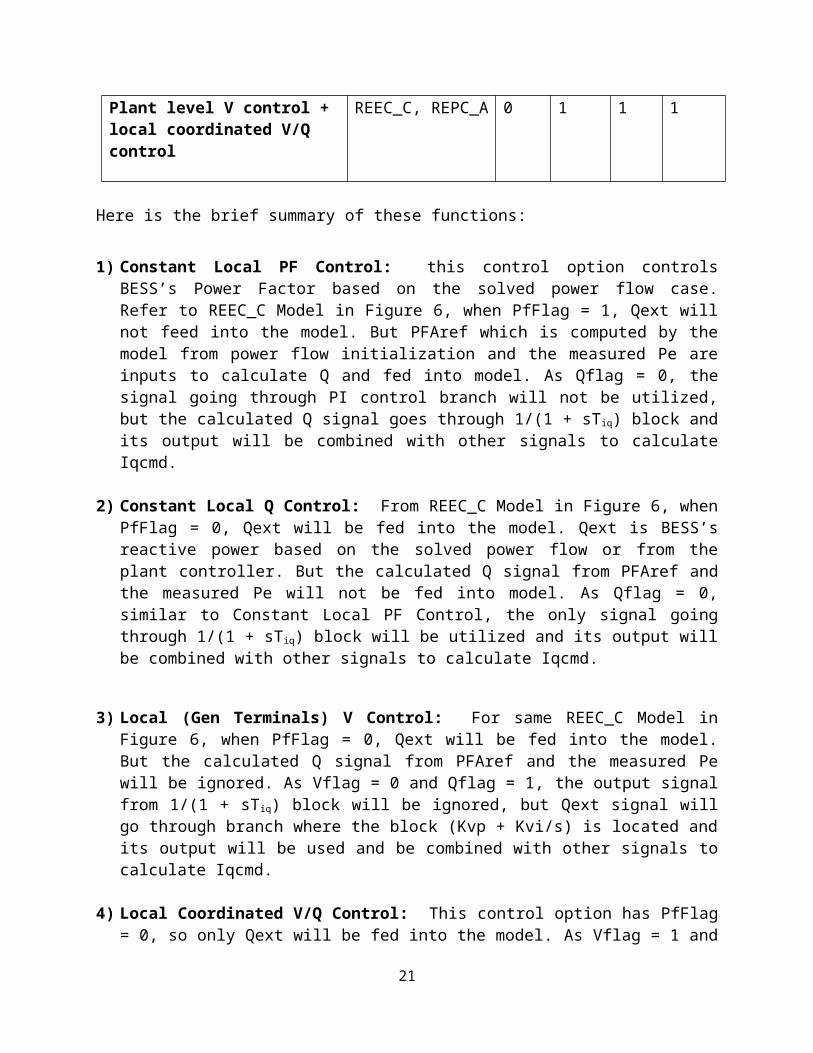
Plant level V control + local coordinated V/Q control

REEC_C, REPC_A 0 1 1 1

Here is the brief summary of these functions:

1) Constant Local PF Control: this control option controls BESS’s Power Factor based on the solved power flow case. Refer to REEC_C Model in Figure 6, when PfFlag = 1, Qext will not feed into the model. But PFAref which is computed by the model from power flow initialization and the measured Pe are inputs to calculate Q and fed into model. As Qflag = 0, the signal going through PI control branch will not be utilized, but the calculated Q signal goes through 1/(1 + sTiq) block and its output will be combined with other signals to calculate Iqcmd.

15

2) Constant Local Q Control: From REEC_C Model in Figure 6, when PfFlag = 0, Qext will be fed into the model. Qext is BESS’s reactive power based on the solved power flow or from the plant controller. But the calculated Q signal from PFAref and the measured Pe will not be fed into model. As Qflag = 0, similar to Constant Local PF Control, the only signal going through 1/(1 + sTiq) block will be utilized and its output will be combined with other signals to calculate Iqcmd.

3) Local (Gen Terminals) V Control: For same REEC_C Model in Figure 6, when PfFlag = 0, Qext will be fed into the model. But the calculated Q signal from PFAref and the measured Pe will be ignored. As Vflag = 0 and Qflag = 1, the output signal from 1/(1 + sTiq) block will be ignored, but Qext signal will go through branch where the block (Kvp + Kvi/s) is located and its output will be used and be combined with other signals to calculate Iqcmd.

4) Local Coordinated V/Q Control: This control option has PfFlag = 0, so only Qext will be fed into the model. As Vflag = 1 and Qflag = 1, the output signal from 1/(1 + sTiq) block will be ignored, but Qext signal will go through several serial blocks where both the block (Kqp + Kqi/s) and the block (Kvp + Kvi/s) are located and its output will be combined with other signals to calculate Iqcmd.

5) Plant Level Q Control: As this control option is plant level, the plant control model REPC_A must be combined with REEC_C. This control option has PfFlag = 0 and Qflag = 0, so the signal usage in REEC_C will be same as “Constant local Q control”: the Qext signal will go through 1/(1 + sTiq) block and its output will be combined with other signals to calculate Iqcmd. Refer to the plant control model REPC_A, as RefFlag = 0, Qbranch which is the measured total reactive power from battery storage system will go through the filter and be compared with Qref, and the output signal will feed into a dead-band block, a PI block and a Lead-Lag block to calculate Qext, which is fed into REEC_C.

6) Plant Level V Control: This plant control option must have the plant control model REPC_A combined with REEC_C. As it has PfFlag = 0 and Qflag = 0, so the signal usage in REEC_C will be same as 5). The only difference to 5) is RefFlag = 1 in REPC_A model. As RefFlag = 1, Qbranch signal will be ignored, but the measured bus voltage Vreg, the measured Ibranch and the measured Qbranch from the specified branch will be computed and compared with Vref. The output signal will feed into a dead-band block, a PI block and a Lead-Lag block to calculate Qext, which is fed into REEC_C.

7) Plant Level Q Control + Local Coordinated V/Q Control: compared to “Local Coordinated V/Q Control”, the signal flow in REEC-C is same, but the plant control model REPC_A must be combined with REEC_C. Since RefFlag = 0, Qbranch, the measured total reactive power from battery storage system, will go through filter and be compared with Qref, and the output signal will feed into a dead-band block, a PI block and a Lead-Lag block to calculate Qext, which is fed into REEC_C.

16

8) Plant Level V Control + Local Coordinated V/Q Control: this control option is similar to “Plant Level Q Control + Local Coordinated V/Q Control”. The only difference is that RefFlag = 1, Qbranch signal will be ignored, but the measured bus voltage Vreg, the measured Ibranch and Qbranch from the specified branch will be computed and compared with Vref. The output signal will feed into a dead-band block, a PI block and a Lead-Lag block to calculate Qext, which is fed into REEC_C.

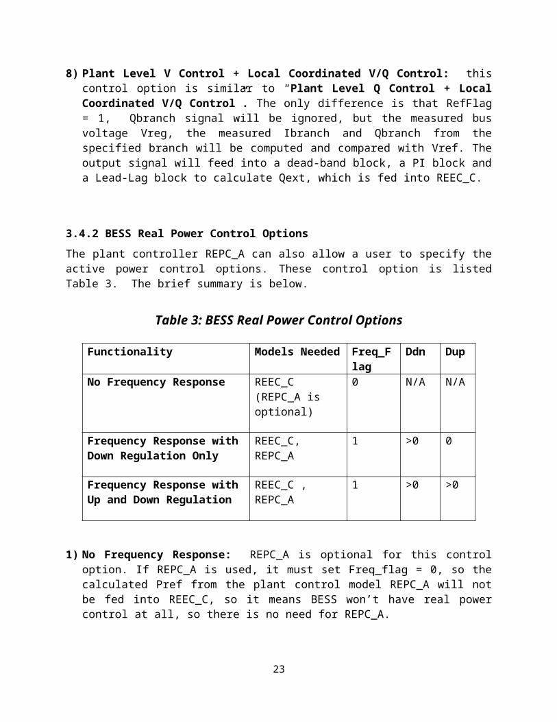
3.4.2 BESS Real Power Control Options

The plant controller REPC_A can also allow a user to specify the active power control options. These control option is listed Table 3. The brief summary is below.

Table 3: BESS Real Power Control Options

Functionality Models Needed Freq_Flag

Ddn Dup

No Frequency Response REEC_C (REPC_A is optional)

0 N/A N/A

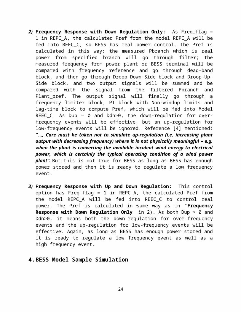
Frequency Response with Down Regulation Only

REEC_C, REPC_A 1 >0 0

Frequency Response with Up and Down Regulation

REEC_C , REPC_A 1 >0 >0

1) No Frequency Response: REPC_A is optional for this control option. If REPC_A is used, it must set Freq_flag = 0, so the calculated Pref from the plant control model REPC_A will not be fed into REEC_C, so it means BESS won’t have real power control at all, so there is no need for REPC_A.

2) Frequency Response with Down Regulation Only: As Freq_flag = 1 in REPC_A, the calculated Pref from the model REPC_A will be fed into REEC_C, so BESS has real power control. The Pref is calculated in this way: the measured Pbranch which is real power from specified branch will go through filter; the measured frequency from power plant or BESS terminal will be compared with frequency reference and go through dead-band block, and then go through Droop-Down-Side block and Droop-Up-Side block, and two output signals will be summed and be compared with the signal from the filtered Pbranch and Plant_pref. The output signal will finally go through a frequency limiter block, PI block with Non-windup limits and lag-time block to compute Pref, which will be fed into Model REEC_C. As Dup = 0 and Ddn>0, the down-regulation for over-frequency events will be effective, but an up-regulation for low-frequency events will be ignored. Reference [4] mentioned: “…, Care must be taken not to simulate up-regulation (i.e. increasing plant output with decreasing

17

frequency) where it is not physically meaningful – e.g. when the plant is converting the available incident wind energy to electrical power, which is certainly the typical operating condition of a wind power plant”. But this is not true for BESS as long as BESS has enough power stored and then it is ready to regulate a low frequency event.

3) Frequency Response with Up and Down Regulation: This control option has Freq_flag = 1 in REPC_A, the calculated Pref from the model REPC_A will be fed into REEC_C to control real power. The Pref is calculated in same way as in “Frequency Response with Down Regulation Only” in 2). As both Dup > 0 and Ddn>0, it means both the down-regulation for over-frequency events and the up-regulation for low-frequency events will be effective. Again, as long as BESS has enough power stored and it is ready to regulate a low frequency event as well as a high frequency event.

4. BESS Model Sample Simulation

As we mentioned in Section 1 Introduction: “at the time of this guideline writing, there is no field test data available for us to validate this newly developed BESS model, so REMTF is looking to BESS manufacturers and power utility companies for the possible test data, so that the future validation simulations and an update of BESS model could be possible”. This section is not a validation simulation to verify this BESS model’s accuracy, but a sample simulation to demonstrate several BESS’s reactive and real power control capabilities. The goal is to get users familiar with BESS models and its control functionalities.

4.1 BESS Generic Model Frequency Response

One of important applications of BESS is to quickly provide backup power when an outage occurs. It might be related to generator drop or load increase in a short time. Whenever the power unbalance happens BESS could be an advantage to regulate frequency and quickly provide backup power. As indicated in Section 2, frequency support is provided by or absorbing real power, being part of AGC or secondary frequency response, is a big advantage BESS has. Federal Energy Regulatory Commission (FERC) Order 755 requires that ISOs implement mechanisms to pay for regulation resources based on how responsive they are to control signals. Under the new rules, storage resources with high-speed ramping capabilities receive greater financial compensation than slower storage or conventional resources.

There are many scenarios where BESS is used to balance power intermittency in power markets. But this section will only look at how BESS can be set up to regulate frequency for the generator drop scenario and load drop scenario. The other scenarios should have similar settings for BESS in order to regulate frequency. The following is regarding the sample case used in this demo, the associated devices and models:

1) The simulation case used is WECC 9-bus-3-Generator, but with BESS replacement of generator on Bus 3. And also additional 20MW generator was set up on Bus 2 to simulate

18

the generator drop scenario. This WECC 9-bus test case represents a simple approximation of the Western Electricity Coordinating Council (WECC) to an equivalent system with nine buses and three generators [6]. The case configuration is shown:

Figure 9: WSCC 9-Bus Test Case with 3 Generators

2) The BESS dynamic models used in this case came from an actual BESS manufacturer with some changes including total capacity being scaled up from 2.2 MWs to 20 MWs, and the original models provided by BESS manufacturer have no REPC_A model, so REPC_A model is added with typical parameters used. The original models provided by BESS manufacturer include the model lhfrt (Low/High frequency ride-through generator protection) and the model lhvrt (Low/High voltage ride-through generator protection). No change is made on these two models. Due to the confidentiality concern, the model data are not be posted here.

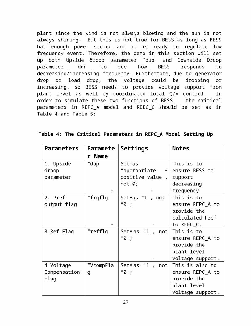
3) As mentioned in Section 3.4.2’s 2), Document [4] doesn’t recommend using this model to simulate the up-regulation function where it is not physically meaningful since the up-regulation function increases plant output with decreasing frequency. This could be an issue for a wind or solar power plant since the wind is not always blowing and the sun is not always shining. But this is not true for BESS as long as BESS has enough power stored and it is ready to regulate low frequency event. Therefore, the demo in this section will set up both Upside Droop parameter “dup” and Downside Droop parameter “ddn” to see how BESS responds to decreasing/increasing frequency. Furthermore, due to generator drop or load drop, the voltage could be dropping or increasing, so BESS needs to provide voltage

19

support from plant level as well by coordinated local Q/V control. In order to simulate these two functions of BESS, the critical parameters in REPC_A model and REEC_C should be set as in Table 4 and Table 5:

Table 4: The Critical Parameters in REPC_A Model Setting Up

Parameters Parameter Name

Settings Notes

1. Upside droop parameter

“dup” Set as “appropriate positive value”, not 0;

This is to ensure BESS to support decreasing frequency

2. Pref output flag “frqflg” Set as “1”, not “0”; This is to ensure REPC_A to provide the calculated Pref to REEC_C.

3 Ref Flag “refflg” Set as “1”, not “0”; This is to ensure REPC_A to provide the plant level voltage support.

4 Voltage Compensation Flag

“VcompFlag” Set as “1”, not “0”; This is also to ensure REPC_A to provide the plant level voltage support.

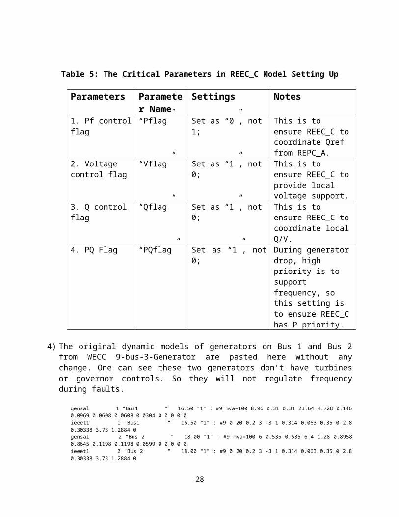
Table 5: The Critical Parameters in REEC_C Model Setting Up

Parameters Parameter Name

Settings Notes

1. Pf control flag “Pflag” Set as “0”, not 1; This is to ensure REEC_C to coordinate Qref from REPC_A.

2. Voltage control flag

“Vflag” Set as “1”, not 0; This is to ensure REEC_C to provide local voltage support.

3. Q control flag “Qflag” Set as “1”, not 0; This is to ensure REEC_C to coordinate local Q/V.

4. PQ Flag “PQflag” Set as “1”, not 0; During generator drop, high priority is to support frequency, so this setting is to ensure REEC_C has P priority.

20

4) The original dynamic models of generators on Bus 1 and Bus 2 from WECC 9-bus-3-Generator are pasted here without any change. One can see these two generators don’t have turbines or governor controls. So they will not regulate frequency during faults.

gensal 1 "Bus1 " 16.50 "1" : #9 mva=100 8.96 0.31 0.31 23.64 4.728 0.146 0.0969 0.0608 0.0608 0.0304 0 0 0 0 0ieeet1 1 "Bus1 " 16.50 "1" : #9 0 20 0.2 3 -3 1 0.314 0.063 0.35 0 2.8 0.30338 3.73 1.2884 0gensal 2 "Bus 2 " 18.00 "1" : #9 mva=100 6 0.535 0.535 6.4 1.28 0.8958 0.8645 0.1198 0.1198 0.0599 0 0 0 0 0ieeet1 2 "Bus 2 " 18.00 "1" : #9 0 20 0.2 3 -3 1 0.314 0.063 0.35 0 2.8 0.30338 3.73 1.2884 0

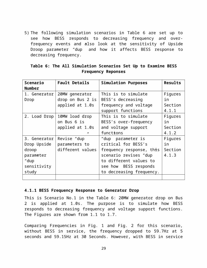
5) The following simulation scenarios in Table 6 are set up to see how BESS responds to decreasing frequency and over-frequency events and also look at the sensitivity of Upside Droop parameter “dup” and how it affects BESS response to decreasing frequency.

Table 6: The All Simulation Scenarios Set Up to Examine BESS Frequency Reponses

Scenario Number Fault Details Simulation Purposes Results1. Generator Drop

20MW generator drop on Bus 2 is applied at 1.0s

This is to simulate BESS’s decreasing frequency and voltage support functions

Figures in Section 4.1.1

2. Load Drop 10MW load drop on Bus 6 is applied at 1.0s

This is to simulate BESS’s over-frequency and voltage support functions


3. Generator Drop Upside droop parameter “dup” sensitivity study

Revise “dup” parameters to different values

“dup” parameter is critical for BESS’s frequency response, this scenario revises “dup” to different values to see how BESS responds to decreasing frequency.


4.1.1 BESS Frequency Response to Generator Drop

This is Scenario No.1 in the Table 6: 20MW generator drop on Bus 2 is applied at 1.0s. The purpose is to simulate how BESS responds to decreasing frequency and voltage support functions. The Figures are shown from 1.1 to 1.7.

Comparing Frequencies in Fig. 1 and Fig. 2 for this scenario, without BESS in service, the frequency dropped to 59.7Hz at 5 seconds and 59.15Hz at 30 Seconds. However, with BESS in service and Upside Droop parameter “dup”=1000 pu/pu settings, the frequency only dropped to 59.85Hz at 5 seconds and starts to increase up to 59.99Hz and stabilized at 59.97Hz at 30 Seconds. Therefore BESS tremendously helps frequency recover for this particular simulation case. For this Scenario, Upside Droop parameter “dup” is set as 1000 pu/pu. This parameter must be appropriately set up, otherwise BESS would not be enough to support frequency recovery or over-respond to frequency’s decrease. The sensitivity study for “dup” is in Scenario No.3. But for different case or scenario, this parameter could be tremendously different.

21

The reason this Scenario set “dup” as 1000 pu is from our initial estimate how much ΔMW/(ΔHz/s) is needed from BESS to recover frequency. As we know “dup” represents the required MW change per frequency change in second, it is basically the slope of ΔMW-ΔFrequency in pu/(pu/s). Figure 1.1 shows that without BESS, frequency dropped from 60Hz to 59.45Hz in 9s(10s-1s), so dup should be

dup= ∆MW∆Hz /∆t

= 20MW(60Hz−59.45Hz)/9 s

= 20MW0.55Hz/9 s

But “dup” must be in per unit whose MW base is BESS Rating 20MW and frequency base is 60Hz, so above equation became

dup= 20MW0.55Hz

=20MW /20MW

( 0.55Hz60Hz

)/9 s= 1

1.0185e-3=981.82 pu

pus

≈1000 pu /( pus

)

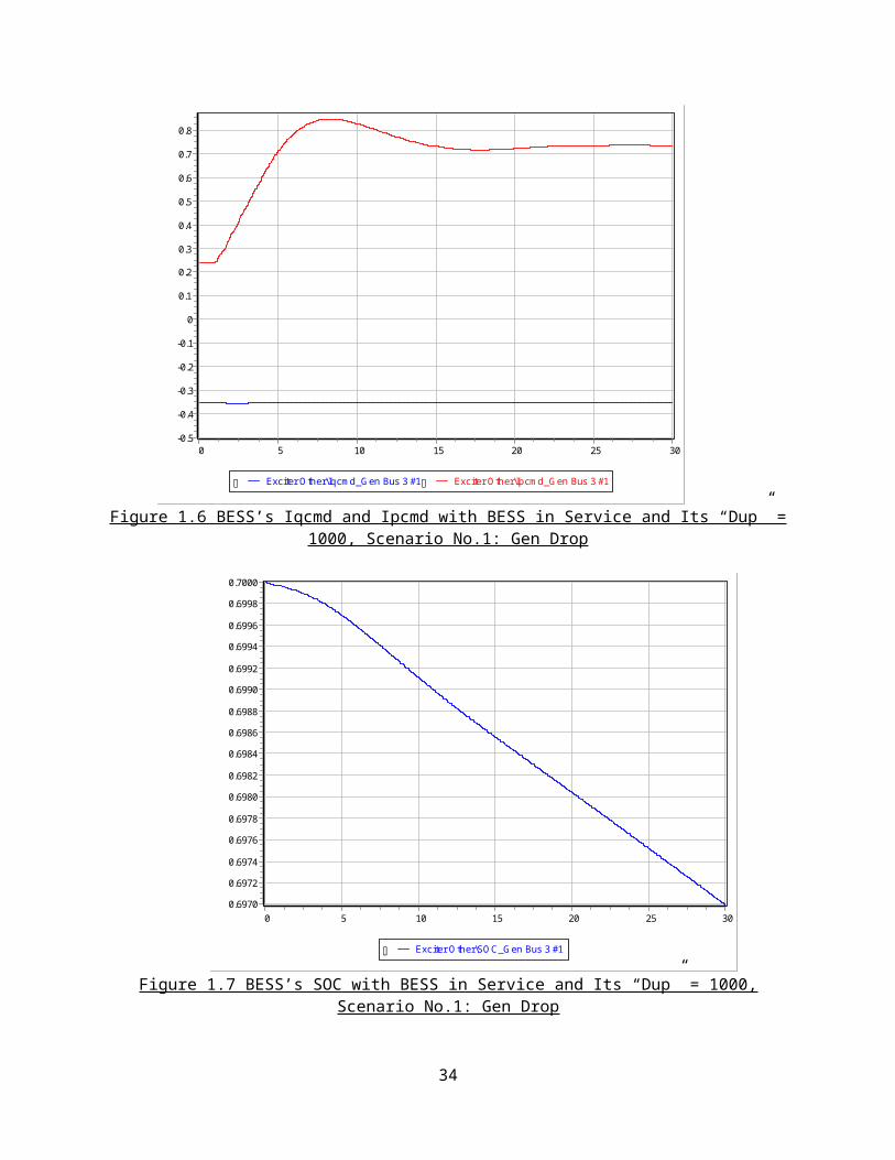
This is why this Scenario set “dup” as 1000 pu. The outputs of BESS’s MW and Ipcmd show real power quickly responds to help frequency recover. But the outputs of BESS’s MVar and Iqcomd don’t increase too much due to P high priority, not Q high priority set up in REEC_C to support frequency recover. If the high priority is Q, MVar and Iqcomd of BESS will increase more. The SOC output shows decreases due to BESS’s comsumption to provide power support.

302520151050

60

59.95

59.9

59.85

59.8

59.75

59.7

59.65

59.6

59.55

59.5

59.45

59.4

59.35

59.3

59.25

59.2

59.15

Frequency_Bus Bus 3gfedcb Frequency_Bus Bus 2gfedcb

Figure 1.1 System Frequency with no BESS, Scenario No.1: Gen Drop

22

302520151050

60

59.99

59.98

59.97

59.96

59.95

59.94

59.93

59.92

59.91

59.9

59.89

59.88

59.87

59.86

59.85


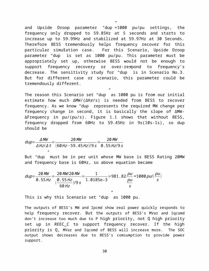
Figure 1.2 System Frequency with BESS and Its “Dup” = 1000, Scenario No.1: Gen Drop

302520151050

1716.5

1615.5

1514.5

1413.5

1312.5

1211.5

1110.5

109.5

98.5

87.5

76.5

65.5

5

MW_Gen Bus 3 #1gfedcb

Figure 1.3 BESS’s MW Output with BESS in Service and Its “Dup” = 1000, Scenario No.1: Gen Drop

23

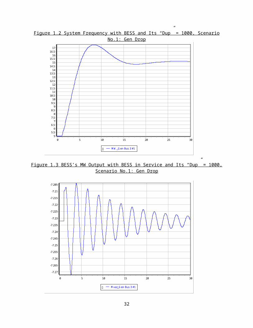
302520151050

-7.205

-7.21

-7.215

-7.22

-7.225

-7.23

-7.235

-7.24

-7.245

-7.25

-7.255

-7.26

-7.265

-7.27

Mvar_Gen Bus 3 #1gfedcb

Figure 1.4 BESS’s MVar Output with BESS in Service and Its “Dup” = 1000, Scenario No.1: Gen Drop

302520151050

1.0280

1.0275

1.0270

1.0265

1.0260

1.0255

1.0250

1.0245

1.0240

1.0235

1.0230

1.0225

1.0220

1.0215

1.0210

1.0205

V pu_Bus Bus 7gfedcb V pu_Bus Bus 3gfedcb

Figure 1.5 Bus Voltages with BESS in Service and Its “Dup” = 1000, Scenario No.1: Gen Drop

24

302520151050

0.8

0.7

0.6

0.5

0.4

0.3

0.2

0.1

0

-0.1

-0.2

-0.3

-0.4

-0.5

Exciter Other\Iqcmd_Gen Bus 3 #1gfedcb Exciter Other\Ipcmd_Gen Bus 3 #1gfedcb

Figure 1.6 BESS’s Iqcmd and Ipcmd with BESS in Service and Its “Dup” = 1000, Scenario No.1: Gen Drop

302520151050

0.7000

0.6998

0.6996

0.6994

0.6992

0.6990

0.6988

0.6986

0.6984

0.6982

0.6980

0.6978

0.6976

0.6974

0.6972

0.6970

Exciter Other\SOC_Gen Bus 3 #1gfedcb

Figure 1.7 BESS’s SOC with BESS in Service and Its “Dup” = 1000, Scenario No.1: Gen Drop

25

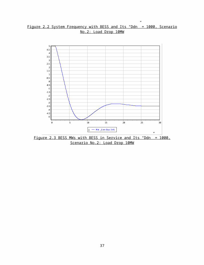
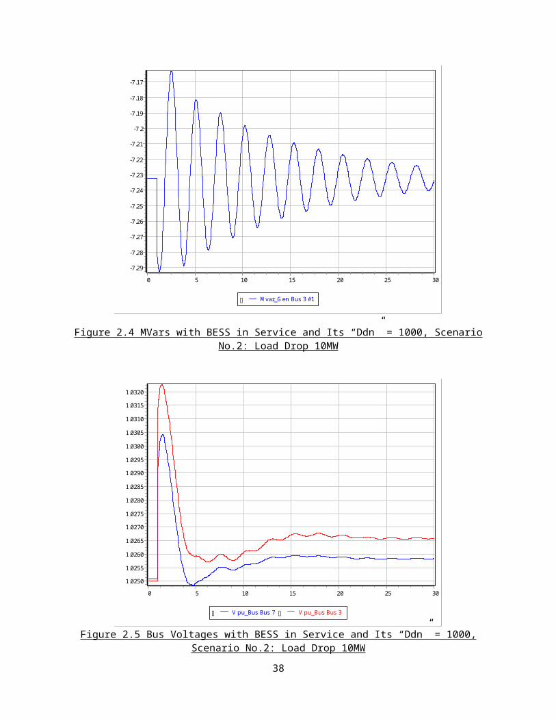
4.1.2 BESS Frequency Response to Load Drop

This is Scenario No.2 in the Table 6: 10MW load drop on Bus 6 is applied at 1.0s. The purpose is to simulate how BESS responds to over-frequency and voltage support functions.

Fig. 2.1 and Fig. 2.2 show that, during 10MW load drop and without BESS in service, the frequency increased to 60.25Hz at 5 seconds and 60.7Hz at 30 Seconds. However, with BESS in service and Downside Droop parameter “ddn”=1000 pu settings, the frequency only increased to 60.13Hz at 5 seconds and starts to decrease and stabilized at 60.02Hz at 30 Seconds. Therefore BESS helps frequency recover for this particular simulation case. For this Scenario and case, Downside Droop parameter “ddn” is set as 1000 pu. This parameter must be appropriately set up, otherwise BESS would not be enough to support frequency recovery. But for different case and scenario, this parameter could be tremendously different.

BESS’s MW and Ipcmd show real power continue to drop and even absort real power to help frequency recover. Same like in Scenario 1: the outputs of BESS’s MVar and Iqcomd don’t increase too much due to P high priority set up in REEC_C to support frequency recovery. The SOC output shows decreases first during P drop and P is till positve in discharging mode, and later increases when P is negative in charging mode.

302520151050

60.7

60.65

60.6

60.55

60.5

60.45

60.4

60.35

60.3

60.25

60.2

60.15

60.1

60.05

60


Figure 2.1 System Frequency with no BESS, Scenario No.2: Load Drop 10MW

26

302520151050

60.12

60.11

60.1

60.09

60.08

60.07

60.06

60.05

60.04

60.03

60.02

60.01

60


Figure 2.2 System Frequency with BESS and Its “Ddn” = 1000, Scenario No.2: Load Drop 10MW

302520151050

5

4.54

3.5

32.5

21.5

1

0.50

-0.5-1

-1.5

-2-2.5

-3-3.5

-4

-4.5-5


Figure 2.3 BESS MWs with BESS in Service and Its “Ddn” = 1000, Scenario No.2: Load Drop 10MW

27

302520151050

-7.17

-7.18

-7.19

-7.2

-7.21

-7.22

-7.23

-7.24

-7.25

-7.26

-7.27

-7.28

-7.29

Mvar_Gen Bus 3 #1gfedcb

Figure 2.4 MVars with BESS in Service and Its “Ddn” = 1000, Scenario No.2: Load Drop 10MW

302520151050

1.0320

1.0315

1.0310

1.0305

1.0300

1.0295

1.0290

1.0285

1.0280

1.0275

1.0270

1.0265

1.0260

1.0255

1.0250

V pu_Bus Bus 7gfedcb V pu_Bus Bus 3gfedcb

Figure 2.5 Bus Voltages with BESS in Service and Its “Ddn” = 1000, Scenario No.2: Load Drop 10MW

28

302520151050

0.8

0.7

0.6

0.5

0.4

0.3

0.2

0.1

0

-0.1

-0.2

-0.3

-0.4

-0.5

Exciter Other\Iqcmd_Gen Bus 3 #1gfedcb Exciter Other\Ipcmd_Gen Bus 3 #1gfedcb

Figure 2.6 Ipcmd and Iqcmd with BESS in Service and Its “Ddn” = 1000, Scenario No.2: Load Drop 10MW

302520151050

0.70055

0.70050

0.70045

0.70040

0.70035

0.70030

0.70025

0.70020

0.70015

0.70010

0.70005

0.70000

0.69995

Exciter Other\SOC_Gen Bus 3 #1gfedcb

Figure 2.7 BESS’s SOC with BESS in Service and Its “Ddn” = 1000, Scenario No.2: Load Drop 10MW

29

4.1.3 BESS Frequency Response Sensitivity on Upside Droop Parameter “ddn” Setting

As we know, both “ddn” and “dup” parameters are critical for BESS’s frequency response. The inappropriate settings for these two parameters might make BESS not capable enough to regulate frequency. And also, for different case and scenario, these two parameters could be tremendously different, so these two parameters must be closely examined to ensure BESS appropriately regulates frequency. But this section only looks at the impact of Upside Droop Parameter “dup” Settings on BESS frequency regulating capabilities. The similar sensitivity study could be used to examine Downside Droop parameter “ddn”.

Table 7 shows 4 different parameters “dup” used to examine BESS’s frequency regulating difference. The fault scenario is same as Scenario No.1 in the Table 5: 20MW generator drop on Bus 2 is applied at 1.0s.

Table 7: The Different Parameters “dup”

Parameter “dup” Settings

Case/Fault Details Results

“dup” = 100 (1). The simulation case is same as in Table 5;

(2). 20MW generator drop on Bus 2 is applied at 1.0s;

Figure 3.1, 3.2

“dup” = 500 Figure 3.3, 3.4

“dup” = 1000 Figure 3.5, 3.6

“dup” = 2000 Figure 3.7, 3.8

The figures from 3.1 to 3.8 show how the Upside Droop Parameter “dup” Settings impact the BESS frequency regulating capabilities. As “dup” Settings increase from 100, 500, 1000 and 2000, BESS frequency response tends to be faster to regulate and stabilize frequency into an acceptable level:

Figure 3.1 shows, when “dup” = 100, the frequency dropped to 59.56Hz at 13 seconds and BESS fails to recover frequency to around 60Hz in 30 seconds, but 59.74hz.

Figure 3.3 shows, with “dup” = 500, BESS’s performance is better, the frequency dropped to 59.78Hz at 6 seconds and BESS recovered frequency to 59.94Hz in 30 seconds, but still not enough.

Figure 3.5 shows, with “dup” = 1000, the frequency only dropped to 59.85Hz at 5 seconds and BESS recovered frequency to 59.97Hz in 30 seconds, which is acceptable, but not the best.

Figure 3.7 shows, with “dup” = 2000, the frequency only dropped to 59.905Hz at 4 seconds and BESS recovered frequency to 59.985Hz in 30 seconds, which is acceptable and best.

30

Once again, for different case and scenario, both “ddn” and “dup” parameters could be tremendously different. In order to ensure BESS appropriately regulates frequency, these two parameters must be closely examined. For this particular simulation case: WSCC 9-bus-3-Generator we used in this demo, the two generators don’t have turbines or governor controls, so these two generators don’t participate in frequency control. In the real world such as a WECC case, lots of generators have turbines modeled, governor controls and even AGC, certainly these generators will coordinate with each other and BESS to control frequency. The detailed simulations should be conducted to figure out both “ddn” and “dup” parameters for BESS.

302520151050

6059.9859.9659.9459.9259.9

59.8859.8659.8459.8259.8

59.7859.7659.7459.7259.7

59.6859.6659.6459.6259.6

59.5859.56


Figure 3.1 System frequency With BESS’s “Dup” = 100, Scenario No.1: Gen Drop 20MW

31

302520151050

13

12.5

12

11.5

11

10.5

10

9.5

9

8.5

8

7.5

7

6.5

6

5.5

5


Figure 3.2 BESS’s MW With BESS’s “Dup” = 100, Scenario No.1: Gen Drop 20MW

302520151050

6059.9959.9859.9759.9659.9559.9459.9359.9259.9159.9

59.8959.8859.8759.8659.8559.8459.8359.8259.8159.8

59.7959.78



32

302520151050

16.516

15.515

14.514

13.513

12.512

11.511

10.510

9.59

8.58

7.57

6.56

5.55



302520151050

60

59.99

59.98

59.97

59.96

59.95

59.94

59.93

59.92

59.91

59.9

59.89

59.88

59.87

59.86

59.85



33

302520151050

1716.5

1615.5

1514.5

1413.5

1312.5

1211.5

1110.5

109.5

98.5

87.5

76.5

65.5

5



302520151050

60

59.995

59.99

59.985

59.98

59.975

59.97

59.965

59.96

59.955

59.95

59.945

59.94

59.935

59.93

59.925

59.92

59.915

59.91

59.905



34

302520151050

17

16

15

14

13

12

11

10

9

8

7

6

5



4.2 BESS Voltage and Reactive Power Control Response

Although BESS’s voltage and reactive power control are not the primary use, they are occasionally used as auxiliary service. When BESS is used for this purpose it works just like a regular Type-3 or Type-4 wind generator or solar power plant. So these types of simulations are almost the same. Therefore, this document will not simulate these functions. For the detailed simulation, users can look at Reference [4, 5].

When simulating BESS’s voltage and reactive power control, just like simulating Type-3 or Type-4 wind generators or solar power plants, users must pay attention to the parameters of PfFlag, Vflag, Qflag and RefFlag, to ensure their settings to follow Table 1 based on their specific control situation. And also, PQflag usually should be set as Q priority to ensure BESS has effective voltage and reactive power control.

5. References

[1]. Puget Sound Energy, “Electrical Energy Storage Assessment”, 2015.

[2]. WECC Modeling and Validation Working Group, “Value and Limitations of the Positive Sequence Generic Models of Renewable Energy Systems”.

35

[3]. WECC Modeling and Validation Work Group. WECC Renewable Energy Modeling Task Force Report. (2015, Mar.). Adhoc Group on BESS Modeling. WECC energy storage system model - Phase II. Salt Lake City, UT. [Online]. Available:https://www.wecc.biz/Reliability/WECC%20Approved%20Energy%20Storage%20System%20Model%20-%20Phase%20II.pdf orP. Pourbeik, “Simple Model Specification for Battery Energy Storage System”, Prepared by EPRI, Rev 3. 3/18/15. Issued to WECC REMTF and EPRI P173.003

[4]. WECC Modeling and Validation Working Group, “WECC Type 4 Wind Turbine Generator Model – Phase II” January 23, 2013.

[5]. WECC Modeling and Validation Working Group, “WECC Solar Plant Dynamic Modeling Guidelines” May 8, 2014.

[6]. Illinois Center for a Smarter Electric Grid, http://icseg.iti.illinois.edu/wscc-9-bus-system/

[7]. PowerWorld Model Manual, http://www.powerworld.com/WebHelp/Default.htm#cshid=TSModels_Exciter_REEC_C

[8]. P. Pourbeik, S. E. Williams, J. Weber,J. Sanchez-Gasca, J. Senthil, S. Huang and K. Bolton, "Modeling and Dynamic Behavior of Battery Energy Storage", IEEE Electrification Magazine, September 2015.

[9]. WECC Second Generation Wind Turbine Models, January 23, 2014. https://www.wecc.biz/Reliability/WECC-Second-Generation-Wind-Turbine-Models-012314.pdf

[10]. X. Xu, M. Bishop, D. G. Oikarinen and C. Hao, "Application and Modeling of Battery Energy Storage in Power Systems," CSEE Journal of Power and Energy Systems, Vol. 2, No. 3, September 2016, pp.82-90 [Online]. Available in IEEE Xplore Digital Library:http://ieeexplore.ieee.org/stamp/stamp.jsp?arnumber=7562828

[11]. X. Xu, E. Casale, M. Bishop, and D.G. Oikarinen, “Application of New Generic Models for PV and Battery Storage in System Planning Studies,” in Proc. IEEE Power Energy Soc. Gen. Meeting, Chicago, IL, USA, Jul. 2017.

36

http://ieeexplore.ieee.org/stamp/stamp.jsp?arnumber=7562828

https://www.wecc.biz/Reliability/WECC-Second-Generation-Wind-Turbine-Models-012314.pdf

https://www.wecc.biz/Reliability/WECC-Second-Generation-Wind-Turbine-Models-012314.pdf

http://www.powerworld.com/WebHelp/Default.htm#cshid=TSModels_Exciter_REEC_C

http://icseg.iti.illinois.edu/wscc-9-bus-system/

https://www.wecc.biz/Reliability/WECC%20Approved%20Energy%20Storage%20System%20Model%20-%20Phase%20II.pdf

https://www.wecc.biz/Reliability/WECC%20Approved%20Energy%20Storage%20System%20Model%20-%20Phase%20II.pdf

APPENIDX

A. Parameters for REEC_C Model

The WECC document “WECC Type 4 Wind Turbine Generator Model – Phase II”[4] provides the details of parameter information for Model REPC_A, REEC_A and REGC_A. Those parameter information can same apply to Model REPC_A, a part of REEC_C and REGC_A used in this guideline. As REEC_C is the augmented version of REEC_A, only 4 additional parameters T, SOCini, SOCmin and SOCmax need to add to the original REEC_A parameter sets. So, this document will only provide info for these 4 parameters. User can go to The WECC document “WECC Type 4 Wind Turbine Generator Model – Phase II”[4] to check other parameters.

Parameter Description Typical Range of Values

Units

T BESS rated Charging or Discharging time

3600s ~ 36000s (1 hour to 10 hours, consulting BESS vendor)

seconds

SOCini The initial State of Charge 20% ~ 80% %, percentageSOCmin The minimal State of Charge

BESS can discharging down to or should be kept on

10% ~ 20% %, percentage

SOCmax The maximum State of Charge BESS can charging up to

75% ~ 85% %, percentage

38

wecc battery storage guideline - western electricity ... battery storage... · web viewwecc battery...

Documents