REPEATED COOPERATION WITH OUTSIDE OPTIONS

BY TAKAKO FUJIWARA-GREVE AND YOSUKE YASUDA1

Keio University; National Graduate Institute of Policy Studies (GRIPS), JAPAN.

If agents can choose when to end a repeatable interaction as well as what to do within the part-nership, cooperation incentives are interrelated with the ending decision. Using a Prisoner’s Dilemmawith outside options, we investigate how the structure of outside options affects the ease of cooperation,measured by the minimum discount factor that sustains mutual cooperation. One-sided outside op-tions do not make cooperation easier than ordinary repeated games, but uncertainty of options reducesthe difficulty by enabling cooperation until a good option realizes. Two-sided and very low outsideoptions make cooperation easier than ordinary repeated games. Economic implications abound.

1. INTRODUCTION

In many economic interactions, whether and how a relationship is continued affect how agents

act within the relationship. An extreme case is the repeated Prisoner’s Dilemma (a moral hazard

problem): if the interaction ends at a known finite period, then all players act myopically, while if the

game is repeated forever, or the last period is uncertain, then a variety of equilibrium behaviors are

possible. These are models with exogenous ending of repeated games and are extensively studied.2

In reality, it is not always plausible that the game’s length is independent of what players do in the

game. It is more natural that players’ in-game performance (payoffs or actions) affects how long the

interaction lasts. We formulate this endogenous ending of repeated interactions by allowing player(s)

to strategically end a repeated Prisoner’s Dilemma by taking an outside option.3 Specifically, the

1The authors are grateful to Bo Chen, Henrich Greve, Ariel Rubinstein, Takashi Shimizu, Satoru Takahashi, andseminar participants at Stony Brook Game Theory Festival (2009), KIER Kyoto University, 11th SAET conference(Portugal, 2011), and AMES (Seoul, 2011) for useful comments. Usual disclaimer applies. Financial support from JSPS,Gant-in-Aid for Scientific Research (C), 21530171 for Fujiwara-Greve and Grant-in-Aid for Young Scientists (Start-up),20830024 for Yasuda is gratefully acknowledged. Please address correspondence to: Takako Fujiwara-Greve, Departmentof Economics, Keio University, 2-15-45 Mita, Minato-ku, Tokyo, 108-8345 JAPAN. E-mail: takakofg@econ.keio.ac.jp.

2For finitely repeated games, see Benoit and Krishna (1985). For infinitely or stochastically repeated games, seeFudenberg and Maskin (1986) and Abreu (1988). For an overview, see Mailath and Samuelson (2006). Exogenous andstochastic ending models are studied by Neyman (1999) and Neyman and Sorin (2010).

3Our model as well as the line of voluntarily repeated games (e.g., Datta, 1996, Ghosh and Ray, 1996, Kranton, 1996a,Fujiwara-Greve and Okuno-Fujiwara, 2009, and McAdams, 2011) are “active” ending models, where players strategicallychoose to end an interaction. There is also a class of “passive” but endogenous ending models such as the ruin gameby Rosenthal and Rubinstein (1984), financial constraint models by Bevia, Corchon and Yasuda (2011) and Kawakami(2010), and R&D model by Furusawa and Kawakami (2008). For a given horizon of a repeated game, Casas-Arce (2010)analyzes how firing and quitting option affects the folk theorem. Watson (1999, 2002) constructs an optimal long-runbehavior when defection terminates the interaction.

1

model is as follows. Two players engage in a repeated Prisoner’s Dilemma. At the end of each period,

an outside option becomes available, which summarizes the future payoff after ending the current

game. The player who has an outside option can either reject it to continue the repeated game with

the current partner or take it to terminate the game. As long as no player takes an outside option,

the game continues. This model is inspired by employment relationships in which a worker is initially

matched with a firm but may receive offers from other firms at intervals. This is a one-sided outside

option case. Another important example of the one-sided option model is repeatable purchase, where

a buyer can repeat transactions with the same seller or switch sellers. In an employment relationship,

if the firm can also replace the current worker with a new one, it becomes a two-sided outside option

model. Other two-sided outside option situations include firm collusion, co-authorships, business

partners, and married couples.

We investigate the relationship between the ease of cooperation and the structure of the outside

options. The ease of cooperation is measured by the minimum discount factor that sustains some

repetition of mutual cooperation as a subgame perfect equilibrium outcome. When players are free to

quit, one might think that cooperation never becomes easier than in the repeated game (commitment

to stay) situation. This intuition is correct for the one-sided outside option case, where punishment

against the player who has outside options cannot be stricter than the one in the repeated game

situation. However, if both players have outside options and can unilaterally end the game, it can be

easier to sustain repeated cooperation than in the repeated game. This is because players can impose

on each other a lower payoff (of an outside option) than those in the game.

Whether the outside options are certain or not also affects the ease of cooperation. In ordinary re-

peated games, payoff fluctuation or discount factor fluctuation has only negative effect on cooperation,

as shown by Rotemberg and Saloner (1986) and Dal Bo (2007). The key to these negative results is

that, when fluctuation creates difficulty for cooperation (a high deviation payoff or a low value of the

discount factor), the players, who are confined in the repeated game, need to reduce the level of co-

operation in that period. This reduces the on-path payoff, i.e., the incentive to follow the equilibrium

strategy. Therefore the players need to be more patient to cooperate under payoff/discount factor

2

fluctuation than in the deterministic case.4 By contrast, if the outside option value fluctuates, players

can selectively take only high options, as opposed to demand shocks or discount factor volatilities that

affect all actions’ payoffs. This “option” structure allows uncertainty to have an effect only when the

value increases, providing more cooperation incentives within the current partnership.

Positive effects of game-parameter volatility on cooperation is a new insight in the literature of

dynamic games.5 However, in the two-sided option case, the positive effect is weakened. This is because

a player may end up with a low option when the partner received a high option and terminates the

game. Thus negative correlation of the outside options across players reduces the cooperation incentive.

Overall, cooperation is easy in “symmetric” partnerships, where both players have outside options and

those are positively correlated.

In summary, we have an extensive study of varying outside option structure to repeated Prisoner’s

Dilemma and show that external payoff structure matters for in-game cooperation incentives. There

are many economic implications that can be addressed within our framework. For example, for the

one-sided outside option model as interpreted as an employment relationship, we predict that workers

with different mean of the distributions of outside options behave differently under economic volatility

which alters the spread of option values. “High-mean” workers effectively become more patient or

cooperative under wider spread of outside options, because they cooperate only until a good option

realizes and this play path yields higher expected future payoff under volatility. By contrast, “low-

mean” workers, who do not intend to take an outside option while cooperating, may consider taking

one if they deviate. In this case, more volatility of outside options increases the value of deviation,

while the value of cooperation is fixed, and workers become less cooperative under economic volatility.

To place our paper in a larger context, there are many related fields. The closest is the literature

of voluntarily repeated games, in which a player can choose to play the same stage game with the

current partner or end the partnership and find a new partner in a random matching process, without

information flow.6 In this literature, although each partnership may end strategically, the ex-ante

4A similar argument is noted in Mailath and Samuelson (2006), pp.176-177.5A similar positive effect of payoff volatility in a repeated game is analyzed in Yasuda and Fujiwara-Greve (2011).6The literature of voluntarily repeated games is very large. Datta (1996), Kranton (1996a), Carmichael and MacLeod

(1997), and Fujiwara-Greve and Okuno-Fujiwara (2009) are complete information models and Ghosh and Ray (1996),

3

equilibrium continuation payoff after a partnership ends is unique, because the no-information-flow

and random matching assumption imply that all new partnerships give the same ex-ante long-run

payoff in an equilibrium. By contrast, our model allows heterogeneous future payoffs after the current

interaction ends.

Search theory, alternating-offer bargaining models, and contract theory also incorporate outside

options. In search theory, outside option structure affects quitting/search behavior but often within-

firm behaviors (work incentives) is not addressed.7 In both bargaining models and our model, outside

option structure matters for equilibrium behavior but in a different way.8 In bargaining, efficiency

is enhanced when parties want to end the game as soon as possible, while in repeated Prisoner’s

Dilemma, efficiency is enhanced when parties want to continue the game while cooperating.

In basic contract theory, outside payoffs are incorporated to determine the minimum payment

and do not affect incentives after a contractual relationship is started. Dynamic, relational contract

models have not consider endogenous ending nor stochastic outside payoffs until recently.9 Wang and

Yang (2011) studied a dynamic hiring model similar to voluntarily repeated games mentioned above,

where the employee has a stochastic outside opportunity each period. However, incentive analysis is

absent in their paper. Our model, although simple, has both explicit dynamic incentive structure and

stochastic participation constraint.

The paper is organized as follows. In Section 2, we give a motivating example to show how different

structures of outside options change the cooperation incentives for mid-range discount factors. In

Section 3, we introduce a one-sided outside option model with a benchmark analysis. Section 4 is the

main analysis of the one-sided outside option model. Section 5 analyzes two-sided outside options,

Kranton (1996b), and Rob and Yang (2010) are incomplete information models. McAdams (2011) analyzes a stochasticgame type model where the stage-game payoff follows a random walk over time. Although not in a dynamic context,Okuno (1981) and Shapiro and Stiglitz (1984) are pioneering works that addressed the relationship between incentivesand the threat of termination of the relationship.

7For example, the classical model by Jovanovic (1979) does not have on-the-job search and a firm-worker matchquality is random and exogenous, which determines the utility within a match. Burdett (1978) allows on-the-job-searchbut no action choice within an employment relationship. Pissarides (1994) considers an on-the-job-search model in whichsearch increases the match surplus, but there is no action choice within a match other than splitting the surplus withthe employer.

8For bargaining models with various outside option structures, see, for example, Ponsatı and Sakovics (1998, 2001)and Compte and Jehiel (2002).

9In relational contract models, uncertainty of outside options tends to mean adverse selection. For example, Halac(2011) analyzed a model in which the principal’s outside option is deterministic but a private information.

4

and Section 6 concludes the paper.

2. MOTIVATING EXAMPLE

Consider two players, Player 1 and 2, who are engaged in the Prisoner’s Dilemma of Table 1, over a

discrete horizon t = 1, 2, . . ..

P1 \ P2 C DC 6, 6 0, 7D 7, 0 2, 2

Table 1: An example

In each period, after the Prisoner’s Dilemma is played, an outside option becomes available to

Player 1. An outside option is a total future payoff for Player 1 after ending the current game. Player

2 has no option to end the game. The game repeats (Prisoner’s Dilemma and then an outside option)

as long as Player 1 does not take an outside option, and each player maximizes the total expected

discounted payoff (for Player 1 this includes the payoff from an outside option) with a discount factor

δ ∈ (0, 1). Suppose that, in any period, the outside option is the same and gives the total payoff of

5.51−δ to Player 1 after exit. Player 2’s payoff after Player 1 ends the game is normalized to be zero.

Let the common discount factor be δ = 0.6. If the game is an ordinary repeated game without the

outside option, infinitely repeated cooperation (C,C), (C,C), . . . (which we call eternal cooperation)

is sustainable by the grim trigger strategy since

61 − δ

= 15 > 7 + δ2

1 − δ= 10.

As the outside option 5.51−δ is available, however, Player 1 can play D and then take the outside

option, making the continuation value 5.51−δ . Therefore, Player 1 does not follow eternal cooperation

(C,C), (C,C), . . . in this case, since

61 − δ

= 15 < 7 + δ5.5

1 − δ= 15.25.

This illustrates that the existence of an outside option greater than the in-game punishment payoff

creates difficulty in achieving cooperation, in the sense that the range of discount factors that sustain

5

repeated cooperation shrinks.

Next, suppose that the outside option is uncertain, such that at the end of each period, either

6.81−δ or 4.2

1−δ is the realized option, with equal probability. Note that the average is still 5.51−δ . We show

that it is possible for Player 1 to cooperate until the good option 6.81−δ realizes. The play path “(C,C),

(C,C), . . ., until Player 1 exits” is called stochastic cooperation.

The logic is as follows. If Player 1 follows the stochastic cooperation, the total expected payoff

can be written as

6 + δV,

where V is the expected continuation payoff of waiting for the good option while cooperating, which

satisfies the following recursive formula.

V =12· 6.81 − δ

+12{6 + δV }.

To explain, at the end of a period, with probability 1/2, the good option realizes and Player 1’s

continuation payoff becomes 6.81−δ . With probability 1/2, the bad option realizes, in which case Player

1 continues the repeated game and the situation is the same as before.

By computation, at δ = 0.6, 6 + δV ≈ 15.86. Therefore, the expected payoff of stochastic cooper-

ation is greater than that of eternal cooperation.

Let us compare with the deviation value. If Player 1 exits immediately after deviation, the total

expected payoff is 7 + δ{(12) 6.8

1−δ + (12) 4.2

1−δ} = 15.25 as before. Player 1 can also wait for the good

option after deviation. In that case her total expected payoff is of the form

7 + δW,

where W satisfies

W =12· 6.81 − δ

+12{2 + δW},

by the same logic as the formulation of V . By computation, 7+δW ≈ 15.14. Therefore, it is optimal to

exit immediately by taking any option, but still the payoff from stochastic cooperation is greater than

the payoff of optimal deviation. Hence although eternal cooperation cannot be sustained at δ = 0.6

6

and a fixed option of 5.51−δ , if the outside options are stochastic, repeated cooperation is sustained until

the good option realizes.

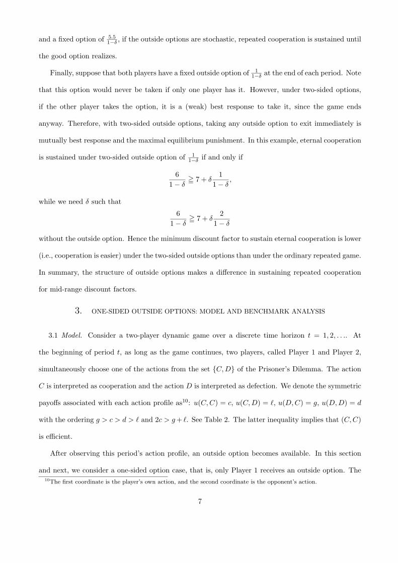
Finally, suppose that both players have a fixed outside option of 11−δ at the end of each period. Note

that this option would never be taken if only one player has it. However, under two-sided options,

if the other player takes the option, it is a (weak) best response to take it, since the game ends

anyway. Therefore, with two-sided outside options, taking any outside option to exit immediately is

mutually best response and the maximal equilibrium punishment. In this example, eternal cooperation

is sustained under two-sided outside option of 11−δ if and only if

61 − δ

= 7 + δ1

1 − δ,

while we need δ such that

61 − δ

= 7 + δ2

1 − δ

without the outside option. Hence the minimum discount factor to sustain eternal cooperation is lower

(i.e., cooperation is easier) under the two-sided outside options than under the ordinary repeated game.

In summary, the structure of outside options makes a difference in sustaining repeated cooperation

for mid-range discount factors.

3. ONE-SIDED OUTSIDE OPTIONS: MODEL AND BENCHMARK ANALYSIS

3.1 Model. Consider a two-player dynamic game over a discrete time horizon t = 1, 2, . . .. At

the beginning of period t, as long as the game continues, two players, called Player 1 and Player 2,

simultaneously choose one of the actions from the set {C,D} of the Prisoner’s Dilemma. The action

C is interpreted as cooperation and the action D is interpreted as defection. We denote the symmetric

payoffs associated with each action profile as10: u(C,C) = c, u(C,D) = `, u(D,C) = g, u(D,D) = d

with the ordering g > c > d > ` and 2c > g + `. See Table 2. The latter inequality implies that (C,C)

is efficient.

After observing this period’s action profile, an outside option becomes available. In this section

and next, we consider a one-sided option case, that is, only Player 1 receives an outside option. The10The first coordinate is the player’s own action, and the second coordinate is the opponent’s action.

7

P1 \ P2 C DC c, c `, g

D g, ` d, d

Table 2: General Prisoner’s Dilemma

game continues to the next period if and only if Player 1 does not take the outside option that arrived

in that period. Each player maximizes the total expected discounted payoff11 with a common discount

factor δ ∈ (0, 1).

The total long-run payoff of an outside option is of the form12 x/(1 − δ) and we identify each

outside option by the average payoff x. In this section, we give the benchmark result when there is

only one option v in any period.

Player 2 receives payoffs only from the Prisoner’s Dilemma and does not have the ability to end

the game, as in the ordinary repeated games. Let us also assume that d = 0 which implies that Player

2’s “outside payoff” 0 is not better than the payoff from (D,D).13 Figure 1 depicts the outline of the

dynamic game.

If Player 1 takes an outside option v at the end of T -th period, her total payoff is

T∑t=1

δt−1u(a1(t), a2(t)) + δT v

1 − δ,

while Player 2’s total payoff isT∑

t=1

δt−1u(a2(t), a1(t)),

where ai(t) is the action of Player i in t-th period of the repeated Prisoner’s Dilemma.

We assume that all actions are observable to the players. Therefore, in period t = 2, players can

base their actions on the history of past action profiles. The game is of complete information. As the

equilibrium concept, we use subgame perfect equilibrium (SPE henceforth).

As we discussed in the introduction, there are many economic situations that fit this model. For

example, we can interpret the model as an employment relationship, in which a worker (Player 1) is

11Alternatively one can assume that the players maximize the average payoffs without changing the qualitative results.12If the outside option is independent from (1 − δ), it becomes irrelevant when δ is sufficiently large.13The qualitative results do not change as long as Player 2’s outside payoff is not greater than Player 1’s outside

option. See Section 5.

8

-Period 1 Period 2 time

¾½

»¼PD -?

outside option

µ´¶³1 -

Not take

QQ

QQQs

Takeoption v

P1: v/(1 − δ)

P2: 0

¾½

»¼PD -?

outside option

µ´¶³1 -

Not take

QQ

QQQs

Takeoption v

P1: v/(1 − δ)

P2: 0

Figure 1: Outline of the one-sided fixed-option game

free to quit but the firm (Player 2) cannot easily fire a worker.14 Another example is a buyer-seller

relationship in which only the buyer can walk away from the seller.15

We investigate the range of δ in which repeated mutual cooperation of (C,C) is sustained as long

as possible, under a variety of structures of the outside options. Although it is an easy extension

to investigate other stationary action profiles on the play path, there are enough reasons to focus

on repeated (C,C). First, when the Prisoner’s Dilemma payoffs satisfy the supermodular condition,

repetition of (C,C) is the easiest stationary action profile to sustain.

REMARK 1. (Stahl, 1991) For any infinitely repeated symmetric Prisoner’s Dilemma such that

u(C,C) + u(D,D) = u(C,D) + u(D,C), the minimum discount factor that sustains repeated (C,C)

on the play path is not greater than the one that sustains (C,D) or (D,C).

Hence, it suffices to consider the repetition of (C,C) to determine the minimum discount factor

that sustains some non-myopic action profile. The example in Section 2 satisfies this condition.

Second, when we consider two-sided outside options (Section 5), an asymmetric action profile such

as (C,D) and (D,C) would be more difficult to sustain, because the player with a lower in-game

payoff requires a higher discount factor to follow the target strategy. Since we cover both one-sided

and two-sided option cases, the symmetric action profile (C,C) gives the clearest comparison.

Third, our interest is how the structure of outside options affects the lower bound of the discount

factors that sustain mutual cooperation, not the absolute value of the lower bound. The comparative

14It may be possible for Player 2 to play actions that give low payoff to Player 1 to induce quit.15See Casas-Arce (2010) for a real-world example of fishing arrangements of this sort.

9

statics results (subsection 4.4) do not depend on the focus on (C,C).

Fourth, the pure action profile (C,C) has a clear meaning in economics, for example, honest

transactions, contribution to public good, and absence of moral hazard. Other action combinations

may not have such clear interpretation.

Therefore, in this paper we focus on repeated (C,C) as long as possible. To determine the minimum

discount factor that establishes a subgame perfect equilibrium, we need to find out the maximal

equilibrium punishment. If the maximal equilibrium punishment does not sustain the on-path action

profile, no other punishment would, by the same logic as the optimal penal code in Abreu (1988).

Therefore, without loss of generality we consider the following class of strategy combinations, which

we call simple trigger strategy combinations.

Cooperation phase: If the history is empty or does not have D, play (C,C) and Player 1’s exit

decision is optimal given that (C,C) is repeated as long as the game continues.

Punishment phase: If the history contains D, play (D,D) and Player 1’s exit decision is optimal

given that (D,D) is repeated as long as the game continues.

Note that Player 1’s optimal exit decision depends not only on the phase (the expected future

play) but also on the structure of outside options. In the following, for each outside option structure,

we derive an optimal exit decision rule given that players follow either (C,C) or (D,D) as long as the

game continues. Then we can completely specify an equilibrium strategy combination.

3.2. Fixed Option Analysis. As the benchmark, we consider the case that the same option v is

available for Player 1 at the end of any period. This gives v/(1 − δ) in total to Player 1 when she

takes it, as depicted in Figure 1. Since the outside option is the same at any period, the optimal exit

decision rule for Player 1 is either to take the option as soon as possible or never to take it.

If v 5 d, then the optimal exit rule for Player 1 is not to take the outside option v in any phase, thus

the game is effectively the ordinary repeated Prisoner’s Dilemma. In this case, eternal cooperation is

sustained by the simple trigger strategy combination if and only if

c

1 − δ= g +

δd

1 − δ⇐⇒ δ = g − c

g − d=: δ.

10

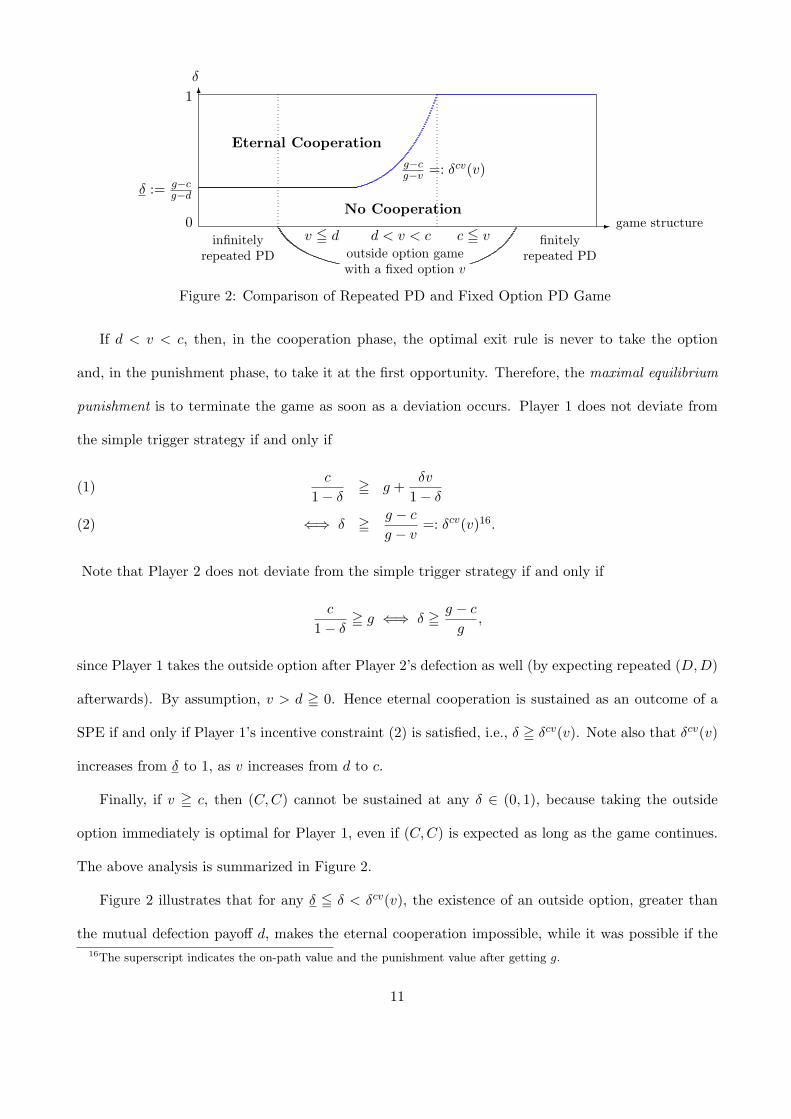
- game structure

6

δ := g−cg−d

No Cooperation

Eternal Cooperationg−cg−v =: δcv(v)

0

1δ

infinitelyrepeated PD

v 5 d d < v < c c 5 voutside option gamewith a fixed option v

finitelyrepeated PD

Figure 2: Comparison of Repeated PD and Fixed Option PD Game

If d < v < c, then, in the cooperation phase, the optimal exit rule is never to take the option

and, in the punishment phase, to take it at the first opportunity. Therefore, the maximal equilibrium

punishment is to terminate the game as soon as a deviation occurs. Player 1 does not deviate from

the simple trigger strategy if and only if

c

1 − δ= g +

δv

1 − δ(1)

⇐⇒ δ = g − c

g − v=: δcv(v)16.(2)

Note that Player 2 does not deviate from the simple trigger strategy if and only if

c

1 − δ= g ⇐⇒ δ = g − c

g,

since Player 1 takes the outside option after Player 2’s defection as well (by expecting repeated (D,D)

afterwards). By assumption, v > d = 0. Hence eternal cooperation is sustained as an outcome of a

SPE if and only if Player 1’s incentive constraint (2) is satisfied, i.e., δ = δcv(v). Note also that δcv(v)

increases from δ to 1, as v increases from d to c.

Finally, if v = c, then (C,C) cannot be sustained at any δ ∈ (0, 1), because taking the outside

option immediately is optimal for Player 1, even if (C,C) is expected as long as the game continues.

The above analysis is summarized in Figure 2.

Figure 2 illustrates that for any δ 5 δ < δcv(v), the existence of an outside option, greater than

the mutual defection payoff d, makes the eternal cooperation impossible, while it was possible if the16The superscript indicates the on-path value and the punishment value after getting g.

11

game were an ordinary repeated Prisoner’s Dilemma. Therefore, the existence of a fixed one-sided

outside option does not make repeated cooperation easier than in ordinary repeated games.

Next, we show that when the outside option becomes uncertain, this difficulty can be reduced.

4. ONE-SIDED OUTSIDE OPTIONS: STOCHASTIC OPTIONS

4.1. Binary Option Model. In many economic situations, it is more plausible that the outside options

are not certain. For example, workers may not know the exact value of an offer from a potential

employer until it arrives. In this section we consider a simple model of binary i.i.d. distributions of

outside options, and maintain the complete information assumption; players know the distribution of

outside options. (In subsection 4.5, we discuss how the main results extend to models of more than

two options.) The randomness of outside options can be interpreted several ways, such as external

perturbation or a draw from a distribution of options.

The uncertainty of the options allows stochastic cooperation (cooperation until some stochastic op-

tion arrives) as the play path of a simple trigger strategy combination, in addition to eternal coopera-

tion and no cooperation. It is then possible that the volatility of outside options enhances cooperation

by changing the on-path play from no cooperation to stochastic cooperation, as we illustrated by the

motivating example.

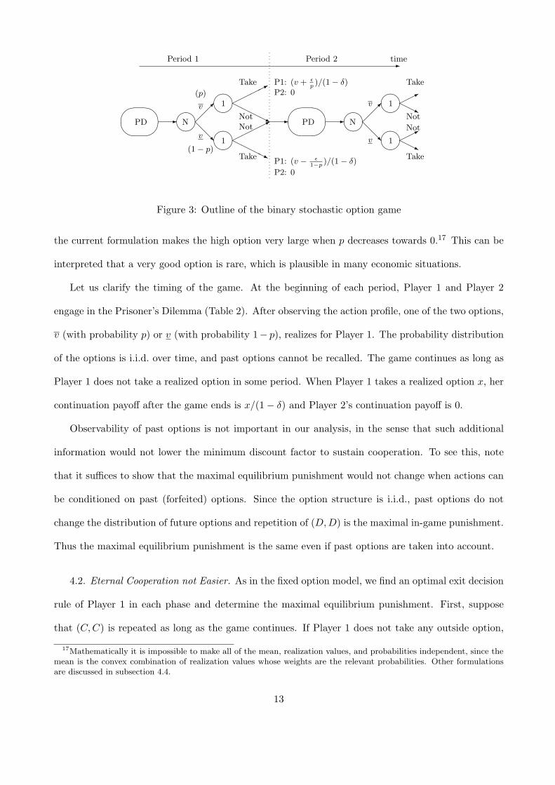
To compare with the fixed option model, let v be the mean of stochastic options and independent

from their spread and probabilities. Specifically, we focus on distributions such that a high option,

which gives (v + εp)/(1 − δ) in total, arrives with probability p and a low option, which gives (v −

ε1−p)/(1 − δ) in total, arrives with probability (1 − p), for some ε > 0. (See Figure 3.) This way, the

mean of the two options is v/(1 − δ) for any p ∈ (0, 1) and any ε > 0. The spread between the two

options is proportional to ε;

11 − δ

{(v +ε

p) − (v − ε

1 − p)} =

1p(1 − p)(1 − δ)

ε.

Hence increasing ε corresponds to the mean-preserving spread. We identify the two options by the

average payoff, v := v + εp and v := v − ε

1−p . Note that change in p affects the values of options, and

12

-Period 1 Period 2 time

¾½

»¼PD -µ´¶³

N ¡¡µ

(p)

v

@@Rv

(1 − p)

µ´¶³1 ©©©©*

HHHHj

Take

Not

µ´¶³1 ©©©©*

HHHHj

Not

Take

P1: (v + εp)/(1 − δ)

P2: 0

P1: (v − ε1−p

)/(1 − δ)

P2: 0

-

¾½

»¼PD -µ´¶³

N ¡¡µ

v

@@Rv

µ´¶³1 ©©*

HHj

Take

Not

µ´¶³1 ©©*

HHj

Not

Take

Figure 3: Outline of the binary stochastic option game

the current formulation makes the high option very large when p decreases towards 0.17 This can be

interpreted that a very good option is rare, which is plausible in many economic situations.

Let us clarify the timing of the game. At the beginning of each period, Player 1 and Player 2

engage in the Prisoner’s Dilemma (Table 2). After observing the action profile, one of the two options,

v (with probability p) or v (with probability 1− p), realizes for Player 1. The probability distribution

of the options is i.i.d. over time, and past options cannot be recalled. The game continues as long as

Player 1 does not take a realized option in some period. When Player 1 takes a realized option x, her

continuation payoff after the game ends is x/(1 − δ) and Player 2’s continuation payoff is 0.

Observability of past options is not important in our analysis, in the sense that such additional

information would not lower the minimum discount factor to sustain cooperation. To see this, note

that it suffices to show that the maximal equilibrium punishment would not change when actions can

be conditioned on past (forfeited) options. Since the option structure is i.i.d., past options do not

change the distribution of future options and repetition of (D,D) is the maximal in-game punishment.

Thus the maximal equilibrium punishment is the same even if past options are taken into account.

4.2. Eternal Cooperation not Easier. As in the fixed option model, we find an optimal exit decision

rule of Player 1 in each phase and determine the maximal equilibrium punishment. First, suppose

that (C,C) is repeated as long as the game continues. If Player 1 does not take any outside option,

17Mathematically it is impossible to make all of the mean, realization values, and probabilities independent, since themean is the convex combination of realization values whose weights are the relevant probabilities. Other formulationsare discussed in subsection 4.4.

13

her continuation value (the total expected payoff from the next period on) is c1−δ , while if she takes

any outside option, it is v1−δ . If Player 1 rejects v but takes v, the expected continuation payoff, before

an option realizes, is denoted as V and satisfies the following recursive equation.

(3) V = p{ v

1 − δ

}+ (1 − p){c + δV }.

To explain, with probability p, the high option realizes and she takes it to receive v1−δ as the con-

tinuation value. With probability 1 − p, the low option realizes. In this case Player 1 rejects it,

follows (C,C), and faces the same situation at the end of the period. Note that this ex ante expected

continuation value matters for the action choice in the Prisoner’s Dilemma, which is done before a

realization of an option.18

LEMMA 1. For any v, any ε > 0, any δ ∈ (0, 1), and any p ∈ (0, 1), the optimal exit strategy for

Player 1 in the cooperation phase is not to take any option, i.e.,

max{ c

1 − δ, V,

v

1 − δ} =

c

1 − δ

if and only if v 5 c, or equivalently, v 5 c − εp .

PROOF. From (3), we have that

(4)c

1 − δ− V =

p(c − v){1 − δ(1 − p)}(1 − δ)

.

Hence, c1−δ = V if and only if c = v, or equivalently c − ε

p = v. In this case, it also holds that

c1−δ > v

1−δ . ¥

Therefore, as compared to the condition v < c in the fixed option case, eternal cooperation becomes

more difficult, since Player 1 starts taking an outside option in the cooperation phase when v exceeds

c − εp . However, this does not mean that no cooperation is possible when v = c − ε

p . The case of

v = c − εp will be analyzed in the next subsection, and in this subsection we focus on the case of

v < c − εp .

18Note also that, the ex ante optimal exit rule gives the ex post optimal exit rule (after a realization of an option)as well, since the ex ante optimization takes into account each realization. For an explicit derivation of this fact, seeAppendix A.2.

14

Next, suppose that (D,D) is expected as long as the game continues. If Player 1 does not take

any outside option, the continuation value is d1−δ , and if she takes any option to exit immediately, the

expected continuation value is v1−δ . Let W be the ex ante expected continuation value when she takes

only v and rejects v. It satisfies the following recursive equation, by the same logic as (3).

(5) W = p{ v

1 − δ

}+ (1 − p){d + δW}.

By computation, we have that

(6) W 5 d

1 − δ⇐⇒ v 5 d − ε

p.

Therefore, if v 5 d − εp , then

max{ d

1 − δ, W,

v

1 − δ} =

d

1 − δ,

so that staying in the game is optimal for Player 1 even after deviation. Player 1 does not exit in the

cooperation phase either, because v 5 d − εp < c − ε

p holds. Thus, in this case, the game is essentially

an infinitely repeated game.

For d − εp < v < c − ε

p , the optimal exit strategy in the cooperation phase is to stay forever, but

the optimal exit strategy after deviation is either to exit immediately or to wait for v. Thus Player 1

cooperates if and only if

(7)c

1 − δ= max{g + δ

v

1 − δ, g + δW}.

The optimal deviation value (the RHS of (7)) depends on v and δ. Roughly speaking, when δ is

small, v1−δ = W holds, because patience is required in order to wait for the good option. Given δ,

increase in v makes v1−δ better than W . Thus the threshold of δ (denoted as δP (v)) which equates

g + δ v1−δ with g + δW increases as v increases. See Figure 4. Since the cooperation value c

1−δ is

constant in v, the minimum discount factor that warrants (7) is the intersection of c1−δ and g + δW

(resp. g + δ v1−δ ) when v is small (resp. large). Let v∗ be the solution to δP (v∗) = δcv(v∗). Then

the minimum δ that sustains eternal cooperation changes at this value. The following proposition

formalizes the above argument. Player 2’s incentives are also checked in the proof.19The parameter combination is (g, c, d, ε, p) = (10, 7, 1, 0.8, 0.3), v = 2.7, and v′ = 5. W ′ is computed under v′.

15

0.0 0.2 0.4 0.6 0.8

10

20

30

40

δ

g

c

c1−δ

max{g + δ v1−δ , g + δW}

max{g + δ v′

1−δ , g + δW ′}

6as v increases to v′

δP (v) δcW (v) δcv(v′) δP (v′)

g + δ v′

1−δ

?

g + δW

Figure 4: Change in the minimum δ to sustain eternal cooperation (v < v′)19

PROPOSITION 1. For any ε > 0, any p ∈ (0, 1), and any v < c − εp the following holds.

(i) If v 5 d − εp , then eternal cooperation is sustained as the outcome of a SPE if and only if

c

1 − δ= g + δ

d

1 − δ⇐⇒ δ = δ.

(ii) If d− εp < v < c− ε

p , then there exists v∗ > d− εp and a unique δcW (v; ε, p) ∈ (δcv(v), 1) such that

c

1 − δ= g + δW ⇐⇒ δ = δcW (v; ε, p),

and eternal cooperation is sustained as the outcome of a SPE if and only if

{δ = δcW (v; ε, p) if d − ε

p < v < v∗;δ = δcv(v) if v∗ 5 v.

(iii) δcW (v; ε, p) is increasing in v and ε.

(iv) v∗ < c − εp if and only if pg + (1 − p)d < c − ε

p .

PROOF. (i) is shown in the text. For (ii) and (iii), see Appendix A.1. (iv) is an easy computation.

Proposition 1 means that, as v increases, the minimum discount factor that sustains eternal coop-

eration changes from δ to δcW (v; ε, p) and then to δcv(v) (if (iv) holds). δcW (v; ε, p) > δcv(v) implies

that for medium values of v ∈ (d− εp , v∗), eternal cooperation is strictly more difficult under stochastic

options than under the fixed option v. This is because the fluctuation of outside options increases the

16

value of deviation while the value of eternal cooperation is intact. (For a graphical illustration, see

Figure 5 below.)

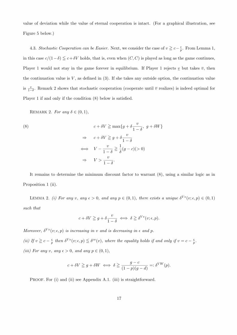
4.3. Stochastic Cooperation can be Easier. Next, we consider the case of v = c− εp . From Lemma 1,

in this case c/(1−δ) 5 c+δV holds, that is, even when (C,C) is played as long as the game continues,

Player 1 would not stay in the game forever in equilibrium. If Player 1 rejects v but takes v, then

the continuation value is V , as defined in (3). If she takes any outside option, the continuation value

is v1−δ . Remark 2 shows that stochastic cooperation (cooperate until v realizes) is indeed optimal for

Player 1 if and only if the condition (8) below is satisfied.

REMARK 2. For any δ ∈ (0, 1),

c + δV = max{g + δv

1 − δ, g + δW}(8)

⇒ c + δV = g + δv

1 − δ

⇐⇒ V − v

1 − δ= 1

δ(g − c)(> 0)

⇒ V >v

1 − δ.

It remains to determine the minimum discount factor to warrant (8), using a similar logic as in

Proposition 1 (ii).

LEMMA 2. (i) For any v, any ε > 0, and any p ∈ (0, 1), there exists a unique δV v(v; ε, p) ∈ (0, 1)

such that

c + δV = g + δv

1 − δ⇐⇒ δ = δV v(v; ε, p).

Moreover, δV v(v; ε, p) is increasing in v and is decreasing in ε and p.

(ii) If v = c − εp then δV v(v; ε, p) 5 δcv(v), where the equality holds if and only if v = c − ε

p .

(iii) For any v, any ε > 0, and any p ∈ (0, 1),

c + δV = g + δW ⇐⇒ δ = g − c

(1 − p)(g − d)=: δV W (p).

PROOF. For (i) and (ii) see Appendix A.1. (iii) is straightforward.

17

Note that δV W (p) does not depend on the mean v or the spread ε, since the exit behavior is the

same in both cooperation phase and punishment phase. We need to clarify when it is relevant, i.e.,

less than 1. By an easy computation, we have the following properties of δV W (p).

REMARK 3. (i) δV W (p) < 1 ⇐⇒ c > pg + (1 − p)d; and

(ii) δV W (p) 5 δcv(v) ⇐⇒ g−c(1−p)(g−d) 5 g−c

g−v ⇐⇒ v = pg + (1 − p)d.

Remark 3 (i) is important. This shows that (8) does not hold if c 5 pg+(1−p)d, since δV W (p) = 1

means that c + δV < g + δW for all δ ∈ (0, 1) and thus

c + δV < max{g + δv

1 − δ, g + δW}.

Therefore, although the increase of the mean v per se would not make cooperation impossible, increase

of the probability p of the good option makes stochastic cooperation impossible (by making c 5

pg + (1 − p)d). In this case, the minimum discount factor to sustain eternal cooperation δcW (v; ε, p)

reaches 1 at v = c − εp .

PROPOSITION 2. Take any v, any ε > 0, and any p ∈ (0, 1) such that v = c − εp .

Case 1: Take any p such that c > pg + (1 − p)d. Let v∗∗ := d + (g−d)εc−{pg+(1−p)d} .

(i) Stochastic cooperation is sustained if and only if{δ = δV W (p) if c − ε

p 5 v 5 v∗∗;δ = δV v(v; ε, p) if v∗∗ 5 v.

(ii) v∗∗ R pg + (1 − p)d ⇐⇒ pg + (1 − p)d R c − εp .

Case 2: If c 5 pg + (1 − p)d, then cooperation cannot be sustained for v = c − εp .

PROOF. For Case 1 (i), see Appendix A.1. (ii) is an easy computation. Case 2 is from Remark 3

(i) as derived in the text.

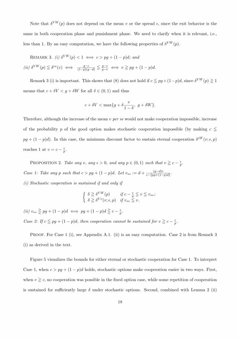
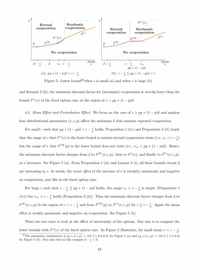
Figure 5 visualizes the bounds for either eternal or stochastic cooperation for Case 1. To interpret

Case 1, when c > pg + (1 − p)d holds, stochastic options make cooperation easier in two ways. First,

when v = c, no cooperation was possible in the fixed option case, while some repetition of cooperation

is sustained for sufficiently large δ under stochastic options. Second, combined with Lemma 2 (ii)

18

δ1

meanv

Eternalcooperation

Stochasticcooperation

No cooperation

δ

d − εp d c − ε

p

δcv(v)

v∗

δcW

δV v

(a): pg + (1 − p)d < c − εp

δ1

meanvd − ε

p c − εp

δ δcWδV W

δcv(v)

Eternalcooperation

Stochasticcooperation

No cooperation

pg + (1 − p)d

v∗∗

δV v

(b): c − εp 5 pg + (1 − p)d < c

Figure 5: Lower bound20when ε is small (a) and when ε is large (b).

and Remark 3 (ii), the minimum discount factor for (stochastic) cooperation is strictly lower than the

bound δcv(v) of the fixed option case, in the region of v > pg + (1 − p)d.

4.4. Mean Effect and Perturbation Effect. We focus on the case of c > pg + (1 − p)d and analyze

how distributional parameters (v, ε, p) affect the minimum δ that sustains repeated cooperation.

For small ε such that pg + (1 − p)d < c − εp holds, Proposition 1 (iv) and Proposition 2 (ii) imply

that the range of v that δcv(v) is the lower bound to sustain eternal cooperation exists (i.e., v∗ < c− εp)

but the range of v that δV W (p) is the lower bound does not exist (i.e., v∗∗ < pg + (1 − p)d). Hence,

the minimum discount factor changes from δ to δcW (v; ε, p), then to δcv(v), and finally to δV v(v; ε, p),

as v increases. See Figure 5 (a). From Proposition 1 (iii) and Lemma 2 (i), all these bounds except δ

are increasing in v. In words, the mean effect of the increase of v is (weakly) monotonic and negative

on cooperation, just like in the fixed option case.

For large ε such that c − εp 5 pg + (1 − p)d holds, the range v∗ < c − ε

p is empty (Proposition 1

(iv)) but v∗∗ > c− εp holds (Proposition 2 (ii)). Thus the minimum discount factor changes from δ to

δcW (v; ε, p) in the region of v < c − εp and from δV W (p) to δV v(v; ε, p) for v = c − ε

p . Again the mean

effect is weakly monotonic and negative on cooperation. See Figure 5 (b).

There are two ways to look at the effect of uncertainty of the options. One way is to compare the

lower bounds with δcv(v) of the fixed option case. As Figure 5 illustrates, for small mean v < c − εp ,

20The parameter combination is (g, c, d, ε, p) = (10, 7, 1, 0.8, 0.3) for Figure 5 (a) and (g, c, d, ε, p) = (10, 7, 1, 1.5, 0.3)for Figure 5 (b). Note also that in this example d − ε

p< 0.

19

δ1

ε=

0

?

ε up

pg + (1 − p)dv

δcW

δV v

6

¾EternalCooperation

No Cooperation

d c

Figure 6: Perturbation effect

the minimum discount factor for eternal cooperation is never below δcv(v) of the fixed option case.

However, for large v > c − εp or v > pg + (1 − p)d, Lemma 2 (ii) and Remark 3 (ii) imply that the

minimum discount factor that sustains stochastic cooperation is strictly below δcv(v), although the

repetition ends with probability p. Hence the uncertainty has a negative effect on cooperation when v

is low but a positive effect when v is high. This is because when v is small, the optimal exit strategy in

the cooperation phase is not to take any option, thus uncertainty only increases the value of deviation,

while when v is large, uncertainty increases the value of (stochastic) cooperation as well, and when

the mean v is very large, it only increases the cooperation value since Player 1 takes both options

after deviation.

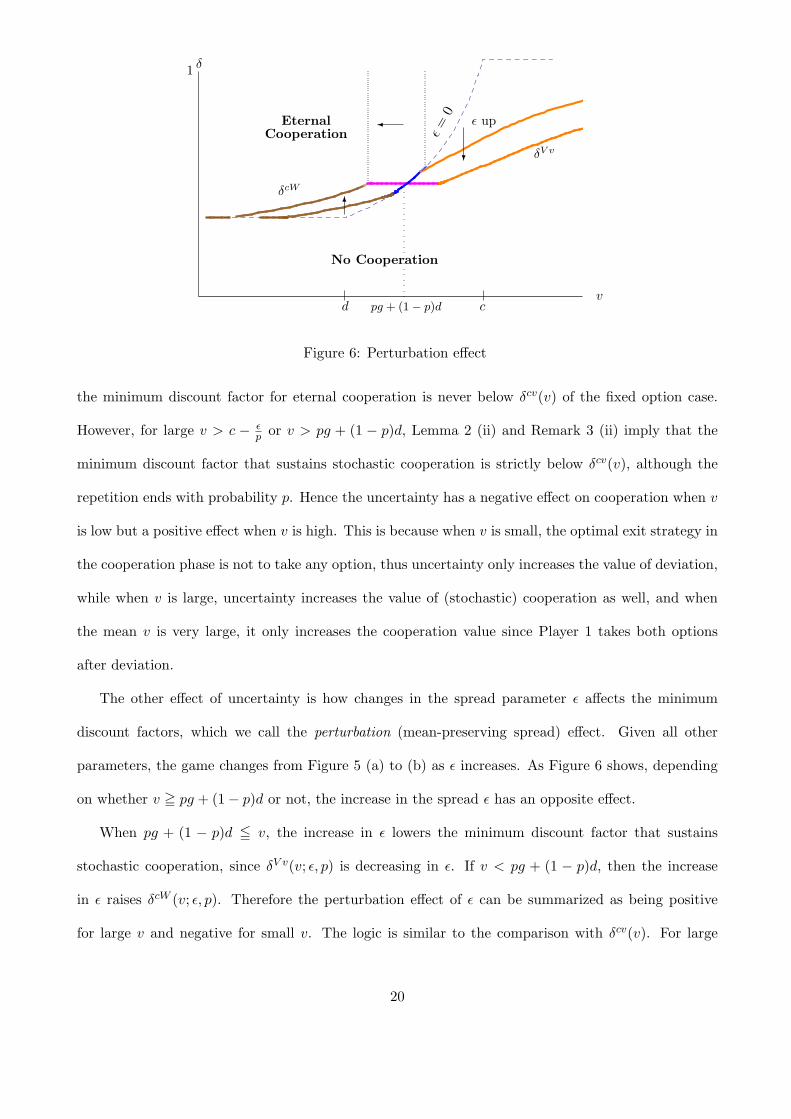
The other effect of uncertainty is how changes in the spread parameter ε affects the minimum

discount factors, which we call the perturbation (mean-preserving spread) effect. Given all other

parameters, the game changes from Figure 5 (a) to (b) as ε increases. As Figure 6 shows, depending

on whether v = pg + (1 − p)d or not, the increase in the spread ε has an opposite effect.

When pg + (1 − p)d 5 v, the increase in ε lowers the minimum discount factor that sustains

stochastic cooperation, since δV v(v; ε, p) is decreasing in ε. If v < pg + (1 − p)d, then the increase

in ε raises δcW (v; ε, p). Therefore the perturbation effect of ε can be summarized as being positive

for large v and negative for small v. The logic is similar to the comparison with δcv(v). For large

20

v’s, the increase in the spread raises either the value of stochastic cooperation only, or both the value

of stochastic cooperation and the value of deviation, while for low v’s, it only increases the value of

deviation. Therefore in the former case (where δV v(v; ε, p) is the relevant minimum discount factor),

the increase of the spread ε makes cooperation easier.

In addition, the range of v that admits eternal cooperation (v 5 c− εp) shrinks as ε increases. This

means also that eternal cooperation is more difficult to sustain as the spread ε increases.

The asymmetric effects of uncertainty at different levels of the mean lead to new economic im-

plications. Suppose that Player 1 is a worker and the volatility of the options comes from economic

conditions. Then workers who have a high-mean distribution of outside options become more coop-

erative as the economy becomes more volatile, in the sense that those with less patience can follow

stochastic cooperation. By contrast, workers with a low-mean distribution of outside options become

less cooperative. In addition, workers with intermediate-mean distributions, who could follow eternal

cooperation, may start stochastic cooperation as the spread of the outside options increases. Therefore,

even though the internal game parameter is stationary, the external perturbation of outside options

generates more shirking of “low-end” workers, more quits of “mid-level” workers, but more cooperation

from “high-end” workers (until they find next jobs). This is an interesting testable hypothesis.

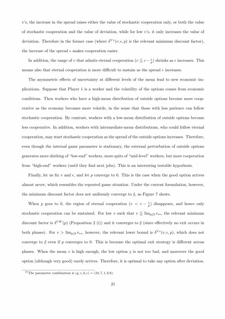
Finally, let us fix v and ε, and let p converge to 0. This is the case when the good option arrives

almost never, which resembles the repeated game situation. Under the current formulation, however,

the minimum discount factor does not uniformly converge to δ, as Figure 7 shows.

When p goes to 0, the region of eternal cooperation (v < c − εp) disappears, and hence only

stochastic cooperation can be sustained. For low v such that v 5 limp↓0 v∗∗, the relevant minimum

discount factor is δV W (p) (Proposition 2 (i)) and it converges to δ (since effectively no exit occurs in

both phases). For v > limp↓0 v∗∗, however, the relevant lower bound is δV v(v; ε, p), which does not

converge to δ even if p converges to 0. This is because the optimal exit strategy is different across

phases. When the mean v is high enough, the low option v is not too bad, and moreover the good

option (although very good) rarely arrives. Therefore, it is optimal to take any option after deviation.

21The parameter combination is (g, c, d, ε) = (10, 7, 1, 0.8).

21

δ1

p ↓ 0

v

δcW (p = 0.3)

δV W = δ

δV v

limp↓0 v∗∗

Stochastic cooperation≈ Eternal cooperation

d c

Figure 7: Convergence21of p to 0

Thus the existence of the low option (which does not converge to −∞) makes the dynamic game

different from a repeated game.

In general, there are two other possibilities when p goes to 0 (given that the mean is fixed). One is

that both v and v diverge to +∞ and −∞, and the other is that v and v converge to finite values. In

the former case, the game reduces to ordinary repeated game, since exit never occurs in both phases.

In the latter case, both options must converge to the mean, so that the game becomes a deterministic

option game. Therefore the current formulation takes an interesting middle ground.22

Note also that, even though the current formulation does not give δ for every v as p ↓ 0, the

minimum discount factor to sustain almost eternal cooperation is uniformly lower than δcv(v), since

limp↓0 v∗∗ = d + (g−d)εc−d > d. In this sense very small p makes cooperation easier.

4.5. General Distributions. Although of some theoretical interest, considering more than two (or a

continuum of) outside options as in job search theory would make the analysis more complex, without

giving us more insights than the binary option model. In this subsection we clarify that the main

results in the binary stochastic options are robust when we add more options.23

The essence of the analyses in the previous sections can be summarized as follows. In each phase

22It can be shown that changing p while keeping the variance of option values constant would result in the sameconvergence pattern as ours.

23An explicit analysis of finitely-many options and continuum of options are given in the working paper version of thispaper, Fujiwara-Greve and Yasuda (2011).

22

v 5 d − εp d − ε

p < v < v∗ v∗ 5 v < c − εp c − ε

p 5 v

Cooperation phase ∞ ∞ ∞ vreservation level

Punishment phase ∞ v v vreservation levelLower bound δ δcW (> δcv(v)) δcv(v) δV v(< δcv(v))

to sustain cooperation

Table 3: Optimal reservation levels under binary stochastic options when pg + (1 − p)d 5 c − εp

(cooperation phase or punishment phase), the optimal exit rule of Player 1 is a reservation strategy

such that she takes any option not less than a reservation level. This is because each option is a total

expected payoff after exit and thus can be compared in one dimension. Hence even with more options,

the optimal exit decision is a reservation strategy. Under the fixed option, there are only two possible

reservation levels, ∞ (not to take any option) and v (to take the option v), while under the binary

options, there are three. (See Tables 3 and 4.) Thus Player 1 can adjust the optimal reservation

levels in finer steps when there are more option values available. As the mean v of the outside options

increases, it becomes better to take some outside options, but the optimal reservation level in the

cooperation phase is never lower than that of the punishment phase, because the expected payoff in

the repeated Prisoner’s Dilemma is higher in the cooperation phase. These two properties are shown

in Tables 3 and 4 for the binary option case, and they hold for more than two options as well.

The above structure of the optimal exit decision rule is the key to the main results of the previous

analyses: difficulty of eternal cooperation and ease of stochastic cooperation under binary options as

compared to the case when the mean value is the fixed option.

When the mean is not so high, it is optimal to stay forever in the cooperation phase under both

fixed and binary options. After deviation, Player 1 can guarantee herself v1−δ in any case and may

increase the value of deviation when the optimal reservation level is above v, under binary distributions.

Therefore eternal cooperation becomes more difficult with stochastic options. See the second columns

of Tables 3 and 4. This logic holds for general distributions.

When the mean is high, it becomes better to take some options in the cooperation phase, which

means that the value of stochastic cooperation becomes greater than that of eternal cooperation.

23

v 5 d − εp d − ε

p < v < c − εp c − ε

p 5 v 5 v∗∗ v∗∗ < v

Coop. phase ∞ ∞ v v

Punish. phase ∞ v v v

Lower bound δ δcW (> δcv(v)) δV W δV v(< δcv(v))

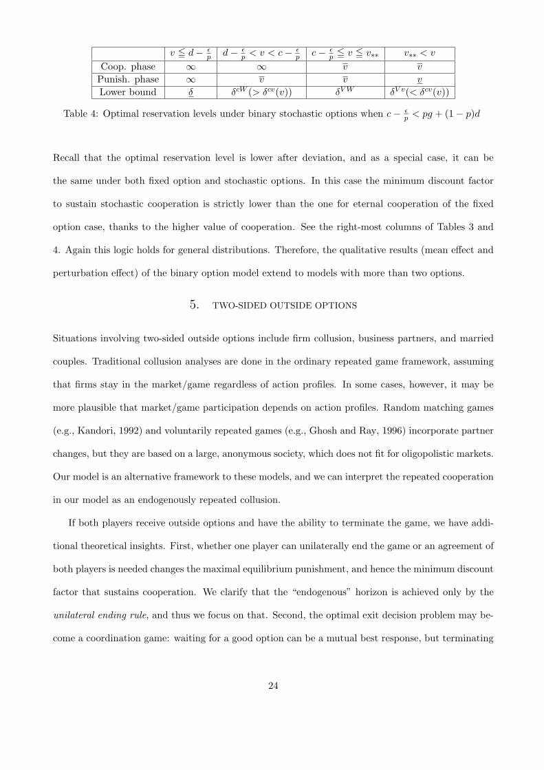
Table 4: Optimal reservation levels under binary stochastic options when c − εp < pg + (1 − p)d

Recall that the optimal reservation level is lower after deviation, and as a special case, it can be

the same under both fixed option and stochastic options. In this case the minimum discount factor

to sustain stochastic cooperation is strictly lower than the one for eternal cooperation of the fixed

option case, thanks to the higher value of cooperation. See the right-most columns of Tables 3 and

4. Again this logic holds for general distributions. Therefore, the qualitative results (mean effect and

perturbation effect) of the binary option model extend to models with more than two options.

5. TWO-SIDED OUTSIDE OPTIONS

Situations involving two-sided outside options include firm collusion, business partners, and married

couples. Traditional collusion analyses are done in the ordinary repeated game framework, assuming

that firms stay in the market/game regardless of action profiles. In some cases, however, it may be

more plausible that market/game participation depends on action profiles. Random matching games

(e.g., Kandori, 1992) and voluntarily repeated games (e.g., Ghosh and Ray, 1996) incorporate partner

changes, but they are based on a large, anonymous society, which does not fit for oligopolistic markets.

Our model is an alternative framework to these models, and we can interpret the repeated cooperation

in our model as an endogenously repeated collusion.

If both players receive outside options and have the ability to terminate the game, we have addi-

tional theoretical insights. First, whether one player can unilaterally end the game or an agreement of

both players is needed changes the maximal equilibrium punishment, and hence the minimum discount

factor that sustains cooperation. We clarify that the “endogenous” horizon is achieved only by the

unilateral ending rule, and thus we focus on that. Second, the optimal exit decision problem may be-

come a coordination game: waiting for a good option can be a mutual best response, but terminating

24

the game immediately by taking any option is also a mutual best response. Third, mutual immediate

exit constitutes the maximal equilibrium punishment, and hence, when the outside option value is

smaller than d, cooperation is easier than under the repeated game. Fourth, the payoff of stochastic

cooperation is lower than the one under the one-sided option model, because a player may be forced

to take a low option when the partner terminates the game. Therefore, the positive effect of stochastic

options on cooperation, due to the increase in the option value, is reduced under two-sided options.

5.1. Model. The model is essentially the same as the one in Sections 3-4, except that at the end of

each period, each player faces an outside option and decides whether to take it or not simultaneously.

We do not assume that the outside option values are necessarily the same across the players. There

are two possible ending rules for this model; the unilateral ending rule and the mutual agreement rule.

Under the unilateral ending rule, the repeated game ends if and only if at least one player chooses to

take an outside option. This is the common assumption in the voluntarily repeated game literature

as well (e.g., Ghosh and Ray, 1996). By contrast, the mutual agreement rule requires both players to

agree (i.e., to take own outside option simultaneously) to end the game. This is the case, for instance,

for marriage dissolutions in some countries. We assume that when the game ends, both players must

take the currently realized option.24 Therefore the point of the mutual agreement rule is that a single

player can refuse to end the game (and reject the current option for sure). The unilateral rule, by

contrast, allows a single player to force the partner to take his option.

The mutual agreement rule makes the game essentially the same as the ordinary repeated game,

since a player can refuse to terminate the game after any history, and can guarantee herself at least the

in-game punishment payoff. Therefore, we focus on the unilateral ending rule. Under the unilateral

ending rule, a player can strategically terminate the game but also may involuntarily be stuck with an

unwanted option as well. Hence we have different implications in this model, from both the one-sided

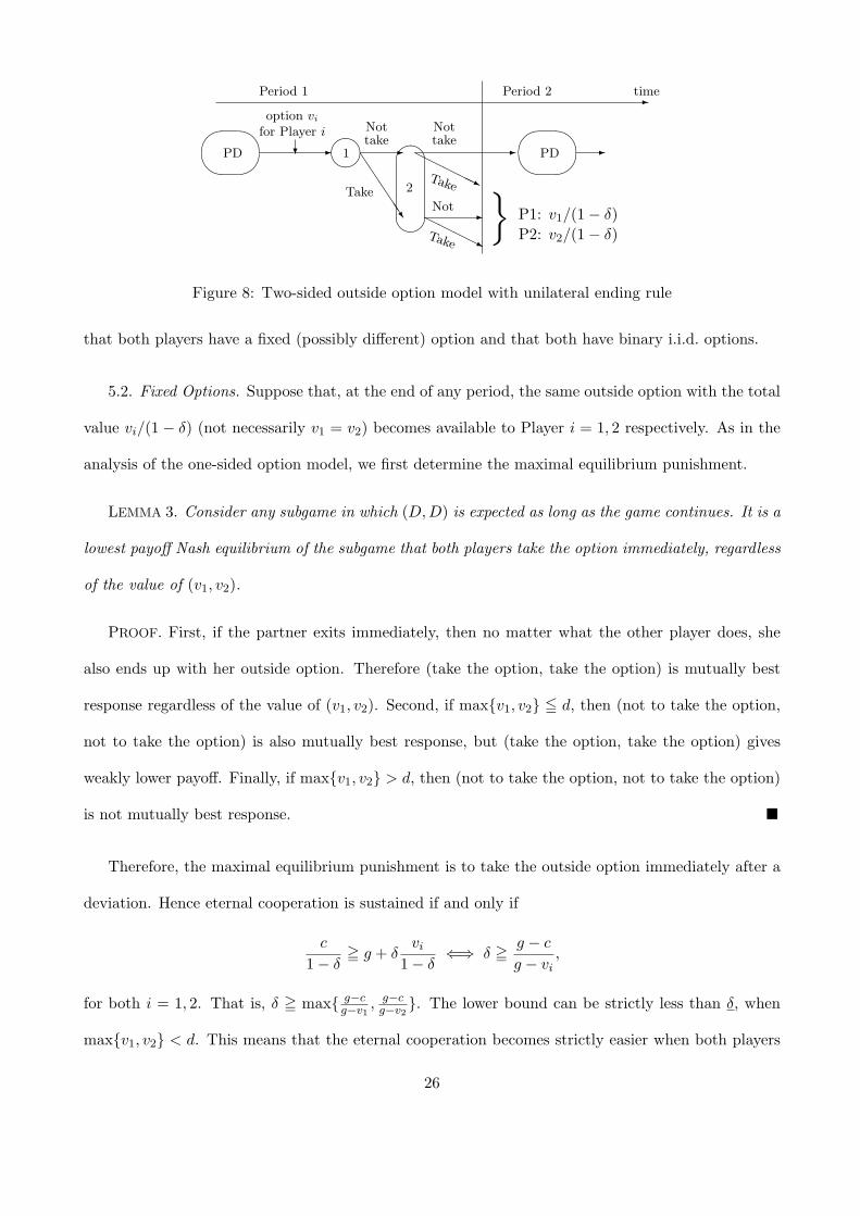
option model and the ordinary repeated game. The outline of the two-sided outside option model

with the unilateral ending rule is depicted in Figure 8.

To compare with the one-sided outside option models, we consider the same option structures:24An interpretation is that an option is a continuation value of one’s life and thus cannot avoid it.

25

-Period 1 Period 2 time

¾½

»¼PD -

option vi

for Player i

? µ´¶³1 -

JJ

JJJ

Nottake

Take

¶

µ

³

´2

-

Nottake

HHHHHjTake

-HHHHj

Not

Take

P1: v1/(1 − δ)P2: v2/(1 − δ)

}¾½

»¼PD -

Figure 8: Two-sided outside option model with unilateral ending rule

that both players have a fixed (possibly different) option and that both have binary i.i.d. options.

5.2. Fixed Options. Suppose that, at the end of any period, the same outside option with the total

value vi/(1 − δ) (not necessarily v1 = v2) becomes available to Player i = 1, 2 respectively. As in the

analysis of the one-sided option model, we first determine the maximal equilibrium punishment.

LEMMA 3. Consider any subgame in which (D,D) is expected as long as the game continues. It is a

lowest payoff Nash equilibrium of the subgame that both players take the option immediately, regardless

of the value of (v1, v2).

PROOF. First, if the partner exits immediately, then no matter what the other player does, she

also ends up with her outside option. Therefore (take the option, take the option) is mutually best

response regardless of the value of (v1, v2). Second, if max{v1, v2} 5 d, then (not to take the option,

not to take the option) is also mutually best response, but (take the option, take the option) gives

weakly lower payoff. Finally, if max{v1, v2} > d, then (not to take the option, not to take the option)

is not mutually best response. ¥

Therefore, the maximal equilibrium punishment is to take the outside option immediately after a

deviation. Hence eternal cooperation is sustained if and only if

c

1 − δ= g + δ

vi

1 − δ⇐⇒ δ = g − c

g − vi,

for both i = 1, 2. That is, δ = max{ g−cg−v1

, g−cg−v2

}. The lower bound can be strictly less than δ, when

max{v1, v2} < d. This means that the eternal cooperation becomes strictly easier when both players

26

1 \ 2 v + εp v − ε

1−p

v + εp pρ p(1 − ρ)

v − ε1−p p(1 − ρ) 1 − 2p + pρ

Table 5: Two-sided (correlated) outside option distribution (p 5 1/2, ρ ∈ (0, 1])

have fixed outside options, than when only one or no player has a (fixed) outside option.

The point is that, when only Player 1 has an outside option, subgame perfection requires that

Player 1 optimizes in the punishment phase, and thus the punishment cannot be stricter than that

of the repeated game. By contrast, when both players have an outside option, Lemma 3 shows that

immediate exit is the maximal equilibrium punishment, regardless of the value of the options, and this

punishment can be stricter than mutual defection. Note that this property continues to hold when

the outside options are stochastic.

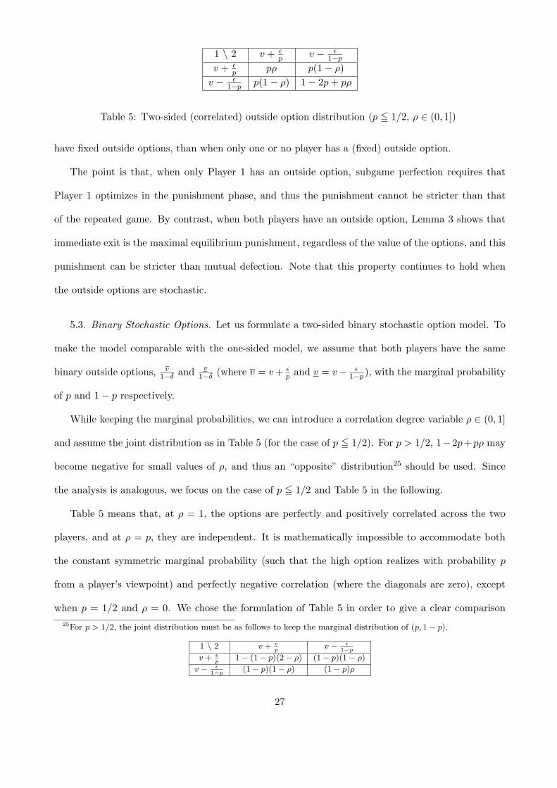
5.3. Binary Stochastic Options. Let us formulate a two-sided binary stochastic option model. To

make the model comparable with the one-sided model, we assume that both players have the same

binary outside options, v1−δ and v

1−δ (where v = v + εp and v = v− ε

1−p), with the marginal probability

of p and 1 − p respectively.

While keeping the marginal probabilities, we can introduce a correlation degree variable ρ ∈ (0, 1]

and assume the joint distribution as in Table 5 (for the case of p 5 1/2). For p > 1/2, 1−2p+pρ may

become negative for small values of ρ, and thus an “opposite” distribution25 should be used. Since

the analysis is analogous, we focus on the case of p 5 1/2 and Table 5 in the following.

Table 5 means that, at ρ = 1, the options are perfectly and positively correlated across the two

players, and at ρ = p, they are independent. It is mathematically impossible to accommodate both

the constant symmetric marginal probability (such that the high option realizes with probability p

from a player’s viewpoint) and perfectly negative correlation (where the diagonals are zero), except

when p = 1/2 and ρ = 0. We chose the formulation of Table 5 in order to give a clear comparison25For p > 1/2, the joint distribution must be as follows to keep the marginal distribution of (p, 1 − p).

1 \ 2 v + εp

v − ε1−p

v + εp

1 − (1 − p)(2 − ρ) (1 − p)(1 − ρ)

v − ε1−p

(1 − p)(1 − ρ) (1 − p)ρ

27

with the one-sided outside option model.

With uncertainty, the important difference from the one-sided option model is that a player may

end up taking the low option because the partner received the high option and took it to terminate

the game, when the realizations are not perfectly correlated. This reduces the expected payoff as

compared to the one-sided stochastic outside option case.

Suppose that (C,C) is expected as long as the game continues. We first show that the players’

optimal exit decision problem may become a coordination game, and then focus on the payoff-dominant

stationary action profile to be sustained, to derive the lowest δ.

If the partner does not take any option, then the ex ante expected payoff is the same as the one-

sided option case. Thus, consider the case that the partner has the reservation level v. Then using

the same reservation level v gives the following ex ante total expected payoff.

(9) Vv(ρ) = pv

1 − δ+ p(1 − ρ)

v

1 − δ+ {1 − p − p(1 − ρ)}{c + δVv(ρ)}.

To explain, the first term is the continuation value when the high option realizes (with probability p)

for this player, the second term is the continuation value when the low option realizes but the partner

received the high option and terminated the game (with probability p(1−ρ)), and the last term is the

continuation value when both players received the low option so that the game continues. Note also

that when the options are perfectly positively correlated (ρ = 1), we have that Vv(1) = V .

Similarly, when the partner has the reservation level v, not taking any option (having reservation

level ∞) gives

(10) V∞(ρ) = p{

ρv

1 − δ+ (1 − ρ)

v

1 − δ

}+ (1 − p){c + δV∞(ρ)}.

To explain, when the partner terminates the game (with probability p), the continuation value is v

with probability ρ and v with probability 1 − ρ. With probability 1 − p the partner does not receive

the high outside option and the game continues.

The total expected payoffs of the two players, of various combinations of exit strategies in the

cooperation phase, are summarized in Table 6. (Later we show that exiting immediately in the

cooperation phase is never optimal under two-sided outside options.)

28

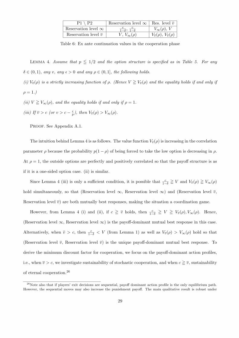
P1 \ P2 Reservation level ∞ Res. level v

Reservation level ∞ c1−δ , c

1−δ V∞(ρ), V

Reservation level v V , V∞(ρ) Vv(ρ), Vv(ρ)

Table 6: Ex ante continuation values in the cooperation phase

LEMMA 4. Assume that p 5 1/2 and the option structure is specified as in Table 5. For any

δ ∈ (0, 1), any v, any ε > 0 and any ρ ∈ (0, 1], the following holds.

(i) Vv(ρ) is a strictly increasing function of ρ. (Hence V = Vv(ρ) and the equality holds if and only if

ρ = 1.)

(ii) V = V∞(ρ), and the equality holds if and only if ρ = 1.

(iii) If v > c (or v > c − εp), then Vv(ρ) > V∞(ρ).

PROOF. See Appendix A.1.

The intuition behind Lemma 4 is as follows. The value function Vv(ρ) is increasing in the correlation

parameter ρ because the probability p(1− ρ) of being forced to take the low option is decreasing in ρ.

At ρ = 1, the outside options are perfectly and positively correlated so that the payoff structure is as

if it is a one-sided option case. (ii) is similar.

Since Lemma 4 (iii) is only a sufficient condition, it is possible that c1−δ = V and Vv(ρ) = V∞(ρ)

hold simultaneously, so that (Reservation level ∞, Reservation level ∞) and (Reservation level v,

Reservation level v) are both mutually best responses, making the situation a coordination game.

However, from Lemma 4 (i) and (ii), if c = v holds, then c1−δ = V = Vv(ρ), V∞(ρ). Hence,

(Reservation level ∞, Reservation level ∞) is the payoff-dominant mutual best response in this case.

Alternatively, when v > c, then c1−δ < V (from Lemma 1) as well as Vv(ρ) > V∞(ρ) hold so that

(Reservation level v, Reservation level v) is the unique payoff-dominant mutual best response. To

derive the minimum discount factor for cooperation, we focus on the payoff-dominant action profiles,

i.e., when v > c, we investigate sustainability of stochastic cooperation, and when c = v, sustainability

of eternal cooperation.26

26Note also that if players’ exit decisions are sequential, payoff dominant action profile is the only equilibrium path.However, the sequential moves may also increase the punishment payoff. The main qualitative result is robust under

29

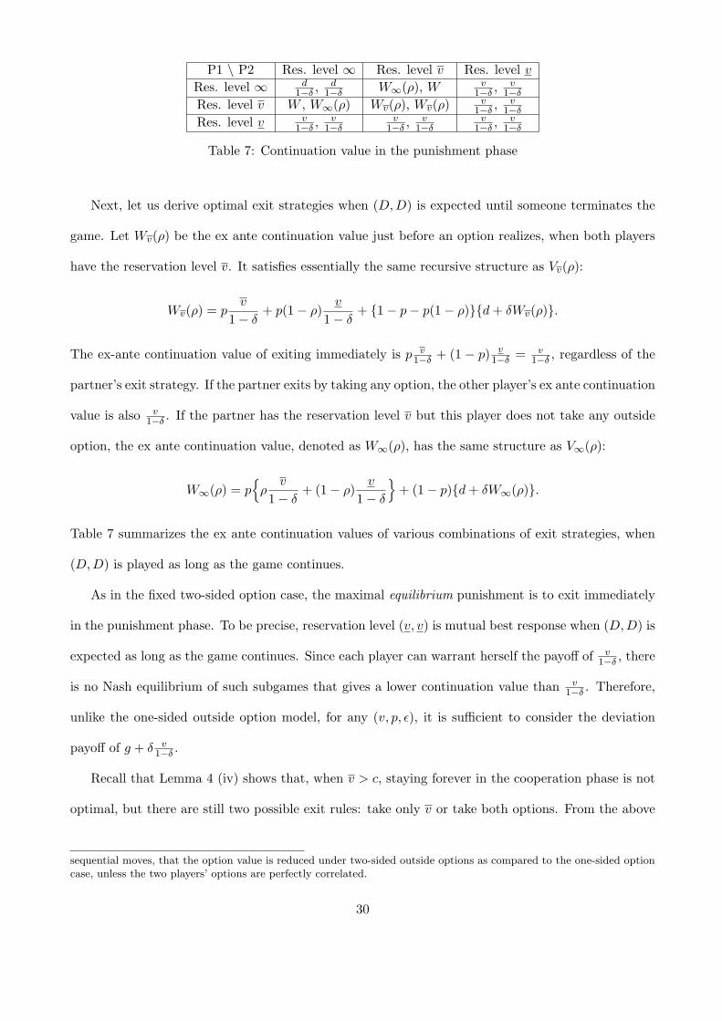
P1 \ P2 Res. level ∞ Res. level v Res. level v

Res. level ∞ d1−δ , d

1−δ W∞(ρ), W v1−δ , v

1−δ

Res. level v W , W∞(ρ) Wv(ρ), Wv(ρ) v1−δ , v

1−δ

Res. level v v1−δ , v

1−δv

1−δ , v1−δ

v1−δ , v

1−δ

Table 7: Continuation value in the punishment phase

Next, let us derive optimal exit strategies when (D,D) is expected until someone terminates the

game. Let Wv(ρ) be the ex ante continuation value just before an option realizes, when both players

have the reservation level v. It satisfies essentially the same recursive structure as Vv(ρ):

Wv(ρ) = pv

1 − δ+ p(1 − ρ)

v

1 − δ+ {1 − p − p(1 − ρ)}{d + δWv(ρ)}.

The ex-ante continuation value of exiting immediately is p v1−δ + (1 − p) v

1−δ = v1−δ , regardless of the

partner’s exit strategy. If the partner exits by taking any option, the other player’s ex ante continuation

value is also v1−δ . If the partner has the reservation level v but this player does not take any outside

option, the ex ante continuation value, denoted as W∞(ρ), has the same structure as V∞(ρ):

W∞(ρ) = p{

ρv

1 − δ+ (1 − ρ)

v

1 − δ

}+ (1 − p){d + δW∞(ρ)}.

Table 7 summarizes the ex ante continuation values of various combinations of exit strategies, when

(D,D) is played as long as the game continues.

As in the fixed two-sided option case, the maximal equilibrium punishment is to exit immediately

in the punishment phase. To be precise, reservation level (v, v) is mutual best response when (D,D) is

expected as long as the game continues. Since each player can warrant herself the payoff of v1−δ , there

is no Nash equilibrium of such subgames that gives a lower continuation value than v1−δ . Therefore,

unlike the one-sided outside option model, for any (v, p, ε), it is sufficient to consider the deviation

payoff of g + δ v1−δ .

Recall that Lemma 4 (iv) shows that, when v > c, staying forever in the cooperation phase is not

optimal, but there are still two possible exit rules: take only v or take both options. From the above

sequential moves, that the option value is reduced under two-sided outside options as compared to the one-sided optioncase, unless the two players’ options are perfectly correlated.

30

argument, stochastic cooperation is sustained if and only if

(11) c + δVv(ρ) = g + δv

1 − δ.

Moreover, by the same logic as Remark 2, (11) implies that Vv(ρ) > v1−δ . That is, exiting immediately

in the cooperation phase is not optimal so that indeed stochastic cooperation is optimal.

We are ready to determine the minimum discount factor. When c = v, eternal cooperation is

sustained as an outcome of a SPE in the two-sided stochastic option model if and only if

c

1 − δ= g + δ

v

1 − δ⇐⇒ δ = δcv(v),

while when v > c, stochastic cooperation is sustained as an outcome of a SPE if and only if (11) holds.

From Lemma 4 (i), c + δV = c + δVv(ρ). Hence the lower bound of δ that warrants (11) is never

smaller than δV v(v; ε, p) which satisfies c + δV = g + δ v1−δ . Since the case of p > 1/2 is analogous, we

have the following result.

PROPOSITION 3. For any v, any ε > 0, any p ∈ (0, 1), and any ρ ∈ (0, 1], the two-sided stochastic

outside options specified as in Table 5 (when p 5 1/2) or the table in the footnote 25 (when p > 1/2)

make eternal cooperation easier but stochastic cooperation more difficult than the case of the binary

one-sided options. Specifically,

(i) if c = v, then eternal cooperation is sustained if and only if δ = δcv(v);

(ii) if v > c, then there exists δV v2(v; ε, p, ρ) ∈ [δV v(v; ε, p), 1) such that stochastic cooperation is

sustained if and only if δ = δV v2(v; ε, p, ρ); and

(iii) the lower bound δV v2(v; ε, p, ρ) is decreasing in the spread ε and in the degree ρ of (positive)

correlation across players.

PROOF. (i) is shown in the text. (ii) is analogous to the existence of δV v(v; ε, p) in the proof of

Lemma 2 (i). (iii) is implied by the fact that Vv(ρ) is increasing in ε and ρ. ¥

Proposition 3 (iii) implies that the perturbation effect of ε is robust under two-sided outside

options. An additional effect of ρ means that more positive correlation across the partners enhances

31

δ1

v

δ

d

Two-sided δcv (v)

δcW

c − εp

Eternal cooperation Stochastic cooperation

δcv(v)

Two-sided δ

V v2

One-sided δ

V v

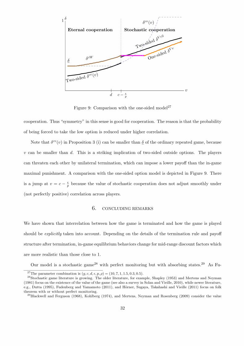
Figure 9: Comparison with the one-sided model27

cooperation. Thus “symmetry” in this sense is good for cooperation. The reason is that the probability

of being forced to take the low option is reduced under higher correlation.

Note that δcv(v) in Proposition 3 (i) can be smaller than δ of the ordinary repeated game, because

v can be smaller than d. This is a striking implication of two-sided outside options. The players

can threaten each other by unilateral termination, which can impose a lower payoff than the in-game

maximal punishment. A comparison with the one-sided option model is depicted in Figure 9. There

is a jump at v = c − εp because the value of stochastic cooperation does not adjust smoothly under

(not perfectly positive) correlation across players.

6. CONCLUDING REMARKS

We have shown that interrelation between how the game is terminated and how the game is played

should be explicitly taken into account. Depending on the details of the termination rule and payoff

structure after termination, in-game equilibrium behaviors change for mid-range discount factors which

are more realistic than those close to 1.

Our model is a stochastic game28 with perfect monitoring but with absorbing states.29 As Fu-

27The parameter combination is (g, c, d, ε, p, ρ) = (10, 7, 1, 1.5, 0.3, 0.5).28Stochastic game literature is growing. The older literature, for example, Shapley (1953) and Mertens and Neyman

(1981) focus on the existence of the value of the game (see also a survey in Solan and Vieille, 2010), while newer literature,e.g., Dutta (1995), Fudenberg and Yamamoto (2011), and Horner, Sugaya, Takahashi and Vieille (2011) focus on folktheorem with or without perfect monitoring.

29Blackwell and Ferguson (1968), Kohlberg (1974), and Mertens, Neyman and Rosenberg (2009) consider the value

32

denberg and Yamamoto (2011) point out, absorbing states can make the structure of equilibria very

different from that of repeated games, and the existing folk theorems (e.g., Dutta, 1995) of stochastic

games do not apply. Specifically, our model violates both Assumptions A1 and A2 in Dutta (1995).

Nevertheless, we have constructed SPEs with non-myopic action profiles for sufficiently large δ.

Our equilibrium analysis involves an optimal stopping problem with controls. Quah and Strulovici

(2011) give a general analysis of such problems with the focus on the effect of discount factor, while

we focus on the effect of outside options. Their monotonicity result holds in our context, in the sense

that both the on-path value function and the punishment value function, with endogenous optimal

reservation levels, are increasing in δ. See, for example, Figure 4.30 In addition, we analyze how the

on-path value function and the deviation value function change, as the structure of outside options

changes, to derive the effect on the minimum discount factor that sustains cooperation.

Our logic of finitely repeated cooperation is different from that of Neyman (1999), which is based on

incomplete information of the horizon. Our game is of complete information and the stochastic outside

options make the horizon uncertain endogenously. Furusawa and Kawakami (2008) also establish

cooperation until an uncertain period, but that is due to stochastic arrival of the ending option of the

game, not the stochastic value of the options.

There are many economic implications from our game-theoretic analysis. First, having outside

options per se does not mean collapse of long-term cooperative relationships. We observe such phe-

nomena often. Even though junior workers may leave first jobs eventually, they may still make effort

at the current firms. Doctors and researchers have also outside options, but as long as they choose to

stay at the current institution, they work hard. Second, work incentives under economic fluctuations

depend on the distribution of outside options (potential wage offers). For example, in good times when

workers have high-mean distributions of possible wage offers, fluctuation of potential offers enhances

cooperation/effort in the current relationship, to wait for attractive offers. Thus firm performance can

be improved in a more volatile labor market (although workers do not stay forever). By contrast, when

of zero-sum stochastic games with absorbing states. Rosenthal and Rubinstein (1984) analyze the “ruin game” withabsorbing states, where the game ends if a player fails to accumulate a certain level of payoffs.

30A general proof is found in Fujiwara-Greve and Yasuda (2011).

33

the economy is bad and workers have low-mean distributions of potential wage offers, the volatility

effect is opposite and may amplify the economic downturn.

In this paper we only considered outside options which are independent from the action profile or

the payoff within the repeated game, to address the effect of the existence of options and the ability

to terminate a repeated interaction. The independence assumption is plausible for example when the

actions or payoffs in a relationship are not observable to outsiders. Since positively correlated outside

options to in-game performance would enhance cooperation obviously, our contribution is that we

showed that even under independent outside options, fluctuation or two-sidedness of outside options

enhances cooperation. An interesting extension is a negative correlation between one’s payoff within

the current interaction and outside options. For example, investing in firm-specific human capital may

increase a worker’s payoff in the current firm but may decrease her payoff when she moves to another

firm. Then the cooperation incentive is not obvious.

Extensions of outside option structure in the direction of serial correlations may not give us new

insights. Consider, for example, a Markov binary distribution such that the previous period realization

influences this period probabilities of outside options. On one hand, if the high option is not worth

taking, the game is effectively an ordinary repeated game. On the other hand, if the high option is

worth taking, it must be taken at the first opportunity, which implies that the next period option

distribution is the one after a realization of the low option. This makes the option distribution the

same after the first period, as long as the game continues.31 Therefore, in either case, the analysis is

essentially the same as our i.i.d. model.

Lastly, let us mention an interesting extension to address a political economy problem, or a principal

vs. two agents problem, which endogenizes the outside option. Consider a two-party system, where

the constituency is the principal, an agent is the currently governing party, and the opposition party

is the unique outside option for the principal. The threat to switch to the opposition may affect how

the incumbent party makes effort for the constituency. At the same time, if the cooperation from the

incumbent is too good, the threat to change to the opposition may become non-credible, backfiring31If we can interpret the first period of the game also the one following the low option, since otherwise the game is not

started, then the probability structure is completely i.i.d.

34

vc − ε

p

d + ε1−p

0

d − εp

δ

d + ε(1−δ)(1−p)

v1−δ

> W

v1−δ

< W

Figure 10: Comparison between v1−δ and W

the incentive. A promise from the opposition party (the value of outside option) can also matter, but,

if the change of power occurs, the same incentive problem arises. In this way, the existence and the

structure of outside options are important in many contexts.

APPENDIX

A.1. Proofs. THE PROOF OF PROPOSITION 1: (ii) By the definition, we can solve W explicitly as

(12) W =pv + ε + (1 − p)(1 − δ)d{1 − δ(1 − p)}(1 − δ)

.

Hence, for any ε > 0 and any p ∈ (0, 1), a straightforward computation yields

(13)v

1 − δ= W ⇐⇒ v = d +

ε

(1 − δ)(1 − p).

The bound to v in (13) is increasing in δ and takes the minimum value d + ε1−p at δ = 0. Hence, if

d − εp < v 5 d + ε

1−p , then v1−δ < W holds for any δ ∈ (0, 1). Thus, in this case, the optimal exit

decision after deviation is to wait for v. See Figure 10.

Looking at the threshold as a function of v (which defines δP (v) := 1− ε(1−p)(v−d)), it is increasing

in v, meaning that the optimal deviation value max{g + δ v1−δ , g + δW} becomes g + δ v

1−δ for a

wider range of δ as v increases. As discussed in the text, at v∗ such that δP (v∗) = δcv(v∗), c1−δ ,

g + δ v1−δ , and g + δW all intersect, thus when v exceeds v∗, Player 1 cooperates if and only if

35

c1−δ = g + δ v

1−δ ⇐⇒ δ = δcv(v). (Recall Figure 4.) Note also that, since the on-path value c/(1 − δ)

is strictly less than max{g + δ v1−δ , g + δW} at δ = 0, v∗ must make δP (v) > 0, that is v∗ > d + ε

1−p .

For d+ ε1−p < v 5 c− ε

p (note that this interval might be empty), (13) implies that the relationship

between v1−δ and W changes as follows.{ v

1−δ = W if δ 5 δP (v);v

1−δ < W if δP (v) < δ < 1.

Consider the case of d − εp < v < v∗. From (12), c

1−δ = g + δW is equivalent to

0 5 −δ2(1 − p)(g − d) + δ{(1 − p)(g − d − c) + g − pv − ε} − (g − c) =: f(δ).

Hence f(0) = −(g − c) < 0. It is straightforward to show that f(1) = p{c − εp − v)} > 0.32 Since f

is a concave function of δ, f(1) > 0 implies that there exists a unique δcW (v; ε, p) ∈ (0, 1) such that

f(δ) = 0 (which is equivalent to c1−δ = g + δW ) if and only if δ = δcW (v; ε, p). δcW (v; ε, p) > δcv(v) is

straightforward from the fact that g + δW > g + δ v1−δ .

Moreover, f(δ) is decreasing in v and ε, for any δ > 0. Thus δcW (v; ε, p) is increasing in v and ε.

This proves (iii).

Finally, Player 2 follows eternal cooperation if and only if

c

1 − δ= g + δ(1 − p)d + δ2(1 − p)2d + · · · = g +

δ(1 − p)d1 − δ(1 − p)

,

since Player 1 terminates the game with probability p after deviation. The above condition is weaker

than Player 1’s condition, since

W − (1 − p)d1 − δ(1 − p)

=pv + ε

(1 − δ){1 − δ(1 − p)}> 0. ¥

THE PROOF OF LEMMA 2: (i) From the definition of V , we can solve V explicitly as

(14) V =pv + ε + (1 − p)(1 − δ)c{1 − δ(1 − p)}(1 − δ)

.

Therefore, c + δV = g + δ v1−δ is equivalent to

0 5 −δ2(1 − p)(g − v) + δ{g − c + ε + (1 − p)(g − v)} − (g − c) =: h(δ).32This also shows that when v = c− ε

p, f(1) = 0. If c 5 pg + (1− p)d also holds, then f ′(1) = −(1− p)(c− d) + p{g −

(v + εp)} = 0, so that no δ ∈ (0, 1) sustains eternal cooperation as soon as v reaches c − ε

p.

36

0.0 0.2 0.4 0.6 0.8

5

10

15

20

25

30

35

δ

g + δ v1−δ

c + δV c1−δ

¾

?

δV v

?

δcv

Figure 11: δV v(v; ε, p) 5 δcv(v) when v = c − εp33

Although the coefficient of δ2 can be of any sign, h is a quadratic function of δ, h(0) = −(g − c) < 0,

and h(1) = ε > 0. Therefore there exists a unique δV v(v; ε, p) ∈ (0, 1) above which h(δ) is positive.

Notice that h(δ) is a decreasing function of v and p and an increasing function of ε, given δ. Hence

δV v(v; ε, p) must increase in v and p, in order to keep h(δV v(v; ε, p)) = 0. Similarly, δV v(v; ε, p) is

decreasing in ε.

(ii) Recall that δcv(v) equates c1−δ = g + δ v

1−δ . If v = c − εp , then c + δV = c

1−δ = c + δ c1−δ by (4),

hence the value function of stochastic cooperation intersects with the function of g + δ v1−δ at a lower

δ than c1−δ does, i.e., δV v(v; ε, p) 5 δcv(v) holds. See Figure 11. ¥

THE PROOF OF PROPOSITION 2 (i): Since δV v(v; ε, p) is never greater than δcv(v) (Lemma 2 (ii)),

we should check when δV W (p) is less than δcv(v) and when δV v(v; ε, p) = max{δV v(v; ε, p), δV W (p)}.

The following Lemma is straightforward.

LEMMA 5. (a) δV W (p) R δcv(v) ⇐⇒ pg + (1 − p)d R v. (Easy computation.)

(b) δV W (p) R δP (v) ⇐⇒ δV W (p) R δV v(v; ε, p). (See Figure 12.) Hence,

δV W (p) 5 δP (v) ⇐⇒ max{δV v(v; ε, p), δV W (p)} = δV v(v; ε, p).

(c) δV W (p) R δP (v) ⇐⇒ v∗∗ = d + (g−d)εc−{pg+(1−p)d} R v. (Easy computation.)

From these, we can conclude that, if v 5 v∗∗, then δV W (p) = δP (v) which implies that max{δV v(v; ε, p),

δV W (p)} = δV W (p). If v > v∗∗, then δV W < δP (v) so that max{δV v(v; ε, p), δV W (p)} = δV v(v; ε, p).33The parameter combination is (g, c, d, v, ε, p) = (10, 7, 1, 5, 1, 0.3).34The parameter combination is (g, c, d, ε, p) = (10, 7, 1, 1, 0.2) and v = 3 (left) and v = 9 (right).

37

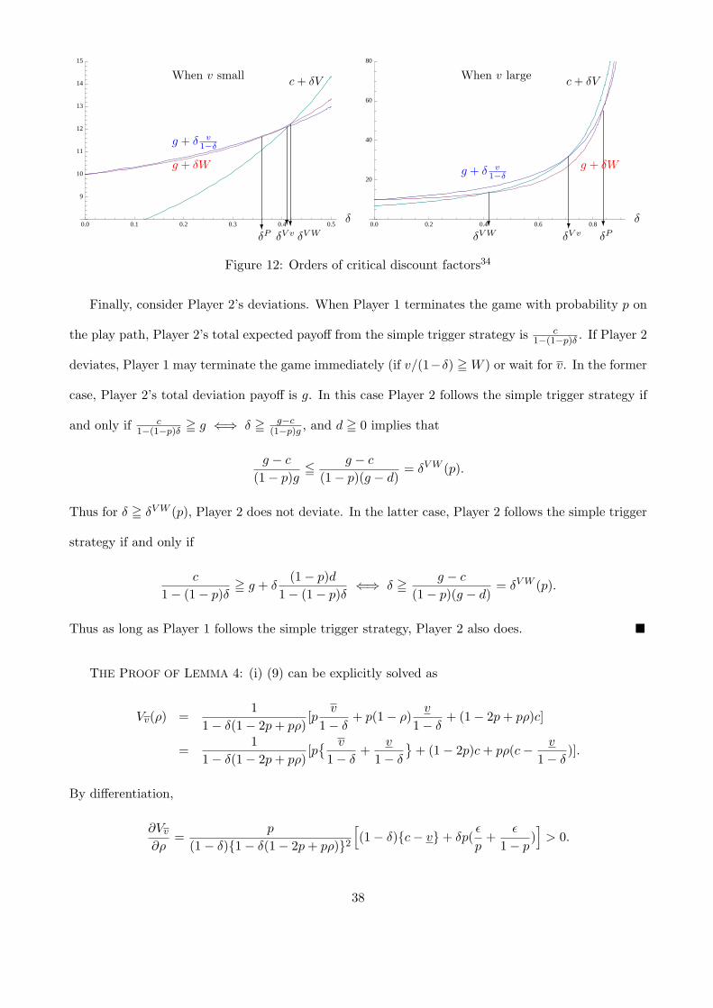
0.0 0.1 0.2 0.3 0.4 0.5

9

10

11

12

13

14

15

g + δ v1−δ

g + δW

c + δV

δ?δP

?δV v

?δV W

When v small

0.0 0.2 0.4 0.6 0.8

20

40

60

80

When v large

g + δ v1−δ

g + δW

c + δV

δ?δP

?δV v

?δV W

Figure 12: Orders of critical discount factors34

Finally, consider Player 2’s deviations. When Player 1 terminates the game with probability p on

the play path, Player 2’s total expected payoff from the simple trigger strategy is c1−(1−p)δ . If Player 2

deviates, Player 1 may terminate the game immediately (if v/(1−δ) = W ) or wait for v. In the former

case, Player 2’s total deviation payoff is g. In this case Player 2 follows the simple trigger strategy if

and only if c1−(1−p)δ = g ⇐⇒ δ = g−c

(1−p)g , and d = 0 implies that

g − c

(1 − p)g5 g − c

(1 − p)(g − d)= δV W (p).

Thus for δ = δV W (p), Player 2 does not deviate. In the latter case, Player 2 follows the simple trigger

strategy if and only if

c

1 − (1 − p)δ= g + δ

(1 − p)d1 − (1 − p)δ

⇐⇒ δ = g − c

(1 − p)(g − d)= δV W (p).

Thus as long as Player 1 follows the simple trigger strategy, Player 2 also does. ¥

THE PROOF OF LEMMA 4: (i) (9) can be explicitly solved as

Vv(ρ) =1

1 − δ(1 − 2p + pρ)[p

v

1 − δ+ p(1 − ρ)

v

1 − δ+ (1 − 2p + pρ)c]

=1

1 − δ(1 − 2p + pρ)[p

{ v

1 − δ+

v

1 − δ

}+ (1 − 2p)c + pρ(c − v

1 − δ)].

By differentiation,

∂Vv

∂ρ=

p

(1 − δ){1 − δ(1 − 2p + pρ)}2

[(1 − δ){c − v} + δp(

ε

p+

ε

1 − p)]

> 0.

38

(ii) From definitions,

V − V∞(ρ) = pv

1 − δ+ (1 − p)(c + δV )

−[pρv

1 − δ+ p(1 − ρ)

v

1 − δ+ (1 − p){c + δV∞(ρ)}]

= (1 − p)δ{V − V∞(ρ)} + p(1 − ρ){ v

1 − δ− v

1 − δ}

=p(1 − ρ)

1 − δ(1 − p)

{ v

1 − δ− v

1 − δ

}.

Therefore V = V∞(ρ) for any ρ ∈ (0, 1] and the equality holds if and only if ρ = 1.

(iii) From (9) and (10), we have

Vv(ρ) − V∞(ρ) = pv

1 − δ+ p(1 − ρ)

v

1 − δ+ {1 − p − p(1 − ρ)}{c + δVv(ρ)}

−[pρ

v

1 − δ+ p(1 − ρ)

v

1 − δ+ (1 − p){c + δV∞(ρ)}

]{1 − δ(1 − p)}{Vv(ρ) − V∞(ρ)} = p(1 − ρ)

[ v

1 − δ− {c + δVv(ρ)}

].

Therefore Vv(ρ) > V∞(ρ) if and only if v1−δ > c + δVv(ρ) holds. From (9),

c + δVv(ρ) = c + δ[p

v

1 − δ+ p(1 − ρ)

v

1 − δ+ {1 − p − p(1 − ρ)}{c + δVv(ρ)}

]⇐⇒ [1 − δ{1 − p − p(1 − ρ)}]{c + δVv(ρ)} = c + δ

[p

v

1 − δ+ p(1 − ρ)

v

1 − δ

]⇐⇒ c + δVv(ρ) =

c + δ[p v

1−δ + p(1 − ρ) v1−δ

]1 − δ + δp + δp(1 − ρ)

.(15)

Note that c < v implies that

c + δ[p

v

1 − δ+ p(1 − ρ)

v

1 − δ

]< (1 − δ)

v

1 − δ+ δp

v

1 − δ+ δp(1 − ρ)

v

1 − δ

Hence the RHS of (15) is less than v1−δ . ¥

A.2. Ex Post Optimal Exit Decisions. We show that the optimization problem after a realization of

an option gives exactly the same condition as Lemma 1. Suppose that Player 1 is at the decision node

where v is realized and there has been no Defection in the past. If she does not take this option, her

continuation payoff is max{ c1−δ , c + δV }, since she can optimize from the next period on. If v 5 c,

then v1−δ 5 c

1−δ = max{ c1−δ , c + δV } by (4). Thus she would not take v. If v > c, then again, by (4),

we have that v1−δ > c + δV = max{ c

1−δ , c + δV }. Thus she should take v now.

39

References

Abreu, D., “On the Theory of Infinitely Repeated Games with Discounting,” Econometrica 56 (March

1988), 383–396.

Benoit, J.-P. and V. Krishna, “Finitely Repeated Games,” Econometrica 53 (July 1985), 905–922.

Bevia, C., L. Corchon and Y. Yasuda, “Oligopolistic Equilibrium and Bankruptcy,” Manuscript.

Universitat Autonoma de Barcelona, Universidad Carlos III de Madrid, and GRIPS., 2011.

Blackwell, D. and T. Ferguson, “The Big Match,” The Annals of Mathematical Statistics 39

(1968), 159–163.

Burdett, K., “A Theory of Employee Job Search and Quit Rates,” American Economic Review 68

(March 1978), 212–220.

Carmichael, L. and B. MacLeod, “Gift Giving and the Evolution of Cooperation,” International

Economic Review 38 (1997), 485–509.

Casas-Arce, P., “Dismissals and Quits in Repeated Games,” Economic Theory 43 (April 2010),

67–80.

Compte, O. and P. Jehiel, “On the Role of Outside Options in Bargaining with Obstinate Parties,”

Econometrica 70 (July 2002), 1477–1517.

Dal Bo, P., “Tacit Collusion under Interest Rate Fluctuations,” RAND Journal of Economics 38

(2007), 1–8.

Datta, S., “Building Trust,” Manuscript. London School of Economics, 1996.

Dutta, P., “A Folk Theorem for Stochastic Games,” Journal of Economic Theory 66 (1995), 1–32.

Fudenberg, D. and E. Maskin, “The Folk Theorem in Repeated Games with Discounting or with

Incomplete Information,” Econometrica 54 (May 1986), 533–554.

40

Fudenberg, D. and Y. Yamamoto, “The Folk Theorem for Irreducible Stochastic Games with

Imperfect Public Monitoring,” Journal of Economic Theory 146 (July 2011), 1664–1683.

Fujiwara-Greve, T. and M. Okuno-Fujiwara, “Voluntarily Separable Repeated Prisoner’s

Dilemma,” Review of Economic Studies 76 (July 2009), 993–1021.

Fujiwara-Greve, T. and Y. Yasuda, “Repeated Cooperation with Outside Options,” SSRN:

http://ssrn.com/abstract=1092359 or http://dx.doi.org/10.2139/ssrn.1092359, 2011.

Furusawa, T. and T. Kawakami, “Gradual Cooperation in the Existence of Outside Options,”

Journal of Economic Behavior & Organization 68 (November 2008), 378–389.

Ghosh, P. and D. Ray, “Cooperation in Community Interaction without Information Flows,” Re-

view of Economic Studies 63 (July 1996), 491–519.

Halac, M., “Relational Contracts and the Value of Relationships,” Forthcoming in American Eco-

nomic Review, 2011.

Horner, J., T. Sugaya, S. Takahashi and N. Vieille, “Recursive Methods in Discounted

Stochastic Games: An Algorithm for Delta→1 and a Folk Theorem,” Econometrica 79 (July 2011),

1277–1318.

Jovanovic, B., “Job Matching and the Theory of Turnover,” Journal of Political Economy 87 (Oc-

tober 1979), 972–990.

Kandori, M., “Social Norms and Community Enforcement,” Review of Economic Studies 59 (1992),

63–80.

Kawakami, T., “Collusion and Predation under the Condition of Stochastic Bankruptcy,” Japanese

Economic Review 61 (September 2010), 408–426.

Kohlberg, E., “Repeated Games with Absorbing States,” The Annals of Statistics 2 (1974), 724–738.

Kranton, R., “The Formation of Cooperative Relationships,” Journal of Law, Economics & Orga-

nization 12 (1996a), 214–233.

41

———, “Reciprocal Exchange: A Self-Sustaining System,” American Economic Review 86 (September

1996b), 830–851.

Mailath, G. and L. Samuelson, Repeated Games and Reputations (Oxford, UK: Oxford University

Press, 2006).

McAdams, D., “Performance and Turnover in a Stochastic Partnership,” American Economic Jour-

nal: Microeconomics 3 (November 2011), 107–142.

Mertens, J.-F. and A. Neyman, “Stochastic Games,” International Journal of Game Theory 10

(June 1981), 53–66.

Mertens, J.-F., A. Neyman and D. Rosenberg, “Absorbing Games with Compact Action

Spaces,” Mathematics of Operations Research 34 (May 2009), 257–262.

Neyman, A., “Cooperation in Repeated Games when the Number of Stages is not Commonly

Known,” Econometrica 67 (January 1999), 45–64.

Neyman, A. and S. Sorin, “Repeated Games with Public Uncertain Duration Process,” Interna-

tional Journal of Game Theory 39 (March 2010), 29–52.

Okuno, M., “Labor Incentives and the ‘Japanese’ Labor Market,” Contemporary Economics (Kikan

Gendai Keizai) Winter (1981), 150–162 (in Japanese).

Pissarides, C. A., “Search Unemployment with On-the-job Search,” Review of Economic Studies 61

(July 1994), 457–475.

Ponsatı, C. and J. Sakovics, “Rubinstein Bargaining with Two-Sided Outside Options,” Economic

Theory 11 (May 1998), 667–672.

———, “Randomly Available Outside Options in Bargaining,” Spanish Economic Review 3 (December

2001), 231–252.

Quah, J. K.-H. and B. Strulovici, “Discounting, Patience, and Dynamic Decision Making,”

University of Oxford, Discussion paper No. 555, 2011.

42

Rob, R. and H. Yang, “Long-term Relationships as Safeguards,” Economic Theory 43 (2010),

143–166.

Rosenthal, R. W. and A. Rubinstein, “Repeated Two-Player Games with Ruin,” International

Journal of Game Theory 13 (1984), 155–177.

Rotemberg, J. and G. Saloner, “A Supergame-theoretic Model of Price Wars during Booms,”

American Economic Review 76 (1986), 390–407.

Shapiro, C. and J. Stiglitz, “Equilibrium Unemployment as a Worker Discipline Device,” Amer-

ican Economic Review 74 (June 1984), 433–444.

Shapley, L., “Stochastic Games,” Proceedings of National Academy of Science USA 39 (October

1953), 1095–1110.

Solan, E. and N. Vieille, “Computing Uniformly Optimal Strategies in Two-Player Stochastic

Games,” Economic Theory 42 (January 2010), 237–253.

Stahl, D. O., “The Graph of Prisoner’s Dilemma Supergame Payoffs as a Function of the Discount

Factor,” Games and Economic Behavior 3 (August 1991), 368–384.

Wang, C. and Y. Yang, “Dynamic Contracting with Stochastic Outside Opportunities and Costly

Termination,” Manuscript, Iowa State University and Shanghai University of Finance and Eco-

nomics, 2011.

Watson, J., “Starting Small and Renegotiation,” Journal of Economic Theory 85 (March 1999),

52–90.

———, “Starting Small and Commitment,” Games and Economic Behavior 38 (January 2002), 176–

199.

Yasuda, Y. and T. Fujiwara-Greve, “Collusion under Payoff Fluctuations,” Manuscript. GRIPS

and Keio University., 2011.

43