Project Mercury

Autonomous Payload Delivery Challenge

Design Team:

Rami Brikho

Mohammad Iqbal

David Trinh

Bao Phan

Jack Kennedy

Kyle Rodrigues

Submitted to:

John Kennedy and Lal Tummala

Design Co. Ltd, San Diego, CA

May 16, 2014

Sponsored by:

Department of Electrical and Computer Engineering

Table of Contents

1. Abstract………………………………………………………………………………....2

2. Introduction…………………………………………………………………………….3

3. System Design…………………………………………………………………………..4

Final Design…………………………………………………….........................4

Microcontroller and Software………………………………………………...5

Global Positioning System (GPS)……………………………………………..6

Magnetometer (Compass)……………………………………………………..9

Ultrasonic Sensor……………………………………………………………...10

Navigation……………………………………………………………………..12

Electromagnetic Detection……………………………………………………15

Payload Mechanism…………………………………………………………...18

Power Management…………………………………………………………...19

4. Conclusion……………………………………………………………………………..20

5. Appendices……………………………………………………………………………..22

Appendix A: Mock-Up Illustration…………………………………………..22

Appendix B: Milestones……………………………………………………….23

Appendix C: Budget…………………………………………………………...24

Appendix D: PCB Designs…………………………………………………….25

Appendix E: Schematics………………………………………………………27

Appendix F: Code Segments………………………………………………….28

1

AbstractThe problem that Project Mercury addressed was to design a vehicle that can

autonomously navigate in open spaces, avoid obstacles, detect a transmitting beacon, and deliver

a small payload to three predetermined locations. The locations are given to us as GPS

coordinates on competition day, and are also marked by an 80 kHz circular beacon. The goal of

the project is to drop a golf ball in the middle of each circular beacon and return to the starting

point within the allotted two minutes. We were able to accomplish our goal of completing the

competition and also scoring the most points out of the four teams that competed.

2

IntroductionThe overall purpose of the project is to design a vehicle that can locate and disarm

improvised explosive devices (IED). IED’s have become an increasingly popular weapon of

choice for insurgents and small armed forces over the past few decades. The IED has quickly

emerged as insurgency’s weapon of choice and is the single biggest killer of U.S. troops. In

order to save lives, we want to provide a low-cost, easily accessible, and efficient medium to

dispose of IED’s.

Given a budget of $750, Project Mercury looked to design a vehicle that can

autonomously navigate in open spaces, avoid obstacles, detect a transmitting beacon, and deliver

a small payload to three predetermined locations. To simulate this we will use an 80 kHz

circular beacon as the IED and golf balls as the payload. The entire vehicle must fit within a 20

x 20 x 20 cube, and must have a clearly labeled kill switch. On competition day we are given

three GPS coordinates, and are required to drop a golf ball in the middle of each circular beacon

and return to the starting point within two minutes.

We are using the chassis of the Traxxas Stampede (Model # 36054) remote-control car.

The heart of our design is the Arm Cortex-M3 processor on the Arduino Due microcontroller.

The microcontroller receives data from a GPS module and magnetometer to control the steering

and speed of the vehicle. The magnetometer points the vehicle in the right direction, while the

GPS module gets the vehicle to within 10 feet of the inputted coordinate. A ferrite rod antenna is

then used to search for a low-frequency signal that is being transmitted by the beacon.

Ultrasonic sensors are placed in the front of the vehicle to locate obstacles and help avoid them.

The payload delivery system is mounted on the bottom of the vehicle at a slight angle in order to

drop each golf ball at a different location.

3

System Design

Figure 1: Final Design

4

Microcontroller and Software

Among the various microcontrollers available on the market, we decided to use the

Arduino Due as the central processing unit (CPU) of Project Mercury. Arduino is a proven

platform created specifically for projects such as Project Mercury. Arduino provides a vast

support base, which caters to Do-It-Yourselfers and students alike; there is no need to download

and setup a sophisticated Integrated Development Environment (IDE) such as Keil or IAR

Systems or set environmental variables for command line interfacing. Arduino is programmed

via an easy to use executable program called “Arduino” which checks syntax of your code and

uploads files called “Sketches” into the Arduino Board via a communication port you choose on

your computer.

The Arduino Due is based on a 32-bit Arm Cortex-M3 architecture clocked at 84 MHz

(see Figure 2), giving us ample processing power and access to a plethora of libraries

exclusively written for the Arm architecture on top of the Arduino Platform. The Due also has an

upgraded 512 KB of flash storage for code, giving us ample space for the fairly large programs

such as ours. The Arduino Due also has over 50 pins, for interfacing to external devices and

sensors. Because the Arduino Development environment gives us a comfortable level of

abstraction based off the C++ programming language, which itself is a powerful performance

orientated language, with heavy borrowing from the Process Hardware development language

and an extensive supported code base, we saw no better option than to go with the Arduino Due.

Most C++ constructs carry into the Arduino environment flawlessly; concepts like inheritance,

polymorphism and object abstraction are just some examples.

5

Global Positioning System (GPS)The 3 payload drop-points will be given to us as GPS coordinates (See Figure 3). So our

project requires a GPS unit, which could tell our robot where in the world it currently resides.

The particular GPS module we are using for this project is the Adafruit Ultimate GPS which is

built around MTK3339 v3 chipset, which can track up to 22 satellites on 66 channels (See

Figure 4), this means that our GPS readings will be impressively accurate, especially

considering this is a 40 USD hobbyist product. Power draw for our GPS module is super low, at

only 20 mA during navigation; so power usage was not a concern.

6

Figure 2: Microcontroller Specifications

Figure 3: Map of Field

SpecificationMicrocontroller AT91SAM3X8EOperating Voltage 3.3VDigital I/O Pins 54 (12 provide PWM output)Analog Input Pins 12Analog Output Pins 2 (DAC)Total DC Output Current on I/O Lines 130 mAFlash Memory 512 KBSRAM 96 KBClock Speed 84 MHz

Due to the nature of our competition, up-to-date positional information is crucial for

proper vehicle navigation, so speed is a serious concern. Our module is capable of up to 10

location updates a second with a measured sensitivity of -165 dB with its built-in Aerial. During

our extensive tests, we found our update rate directly correlated to the speed at which our robot

traveled. The faster our robot traveled, the higher the update rate we needed for our GPS unit.

We couldn’t make our robot too fast nor could we make it too slow, so we selected an optimal

speed with an update rate of 5Hz.

In order to ensure our GPS unit was in proper working order and to figure out how our

unit worked, we characterized our GPS unit out in the field at which it was to be used. We went

out to the ENS field at San Diego State University and gathered more than 3500 coordinate data

points and graphed them using Excel (See Figure 5) and Matlab. We obtained a spread of about

2.3 meters, which fell within the range of what a GPS unit should be exhibiting. The format in

which our GPS unit outputted data was NMEA (National Marine Electronics Association)

sentences. NMEA sentences are the standard format in which GPS data is displayed from the

satellites orbiting our planet. There are 19 interpreted sentences, the most common NMEA

sentence is the GPRMC (or Recommended minimum specific GPS/Transit data), and this

sentence contains all the information we need to build our methods in order to perform

calculations to get our car moving to the right locations. As seen in Figure 6, there is a lot of

information which we do not need. All we care about is the positional information, namely the

latitude and longitude pieces of data. So how did we extract this information? We used a GPS

parser, which stripped out all the non-essential information and gave us just the latitude and

longitude, which we were able to use to build methods such as the distance between two

7

waypoints and the bearing calculation between two waypoints (see Figure 7). This really was the

core of our navigation routine, more about navigation in the navigation section.

8

32.773205 32.77321 32.773215 32.77322 32.773225 32.77323 32.773235 32.77324 32.773245

-117.07286

-117.07284

-117.07282

-117.0728

-117.07278

-117.07276

-117.07274

-117.07272 GPS Stationary Data

Figure 5: GPS Data Spread

Figure 6: GPRMC NMEA Sentence Breakdown

Figure 7: Flow Chart of GPS Procedure

Magnetometer (Compass)To give our robot a sense of direction and autonomy, we used a magnetometer to allow

our robot to know what direction it is currently oriented. This feature allowed our robot to

interpret its orientation as a function of its programming and make decisions to align itself with

its intended target. This allowed us to create a heading correction method in which our robot

would correct its heading as it would inevitably veer off course. The compass we utilized for

Project Mercury was the Honeywell HMC6352 Digital compass, which combined the sensing

elements, processing electronics, as well as the firmware that our project required to receive a

simple and reliable heading. Our particular chip model has a heading accuracy of 2.5° RMS with

a resolution of 0.5° (see Figure 8). Our unit is not tilt compensated, which means we will not get

accurate readings when our unit is tilted in any position other than flat. However this is not a

problem since the field in which the competition will take place was relatively flat with little to

almost no bumps or ditches. We found this unit to be super accurate when it was properly

calibrated and not tilted.

We mounted the unit on a high acrylic platform using a PVC pipe which we spray

painted black to give it aesthetic appeal and to ensure that it was securely level and far from hard

metal elements which will corrupt its readings. We connected our unit to our microcontroller

with the I2C Interface for configuration and communication with the microcontroller. The chip

was configured to be in continuous 20Hz measurement rate and heading output modes. After

calibration (see Figure 9) and arduous testing, it was determined that better precision can be

9

achieved by applying linear approximations to our heading data. A scalar and an offset were

calculated out of our experimental data for this purpose.

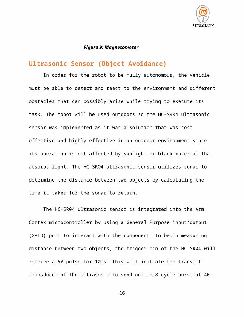
Ultrasonic Sensor (Object Avoidance)In order for the robot to be fully autonomous, the vehicle must be able to detect and react

to the environment and different obstacles that can possibly arise while trying to execute its task.

The robot will be used outdoors so the HC-SR04 ultrasonic sensor was implemented as it was a

solution that was cost effective and highly effective in an outdoor environment since its

operation is not affected by sunlight or black material that absorbs light. The HC-SRO4

ultrasonic sensor utilizes sonar to determine the distance between two objects by calculating the

time it takes for the sonar to return.

The HC-SR04 ultrasonic sensor is integrated into the Arm Cortex microcontroller by

using a General Purpose input/output (GPIO) port to interact with the component. To begin

measuring distance between two objects, the trigger pin of the HC-SR04 will receive a 5V pulse

for 10us. This will initiate the transmit transducer of the ultrasonic to send out an 8 cycle burst at

40 kHz (See Figure 10). As this process is occurring, an interrupt timer will begin counting the

10

Figure 9: Magnetometer Calibration

time until the reflected ultrasonic signal is sensed by the receiver of the ultrasonic. The time is

then multiplied by the speed of sound (C = 340 m/s) and divided by two in order to realize the

distance from two objects going in one direction. If there is reflected signal sensed, the output

pin will give a 38ms high level signal.

If a reflected burst signal is sensed (See Figure 11), the Arm Cortex will send a pulse

width to the steering servo of the robot to turn maximum left in order to avoid the object. Then

the heading will be recalculated and the robot will continue to its destination.

11

Figure 10: Timing Diagram

Figure 11: Trigger Pulse (Yellow), Echo Pulse (Green)

NavigationOnce we figured out what kind of Magnetometer and GPS module to use, then the next

step was to integrate them together in order for our vehicle to be able to fully autonomously

navigate. The other key components into navigation would be the Servo for steering and the

Electronic Speed Controller known as ESC to control the speed and direction of the motor.

The very first thing we did for navigation was to figure out how to use the micro-

controller to control the ESC in order to change speed and direction of the motor. Using the

already included library known as Servo.h, controlling the motor was very simple. In order to

control the ESC there are three inputs that one must know. There is a white wire, which is known

as the signal, the other two are the 5V power and ground. The signal wire must be connected to

one of the dedicated PWM pins on the Arduino Due. The same thing is done with the Servo

where we chose to connect the ESC to pin 9 and the Servo to pin 10.

We found the characteristics of our chassis in order to understand what pulse widths we

needed to send to the ESC or Servo to do certain things. We first figured out what kind of pulse

width we needed to send to the ESC so that the vehicle would move at roughly 10mph on grass.

The next thing we did was to figure out how far the steering Servo could turn to the right and to

the left. We figured that the steering Servo would only be able to turn to the left or right a

maximum of 45°.

12

Figure 12: Pulse Widths and Servo Motor

Once we figured out the characteristics of the steering Servo angle and the speed our

vehicle would be moving on grass, we needed to figure out a method that would move our

vehicle to the waypoints. Since we know the latitude and longitude of the waypoint and current

vehicle we can use Pythagorean’s theorem, which would calculate the distance. The next thing

we needed to know was the heading the vehicle needed to be in, in order to travel in the correct

direction. This was found by using:

θ=tan−1( oppositeadjacent )

In order to increase the accuracy of our navigation, we will the power of our ARM-Cortex to be

constantly updating the distance and heading until we have reached within a certain threshold of

the waypoint.

The magnetometer comes into play by checking constantly if the vehicle’s heading

matches the calculated heading from the waypoint. If the heading does not match the

magnetometer’s heading, our vehicle will steer left or right in order to correct itself. If the

13

Figure 13: Distance Formula

heading of the magnetometer and the calculated heading match, we would make the steering

Servo stay straight and only correct itself if they do not match.

We ran into a few problems when we were using this method of navigation to move our

vehicle to a waypoint. Our vehicle was moving too fast to the waypoint and sometimes it would

continuously drive circles around the waypoint and never actually get to the waypoint. We

decided that the best solution is to slow the speed of the vehicle once it gets closer to the

waypoint. The speed would decrease after 5 meters away from the waypoint and increase the

steering Servo angle in order to make more sharp turns. This added feature has definitely

improved the accuracy of the vehicle actually reaching the waypoint.

14

Figure 14: Navigation Algorithm

Electromagnetic DetectionFor this project, the IED was simulated using an electromagnetic 80 KHz sinusoidal AM

signal propagating from a loop antenna. As a team we were assigned the task of designing,

building, testing and implementing an EM detection mechanism to be integrated into our vehicle.

We decided to go with a simple design to immediately drop the payload once a threshold voltage

occurred from the ADC in the microcontroller.

To accomplish our task, we first had to build our own antenna to pick up the signal form

the loop antenna. We decided to use a two inch ferrite iron core wrapped with a 32 gauge copper

wire as our antenna. This made it small enough to be easily mounted onto our vehicle while

getting sufficient windings for decent inductance. The loop stick antenna had to be perfectly

tuned to pick up the 80 KHz signal thus after we measured the inductance, we used the equation

fc= 12π √ LC

to calculate the capacitance. After much testing I noticed this formula only got me

relatively close for tuning and the capacitance had to be experimentally calculated. Over the

course of this project we ended up building four different loop stick antennas with different

inductances and thus different capacitances. The antenna is shown in the figure below.

15

R 4

1 0 k

R 5

1 0 0 k

0

0

-9 V d c

9 V d c

0

C 2

1 0 u F

-

+

U 2 A

M C 3 3 0 7 8

3

21

84

The next step of the EM

detection integration was the circuit design. Much of the difficultly of building the circuit was

the clutter of information on the internet and its complexity. We wanted the amplitude of the

sinusoidal signal to associate with the distance from the beacon. Also, due to the difficulty of

eliminating noise radiating from the other components on the vehicle, the EM circuit ran on its

own power supply of two 9V batteries. The final circuit consisted of four stages: the tuned loop

stick antenna (antenna circuit), the gain stage, the rectifier stage, and the RC circuit stage

(Appendix E).

The gain stage came to be a non-inverting amplifier. The gain stage came to be

particularly picky because too much gain and the signal rails too quickly but too little gain and

the vehicle has to be right on top of the beacon to be able to pick it up. We wanted to detect the

80 KHz signal from a reasonable distance with greater accuracy than the GPS. With our selection

of the RC car and its turning arc, we decided that four feet was a good distance. After some

experimentation, a gain of eleven gave our desired results. A low pass filter was also added into

the gain stage to filter out the high frequency component of the motor of our vehicle. Of course,

the op amp was selected so significant gain was achievable at the desired frequency of 80 KHz.

The gain stage is shown in the figure below.

16

Figure 15: Ferrite Rod Antenna and PCB

R 4

1 0 k

R 5

1 0 0 k

0

0

-9 V d c

9 V d c

0

C 2

1 0 u F

-

+

U 2 A

M C 3 3 0 7 8

3

21

84

After the gain stage, came the rectification stage which

was set to an inverting unity gain half wave precision rectifier. This topology inverts the negative

cycle while making the positive cycle zero.

This configuration also allowed us to detect

voltages lower than the forward voltage drop

associated from the diodes at the output.

However, the op amp had to have a relatively

fast slew rate as well as a good gain-bandwidth

product at 80 kHz. The rectification stage is

shown in the figure to the right.

The final stage of the EM detection circuit was the RC circuit. This part of the circuit

takes our rectified signal and makes it mostly DC to go into our microcontrollers ADC. The RC

circuit had to hold the voltage long enough for the microcontroller to read it accurately. After

some testing, we found 2 sec to be significantly enough and using the formula 1

RC =τ we

calculated the needed values for the resistor and the capacitor. Subsequently the microcontroller

17

++

-

O P A 2 2 8U 1

D bre a k

D 1

D b re ak

D 2

R 1

1 0 k

R 2

1 0 k

0

0

0

-9 V d c

9V d c

Figure 16: Gain Stage

Figure 17: Rectification Stage

C 11 u

R 35 0 0 k

00

D I O D E Z E N E R

0

M ic ro c o n t ro lle rR 6

2 0 0

can only handle 3.3V maximum, thus a shunt 3.3V zener diode was add to protect the pin of the

microcontroller. The RC circuit is shown in the figure below.

Payload SystemSince we wanted to put the payload on the bottom of the vehicle, we needed a design

made for the low clearance. The design of the payload was made in Solidworks because we

could easily obtain these specific dimensions. The payload pipe is 5.5 inches long with a 2 inch

diameter and 3 degrees incline wedge mounted on top. The wedge allows the pipe to be mounted

at the bottom with a decline slope. This slope allows gravity to take force and drop the golf balls.

The horn rod is 5.25 in long with 1.5 inch rods. The horn rods are at a 22 degree difference. The

horn rod will be connected to HS-645MG standard servo motor. We chose this servo motor

because it had metal gears and has high torque capability. The torque and metal gears are

important because we want it to be capable of holding the weights of the balls. If we rotate the

rod at 22 degrees once, the first ball will drop. At 44 degrees ball two and at 66 degrees ball three

will drop. In figure 19 you can see the rotation.

18

Figure 18: RC Circuit

Figure 19: Payload System Figure 20: Attached Payload Mechanism

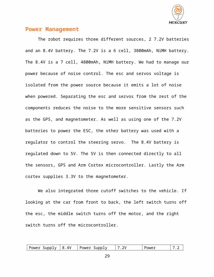
Power ManagementThe robot requires three different sources, 2 7.2V batteries and an 8.4V battery. The 7.2V

is a 6 cell, 3800mAh, NiMH battery. The 8.4V is a 7 cell, 4800mAh, NiMH battery. We had to

manage our power because of noise control. The esc and servos voltage is isolated from the

power source because it emits a lot of noise when powered. Separating the esc and servos from

the rest of the components reduces the noise to the more sensitive sensors such as the GPS, and

magnetometer. As well as using one of the 7.2V batteries to power the ESC, the other battery

was used with a regulator to control the steering servo. The 8.4V battery is regulated down to

5V. The 5V is then connected directly to all the sensors, GPS and Arm Cortex microcontroller.

Lastly the Arm cortex supplies 3.3V to the magnetometer.

We also integrated three cutoff switches to the vehicle. If looking at the car from front to

back, the left switch turns off the esc, the middle switch turns off the motor, and the right switch

turns off the microcontroller.

Power Supply 8.4V Power Supply 7.2V Power Supply 7.2VArm Cortex 8.4V Brushed Motor/ESC UP TO 7.2V Regulator 5VUltrasonic Sensor 5V Steering Servo 5VDrop Servo Motor 5VMagnetometer 3.3VRegulator 5V

From the table above you can see that powering each of the servo motors separately was

important. This is the reason we have three batteries.

19

ConclusionAs we progressed in the design and development of the autonomous robot, many issues

arose that had to be corrected; properly laying out components and modules made a tremendous

difference in our final design. This contributed to our overall system working properly. When

dealing with electronics, there are two types of interference that must be considered, insulated

interference and radiated interference. The insulted interference came directly from the ground of

our power supply which was made noisy by hardware components and PCB’s. This included

voltage regulators and amplifying circuitry. Another key factor that affected our system from

properly working was electromagnetic interference which was caused from the brushed motor

and the servo motors that were used for locomotion, steering, and the payload. Since these

motors are controlled by switching power on or off, electromagnetic fields are created and these

fields must be contained to not interfere with the other components. The main problem was

integrating all the sensors, modules, and components together to create a system that will work

together to complete a task. Properly scheduling and data rates must be considered so that each

sensor and module is able to execute its assignment without interfering or delaying with other

tasks that must be also completed. All these issues allowed us to use concepts and theories of

electrical and computer engineering to create a solution.

In conclusion, real world engineering problems arose and had to be solved using proper

strategies which were implemented to come up with a solution. Each phase was executed and the

expected outcome was obtained. Even though success was reached, many things could have been

approached differently to make the project smoother. The risk of damaging components, sensors,

or PCBs is high. Having multiple spare parts is key to meeting deadlines and completing the

overall project on time, but this is an experience that will be remembered and will help us in the

20

future. Many experiences were obtained and the theories and concepts learned through education

came to life. At the end of the semester, Project Mercury and its autonomous vehicle came out

victorious.

21

Appendices

Appendix A: Mock-Up Illustration

22

Appendix B: Milestones

23

Appendix C: Budget

24

300

14080

200

Cost Analysis

LocomotionSensorsUtilityMisc

$750 Budget Allocation

Budget Pie Chart

Appendix D: PCB Designs

Main PCB Design

1. LM7805 REGULATOR

2. GPS

3. Ultrasonic(s)

4. Antenna(s)

5. Magnetometer

6. Servo Motors

Antenna PCB Design25

Regulator PCB Design

Appendix E: Schematics

26

Complete Antenna Circuit

27

Appendix F: Code Segments

/* static */double distanceBetween(double lat1, double long1, double lat2, double long2){ // returns distance in meters between two positions, both specified // as signed decimal-degrees latitude and longitude. Uses great-circle // distance computation for hypothetical sphere of radius 6372795 meters. // Because Earth is no exact sphere double delta = radians(long1-long2); double sdlong = sin(delta); double cdlong = cos(delta); lat1 = radians(lat1); lat2 = radians(lat2); double slat1 = sin(lat1); double clat1 = cos(lat1); double slat2 = sin(lat2); double clat2 = cos(lat2); delta = (clat1 * slat2) - (slat1 * clat2 * cdlong); delta = sq(delta); delta += sq(clat2 * sdlong); delta = sqrt(delta); double denom = (slat1 * slat2) + (clat1 * clat2 * cdlong); delta = atan2(delta, denom); return delta * 6372795;}

//send string to GPSvoid sendCommand(char *str) { Serial1.println(str);}

double courseTo(double lat1, double long1, double lat2, double long2){ // returns course in degrees (North=0, West=270) from position 1 to position 2, // both specified as signed decimal-degrees latitude and longitude. // Because Earth is no exact sphere, calculated course may be off by a tiny fraction. double dlon = radians(long2-long1); lat1 = radians(lat1); lat2 = radians(lat2); double a1 = sin(dlon) * cos(lat2); double a2 = sin(lat1) * cos(lat2) * cos(dlon); a2 = cos(lat1) * sin(lat2) - a2; a2 = atan2(a1, a2); if (a2 < 0.0) { a2 += TWO_PI; } return degrees(a2);}

bool TinyGPSPlus::encode(char c){

28

++encodedCharCount;

switch(c) { case ',': // term terminators parity ^= (uint8_t)c; case '\r': case '\n': case '*': { bool isValidSentence = false; if (curTermOffset < sizeof(term)) { term[curTermOffset] = 0; isValidSentence = endOfTermHandler(); } ++curTermNumber; curTermOffset = 0; isChecksumTerm = c == '*'; return isValidSentence; } break;

case '$': // sentence begin curTermNumber = curTermOffset = 0; parity = 0; curSentenceType = GPS_SENTENCE_OTHER; isChecksumTerm = false; sentenceHasFix = false; return false;

default: // ordinary characters if (curTermOffset < sizeof(term) - 1) term[curTermOffset++] = c; if (!isChecksumTerm) parity ^= c; return false; } return false;}

29