vinothsv.files.wordpress.com€¦ · web view · 2018-03-19calculate change in net working...

1

Unit I – Introduction to Financial Modelling

1.1 Financial Modelling - Definition

Financial modeling is the task of building an abstract representation (a model) of a real world financial situation. This is a mathematical model designed to represent (a simplified version of) the performance of a financial asset or portfolio of a business, project, or any other investment. Financial modeling is a general term that means different things to different users; the reference usually relates either to accounting and corporate finance applications, or to quantitative finance applications.

1.2 Applications of Financial Modeling

The key Applications of Financial Modeling are Business valuation Scenario planning Capital budgeting Financial statement analysis Project finance Risk Management Portfolio Evaluation Data Representation

1.3 Features of a Financial Model

Unlike simple spreadsheets, a financial model is much more1. It is structured–with a logical flow of assumptions, inputs, calculations and outputs2. It is Dynamic, thus allows the user to change inputs and observe what happens to outputs. This allows for sensitivity analysis.3. It is more Readable as compared to a general spreadsheet 4. It allows for Error Handling5. It should have an objective

1.4 Importance in Financial Model

Remember, in today’s world, collaboration is very important. Multiple people work on the same project. Therefore, it is important for Financial Models to be1. Accurate and Reliable2. Flexible3. User Friendly

Advanced Financial Modelling

2

1.5 Major Do’s and Don’ts in Financial Modelling

For a financial model, some major things to be taken care of are

All items should be in the same font – unless something is a header that needs to attract attention

Decimal points should be same across the entire model Units should be displayed prominently – INR, Million, Nos., % Model objectives should be clearly defined Model inputs, assumptions should be clearly defined Model flow should be clearly defined.

1.6 Defining Model Objectives

It is important to define model objectives first, before embarking upon creating a financial model. Why are we building this model?

Is it for comparing financials? Is it to look at asset allocation? Is it to do risk analysis? Is it to find out some repayment schedule?

1.7 Process Flow for a Model

Assume we are building a valuation model for a company that runs cinema screens, like PVR or Inox. Let us lay down the objectives, inputs, model flow and outputs expected.

Objective – Valuation of Equity (Method: Discounted Cash Flow/Relative Valuation)

InputsCash Flow P & L A/c, Balance

Sheet Revenues, Costs and others

Cost of Capital Rf, Beta, Rm-Rf, Wd, We, Cd and Tax rate

Revenue Estimation – Ticket – Ave.Ticket Price x Seats x Occupancy x Screens x Shows x 365 +

Food & Beverage – People Visiting x % of Eating x Ave. Spend +

Advt – Advt/ Scree + Parking etc.

Process

Revenues Assumptions: P&L, BS, CF, Debt Schedule, Capex Schedule, DCF

Less: Costs Profits -- Cash Flow -- Discount


3

Output: Result

1.8 Identifying Inputs and Variables

We need to define the key values we will need in any model to be able to arrive at the final conclusion. We have already seen examples of this. For example, while doing valuation, we need to identify what are the key inputs and assumptions in our model. How are we projecting those? We also need to mention these, or show them in a different color, so as to make sure that everyone understands what an assumption is, and what data that is given is.

Defining DeliverablesThe Model Output has to be defined, so that we are clear about what is it that we can expect, and where can we find it. May be it could also be shown in a different color, and the model introduction should mention what we are trying to find?

Stress TestingWhen a model has many inputs, they may start affecting the overall flow. It is therefore important to see if changes to one input are not affecting any other functionality anywhere. A model has to be stress tested to see if all linkages are working correctly, or not.

1.9 DocumentationA financial Model is in complete without some documentation about how the model flow moves. Documentation can be done in 3ways1. Using Name Manager – Define Names for the Inputs such that understanding the model becomes easier.2. Using In Cell Comments –Defining comments for any assumption, so that a user can understand why those assumptions have been made.3. Using separate columns for comments, or using an entire sheet for documenting the key assumptions and Model Flow.A combination of the above can also be used.

********


4

Unit II – Portfolio and Options Modelling

2.1 Variance Covariance

Calculating Daily returns for DLF, Eicher & Hindalco:a. In Cell E8 – use the formula = (Today Value – Yesterday Value) / Yesterday Value for

calculating Daily returns – Convert into % and drag to right and down for the entire period

Calculating Daily & Annual Average returns and Standard Deviationsa. In Cell E502, calculate Daily average returns =AVERAGE(E8:E500) and drag it up to

H502b. In Cell E503, calculate Annual returns =(1+E502)^250-1 and drag it up to H503c. In Cell E504, calculate Daily Standard Deviation =STDEV.P(E8:E500) and drag it up to

H504d. In Cell E505, calculate Annual Standard Deviation =E504*SQRT(250) and drag it up to

H505.e. In Cell E506, calculate Daily Variance =E504*E504 and drag it up to H506


5

Calculating Variance and SD for Two Asset Portfolio

If there is a portfolio with 2 assets, we already know the returns and standard deviation of this portfolio. Returns are weighted average, while portfolio variance is given by the following formulaPortfolio Variance = w2A*σ2(RA) + w2B*σ2(RB) + 2*(wA)*(wB)*Cov(RA, RB)

a. Take 2 asset out of the portfolio DLF and Eicher and assume you’re investing 40% with DLF and 60% with Eicher.

b. In CellE510 calculate Portfolio average returns =B508*E503+B509*F503c. Calculate Covariance in Cell E513, F513, E514 and F514.

i. For E513 =COVAR(E8:E500,E8:E500)ii. For F513 =COVAR(E8:E500,F8:F500)

iii. For E514 =COVAR(F8:F500,E8:E500)iv. For F514 =COVAR(F8:F500,F8:F500)

d. Calculate Variance in Cell E517, E517, E518, F518.i. For E517 =E511*C513*E513

ii. For F517 =F511*C513*F513iii. For E518 =C514*E511*E514iv. For F518 =F511*C514*F514

e. Calculate Variance in Cell B517 =SUM(E517:F518) and SD in cell B518 =SQRT(B517)

Portfolio Variance for Three Asset Portfolio

Returns are still weighted average, while portfolio variance is given by the following formula

Portfolio Variance = w2A*σ2(RA) + w2B*σ2(RB) + w2C*σ2(RC) + 2*(wA)*(wB)*Cov(RA, RB) + 2*(wA)*(wC)*Cov(RA, RC) + 2*(wB)*(wC)*Cov(RB, RC)

Assume a portfolio with 3 assets. The weights are 20% for DLF, 35% for Eicher and 45% for Hindalco respectively. Below are the details of Standard Deviations and Correlations.


6

a. Calculate Covariance between DLF,Eicher and Hindalco i. For Cell E529 =COVARIANCE.P(E8:E500,E8:E500)

ii. For Cell F529 =COVARIANCE.P(E8:E500,F8:F500)iii. For Cell G529 =COVARIANCE.P(E8:E500,G8:G500)iv. For Cell E530 =COVARIANCE.P(F8:F500,E8:E500)v. For Cell F530 =COVARIANCE.P(F8:F500,F8:F500)

vi. For Cell G530 =COVARIANCE.P(F8:F500,G8:G500)vii. For Cell E531 =COVARIANCE.P(G8:G500,E8:E500)

viii. For Cell F531 =COVARIANCE.P(G8:G500,F8:F500)ix. For Cell G531 =COVARIANCE.P(G8:G500,G8:G500)

b. Calculate Variance between DLF, Eicher and Hindalcoi. For Cell E534 =$C529*E$527*E529

ii. For Cell F534 =$C529*F$527*F529iii. For Cell G534 =$C529*G$527*G529iv. For Cell E535 =$C530*E$527*E530v. For Cell F535 =$C530*F$527*F530

vi. For Cell G535 =$C530*G$527*G530vii. For Cell E536 =$C531*E$527*E531

viii. For Cell F536 =$C531*F$527*F531ix. For Cell G536 =$C531*G$527*G531

c. Calculate Portfolio Variance in Cell B534 =SUM(E534:G536)d. Calculate Portfolio SD in Cell B535 =SQRT(B534)

Using Solvera. Go to File – Options – Add Ins and Click Go to insert Solver in to your data tab.b. Go to Data Tab – Select Solver – Set objective with Cell K532 (Average of Returns) then

click Minc. Select changing variables as Weights Cells J528:J530d. Add Constraints – J528, J529 and J530 are >= 5%


7

e. Add Constraint – J531 = 100%f. Add Constraint with K532 is >=30% and K536 is <=10% then Click Solve.g. Let you can able to see the changes in the weights as output.

2.2 Portfolio

Normal DistributionIn Finance, returns are expected to be distributed normally. Let us understand the normal distribution first.


8

Assume a stock with expected return 15%, and standard deviation of 20%. How would the normal curve look like?

a. Type Mean value and SD value in Cell B4 and B5b. Calculate Normal Distribution in Cells B10: B13 for Probability of returns less than 15%,

-5%.-25% and 35%; =NORM.DIST(A10,$B$4,$B$5,1)c. Calculate Normal inverse for Probability of returns less than 15%, -5%.-25% and 35%;

=NORM.INV(B10,$B$4,$B$5)d. Present inverse values in G4:G7 for presentation.

2.3 Simulation – Monto Carlo Simulation

Sometimes, we may need to run a simulation to find out if the results that are expected are feasible or not.Take for example an investment product, that says that if you invest Rs100,000 today in an asset with mean of 20% and SD of 18%, you will be given 10lakhs, if the total investment value crosses 8 lakhs at the end of 10years, else you will be given Rs3 lakhs.

a. Type mean value and SD value in Cell B4 and B5b. Type year 1 to 10 from E5:E14 and enter investment value as Rs.1,00,000 in Cell F4c. Calculate Return % in Cell G5; =NORM.INV(RAND(),$B$4,$B$5)d. Calculate returns in F5; =F4*(1+G5) and drag return and rate up to 14th row.e. In cell B11 link the 10th return value = 509,466f. For simulation and 1000 iteration enter number 1 to 1000 from cell A12 to A1011g. To get simulated return, Select A11:B1011 go to Data tab -> Select What-if-Analysis –

Select – Data Table, keep empty the row input cell and column input select cell C11. You will get the data filled up to 1000 iterations

h. Calculate Average Ending Value in Cell B7 =AVERAGE(B12:B1011)i. Calculate Annualized return in Cell B8 by using CAGR formula =(B7/F4)^(1/10)-1


9

2.4 Option Payoff

Options – MeaningOptions are a kind of derivative instruments, where the holder of the option has a right but no obligation to buy or sell an asset. Unlike futures – where the buyer and the seller of the future enter into a contract for executing a transaction on a set date at a set price – the option, as the name signifies, is an option for the holder to decide whether or not he wants to execute the trade.

Option Terminologies: Strike Price/Exercise Price – It is the price at which the option can get exercised, Spot Price – Underlying or current market price Premium – It is the price we pay for the option Option Writer – The entity who sells the option. This entity is said to short the option Option Holder - The entity who buys the option. This entity is said to be Long the option

Type of Options:

Call Option – It is an option that gives the buyer of the option a right to buy the underlying asset at a predetermined price (Strike Price).

Put Option – It is an option that gives the buyer of the option a right to sell the underlying asset at a predetermined price (Strike Price).

Option PayoffsConsider a call option on a stock with an expiry this month. Its details are as mentioned below.Strike Price – Rs.2500; Step – 50, Premium – 25Let us create the payoff matrix for this option

a. Type option type as Call in Cell B4 and Strike Price – Rs.2500; Step – 50, Premium – 25 in cell B5, B6 and B7

b. Create a Payoff Schedule with Underlying Price, Profit/Loss, Premium paid, Total Buyer Payoff, Total Seller Payoff from A9 to E9

c. Enter 2500 in Cell A15 and reduce the value by 50 to the above 5 cells and increase the value of 50 by below 5 cells.


10

d. Enter Premium paid as -25 commonly from Cell C10 to C20e. Use nested IF formula for calculating Profit/Loss =IF($B$4="Call",IF(A10>$B$5,A10-

$B$5,0),IF(A10>$B$5,0,$B$5-A10)) f. Calculate Total Buyer Payoff in Cell D10 =B10+C10 drag up to D20g. Calculate Total Seller Payoff in Cell E10 =-D10 drag up to E20h. Select Underlying Price A10:A20, Total Buyer Payoff D10:D20 and Total Seller Payoff

E10:E20 go to Insert Tab and Insert Line Chart for Presentation.

2.5 Cash Future ConvergenceConvergence is the movement of the price of a futures contract towards the spot price of the underlying cash commodity as the delivery date approaches.

a. Take Future Price & Spot Price from NSEINDIA.Com

b. In Cell B7 type expiry date and in Cell B8 type date from NSE Sitec. Calculate days to expiry in Cell B3 =B7-B8


11

d. Calculate daily implied interest rate in B6 =((B4/B5)^(1/B3)-1) and annual rate in C6 =B6*365

e. Assume Annual Mean is 15% and SD is 18% in Cell F4 & F5f. Calculate Daily Mean in Cell E4 =(1+F4)^(1/250)-1 and In Cell E5 calculate daily SD

=F5/SQRT(250)g. The headers in 10th row Days to Expiry, Future Price, Spot Price, Spot Return h. In 11th row link Days to expiry from B3, Future Price from B4 and Spot Price from B5i. Calculate Spot return in Cell D12 =NORM.INV(RAND(),$E$4,$E$5)j. Calculate Spot Price in Cell C12 =C11*(1+D12)k. Calculate Future Price in Cell B12 =C12*(1+$B$6)^A12l. Select from B12 to D12 drag down to 0 Expiry daysm. Select Days to Expiry, Future Price and Spot price - A10:D45 Go to Insert Tab and Insert

line chart for presentation.


12

Unit III - Financial Modeling for Valuation and FSA

3.1 Forecasting Revenues and Costs

Objective: Forecast revenue and costs for the following data:

2009 2010 2011 2012 2013 2014 2015Year 1 2 3 4 5 6 7Sales 411 488 737 1,174

RM Cost 236 287 459 697 Net Profit 46 86 142 174

Calculate by using any of the following three methods:1. Historical Average2. Trend Analysis - Linear Regression3. Proportion - Cost as % of sales

Method 1: Historical Average

a. Copy the data from sales to Net Profit completely and paste to the CELL down (A12:E14)

b. Go Cell C12 Calculate Growth using the formula = (Current Value – Previous Value)/ Previous Value - > =(C8-B8)/B8. Keep Blank the B12 cell.

c. Copy/Drag the formula for rest of the cells. d. Calculate Average for 3 years growth rate = AVERAGE (C12:E12), Similar for the two

items.e. Go To -> Cell No. F8 and Calculate forecast Value = Previous Cell Value (E8) * 1+

Growth rate (1+F12)) and drag the same for two more years.Follow the same instruction for RM Cost and Profit forecast.


13

Method 2: Trend Analysis - Linear Regression.a. Select the 3 items data for 4 years -> B8: E10 -> Go to Insert -> Line Chart -> Right in

side chart add Trend Line (Linear) and Click Display Equation on the chart - > The Equation appears like this: y = 253.74x + 68.265

b. Go to Cell F8, Calculate forecast value like this (253.74 *5) + 68.265; similarly for other cells by using manual formula.

c. Second method of Forecasting is called as “FORECAST”d. Go To Cell F8 =FORECAST(x, known_y's,known_x's); Use following inputs for getting

forecast values- X = 5 (5th Year), known_y’s (Sales amount from 2009 to 2012 – $B$8:E8),

known_x’s (Year 1 to 4; $B$7:E7). Use same FORECAST function for remaining cells.


14

Method 3: Proportion - Cost as % of sales

a. Go To Cell B12 and Calculate Cost as % of Sales by using the formula = RM Cost (B8) / Sales (B7) and drag the same up to E12.

b. Calculate 4 years values as forecast = Average (B12:E12) and drag the same up to H12.

3.2 Financial Statement Analysis and Projection


15

Revenue Drivers:a. For calculating revenue per car -> Use Assumption sheet -> The Values: Installed

Capacity, Car Sales are already given in the Assumption sheet for the year Financial Year 11 to 15.

b. Link and bring the Revenue from operations Value from Profit and Loss Account -> = ='P&L'!B6 (Gross Revenue from Operations)

c. Calculate Price per Car = Revenue from Operations / Car Sales – Total; =(C14*10^7)/C12. We are using *10^7 for converting value from Million to Crores.

d. Drag both Cell C14 & C15 to G14 & G15.e. Assume the Number of Sales is Same – 1292415 and Price per car is Rs.400,000. f. Calculate Revenue from Operations for FY16 = Rs.400,000 * 1,292,415 ( H15 * H12 /

10^7).

Cost Driversa. Calculate Cost drivers from row 20 onwards.b. Calculating Cost of Material: calculate based on Price per Car -> Go To cell C21 -> Cost

of Material *10 ^7 /Total Car Sales; =(C20*10^7)/C12 drag the same up to G21. Calculate average 3 years as Forecasted Cost of Material per car for FY16; =AVERAGE(E21:G21)

c. Cost of Material for FY16 -> Total Car Sales for FY16 * Average Cost of Material per Car; =H12*H21/10^7

d. Calculating other costs like Purchases of Stock-in-trade, Change in Inventories, Employees Benefits Expenses, other expenses and vehicles/dies for own use are based on % of Sales.

e. Calculation as % of sales – Particular Expenses / Revenue from operations. = =C22/C$14f. Calculation of Expenses is Average for 3 years of % of sales * Revenue from operations.

= H23*$H$14

Working Capital Drivers


16

a. All the working capital items are calculated based on % of Sales.b. Calculation of % of Sales for Working Capital items – Select working capital item value /

Sales present as %

c. Example: Short term Borrowing amount (C40) / Revenue from operations; =C40/C$14. For FY16 take the average of three months (Example for Short Term Borrowings is 1.5%). Do the same for others.

d. Calculating in terms of days’ worth of sales= Percentage of Working Capital item * 365 days. Example for Short term Borrowing =C52*365

Forecasting Working Capital Drivers for FY16a. Working Capital item value for FY16 = % of Sales of particular item * Revenue from

operations.b. Example for Short Term Borrowings FY16 = Revenue from Operations (H14) * % of

Sales of Short Term Borrowing (H52); =H52*H$14.


17

Profit and Loss Account Forecasting/Projectiona. Link revenue from operations value for FY16 from Assumption sheet =Assumptions!H14b. Use previous year(FY15) values of Excise duty, Other operating income and other

income as same for current year(FY16) too.c. For calculating Total Operating Revenue- use the formula Netsales + Other Operating

Revenue; =G8+G9.d. Link the expenses from Assumption Sheet. =Assumptions!H20, =Assumptions!H22,

=Assumptions!H24, =Assumptions!H26, =Assumptions!H28, =Assumptions!H30.e. Calculate sum value as Total Operating Expensesf. For EBIDTA (G24) = Total Operating Revenue (G12) – Total Operating Expenses

(G22).g. EBIDTA Margins = EBITDA / Net Sales. Example for FY11 = =B24/B8. Drag up to

FY16.h. Use Same amount of Depreciation and Finance Cost from FY15 to FY16i. Calculating Tax rate = Tax amount / EBT drag up to FY15. Use FY15 percentage for

FY16. Tax amount for FY16 = Tax rate * EBT for FY16.j. PAT or Net Profit = EBT – Tax


18

CAPEX Schedule:a. Go To Capex Schedule worksheet -> Calculate Gross LT Assets per car Capacity ->

Total Gross Long Term Assets *10^7/Capacity -> =B6*10^7/B10; drag upto FY14.b. Forecasting for FY15 use the same value from FY14.c. Forecasting for FY16 = Link FY15 value of Capacity + 5000 increasing and Gross LT

Assets per capacity become same.d. Calculating Capex = (Capacity FY16 – Capacity FY15) * Gross LT Assets per Car /

10^7; =(G10-F10)*G12/10^7e. Calculating Debt – Assume Debt/Equity ratio is 1:2; = Capex * 1/3; =G14*33%

Balance Sheet Projection

a. Liabilities Projection is the first partb. Share Capital keep same value appearing the FY15c. Reserves & Surplus – FY15 value + PAT or Net Profit of FY16 from P & L

Worksheet; =F9+'P&L'!G37d. Long term Borrowing – FY15 Value + Debt amount from Capex Schedule; =F13+'Capex

Schedule'!G15.


19

e. Remaining Non-current liabilities values take same from FY15 for FY16.

f. All Current Liabilities value link and take from Assumption Sheet. It is already calculated there. =Assumptions!H40, =Assumptions!H41, =Assumptions!H42, =Assumptions!H43

g. Calculate Total Liabilities = Total Shareholder’s Funds + Total Non-Current Liabilities + Total Current Liabilities; =G10+G17+G24

h. Assets classified into two parts Non-Current Assets and Current Assetsi. Total Fixed Assets = FY15 Value – Depreciation from P &L for FY16 + Capex amount

from Capex Schedule for FY16. =F34-'P&L'!G27+'Capex Schedule'!G14.j. Three items Non-Current Investments, Long Term Loans and Advances and Other Non-

Current Assets are same. Link and take it from FY15 to FY16


20

k. Current Assets -> Current Investment Same Value from FY15 to FY16l. Link and take Inventories, Trade Receivables, Short Term Loans and Advances and

Other Current Assets from Assumptions Sheet. = =Assumptions!H45, =Assumptions!H46, =Assumptions!H48, =Assumptions!H49.

m. Link and Take the value of Cash and Bank Balances from Cash Flow Statement. ='Cash Flow'!D14.

n. Total Assets = Total Fixed Assets + Non-Current investment + Long Term Loans and Advances + Other Non-Current Assets + Total Current Assets. =G34+G36+G37+G38+G47

o. Calculate Balance between Total Assets and Total Liabilities = Total Assets (B49) – Total Liabilities (B26).

p. Calculate Change in Net Working Capital for Cash Flow Statement - > Take Non Cash Current Assets (Excluding Current Investments & Cash and Bank Balances) - > =B42+B43+B45+B46. Link and take Current Liabilities from Cell =B24

q. Calculate Net Working Capital = Non Cash Current Assets – Current Liabilities; =B54-B55

r. Calculate Change in Net Working Capital = Current Year Net Working Capital – Previous Year Net Working Capital; =C57-B57 drag up to FY16.

Cash Flow Statement

a. Preparing the Cash Flow Statement, first link the Net Profit from P & L Account; ='P&L'!G37


21

b. Depreciation link and bring from P & L Account; ='P&L'!G27c. Changes in Net Working Capital – link and bring from Balance Sheet Worksheet;

='Balance Sheet'!G58d. Capital Expenditure (CAPEX) – link and bring from Capex Schedule; ='Capex & Debt

Schedule'!G14e. Changes to Debt – link and bring from Capex Schedule - ='Capex & Debt Schedule'!G15f. Calculate Total Cash Flow = Net Profit + Depreciation – Changes in Net Working

Capital – Capital Expenditure + Changes to Debt; =D6+D7-D8-D9+D10g. Link and bring FY15 Cash as opening cash balance for FY16h. Calculate Closing Cash Balance = Total Cash Flow + Opening Cash Balance; =D12+D13i. Link the calculated closing cash balance to Balance Sheet (Cell No. ='Balance Sheet'!

G44) ='Cash Flow'!D14

Ratio Analysis

a. Profitability Ratios calculation: Operating Profit Margin = EBITDA/ Total Operating Revenue; ='P&L'!B24/'P&L'!B12

b. EBIT Margin = EBIT/Total Operating Revenue; ='P&L'!B29/'P&L'!B12c. Net Profit Margin = Net Profit/ Total Operating Revenue; ='P&L'!B37/'P&L'!B12d. Return Rations – Return on Equity = Net profit/Shareholders Funds; ='P&L'!

B37/'Balance Sheet'!B10e. Return on Capital Employed = EBIT / (Shareholder Funds + LT Loans);

='P&L'!B29/('Balance Sheet'!B10+'Balance Sheet'!B13)f. Coverage Ratio - Interest Coverage Ratio = (EBIT / Interest); ='P&L'!B29/'P&L'!B31g. Debt Equity Ratio = Total Debt/Equity; =('Balance Sheet'!B13+'Balance Sheet'!

B20)/'Balance Sheet'!B10h. Solvency/Liquidity Ratios – Current Ratio =Current Assets / Current Liabilities;

='Balance Sheet'!B47/'Balance Sheet'!B24i. Quick Ratio = (Cash + Receivables) / Current Liabilities; =('Balance Sheet'!

B44+'Balance Sheet'!B41+'Balance Sheet'!B43)/'Balance Sheet'!B24


22

j. Turnover Ratios - Inventory Turnover Ratio = Sales / Inventory; ='P&L'!B12/'Balance Sheet'!B42

k. Receivables Turnover Ratio = Sales / Receivables; ='P&L'!B12/'Balance Sheet'!B43l. Total Asset Turnover Ratio = Sales / Total Assets; ='P&L'!B12/'Balance Sheet'!B49m. Fixed Asset Turnover Ratio = Sales / Fixed Assets; ='P&L'!B12/'Balance Sheet'!B34


23

Unit IV - Financial Modeling for Debt and Bonds

4.1 Models for Debt Repayment

Companies that take debt, need to create a schedule to repay it. The repayment has to be modelled in financial models. There can be various ways this debt can be repaid1. The debt could be repaid in equal monthly installments2. The Principal could be repaid in equal amounts over a tenure3. There could be a specific customized schedule for a certain loan4. The loan repayment could be to manage a certain debt service coverage ratio

Method 1: Equal Monthly Installments

a. Based on the following inputs prepare a Debt Repayment Schedule on Equal Installment Method – Principal Rs.150 Crore, Rate – 8%, Period/Tenure – 9 Years.

b. Link and bring beginning principal from Principal – B3 i.e., Rs.150c. Calculate Installment in Cell no B11 by using PMT formula; =PMT(B4,B5,-B3,0) and

link the same amount in to C11 and drag right up to Cell no J11.d. Calculate Interest payment in Cell B10 = Beginning Principal (B8) * Rate (B4);

=$B$4*B8 and drag the same up to cell no J10e. Calculate Principal Repayment in Cell B9 = Installment (B11) – Interest Payment (B10);

=B11-B10 and drag the same up to cell no J9f. Calculate Closing Principal in Cell B12 = Beginning Principal (B8) – Principal

Repayment (B9); =B8-B9 and drag the same up to Cell J12g. Link Closing Balance in Cell B12 with Beginning Principal in Cell C8 and drag the same

up to Cell J8h. Select Principal Repayment and Interest Payment -> Go to -> Insert Tab -> Select 2D

Area Chart for presentation.


24

Method 2: Equal Principal Repayments

a. Based on the following inputs prepare a Debt Repayment Schedule on Equal Principal Repayment Method – Principal Rs.150 Crore, Rate – 8%, Period/Tenure – 9 Years.

b. Link and bring beginning principal from Principal – B3 i.e., Rs.150c. Calculate Equal principal repayment in Cell B8 = 150/9; Principal (B3)/Tenure(B5);

=B3/$B$5. Link the same amount in to C8 and drag the same up to J8.d. Calculate Interest Repayment in cell B9 = Beginning Principal (B7) * Rate (B4). Drag

the formula up to J9e. Calculate Installment in Cell B10 = Principal Repayment + Interest Payment; =B8+B9,

drag the same formula up to J10f. Calculate Closing Principal in Cell B11 = Beginning Principal (B7) – Principal

Repayment (B8); =B7-B8 and drag the same up to Cell J11g. Link Closing Balance in Cell B11 with Beginning Principal in Cell C7 and drag the same

up to Cell J7h. Select Principal Repayment and Interest Payment -> Go to -> Insert Tab -> Select 2D

Area Chart for presentation.


25

Method 3: Custom Repayment Schedule

a. Based on the following inputs prepare a Debt Repayment Schedule on Custom Repayment Schedule Method – Principal Rs.150 Crore, Rate – 8%, Period/Tenure – 9 Years. The bank has asked the repayment for the first 4 years to be 5% each, while the next 5 years to be 16% each.

b. Link and bring beginning principal from Principal – B3 i.e., Rs.150c. Insert new row and name as Custom Payment Schedule. Enter 5% from Cell B11 to E11

and enter 16% from Cell F11 to J11.d. Calculate principal repayment in cell B12 = Beginning Principal (B10) x Custom

payment % (B11). Drag the formula up to cell J12.e. Calculate Interest Repayment in cell B13 = Beginning Principal (B10) * Rate (B5). Drag

the formula up to J13.f. Calculate Installment = Principal Repayment + Interest payment; B12 + B13 and drag the

formula up to J14.g. Calculate Closing Principal in Cell B15 = Beginning Principal (B10) – Principal

Repayment (B12); =B10-B12 and drag the same up to Cell J15h. Link Closing Balance in Cell B15 with Beginning Principal in Cell C10 and drag the

same up to Cell J10.


26

Method 4: Debt Sculpting

Under this method, the company now incorporates how cash flows could define how much money is being repaid. In the earlier methods, whether the company was making money or not, we were creating a repayment schedule. In real life, that may not be practical. So here, we assume that debt payment would depend on how much cash the company has to service this debt. This can be captured by Debt Service Coverage Ratio.

a. Calculate Cash Flow available for Debt Service by using the formula = EBITDA – Tax. Drag the same formula up to cell J12.

b. Link Principal Amount 150 (Cell B4) with B14 in Beginning Principal.c. Calculate Interest Payment in Cell B16 = Beginning Principal (B14)*Rate(B5) drag the

same up to J16d. Calculate Installment in Cell B13 = CFADS (B12) / DSCR (B7) and drag the same up to

J13.e. Calculate Principal Repayment in Cell B15 = Installment – Interest, and drag the same up

to Cell J15f. Calculate Closing Principal in Cell B17 = Beginning Principal (B14) – Principal

Repayment (B15) and drag the same up to Cell J17


27

4.2 Bonds/Fixed Income Securities

Calculating Clean Price and Dirty Price


28

Calculate Full Price and Clean Pricea. Assume a Bond with above information’s and its face value of Rs.100. Calculate full

price and clean priceb. Calculate number of periods to next coupon – Days to next coupon/Days between

coupons; =D11/D12; 104/182 in Cell D13 along with that add 1 in the next cell E13 drag up to G13

c. Fill/Calculate cash flows in Cell D15 – Face Value (Rs.100)*Coupon (10%)/2 – because of semiannual bond drag up to F15 and fill CF + Face Value i.e., 100+5 = 105 in cell G15

d. Calculate Discounted CF in D16 – CF (D15)/(1+Semiannual Yield(D10-4%)^D13 drag the same formula up to G16

e. Calculate Full Price in Cell D18 – sum of Discounted CF(D16:G16)f. Calculate Accrued Interest in Cell D19 – (Days in Since last coupon(C11 – 78)/Days

between Coupon(D12-182))*CF(D15-5)g. Calculate Clean Price in D20 = Full Price(D18)-Accrued Interest(D19)

Calculating Clean Price using Excel Function – Pricea. Type Settlement date as today date in Cell H7, calculate next coupon date - =H7+104,

calculate maturity date - =H9+183+365.b. Calculate Clean Price using Price function = Price(Settlementdate,

Maturitydate,Rate,Yield,Redemption,Frequency,Basis); =PRICE(H7,H8,D8,D9,100,2,1).


29

4.3 Calculation of Duration

Duration is the measure of the price sensitivity to the changes in yield for a bond

Duration of a bond gives us a measure of how much the bond will move for a 100 basis point (1%) movement in yields. An approximate measure can be found by just changing the YTM of a bond slightly and seeing how much difference does the change make to the price. Let us look at an example.Assume a bond with coupon rate of 8%, tenure of 5 years, face value of Rs100 and YTM (expected return) of 7.2%. The current price can be calculated using the NPV formula, or manually on excel.


30

Coupon 8% Years 1 2 3 4 5

Cash Flows

8.0

8.0

8.0

8.0

108.0

Price 103

.26 Discount Rate 7.2%

DCF

7.46

6.96

6.49

6.06 7

6.29

a. Calculate DCF – CF/(1+7.2%)^t; In Cell D8 =D6/((1+$D$7)^D5) drag up to H8b. Calculate Price in B7 = sum of DCF (D8:H8)c. Vo in Cell C13 type 103.26, if Discount rate is 7.1% type against Vdecline i.e. Cell C14 –

103.68, if Discount rate is 7.3% type against Vincrease i.e. in cell C15 - 102.85.d. When Yield decline/Increase by 10 basis points the duration become 4.

Calculating Duration by using MDuration and Duration Functions:

a. Type today date in Cell C3, from Cell D3 = C3 +365 drag up to H3.b. Calculate MDuration in Cell I11 =

MDURATION(Settlementdate,Maturitydate,Coupon,yield,Frequency,Basis); =MDURATION(C3,H3,B5,D7,1,1).

c. Calculate Duration = MDuration value * (1+Discount Rate); =I11*(1+D7)d. Calculate Duration using function cell – I12 =

DURATION(Settlementdate,Maturitydate,Coupon,yield,Frequency,Basis); =DURATION(C3,H3,B5,D7,1,1).

4.4 Calculating Yield and Coupon Functions

a. Type today in settlement dateb. Use COUPDAYS function to find the days in period in Cell B13 =

COUPDAYS(Settlement, Maturity, Frequency, Basis); =COUPDAYS(B4,B8,B9,1)


31

c. To find Days in Coupon Period Over use COUPDAYBS function in Cell B14 = COUPDAYBS(Settlement, Maturity, Frequency, Basis); =COUPDAYS(B4,B8,B9,1)

d. Calculate Accrued Interest in Cell B15 = =B14/B13*(B7/B9*B6)e. Calculate Clean Price in Cell B11 = Current Market Price – Accrued Interestf. Calculate Yield in Cell B10 = =YIELD (B4,B8,B7,B11/10,B6/10,B9,1) – Note Excel

take Face Value only Rs.100. So, Convert that by divide 10)g. To find Days left in the Coupon Period use COUPDAYSNC function in Cell B17 = =

COUPDASNC(Settlement, Maturity, Frequency, Basis); =COUPDAYS(B4,B8,B9,1)h. To find Next Coupon Date use COUPNCD function in Cell B18 = =

COUPNCD(Settlement, Maturity, Frequency, Basis); =COUPDAYS(B4,B8,B9,1)i. To find Number of Coupons left use COUPNUM function in Cell B19 = COUPNUM

(Settlement, Maturity, Frequency, Basis); =COUPDAYS(B4,B8,B9,1)j. To find Previous Coupon Date use COUPPCD function in Cell B20 = COUPPCD

(Settlement, Maturity, Frequency, Basis); =COUPDAYS(B4,B8,B9,1)


32

Unit V – Case Studies

5.1 Case 1 – Investment Benefit Modelling

You are a financial advisor, who wants to explain to a client that early investing has its benefits.

Your client wants to have Rs 5 crore by the time he retires, that is at the age of 60. He is

currently 25 years old, but plans to save money only after he has a salary of greater than 15

lakhs. His current salary is Rs 2.5 lakhs per annum. Assume rate of return to be 12%, and show

the sensitivity of the returns to the entire problem as well.

You want to showcase that early investing can give him huge benefits, in terms of lower amount

to be invested every year if started early.

Steps:

a. Type 15 in Cell B4 assume the age of the investor is 45 so, he have another 15 years of

service to get retirement

b. Enter Retirement Corpus required by the investor as Rs.5 Crore in B5

c. Enter Expected return as 12% in B6

d. Calculate Annual investment needed by using PMT function in Cell B8 =PMT(B6,B4,0,-

B5)

e. Calculate Monthly investment needed by using PMT function in Cell B9

=PMT(B6/12,B4*12,0,-B5)

f. Link monthly investment needed i.e. B9 with E8 and type horizontally the return

percentages like 10%,11%, 12%, 13%, 14% and 15%

g. List the age 50 to 25 between the cell D9:D14 and period gap for retirement from Cell

E9:E14

h. Select the table E8:K14 go to Data Tab – What-if-Analysis –Data table: Row input is

return rate – B6 and Column input is time frame – B4 then click ok


33

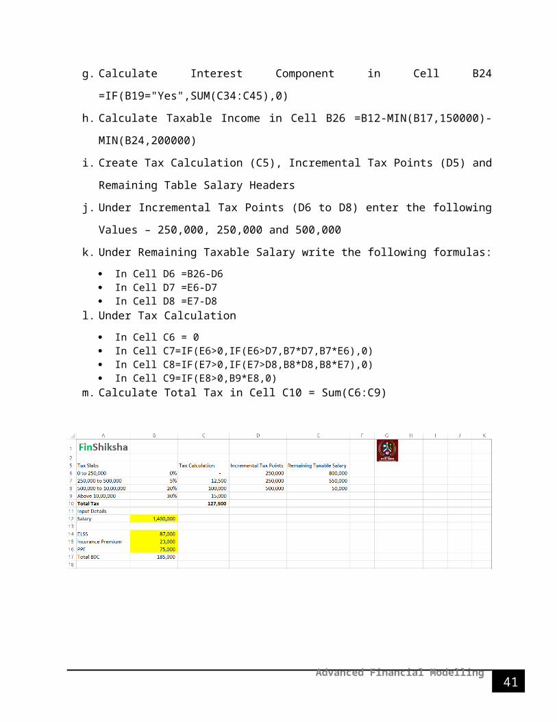
5.2 Case 2 – Income Tax Calculator

You want to create a short tax calculator for Salaried Individuals. You are broadly given the

following data, and will ask the user to input some major parameters about the salary and

investments. Based on this, the taxable income needs to be calculated

Tax Slabs

0 to 250,000 = 0%

250,000 to 500,000 = 5%

500,000 to 10,00,000 = 20%

Above 10,00,000 = 30%

Home Loan Interest Benefit = up to 2 lakhs

Investments in ELSS, Insurance Premium, PPF (80C) = up to 1.5 lakhs

Steps:

a. Enter input details Salary (B12), ELSS(B14), Insurance Premium(B15), PPF(B16)

b. Calculate Total 80C in Cell B17 =SUM(B14:B16)

c. Enter Home Loan taken – Yes/No by using Drop down menu – Data Validation – List –

Select H19&H20 Click ok

d. Enter Interest Rate (B20), Tenure(B21) and Home Loan Amount(B22)

e. Create EMI Schedule A33 to D45 with following headers month, emi, interest, principal

f. Calculate EMI in Cell B34 =PMT(B20/12,B21*12,-B22,0) link with B35 and drag up to

B45; Calculate Interest in Cell C34 – EMI – Principal link the formula in C35 drag up to

C45; Calculate Principal by using PPMT formula in D34


34

=PPMT($B$20/12,A34,$B$21*12,-$B$22,0) link the formula with D35 and drag up to

D45

g. Calculate Interest Component in Cell B24 =IF(B19="Yes",SUM(C34:C45),0)

h. Calculate Taxable Income in Cell B26 =B12-MIN(B17,150000)-MIN(B24,200000)

i. Create Tax Calculation (C5), Incremental Tax Points (D5) and Remaining Table Salary

Headers

j. Under Incremental Tax Points (D6 to D8) enter the following Values – 250,000, 250,000

and 500,000

k. Under Remaining Taxable Salary write the following formulas:

In Cell D6 =B26-D6 In Cell D7 =E6-D7 In Cell D8 =E7-D8

l. Under Tax Calculation

In Cell C6 = 0 In Cell C7=IF(E6>0,IF(E6>D7,B7*D7,B7*E6),0) In Cell C8=IF(E7>0,IF(E7>D8,B8*D8,B8*E7),0) In Cell C9=IF(E8>0,B9*E8,0)

m. Calculate Total Tax in Cell C10 = Sum(C6:C9)


35

5.3 Case 3 – Return Calculation and Radio Button Presentation

Given a table of stocks with Returns and Standard Deviations, we need to

1. Rank them based on Returns

2. Sort them in another table based on ranks

3. Format the entire row in the tables based on a selection of a radio button about the company

market Capitalization.

Steps:

a. Calculate Rank in Cell E6 by using the syntax =RANK.EQ(C6,$C$6:$C$12,0) and drag

it down.

b. Type Rank 1 to 7 in Cell J6:J12 for creating table for proper arrange the do the following:

Stock Name =INDEX($A$6:$E$12,MATCH(O14,$E$6:$E$12,0),1) Market Cap =VLOOKUP(O$15,$A$6:$D$12,MATCH(L$5,$A$5:$D$5,0),0) Return =VLOOKUP(O$15,$A$6:$D$12,MATCH(M$5,$A$5:$D$5,0),0) STD =VLOOKUP(O$15,$A$6:$D$12,MATCH(N$5,$A$5:$D$5,0),0)

c. For Radio Button Creation Go to Developer and insert Check Box of three and rename

the same as LargeCap, MidCap and SmallCap


36

d. Right Click each radio button change color as Blue, Green and Red and Right Click each

radio button – by using format control option link each radio button to next right

cells(example: I6, I8 and I11)

e. For Radio Button presentation – Go to Home Tab – Select Conditional Formatting –

Select New Rule – Select Use a formula to determine which cells to format and write the

following formulas:

=AND($B6="LargeCap",$H$6)

=AND($B6="MidCap",$H$6)

=AND($B6="SmallCap",$H$6)

5.4 Case 4 – Stock Return Modelling & Normal Distribution Curve

Given a table of stocks daily prices

1. Calculate Returns and Statistical Parameters

2. Check how many days returns were positive

3. Check how many days a combination of any two of the stocks gave positive returns

4. Quick test for normality with distributions – discuss the variability of returns of each

Steps:

Calculating Daily returns for DLF, Eicher & Hindalco:b. In Cell E8 – use the formula = (Today Value – Yesterday Value) / Yesterday Value for

calculating Daily returns – Convert into % and drag to right and down for the entire period


37

Calculating Statistical Parameters:a. Calculate following descriptive statistics: Mean =AVERAGE(E6:E498) Median =MEDIAN(E6:E498) Standard Deviation =STDEV.P(E6:E498) Max =MAX(E6:E498) Min =MIN(E6:E498) Range =E503-E504

b. Calculate Number of Positive Return Days =COUNTIF(E6:E498,">0")c. Calculate Total Days =COUNT(E6:E498)d. Calculate Days above mean return =COUNTIF(E6:E498,">"&E500)e. Calculate Days below mean return =E508-E510f. Find out Number of days 2 of the stocks gave positive returns DLF & DLF (K504) =SUMPRODUCT(IF($E$6:$E$498>0,1,0),IF(E$6:E$498>0,1,0)) DLF & EICHER (L504) =SUMPRODUCT(IF($E$6:$E$498>0,1,0),IF(F$6:F$498>0,1,0)) DLF & HINDALCO (M504) =SUMPRODUCT(IF($E$6:$E$498>0,1,0),IF(H$6:H$498>0,1,0)) EICHER & DLF (K505) =SUMPRODUCT(IF($F$6:$F$498>0,1,0),IF(E$6:E$498>0,1,0)) EICHER & EICHER (L505) =SUMPRODUCT(IF($F$6:$F$498>0,1,0),IF(F$6:F$498>0,1,0)) EICHER & HINDALCO (M505) =SUMPRODUCT(IF($F$6:$F$498>0,1,0),IF(H$6:H$498>0,1,0)) HINDALCO & DLF (K506) =SUMPRODUCT(IF($H$6:$H$498>0,1,0),IF(E$6:E$498>0,1,0)) HINDALCO & EICHER (L506) =SUMPRODUCT(IF($H$6:$H$498>0,1,0),IF(F$6:F$498>0,1,0)) HINDALCO & HINDALCO (M506) =SUMPRODUCT(IF($H$6:$H$498>0,1,0),IF(H$6:H$498>0,1,0))


38

a. Enter -3SD, -2SD, -1SD, Mean +1 SD, +2SD and +3SD in Cells C513 to C519b. Link Mean value from Cell E500, F500 & H500 with E516, F516 & H516c. In Cell E515 =E516-E502 drag above two cells and In Cell E517 =E516+E502 drag below two

cells do same for Eicher & Hindalco

a. Find out distribution of DLF – Copy and paset the SD values from C513:E519

b. Use Frequency function for finding days equivalent to SD distribution

=FREQUENCY($E$6:$E$498,$D$523:$D$529) Ctrl + Shift + Enter & drag down

c. Find out percentage in Cells F523:F530 by dividing the distribution days by 493

=E523/493

d. Do the same for Eicher and Hindalco


39

a. Select three stocks % of Frequency Distribution and create a new table in Cells

H542:L550


40

5.5 Case 5 – Constructing Z - Table

Construct a z-table in Excel – and plot a standard normal curve

Steps:

a. Enter a Value 0.0 in Cell A8 then add 0.1 in A9 drag it down up to A28; Enter a Value

0.0 in Cell B7 then add 0.1 in D7 drag it to right up to K7

b. Use Norm Dist function for getting the value in to Cell B8

=NORM.DIST($A8+B$7,0,1,1) drag it to right and then down

c. Copy the entire table and paste it to below in Cell B32, then in Cell B33 change the ‘+’

become ‘-‘ negative values of table will appear

d. Use False Cumulative value create table and plot – enter value -3 in Cell A57 then add

0.1 in the A58 and drag it down up to A117 to get +3


41

e. In Cell B57 calculate Z Value by using Norm.Dist Function

=NORM.DIST(A57,0,1,FALSE)

f. Select A57 to B117 – Go to Insert Tab – Insert Line chart – Perfect Normal Distribution

chart will appear.

***********


vinothsv.files.wordpress.com€¦ · web view · 2018-03-19calculate change in net working...

Documents