memberfiles.freewebs.com · web viewusing the ogives find the median salary 2mks calculate the most...
TRANSCRIPT

IRD 101: QUANTITATIVE SKILLS I
MOI UNIVERSITY
IRD 101: QUANTITATIVE SKILLS I
BY:S.I. NG'ANG'A
NG’ANG’A S. I. 15TH DEC 2009 Page 1
IRD 101: QUANTITATIVE SKILLS I
QUANTITATIVE SKILLS DEPARTMENT
COURSES OUTLINE FOR IRD 101 - QUANTITATIVE SKILLS I
1ST SEMESTER: 16 WEEKS
1. NUMBER SYSTEM: (2 HOURS)
1.1 Sets of Numbers
1.2 Properties of Real Numbers.
1.3 Fractions and their properties
2. BASIC SET THEORY: (3 HOURS)
2.1 Definition of sets. A collection of District Objects e.g. all salty Lakes in Africa
2.2 Symbols in sets UNCXES
2.3 Operation on sets. '
2.4 Application of set theory to problem solving
3. COMPUTATION SKILLS: ( 6 HOURS)
4.1 Exponents and Logarithms
• Definition of Exponents, base, mantissa characteristics, logarithm
• Laws of Exponents and logarithms
• Use of logarithms in computation.
4.2 Use of calculators and computers. (General, principles)
4. EQUATIONS: (5 HOURS)
4.1 Equation as a Function
4.2 Formulation of simple equations
4.3 Systems of Equations
• Graphic representation
• Simultaneous equations .and their solutions: (two and three unknowns)
• Use of matrices to solve simultaneous equations.
5. GRAPHS: (6 HOURS)
5.1 Principles of Graph constructions
5.2 Types of Graphs and their uses.
5.3 Construction of the Lorenz curve, z-curves, Semi-log
NG’ANG’A S. I. 15TH DEC 2009 Page 2
IRD 101: QUANTITATIVE SKILLS I
6 FREQUENCY DISTRIBUTION: (12 HOURS)
6.1 Methods of Data collection,
6.2 Frequency Tables, Polygons and curves
6.3 Measures of Central Tendency
- Mode, mean and median (mention others too)
6.4 Measures of Dispersion
Range, Standard Deviation, Quartile Deviation, Variance.
6.5 Bivariate Data
7. TIME SERIES: (8 HOURS)
7.1 Definition of time series concepts
7.2 Examples of time series
7.3 Moving averages
7.4 Estimation of trend,
- Use of scatter diagrams.
REFERENCE BOOKS
1. Gupta S.P: Statistical Methods Enlarged Edition, 1983
2. Carolyne Dinwiddy: Elementary Mathematics for Economists
3. Marray Spiegel: Probability and Statistics Fifth Edition
4. Robert L. Childress: Calculus for Business and Economics
5. D.N. Elhance: Fundamentals of Statistics
6. W. Swokowski: Functions and Graphs
7. G.L. Thirkettle: Business Statistics and Statistical methods
8. Clare Moris: Quantitative approaches in business studies
9. Sabah Al-hadad & Scott: College Algebra with Applications
10. Gustafson & Peter Frisk: Algebra for College Students
11. Van Doorne: Elementary Statistics
12. Core Texts that Students are advised to buy
NG’ANG’A S. I. 15TH DEC 2009 Page 3
IRD 101: QUANTITATIVE SKILLS I
TABLE OF CONTENT
Contents1.0 NUMBERS................................................................................................................61.1 SET OF NUMBERS........................................................................................................61.2 Properties..........................................................................................................................81.3 Arithmetic of real numbers............................................................................................101.4 Fractions and their properties.........................................................................................111.5 Algebraic Fractions........................................................................................................131.6Revision questions..........................................................................................................142.0 BASIC SET THEORY.............................................................................................162.1 Introduction....................................................................................................................162.2 Types of sets...................................................................................................................162.3 Set Concept and Their Symbols.....................................................................................162.4 Finite and Infinite Sets...................................................................................................192.5 Complement of a Set......................................................................................................192.7 Product of Set.................................................................................................................202.8 Venn diagram.................................................................................................................212.9 Basic Set Operation........................................................................................................222.10 Application of Sets.......................................................................................................262.11Revision questions........................................................................................................293.0 COMPUTATION SKILLS......................................................................................323.1 Exponents and Logarithms.............................................................................................323.2Definition:.......................................................................................................................323.3 Logarithms.....................................................................................................................33
3.3.1 Laws Of Logarithms...............................................................................................344.0 EQUATIONS...........................................................................................................384.1 Introduction....................................................................................................................384.2 Solutions of Equations...................................................................................................38
4.2.1 Categories of equation/types of equations..............................................................394.2.2 Problems leading to quadratic equations:...............................................................41
4.3 MATRICES....................................................................................................................474.3.1 Introduction.............................................................................................................474.3.2 Types of Matrices....................................................................................................484.3.3 Addition and Subtraction of Matrices.....................................................................544.3.4 Multiplication of matrices by a real number...........................................................544.3.5 Multiplication of Matrices.......................................................................................554.3.6 Determinants...........................................................................................................564.3.7 MINORS.................................................................................................................58
4.3.8 Cofactor Matrix...........................................................................................................594.3.9 Adjoint Matrix.........................................................................................................634.3.10 Inverse of a matrix................................................................................................644.3.11 Solutions of Linear Simultaneous Equation by Matrix Algebra...........................66
4.3.12 Solution of simultaneous equation by inverse method.............................................684.3.13Revision Questions.................................................................................................70
5.0 GRAPHS: (DATA PRESENTATION)...................................................................725.1 Introduction....................................................................................................................725.2Frequency distribution....................................................................................................725.3 Cumulative Frequency Distribution..........................................................................73
NG’ANG’A S. I. 15TH DEC 2009 Page 4
IRD 101: QUANTITATIVE SKILLS I
5.4 Ogive.........................................................................................................................745.5 Relative frequency distribution.................................................................................775.6 Histograms and bar charts.........................................................................................785.7 Frequency polygon....................................................................................................785.8 Graphs........................................................................................................................795.9Pie-Charts........................................................................................................................805.8Tables..............................................................................................................................805.10Other Diagrams.............................................................................................................825.11 SPECIAL TYPES OF GRAPHS.................................................................................845.11.1 Z Charts.....................................................................................................................84
5.11.2 Scatter Graphs.......................................................................................................875.11.3 Semi - logarithmic graphs:....................................................................................89
5.12Revision questions........................................................................................................986.1Sampling and sampling design......................................................................................102
6.1.1 Sampling...............................................................................................................1026.1.2 Sample Examination Questions -Sampling...........................................................109
6.2 Methods of Data collection..........................................................................................1126.3 DATA ANALYISIS.....................................................................................................119
6.3.1Introduction............................................................................................................1196.3.2 Qualitative data analysis.......................................................................................1196.3.3 Quantitative data analysis.....................................................................................1236.3.4 Descriptive statistics..............................................................................................123
6.4Measures of central tendency........................................................................................1236.5 Measures of Dispersion................................................................................................1276.6 Skewness and Peakedness............................................................................................133
6.6.1 Skewness...............................................................................................................1336.6.2 Peakedness (kurtosis)............................................................................................135
6.7 Bivariate Data...............................................................................................................1356.8 Revision Questions.......................................................................................................1407. 0 TIME SERIES: (8 HOURS)..........................................................................1457.1 Definition of Time series graphs..................................................................................1457.2 Components of a time series........................................................................................1477.3 Method of semi averages.............................................................................................1517.4 Method of least squares:...............................................................................................1577.4Revision question..........................................................................................................164
NG’ANG’A S. I. 15TH DEC 2009 Page 5

IRD 101: QUANTITATIVE SKILLS I
1.0 NUMBERS
1.1 SET OF NUMBERSThis is a group or combinations that are used in mathematics. We can group all numbers in
any of the following category:
(i) Natural numbers
(ii) Prime numbers
(iii) Composite numbers
(iv) Whole numbers
(v) Integers
(vi) Rational numbers
(vii) Irrational numbers
(i) Natural numbers (N)
These are the numbers we normally use in counting. They are counting numbers ie
1,2,3,4 etc. these numbers constitute the set of natural numbers, N, defined as:
N = (1, 2, 3 ….)
Any subject of the set of natural numbers can be drawn on a coordinate line. The first
step would be to draw the natural number line and then plot the set on the N- line.
If a person was asked to count a number of hens, dogs, cows, students, one
would definitively start by counting 1,2,3,4 etc. These numbers come into ones mind
most naturally when counting anything thus called natural numbers.
(ii) Prime numbers (P)
These is any natural number greater than one that is divisible without remainder only
by it self and one ie 2, 3,5,7,11,13,17,17,23, etc.
(iii) Composite number (C1)
These are natural numbers greater than one that is not a prime number. It can be
divided by other numbers without a remainder besides one and itself, ie
4,6,8,8,9,10,12,etc.
(iv) Whole Numbers (W)
When zero is added to the set of natural numbers, the set N is transformed into the set
of whole numbers, W, defined as
W = (0, 1, 2, 3…..).
NG’ANG’A S. I. 15TH DEC 2009 Page 6
IRD 101: QUANTITATIVE SKILLS I
(v) Integers
The set of integers is an extension of W by the incorporation of negative numbers.
Hence they are a set of all negative and positive whole numbers including the Zero ie
-5,-4,-3,-2,-1, 0, 1, 2,3,4,5. Zero is neutral, being neither positive nor negative.
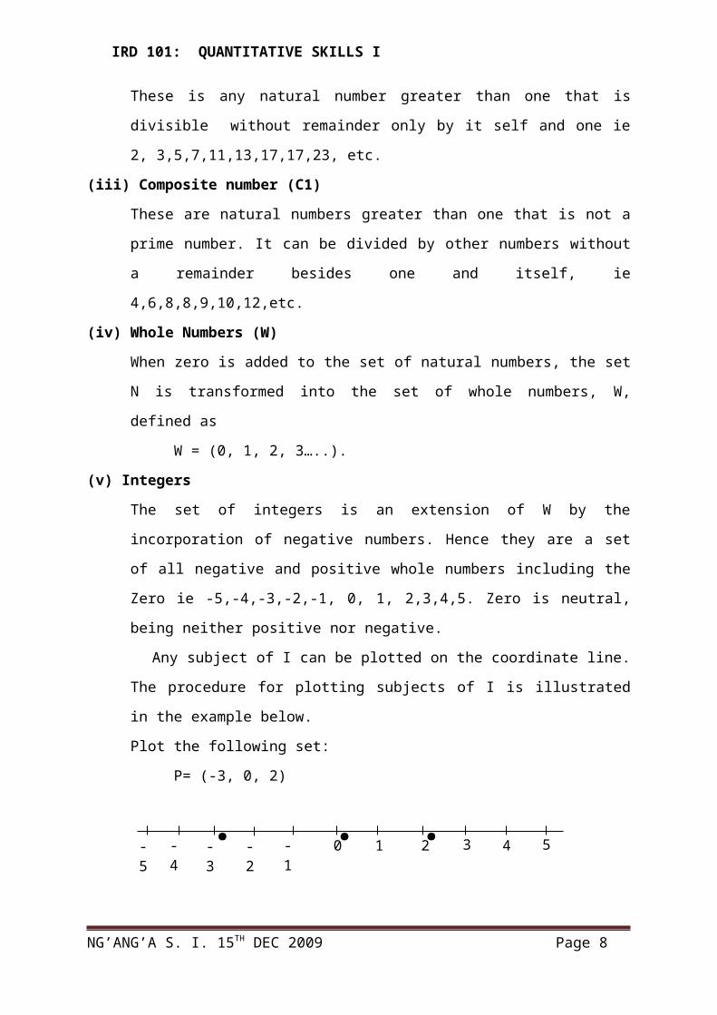
Any subject of I can be plotted on the coordinate line. The procedure for plotting
subjects of I is illustrated in the example below.
Plot the following set:
P= (-3, 0, 2)
Rational numbers Vs irrational numbers. (Q).
A rational number is a number of the form in which a and b are integers with no common
factor ( if there is a common factor, it should be cancelled) eg = ½ where b is not supposed
to be 0 ie b≠ 0 but b can be 1 and other numbers a can be larger than b eg
Irrational numbers
Irrational numbers are the opposite of rational numbers. the set of irrational numbers ,
is the set of all those numbers which cannot be expressed as a ratio of the integers. Π,
2 and 3, are examples of irrational numbers.
A simple way of disguising rational from irrational numbers with decimals is to study
their decimals. The decimals of rational numbers are periodic or repeating decimals,
whereas irrational numbers have non-periodic or non repeating decimals.
Is a rational number which has always been used as an approximation of the
irrational number π.
The decimal of π are non-periodic and are given below.
π = 3.14159265358….
However the decimals of 22/7 are periodic with a periodicity of 6.
= 3.14285714285714…
NG’ANG’A S. I. 15TH DEC 2009 Page 7
-5 -4 -3 -2 -1 0 1 2 3 4 5. ..
IRD 101: QUANTITATIVE SKILLS I
Real numbers (r)
Between any two rational numbers we have at least one irrational number, and,
conversely, between any two irrational numbers there is at least one rational number.
Hence the irrational numbers fill in the gaps between rational numbers and vice versa.
This process results in a continuum numbers constituting the set of real numbers.
Thus, A set of all rational numbers.
A real number can be represented as decimals eg – 1/6 = - 0.166….., ½ = 0.5, 1/3 =
0.33…, 2 = 1.4142, π = 3.141…
However, some real numbers may not necessarily be written in the decimal points eg natural
numbers and integers which also belong to the set, ie 3, 5, -1, -2, etc.
e.g. the subset -3 ≤ x < 2of R is shown below as a continuous line.
Another way of visualizing a set of real numbers is that every real number is used as a
co-ordinate for appoint on the number line. Therefore there is 1:1 correspondent
between the set of real numbers and the number line.
1.2 Properties1. Equality property
If x, y & z are real numbers and x=y then we can say that:
x + z= y + z
x – z = y – z
x z = y z
x/z = y/z if z ≠o
2. Reflexive property
If a is any real number, then a = a. any real number is equal to itself.
3. The symmetric property
If a, b, are real numbers and if a = b, b = a
4. The transitive property
NG’ANG’A S. I. 15TH DEC 2009 Page 8
-5 -4 -3 -2 -1 0 1 2 3 4 5.
R-Line

IRD 101: QUANTITATIVE SKILLS I
If a, b, and c are real numbers and if a = b and b = c then a = c.
If one number is equal to a second and if the second number is equal to the third then
the first number is equal to the number.
5. The substitution property
If a and b are real numbers and a = b then b can be substituted for a in any
mathematical expression to obtain an equivalent expression.
Examples:
1. x -3 = x -3 Reflexive
2. if 5x = 3y then 3y = 5x – Symmetric
3. if 6x = 10 and 3y = 10 then 6x = 3y (Transitive)
4. x + 4 = x y and x = 2 then 2 + 4 = 2y (substitution)
6. The closure property
If a and b are real numbers then a + b is a real number,
a – b is real no.
a X b is Real No
a/b is real no. provided b ± 0
Clause property guarantees that the sum, difference, product and quotient of any 2
real numbers are a real number, provided there if NO division by Zero (0).
7. Associative property
If a, b and c are real No.s, then (a + b) + c = a +(b +c), and (a b)c = a(bc). This
property permits us to group or associate the numbers in a sum or product in any way
that we wish.
Example:
(4 + 5) + 6 = 4 + (5 + 6 ) = 15
(2.3) .4 = 2. (3.4) = 24
8. Commutative property
If a and b are real numbers, then a + b = b + a and also a b + b a. These property
permits that addition and multiplication of any 2 real numbers to be done is either
order gives the same answer.
NG’ANG’A S. I. 15TH DEC 2009 Page 9

IRD 101: QUANTITATIVE SKILLS I
9. The distributive property of multiplication and addition
If a, b and c are real numbers then a (b +c) = a b +a c.
10. Identity elements and diverse elements
(i) Additive elements
0 is the addictive identity elements because by adding 0 to any real number, the
number remains the same e.g. a + 0 = 0 + a = a
(ii) 1 is the multiplicative identity elements since a 1 = 1 a = a where a in the case
of (i) and vice versa.
Since a + (-a) = (-a) + (+a) = 0
Is called the reciprocal of the multiplicative inverse of a. Also a is the reciprocal of
multiplicative inverse of provided a ± 0
i.e. = a= 1
NB: The reciprocal of 0 does not exist because there is No number that can be multiplied by 0
to get 1.
1.3 Arithmetic of real numbersIf 2 real numbers have like signs, their sum is found by adding their common sign i.e.
a + b = (a) + (b) = + (a + b)
a-b = (a) + (-b)
If two real numbers have unlike signs their sum is found by subtracting their absolute values.
The smaller from the larger and using the sign of the number with greater absolute value.
Example:
x – y = x + (-y)
5- 10 = -2
The product or the quotient of the real numbers with unlike signs is the –ve of the product or
quotient of their absolute values.
2 X 4 = 8
2 X -4 =-8
= - 4
Order of operations
If an expression does not contain grouping symbols then,;
(i) Evaluate any exponential expression like xy
NG’ANG’A S. I. 15TH DEC 2009 Page 10
IRD 101: QUANTITATIVE SKILLS I
(ii) Do all multiplication and division as they are encounter working from the left to
the right.
(iii) Do all additions and subtractions as they are encounter working from left to right.
If an expression contains grouping symbols use the above rules to perform the
calculation within each pair of grouping symbols from the inner most pair.
Example:
2x2 + (x +1)2 + 4 when x = 1
2 (1)2 + (1 + 1)2 + 4
2 + 4 +4 = 10
1.4 Fractions and their propertiesProperties:
1. Assume the following fractions and , & d 0 and if b 0 then, we conclude
that = if ad = b c and this property is property of equality.
Example:
=
9 49 = 7 63 because the product are equal then the fraction are equal.
2. If a is a real number then = a and if a ≠ 0 then = 1
Example:
= 1, = 6
3. Fraction are multiplied and divided according to the following definitions:
(i) = = provided b≠ 0& d≠ 0
(ii) ÷ = = provided d 0, b 0, c 0
Example:
÷ = =
÷ = = = ¼÷ = =
4. Scaling factor
If b≠ 0 and R≠0 then, = = ÷ =
Example:
NG’ANG’A S. I. 15TH DEC 2009 Page 11

IRD 101: QUANTITATIVE SKILLS I
= = ÷ =
This property can also be used to build fractions by inserting common factors in both
numerator and denominator.
Example:
Write with a denominator of 30.
Common factor = 6.
is ÷ = .
5. Signs
= = = - =
6. Fractions are added ands subtracted according to the following definitions:-
If b ≠ 0 then;
+ =
+ =
Show that;
+ = provided that b≠0, d ≠ 0
1.5 Algebraic FractionsThe rule governing the use of Algebraic fractions are identical to those used in ordinary
fraction.
1. Simplification of algebraic equations
Fractions may be simplified by removing a common factor from both numerator and
denominator.
Example:
Common factor = 9b x
=
2. Adding and subtracting of algebraic expressions
NG’ANG’A S. I. 15TH DEC 2009 Page 12
IRD 101: QUANTITATIVE SKILLS I
Fractions have to have a common denominator before they can be added or
subtracted.
Example:
Common denominator 6
3 (x + y) +2 (x – y) = 3x + 3y + 2x – 2y
6 6
= 5 x – y
6
3a -2b – 3b – a common denominator is ab2
A b b2
ab2 3a -2b – 3b – a
a b b2
3ab – 2b 2 – 3ab + a 2
Ab2
-2b 2 +a 2 = a 2 –2 b 2
Ab2 ab2
3. Multiplication and division of fractions:
Example:
x 2 – 1 3x – 6
x2 – 2x 4x + 4
Factoring and simplifying, we have
(x +1) (x – 1) X 3(x -2)
x(x – 2) 4 (x + 1)
= 3 (x – 1)
4x
Assign.
a b 1 = a b a –b
A2-b2 a –b (a -b) (a+b) 1
= a b
a + b
Simplifications of complex fractions
NG’ANG’A S. I. 15TH DEC 2009 Page 13
[ ]
÷

IRD 101: QUANTITATIVE SKILLS I
Example:
a 2 – b 2 ÷ a + b = a 2 – b 2 3
a 3 b a + b
= (a –b) X 3 = 3(a –b )
a b
QUIZ: Change a- b to an equal factor whose denominator is d-c
c –d
1.6Revision questions1. State whether each of the following sets is finite or infinite and justify your answer.
i. {x:x is a rational number} 2 mks
ii. {y:y is a country in the word} 2 mks
iii. {z:z is a student in a Kenyan university} 2 mks
2. List the members of the setQ={r:r€T=3r+1 for r=0,1,2,3}What is n (Q)? 3mks
3. a) State whether each of the following is finite or infinite and in each case justify your answer.
(i.) A=[x:x is a whole number] 2mks(ii.) B=[x:4<x<20; x is a rational number] 2mks
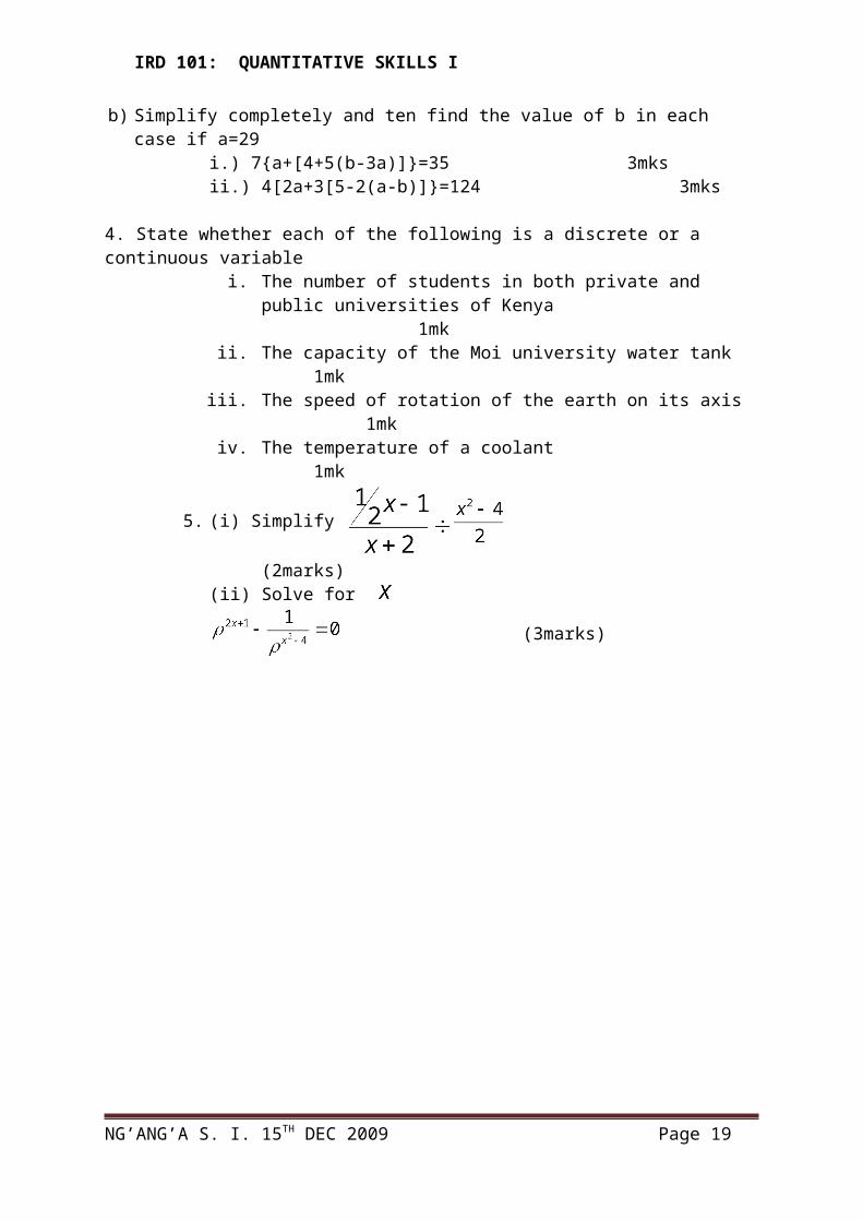
b) Simplify completely and ten find the value of b in each case if a=29i.) 7{a+[4+5(b-3a)]}=35 3mksii.) 4[2a+3[5-2(a-b)]}=124 3mks
4. State whether each of the following is a discrete or a continuous variable i. The number of students in both private and public universities of
Kenya 1mkii. The capacity of the Moi university water tank 1mk
iii. The speed of rotation of the earth on its axis 1mkiv. The temperature of a coolant 1mk
5. (i) Simplify (2marks)
(ii) Solve for
(3marks)
NG’ANG’A S. I. 15TH DEC 2009 Page 14

IRD 101: QUANTITATIVE SKILLS I
2.0 BASIC SET THEORY2.1 Introduction
A set is a fundamental concept in all branches of mathematics.
DEFINITION: A set is any well defined list, collection, or class of objects. An object in set
can be anything i.e. numbers, people, letters, rivers, mountains etc. these objects are called
the elements or numbers of the set.
Set notations
Sets are usually denoted by capital letters i.e. A,B,C, D etc. the elements or members in set
are usually represented by lower case letters i.e. a, b ,c, d etc.
2.2 Types of sets1. Numerative sets
2. Discriptive sets.
1. Numerative sets:
If we define a particular set by actually listing its ,member e.g. let A consist of the numbers
1,3,7 and 10, then we write a set as A = (1,3,7,8,10). Numerative i.e., the elements are
separated by, comas and closed in brackets ( ). This is a Tabular form of a set.
2. Discriptive sets
If we define a particular set by stating properties which its elements must satisfy eg let B be
the set of all even numbers, then we use a letter usually x to represent an arbitrary element
and we write.
B = (x/x is even), which reads as B is the set of numbers x such that x is even. We call
this the set builder form of set.
B = (x: x is even)
NB/: The vertical line or 2 dots(:) is read as that
2.3 Set Concept and Their Symbols1. Sets of sets
Sometimes it will happen that the object of a set are sets themselves e.g. the set of all subjects
of A. it is also known as family of sets or class of sets.
The symbol used are the script letters e.g. Β, etc
NG’ANG’A S. I. 15TH DEC 2009 Page 15

IRD 101: QUANTITATIVE SKILLS I
1. Universal set U or Σ
The family of all the subset of any set (S) is called the power set of S. we denote the power
set of S a2 2s
Let M = {a, b}
Then 2M = { (a, b), (a), (b), φ}
Let T = { 4,7,8}
2T = {(4,7,8), (4,7) (4,8)(7,8) (4) (7) (8), φ}
If a set is finite say S has n elements then the power set of S can be shown to have 2n
elements. This is one reason why the class of subjects of S is called the power set of S and is
denoted by 2s.
4. Disjoint set
If sets A and B have no elements in common i.e. if no element of A is in B and no element of
B is in A then, we say A and B are disjoint.
Example:
Let A ={1,3,7,8}
B = { 2,4,7,9} then A and B are not disjoint.
Since 7 is in both sets.
Q 2:
Let A be the +ve and B be –ve numbers. Then A and B are disjoint set since no number is
both –ve and +ve.
5. Comparability sets.
Two sets A and B are said to be comparable if ACB or BCA i.e. if one of the sets is a subject
of the other set. However, two sets A and B are said to be not comparable if A ± B or B ± A.
NB:
If A is not comparable to B then there is an element in A which is not in B and also there is
an element in B which is not in A.
Example:
Let: A = { a,b}
B { a,b,c}
A is comparable to B since A is a subject of B but we cannot say B is comparable to A
because B is not a subject of A.
NG’ANG’A S. I. 15TH DEC 2009 Page 16

IRD 101: QUANTITATIVE SKILLS I
R = {a,b)
C = { b,c,d}
R and C are not comparable since a is not in C i.e. R ± C, C± R.
6. Subsets
If every element in a set A is also a member of a set B then A is a subset of B if x is a
member of A. it implies that x is an element of A and B i.e. { xEA= xEB}
We denote this relationship by writing ACB which can also be read as A is contained in B.
Example 1.:
The set C is given by elements C = {1,3,5}
D = {5,4,3,2,1} since each element 1,3,5 belonging to C also belongs to D.
If E = {2,4,6} and F = {6,2,4}, since each element 2,4,6 belonging to E also to F
NB: let G = {x1 X is even } i.e.
G = {2,4,6,8…}
F = { x 1x is a positive power of 2}
I.e. F = { 2,4,8,16…..}
Then F is a subset or contained of G.
Definition:
Two sets A and B are equal i.e. A = B iff ACB and BCA. If ACB then we can also write B
A. if A is not a subset of B.
Conclusion:
1. The null set is considered to be subset of every set.
2. If A is not a subset of B, then there is at least one element in A that is not a member of
B.
Proper Subsets
Since every set A is a subset of itself then we call B a proper subset of A if
(i) B is a subset of A i.e. BCA
(ii) B is not equal to A i.e. B ≠ A
In some books B is a subset of A denoted by BCA = BCA and B is proper subset of A is
denoted by BCA.
Null set (ф)
Empty set/null set is a set that contain no elements. Such a set is void or empty and we denote
it by the symbol ф.
NG’ANG’A S. I. 15TH DEC 2009 Page 17

IRD 101: QUANTITATIVE SKILLS I
Example:
Let B = {x1x2 =4} and is defined as odd
Then, B = { }
Equality of sets
Set A = set B if they both have the same members i.e. if every element which belongs to A
also belongs to B and if every element which belongs to B also belongs to A we denote by A
= B.
Example:
Let A = {1,2,3,4}
B = {3,1,4,2}
A = B or { 1,2,3,4,2} = {3,1,4,2}, because all members belonging to A belongs to B.
NB: repetition is not recognized. A set does not change if its element are repeated.
Example 3:
E= {x1x2 – 3x = -2}
E = {2,1},
G = {1,2,2,1}
Therefore E = F = G
2.4 Finite and Infinite SetsSets can be finite or infinite. A set is finite if it consists of a specific number of different
elements i.e. if in counting the different members of the set the counting process come to an
end otherwise a set is infinite.
Example: Let M = {days of the week} finite
N = { 2,4,6,8…} N is infinite
P = { x1x is a river on the earth} therefore P is finite although it
may be difficult to count the number of rivers in the the earth, P
is still a finite set.
2.5 Complement of a SetIf A is any set which is a subject of a universal set then the complement of A normally
written as A1 or Ac is defined as all those elements that are not contained in A but are
contained in U or E.
NG’ANG’A S. I. 15TH DEC 2009 Page 18
IRD 101: QUANTITATIVE SKILLS I
Example:
E = {1,2,3,4,5,6,7,8,9}
A = {2,3,4,8}
Ac or A1 = {1,5,6,7,9}
2.6 Overlapping Sets
If sets A and B have same elements but these are not subsets of another set then, these are
called overlapping sets. E.g.
A ={1,2,3,4}, B = {3,4,5,6,7) = A¢ B
3 and 4 are common elements then they are overlapping set.
2.7 Product of SetIf A and B are any two sets, then the product of A and B denoted by A X B consist of all
ordered pairs (a,b) where a is an element of A and b an element of B.
Hence A X B = { (a,): aEA, bEB}
The product of a set with itself is A X A= A2
Example:
Let A = {1,2,3} and B = {a, b}
Then A X B = {1,a), (1,b), (2,a), (2,b), (3,a), (3,b)}
The concept of product set is extended to any finite number of sets in a natural way. The
product set of the sets A1, A2, A3…., Am is the set of all ordered in triples i.e. a1, a2, a3,
……… am where a:E A; for each is;
Example: Let M = {Tom, Mark, Eric}
W= {Andrew, Betty}, Find M X W
MXW = {(Tom, Audrey), (Tom, Betty), (Mark, Audrey), (Mark, Betty), (Eric, Audrey),
(Eric, Betty}
If we let A = {1,2,3}, B = {2,4} and C = {3,4,5}
Find A X B X C
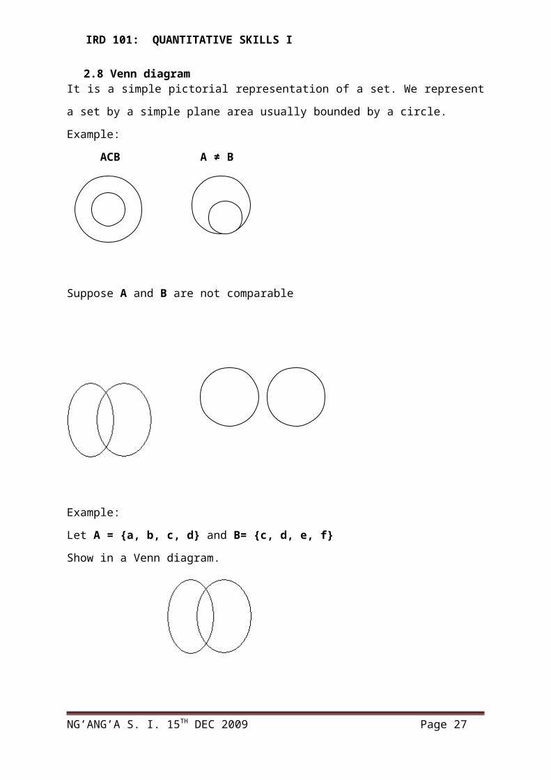
2.8 Venn diagramIt is a simple pictorial representation of a set. We represent a set by a simple plane area
usually bounded by a circle.
Example:
NG’ANG’A S. I. 15TH DEC 2009 Page 19

IRD 101: QUANTITATIVE SKILLS I
ACB A ≠ B
Suppose A and B are not comparable
Example:
Let A = {a, b, c, d} and B= {c, d, e, f}
Show in a Venn diagram.
NG’ANG’A S. I. 15TH DEC 2009 Page 20

IRD 101: QUANTITATIVE SKILLS I
2.9 Basic Set OperationIn the set theory, we define the operation UNION INTERSECTION & DIFFERENCE i.e. we
assign new sets to pair of sets A & B
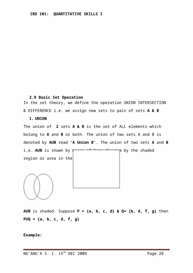
1. UNION
The union of 2 sets A & B is the set of ALL elements which belong to A and B or both. The
union of two sets A and B is denoted by AUB read ‘A Union B’. The union of two sets A and
B i.e. AUB is shown by means of Venn diagram by the shaded region or area in the following
diagrams.
AUB is shaded. Suppose P = {a, b, c, d} & Q= {b, d, f, g} then PUQ = {a, b, c, d, f, g}
Example:
Let ℓ be the set of positive real numbers and M be set –ve real numbers. what is ℓ UM
= the set of all real numbers except 0.
Thus the union of AUB = {x1xEB}. We can conclude directly from the definition of A and B
that AUB and BUA are the same set ie AUB =BUA.
Similarly we conclude that both sets A and B are always subsets of AUB ie
AC (AUB)
BC(AUB)
NB: in some books + is used instead of U and is called the theoretic sum which reads A+ B ie
“A plus B’.
NG’ANG’A S. I. 15TH DEC 2009 Page 21
IRD 101: QUANTITATIVE SKILLS I
2. INTERSECTION
Intersection of two sets A and B is the sets of elements which are common to A and B ie
those elements which belongs to A and also belong to B. the intersection of A and B is
denoted by AnB which is read ‘A intersection B’. the intersection of two sets A and B ie An
B is shown by means of Venn diagram by the shaded region that is common to both A and B.
Example: If we let P = {2,4,6,…..} i.e. multiple of 2
And Q = {3,6,9……} multiple of 3.
Then PnQ = {6, 12,18,24,30 ……..}
Example: if we let L = {a, b, c, d} & M ={f, b, d, g,}
Then ℓn M = {b, d}, hence intersection of two sets A and B can also be defined as AnB =
{x1xEA and xEB}. This we can conclude directly from the delimitation of the intersection of
two sets that is AnB = BNA. Similarly we also conclude that each of the sets A and B as a
subset i.e.
(AnB) CA
(AnB) CB
In the same way it sets A and B have no elements in common ie A and B are disjoint then the
intersection of A and B is null set i.e. AnB = ф
DIFFERENCE
The difference of two sets A and B is the set of elements which belong to A but which do not
belong to B. the difference of two sets A and B is denoted by A –B and is read as A
difference B or A minus B. the difference of two sets A and B is also sometimes denoted by
A/B or A2B read as A given B.
The difference of two sets A and B ie A – B is shown by Venn diagram by the shaded area/
region in A which is not part of B.
NG’ANG’A S. I. 15TH DEC 2009 Page 22

IRD 101: QUANTITATIVE SKILLS I
Example:
Let P = {a,b,c,d} and Q = {b,d,f,g}
Then P –Q or P ~ Q or P/Q = {a,c} or Q-P ={f,g}
Example:
Let L be set of real numbers and M be the set of rational numbers. Then L – M consist of the
irrational numbers thus the difference of two sets A and B can also be defined as:
A – B = {x1xEA and x ≠ B}.
Thus we conclude that set A contains A – B as a subset i.e. (A – B) CA and the sets A –B,
AnB and B –A are mutually disjoint i.e. the intersection of any two of the sets is the NULL
SET.
COMPLEMENT
Given any two sets, A and B, then we can get Ac and Bc
Example: let A {a, b, c, d} and B= {c, d, e, f}
Then,
Bc = {a,b} and Ac = {e, f}
In a Venn diagram:
NG’ANG’A S. I. 15TH DEC 2009 Page 23

IRD 101: QUANTITATIVE SKILLS I
Ac is shaded
Facts about sets which follow directly from the definition of the complement of the set.
1. (a) The Union of any set and its complement A1 is the universal set i.e. AUA1 = E
(U).
(b) Set A and its complement i.e. An A1 is disjoint i.e. AnA1 = ф
2. The complement of the universal set is the null set and vice versa i.e. U1 = ф and ф =
U.
3. The complement of the complement of the set A is the set itself i.e. (A1)1 = A.
4. The difference of A and B equal to the intersection of A and complement of B ie A – B =
An B1.
We also follow directly from the definition that A – B = {x1xEA, xEA} =
{x/xEA,xEA,XEB1} = AnB1
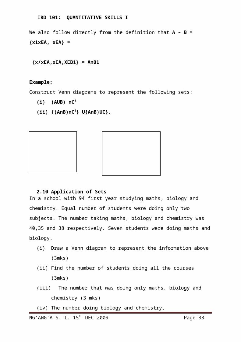
Example:
Construct Venn diagrams to represent the following sets:
(i) (AUB) nC1
(ii) {(AnB)nC1} U{AnB)UC}.
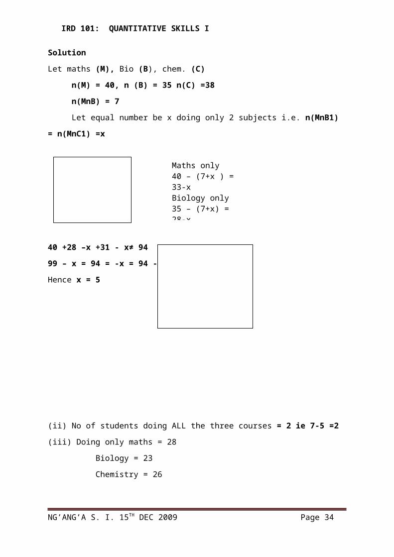
2.10 Application of SetsIn a school with 94 first year studying maths, biology and chemistry. Equal number of
students were doing only two subjects. The number taking maths, biology and chemistry was
40,35 and 38 respectively. Seven students were doing maths and biology.
(i) Draw a Venn diagram to represent the information above (3mks)
(ii) Find the number of students doing all the courses (3mks)
(iii) The number that was doing only maths, biology and chemistry (3 mks)
(iv) The number doing biology and chemistry.
NG’ANG’A S. I. 15TH DEC 2009 Page 24
IRD 101: QUANTITATIVE SKILLS I
Solution
Let maths (M), Bio (B), chem. (C)
n(M) = 40, n (B) = 35 n(C) =38
n(MnB) = 7
Let equal number be x doing only 2 subjects i.e. n(MnB1) = n(MnC1) =x
40 +28 –x +31 - x≠ 94
99 – x = 94 = -x = 94 -99 =-5
Hence x = 5
(ii) No of students doing ALL the three courses = 2 ie 7-5 =2
(iii) Doing only maths = 28
Biology = 23
Chemistry = 26
(iv) No. of students doing Biology and Chemistry = 7. ie 5 +2 = 7
Example 2.
Given n(E) = 84
n(AnB) = 4
n(AuBuC)1 = 3
n(AnC)= n(BnC) = 7
n(A) = 30, n(B) = 40, n(C) =28.
(i) Draw a Venn diagram to show this information (3mks)
NG’ANG’A S. I. 15TH DEC 2009 Page 25
Maths only40 – (7+x ) = 33-xBiology only35 – (7+x) = 28-xChemistry only38-(7+x) = 31-x
IRD 101: QUANTITATIVE SKILLS I
(ii) Find the number of elements
n(AnBnC) (2mks)
n(AnB)nC1 (2mks)
n(A1nC1) (2mks)
n(AuB)1nC (2mks)
let n(AnBnC) =x
Hence 30 +14+x 7- x+ 29 + x3 = 84
83 +x = 84 = x = 84 -83 = 1
n(AnBnC) =1
n(AnB)nC1 = 3
n(A1nC1) = 30 + 3 = 33
n(AuB)1nC = 15
Example 3
in a café with Average of 440 customers a week, it was found that like chicken, 150 beef and
200 Githeri. It was also found that same number of customers liked both chicken Githeri, one
NG’ANG’A S. I. 15TH DEC 2009 Page 26
IRD 101: QUANTITATIVE SKILLS I
third of the same number liked chicken and beef and only a sixth of those liking Githeri and
beef liked all the three foods. Find the number of customers liking
(i) Chicken only(3 mks)
(ii) Beef only (3mks)
(iii) The No. of customers who liked all the three foods (3mks)
NG’ANG’A S. I. 15TH DEC 2009 Page 27
IRD 101: QUANTITATIVE SKILLS I
2.11Revision questions1. In the school of business and economics, lecturers Kamau, Kiprono, Wekesa and Munyao have masters’ degrees, with Kamau and Munyao also having Doctorate degrees. Kamau, Otieno, Wekesa, Nyevu, Ekeru and Okware are members of institute of certified public accountants of Kenya (ICPAK) with Nyevu and Ekeru having masters’ degree. Identify set A as those lecturers with masters’ degree; set B as those who are ICPAK members and set C as doctorate holders.
a.) Specify the elements of AB and C 6mksb.) Draw a diagram representing sets A,B and C together with their known elements
5mksc.) What special relationship exists between set A and C? 2mksd.) Specify the elements of the following sets and for each set, state in words what is
being conveyed?i.) A n B ii.) C u B and iii.) C n B 3mks each
e.) What would be suitable universal set for the scenario? 3mks2. a) In a class of 17 students it was found that some were Blood A,B and O. the number of students with Blood group A were 9. The following additional information was also available;
n(AnBnO)=n(A n B O’)n(B’UA’) 11n(A’ n B’)=n(A’n O’)=n(B’ n O’)n(AnOnB’)=2
Given also that:AB+ I in the region (A n B n O)O+ is in the region BnOnA’A+ is in the region AnOnB’Required Draw a Venn diagram illustrating the information and find the numbers of students who were blood group: 5mksi.) AB+ 3mks ii) A+ 3mks iii) O+ 3mks b) The total number of students Registered in a department of Kileti University for three courses A, B, C was 16,500. the lowest enrolled course had 6000 less than the highest and 3,500 less than the second highest. How many students registered for each of the three courses? 6mks
3. Given the following sets that n(ڭ)=7, n(A’) =4, n(AnB)=1, n(B)=3 Find:i.) n(A) 2mksii.) n(B’uA) 2mks
state whether it is correct or not to rite and why?iii.) Aeڭiv.) A’cڭv.) (AnB)eA 6mks
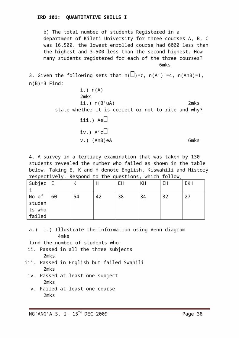
4. A survey in a tertiary examination that was taken by 130 students revealed the number who failed as shown in the table below. Taking E, K and H denote English, Kiswahili and History respectively. Respond to the questions, which follow;Subject E K H EH KH EH EKH
NG’ANG’A S. I. 15TH DEC 2009 Page 28
IRD 101: QUANTITATIVE SKILLS I
No of students who failed
60 54 42 38 34 32 27
a.) i.) Illustrate the information using Venn diagram 4mks find the number of students who:
ii. Passed in all the three subjects 2mksiii. Passed in English but failed Swahili 2mksiv. Passed at least one subject 2mks v. Failed at least one course 2mks
vi. Failed in two subjects 2mksvii. Passed in History 2mks
viii. Passed English or Swahili 2mksb.) using set notation symbolically represent the information in a.) above from question ii.) to vii.)
5. a) Distinguish between the following terms as used in set theory:i.) Equivalent sets and equal sets 2mks
ii.) Disjointed sets and sub sets 2mks b.) The main daily newspapers in a country are: the National, The New Era and the
Citizen. The management of one of the dailies was concerned about the sales volume of their papers. In a survey of 100 families conducted in the country, the numbers that read the various newspapers were found to be as follows:
Name of the newspaper Number of readers The citizen 28The citizen and New era 8The new era 30Citizen and National 10The national 42New era and National 5All the three papers 3
Requiredi.) Present this information in a Venn diagram 4mks ii.) determine the number of families who did not read any of the three
newspapers 1mkiii.) calculate the number of families that read only one of the newspapers
3mks
6. a) In a market survey by a beverage manufacturer, it was found that all the people interviewed drank Milo or coffee. Half of the people drink Milo only, two drink both Milo and coffee and seven drink coffee only.
i.) Illustrate this information in a Venn diagram 3mks ii.) Determine how many people were interviewed 3mks
NG’ANG’A S. I. 15TH DEC 2009 Page 29

IRD 101: QUANTITATIVE SKILLS I
b) A random sample of 400 university students found the following habits: 130 wore sunglasses, 135 wore short trousers and 125 wore caps. If 35 wore sunglasses and short trousers, 40 wore short trousers and caps, 45 wore caps and sunglasses and 126 did not wear any of the three items.i.) using a Venn diagram, determine how many students wore all three items 10mks ii.) Find out how many students wore any combination of the two items 4mksiii.) Calculate how many students wore only one of the items 4mks
7. a) There are 54 students in Mgecon College. 30 of them take mathematics; 26 take economics and 21 take geography. The following additional information is also provided to you.
13 students take maths and economics 12 students takes maths and geography 11 students take geography and economics 4 students take maths and geography only
Required i. Write the above information in a set notation 4mks
ii. Present the above information in the form of a Venn diagram 4mksiii. How many students take all the three subjects? 2mksiv. How many students take none of the three subjects? 2mksv. How many of the students take two subjects only? 2mks
vi. How many students take one subject only? 2mks b.) Given that A={t,u,v}list all the subsets of A 2mks
8. a) Using a Venn diagram, illustrate the following sets(i) (A B) (2marks)(ii) (3marks)b) In a village in Nyawara District, three mobile telephony Networks exist. It has been
established that the adult residents of the village numbering 500 all access the mobile telephone services by use of Safaricom, Zain or Orange. The majority (300) use Safaricom, 150 uses both Safaricom and Zain only while 200 use Orange. The same number of customers uses Zain only as do Orange only. A half of that number use both Safaricom and Orange, while a third of that number uses Zain and Orange.
Determine the number of residents who use;(i) Safaricom only (2marks)(ii) Orange only (2marks)(iii) Zain only (2marks)(iv) All the three networks (2mark)(v) Safaricom and Zain only (1marks)(vi) Safaricom and Orange only (2marks)(vii) Zain and Orange only (2marks)
NG’ANG’A S. I. 15TH DEC 2009 Page 30

IRD 101: QUANTITATIVE SKILLS I
3.0 COMPUTATION SKILLS3.1 Exponents and Logarithms3.2Definition:
Exponents, base, matrix, characteristics, logarithms standard forms. A number written with
one digit to left of the decimal point and multiplied by 10 raised to some power is said to be
written in standard form.
5837 = 5.837 X 10³
0.0415 = 4.15 X 10 -2
When a number is written in standard form the first factor is the mantissa and the second
factor is called the exponent.
Thus 5.8 X 10³ has a mantissa of 5.8 and exponent of 103
2000 = 2X2X2X2X5X5X5 = 24 X53
2 and 5 are bases whereas 4 and 3 are indices.
When an index is an integer it is called a power, hence 24 is called 2 power 4
Special names may be used when the indices are 2 and 3. they are called squared and cubed
respectively.
NB: when no index is shown then the power is 1.
3.2 Law of Exponents or Indices
1. When multiplying two or more numbers have the same base the indices are add thus
am X an = a m+n
Let a = 3 32 X 34 = 3 2+4 = 36
2. When a number is divided by a number having the same base the indices are subtracted.
am ÷ an = am/an = a m-n
35 ÷ 32 = 35/ 32 = 35-2 = 33
3. When a number which is raised to a power is raised further to another power the indices
are multiplied e.g.
(am)n = amn
(35)2 = 35X2 = 310
4. A number has an index of zero (0) its value is 1
a0=1
30 =1
5. A number raised to –ve power is the reciprocal of that number raised to +ve power.
NG’ANG’A S. I. 15TH DEC 2009 Page 31

IRD 101: QUANTITATIVE SKILLS I
a-n = 1/an
3-4 = 1/34
Similarly ½-3 = 23.
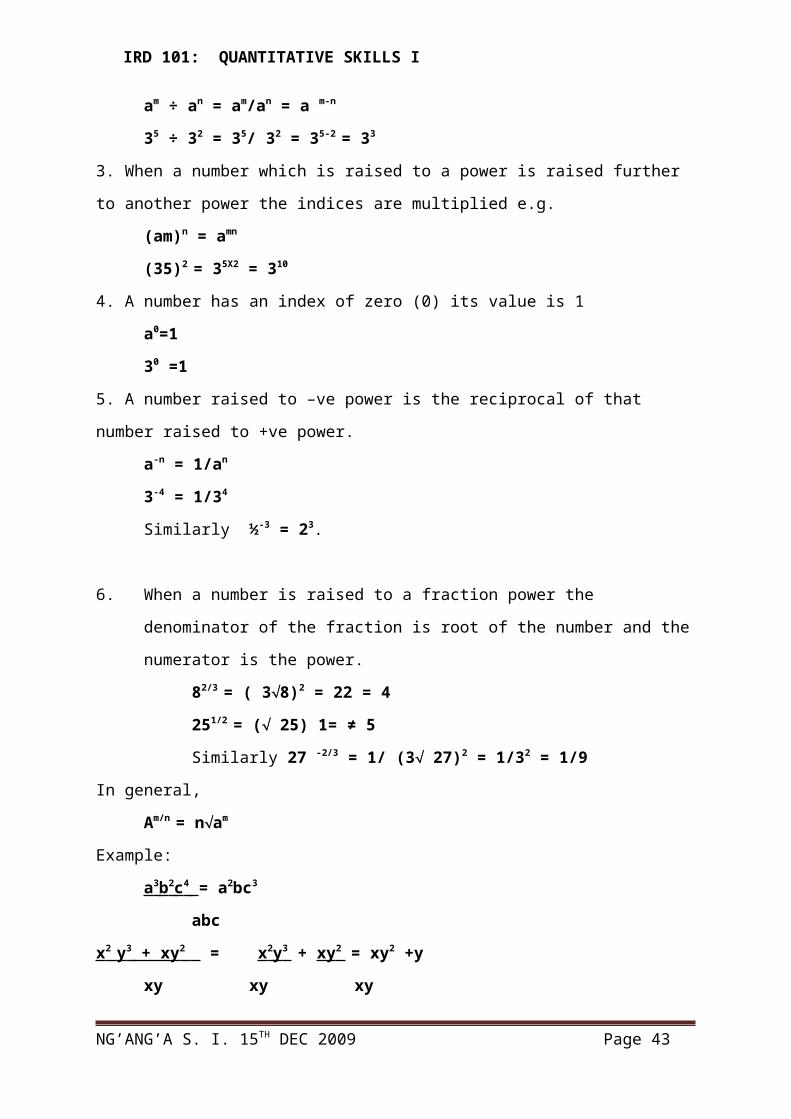
6. When a number is raised to a fraction power the denominator of the fraction is root of
the number and the numerator is the power.
82/3 = ( 38)2 = 22 = 4
251/2 = ( 25) 1= ≠ 5
Similarly 27 -2/3 = 1/ (3 27)2 = 1/32 = 1/9
In general,
Am/n = nam
Example:
a 3 b 2 c 4 = a2bc3
abc
x 2 y 3 + xy 2 = x 2 y 3 + xy 2 = xy2 +y
xy xy xy
x2y = x 2 y = x
xy2 – x y = x y(y-1) y -1
Quiz: simplify (Mn 2 ) 3 = M 3 n 6 = M 3 n 6 = Mn5
(M1/2n1/4)4 (M1/2)4(M1/4)4 M2n1
(x 2 y 1/2 ) ( x 3 y 2 )
(x5y3) 3/2
3.3 LogarithmsA logarithm of a number is the power to which a base has to be raised to be equal to the
number.
Y= ax
= x = logay
Log3a = x = log3a
3x = 9
NG’ANG’A S. I. 15TH DEC 2009 Page 32
IRD 101: QUANTITATIVE SKILLS I
3x = 32 = x =2
Hence log39 = 2
Log168 = x= log168 = 16x = 8
(24)x =23
4x = 3= x =3/4
Hence log168 = ¾
Example 2:
Log2y = 3
23 = y = 8
(ii) Logarithms having a base of L are called hyperbolic or napierian or natural logarithms.
Napierian logarithms of x = logex or more commonly lnx (natural log of x)
Ln 8.61 = 2.1529…
Ln 62179 =
Ln 0.149 = -9
The change of the base rule:
The change of base rule for logarithms states that:
Logay = logby
Logba
Let t = logay = at = y
Taking the logs to base b, we get
Logbat = logby
T logba = logby
= t = logby
Logba
3.3.1 Laws Of Logarithms1. Multiplication
Log (A X B) = log A + log B
2. Division
Log (A/B) = log A – log B
3. Power
Log An = nlogA
NG’ANG’A S. I. 15TH DEC 2009 Page 33
IRD 101: QUANTITATIVE SKILLS I
Example:
Log 64 = log 128 + log 32
= 6 log 2 – 7 log 2+ 5 log 2 = 4 log 2
2x = 3 (taking log2 to base 10)
Log 2x = log3 = x log2 = log3 = x= log 3 = 0.474 = 158
Log 2 0.3010
X3.2 = 41.15 = 3.2 log x = log 41.15
= log x = log 41.15
3.2
Using logarithms, evaluate
1295 X 1.2
4.8 32
No. Log
1295= 1.29 X 10² 3.1123
1.2 = 1.2 X 100 0.0792
3.1915
48. 32 = 4.832 X 101 1.6841
1.5074 = 3.216 X 101
Example:
1. 2.873
50.49 X 0.217
2. 3 0.7214 X 20.57
69.8
3. 2.935 X 0.07652
32.74
4. Show that log t x = 1/logxt
5. Calculate 372 1/3 X 0.56
457
6. Solve for x 23x = 5x+2
7. Show that logeb logbe = 1
NG’ANG’A S. I. 15TH DEC 2009 Page 34

IRD 101: QUANTITATIVE SKILLS I
Represent symmetric difference
A B, we are looking for elements that are only in A and only in B. eg A =
{ a,b,c}, B= {c,d,e}, then A B = {a,b,d,e}.
A B is shaded
(i) Show that log1618 = log23 (3mks)
(ii) 2loge (a-b) -2logea = log e(1 – 2b/a + b2/a2)
Solve for x in the following equations
(i) (1/2 log316 -1/3 log527)(log34 – ½ log59) = x
(ii) Log2x = log2e + log25
(iii) Given that log102 = 0.3010 & log 103 = 0.4771
Find log321
A log of a number is the power/ exponent to which the base is raised to get the same number.
(i) Express these notions in 2 equivalnet expression.
(ii) Solve for x = Log10 (x2 +2x) = 0.9037
(iii) Given that X is logb T, y = logbR, and z = log1 9
Show that = logaRT = x+y
Log Rx = xy
Log + = 1/z
Show that log38 = log83
Solve t if 1nt +1n9 +3n3
Solve 3 (x+1) = 120
Evaluate logaa-1/-1
Log2 (x+4) = log2x
Solve for x if loga (x2 + 2x) = 0.9031
Solve for t if Nt +N9 = 3 N 3
NG’ANG’A S. I. 15TH DEC 2009 Page 35

IRD 101: QUANTITATIVE SKILLS I
4.0 EQUATIONS4.1 Introduction
An equation is an expression with an equal sign. In equations, unlike in function, none of the
variables in the expression is designated as the dependent variable or the independent
variable although the variables are explicitly related.
Example:
3x + 4y = 13
- Equations can be classified into two main groups:
1. Linear equation
2. non – linear equation
- The two expressions below constitute examples of linear equations in the variable x.
x +13 = 15
7x + 6 = 0
- Non –linear equations in the variable x are equations in which x appears in the second
or higher degree.
5x2 + 3x + 7
2x3 + 4x2 + 3x + 8 = 0
4.2 Solutions of EquationsTo solve an equation involving a variable is to find the value or values of the variable for
which the equation holds. These values are called the roots of the equation and the set of
these values is referred to as the solution set.
Equations
An equation is a mathematical sentence/expression or an open statement containing one or
more variables. It has two sides (LHS & RHS), like a balance that they are equated by an
equal sign ‘=’ e.g. 4x + 8y = 25
Given the equation 4x + 8y = 25
i. i x and y constitute the variables of the equations which are found by solving the
equation. They are also known as unknowns and the values to these
unknowns/variables are called solutions or roots of the equation.
NG’ANG’A S. I. 15TH DEC 2009 Page 36

IRD 101: QUANTITATIVE SKILLS I
ii. 4, 8 and 25 are known as constants/parameters. They are fixed figures shown on the
left hand side of the unknown as separately.
iii. 4 and 8 are coefficients known on the lists of the unknown. They denote how many
times any specific unknown has been added.
iv. Given this type of equation 2x2 + 8x – 20 = 0, then the 2x2 has an index power 2. it
shows how many times x have been simplified by itself.
4.2.1 Categories of equation/types of equationsi) Linear or simple equations
ii) Quadratic equations
iii) Simultaneous equations
Linear equations
That which has unknown and the index of the unknown is one e.g. 4x – 10 = 0 : x is raised to
one i.e. x1 e.g.
Solve the equation:
2(4x – 2) = 3 (x +2)
8x – 4 = 3x + 6
8x – 3x = 6 +4
5x = 10
x = 2
Solve the following
i) 2x = 10 ii) x + 5 = 12 iii) x = 3x – 2 iv) 8 = 15
5 3 2 5 7 x
v) 3x = x + 9 vi) 3 + 3 = 4 vii) x +3 – x – 1 = 1
4 4 4 x 9 16 4 8
Quadratic equations
These are equations formed where the highest index/exponent of an unknown is 2 e.g.
X2 + 3x + 4 = 0
The standard for of a quadratic equation is ax2 + bx + c = 0
There are two methods primarily used to solve quadratic equations, namely:-
NG’ANG’A S. I. 15TH DEC 2009 Page 37
IRD 101: QUANTITATIVE SKILLS I
i) By factorization
ii) By formula
i) By Factorization
The part ‘bx’ is divided into two parts in such a way that b x b = a x c e.g.
Solve the equation 4x2 – x -3 = 0
Solution
4x2 – x – 3 = 0 look for two Nos. whose product would be -12 and same would be -1
4x2 – 4x + 3x – 3 = 0
4x(x – 1) + 3(x – 1) = 0
(4x +3) (x -1) = 0
Either 4x + 3 = 0 or x – 1 = 0
4x = -3 or x – 1
X= -3 and x=1
4
Check: b x b = a x c
-4 x +3 = 4x – 3
12 = 12
ii) By formula
Quadratic equations are solved using the following formula be
X = -b +
2a
Example:
Find the roots of the following equations.
(a) x2 + 5x – 4 = 0
(b) 5x2 – 3x = 4
Solution
X2 + 5x – 4 = 0 a = 1, b = 5, c = 4
Hence; substituting in the formulae:
X = -5 +
2 x1
ii) 5x2 – 3x = 4 a = 5, b= -3, c = -4
NG’ANG’A S. I. 15TH DEC 2009 Page 38
= 0.70 or 5.70

IRD 101: QUANTITATIVE SKILLS I
= 3 +
2 x 5
X= 3 +
10
X = 1.24 or x = - 0.64
4.2.2 Problems leading to quadratic equations:i) The length of a room is 4m longer than the width and the floor area is 92m2; find the length
and the breadth.
Solution
Length = (x + 4) m
Breadth = x
Floor area = Lx W = 96 i.e. x(x +4) = 96
X2 + 4x = 96 = x2 + 4x – 96 = 0
(x +12) (x – 8) = 0
Either x = -12 or x = +8
So take x = +8, since the breadth of the room cannot be negative.
ii) The sum of two digits is 10 and the sum of their squares is 58. find the digits
iii) If the average speed of a bus is reduced by 20Km/h, the time for the journey of 240Km is
by 1 hour. Find the average speed of the bus.
Simultaneous equations
These are equations whose numbers of unknown are two or more. If the numbers of the
unknown are two then the number of simultaneous equations must be 2. if the number of the
unknown are three then the number of simultaneous equations must be 3 e.g.
4x + 3y = 7
3x – 2y = 9
There are three methods of solving simultaneous equations, namely:-
i. Elimination
ii. Substitution
iii. Graphical
NG’ANG’A S. I. 15TH DEC 2009 Page 39
IRD 101: QUANTITATIVE SKILLS I
Elimination method
Solve the following equations
4x + 3y = 7
3x – 2y = 9
Here one of the unknowns has to be eliminated. We eliminate ‘Y, it would be
2x (4x + 3y = 7)
3x (3x – 2y = 9)
8x + 6y = 14
9x – 6y = 27
17x + 0 = 41
17x = 41
X = 41 2 7 and Y = 3 x 41 – 2y = 9
17 17 17
123 – 2y = 9
17
- 2y = 9 - 123
1 17
2y = 123 – 153
17
2y = -30
17
y = -30 2
17 1
y = -30 x 1
17 2
y = -30
34
y = -15
17
NG’ANG’A S. I. 15TH DEC 2009 Page 40
+

IRD 101: QUANTITATIVE SKILLS I
Substitution method
Given 4x + 3y = 7 …………………………….i
3x – 2y = 9 ……………………………ii
We can take the equation ‘i’ where we express x in terms of y, hence,
4x = 7 – 3y
x = 7 – 3y
4
Then, substitute this value of x into equation ii
3(7 – 3y) – 2y = 9
4
21 – y – 2y = 9
4
- 17y = 36 – 21
y = -15
17
By the value of y into 1
4x + 3 -15 = 7
17
4x – 45 = 7
17
4x = 7 + 45
17
4x = 119 + 45 4x = 164
17 17
X = 164 4 = 164 x 1 = 41 = 1/17
17 1 17 4 12
Graphical Method
i) Solutions of Linear Simultaneous Equations
Suppose you have prior mentioned equations and you are required to find their roots over
ranges
x+ y = 5
x- y =2
If x=0 to x if the following procedure is applied.
NG’ANG’A S. I. 15TH DEC 2009 Page 41

x +y = 5
x – y = 2
IRD 101: QUANTITATIVE SKILLS I
i. Let x + y = 5 be labeled I and given the values of x, get the values of y.
ii. Let x – y =2 be labeled ‘ii’ and given the values of x, get the respective values of y.
iii. draw a Cartesian system with x values moving
iv. Plot each of the equation in the system. Point of interaction forms the solution for
the equation.
v. In our case above, x = 3.5: y = 1.5: These values satisfy both equations
simultaneously.
Question 1
Graphically solve the equations
3.14x – 2.78y = 5.71
2.88x + 7.34y = 8.93
Over a range x = 0 to x = 5
Solution
x = 2.1 i.e. (2.1, 0.4)
y = 0.45
NG’ANG’A S. I. 15TH DEC 2009 Page 42
0
1
2
3
4
5
Y
1 2 3 4X
-1
-2
P(3.5, 1.5)
IRD 101: QUANTITATIVE SKILLS I
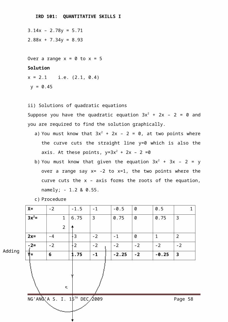
ii) Solutions of quadratic equations
Suppose you have the quadratic equation 3x2 + 2x – 2 = 0 and you are required to find the
solution graphically.
a) You must know that 3x2 + 2x – 2 = 0, at two points where the curve cuts the straight
line y=0 which is also the axis. At these points, y=3x2 + 2x – 2 =0
b) You must know that given the equation 3x2 + 3x – 2 = y over a range say x= -2 to
x=1, the two points where the curve cuts the x – axis forms the roots of the equation,
namely; - 1.2 & 0.55.
c) Procedure
X= -2 -1.5 -1 -0.5 0 0.5 1
3x2= 12 6.75 3 0.75 0 0.75 3
2x= -4 -3 -2 -1 0 1 2
-2= -2 -2 -2 -2 -2 -2 -2
Y= 6 1.75 -1 -2.25 -2 -0.25 3
Question
Solve the equation 2(x2 + 1) = 5x by graphical method over the range x=0 to x=3 i.e.
solutions line between x=0 to x=3
Answer: 0.5 and 2.0 (being the roots of the equation y=2x2 – 5x + 2 = 0
iii) Solutions of Linear and quadratic equations simultaneously.
NG’ANG’A S. I. 15TH DEC 2009 Page 43
Adding
0.5 1X
1
2
3
4
5
Y
-1
-2
0-0.5-1
-3
y= 3x2 + 2x – 2 (-1.2, 0.55)
(0.55)

IRD 101: QUANTITATIVE SKILLS I
Suppose you are given a linear and quadratic equation and you are needed to solve them
simultaneously e.g. y=2x2 – 5x + 2 and y=2x – 3 (straight line) over a range of x= 0 to x= 3
Solution procedure
i) Graph each of the equation on the same set of axes.
ii) Note their point of intersection
iii) Where the two graphs intersect give the solutions to the simultaneous equation
y=2x2 – 5x + 2 and y= 2x – 3. These points are (2.5, 2) and (1, -1)
NB: 0.5 and 2.0 are the roots of the equation 2x2 – 5x + 2 = 0
Suppose you have this equation
X1 + 2x2 + 3x3 = 3
2x1 +- 4x2 + 5x3 = 4
3x1 + 5x2 + 6x3 = 8
How would you find the values of X1, X2 and X3 (Hint use the substitution method)
Answer: X1 = 7, X2 = 5 and X3 = 2
NG’ANG’A S. I. 15TH DEC 2009 Page 44
y
x0
1
2
3
0.5 1 1.5 2 2.5
1
2
3
(1, -1)
(2.5, 2)
y =
2x2 –
5x +
2
y= 2x - 3

IRD 101: QUANTITATIVE SKILLS I
4.3 MATRICES4.3.1 IntroductionDEFINITION: It is a rectangular array/order of numbers called elements and it is represented
by writing down the elements and enclosing them in brackets.
Thus, Matrix algebra sometimes known as Linear algebra provides us.
1. With a concise method of writing system of linear equations.
2. With techniques for determining the existence of solutions to the system.
3. With a method of determining the solutions to the system.
Example: Consider the inventory of three farmers represented by the following matrix
F1 F2 F3
2 0 1
120 30 75
30 11 25
The matrix shows that the Farmer 1 has an inventory of: 2bags of Fertilizers: 120 bags of
wheat: and 30 bags of corn. The figures have been determined by reading down column 1,
which belongs to farmer 1.
Reading across row 2, the wheat row, we find farmer (F1) has 120 bags of wheat; farmer 2
(F2) has 30 bags of wheat and farmer 3 (F3) has 75 bags of wheat.
Thus, in matrix position and magnitude of each of the numbers in the matrix is of
considerable importance. E.g.
The column of farmer 2 and the third row, the entry is 11 bags of corn. The position of
number 11 is important because that specific location is reserved for the bags of corns
belonging to farmer two. The magnitude of the number is important since it specifies to us
the number of bags of corn belonging to farmers two.
Capital letters are used to designate a matrix and the number in the matrix referred to as
elements of the matrix are designated with small letter wit subscripts e.g.
a11 a12 a13 a14
A= a21 a22 a23 a24
NG’ANG’A S. I. 15TH DEC 2009 Page 45
Bags of fertilizer
Bags of wheat
Bags of corn

IRD 101: QUANTITATIVE SKILLS I
a31 a32 a33 a34
or
A = a15
Whereby i = The row in which element ‘a’ is found 1, 2, 3
ii = The column in which element ‘a’ is found 1, 2, 3, 4
The size of the Matrix is determined by the number of rows and columns the matrix has. In
our above example, the matrix has 3 rows and 4 columns and is said to be a matrix of order 3
by 4 written 3 x 4 matrix. The number of rows and columns of a matrix also constitute the
dimensions of the matrix.
The row dimension of our above example is 3 and the column dimension is 4
4.3.2 Types of Matrices 1. Equal matrices
Are those matrices that are identical. That is given two matrices A and B, they will be said to
be equal i.e. A=B if and only if they have the same number of rows, columns and elements in
the corresponding location e.g.
1 4 7 1 4 7
A= 2 5 8 B= 2 5 8
3 6 9 3 6 9
A=B
2. Column matrix or Column Vector
That matrix consisting of one column. That is given Matrix A; it will be a column matrix if it
has only one column e.g.
1
A= 2
3
3. Row Matrix as row vector
That which has one row/single row. Given Matrix A, it will be a row e.g.
A= 1 2 3
NG’ANG’A S. I. 15TH DEC 2009 Page 46
IRD 101: QUANTITATIVE SKILLS I
4. Square matrix
That which the number of rows and columns are equal. Given matrix A, then
4 3 2
A= 2 5 3
3 1 4
Since it has 3 rows and 3 columns.
Also 2 5
3 7
5. Diagonal Matrix
That which have zeros everywhere in the matrix except in the principle diagonal. At least one
element in the principal diagonal should be non-zero. E.g. Matrices A and B are diagonal
Matrices.
3 0 0 9 0 0
A= 0 1 0 B= 0 0 0
0 0 7 0 0 0
Matrices A and b above are 3 x3 diagonal matrices.
6. Identity Matrices/Unit Matrices
It is a diagonal matrix in which elements in the main/principal diagonal is a positive one. It is
represented by the symbol ‘I’ e.g. I3 and I2 are unit matrices. Whereby A= 3 x 3 and B = 2 x 2
1 0 0 1 0
I3 0 1 0 I2 0 1
0 0 1
3 x 3 2 x 2
7. Null or Zero Matrix
That which all elements are equal to zero e.g. 03 x 2 is a 3 x 2 null or zero matrix and
03 x 3 is a 3 x 3 zero matrix e.g.
0 0 0 0 0
NG’ANG’A S. I. 15TH DEC 2009 Page 47
Is a square matrix

IRD 101: QUANTITATIVE SKILLS I
03 x 2 = 0 0 03 x 3 0 0 0
0 0 0 0 0
8. Transpose Matrix
That matrix A denoted by M x N that has been transformed to n x m after inter-classifying the
rows and columns. It is denoted by AT e.g.
Find the transposes of the following matrices
(i) (ii)
1 5 7
A= 2 1 4 B= b1 b2 b3 b4
0 9 3
(iii)
2 4 x1
C= 1 3 D= x2
6 7 x3
Solution
1 2 0
AT= 5 4 9
7 1 3
b1
BT= b2
B3
B4
CT= 2 1 6
4 3 7
DT= x1 x2 x3
9. Sub-matrices
NG’ANG’A S. I. 15TH DEC 2009 Page 48
IRD 101: QUANTITATIVE SKILLS I
It is another matrix obtained by deleting selected row or rows and column or columns of a
given matrix say A.
Example: Consider Matrices B, B1,B2 B3 and B4
b11 b12 b13
B= b21 b22 b23
B31 b32 b33
Hence:
B1= b11 b12
B31 b32
B2 = b12
B22
B32
B3 = b11 b12 b13
B21 b22 b23
B4 = b11 b12 b13
As such,
A
a) B1 is a sub-matrix of B obtained by deleting row 2 and column 3 of B
b) B2 is a sub-matrix of B is obtained by deleting columns/and 3 of B.
c) B3 is a sub-matrix of B obtained by deleting row 3 of B.
d) B4 is a sub-matrix of B obtained by deleting rows 2 and 3 of B.
Question
Given that matrix A as 7 9 8
2 3 6
1 5 0
How have the following matrices A1 and A2 have been obtained given that
2 3 6 7 9
A1 = 1 5 0 and A2 = 1 5
NG’ANG’A S. I. 15TH DEC 2009 Page 49

IRD 101: QUANTITATIVE SKILLS I
9. Principle sub-matrix
They are sub-matrices obtained from given square matrices whose diagonals are part of the
principle diagonal of the given square matrices e.g.
Matrices A1, A2 and A3 are three examples of the principles sub-matrices of A.
a11 a12 a13 a14
A = a21 a22 a23 a24
a31 a32 a33 a34
a41 a42 a43 a44
Denoted by elements a11 a22 a33 and a11.
Hence:
a11 a12 a13
A1 = a21 a22 a23
a31 a32 a33
a11 a12
A2 = a21 a22
a33 a34
A3 = a43 a44
Exercise
1. Given that A=B and
A= a 2 : B= 5 0
3 b c 0
Find the values of a, d, c, and d
2. Given that
NG’ANG’A S. I. 15TH DEC 2009 Page 50
Principal diagonal

IRD 101: QUANTITATIVE SKILLS I
A= a+ b 4
3 a – b
B= 4b –a 4
3 1
Find the values of a and b if A=B
3. The products of 3 motor vehicle companies are represented as follows by the following
matrix.
3 10 0 saloons
7 2 5 Pick-ups
0 1 15 trucks
6 0 13 buses
Required:
a) State the company that has no buses?
b) How many pick-ups do the companies have in total?
c) How many saloons does company 3 have?
4.3.3 Addition and Subtraction of Matrices Two matrices can be added or subtracted only if they have the same order i.e. 2x2 or
3 x 3 e.t.c. to add or subtract two or more matrices, the corresponding elements are
added/subtracted.
e.g. if A = 2 3 and B= 1 4
8 0 5 6
Find A + B and B – A
Solution
NG’ANG’A S. I. 15TH DEC 2009 Page 51
Com
pany
2
Com
pany
3
Com
pany
1

IRD 101: QUANTITATIVE SKILLS I
A + B = 2 +1 3 + 4 3 7
8 + 5 0 + 6 13 6
B – A 1 – 2 4 – 3 -1 1
5 – 8 6 – 0 -3 6
Question
Given the matrices
A = 3 0 5 : B= 2 6 and C= 4 2 1
1 2 4 4 1 5 0 2
Find i) A + B iii) B + C
ii) A +C iv) B + B + B
4.3.4 Multiplication of matrices by a real numberThere are times when matrices or elements in matrices can be multiplied by a certain number
e.g. If
A= 3 0 2 and B = 6 4 2
1 4 1 5 2 0
Find: (i) 3A + ½ B (ii) 2B – 3A
Solution:
i) 3A + ½ B = 3 3 0 2 + ½ 6 4 2
1 4 1 5 2 0
= 9 0 7 + 3 2 1
3 12 3 2.5 1 0
= 12 2 7
5.5 13 3
(ii) 2A – 3B = 2 6 4 2 - 3 3 0 2
5 2 0 1 4 2
NG’ANG’A S. I. 15TH DEC 2009 Page 52
=
=
IRD 101: QUANTITATIVE SKILLS I
= 12 8 4 9 0 6
10 4 0 - 3 12 3
= 3 8 -2
7 -8 -3
Given P= 4 1 and Q = 4 2
3 2 0 6
Find (i) 3P + 2Q (ii) 2P – ½ Q (iii) 2(P + Q)
4.3.5 Multiplication of Matrices Sometimes matrices can be multiplied. Suppose A is a matrix m x n and B is p x q matrix,
then the product n=p. if n = p, the order of AB will be m x q
e.g. Given that
A= 4 1 3 and B = 2 1
2 4 6 3 5
0 4
Then AB = 4 1 3 2 1
2 4 6 3 5
0 4
(4 x2) + (1 x 3) + (3 x 0) (4 x 1) + (1 x 5) + (3 x 4)
(2 x2) + (4 x 3) + (6 x0) (2 x 1) + (4 x 5) + (6 x 4)
= 11 21
16 46
Given that A= 2 3 : B= 3 1 4 and C= 2 1
1 1 5 0 2 4 0
1 3
NG’ANG’A S. I. 15TH DEC 2009 Page 53

IRD 101: QUANTITATIVE SKILLS I
Find: (i) AB (ii) CB (iii) BC (iv) (BC) A
4.3.6 Determinants Determinants, in matrices are only found in square matrices. Containing matrix operations are
used to obtain determinant. Give a 2 x 2 matrix.
A = a1 b1
a1 b2
Then the Determinant of A denoted as or /A/ or Det A is given by a1 – a2b1
Example: Find the determinant of the following 2 x 2 matrices A, B and C whereby.
A = 3 5 B= 2 3 and C= 6 8
2 4 3 4 3 4
A = (3 x 4) – (2 x 5) = 12 – 10 = 2
B = (2 x 4) – (3 x 3) = 8 – 9 = -1
C = (6 x 4) – (3 x 8) =24 – 24 = 0
Matrices such as C above which have determinants being equal to zero are called simple
matrices.
Determinants for 3 x 3 matrices
Determinants for 3 x 3 matrices, say D are obtained by having the following operation.
a1 b1 c1 a1 b1 c1 a1 b1
A1 = a2 b2 c2 a2 b2 c2 a2 b2
a3 b3 c3 a3 b3 c3 a3 b3
Add columns 1 and 2 to the end of the matrix D or any other.
Hence = (a1 x b2 x c3) + (b1 x c2 x a3) + (c1 x a2 x b3)
(a3 x b2 x c1) + (b3 x c3 x a1) + (c3 x a2 x b1)
NG’ANG’A S. I. 15TH DEC 2009 Page 54

IRD 101: QUANTITATIVE SKILLS I
Question
Find the determinants of the following matrices.
(i) A= 2 5 (ii) B= 2 3 5 (iii) C = 1 0 0
7 9 1 0 4 0 1 0
6 1 1 0 0 1
(iv) D = 3 0 0
0 0 0
0 0 2
Solution
(i) A = 2 5 = 18 – 35 = -17
7 9
(ii) B = 2 3 5 2 3 = (0+72+5) - (0 +8 +3) = 66
1 0 4 1 0
6 1 1 6 1
(iii) C 1 0 0 1 0 = (1 + 0 + 0) – (0 + 0 + 0) = 1
0 1 0 0 1
0 0 1 0 0
(iv) D 3 0 0 3 0 = (0 + 0 + 0) – (0 + 0 + 0) = 0
0 0 0 0 0
0 0 2 0 0
4.3.7 MINORS The minors of any square matrix A are the determinants of the square sub-matrices of A.
Suppose Matrix A is given as:-
a11 a12 a13
A = a21 a22 a23
NG’ANG’A S. I. 15TH DEC 2009 Page 55
IRD 101: QUANTITATIVE SKILLS I
a31 a32 a33
Then the minors of A, normally defined with reference to the elements of A can be obtained
by deleting the rows and columns in which the elements appear e.g.
The minor of element a11 denoted as M(a11) will be the determinant of the submatrix
obtained from A by deleting the first row and column in which element a11 appears, hence the
M (a11) = /A11/ or A11 = a22 a23
a32 a33
M(a32 ) = A32 or A32 = a11 a13
a21 a23
Example: Find the minors of the elements a32 and a21 of the matrix A below.
3 4 2
A = 1 6 3
1 5 0
Solution
M (a32) = A32 = 3 2 = 9 – 2 = 7
1 3
M (a21) = A21 = 4 2 = 0 – 10 = -10
5 0
Principle Minors
These are the determinants of principle sub-matrices of any square matrix.
Suppose:
NG’ANG’A S. I. 15TH DEC 2009 Page 56

IRD 101: QUANTITATIVE SKILLS I
a11 a12 a13
A = a21 a22 a23
a31 a32 a33
The principle sub-matrices of A are
A11= a22 a23 A22 = a11 a13 and A33 = a11 a12
a32 a33 a31 a33 a21 a22
and the corresponding principal minors are:
M (a11 ) = A11 = a22 a23 = (a22 a33) – (a32 a23)
a32 a33
M (a22) = A22 = a11 a13 = (a11 a33) – (a31 a13)
a31 a33
M (a33) = A33 = a11 a11 = (a11 a22) – (a21 a12)
A21 a22
4.3.8 Cofactor Matrix This is the matrix of the cofactors corresponding to the elements of a given matrix. Given that
the matrix
a1 b1 c1
D = a2 b2 c2
a3 b3 b3
But A1 is given by a1 b1 b1 = (b2 c3) – (b3 c2)
b3 c3
A2 = a2 = b1 c1 = (b1 c3) – (b3 c1)
b3 c3
A3 = a3 = b1 c1 = (b1 c2) – (b2 c1)
b2 c2
B1 = b1 = a2 c2 = (a3 c3) – (a3 c2)
NG’ANG’A S. I. 15TH DEC 2009 Page 57
-
+
+
-
IRD 101: QUANTITATIVE SKILLS I
a3 c3
B2 = b2 = a1 c1 = (a1 c3) – (a3 c1)
a3 c3
B3 = b3 = a1 c1 = (a1 c2) – (a2 c1)
a2 c2
C1 = c1 = a2 b2 = (a2 b3) – (a3 b2)
a3 b3
C 3 = c2 = a1 b1 = (a1 b3) – (a3 b1)
a3 b3
C3 = c3 = a1 b1 = (a1 c2) – (a2 b1)
a2 b2
Example: Find the cofactor matrices corresponding to the following matrices.
(i) A = 1 2 4
2 3 1
4 1 5
(ii) B = 2 4
3 5
Solution
(i) The factors of the elements of matrix A are
A1 = 14 B1 = -6 C1 = -10
A2 = -6 B2 = -11 C2 = 7
A3 = - 10 B3 = 7 C3 = -1
The cofactor Matrix A is:
NG’ANG’A S. I. 15TH DEC 2009 Page 58
+
-
+
-

IRD 101: QUANTITATIVE SKILLS I
1 2 4 14 -6 -10
Cof A = 2 3 1 = -6 -11 7
4 1 5 -10 7 -1
(ii) B = 2 4
3 5
= a1 b1
a2 b2
The respective cofactors of B are:
Cof B = A1 B1 Whereby
A2 B1
A1 = a1 = M (a1) = +5, A2 = a2 = M(a2 ) = -4
B1 = b1 = M(b1) = - 3: B2 = b2 = M (b2) = + 2
Hence Cof B = A1 B1 = 5 -3
A2 B2 -4 2
Or
Given that B= 2 4 a1 b1
3 5 a2 b2
(i) Get the Minors corresponding to elements in matrix B hence.
M (a1) = 5 M (a2) = 4
M (b1) = 3 M (b2) = 2
(ii) Get the cofactors or the signs corresponding to the elements in the matrix B i.e. for:
M (a1) = + ve hence +5
M (a2) = - ve hence – 4
M (b1) = - ve hence – 3
M (b2) = + ve hence + 2
Thus, Cof B = 5 -3
NG’ANG’A S. I. 15TH DEC 2009 Page 59
IRD 101: QUANTITATIVE SKILLS I
-4 2
Cofactor expansion of determinants: It is the process of getting determinants of a matrix by
summing up the products of cofactors and the elements of a given chosen row or column used
to get the determinant.
Steps:
1. Choose a row/column of a given matrix
2. Compute the cofactors corresponding to the elements in the row or column.
3. Multiply the elements of the row or column by their appropriate cofactors
4. Add
5. the sum is the determinant of the given matrix
Examples: Consider matrix A as follows.
a1 b1 c1
A = a2 b2 c2 and we choose the second row.
A3 b3 c3
Then the expansion of A gives the following result.
A = - a2 /A2/ + b2 /B2/ - c2 /C3/
= - a2 b1 c1 +b2 a1 c1 - c2 a1 b1
b3 c3 a3 c3 a3 b3
Suppose we chose the first column, the following would be the result.
A = a1 A1 – a2 A2 + a3 A3
A= - a1 b2 c2 - a2 b1 c1 +a3 b1 c1
b3 c3 b3 c3 b2 c2
Example: Using the cofactor expansion procedure, expand the determinant of Matrix A by
the 3rd column, where;
2 1 5 + - +
A = 1 3 4 - + -
0 2 3 + - +
NG’ANG’A S. I. 15TH DEC 2009 Page 60

IRD 101: QUANTITATIVE SKILLS I
A = 5 1 3 -4 2 1 +3 2 1
0 2 0 2 1 3
= 5(2 -0) – 4(4 – 0) + 3 (6 – 1)
A = 10 – 16 + 15 = 9
4.3.9 Adjoint Matrix It is the transpose of the cofactor matrix. The adjoint of Matrix A is
Adj A = (Cof A)T
Example: Find the adjoint of Matrix A defined as:
6 3 4
A = 3 -5 2
4 3 -3
Solution
9 17 29
Cof A = 21 -34 -6
26 0 -39
Hence Adj A = (Cof. A) T
9 17 29
= 21 -34 -6
26 0 -39
= 9 21 26
17 -34 0
29 -6 -39
- Singular matrix – a square matrix with zero determinant.
- Non-singular matrix – a square matrix with non-zero determinant
NG’ANG’A S. I. 15TH DEC 2009 Page 61
T
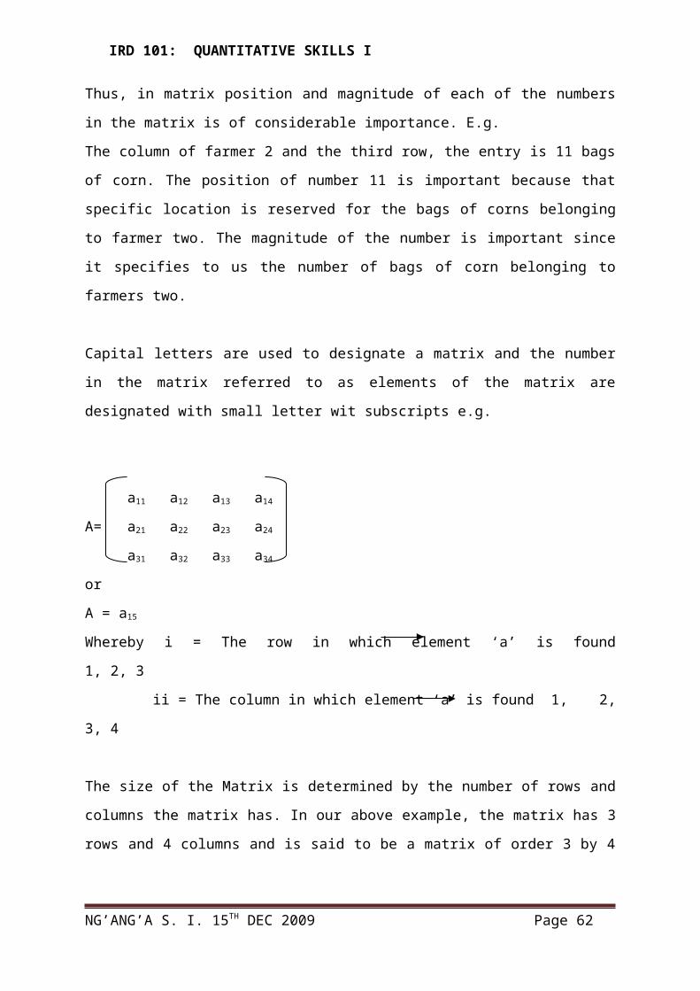
IRD 101: QUANTITATIVE SKILLS I
4.3.10 Inverse of a matrixInverse of a matrix, say A, and hence denoted by A-1 is given by adjoint of A divided by the
determinant of A. i.e.
A-1 = Provided that A is a non-singular matrix.
Example: Find the inverse of Matrix A defined as
6 -2 -3
A = -1 8 -7
4 -3 6
Solution:
/A/ = 293
27 -22 -29
Cof A = 21 48 10
38 45 46
27 21 38
Adj A = -22 48 45
-29 10 46
A-1 = = 27 21 38
-22 48 45
-29 10 46
=
NG’ANG’A S. I. 15TH DEC 2009 Page 62
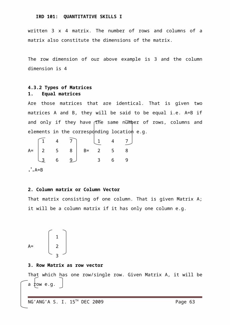
IRD 101: QUANTITATIVE SKILLS I
For a 2 x 2 matrix:
1. Interchange elements in main diagonal
2. Reverse the signs of element in the other diagonal
3. divide all elements by the determinant
Hence the inverse of A is
A = a b
c d
A-1 = a -d
-c a
NB: A-1 A = 1 0
0 1
Find the inverse of:
A = 2 2 ½ 5 -2 = 2.5 -1
4 5 -4 2 -2 1
Check 2 2 2.5 -1 = 1 0
4 5 -2 2 0 1
B= 2 -7 8 7 = -1.6 -1.4
-3 8 3 2 -0.6 -0.4
4.3.11 Solutions of Linear Simultaneous Equation by Matrix AlgebraConsider the following system of two linear equations with two variables.
a1 x1 + b1 x2 = Q1
a2 x1 + b2 x2 = Q2
NG’ANG’A S. I. 15TH DEC 2009 Page 63

IRD 101: QUANTITATIVE SKILLS I
Cramer’s rule can be used to get the values of X1 and X1 then the following expressions are
used.
X1 = Q1 b2 – Q2 b1 a1 b1 x1 = Q1
a1 b2 - b1 a2 a2 b2 x2 Q2
= Q1 b1
Q2 b2
a1 b1
a2 b2
X2 = a1 Q2 - a1 Q1
a1 b2 – b1 a2
= a1 Q1
a2 Q2
a1 b1
a2 b2
Suppose 1 P1 + 2 P2 = 1
1 P1 + 2 P2 = 2
By matrix algebra, it can be transformed to
1 2 P1 = 1
1 2 P2 2
Hence
P1 = 1 1
2 1 = 12 - 2 2
1 2 1 2 - 12
1 2
P2 1 1
1 2 = 12 - 1 1
1 2 1 2 - 12
1 2
NG’ANG’A S. I. 15TH DEC 2009 Page 64
Are two sentences equation Are two sentences equation - -
--
-
-

IRD 101: QUANTITATIVE SKILLS I
Example: Solve the following systems of linear simultaneous equations by matrix and inverse
methods
(i) 2x1 + 3x2 = 7 (ii) x1 + 2x2 + 3x3 = 3
x1 + 5x2 = 14 2x1 + 4x2 +5x3 = 4
3x1 + 5x2 + 6x3 = 8
Solutions
(i) 2 3 x1 = 7
1 5 x2 14
7 3
x1 = 14 5 = -7 = -1
2 3 7
1 5
X2 = 2 7
1 14 = 21 = 3
2 3 7
1 5
(ii) 1 2 3 x1 3
2 4 5 x2 = 4
3 5 6 x3 8
X1 3 2 3 1 2 3
4 4 5 2 4 4
8 5 6 = 7 X3 3 5 8 = 2
1 2 3 1 2 3
2 4 5 2 4 5
3 8 6 3 5 6
X2 = 1 3 3
2 4 5
NG’ANG’A S. I. 15TH DEC 2009 Page 65
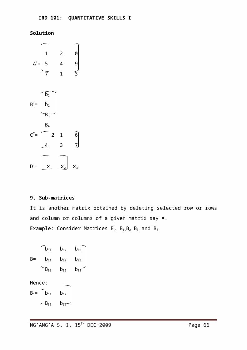
IRD 101: QUANTITATIVE SKILLS I
3 5 6 = -5
1 2 3
2 4 5
3 5 6
4.3.12 Solution of simultaneous equation by inverse method Given 3 simultaneous equation i.e.
a1 x1 + b1 x2 + c1 x3 = q then a1 b1 c1 x1 = q
a2 x1 + b2 x2 + c2 x3 = r a2 b2 c2 x2 r
a3 x1 + b3 x2 + c3 x2 = s a3 b3 c3 x3 s
a1 x1 + b1 x2 = q then a1 b1 x1 = q
a2 x1 + b2 x2 = r a2 b2 x2 r
Thus, A X = B Whereby
Hence solution of the equations by inverse method is given by
AX = B
Matrix rearranged – get the inverse of the given matrix by A-1 and multiply it on both sides,
hence:
A-1 A X = A-1B
X = A-1 B
Example
Find the solutions of the following equations by inverse method.
(i) 2x1 + 3x2 = 7 (ii) x1 + 2x2 + 3x3 = 3
x1 + 5x2 = 14 2x1 + 4x2 +5x3 = 4
3x1 + 5x2 + 6x3 = 8
Solution
(i) 2x1 + 3x2 = 7
x1 + 5x2 = 14
Step 1. Rewritten in the form of AX = B = 2 3 x1 = 7
1 5 x2 14
A X B
NG’ANG’A S. I. 15TH DEC 2009 Page 66
A X B
A X B
-1
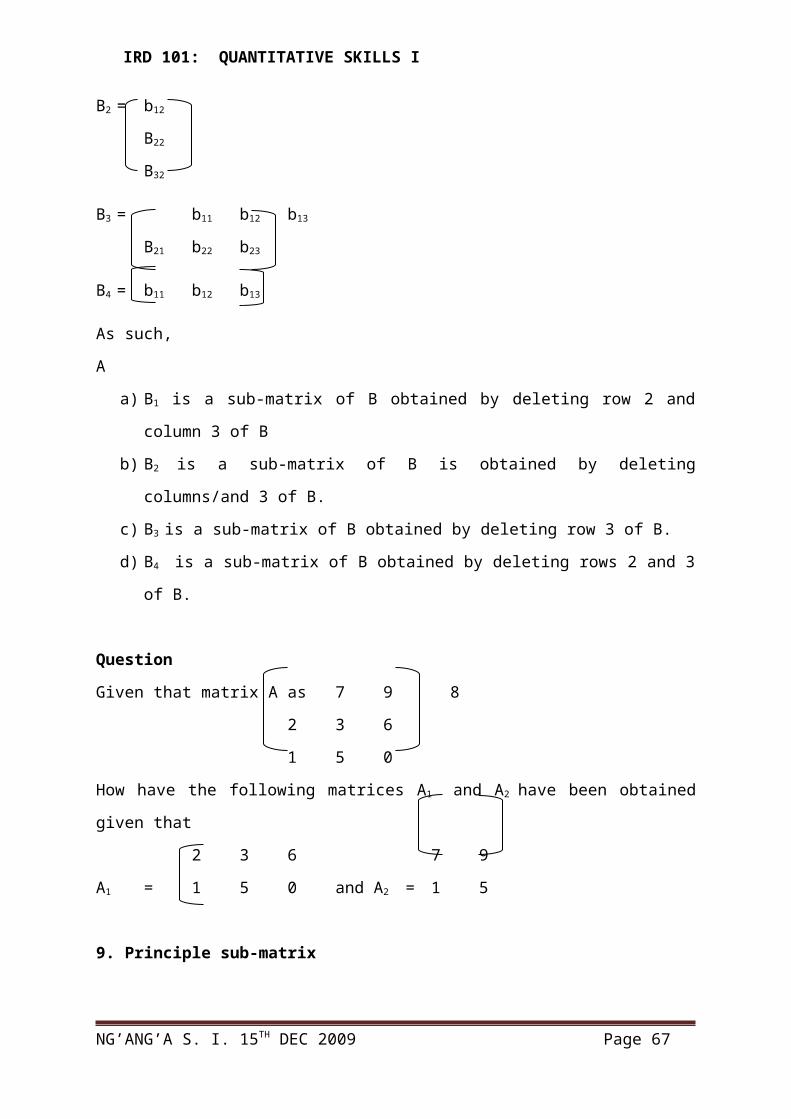
IRD 101: QUANTITATIVE SKILLS I
2. Get the inverse of the matrix hence.
2 3 2 3 x1 = 2 3 7
1 5 1 5 x2 1 5 14
x1 = 2 3 7
x2 1 5 14
7
14
= -1
3
(ii) x1 + 2x2 + 3x3 = 3
2x1 + 4x2 +5x3 = 4
3x1 + 5x2 + 6x3 = 8 Rewritten in the form of AX = B
1 2 3 x1 3
2 4 5 x2 = 4
3 5 6 x3 8
A X B
(ii) Get the inverse of A and multiply on both sides hence
Hence x1 =7, x2 = -5, and x3 = 2
4.3.13Revision Questions1. i) Given that A= find A-1
10mks
ii) Hence or otherwise solve the following system of simultaneous equations
6mks
2. if A=
NG’ANG’A S. I. 15TH DEC 2009 Page 67
-1-1-1
-1
-1-1-1

IRD 101: QUANTITATIVE SKILLS I
Findi.) 3(A-C) 3mks
ii.) B1A 2mksiii.) BC-B 3mks iv.) AC-C 3mksv.) AC1 3mks
b.) i.) Determine A-1, showing all the necessary workings 5mksii.) Hence or otherwise determine the solution to the following systems of equations 2x-y+3z=2-x-3y+z=-112x-2y+5z=3
5mks
3. Given matrix
Compute i.) BtA 2mksii.) AB 2mksiii.) What is the rank of matrix B 1mks
4. a)
b) Determine A-1, showing all necessary workers 12mksii) Hence or otherwise solve the following systems of simultaneous equations
5.
(a) If A = B =
Find (i) AT (1mark)(ii) BT (1mark)(iii) (2marks)(iv) (2marks)
(b) Solve by row operation or otherwise the simultaneous equations
(c). The relationship between Kenyan and Australian time is linear, such that if it is 7 am in Kenya, it is 8 p.m in Australia. When it is 4 p.m in Kenya it is 5 am in Australia.
i.) Write an equation to express Australian time in terms of Kenyan time. 3mksii.) What will be the time in Kenya if it is 2 p.m in Australia? 3mks
3. Solve for x, y and z using any method:
NG’ANG’A S. I. 15TH DEC 2009 Page 68
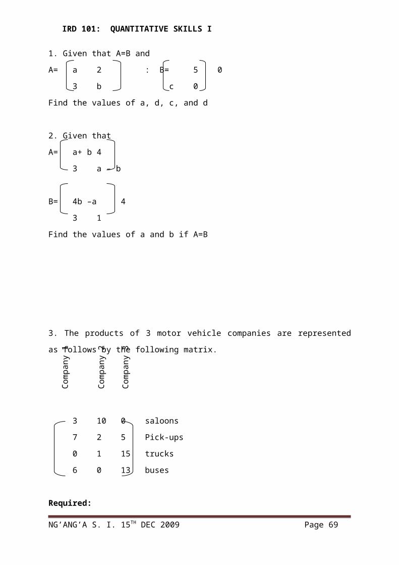
IRD 101: QUANTITATIVE SKILLS I
5.0 GRAPHS: (DATA PRESENTATION)
Introduction
Principles of Graph constructions
Types of Graphs and their uses
Construction of the Lorenz curve
Construction of z-curves
Construction of Semi-logarithm graphs
Revision questions
5.1 Introduction
Research data analysis, is followed, where necessary by a visual display of the data either in the form of a chart, table, graph or a diagram to facilitate communication with readers. The following section presents the various types of data presentation, visual display methods commonly used in research. A researcher will then choose the method of presentation that best presents the research data.
5.2Frequency distributionFrequency distribution presents data by dividing them into classes and recording the number of observation in each class. The number of classes in a frequency distribution is fixed somewhat arbitrary but there should be between five and twenty classes. A simple rule of the thumb is that (2c n) two raised to the number of classes (c) should be slightly more or equal to the number of observations (n). The range of values formed within each class called class interval (C.I) should be equal in all classes in a frequency distribution. The class interval (C.I) can be established by dividing the range (R) (Largest value – the smallest value) by the number of desired classes (C), So that:
C.I = R ?
C
The mid point (m) of each class is calculated by dividing the sum of the lower class boundary and the upper class boundary by 2.
Example A researcher has obtained the following data of the number of units of a product made per month by each of the fifty employees sampled form a manufacturing firm in Eldoret.Form a frequency distribution.
110 175 161 157 155 108 164 128 144 17842 30 62 158 156 167 124 164 146 116149 79 113 69 121 93 143 140 144 187165 147 184 133 104 197 195 141 40 103151 122 71 94 97 150 203 162 148 113
Solution
NG’ANG’A S. I. 15TH DEC 2009 Page 69
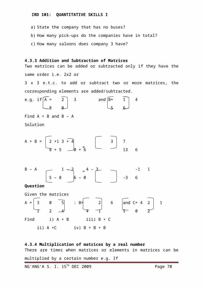
IRD 101: QUANTITATIVE SKILLS I
Step 1 - Numbers of classes necessary.2c 50 (number of respondents)When c – 6, 2c = 64 hence 6 would be appropriate number of classes.
Step 2 - Class intervals (C.I)C.I = R
C
R (Range) = 203 (highest number of units) – 30 (smallest number of units) = 173C = 6 C.I = 173 29
6
Step 3:- Forming the frequency distribution
Class Frequency30 – 5959 – 8788 – 116117 – 145 146 – 174 175 – 203
341010750
5.3 Cumulative Frequency DistributionThe cumulative frequency distribution used to determine the number of observations that are greater than or less than cumulative frequency distribution may be constructed as shown in example 4.2.2Example 4.2.2Construct less than and more than cumulative frequency distribution from the frequency distribution formed from data in example.
NG’ANG’A S. I. 15TH DEC 2009 Page 70
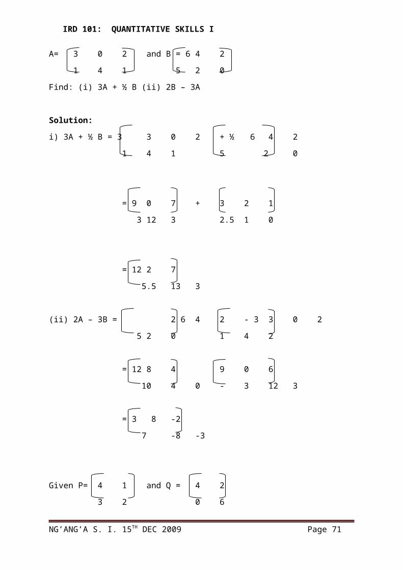
IRD 101: QUANTITATIVE SKILLS I
Less than cumulative frequency distribution (CFD)
Class Frequency (CFD)Less than 305988117 146 175204
0341010167
03717274350
More than cumulative frequency distribution (CFD)
Class Frequency (CFD)Less than 305887116 145 174203
50341010167
504743332370
5.4 OgiveAn ogive is a cumulative frequency distribution displayed pictorially. It could be a less than or more than ogive. To construct an ogive the limits of the class are plotted on the horizontal axis (abscissa) while the cumulative frequencies are plotted on the vertical axis (ordinate) of a Cartesian ordinate. Fig 1 shows a less than and fig. 2 a more than ogive constructed from data in example.
NG’ANG’A S. I. 15TH DEC 2009 Page 71

IRD 101: QUANTITATIVE SKILLS I
Example 4.2.3From data in example 4.2.1 and 4.2.2 construct a less than or more than ogive.
Fig 4.2.1 Less than Ogive
Graphs of Frequency Distributions:
The graphs of a frequency distribution of continuous type are as under –
(a) Ogive curve
(b) Histogram
(c) Frequency polygon
(d) Frequency curve
These are explained as under:-
Ogive Curve:
An Ogive is the name given to the curve obtained when the cumulative frequencies of a
distribution are graphed. It is also called cumulative frequency curve. The following steps
are adopted to construct an ogive: -
(i) Compute the cumulative frequency of the distribution.
NG’ANG’A S. I. 15TH DEC 2009 Page 72
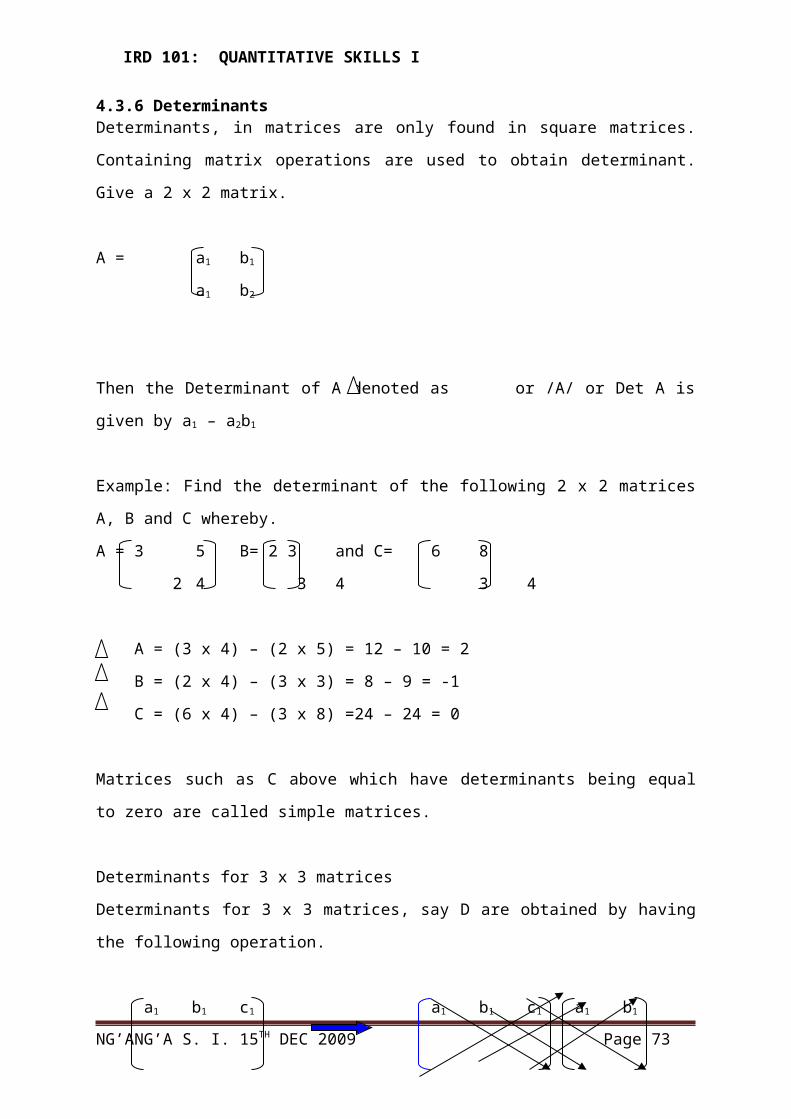
IRD 101: QUANTITATIVE SKILLS I
(ii) Prepare a graph with the cumulative frequency on the vertical axis and class
intervals on the horizontal axis,
(i) Plot a starting point at zero on the vertical scale and the lower class limit of the
first class.
(ii) Plot the cumulative frequencies on the graph at the upper class limits of the
classes to which they refer,
(iii) Then join all these points by the help of a curve
An ogive curve is used to find out the values of deciles and percentiles graphically
NG’ANG’A S. I. 15TH DEC 2009 Page 73

IRD 101: QUANTITATIVE SKILLS I
Example 9:
From the following information, draw an ogive curve:-
Class Frequency
0 – 10 5
10- 20 10
20 – 30 15
30 – 40 8
40 – 50 7
Solution:
To draw an ogive curve, the frequency is to be converted into cumulative frequency as
follows- cumulative
Class F c.f
0 – 10 5 5
10- 20 10 15
20 – 30 15 30
30 – 40 8 38
40 – 50 7 45
Mark cumulative frequencies (c.f.) on the graph paper, c.f of each group is marked against
upper limit of the respective group.
5.5 Relative frequency distribution A relative frequency distribution expresses the frequency within a class as percentage of the total number of observations in the sample as shown I example 4.2.4
NG’ANG’A S. I. 15TH DEC 2009 Page 74
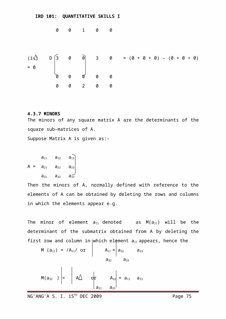
IRD 101: QUANTITATIVE SKILLS I
Example 4.2.4Prepare a relative frequency distribution from the frequency distribution of the factory workers in example 4.2.4
Class Frequency Relative frequency30-58
59-87
88-116
117-145
146-174
175-203
3
4
10
10
16
7
3 x 100 = 650
4 x 100 = 850
10 x 100 = 2050
10 x 100 = 2050
16 x 100 = 3250
7 x 100 = 1450
A cumulative relative frequency distribution can be generated in a similar way.
5.6 Histograms and bar chartsHistograms place the classes of a frequency distribution on the horizontal axis and the frequencies and the frequencies on the vertical axis. The area in each rectangular bar is proportional to the frequency in that class. Fig 4.2.4 shows the histogram of the data in example 4.2.1Fig. 4.2.4 Histogram of units of a product produced by factory workers.
5.7 Frequency polygonA frequency polygon expresses the distribution of data by means of a single line determined by the midpoints of the classes. It starts with the mid point of a class lower and ends with midpoint of a class higher than that data given as shown.
Fig. 4.2.5 Frequency polygon of units of a product produced by a factory worker
NG’ANG’A S. I. 15TH DEC 2009 Page 75

IRD 101: QUANTITATIVE SKILLS I
5.8 GraphsA graph is any pictorial representation of data where the Cartesian co-ordinates are used. The independent variable is shown on the x-axis and the dependent variable along the y-axis. A graph should have a clear and comprehensive title. It should be proportional with the horizontal and vertical scales chosen carefully so as to give the best possible appearance. The scales should accommodate the whole data and a false baseline may be used to avoid an unnecessarily elongated axis. The table from which the data used to plot the graph should be given alongside the graph and on index used to show the meaning of different curves used in a graph. If the data plotted is not original, than the source of data or information must be shown at the base of the graph.
Example 4.2.5 A researcher has obtained data on the total scales revenue and cost of production ABC Ltd Company shown below; plot a graph for the data.
Fig 4.2.6 ABC Ltd Total Revenue – Cost graph for the lasts six years
NG’ANG’A S. I. 15TH DEC 2009 Page 76
Year 1 2 3 4 5 6Cost of production (000) Sh 40 30 35 30 25 20Total Revenue (000) Sh 20 30 40 45 50 55
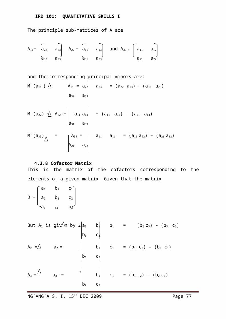
IRD 101: QUANTITATIVE SKILLS I
5.9Pie-ChartsA pie chart presents data in the form of a circle. The slices represent absolute or relative proportions. A pie chart is formed by making of a portion of the pie corresponding to each characteristic being displayed.
Example 4.2.6A researcher studying the distribution of manufacturing costs in ABC Ltd found that 20% of the firms unit cost is due to labour, 40% raw materials, 25% maintenance costs and 15% debt servicing. Present this information in a pie chart.Fig 4.2.7 A pie chart representing the distribution of ABC Ltd per unit manufacturing cost during the year.
5.8TablesThe table is the most commonly used in presenting statistical data. Tables are classified into general-purpose tables that are used for reference purposes. Examples of general-purpose tables are mathematical tables such as the normal distribution (Z) tables, logarithm tables and trigonometric tables. The other classification is the special purpose tables that provide information for particular discussion. All tables must contain the following parts;(i) Title
A title describes the content of a table and should indicate: - What - Data is included in the body.Where - Area covered in data collection.
How - Data is classified.
When - Data will apply (period)
(ii) Captions – These are headings at the top of the columns(iii) Stub – Describes the rows.(iv) Body – content or statistical data a table is designed to present.(v) Head Notes – Written above the captions and below the heading are used to
explain certain points relating to the whole table.(vi) Foot Notes – Placed below the stubs and are used to clarify some points included in
the table that is not explained in other parts.(vii) Source – Usually written below the footnotes and indicates where the content of the
table is obtained from if not originally collected.
NG’ANG’A S. I. 15TH DEC 2009 Page 77

IRD 101: QUANTITATIVE SKILLS I
There are two types of tables:(i) Simple or one-way table
This type of a table shows only one characteristic against which the frequency distribution is given.
Example 4.2.6
Table 4.2.7 frequency distribution of number of units produced per worker in ABC Ltd in 2003.
Class No of Units Produced
Frequency
30-58
59-87
88-116
117-145
146-174
175-203
3
4
10
10
16
7
(ii) Contingency Tables Two or more characteristics are shown in one table and indicate the number of observations for all variables that fall jointly in each category.
Example 4.2.7Table 4.2.8ABC workers level of salary and education and training in 2002
Level of Education and TrainingHigh Low
Level of Salary Earned
High 10 5Low 10 25Total 20 30
A good table should be attractive and manageable. It should make it possible or easy to make comparisons and should be prepared according to objectives. They should be prepared scientifically so as to be clear and easy to understand.Generally tables should be numbered, should not be over worded, should have figures rounded to avoid unnecessary details and should not be too narrow. All parts should be shown clearly with columns with figures to be compared close together. Units of measurements should be shown and all contents should be visible at a glance.
NG’ANG’A S. I. 15TH DEC 2009 Page 78

IRD 101: QUANTITATIVE SKILLS I
5.10Other DiagramsThere are other forms of visual presentation of statistical data that researcher may use to light basic facts and relationships, such as:-
-Scatterplots- Line diagrams-Two Dimensional diagrams- Three dimensional diagrams- Pictograms and - Cartogram
These are illustrated in fig 4.2.9* * * Y* * * ** *
X XScatter plot/graph Line diagramY
X
Two dimensional diagram
Cartogram Key wet lands ……….. Semi arid lands Dry land
NG’ANG’A S. I. 15TH DEC 2009 Page 79

IRD 101: QUANTITATIVE SKILLS I
0
20
40
60
80
100
1st qt 2nd qt 3rd qt 4th qt
Series1
Series2Series3
Three dimension diagramsIt would be worthwhile to be conversant with all of them so as to add them to the variety of choice when deciding on how to present research data.It cannot be over- emphasized that visual display of research data breaks monotony, attracts and captures readers’ attention and adds quality to the presentation of research data.
NG’ANG’A S. I. 15TH DEC 2009 Page 80
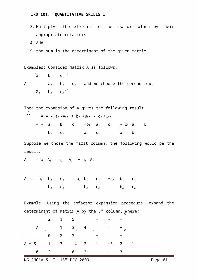
IRD 101: QUANTITATIVE SKILLS I
5.11 SPECIAL TYPES OF GRAPHS The following are the important types of graphs;-
1. Time series graphs or histogram (This is discussed on its own under topic 7).
2. Z – charts
3. Scattergraphs
4. Semi-logarithmic graphs or ration scale graphs
5. Lorenz curve
6. Graphs of frequency distribution
These graphs are explained as under
5.11.1 Z Charts A Z chart is simply a time series chart incorporating three curves for
(i) Individual monthly figures.
(ii) Monthly cumulative figures for the year
(iii) A moving annual total.
Z chart takes its name from the fact that the three curves together tend to look like the letter
Z.
A Z chart is of great importance for presenting business data over a period of one year. The
information given in a Z chart can be explained under.
(i) Monthly totals – These simply show the monthly results at a glance together with
any rising or falling trends and seasonal variations.
(ii) Cumulative totals – These show the performance to date and can be easily
compared with planned or budgeted performance.
(iii) Annual moving totals – these show comparison of the current levels of
performance with those of the previous year If the line is rising then this year's
monthly results are better than the results of the corresponding month last year
and vice versa.
Sometimes, separate vertical scales are used to plot the monthly data and the data for the
cumulative and the moving annual totals In some cases, the same vertical scale is used to plot
the monthly data and the data for the cumulative and the moving annual totals The decision to
take same vertical scale or separate vertical scales should be made in view of the nature of the
given data.
NG’ANG’A S. I. 15TH DEC 2009 Page 81
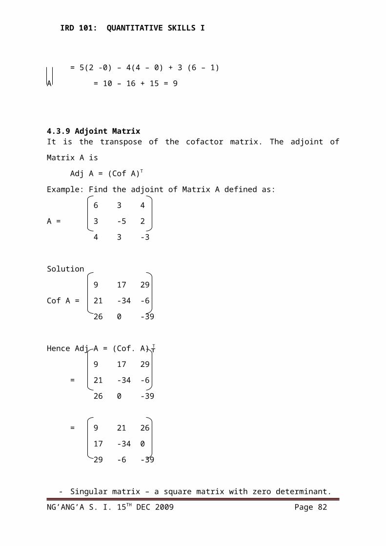
IRD 101: QUANTITATIVE SKILLS I
Example 5:
The following are the sales of ABC Ltd for the years 1995 and 1996
1995 1996
January 400 420
February 480 450
March 420 600
April 580 640
May 600 580
June 800 700
July 750 800
August 600 750
September 550 600
October 500 480
November 600 550
December 900 950
(Source)
Construct a Z chart for the year 1996.
NG’ANG’A S. I. 15TH DEC 2009 Page 82

IRD 101: QUANTITATIVE SKILLS I
Solution
Z Chart of sales 1996
1995 1996
Monthly
cumulative
for 1996
Moving
annual
Total
January 400 420 420 7200
February 480 450 870 7170
March 420 600 1470 7350
April 580 640 2110 7410
May 600 580 2690 7390
June 800 700 3390 7290
July 750 800 4190 7340
August 600 750 4940 7490
September 550 600 5540 7540
October 500 480 6020 7520
November 600 550 6570 7470
December 900 950 7520 7520
7180 7520
Monthly cumulative totals are obtained as under;-
February = 420 + 450 = 870
March = 870 + 600 = 1470
April = 1470 + 640 = 2110 and so on
Moving annual totals are obtained as under:-
January = 7180 + 420 – 400 = 7200
February = 7200 + 450 – 480 = 7170
March = 7170 + 600 – 420 = 7350 and so on.
NG’ANG’A S. I. 15TH DEC 2009 Page 83

IRD 101: QUANTITATIVE SKILLS I
It can be observed that the moving annual totals ran be easily obtained by adding the current
month's figure and subtracting the corresponding last year's figure to and from the preceding
month's annual total In this example, the total sales of 1995 are 7180. In order to obtajin the
moving annual total at the end of January 1996, add January 1996's sales into 7180 and
subtract from it. the sales of January 1995.
The chart is constructed below -Y
5.11.2 Scatter GraphsScatter graphs are those graphs which are used to indicate the relationship between two
variables. The X-axis is used to represent the data of one variable and the Y-axis to represent
the data of other variable.
In order to construct a scatter graph or scatter diagram, we must have several pairs of two
variables. Each pair of these variables shows the value of one variable and the corresponding
value of the other variable. Each pair of data is plotted on a graph. The resulting graph will
show a number of plotted pairs of data scattered over the graph.
Scartergraphs are usually drawn to indicate the relationship between two variables. For this
purpose, a line of best fit is established from the scatter graph.
The line of best fit is that line from which the total deviation of the points plotted on a scatter
diagram is minimum. The line of best fit indicates the relation or association between two
NG’ANG’A S. I. 15TH DEC 2009 Page 84

IRD 101: QUANTITATIVE SKILLS I
variables. It is one way of measuring correlation. In a scatter graph, the line of best fit is
drawn approximately. This line may have a rising or felling trend which shows positive and
negative relationship between two variables respectively.
Example 6: Sales and advertising expenditure of RST Ltd are given below for a period of
seven months.
Advertising expenditure (Sh 000’s)
20 25 30 35 40 45 50
Sales (Sh 000’s)
650 550 700 800 750 900 850
Draw a scatter graph
Solution
in this example, the advertising expenditure is taken along – axis because it is independent
variable and sales are taken along Y – axis as these are dependent variable.
It can be observed from the graph that the plotted data, although scattered represent the rising
trend. It means the increase in advertising expenditure results in higher sales. This trend
shows there is a positive relationship between these two variables.
NG’ANG’A S. I. 15TH DEC 2009 Page 85

IRD 101: QUANTITATIVE SKILLS I
5.11.3 Semi - logarithmic graphs:A semi-logarithmic graphs is that graph on which the vertical scale is logarithmic. It is also
known as ratio scale graph. These graphs are useful to study the relative movements instead
of absolute movements.
Semi-logarithmic graphs are generally used when:-
1. Visual comparisons are to be made between series of greatly different magnitudes.
2. The series are quoted in non-comparable units.
3. The data are to be examined to see whether they are characterised by a constant rate
of change. A constant rate of change appears as straight line.
Ratio scale or semi-log graphs can be constructed in three ways:-
1. By using semi-log graphpaper
2. By using a slide rule
3. By plotting the logs of the variables.
Actual values can also be shown on the vertical scale. Zero has no log and Zero' should not
be inserted on the vertical scale of a semi-log graph.
In semi-log graphs, the horizontal scale is the same as on ordinary graph whereas the vertical
scale is the ratio scale or logarithmic values of the variable.
If the logarithmic curve is moving upward, it indicates that the rate of growth is increasing
and vice versa. If such a curve is a straight line, it means the rate of growth is constant.
NG’ANG’A S. I. 15TH DEC 2009 Page 86

IRD 101: QUANTITATIVE SKILLS I
Example 7:
The following are the profits of Pombe Breweries Ltd over the calendar year 1996.
Month Profits in '000' of Shillings
January 10February 11March 13April 15May 15June 18July 16September 19August 20October 17November 18December 24
Using the ordinary graph paper, plot the time series for the profits using the logarithmic
values or ratio scale
Month Profits (Sh. 000’s) Logy
January 10 4.0
February 11 4.0
March 13 4.1
April 15 4.2
May 15 4.2
June 18 4.3
July 16 4.3
September 19 4.3
August 20 4.3
October 17 4.2
November 18 4.3
December 24 4.4
Note: Profit for January is Shs. 10,000 so the characteristics are 4 and so on.
NG’ANG’A S. I. 15TH DEC 2009 Page 87

IRD 101: QUANTITATIVE SKILLS I
In a semi-logarithmic graph, one axis has a logarithmic scale and the other axis has a linear
scale.
Example 1: Variable Exponent
Plot the graph of y = 5x on normal and then semi-logarithmic paper.
Answer:
We first graph y = 5x using ordinary x- and y- linear scales (the space between each unit
remains fixed for both axes):
We see that the detail for anything less than x = 2 is lost.
Using a semi-logarithmic scale on the y axis gives:
NG’ANG’A S. I. 15TH DEC 2009 Page 88

IRD 101: QUANTITATIVE SKILLS I
We can now see much more detail in the y values when x < 2.
Notice that the numbers along the x axis are evenly spaced, while along the y-axis, we have
powers of 10 evenly spaced.
Example 2: Variable Raised to a Fractional Exponent
Let's now graph y = x1/2 using all 3 axis types. This function is equivalent to y = √x.
Using rectangular axes, we can see that the graph of y = x1/2 is half of a parabola on its side
(i.e. its axis is vertical):
NG’ANG’A S. I. 15TH DEC 2009 Page 89

IRD 101: QUANTITATIVE SKILLS I
We have seen this curve before, in The Parabola section.
Note 1: The detail near (0, 0) is not so good using a rectangular grid.
Note 2: The curve passes through (0, 0), (1, 1), (4, 2) and (9, 3). In each case, the y-value is
the square root of the x-value, which is to be expected.
Let's see the curve using a semi-logarithmic plot.
Now we have a lot better detail for small x. The lowest value of y that the graph indicates is y
= 0.1. We cannot show y = 0, since the logarithm of 0 is not defined.
We can see that the curve still passes through (1, 1), (4, 2) and (9, 3).
Application 1: Air pressure
1. By pumping, the air pressure in a tank is reduced by 18% each second. So the percentage
of air pressure remaining is given by p = 100(0.82)t.
Plot p against t for 0 < t < 30 s on
(a) A rectangular co-ordinate system
(b) A semi-logarithmic system.
NG’ANG’A S. I. 15TH DEC 2009 Page 90

IRD 101: QUANTITATIVE SKILLS I
Try it on paper first, and then see what you get using the LiveMath example above.
The answer is given below.
Answer:
(a) Rectangular plot:
(b) Semi-logarithmic Plot:
5.11.4 LORENZ CURVE
NG’ANG’A S. I. 15TH DEC 2009 Page 91
IRD 101: QUANTITATIVE SKILLS I
This is a graph to measure dispersion. It was devised by Dr. Lorenz to measure inequalities of
wealth distribution. So an important use of the Loren curve is in the measurement of the
extent to which income is unevenly distributed between the various income groups. The
disparity of proportions is a common economic phenomenon. This disparity can be
demonstrated by the help of Loren curve
A Lorenz curve is constructed as follows:-
1. Write down the values of the two variables being plotted
2. Express the variables as percentages of the total.
3. Compute the cumulative percentages of each variable.
4. Draw a horizontal and vertical axis and plot 0% to 100°o on .-.-u ii axis
5. Mark the cumulative percentages on the graph and join the points together by a free
hand curve. This is Lorenz curve.
6. Draw the line of equal distribution by joining 0% to the 1000 point by a straight line.
If the Lorenz curve is away from the line of equal distribution, there is greater disparity or
inequality and vice versa.
Example 8:
The following figures are taken from surrey on "Business Prospects" for 1996
Maize Flour Sales
Number of Establishment s Net output(£'000')
23
26
24
19
14
6
104
450
860
1350
2190
3125
Draw a Lorenz Curve using the above data.
Solution:
Maize Flour Sales
Net output (£ ‘000’)
NG’ANG’A S. I. 15TH DEC 2009 Page 92

IRD 101: QUANTITATIVE SKILLS I
Number of
establishments
% Cumulative
104
450
860
1350
2190
2125
8079
% Cumulative
23
26
24
19
14
6
20.5
23.2
21.4
17.0
12.5
5.4
20.5
43.7
65.1
82.1
94.6
100.0
1.3
5.6
10.6
16.7
27.1
38.7
1.3
6.9
17.5
34.2
61.3
100.0
112 100.0 100.0
This curve shows the greater disparity between the numbers of establishments and the net
output 20.5% establishments have only 1.3% net output and 5.4% establishments have 38.7%
share of net output.
The Lorenz curve is a graphical device used to demonstrate the equity of distribution of a
given variable such as income, asset ownership or wealth. For example, one might be
interested in the equity of cattle ownership since this is often taken as an indicator of the
NG’ANG’A S. I. 15TH DEC 2009 Page 93
0
Line of Equal Distribution
0
20
40
60
80
100
Y
20 40 60 80 100X
Lorenz Curve
Number of establishment
IRD 101: QUANTITATIVE SKILLS I
distribution of wealth, particularly for pastoral and agropastoral societies. The distribution of
cattle ownership is, however, often extremely difficult to determine so that the cattle holding
per household (or per holder) is often used as the proxy measure of wealth in the derivation
of a Lorenz curve. Holding implies the right and responsibility to manage on a day-to-day
basis but not necessarily to dispose of (e.g. by slaughter, sale or gift).
A graph for showing the concentration of ownership of economic quantities such as wealth
and income; it is formed by plotting the cumulative distribution of the amount of the variable
concerned against the cumulative frequency distribution of the individuals possessing the
amount.
A cumulative frequency curve showing the distribution of a variable such as population
against an independent variable such as income or area settled. If the distribution of the
dependent variable is equal, the plot will show as a straight, 45° line. Unequal distributions
will yield a curve. The gap between this curve and the 45° line is the inequality gap. Such a
gap exists everywhere, although the degree of inequality varies
In the following example, a Lorenz curve for cattle holdings to households holding cattle is
therefore constructed. The principles outlined in the derivation of the curve can be applied to
any data set in which the equity of distribution for a given variable is being calculated.
Derivation of the Lorenz curve
In the derivation of the example Lorenz curve, the following procedure has been adopted:
All individual units (households) are ranked from the lowest to the highest according
to the number of cattle held (Column 1, Table 2.A1) and the number of households in
each cattle-holding category is given (Column 2).
From this data, the percentage of households falling into each cattle-holder category is
derived (Column 3).
The cumulative percentage of households in each cattle-holder category is then
estimated (Column 4).
NG’ANG’A S. I. 15TH DEC 2009 Page 94

IRD 101: QUANTITATIVE SKILLS I
By multiplying the number of cattle in each category by the number of households
holding those cattle (Column 1 x Column 2), we then obtain the total number of cattle
held within each category (Column 5).
From this latter figure, the percentage of total cattle held (Column 6) and the
cumulative per cent of cattle held in each category (Column 7) are obtained.
The cumulative percentage of cattle held in each category (vertical axis) is then
plotted against the cumulative percentage of households for each category (horizontal
axis) to derive the Lorenz curve (Figure 2A.1).
This plotted curve is then compared with the line of perfect equity (drawn at 45° from
the origin of the graph) to provide an indication of the equity of distribution of cattle
holdings within the area concerned.
5.12Revision questions1. A hypothetical research on the average width of maize leaf in mm against the amount of calcium potassium nitrate fertilizer applied in grammes yielded the following results.Width of maize leaves (in mm) Fertilizer in grams 20.020.521.021.522.022.523.023.524.024.5
19161817181914121111
Required i.) using semi average method constructs a graph for the information above 6mks ii.) using the graph in i.) Estimate the size of maize leaf when you apply 8 grams of the fertilizer. iii.) Assume the graph depicts a true situation, what will be your comment to the use of this fertilizer with respect to the size of maize leaf?2. The following represents the earnings period in shillings of 50 casual workers of a certain company.211 215 230 234 261270 291 294 244 239286 275 266 268 221216 259 232 212 211
NG’ANG’A S. I. 15TH DEC 2009 Page 95

IRD 101: QUANTITATIVE SKILLS I
290 246 229 250 254265 272 273 280 261218 219 238 225 240246 257 231 263 241268 274 271 270 267276 447 248 254 257
a.) using the size of 8 shilling and beginning with 211-218 classi.) form a frequency distribution 4mksii.) Construct a histogram and use it to estimate the modal earnings peer day 6mksiii.) graphically and not otherwise determine the median earnings per day 8mks
3. The annual DAP fertilizer consumption in thousands of tonnes during 1995-2001 in Lukuyani Division was recorded as given below.Year 1995 1996 1997 1998 1999 2000 2001Consumption (‘000) tonnes
50 56 60 68 70 75 78
a.) i.) Use the semi average method to fit the trend line and use it to estimate the consumption in 2005. 12mksii.) Indicate two major disadvantages of this method 4mksb.) Construct semi logarithmic graph for the consumption of the Lukuyani and use it to [comment on the rate of consumption. 8mks
4. The table shows the number of workers employed in two institutions REK and PEDI respectively with regards to salaries paid to them in the year 2005.REK PEDINumber of workers Salaries and
allowances Number of workers Salaries and
allowances60 2800 80 420070 4900 50 510055 6400 45 660050 7700 35 880040 8400 28 1060020 6800 23 1230010 5000 16 100005 4000 4 5000
i. Construct on the same graph Lorenz curve for the two institutions, round off your figure to nearest whole number 10mks
ii. Using Lorenz curve estimate iii. The production of salaries and allowances paid to the first 40% of workers in REK and
PEDI 4mksiv. The proportion of salaries and allowances paid to the last 10% of the top cream workers
in the two institutions.Join the origin ad the end point of Lorenz curves with a straight line, explain the importance
of the line with regards to income of workers with a view to pointing out the company with
better income distribution
5. a.) i.) Describe the advantages of using a graph as a means of data presentation 3mks ii.) Distinguish between frequency distribution and frequency polygon 2mks
NG’ANG’A S. I. 15TH DEC 2009 Page 96

IRD 101: QUANTITATIVE SKILLS I
iii.) Identify the differences between measures of central tendency and measure of variability 4mks
b.) The following information about the salaries of employees was obtained from a private company in agricultural sector in Kitale.
Salary Per Month X (Ksh) Frequency (f) 0-4000 94000-8000 368000-12000 9112000-16000 14716000-20000 8720000-24000 2224000-28000 8Required
i. Draw on the same axes a “less than” and an “or more” ogives 6mksii. Using the ogives find the median salary 2mks
iii. Calculate the most frequently occurring salary 2mksiv. Determine the mean and standard deviation of salary at the firm and describe the
distribution 5mks
6. In estimating the value of a plantation of cedar trees, the diameters of trees in a sample area of 100 trees were measured in centimeters and recorded as follows;14 5 7 8 5 18 4 15 8 149 8 11 14 9 14 18 15 13 1619 11 19 12 11 9 14 17 7 1513 17 14 18 16 12 5 11 15 1910 7 16 6 16 8 18 9 17 1014 8 6 19 13 16 16 15 10 117 6 19 16 9 9 8 17 13 910 12 14 4 14 7 14 18 5 107 11 18 9 11 10 15 13 18 1712 13 17 19 16 6 4 15 18 13
Required a.) Construct a histograph for the distribution and use it to estimate the modal size of the
diameter of the trees in the sample 6mksb.) Using the class size width of 3cm, limit inclusive, form a frequency distribution table
for the diameter of cedar trees starting from 4cm. 6mksc.) Form a cumulative frequency distribution of the diameter of the trees and construct a
more than ogive and use it to obtain the median 7mksd.) Determine the quartile deviation of the distribution 5mks
7. The table below gives the production figures (in 000 of tonnes) of ceramic goods for 2006. Month Jan Feb Mar Apr May Jun July Aug Sep Oct Nov Dec Production 335 325 310 354 360 338 333 270 375 395 415 373
i.) Plot the monthly production figures on a graph 5mks
NG’ANG’A S. I. 15TH DEC 2009 Page 97

IRD 101: QUANTITATIVE SKILLS I
ii.) Which time series factor seems to influence the production of ceramic goods? 3mks
iii.) Use the graph to estimate the production figures for the ceramic good in February 2007. 4mks
8. In order to observe patterns and trends, data are often presented in the form of charts. Discuss the type of chart that could be used in each case when it is relevant to use each type. (20 marks)9. State the points to be considered in the presentation of research data. (4 marks)
Explain with the aid of an example when and where each of the following may be used in the presentation of research data.Pie chart (4 marks)Ogive (4 marks)Bar chart (4 marks)Scatter diagrams (4 marks)
10. The table below shows the frequency distribution of daily income earned in 1991 by a sample of 50 workers of ABC Construction Company.
INCOMES NUMBER OF WORKERSKSHS50-54 255-59 360-64 565-69 1070-74 1275-79 880 - 84 685 – 89 390 – 94 1
REQUIREDUsing the graph paper to:
i Construct a histogram and frequency polygon. ( 8 marks)iiConstruct a cumulative relative frequency polygon (8 marks) Graphically determine; iii The sample median
(2 marks)iv The sample first quartile
(2 marks)
NG’ANG’A S. I. 15TH DEC 2009 Page 98
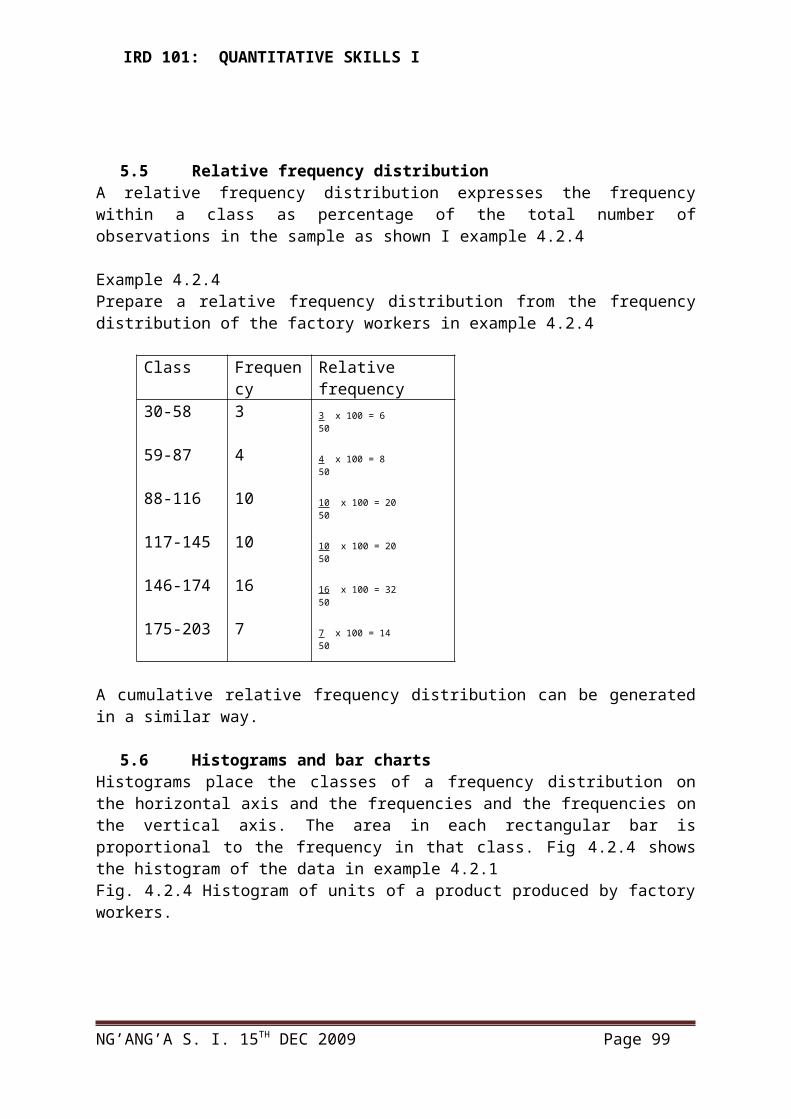
IRD 101: QUANTITATIVE SKILLS I
6 FREQUENCY DISTRIBUTION: (12 HOURS)
Methods of Data collection,
Frequency Tables, Polygons and curves
Measures of Central Tendency
- Mode, mean and median (mention others too)
Measures of Dispersion
Range, Standard Deviation, Quartile Deviation, Variance.
Bivariate Data
6.1Sampling and sampling design
6.1.1 SamplingSampling is taking any portion or universe as represented of that population or universe.
Sample: just a part of the population selected according to some rule or plan.Population: The totality of all possible values (measures, counts, or respondents) of a particular characteristic for a specified group of objects.
Sampling means selecting a given number of subjects from a defined as representative of that population or taking any portion of the universe as representative of that population or universe. One type of population distinguished by researchers is called the target population or universe- this means that all members of a real or hypothetical set of people, events or objects to which results of a research are generalized.
Sample: a sample is a small proportion of a population selected for observation and analysis, by observing the characteristics of a sample, one can make certain inferences about the characteristics of the population from which it is drawn, and samples are chosen in a systematic random way, so that chances or the operations of probabilities can be utilized. Therefore a sample is a part of population selected according to some rule of plan.
The section of such a sample and collection of data from it would involve a tremendous amount of work and expense. Instead a researcher must visually draw his sample from an experimentally acceptable population such as all form three students in district schools. If the researcher can demonstrate that the accessible population is closely comparable to the target population of a few variables that appear most relevant he or she has done much to establish population is reasonably representative of the target population.
Criteria of population validity
The criteria used to evaluate a sample of 460 articles in the field of marketing research are-
NG’ANG’A S. I. 15TH DEC 2009 Page 99

IRD 101: QUANTITATIVE SKILLS I
1. A Clear descriptions of the population to which the results are to be generalized are given.
2. The sampling procedure should be specified in enough details so as another investigator would be able to replicate the procedure. This should include at a minimum (a) the type of sample (b) sample size and (c) geographical area. In most educational studies other descriptive data, such as sex, age, grade level and social economic status should also be included.
3. The sampling frame. That is, the list, indexes, or other population records from which the sample was selected should be identified.
4. The completion rate – this is the proposition of the sample that participated as intended in all the research procedures should be given.
Random does not mean haphazard section. What it does mean is that each member of the population has some calculable chance of being selected- not always an equal chance. It also means the converse that there is no identified population who could not be selected when the sample is set up.
Why sample?Reasons for sampling include;
a. The population may be to large for complete enumeration.b. The enumeration or measurement process may be destructivec. Sample saves time and moneyd. Sampling allows more time to be spent on training, testing and checking.
N.B. the larger the sample the larger the potential level of confidence.
Sampling errorErrors due to inherent characteristics of the sampling procedure itself. Marked by the difference between the sample estimates and the population parameters under study. Most notable sampling errors are bias- the intuitional or systematic over or under – representation of the qualities of interest.
Non- sampling errorOccur whether or not complete enumeration or sample remunerations is adopted. They arise from failure to measure a certain phenomena, faulty questionnaire or ignorance. N.B. sampling errors decrease with increase in sample size while error increase with increase in sample size.
Reducing errorsTo reduce errors, all of the following strategies must be adopted;
i. Proper demarcations and identification of variables.ii. Suitable instruments.iii. Clear definition of conceptsiv. Pre-testing of instrumentsv. Use of expert enumerationvi. Close supervision of enumerators
Methods of accessing and controlling non- sampling errors
NG’ANG’A S. I. 15TH DEC 2009 Page 100
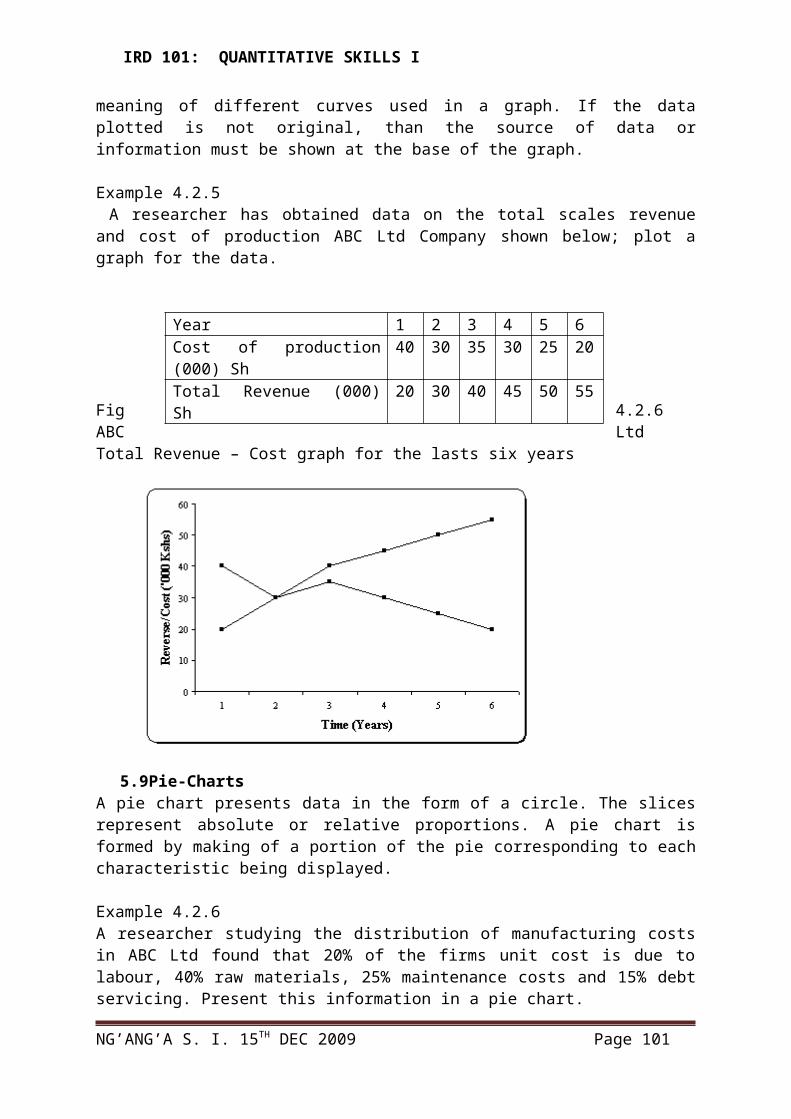
IRD 101: QUANTITATIVE SKILLS I
i. Check ups of the instrumentsii. Inter- penetrating samples iii. Post census or post sample surveyiv. Tracing techniquesv. Quality controls or instant checksvi. Study or recall lapsevii. Treatment of non- response cases.
Steps in sampling designWhile developing a sampling design, the researcher must pay attention to the following points:
a. Types of universe: the first step in developing any sample is to clearly define the set objective technically called the universe, to be studied. The universe can be finite or infinite. In finite universe the number of items is certain, but in the case of an infinite universe the number of items is infinite.
b. Sampling units: a decision has to be taken concerning a sampling unit before selecting samples. Sampling units may be a geographical one such as state, district and village.
c. Source list: it is also known as ‘sampling frame’ from which sample is to be drawn. It contains the names of all items of a universe (in case of finite universe only). If source list is not available, researcher has to prepare it. it is extremely important for the source list to be as representative population as possible.
d. Size of sample: this refers to the number of items to be selected from the universe to constitute a sample. This is a major problem before a researcher. The size of sample should neither be excessively large, nor too small. It should be optimal.
e. Parameter of interest: in determining sample decisions, one must consider the question of specific population parameter, which are of interest. for instance we may be interested on estimating the proportion of person with some characteristic in a population, or we may be interested in knowing some average or the other measure concerning the population.
f. Budgetary constraints: Cost considerations, from practical point of view, have major impact upon decisions relating to not only the size of the sample but also to the type of sample. This fact can even lead to the use of non-probability sample.
g. Sampling procedures: finally the researcher must decide about the technique to be used in selecting the items for the sample.
Criteria for selecting a sampling procedure in this context one must remember that two costs are involved in a sampling analysis viz., the cost of collecting the data and the cost of an incorrect inference resulting from the data researcher must keep in view two causes of incorrect inferences viz., systematic bias and sampling errors a systematic bias result from errors in sampling procedures, and it cannot be reduced or eliminated by increasing the sample size. At best the causes responsible for these errors can be detected and corrected. Usually a systematic bias is the result of one or more of the following factors.
a. Inappropriate sampling frame: if the sampling frame is inappropriate i.e. bias representation of the universe, it will result in a systematic bias.
NG’ANG’A S. I. 15TH DEC 2009 Page 101
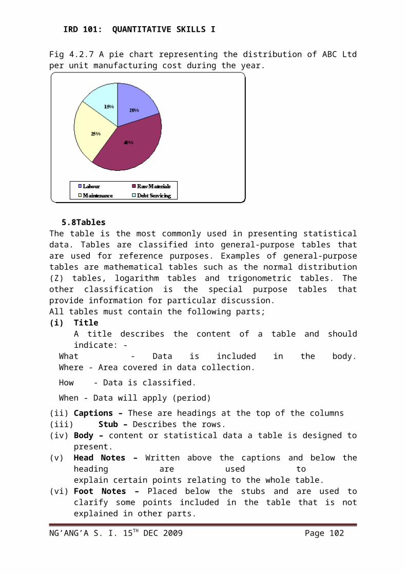
IRD 101: QUANTITATIVE SKILLS I
b. Defective measuring device: if the measuring device is constantly in error, it will result in systematic bias. In survey work systemic bias can result if the questionnaire or the interviewer is biased. Similarly, if the physical measuring device is defective there will be systematic bias in the data collected through such measuring device.
c. Non respondent: if we are unable to sample all the individuals initially included in the sample, there may raise a systematic bias.
d. Indeterminacy principal: some times we find that individuals act differently when kept under observation than what they do when they are kept in non- observed situations.Natural bias in the reporting of data: this is often the cause of a systematic bias in many inquiries. There is usually a downward bias of data collected by government taxation department. Whereas, we find an upward bias in the income data collected by social organizations. People generally understate there income if asked about it for tax purposes, but they overstate the same if asked for social status or affluence.
Types of samplesThere two types:
1. probability sample2. non- probability (purposive) sample
Probability samplesIn probability sampling, each element of the large population has a known probability of being selected. There are several ways of drawing probability samples, as follows;(NB: each element has an equal chance of being selected)
Simple random sample: the individual observation or individuals are chosen in such a way that each has an equal chance of being selected and each choice is independent on any other choice. If we wished to draw a sample of 50 individuals from a population of 600 names in a container and, blind folded draw one name at a time until the sample of 50 was selected. This procedure is cumbersome and rarely used.
Random numbers: a more convenient way of selecting a random sample or assigning individuals to experimental and control groups so that they are equated by use of a table of random numbers as shown below
Typical Table of Random NumbersRow 1 2 3 4 5 6 7 8 9 1012345678910
32388053006652344167479146344589917926482097981959
52390221644413364486052841736115665454540450865642
16815243690069764758376806282552872095526453574240
69298542243555275366208013990873823888153135556306
82732359833597076554721520560773144165338606400033
38480196871912431606393399128488662511252947267107
73817110526331812614348066883388970793754768977510
32523914912968633072089302557074492975960597470625
41961603830338760332850013881851805162965246828725
44437197465984692325878204692099378660921683434191
The use of random number tables, the researcher randomly selects a row or a column. If more numbers are needed he proceeds to the next row or column until enough numbers have been selected to make up the desired sample size. In effect the research may start at any random pointing the table and select numbers from a column or row as she wishes.
NG’ANG’A S. I. 15TH DEC 2009 Page 102

IRD 101: QUANTITATIVE SKILLS I
Systematic sampling: it is the way of selecting every nth item on the list. An element of randomness is introduced into this kind of sampling by using random numbers to pick up the nth item from which to start. For instance, if a four- percent sample is desired, the first item would be selected randomly from twenty- five and thereafter every twenty fifth item would be automatically be included in the sample. Thus in this sampling only the first unit is selected randomly and the remaining units of the sample are selected at fixed intervals.
Stratified sampling: under this the population is divided into several sub-group populations that are individually more homogeneous than the total population (the different sub- populations are called ‘strata’) and then we select items from each stratum to constitute a sample. Since each stratum is more homogeneous than the total population, we are able to get more precise estimates for each stratum and by estimating more accurately each of the component part we get a better estimate of the whole in brief stratified sampling results in more reliable and detailed information. The following question should be addressed in using stratified sampling: How should the strata be formed? (for example, it can be formed from the common characteristics of the items to be put in each stratum)How should items be selected from each stratum? (We can use simple random sampling or systematic sampling can be used in certain situations)How many items should be selected from each stratum or what is the sample size to each stratum? (The method of proportional allocation under which the sizes of the sample from different stratum are kept proportional to the size of the stratum is used)
Cluster sampling: if the total area of interest happens to be a big one, a convenient way in which a sample can be taken is to divide the area into a number of smaller non overlapping areas. Then, to randomly select a number of these randomly selected areas (usually called clusters), with the ultimate sample consisting of all (or sample of) units in this smaller areas or clusters. The respondents have heterogeneous characteristics in each cluster.
Area sampling: if clusters happen to be more geographical sub-divisions, cluster sampling is better known as area sampling. In other words, cluster design where the primary sampling unit represents a cluster of units based on geographical area sampling.
Multi- stage sampling: it is a further development of the principal of cluster sampling. Supposed we want to find out the performance of the English subject in district school. The first stage is to select large primary sampling unit – a district. Then we may select certain divisions then interview all selected subjects in the division. This would represent a two stage sampling design with the ultimate sampling unit being clusters of divisions.
Sampling with probability proportional to size: incase the cluster sampling unit do not have the same number or approximately the same number of elements, it is considered appropriate to use a random selection process. The probability of each item in the cluster being included in the sample is proportional to the size of the cluster. Sequential sampling: this sampling design is a somewhat complex sample design. The ultimate size of the sample under this technique is not fixed in advance, but is determined according to mathematical decision rules on the basis of information yielded as survey progresses. This is usually adopted in the cases of acceptance sampling plan in context of statistical quality control. When a particular lot is to be accepted or rejected on the basis of a
NG’ANG’A S. I. 15TH DEC 2009 Page 103
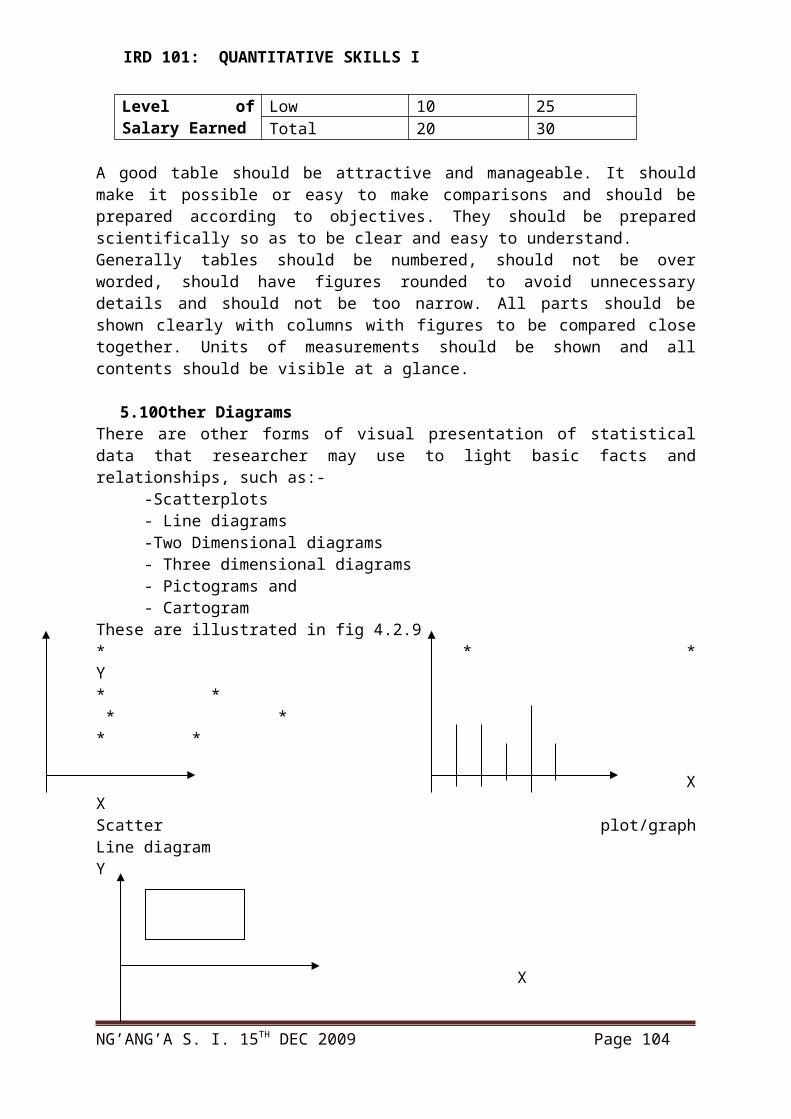
IRD 101: QUANTITATIVE SKILLS I
single sample, it is known as single sampling. When the decision is to be taken on the basis of two samples, it’s known as double sampling, and in the case where decision rests on the basis of more than two samples but the number of sample is certain and decided in advance, the sampling is known as multi-sampling. But when the number of sampling is more than two but is neither certain nor decided in advance, this type of system is often referred to as sequential sampling.
Non-probability (purposive sampling) The common feature of getting a non-probability sample is not based on the probability with which a unit can enter the sample, BUT, by other considerations such as common sense, experience, intuition, and expertise. They have limitations of being biased, unconscious errors of judgment, personal likes and dislikes, the attitude of the person sampling and so on. There is no objective way of assessing the magnitude of these errors.Non-probability or purposive sampling methods include;
i. Representative sampleSample selected in general, represents a characteristic variable and may not represent to other variables.
ii. Judgment sampleThe researcher after considering all the units of the population makes a judgment selection of some units to form his sample
iii. Accidental sampleResearcher selects any case he comes across. Method used to sample/survey quickly public opinion.
iv. Voluntary sampleRespondents volunteer to participate in a sample
v. Quota samplingKind of stratified judgment sampling. Samples of prefixed size are taken from each stratum using judgment sampling techniques. Each enumerator fills his quota in each stratum by taking advantage of any information that enables him it cover his quota quickly and cheaply.
NB. It is not possible to know whether the sample is representative or not.
Sample size determinationDetermined by: i) resources
ii) Requirements of the proposed plan of analysis.The sample size must be large enough to:-
i Allow for reliable analysis of cross- tabulationsiiProvide for desired level of accuracy in estimates of the larger population
iii.Test for significance of differences between estimators.
Minimum sample sizeM = 50 when M = minimum sample size Ps Ps = proportion of total cases expected in the smallest category of the
variable.According to Krejcie (1990), reported by Michael et el (1971) the sample size is determined by;
S = x 2 NP(1-P)
NG’ANG’A S. I. 15TH DEC 2009 Page 104

IRD 101: QUANTITATIVE SKILLS I
D2(N-1) +x2 P (1-P)Where
S =desired sample sizeN =populationP =population proportion (take 0.5)D =degree of accuracy reflected by the amount of error that can be tolerated in
fluctuation of a sample proportion (p) about the population. Take D = 0.05 equal to 1.96 6p at 95% confidence level.
6ᵨ = standard error of the proportion
.x = table chi square for one degree of freedom relative to the desired level of confidence. (x = 3.841 for 95% confidence level.)
Substituting the constants in the relationship above.
.s = 0.96025N 0.0025(N-1) + 0.96025
WhenN = 318, the sample size is;
.s = 0.96025N 0.0025(371) + 0.96025
= 305.3595 1.75275
= 174NB. A sample size of 174 represents a proportion of 54.72% of the population, which is too high and costly to survey.
According to Nassiuma (2000), the sample size can be determined by;
S = .N(cv2)
Cv2 + (N-1) e2
Where S = sample sizeN = population
Cv = coefficient of variation (take 0.5)
.e = tolerance of desired level of confidence (take 0.05) at 95% confidence level)
Substituting the constants;
S = 0.25N 0.25 + 0.7925 = 76
A sample size of 76 would represent a proportion of 23.9% of the population.
NG’ANG’A S. I. 15TH DEC 2009 Page 105
IRD 101: QUANTITATIVE SKILLS I
Useful table for determining the sample sizeBased on the above model by D. Morgan (1990), the following sample sizes are recommended for corresponding populations.
Population size
sample Population size
Sample size Population size
Sample size
10 10 100 80 4000 35120 19 150 108 5000 30730 28 200 132 10000 37040 35 250 162 20000 37750 44 300 169 50000 38160 52 400 196 10000 38470 59 1500 30680 66 2000 32290 73 3000 341
6.1.2 Sample Examination Questions -Sampling
1. a) A management Consulting firm based in Nakuru has been commissioned by BP Shell to evaluate the company’s Human Resources (HR) capacity needs in relation to its performance. The company has four major categories of staff as follows:
Finance and administration 300Information technology 100Marketing and production 450Research and development 150
1) Giving reasons, suggest a suitable sampling techniques for the above study (4 marks)
2) Develop a suitable sampling design comprising of x 200 staff (8 Marks)
b) Explain why sampling is preferred to complete enumeration. (8 marks)
2
a. Explain four criteria for a representative sample that is suitable for an effective survey research in Business management studies.
b. A researcher engaged in a Business Management research study for an organization is required to investigate consumer perceptions on product/services quality with a view
NG’ANG’A S. I. 15TH DEC 2009 Page 106
IRD 101: QUANTITATIVE SKILLS I
to establishing its impact on overall sales volumes in the company. The company has a variety of customers on the basis of income groups, age-groups among other characteristics. Soft Drink products and confectioneries constitute a major component of the company’s sales volumes. However, the target population of customers is wide, and no suitable sampling frame is available.
i) Suggest with reasons, a suitable sampling method for the study. (6 Marks).ii) Using the selected sampling method (i) above, explain how the researcher
could obtain a sample of approximately 1,000 customers. (10 marks).
3a) Differentiate between qualitative and quantitative research studies. (10 marks)b) Write brief notes on the following:
i. Stratified Sampling (2 marks)ii. Convenient Sampling (2 marks)
iii. Sampling frame (2 marks)iv. Systematic sampling (2 marks)
a) By giving example, explain why a researcher may resort to samplings and not conducting complete enumeration. (8 marks)Discuss at least three characteristics of a good sample (6 marks)Differentiate between probability sampling and non-probability sampling (4 marks)
4Distinguish between random and non-random sampling procedures. (8 marks)State the difference between the terms “sample” and “population” as used in Business Management ResearchFor the sample to be acceptable it must meet certain conditions. Which are these conditions?
5Abdul Onyango is a research worker with a reputable research consultancy firm that has won the right to conduct a market research study for a client. He wishes to collect data for the study from shopkeepers operating in the downtown shopping area of Nairobi. What would be the most suitable technique? (4 marks)Justify the choice of ht sampling technique. (10 marks)
Explain giving examples what is understood by: (i) Stratified sampling (4 marks)(ii) Judgment sampling (4 marks)
6A researcher undertook to study how social background influences academic achievement. He considered a population of 600 people. Whose composition was: 90 professionals. 115 managers. 150 skilled workers, 120 unskilled workers, and 125 businessmen.
What would be the most suitable sampling method for the study (4 marks)Justify the use of such a sampling method. (4 marks)Show how a sample of 240 would be drawn from the population. (10 marks)
NG’ANG’A S. I. 15TH DEC 2009 Page 107

IRD 101: QUANTITATIVE SKILLS I
Indicate the composition of each category of the population in the sample (2 marks)
7As the first step to data collection. It is important to seek information from secondary sources Explain in briefly the difference between primary and secondary data. (2 marks)What are the merits and demerits of secondary data over primary data? (8 marks)
Discuss the factor that influences sample size in research.
8Mary Mwangi is a K.I.M research student who wishes to collect primary data from a population in meta estate in Nairobi. These is divided into 5 (five) blocks of 60, 75, 80, and 45 housing units.What sampling procedure should Mary use? What?Show how she could choose a sample of 75 units.Can she use a sample random sampling? How?
10Explain by giving examples what is meant by:
a. Systematic random sampling.b. Convenience sampling c. Cluster random samplingd. Quota sampling
11Research data is a reputable research consultancy firm that has worn the right to conduct a study of the effectiveness of a newly developed teaching method at the Kenya institute of management (KIM). If research data were to use DBMS classes (i.e. group a-d) as there target population;What would be the most appropriate sampling technique to use? (4 marks)Justify the choice of (a) above (8 marks)In what way can simple random sampling be used? (8 marks)
NG’ANG’A S. I. 15TH DEC 2009 Page 108

IRD 101: QUANTITATIVE SKILLS I
6.2 Methods of Data collection
Instrumentation – research instrumentsInstrumentation is the process of selecting and developing measuring devices and methods appropriate to a given research problem. Research instruments are devices, which assist researchers in collecting necessary information or data.
Requirement of the research instrumentsMust be: i) valid – measure what it claims to measure. Relevant.( i.e. with respect to content as expressed by objectives).
ii) Reliable – stable, consistent, accurate, dependable and predictable.ValidityExtent to which a research instrument measures what it is designed to measure. Three types of validity; content validity, predictive validity and predictableContent validity
Two varieties – face validity and sampling validityFace validity is concerned with the extent to which the research instrument measures what it appears to measure according to the researcher’s subject assessment.Sampling validity refers to the extent to which the research instrument adequately samples the content population of the property being measured.
Construct validityConcerned with the extent to which a research instrument serves to predict some meaning, traits or constructs in the candidate; data contained from a research instrument should accurately reflect or represent a theoretical concept.
Predictive validityRefers to the degree of correlation between test scores and some future outcome, such as job success.Concurrent validity predicts behavior of subjects in the present.
Validation of the research instrumentProcess of collecting evidence to support the inference attached to the information obtained. The presence or absence of systematic error in data largely determines validity.Techniques of validating
i) Construct validitya. Variable being measured clearly definedb. Hypothesis based on a theory underlying the variable formed.c. The hypothesis tested – logically and empirically
Construct validity in a study can also be assessed if two or more different instruments are used to measure the same concept.Triangulation; methodological, source and or investigator
iii) Content validityContent validation is a matter of determining if the content that the instrument contains is adequate. It also checks the format of the instrument
Use expert opinion to the content and format of an instrument to judge whether or not it is appropriate.
iii) Criterion – related validityPredictive and concurrent validity – not common in research
NG’ANG’A S. I. 15TH DEC 2009 Page 109

IRD 101: QUANTITATIVE SKILLS I
Determining the reliability of the research instrument
Three methods: i Test retest methodA research instrument administered to the same group of persons. The score on the two sets of measures are then correlated to obtain an estimate computed –coefficient of reliability.iiParallel – forms technique (equivalent form method)The two sets of instruments administered to a group of persons. The score on the two sets of measures are then correlated to obtain estimate reliability –coefficient of reliability.
iii Internal consistency method
Single instruments administered. There are three types.a) Split - half method
The research instrument is separated into two sets of questions – even numbered and odd numbered questions. The two sets of items scored separately and then correlated to obtain an estimate of reliability. The reliability coefficient is calculated using the SPEARMAN – BROEN prophecy formula:-
Reliability of scores on the total tests – 2(reliability for half test) 1+ reliability for ½ tests
Suppose that a test has a known reality. The spearman – brown formula
rn = nr 1+ (n-1)r
Estimates the reliability of the score from a similar test n time as long with homogenous content
Where r = the original reliability Rn = reliability of the test n time as long N = can be a fraction (shortened) or a whole number (lengthened) test
b) Kuder – Richardson approaches
Method of rational equivalence. The Kuder-richardson formulas 20 and 21 provide relatively estimates of the coefficient of equivalence. Formula21, less accurate, but simple to compute.
rRKR21 = k 1-[ m(k-m)] k- 1 Ks2
Where : items are scored 1 point if right and 0 point if wrongM = meanK = number of itemS = standard deviation
c) alpha coefficient (crowbach – {α} = KR20 α = KR20 = K (S2 - ∑S
2)S2(K- 1) Where k = number of items used to measure
NG’ANG’A S. I. 15TH DEC 2009 Page 110

IRD 101: QUANTITATIVE SKILLS I
S2 = variance of all scores S2 = variance of individual items
KR20 = reliability coefficient of internal consistence.
NB. High co efficiency implies that items correlate highly among themselves, i.e. there is consistency implies that items correlate highly themselves, i.e. there is consistence among the items in measuring concepts of interest.
Types of research instruments Surveys are the most widely used technique in social science education and
the behavioral science for the collection of data. They are as means of gathering information that describes the nature and
extent of a specified set of data ranging from physical counts and frequencies to attributes and opinions.
Type survey includes: survey or records, mailed questionnaire, telephone survey, group interviews, individual interviews.
Characteristics of survey techniquesI. Guiding principals underlying surveys are that they should be
II. Systematic – carefully planed and executed to injure appropriate content coverage, sound and efficient data coverage.
III. Representative – closely reelecting the population of all possible cases or occurrences, either by including everyone or everything, or by using scientific sampling procedures.
IV. Objective – ensuring that the data are observable and explicit as possible.V. Quantified – yielding data that can be expressed in numerical terms.
Limitations of survey techniques
Survey methods, with exception of record survey, run the risk of generating misleading information due to:-
1. Survey only tabs respondents who are accessible and co-operative.2. Surveys make respondents feel special or unnatural and this produce responses that
are artificial and/or slanted.3. Surveys arouse ‘response sets’ such as acquiescence or a proneness to agree with
positive statement or questions.4. Surveys are vulnerable to over-rate or under-rates bias the tendency for some
respondents to give consistently high or low ratings.5. In case of interviews, biased reactions can be elicited because of characteristic of the
interviewer or respondents, or the combination that elicit an unduly favorable or unfavorable pattern or responses.
General Guidelines for Designing Surveys
1. Define the purpose and scope of the surveys in explicit terms
NG’ANG’A S. I. 15TH DEC 2009 Page 111
IRD 101: QUANTITATIVE SKILLS I
2. Avoid using an existing survey. If it was designed for a different purpose, population circumstances.
3. In designing questionnaires or interviews, one often finds its helpful to sit down with a group of potential respondents and explore what is meaningful or important to them, and how best to phrase questions to reflect their attitudes or opinions.
4. Field test instruments, to spot ambiguous or redundant items and to arrive at a format leading to ease of data tabulation and analysis.
5. Examine the merits of using machine-score answer sheets to facilitate tabulation and analysis.
6. As often as possible, use structured questions as opposed to unstructured and open-ended ones for uniformity or results and ease of analysis.
7. Do not ask questions out of idle curiosity. 8. Avoid loaded or biased questions be watchful or biased sampling.9. Keep the final product as brief, simple, clear and straightforward as possible. 10. Brainstorm the analysis needs to insure the clarity and comprehensiveness of
instrument.11. Consider the necessary and sufficient characteristics of the respondent that must
be collected at the time the survey is administered and on which the data analysis will be based.
12. Imagine various outcomes that might result from the survey, including surprising ones. This helps to anticipate gaps or shortcomings in the approach and may indicate the need for more background information about the respondents or additional questions.
The most common research instruments used social science survey technique includei Questionnairesii Interview schedulesiii Observational formsiv Standardized tests.v Records survey
The following is a summary of the types, characteristics advantages and limitations of the research instruments.
i Open-ended Questions- Receives the Answer open to what a responded wishes to give.
Advantages: Free expressions, responses not biased and used to start a depth interview, sets interview at ease.Limitation: No specific answers: may digress; compiling, tabulating and interpreting the responses could be difficult.
ii Dichotomous Questions - Receives only two types of responses – Yes/No; True/False; one or two choices; can be varied to have a third or fourth opinion – not decided; Do not know e.t.c- The responses can be scored by percentage.
Limitation: Opinion questions require a variation of approval or disapproval.
iii Multiple choice Questions - A choice of responses offered. Respond by ticking/circling and/or fill in blank.
NG’ANG’A S. I. 15TH DEC 2009 Page 112
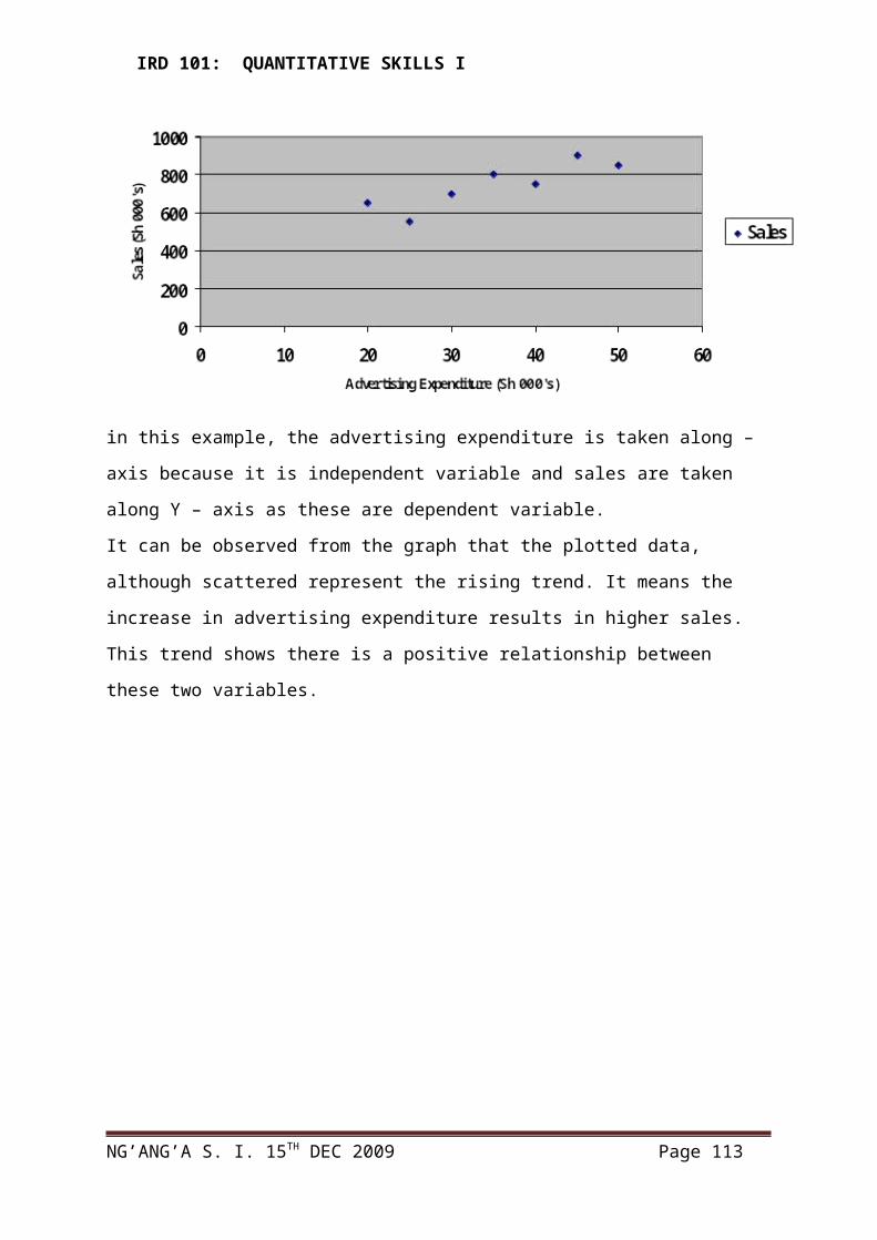
IRD 101: QUANTITATIVE SKILLS I
iv Declarative Question- Respondents give reactions to a given series of statements-Good,
Satisfactory, Fair or Poor.Types of Questions to Avoid
1) Misleading questions2) Leading questions 3) Double barreled questions4) Embarrassing question5) Ambiguous/argue questions.6) Uninformative questions.
CHARACTERISTICS OF RESEARCH INSTRUMENTS
RESEARCH INSTRUMENT
CHARACTERISTICS ADVANTAGES LIMITATIONS
1. QUESTIONNAIRE1) Open ended
questions2) Closed and
pictorial- Multiple choice- True/false- Structured – fill in blanks
A set of carefully selected an ordered questions used in sampled studies.- Indicate topic of study - Should be attractive,
neatly, arranged, clearly printed/typed
- Objective, simple and clear question.
- - In a local or understandable language.- Should be accompanied by a letter of transmittal.
- Are inexpensive- Wide ranging- Can be well
designed, simple and clear.
- Self – administering- Can be made
anonymous.
- Low response rate can occur.
- No assurance the questions were understood.
- Language may not be to level of respondent
- Suspicious respondents deliberately give false information.
- May leave out important information required by study.
2. INTERVIEW SCHEDULES
1) Telephone interviews
2) Group interviews.
3) Individual interviews.
May be - Unstruc
tured - Semi
structured.
- Structur
- An interview is a formal meeting or communication framework between two parties whose primary objective is the procurement of factual information
- Plan what will be done during the interview.
- Kind of questionnaire may be used to help collect data required in a standardized way.
- List desired questions in a given order.
- Allow face to face contact between the researcher and respondent
- Respondent can seek clarification of a question not clear.
- Researcher can evaluate sincerity and insight of the responded.
- Allow researcher explain purpose of research
- Researcher may stimulate
- Unstructured interview often yield data which is difficult to summarize or evaluate.
- Can be costly in terms of money and time.
- Bias may creep in personal class
- Vulnerable to personality conflicts.
- Requires studied and
NG’ANG’A S. I. 15TH DEC 2009 Page 113
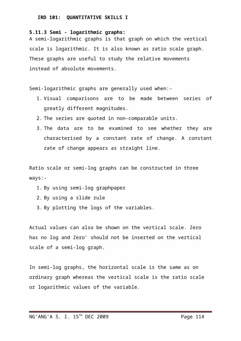
IRD 101: QUANTITATIVE SKILLS I
ed - Record the interview – note taking, tape recording.
respondent to a greater extent
- Appropriate language and intellectual difficulties exists.
trained interviewers.
3
OBSERVATIONAL FORMS
i. Systematicii. Participant/
ecological iii. Archival
records iv. Simulations.v. Ethnography
vi. Case studiesvii. Content
analysis.
Systematic ObservationRecording and encoding a set of natural behavior usually in their natural setting for the purpose of uncovering meaningful relations
Steps- Choose natural
behavior to observe.- Select appropriate
observational setting.- Decides on the mode of
recording observations.- Determine sampling
strategies.- Train observers and
observe.- Analyze data-structured
or unstructured.
Participant observation - Used in field studies- Non-experimental- Researcher is there and
involved (naturalistic) not very active by passive.
Archival observation - Statistical records that
allow the researcher to observe the effect and courses of real word events
- National records – statistical records, written documents, mass communication.
- Observation better than self reports obtained from questionnaires and interviews.
- Natural setting is used.
- Activities that could not be investigated easily like mob justice, natural disasters are recorded and easily access.
- Yields more qualitative information
- Enable researcher to obtain detailed information.
- Ecological observation can be reflected hence verifiable.
- Ecological observation can be reflected hence verifiable.
- Economical in terms of time and money.
- Data real because it is collected under natural condition
- Gathering of information does not require the cooperation of the individual/subject.
- Suitable for large-scale study of
- Hawthorne effect – effect of the observer on the observed.
- Observed may question.
- Halo effect on the observer may lead to confusion.
- Sense organs may be inadequate to observe.
- Costly in time and money.
- Some complex behavior of the subject may be difficult to observe.
- Information obtained lacks verification (cannot be verified).
- Lacks statistical analysis.
- Lacks rules which can be understood in order to collect, analyze qualitative information.
- Can lean to a lot of bias
- Can be risky.
NG’ANG’A S. I. 15TH DEC 2009 Page 114
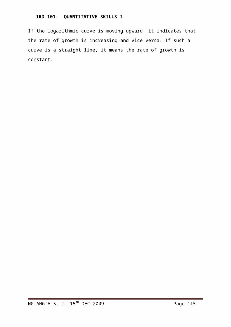
IRD 101: QUANTITATIVE SKILLS I
phenomena.4 RECORD SURVEY - Differ from those in
other survey types because they are non-reactive i.e they do not involve a responsive from people.
- Records are non-reactive
- They are inexpensive
- Allow historical comparison and trend analysis.
- Are accurate and up to date they provide an excellent baseline for comparison
- May involve confidential restrictions.
- Are often incomplete, inaccurate, out of date or unavailable.
- Changing rules for keeping records often makes year to year comparison invalid.
- Can be misleading unless knowledgeable person can explain how the records were complied.
- Purpose of records is often unrelated to purpose of survey.
- Factual data (no input on values or attitudes) are present.
5 STANDARDIZED TEST & SCALES
ii. Intelligence & Aptitude tests Achievement tests
iii. Attitude scales. - value scales- Lickert type or
summated rating scales.
- Thurston type or equal appearing interval scale
- Gutiman type or cumulative scale.
- Tests are systematic procedure in which individuals are presented with a set of constructed stimulus to which they respond, the responses enabling the tester to assign the taste a numeral or set of numerals from which inferences can be made about the taste’s possession of whatever the scale is supposed to measure
- Not common in social science research
- Mainly used in education
Not common standardized tests/scales available for social sciences research.
6.3 DATA ANALYISIS
NG’ANG’A S. I. 15TH DEC 2009 Page 115

IRD 101: QUANTITATIVE SKILLS I
6.3.1Introduction
One of the biggest challenges in research is designing a study with known and specified variables whose measures are obtained in data collection, using an appropriate research instrument. The data collected should be analyzed either qualitatively or quantitatively. This section looks at how data is analyzed and presented. It will enable a researcher choose a data analysis method to be employed in his/her study and thus design the study instrument to collect the data as required.
6.3.2 Qualitative data analysis
Qualitative research investigates the quality of relationships, activities, situations and materials where attributes and characteristics of interest are studied. Attributes are any qualities ascribed to a person, subject or symbol and are essentially deemed to be a permanent quality of a thing. Characteristics are distinguishing traits or features of the object under study. In qualitative research, greater emphasis is placed on holistic description. This is describing in details what goes on in a particular activity or situation rather on comparing the effects of a particular treatment.
Qualitative research attempts to determine how people make sense of their lives in a natural setting and the research is the key instrument. Data is collected in form of words or pictures rather than numbers and concern is on both the process as well as the final results. Data is analyzed through description and induction as outlined in the procedural steps below:
Step 1: Organization of dataOrganize data to indicate how the data will be classified and tabulated according to research questions and objectives and how the information will be analyzed, and synthesized and presented in reports.
Step 2: Editing of dataEdit data to ensure accuracy and uniformity in report and to acquire maximum information from the data. Check for inconsistencies; mistakes; lack of uniformity; illegibility and blank or missing responses that should be disregarded. Check also for out layers that are likely to distort the general picture portrayed by the sampled respondents and expected of the population.
Step 3: Summarize dataPrepare summaries of data in questionnaires, interviews schedules and observation guides by:a) Tabulating the number of responses received from the instrument for each itemb) Prepare a summary or a master questionnaire into which you put totals of responses onto a blank instrument.c) If endowed with or can access computer data analysis software such as the Statistical Package for Social Scientists (SPSS), enter the data.
This makes analysis easier, presents concise summary statement of statistical findings, facilitates comparisons, assists in interpretation of finding and provides a brief statement of purpose, methods and data of a study.
Step 4: Interpretation of Responses
NG’ANG’A S. I. 15TH DEC 2009 Page 116
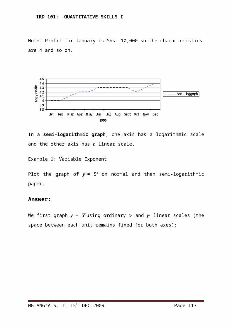
IRD 101: QUANTITATIVE SKILLS I
Research questions are related to research problem, objectives and/or hypothesis and responses may be interpreted with assistance of any of the following techniques.
More or less index:This is computed to show the proportion of respondents whose choice is more or less favorable. Thus: Index = “more” – “less” Total responsesThe person answering the same or undecided is not included in the index. This index has a shortcoming in that no measure is provided for the type of change required or expected.
Rating scale:This scale rates the opinion of the respondents on a continuum such as the lickert scale. An example is the 5 point scale where the frequency and percentage of respondents selecting a particular response is computed indicating the general perception of the sampled respondents.
5 4 3 2 1Strongly agree agree neutral disagree strongly disagree
OR
5 4 3 2 1Very favorable favorable neutral unfavorable very unfavorable
It is also possible to obtain and test the overall position taken by all the respondents put together by computing the mean score on each item and using a one sample t-test using a test statistic of the highest rating plus the lowest rating divided by 2, to check the significance of the difference between the mean and the test statistic. For example, in the 5 point lickert scale above, the test statistic is 3. If the mean score in any item is higher than 3 numerically and the test shows that the difference is significantly higher than 3, then all respondents put together lean more towards agree and it is interpreted to mean that the respondents in general, are in favor of the statement or construct in the question.
Interpretation weightingAs in the rating scale, respondents rate a statement/position on a variable. The ratings are assigned to correspond to a score or weight. The weight and number of respondents, frequency in favor of a certain position are then multiplied to give an interpretation weighting. If on the five point lickert scale labeled 5, 4, 3, 2, and 1 are taken as weights, then tabulating the results yields:
Scale weight No of responses weight x no. of responses (W) (F)Strongly agree 5 30 150Agree 4 25 100Undecided 3 20 60Disagree 2 15 30Strongly disagree 1 10 10 ∑W ∑F 100 350
Average weight (mean) = ∑W *hF = 350 = 3.5
NG’ANG’A S. I. 15TH DEC 2009 Page 117
IRD 101: QUANTITATIVE SKILLS I
∑F 100
The average weight 3.5 lies higher than 3, the midpoint of the lickert scale and it is interpreted that the respondents agree with the proposition.
Indexes of fame or popularityThis is an index that can be used to rate the popularity or notoriety of an individual. To develop this index, questions are asked that lead to a list of names of who ascribe to a given concern. The list of names and the number of times the name is mentioned is then used to calculate the index as shown table 5.1.
Table 5.1: Computation of an index of fame
Names No. of times the name mentioned
FIndex of fame= F ∑F
A 60 0.30B 40 0.20C 50 0.25D 20 0.10E 30 0.15
TOTAL 200
This is a continuum ranging from 0 to 1. The closer a name is to 1, the more popular or notorious the person is according to the respondents depending on the measure of interest.
Cross TabulationThis is done to obtain and present more information that can be obtained in a single classification. It contains a matrix of classes of values and may contain one or two variables, original figures or percentages or both. It improves understanding of the data, cross effect of the variables and forms a basis for comparison. An example can be seen in the composition of residents in a residential area in Nairobi.
Table 5.2: Cross-tabulation of residents in a residential area in Nairobi in 1980 according to race and gender
ETHICITY POPULATION IN AN AREA/TOWNMALE FEMALE TOTAL
AsiansEuropeanAfricans
3,00060015,000
5,00080016,000
8,0001400031,000
TOTAL 18,600 21,800 40,400
While cross tabulations are used to interpret data of various variables, they also form a basis for comparisons; they can be used further for quantitative analysis in testing of relationships between variables using chi-square. For example, if data leads to a cross tabulation of data on the basis of two variables, visits by quality standards and assurance officers to secondary schools, and classification of schools according to performance in English, it can be used to
NG’ANG’A S. I. 15TH DEC 2009 Page 118

IRD 101: QUANTITATIVE SKILLS I
test whether there is an association between the number of visits and the performance in English at the KCSE level as shown in table 5.3.
Table 5.3: Cross-tabulation of quality assurance and standards officers visits to schools and the classification of schools in English according to performance at the KCSE level
Classification of schools according to performance in English at the KCSE level
QASO number of visits to schools
High Average Low TotalVisitedNot visitedTotal
Frequency distributionRatios and proportions in percentage of respondents in favor of a given response among mutually exclusive responses are also used in the interpretation of data. The proportion of respondents in favor of a certain response is calculated and tabulated as shown in table 5.4. If a sample of registered voters were asked whether they would vote in favor of a certain candidate the responses would be yes, no or no response. Table 5.4: Frequency distribution of respondents in favor of a certain candidate in an election
Response frequency ProportionYesNo Missing
80700
53.346.70
Total 150 100
This would be interpreted to mean that the candidate is likely to win in the election although s/he has a significant proportion (46.7%) of the respondents who are opposed to his/her candidature.
If the researcher wishes to find out more about the electorate, the frequency distribution could be broken down to show the distribution according to gender, age, level of education, occupation of the respondents so that the candidate could be advised on the strategies to adopt targeting specific stratum of respondents. The frequency distribution according to gender is shown in table 5.5.
Table 5.5: Frequency distribution of respondents in favor of a candidate in an election according to gender
RESPONSE MALE FEMALE TOTALF % F % F %
YesNo Missing
30400
2026.70
50300
33.3200
50700
55.347.30
Total 70 46.7 80 53.3 100 100
This may be interpreted to mean that more women (33.3%) as compared to men (20%) are in support of the candidate.
NG’ANG’A S. I. 15TH DEC 2009 Page 119

IRD 101: QUANTITATIVE SKILLS I
This data analysis can be done manually by use of tallies against individual responses and a hand calculator to compute proportions. For example, if only 40 respondents were sampled in the example above, then Total respondents proportion (%) Yes 28/40 = 70 % No 12 = 30% 40 This can then be entered into the frequency distribution table.
A computer package (software) such as SPSS can also be used to analyze qualitative data obtained from respondents in social science. Questions in the research instruments are coded, variables defined and entered into the computer after responses are entered as either numeric or string from which frequency distributions can be generated.
6.3.3 Quantitative data analysisQuantitative research refers to the studies that make use of a numeric measure to evaluate an aspect of a particular problem or situation. Such studies are done when a researcher wishes to obtain a large body of data to perform statistical analysis and produce results that can be generalized to the target population. Data is reduced to numeric scores and preference is given for a random technique of obtaining meaningful samples.
In quantitative studies, data is statistically analyzed so that meaning is inferred. Quantitative research is mainly concerned with the problem of estimation and testing statistically based hypothesis. This is achieved through descriptive statistics from which population parameters are estimated leading to generalizations. Quantitative research assumes that behavior of people can be objectively measured and the cause and effect relationship between variables determined through various techniques. The following sections explain how numeric data obtained from quantitative research is analyzed.
The following is a general step by step procedure followed in quantitative research:i) Collect quantitative dataii) Obtain descriptive statistics iii) Estimate population parameter from the statisticsiv) Test hypothesisv) Make inferences
6.3.4 Descriptive statisticsDescriptive statistics provide information on how data obtained in respect to variables of interest relate to each other. There are four categories under which data can be analyzed to provide descriptive statistics: measures of central tendency, measures of dispersion, measures of skewedness and measures of peakedness.
6.4Measures of central tendency These measures show how quantitative data obtained from respondents or from the study tends to coalesce, or cluster towards a certain center. The most common measures of central tendency used in research are the mean, the median and the mode.
NG’ANG’A S. I. 15TH DEC 2009 Page 120
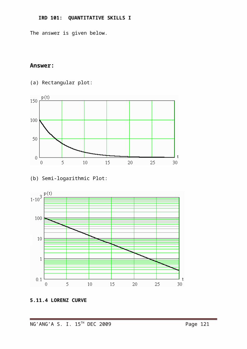
IRD 101: QUANTITATIVE SKILLS I
i) The mean
The arithmetic mean is the measure of central tendency normally thought of as an average. It is given by: n
Sample mean for ungrouped data
for grouped data
for grouped continuous data Where: ∑ = sum or summation of f = frequency (number of time the same response is obtained) x = observation n = sample size = mean m = is the midpoint of class obtained by adding the lower class limit and upper class limit and dividing by two.
ii) The median
This is the middle observation after data have been put in an ascending ordered array. If the number of observations (n) is odd, the median is the middle one e.g. in 32, 41, 59, 63, and 71; 59 is the median. If n is even, the median is the middle 2 divided by 2
e.g. in 41, 59, 63, and 71, the median is
For grouped data:
When Lmd = lower class boundary of the median class. f = cumulative frequency of the class preceding the median class. fmd = the frequency of the median class. c = class interval of the median class.
iii) The modeThe mode is the observation which occurs most often. In grouped data, the class with the largest frequency is the modal class.
NG’ANG’A S. I. 15TH DEC 2009 Page 121

IRD 101: QUANTITATIVE SKILLS I
Where Lmd = the lower class boundary of the modal class. Da = the difference between the frequency of the modal class and the class
preceding it. Db = the difference between the frequency of the modal and the class after it. c = the class interval of the modal class.
Examples 5.1Kamau Otieno consultants conducted a study on the unemployment pattern in Nairobi which produced the following results:
Age (years) number unemployed (000’s) Men Women
15-19 15 1020-24 19 1325-29 28 2230-34 30 2535-39 23 2140-44 18 945-49 17 00 150 100
Mean age of unemployed respondents
MALE FEMALEClass age frequency midpoint fm f fm(years) f m 15-19 15 17 225 10 17020-24 19 22 418 13 28625-29 28 27 756 22 59430-34 30 32 960 25 80035-39 23 37 851 21 77740-44 18 42 756 9 37845-49 17 47 752 0 0 ∑f = 150 ∑fm = 4748 ∑f= 100 ∑fm = 3005
Mean age of unemployed men
NG’ANG’A S. I. 15TH DEC 2009 Page 122

IRD 101: QUANTITATIVE SKILLS I
Mean age of unemployed women
The mean age of all respondents together
The median age of the unemployed
MALE FEMALEClass (age) f Cf f cf15-19 20-24 25-29 30-34 35-39 40-44 45-49
15192830231817
15346292115133150
101322252190
1023457091100100
The middle age of the unemployed men is the 75th which is in the class 30-34 as shown in the cumulative frequency distribution.
Median age h
Lmd = 30 f = 62 (cumulative frequency of the classes before the class containing the
median item). fmd = 30 n = 150 c = 5
Median age of unemployed men
Median age of unemployed women
The mode of the age of the unemployed respondents
NG’ANG’A S. I. 15TH DEC 2009 Page 123

IRD 101: QUANTITATIVE SKILLS I
From the cumulative frequency distribution above, the modal class is 30-34
FOR MALE FOR FEMALE
Mode age of unemployed men
Mode of unemployed women h
Deductions On the whole: (i) The data suggests that there are more unemployed men than women in
Nairobi but the difference between the means of the two independent samples Male and Female is small and should be
subjected to significance testing by use of t tests. (ii) The unemployed are in their early thirties
6.5 Measures of DispersionThese measures show how data tends to scatter, spread, disperse or vary. They show variations or variability and as noted earlier there are three causes of variability in research data. These are variations caused by systematic or natural causes also said to be attributable causes, extraneous variables that require efforts to control or eliminate in a study or errors either in measurements or in use of instruments. Efforts are made to control extraneous variables by the research design and minimize variation due to errors by use of appropriate methods; instruments and random sampling while systematic variations are the objects of the study.
Dispersion or extent of spread is measured through computation of the range, quartile deviation and percentiles, mean deviations, variance, standard deviation and coefficient of variation.
i) The Range The range is the difference between the highest observation and the lowest observation. In frequency distribution, the range is taken to be the difference between the lower limit of the class at the lower extreme of the distribution and the upper limit of the class at the upper extreme. In example 5.1, the range is 49-15=34.
ii) Quartile DeviationsA quartile divides an array of data into four equal parts. Q1 gives the value of the item at the 1st quarter mark while Q3 gives the value of the item at the 3rd quarter mark. The semi-quartile range or quartile range deviation (QD) is given by:
NG’ANG’A S. I. 15TH DEC 2009 Page 124

IRD 101: QUANTITATIVE SKILLS I
which means 50% of the distribution lie
with the interval defined plus or minus the Quartile deviation.
iii) PercentileThese are values of a variable, which divide a set of ordered observation into 100 equal parts.
The 25th percentile is also called lower quartile.The 50th percentile is also called medianThe 75th percentile is also called the upper quartile.
The coefficient of
To calculate Q1 and Q3 in grouped continuous data
And
Where L1 and L3 is the lower class limit of the class with the ¼ th item and the ¾ th item respectively.
Lcf = lower cumulative frequency fq
th = frequency of the class that contains the ¼ or ¾ item.
The quartile deviation gives an indication about the uniformity or otherwise of the size of items of a distribution. Q.D. is a distance on a scale and thus regarded as a measure of partition.
iv) Mean deviationThis is the mean of the absolute values of the deviation from a measure of central tendency, usually the mean.
Mean absolute deviation (MAD)
OR MAD for grouped data
NG’ANG’A S. I. 15TH DEC 2009 Page 125
IRD 101: QUANTITATIVE SKILLS I
for grouped continuous data
(If mean is the measure of central tendency used )
The mean deviation is easier to understand and is affected by extreme values and is a better measure of dispersion compared to the range and quartile deviations. However, it is not suitable for further mathematical processing. v. The varianceThe variance is the mean of the squared deviation from their mean denoted by S2.
Sample variance
OR for grouped data
OR for grouped continuous data
vi The standard deviation
The standard deviation denoted by (s) is the square root of the variance
Sample standard deviation
for grouped data
And for grouped continuous data
The standard deviation is a good measure of dispersion since it takes into account all the data and responds to the exact position of every score about the mean. It is also sensitive to extreme score.
NG’ANG’A S. I. 15TH DEC 2009 Page 126

IRD 101: QUANTITATIVE SKILLS I
vi) Coefficient of variationThis is a measure of variability relative to the mean denoted by CV.
It is useful when comparing the spread of two distributions.
Example 5.2In the worked example 5.1 above, determine the group (male or female) which has greater variability (related dispersion) in unemployment.
Solution range ≥ upper class limit (upper extreme class) - lower limit (lower extreme class)
Suggest male have greater variability.
i) Quartile deviation
150
100
112.5
Unemployed male respondents have a greater variability in age based on quartile deviations.
NG’ANG’A S. I. 15TH DEC 2009 Page 127

IRD 101: QUANTITATIVE SKILLS I
ii) Coefficient of QD
iii) Mean absolute deviation (MAD)
From the worked example 5.1 was found to be 31.6 years for male and 30.05 years for male and 30.05 years for female.
MALE FEMALEclass f m │m- │ (m- )2 F(m- )2 f m- (m- )2 F(m- )2
15-1920-2425-2930-3435-3940-4445-49
15192830231817
17222732374247
-14.65-9.65-4.65=0.355.3510.3515.35
214.6293.1221.620.1228.62107.12235.62
3219.341769.33608.433.68658.321928.214005.58
101322252190
13.058.053.051.956.9511.9516.95
170.30640809.303.8048.30142.80287.30
1703842.43204.6695.061014.351285.220
∑f = 150
∑│m- │ =60.35
12192.89 │m- │= 41.95
∑f(m- )2= 5144.72
Mean deviation absolute deviation
From the calculation it can be noted that the interpretations have changed. The unemployed female respondents are shown here to have greater variability. This also suggests the female have higher deviation.
Coefficient of
NG’ANG’A S. I. 15TH DEC 2009 Page 128

IRD 101: QUANTITATIVE SKILLS I
iv) The variance
This measure suggests that male have greater variability.
V) The standards deviation
for grouped data
= √variance
For male For female This suggests that the male have greater variability.
Coefficient of variation (cv)
The coefficient of variation (cv) also suggest that the male have greater variability.
Table measure of dispersion for unemployed in Nairobi MALE FEMALE
RangeQuartile deviation (QD)Coefficient of QDMean absolute deviation (MAD)Coefficient of (MD)Variance (S2)Standard deviation (S)Coefficient variation
3413.9423%0.411.3081.839.0528.6%
294.8718%0.632.1%51.977.2124.0%
NG’ANG’A S. I. 15TH DEC 2009 Page 129

IRD 101: QUANTITATIVE SKILLS I
The measure shows that the unemployed males have high relative variability in age compared to female.
6.6 Skewness and Peakedness
6.6.1 Skewness
A distribution is said to be skewed if it is not symmetric. Skew distributions that often arise in practice are unimodal with one tail (upper or lower) longer compared with other tail. For those distributions the mean tends to lie on the same side of the mode as in figure 3.5
Fig: 5.5 skew distribution
mode median mean mean median mode
Fig 3.5 (a) is a positively skewed distribution with the lower (right) tail longer. The mean of the date is larger than median.Fig 3.5 (b) is a negatively skewed distribution with the lower (left) tail longer. The mean of the date is smaller than the median.In a normal distribution (one that is not skewed, all the three; the mean, mode and median coincide at the same point as shown in fig 3.5(c))
Fig 3.5(c) Mean,Mode,Median.
NG’ANG’A S. I. 15TH DEC 2009 Page 130

IRD 101: QUANTITATIVE SKILLS I
There are several ways of assessing skewness in a distribution: they include.i)
where µ is the population mean is the population size is the population standard deviation.
For a sample, coefficient of skweness (b1)
ii) Pearson’s coefficient of skewness (b1)
iii) Pearson’s absolute skewness = mean – mode OR
iv) Bowleys coefficient of skewness ( )
v) Bowleys absolute skewness
vi) Kelly’s coefficient of skewness (b1)
NG’ANG’A S. I. 15TH DEC 2009 Page 131

IRD 101: QUANTITATIVE SKILLS I
Where P50,P90 and P10 are the 50th, 90th and
10th percentiles.
Note:- The coefficient of skewness are relative measures and have no dimension while absolute measure have dimensions which are the unit for which x is measured.b- The direction of skewness is given by the algebraic sign (+ or-) and the numeric value gives the degree of skewness.c- The relative coefficient of skewness usually lies between +1 and -1. When b1 > 0, the distribution has a longer upper (right) tail and is very skewed. When b1 < 0, the distribution has longer lower (left) tail and is negatively skewed. When b1 = 0 the distribution is normal and is symmetric about the mean.
6.6.2 Peakedness (kurtosis)
Frequency distribution also vary in regards to their Peakedness is the extent to which a frequency distribution has a peak or is flat at the top.
Fig.4.6
Curve A is lepto kurtic
B is meso kurtic C is platty kurtic
Kurtosis is measured by B2 where
Note:A – in a normal distribution, B2 will be equal to 3.B – if B2 is greater than 3, the curve is more peaked (lepto kurtic).C - if B2 is less than 3, the curve is flatter at the top than the normal curve and is said to be (platy kurtic). A peak of a normal distribution is mesokurtic.
NG’ANG’A S. I. 15TH DEC 2009 Page 132

IRD 101: QUANTITATIVE SKILLS I
In research data analysis, coding and data entry is done in such a way that it allows generating of descriptive statistics by use of SPSS or excel.
6.7 Bivariate Data
Measures of central tendency, variability, and spread summarize a single variable by providing important information about its distribution. Often, more than one variable is collected on each individual. For example, in large health studies of populations it is common to obtain variables such as age, sex, height, weight, blood pressure, and total cholesterol on each individual. Economic studies may be interested in, among other things, personal income and years of education. As a third example, most university admissions committees ask for an applicant's high school grade point average and standardized admission test scores (e.g., SAT). In this chapter we consider bivariate data, which for now consists of two quantitative variables for each individual. Our first interest is in summarizing such data in a way that is analogous to summarizing univariate (single variable) data.
By way of illustration, let's consider something with which we are all familiar: age. It helps to discuss something familiar since knowing the subject matter goes a long way in making judgments about statistical results. Let's begin by asking if people tend to marry other people of about the same age. Our experience tells us "yes," but how good is the correspondence? One way to address the question is to look at pairs of ages for a sample of married couples. Table 1 below shows the ages of 10 married couples. Going across the columns we see that, yes, husbands and wives tend to be of about the same age, with men having a tendency to be slightly older than their wives. This is no big surprise, but at least the data bear out our experiences, which is not always the case.
Husband 36 72 37 36 51 50 47 50 37 41Wife 35 67 33 35 50 46 47 42 36 41Table 1: Sample of spousal ages of 10 White American Couples.
The pairs of ages in Table 1 are from a dataset consisting of 282 pairs of spousal ages, too many to make sense of from a table. What we need is a way to summarize the 282 pairs of ages. We know that each variable can be summarized by a histogram (see Figure 1) and by a mean and standard deviation (See Table 2).
Figure 1: Histograms of spousal ages. Mean Standard DeviationHusband 49 11Wife 47 11Table 2: Means and standard deviations of
NG’ANG’A S. I. 15TH DEC 2009 Page 133

IRD 101: QUANTITATIVE SKILLS I
spousal ages.
Each distribution is fairly skewed with a long right tail. From Table 1 we see that not all husbands are older than their wives and it is important to see that this fact is lost when we separate the variables. That is, even though we provide summary statistics on each variable, the pairing within couple is lost by separating the variables. We cannot say, for example, based on the means alone what percentage of couples have younger husbands than wives. We have to count across pairs to find this out. Only by maintaining the pairing can meaningful answers be found about couples per se. Another example of information not available from the separate descriptions of husbands and wives' ages is the mean age of husbands with wives of a certain age. For instance, what is the average age of husbands with 45-year-old wives? Finally, we do not know the relationship between the husband's age and the wife's age.
We can learn much more by displaying the bivariate data in a graphical form that maintains the pairing. Figure 2 shows a scatter plot of the paired ages. The x-axis represents the age of the husband and the y-axis the age of the wife.
Figure 2: Scatterplot showing wife age as a function of husband age.
There are two important characteristics of the data revealed by Figure 2. First, it is clear that there is a strong relationship between the husband's age and the wife's age: the older the husband, the older the wife. When one variable (y) increases with the second variable (v), we say that x and y have a positive association. Conversely, when y decreases as x increases, we say that they have a negative association.
Second, the points cluster along a straight line. When this occurs, the relationship is called a linear relationship.
Figure 3 shows a scatterplot of Arm Strength and Grip Strength from 149 individuals working in physically demanding jobs including electricians, construction and maintenance
NG’ANG’A S. I. 15TH DEC 2009 Page 134

IRD 101: QUANTITATIVE SKILLS I
workers, and auto mechanics. Not surprisingly, the stronger someone's grip, the stronger their arm tends to be. There is therefore a positive association between these variables. Although the points cluster along a line, they are not clustered quite as closely as they are for the scatter plot of spousal age.
Figure 3: Scatter plot of Grip Strength and Arm Strength.
Not all scatter plots show linear relationships. Figure 4 shows the results of an experiment conducted by Galileo on projectile motion. In the experiment, Galileo rolled balls down incline and measured how far they traveled as a function of the release height. It is clear from Figure 4 that the relationship between "Release Height" and "Distance Traveled" is not described well by a straight line: If you drew a line connecting the lowest point and the highest point, all of the remaining points would be above the line. The data are better fit by a parabola.
NG’ANG’A S. I. 15TH DEC 2009 Page 135

IRD 101: QUANTITATIVE SKILLS I
Figure 4: Galileo's data showing a non-linear relationship.
Scatter plots that show linear relationships between variables can differ in several ways including the slope of the line about which they cluster and how tightly the points cluster about the line. A statistical measure of the strength of the relationship between variables that takes these factors into account is the subject of the next section.
Quantitative Variables: Variables that have are measured on a numeric or quantitative scale. Ordinal, interval and ratio scales are quantitative. A country's population, a person's shoe size, or a car's speed are all quantitative variables. Variables that are not quantitative are known as qualitative variables.
Histogram: A histogram is a graphical representation of a distribution. It partitions the variable on the x-axis into various contiguous class intervals of (usually) equal widths. The heights of the bars represent the class frequencies.
Figure 5See also: Sturgis's Rule
Sturgis's Rule:
NG’ANG’A S. I. 15TH DEC 2009 Page 136
IRD 101: QUANTITATIVE SKILLS I
One method of determining the number of classes for a histogram, Sturgis's Rule is to take 1+log2N classes, rounded to the nearest integer.
Bivariate: Bivariate data is data for which there are two variables for each observation. As an example, the following bivariate data show the ages of husbands and wives of 10 married couples.
Husband36723736515047503741Wife 35673335504647423641Table 3
Scatter Plot: A scatter plot of two variables shows the values of one variable on the Y axis and the values of the other variable on the X axis. Scatter plots are well suited for revealing the relationship between two variables. The scatter plot shown in Figure 4 illustrates data from one of Galileo's classic experiments in which he observed the distance traveled balls traveled after being dropped on a incline as a function of their release height.
Positive Association: There is a positive association between variables X and Y if smaller values of X are associated with smaller values of Y and larger values of X are assoicated with larger values of Y.
Negative Association: There is a negative association between variables X and Y if smaller values of X are associated with larger values of Y and larger values of X are assoicated with smaller values of Y.
Linear Relationship: If the relationship between two variables is a perfect linear relationship, then a scatterplot of the points will fall on a straight line as shown in Figure 6.
Figure 6With real data, there is almost never a perfect linear relationship between two variables. The more the points tend to fall along a straight line the stronger the linear relationship. Figure 2 shows two variables (husband's age and wife's age) that have a strong but not a perfect linear relationship.
A dataset with two variables contains what is called bivariate data. This chapter discusses ways to describe the relationship between two variables. For example, you may wish to describe the relationship between the heights and weights of people to determine the extent to which taller people weigh more.
NG’ANG’A S. I. 15TH DEC 2009 Page 137
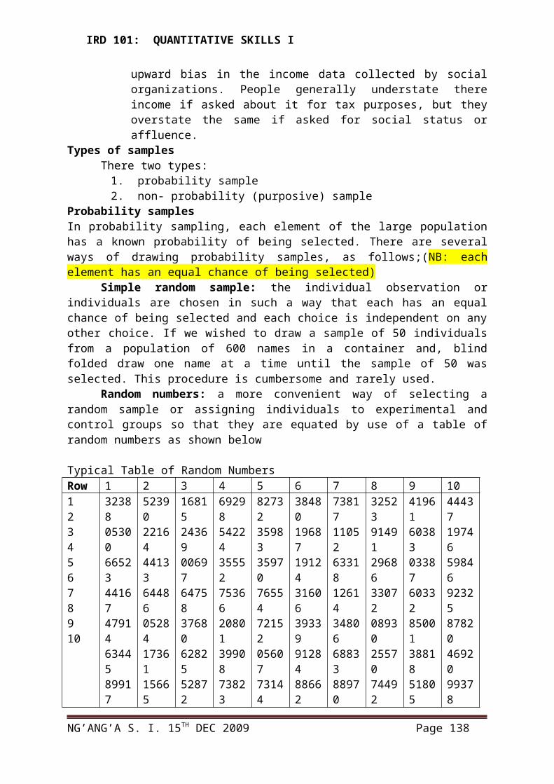
IRD 101: QUANTITATIVE SKILLS I
The introductory section gives more examples of bivariate relationships and presents the most common way of portraying these relationships graphically. The next five sections discuss Pearson's correlation, the most common index of the relationship between two variables. The final section, "Variance Sum Law II" makes use of Pearson's correlation to generalize this law to bivariate data.
6.8 Revision Questions
1. The following figures show the volume of commodity sales by three sales representatives (A-C) at Manga-Craft Ltd. in a period of 5 days.A 410 415 420 425 405 430 420 425B 415 418 417 416 415 414 413 412C 430 415 450 400 420 440 430 425
Calculate: a) The mean deviation for each set of sales (5 marks) b) The standard deviation for each set of sales (5 marks) c) What is the purpose of standard deviation? (5 marks) d) Comment on the standard deviation calculated in relation to the sales. (5 marks)
2. The following sets of data refer to a sample of marks (out of 20) obtained in a class test by two groups of the Diploma class at the Kenya Institute of ManagementA 8 9 9 10
10 10 11 13B 2 3 3 10
11 16 17 18
(a) For each set of data, calculate:(i.) The mean (2marks)(ii) The range (2 marks)(iii) The standard deviation (8 marks)(iv) The coefficient of deviation (3 marks)(b) Based on the values calculated in (a) above, comment on the data (5 marks)
3. The manager of a bank has ordered a study on the amount of time a customer waits before being attended to by the bank personnel. The following data (minutes) was collected during a typical day:
12 16 21 20 24 3 11 17 29 1826 4 7 14 25 1 27 15 16 5
(e) Arrange the data in the array from the lowest to the highest (3 marks)
NG’ANG’A S. I. 15TH DEC 2009 Page 138

IRD 101: QUANTITATIVE SKILLS I
(f) Comment the customers waiting time from the array (3 marks)
(g) Construct a grouped frequency distribution using six classes (9 marks)(h) Based on the frequency distribution, what additional interpretation can be given to the data? (5 marks)
4. Given the following sets (I & II) of dataI 5 6 8 12 12II 7 6 8 5 9
For each set, calculate:(i) The range
(1 mark)(ii)The mean deviation (6 marks)(iii)The standard deviation (6 marks)(iv)The coefficient of deviation (3 marks)Based on the values calculated in (a) above, comment on the two sets of data. (4 marks)
5. The following grouped frequency distribution shows the distance in kilometers covered by a group of one hundred and twenty sales representatives in one week.
DISTANCES (Km) No. of Sales Representatives
400 - 420 12420 - 440 27440 - 460 34460 - 480 24480 - 500 15500 - 520 8
RequiredCalculate:(i) The mean deviation (8 marks)
(ii) The standard deviation (5 marks)Using the graph papers provided, construct;(i) A histogram (5 marks)(ii) A frequency polygon (2 marks)
NG’ANG’A S. I. 15TH DEC 2009 Page 139

IRD 101: QUANTITATIVE SKILLS I
6. (a) Explain the difference between;(i) Stratified sampling and clustered sampling (2marks)(ii) Qualitative data and Quantitative data (2marks)
The ages of first year science education students in Moi University was found to be
Age Frequency14-16 516-18 1618-20 1320-22 722-24 524-26 4
Calculate(i) The mean age of the Students (2marks)(ii) The coefficient of variation of the students age (3marks)(iii) The coefficient of skewness of the Students age (2marks)(v) Comment on the distribution of the Students age (2marks)
7.(a) For a given research data, “we can have two regression lines.” Explain this statement and state clearly the suitability of using each line for estimation of the values
(8 marks)A research team, while studying the growth pattern of bacteria, recorded the following observations: Time since first infection (hours) x 15 20 25 30
Bacteria population y 40 70 5000 2000
i. Estimate an exponential curve for the given data (6 marks)ii. Determine the bacteria population, 40 hours after the first infection (2 marks)iii. Using the exponential curve, estimate bacteria population; 25 hours after first infection. Hence calculate the error of estimation (4 marks)8. i.) State any two methods of data collection and indicate situations where
they can best be used. 4mksii) Suppose measurement of an item with a metric micrometer A yield a mean
of 4.20mm and a standard deviation of 0.015mm and suppose measurements of another item with an English micrometer B yield a mean of 1.10 inches and a standard deviation of 0.005 inches. Which micrometer is relatively “more” precise?
9. Explain the uses of statistics in research 3mksa) What is a continuous variate?
3mks b) State by giving examples situations where the median is more useful than the mean as
a measure of central tendency. 3mksc) The lives of two models of refrigerators in a recent survey are given below:
Refrigeratory life (No of years) Number of refrigerators Model A Model B
0-22-4
516
27
NG’ANG’A S. I. 15TH DEC 2009 Page 140

IRD 101: QUANTITATIVE SKILLS I
4-66-88-1010-12
13754
121991
i.) Determine the average life of each model of these refrigerators? 4mksii.) Which model has less variation of life span? 6mksiii.) Find the most common life span in years for each model 4mksiv) Calculate the semi quartile range of the two models and interpret the results in relation to your answer in (ii) above 6mksv.) Based on your results in i.) to iv.) above and that the prices are the same for the models which model would you recommend someone to purchase for use? 2mks10.
a.) A certain disease affects children in their early years and sometimes kills them. The frequency table of the age at death in years of 96 children dying from this disease is shown below. Age of deaths (years)
0-11-2 2-3 3-4 4-5 5-8 8-10
Frequency 10 40 20 10 5 7 4 Using the data
i. Calculate the mean age of death 3mksii. Determine the median age at death 2mks
iii. Construct a histogram for the distribution 4mksiv. If the 96 children is a sample taken from a large population of children, what
general conclusion would you make about the impact of the disease 3mksb.) Distinguish between Quantitative and Qualitative variables, giving examples in each
case 3mks
11.a.) The weights (in kgs) and heights (in cm) of 50 students of a certain university were
measured and the table below shows the respective distribution.Weights (kgs) Frequency Heights (cm) Frequency 41-45 7 131-135 246-50 5 136-140 451-55 14 141-145 556-60 11 146-150 861-65 10 151-155 1666-70 2 156-160 771-75 1 161-165 576-80 0 166-170 3Total 50 Total 50
Determine i.) The mean eight and height for the two distributions 6mks
ii.) The standard deviation for the weights and heights 8mksiii.) The coefficient of variations and indicate which variables had a greater relative
dispersion? 6mks
NG’ANG’A S. I. 15TH DEC 2009 Page 141

IRD 101: QUANTITATIVE SKILLS I
iv.) Why is coefficient of variation as a relative measure of variation superior to standard deviation? 4mks
NG’ANG’A S. I. 15TH DEC 2009 Page 142
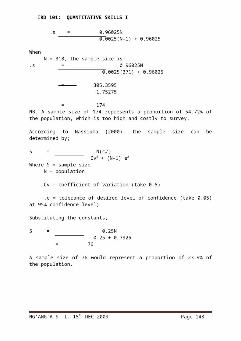
IRD 101: QUANTITATIVE SKILLS I
7. 0 TIME SERIES: (8 HOURS)7.1 Definition of time series concepts
7.2 Examples of time series
7.3 Moving averages
7.4 Estimation of trend,
- Use of scatter diagrams.
7.1 Definition of Time series graphs In a times series, values of a variable are given at a different periods of time. When a graph of
such a series is drawn it would give changes in the value of a variable with the passage of
time. The graphical presentation of such a series is called a histogram.
The aim of drawing such graphs is to have comparison to study the
(i) Changes in one variable over a period of time and
(ii) Changes if two or more variables over a period of time.
While constructing a histogram, time is taken along x – axis and the values along y – axix
then the data is plotted and points are joined by means of straight lines to get the histogram.
The main examples of time series are as under;-
a) Population of a country over a specific period of time.
b) Sales of a business enterprise over a period of one year.
c) Prices of some specific commodities over a period of time
d) Temperature over a period of time.
Example 3:
Monthly sales of AB stores for the year 19 – 8 were as follows:-
Month Jan Feb Mar Apr May Jun Jul Aug Sept Oct Nov Dec
Sales
(shs
000)
50 40 60 70 50 80 100 90 110 80 70 120
NG’ANG’A S. I. 15TH DEC 2009 Page 143
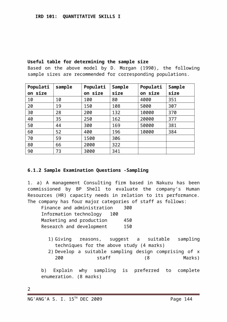
IRD 101: QUANTITATIVE SKILLS I
Construct a graph from the above figures.
Example 4
The following table gives the sales of a certain firm in 6 – years. Draw a graph of time series.
Years 1991 1992 193 1994 1995 1996
Sales Sh.
(000’s)
820 950 1000 950 900 1050
In this graph, false base line is required. When the fluctuations in a variable are relatively
small to its size then a definite break in the scale is shown between zero and the next number.
in this case, instead of showing the entire scale from zero to t
he highest value involved. Only as much is shown as is necessary for the purpose. The
portion which lies between zero and the lowest value of the variable is left out. This method
is termed as False Line Approach Showing time series graphs.
- Economists and businessmen have the task of making estimates about the future so that they
can be able to plan for various things such as:
- Sales
- Production
- Food supply
- Jobs for the people
NG’ANG’A S. I. 15TH DEC 2009 Page 144

IRD 101: QUANTITATIVE SKILLS I
- Technology needs etc
- However, the step in making these estimates encompasses gathering information from the
past, which means that one deals with statistical data collected, observed, or recorded at
successive intervals of time. Such data are generally referred to as time series.
- Thus, when numerical data is observed at different points of time creates a set of
observations known as time series. Different points of time means over 5 years, 10 yrs, 20 yrs
etc.
- suppose production sales, exports, imports etc is observed at different points of time, say
over 5 or 10n yrs, the set of observations formed constitutes time series. Hence in the analysis
of time series time is very important because variable is related to time.
NB: time series refer to statistical data arranged chronologically, over successive increments,
in order of their occurrence etc.
Example: the data below shows sales of Radios by a firm in ‘000’ units:
Year sale of Radios (000)
1999 40
2000 42
2001 47
2002 41
2003 43
2004 48
2005 65
2006 42
- Observing the above series reveal that generally the sales have increased but for two
years a decline is also noticed.
7.2 Components of a time series- The statistical analysis the effect of the various forces on data under 4 broad
categories.
1. Secular movements: which refer to those changes that have occurred as a result of
general tendency of the data occurred or occurred. Secular trends do not include short
NG’ANG’A S. I. 15TH DEC 2009 Page 145
IRD 101: QUANTITATIVE SKILLS I
range movements but rather steady movements over along time. They are attributable
to factors such as population change, technological progress, large scale shift in
consumer tastes etc all which would lead to rising or falling trends in prices,
production, sales, incomes, employment, demand for food, clothing, shelter, discovery
and exhaustion of natural resources, mass production methods, improvement in
business organization etc. they cause, major growth or decline in time series.
- sometimes a growth in one series involves a decline in another e.g. the displacement
of skin clothes by cotton clothes, better medical services have reduced death rates but
then contributed to rise in birth rates etc.
- Also some series increase slowly and some increase fast. Others decrease at varying
rates; some remain relatively constant for long periods of time etc.
2. Seasonal variation: Which concerns changes that have taken place during a period of
12 months as a result of change in climate, weather conditions, festivals etc? They are
periodic movements in business activity occurring regularly every year as a result of
the nature of year itself. The variations repeat during a period of 1 year hence they can
be predicted fairly accurately factors known to cause seasonal variations include (a)
Climate and weather conditions e.g. which lead to climate or climate DD for woolen
clothes, hot drinks, cold drinks, planting season, harvest season etc. (b) customs,
traditions and habits e.g. Christmas leading to large for clothes, wheat flour, showers,
etc, money (withdrawals, etc.
3. cyclical variations:- which concern changes that have taken place as a result of booms
and deforestations. They are recurrent variations that cast longer than one year are
regular neither in amputable nor in length. Time series, mostly in economics and
businesses, fall under this category. They are known as business cycles which have
four phases:
1. Prosperity
2. decline
NG’ANG’A S. I. 15TH DEC 2009 Page 146

IRD 101: QUANTITATIVE SKILLS I
3. deforestation
4. recovery
4. Irregular variations: also called erratic, accidental or random. This category concerns
changes that have taken place as a result of such forces that could be predicted like
floods, earthquakes, famines etc. these business variations do not recur in a definite
pattern. These variations include: all those others except those particularly scanter
trend, seasonal and cyclical variations have certain systematic movements e.g. sudden
fall in DD or rafoid technological movements can be included in this category.
NB: that the four variations explained above are also known as the components of time series.
Each of these components can be measured. However for this course we shall only measure
secular variations (trend).
Measuring trend
This is the determination and presentation of the direction which any long term series takes
i.e. is it growing or declining. Key reasons for measuring trend include:
1. To find trend characteristics about a given variable eg comparing the growth
of textile sector in Kenya with that of other countries, the growth of textile
sector in Kenya with that of the whole country.
2. To eliminator trend so as to study other components of time series such as
seasonal, cyclical and irregular variations.
Methods of measuring trend
1. Free hand smoothing or the graphic method
2. semi averages method
3. moving averages
4. Least squares method.
1. Free hand smoothing/ Graphic method
NG’ANG’A S. I. 15TH DEC 2009 Page 147
3
2 4
1
3
4

IRD 101: QUANTITATIVE SKILLS I
It’s the simplest method of studying trend. The following procedure is followed
(a) Plot the time series on the graph.
(b) Examine the direction of the trend based on the plotted dots.
(c) Draw a straight line which will best fit to the data according to person’s judgment.
The line shows the direction of the trend.
Example: Fit a trend line to the following data by the free hand method
Year production of steel (in millions)
1990 20
1991 22
1992 24
1993 21
1994 23
1995 25
1996 23
1997 26
1998 25
Fitting by free hand method
NG’ANG’A S. I. 15TH DEC 2009 Page 148
The trend line can be extended to predict future values. But since the free hand curve fitting is too subjective, this method should not be used for predictions
Trench line
25
24
23
22
21
20
Actual data
91 92 93 94 95 96 97 98
Prod
uctio
n
Years
IRD 101: QUANTITATIVE SKILLS I
The trend like can be extended to predict future values. But since the free hand curve fitting is
too subjective, this method should not be used for predictions
7.3 Method of semi averages- When this method is used, the given data is divided into two parts, preferably with the same
No. of years.
- Then SAM of each part is taken/ calculated so that two points are obtained which are
plotted at the mid point of the class interval covered by the respective part and then the two
points are joined by a straight line. This straight line gives the needed trend line. The line can
be extended gives or gives to get intermediate value or predict future values.
Example: fit trend line to the following data by a method of semi – averages.
Year sales of firm A (in thousand units)
1992 102
1993 105
1994 114
1995 110
1996 108
1997 116
1998 112
NB: since 7 years are given, the middle year shall be left out and an average of the first three
years be obtained. The average of first three years is;
102 + 195 +114 = 321 = 107
3 3
Average of last three years is
108 + 116 +112 = 336 = 112
3 3
Thus two points 107 and 112 will be gotten and plotted correspondingly to their respective
middle years i.e. 1993 and 1997. Plotting these points we get the needed trend line. The line
can be extended to predict or determine intermediate values.
NG’ANG’A S. I. 15TH DEC 2009 Page 149

IRD 101: QUANTITATIVE SKILLS I
NB: Where there even Number of years, two equal parts can easily be obtained. Hence, given
the years 1990, 91,92,93, 94, 95, 96, 97, the first part of years would be 90, 91, 92, 93 and the
second part would be 94, 96, 97, 98. The centering of the averages each part would be
between 91 and 92 for 1st part and 96 and 97 for second part.
Procedure:
1. Plot the actual data
2. divide data in two parts
3. get and plot the averages
4. connect the two points to get the trend line
3. Method of moving averages:
When trend is determined by this method, the average value for a number of years is secured.
It is therefore necessary to select the period of the moving average such as three yearly
moving averages; five yearly moving averages, 8 yearly moving average etc. the length of the
cycle determines the period of moving average. For instance, a 3 yearly moving average shall
be computes as follow;
a+ b + c; b + c + d ; c + d+ e; d + e + f ; etc
3 3 3 3
NG’ANG’A S. I. 15TH DEC 2009 Page 150
Trend line
Actual data
93 94 95 96 97 98 99 0091992
105
110
115
120
125
130
135
Sale
s
Years
100

IRD 101: QUANTITATIVE SKILLS I
Five yearly moving averages shall be;
a+ b + c +d + e; b + c + d +e +f ; c +d + e +f + g ; etc
3 3 3
Examples:
(a) Using a three year moving averages determine the trend and short term fluctuations.
Plot the original and trend values on the same graph paper
Year production (‘000’ tones)
1989 21
1990 22
1991 23
1992 25
1993 24
1994 22
1995 25
1996 26
1997 27
1998 26
Graph of original trend values of products by moving averages methods
NG’ANG’A S. I. 15TH DEC 2009 Page 151
years1989 90 91 92 93 94 95 96 97 98
22
24
26
28
30
20
96
Trend line
Actual data
Prod
uctio
n

IRD 101: QUANTITATIVE SKILLS I
Sol.
Year prod. 3 yr moving 3 yr moving short term
(ooo tons) totals averages (fluctuation y1 – yc)
1989 21 - - -
1990 22 66 22.00 0
1991 23 70 23.33 -0.33
1992 25 72 24.00 +1.00
1993 24 71 23.67 + 0.33
1994 22 71 23.67 - 1.67
1995 25 73 24.33 + 0.67
1996 26 78 26.00 0
1997 27 79 26.33 + 0.67
1998 26 - - -
Graph of original and trend values of product by moving averages method
b) Calculate 5 yearly moving averages for the following data.
Year product
1986 105
1987 107
1988 109
1989 112
1990 114
1991 116
1992 118
1993 121
1994 123
1995 124
1996 125
1997 127
1998 129
Sol.
Year prod. 5Yrly totals 5 yrly M.A
NG’ANG’A S. I. 15TH DEC 2009 Page 152

IRD 101: QUANTITATIVE SKILLS I
1986 105 - -
1987 107 - -
1988 109 547 109.4
1989 112 558 111.6
1990 114 560 113.8
1991 116 581 116.2
1992 118 592 118.4
1993 121 602 120.4
1994 123 611 122.2
1995 124 620 124.0
1996 125 628 125.0
1997 127 - -
1998 129 - -
Then, plot both the actual and moving averages data.
Even period of moving average:
If the moving average is an even period average say, 4 yearly or 6 yearly, the moving total
and moving averages are placed at the centre of the time span from which they are computed.
This placement is inconvenient since the moving averages so placed does not coincide with
the original time period. The two would then be synchronized i.e. moving averages and the
original data by process called centering which consists of taking a two period moving
average of moving averages.
Example:
Year value
1985 12
1986 25
1987 39
1988 54
1989 70
1990 87
1991 105
1992 100
1993 82
1994 65
NG’ANG’A S. I. 15TH DEC 2009 Page 153
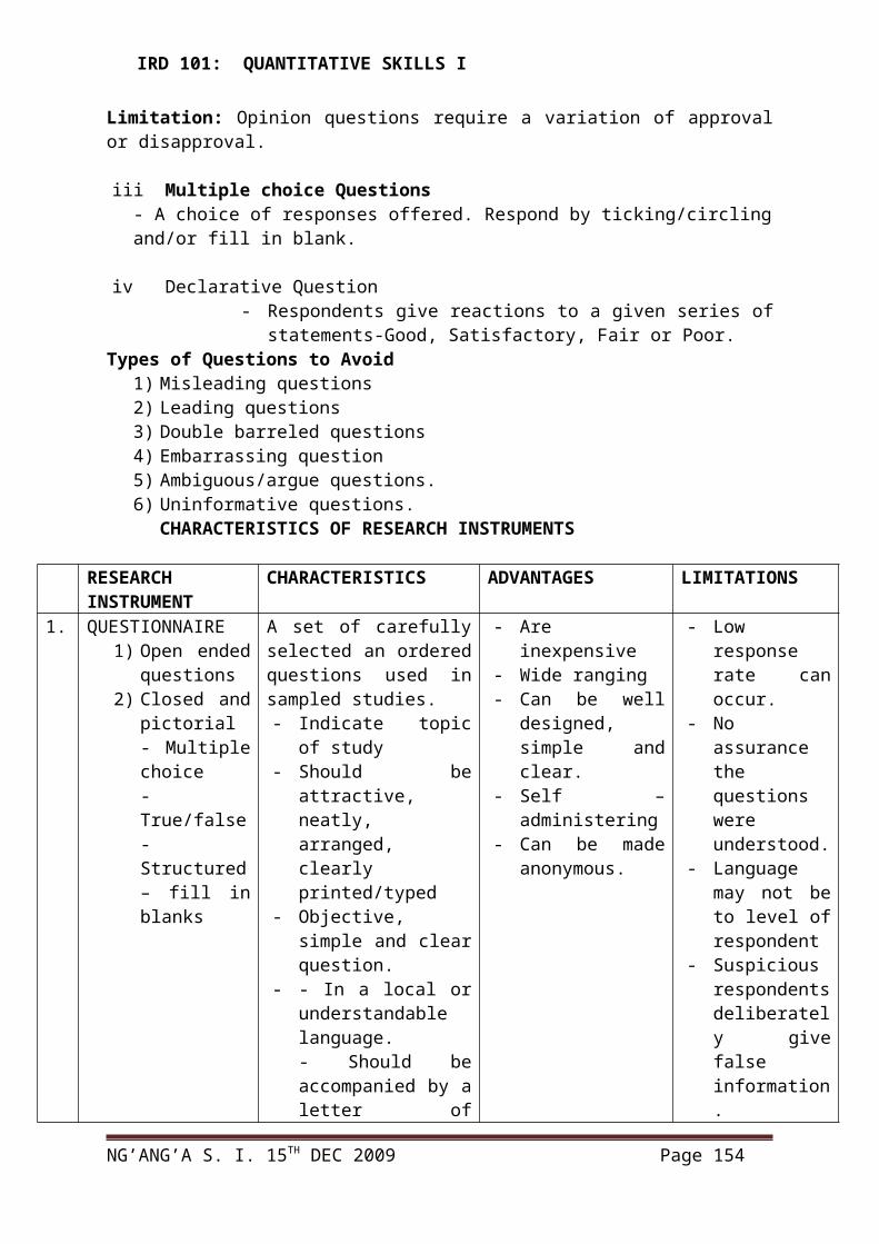
IRD 101: QUANTITATIVE SKILLS I
1995 49
1996 34
1997 20
1998 7
Sol.
Yr value 4y.M.T 4 M.A. 4y centered M.A
1985 12 - - -
1986 25 - - -
130 32.5
1987 39 39.75
188 47.0
1988 54 54.75
250 62.5
1989 70 70.75
316 79.0
1990 87 84.75
362 90.5
1991 105 92.00
374 93.5
1992 100 90.75
352 88.0
1993 82 81.00
29.6 74.0
1994 65 65.75
230 57.5
1995 49 49.75
168 42.0
1996 34 34.75
110 27.5
1997 20
1998 7
Then plot the actual data and the 4 yrly centered moving averages.
NG’ANG’A S. I. 15TH DEC 2009 Page 154

IRD 101: QUANTITATIVE SKILLS I
Exercise
From the following data compute 3 yrly, 5 yrly and 7 yrly moving averages and plot them on
the graph paper with the actual data.
Year: 1984 85 86 87 88 89 90 91 92 93 94 95 96 97 97
+2 +1 0 -2 -1 +2 +1 0 -2 -1 +2 +1 0 -2 -1
Yr fluctuations 3 M.A 5 M.A 7 M. A.
1984 +2 - - -
85 +1 +1.00 - -
86 0 -0.33 0 -
87 -2 -1.00 0 +0.43
88 -1 -0.33 0 +0.14
89 +2 +0.67 0 -0.28
90 +1 +1.00 0 -0.43
91 0 -0.33 0 -0.14
92 -2 -1.00 0 -0.43
93 -1 -0.33 0 +0.14
94 +2 +0.67 0 -0.27
95 +1 +1.00 0 -0.43
96 0 -0.33 0 -
97 -2 -1.00 - -
98 -1 - - -
7.4 Method of least squares:This method is most widely used in practice. It’s a mathematical method and with its help a
trend line is fitted to the data in such a manner that the following two conditions are satisfied:
1. ∑ (Y – Yc) = 0 sum of deviations of the actual values of Y and the confronted values
of Y is zero.
2. ∑ (Y – Yc) 2 is least: i.e. the sum of the squares of the deviations of the actual and
computed value is least from this line and hence the name method of least squares.
The line of best fit.
This method of least squares is used to fit straight trend line or a paragraphed trend. The
straight line is represented by the equation Yc = a + bx
NG’ANG’A S. I. 15TH DEC 2009 Page 155
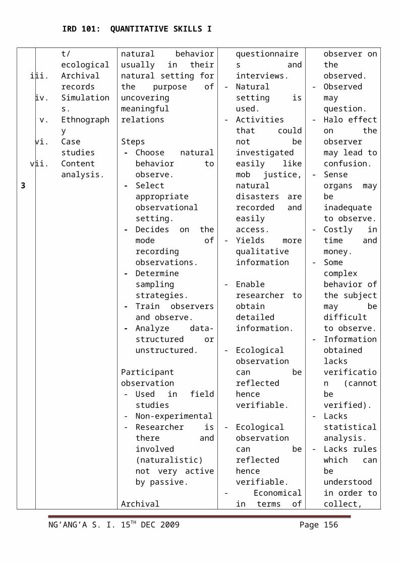
IRD 101: QUANTITATIVE SKILLS I
Where Yc = The trend/ confronted values
a= Y Intercept
b= slope/ gradient of the trendline
x= the variable which represents time
In order to determine the values of the constants a and b the following two normal equations
are to be solved.
∑Y = Na + B∑ X……………….(i)
∑XY = a∑X +b∑x2…………….(ii)
Where N represents the number of years for which data are given. Two approaches;
Approach i
The variable X can be measured from any point of time in origin such as the first year. But
calculations are very simplified when the mid-point in time is taken as the origin because in
that case the –ve values in the half of the series balance out the +ve values in the 2 nd half so
that ∑ X = 0. The variable is measured as a deviation from its mean.
Since ∑X = 0
∑ Y = Na the value of a and b can be determined easily.
∑ XY = b∑X2
Since ∑ Y = Na therefore a = ∑Y/ N
∑XY = b ∑x2 therefore b = ∑XY/
∑x2
Example:
Below are data of figures of production in tones from a factory.
Year: 1992 1993 1994 1995 1996 1997 1998
Production: 80 90 92 83 94 99 92
Required: (i) Fit a straight line trend to these figures
(ii) Plot these figures on a graph and show the trend line.
NG’ANG’A S. I. 15TH DEC 2009 Page 156
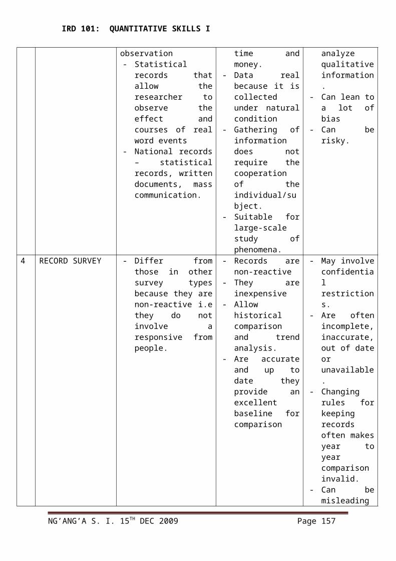
IRD 101: QUANTITATIVE SKILLS I
Solution (i) NB:1995 is taken as origin
Year production X XY X2 Yc = a + bx
Trend values
1992 80 -3 -240 9 84
1993 90 -2 -180 4 86
1994 92 -1 -92 1 88
1995 83 0 0 0 90
1996 94 +1 +94 1 92
1997 99 +2 +198 4 94
1998 92 +3 +276 9 96
N= 7 ∑Y = 630 ∑X = 0 ∑XY = 56 ∑XY2 = 28 ∑Yc = 630
The equation of a straight line trend is Yc = a + bx
Since ∑X = 0
a= ∑Y/N; b = ∑XY/∑X2
But: ∑Y = 630; N = 7; ∑XY = 56; ∑X2 = 8
a= 630/ 7 = 90; b = 56/28 = 2
Hence the equation of the straight line trend = Yc = 90 + 2x
Thus trend values (yc) for each year would
1992: Yc = 90 + 2 (-3)
= 90 + -6
= 90- 6 = 84
1993: Yc = 90 +2 (-2)
= 90 + - 4
= 86 etc
NG’ANG’A S. I. 15TH DEC 2009 Page 157

IRD 101: QUANTITATIVE SKILLS I
Linear trend method by least squares
Suppose you took 1992 as the origin, the values of X will all be +ve after zero of 1992. ∑X =
218 not zero. Hence;
630 = 7a + 21b
1946 = 21 a + 91 b
The equation fitting trend line will change to Yc = 84 + 2x. the difference in origin. However
the trend values will be the same.
Example:
(a) Fit a straight line trend for the following series
(b) Estimate the value for 1999
(c) What is the monthly increase in production?
Year: 1992 1993 1994 1995 1996 1997 1998
Production: 125 128 133 135 140 141 143
Sol
NG’ANG’A S. I. 15TH DEC 2009 Page 158
75
80
85
90
95
100
93 94 95 96 97 981992
Actual data
Trend lines
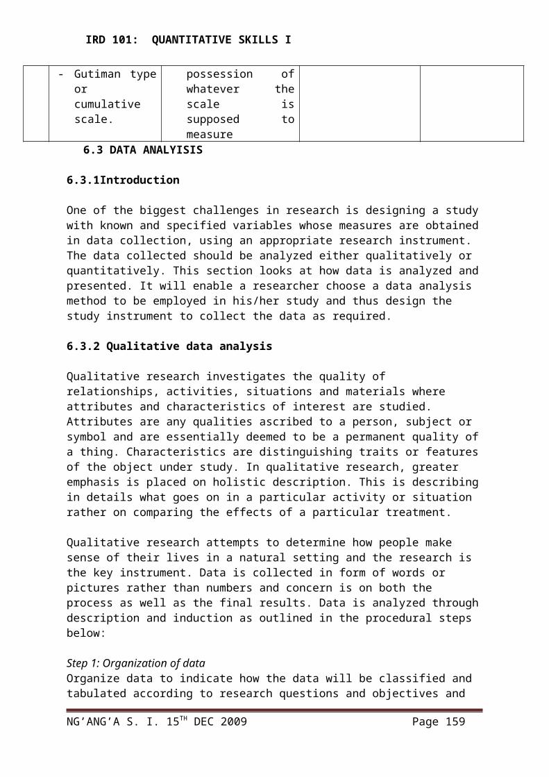
IRD 101: QUANTITATIVE SKILLS I
Year production X XY X2 Yc= a+bx
1992 125 -3 -375 9
1993 128 -2 -256 4
1994 133 -1 -133 1
1995 135 0 0 0
1996 140 +1 +140 1
1997 141 +2 +282 4
1998 143 +3 +429 9
N=7 ∑Y=945 ∑X=0 ∑XY=87 ∑X2=28
The equation of the straight line trend is
Y = a +bx
Since ∑X = 0 a = ∑Y/N = 945/7 = 135
b= ∑XY/∑X = 87/28= 3.107
Hence: Yc = 135 + 3.107X
(b) For 1999 X will be + 4 thus Y 1999 = 135 + 3.107 (4)
= 147.428 tons
(c) Given the equation Yc = a+bx; b is the rate of change (in production) and in our trend
equation Yc = 135 + 3.107x the (annual) rate of change is 3.107 million tons. This monthly
increase would be given by 3.107/12 = 0.25 tons.
Example: using the method of least squares fit a trend line to the following data and find the
trend values and short term fluctuation.
NG’ANG’A S. I. 15TH DEC 2009 Page 159

IRD 101: QUANTITATIVE SKILLS I
Year: 1990 1991 1992 1993 1994 1995 1996 1997 1998
Value: 232 226 220 180 190 168 162 152 144
Sol.
Year value(Y) X XY X2 Yc short term -
Fluctuation (Y – Yc)
1990 232 -4 -928 16 232.8 -0.8
1991 226 -3 -678 9 221.1 +4.9
1992 220 -2 -440 4 209.4 +10.6
1993 180 -1 -180 1 197.7 -17.7
1994 190 0 0 0 186.0 +4.0
1995 168 +1 +168 1 174.3 +6.3
1996 162 +2 +324 4 162.6 -0.6
1997 152 +3 +436 9 150.9 +1.1
1998 144 +4 +576 16 139.2 4.8
N=9 ∑Y=1674 ∑x=0 ∑XY=702 ∑x2=60 ∑Yc =1674
Y = a + b x
a = ∑Y/N = 1674/9 =186
b= ∑xY/∑x2 = -702/60 = -11.7
Hence Y = 186 11.7x
Y1990 = 186 -11.7(-4) = 186 + 46.8 = 232.8 = 232.8
Approach iiTo obtain the regression equation y = a + bx values of a and b are obtained from
a =
b =
Which are derived from solving the simultaneous equations
an + bx = y…………………………………….(i)
NG’ANG’A S. I. 15TH DEC 2009 Page 160
IRD 101: QUANTITATIVE SKILLS I
ax + bx2 = xy ………………………………...(ii)
The data obtained for x & y is tabulate to get the sums x, y, xy and x2 as follows.x....
y....
x2
.
.
.
.
Xy....
x y x2 xy
Note: (i) The line obtained can be extended and used to predict (forecast).
(ii) If the gradient or slope is negative (i.e. b is positive) the two variables x and y have
a positive relationship and y increases as x increases.
(iii) If the gradient (slopes) in negative (b is negative) the two variables have a negative
relationship and y decreases as x increases.
Example
Example Period Actual demand Forecasts1234567
648747-
-6566.257.25-
Forecast demand for period F7
From the example above, when the period stands for the independent variable x and actual
demand stands for the dependent variable y, the values a and b and the regression equation
are calculated as follows.
x123456-
y648747-
x2
149162536-
xy6824282042-
x=21 y=36 x2 =91 xy =128
NG’ANG’A S. I. 15TH DEC 2009 Page 161
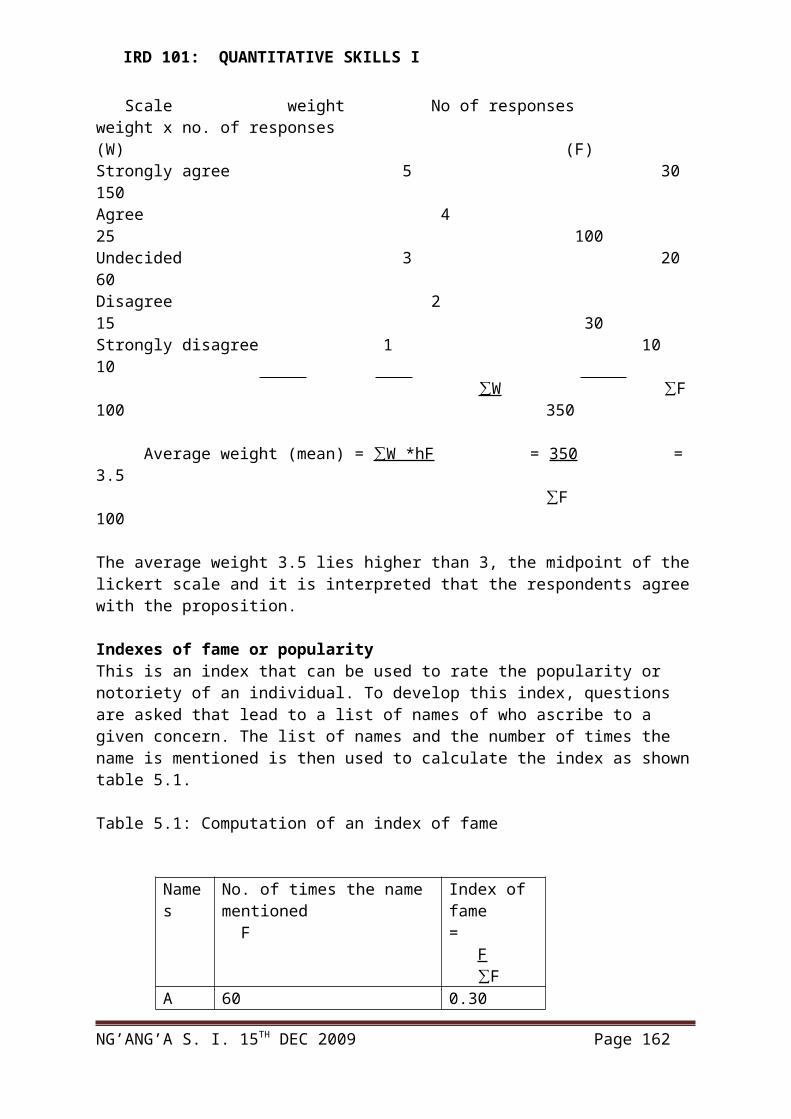
IRD 101: QUANTITATIVE SKILLS I
From which,
b =
= = = 0.114
From which,
a =
= = = 5.601
This gives a regression Equation of
Y = a + bx
Y = 5.601 +0.114x.
The regression equation suggests a demand that increases slightly with increase in time and
may lead to a forecast for period 7 of;
Y = 5.601 + 0.114(7) = 6.40
7.4Revision questions1.Explain four factors that might lead to a random variation in Kenya tea exports over a period of one year. 4mks 2. Indicate the time series movement you will associate with the following events
i. Resistant of malaria parasite to quinine 1mkii. Presidential and parliamentary elections in Kenya after every five years
1mkiii. Fire outbreak at petrol filling stations 1mk
3. a) Explain why a supermarket may want to analyze the time series data it generates in its sales 4mks b.) The following time series data shows the annual production of sugar at a local sugar processing firm in western Kenya or the years 1997-2005
NG’ANG’A S. I. 15TH DEC 2009 Page 162

IRD 101: QUANTITATIVE SKILLS I
Year Production (000 tonnes )1997 201998 221999 242000 212001 232002 252003 232004 262005 25
Required i.) Determine the trend lien using the method of centered moving average of order 4
6mks ii.) on the same axes, plot the time series data and the trend line obtained in i.) above
4mksiii.) Using the graph obtain estimates of sugar production for the firm for the years 2006 and 2007 4mks
4.With which characteristic movement of a time series would you mainly associate each of the following independent cases or situations?
i.) An increase in sales for a supermarket during Christmas 1mkii.) The decline in the spread of HIV/AIDS in Kenya 1mkiii.) The university lecturers union strike 1mkiv.) A continually increasing demand for new information technology
1mkv.) The heavy rains that caused floods in Kenya in November/December 2006
1mk
5. a) Explain the meaning of the following terms;i.) Time series
ii.) Raw data iii.) Median iv.) Sample
12mks b.) The table below gives the production figures (in 000 of tonnes) of ceramic goods for
2006. Month Jan Feb Mar Apr May Jun July Aug Sep Oct Nov Dec Production 335 325 310 354 360 338 333 270 375 395 415 373
iv.) Plot the monthly production figures on a graph 5mksv.) Which time series factor seems to influence the production of ceramic
goods? 3mksvi.) Use the graph to estimate the production figures for the ceramic good in
February 2007. 4mks
6. (a) List and illustrate four components of a time series (4marks)
NG’ANG’A S. I. 15TH DEC 2009 Page 163
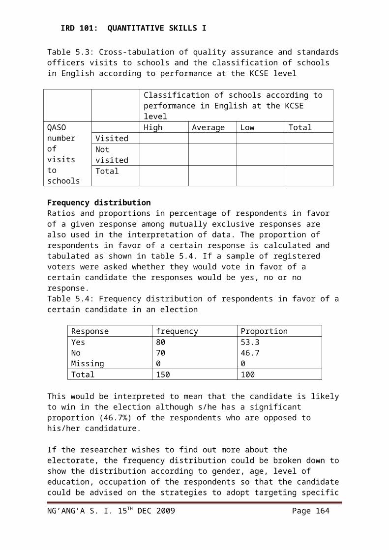
IRD 101: QUANTITATIVE SKILLS I
(b) A firm has recorded the following sale data in (000)Year Time Sales1998 1 41999 2 22000 3 82001 4 122002 5 202003 6 182004 7 162005 8 302006 9 402007 10 362008 11 44
From the above data;(i) Plot a scatter graph of time against sales (2marks)(ii) Find a trend line using the least square method (3marks)(iii) Plot the least square trend line on the same graph (i) above (2marks)(iv) Using the least square trend line, determine the sales forecast for year 2009 and
2010 (2marks) 7. The table below gives the production figures (in 000 of tones) of ceramic goods for 2006. Month Jan Feb Mar Apr May Jun July Aug Sep Oct Nov Dec Production 335 325 310 354 360 338 333 270 375 395 415 373
i.) Plot the monthly production figures on a graph 5mksii.) Which time series factor seems to influence the production of ceramic
goods? 3mksiii.) Use semi averages to plot a trend line on the graph and use it to estimate the
production figures for the ceramic good in February 2007. 4mks
iv.) Use the least squares method to plot a trend line on the same graph and estimate production figures for Feb 2007.
v.) Which of the two methods do you think is more accurate and why?The table below gives the production figures (in 000 of tones) of ceramic goods for 2006. Month Jan Feb Mar Apr May Jun July Aug Sep Oct Nov Dec Production 335 325 310 354 360 338 333 270 375 395 415 373
i.) Plot the monthly production figures on a graph 5mksii.) Which time series factor seems to influence the production of ceramic
goods? 3mksiii.) Use semi averages to plot a trend line on the graph and use it to estimate the
production figures for the ceramic good in February 2007. 4mks
iv.) Use the least squares method to plot a trend line on the same graph and estimate production figures for Feb 2007.
v.) Which of the two methods do you think is more accurate and why?8. a) Explain the following components in time series analysis
i.) Seasonal variationii.) Random variationiii.) Cyclic variation
NG’ANG’A S. I. 15TH DEC 2009 Page 164

IRD 101: QUANTITATIVE SKILLS I
b.) A firm has recorded the following levels of production in the last seven years.Year 2002 2003 2004 2005 2006 2007 2008Production 125 128 133 135 140 141 143
Required i.) Using the three years moving average calculate the projected level of production
for the year 2009.ii.) Plot a scatter graph for the data iii.) Fit a straight line trend for the data.iv.) Use the trendline to predict production levels for the year 2009.v.) Comment on the production level estimated by the moving average methods and
the trendline for the year 2009.9. The annual DAP fertilizer consumption in thousands of tonnes during 1995-2001 in Lukuyani Division was recorded as given below.Year 1995 1996 1997 1998 1999 2000 2001Consumption (‘000) tonnes
50 56 60 68 70 75 78
a.) i.) Use the semi average method to fit the trend line and use it to estimate the consumption in 2005. 12mksii.) Indicate two major disadvantages of this method 4mks10. a) Explain
i.) The meaning of time series analysis 2mks
ii.) The importance of time series analysis 2mks
b)List and illustrate four components of time series (4mks)
c)A firm has recorded the following sales data in (000)
Year Time Sales
1998 1 4
1999 2 2
2000 3 8
2001 4 12
2002 5 20
2003 6 18
2004 7 16
2005 8 30
2006 9 40
2007 10 36
2008 11 44
Form the data above
i.) Plot a scatter graph of time against sales
3mks
NG’ANG’A S. I. 15TH DEC 2009 Page 165
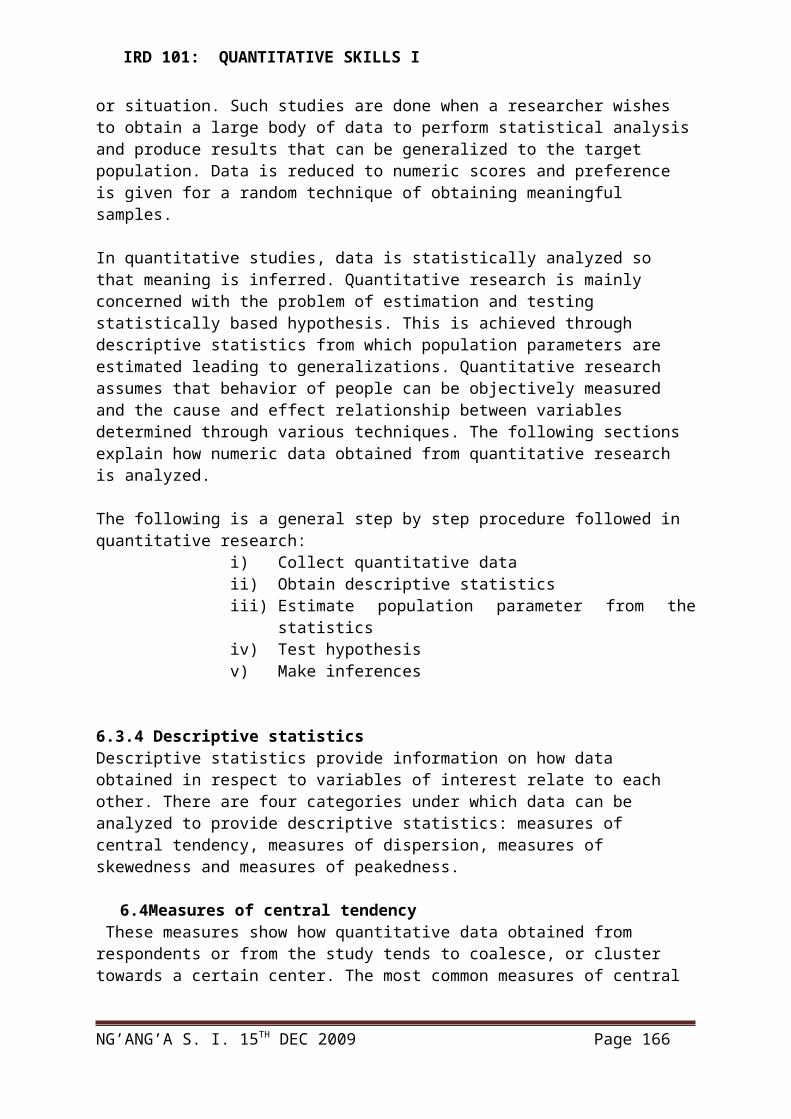
IRD 101: QUANTITATIVE SKILLS I
ii.) Use semi averages to plot a trend line on the scatter plot in i.) above
2mks
iii.) Using the trend line forecast sales for the year 2009 and 2010
2mks
iv.) Find the trend line using the least squares methods 3mks
v.) Plot the least square trend line on the same graph i.) above 2mks
vi.) Using the least squares trend lines determine the sales forecast for year
2009 and 2010 2mks
vii.) Comment on the forecast by semi average trend line iii.) Above and those
by least squares trend line (vi.). 2mks
NG’ANG’A S. I. 15TH DEC 2009 Page 166
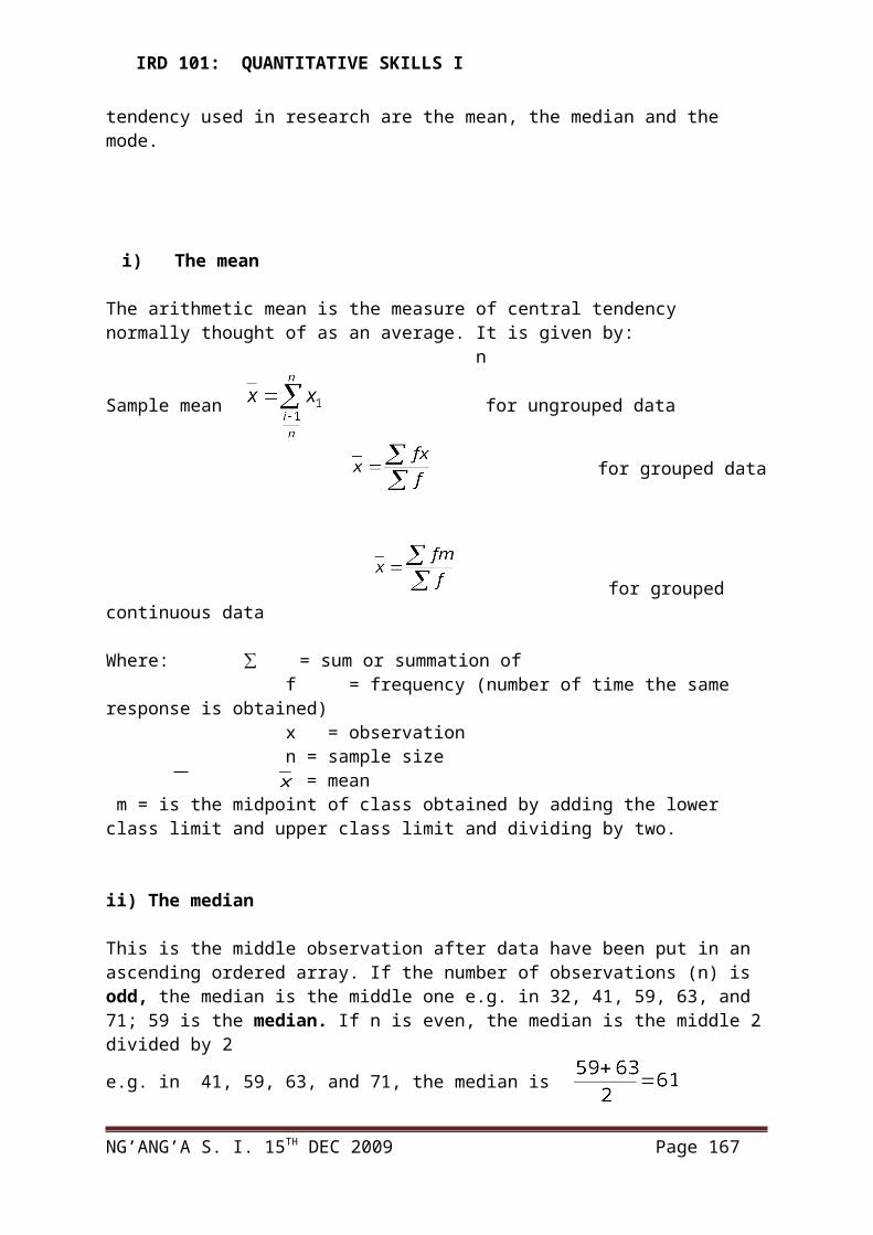
IRD 101: QUANTITATIVE SKILLS I
FORMULAE COMMOINLY USED IN IRD 101
1. Arithmetic mean
2. Median of grouped data
3. Mode of grouped data
4. Standard deviation
5. Coefficient of variation
6. Regression line of y on x Y= a+bx
NG’ANG’A S. I. 15TH DEC 2009 Page 167

IRD 101: QUANTITATIVE SKILLS I
NG’ANG’A S. I. 15TH DEC 2009 Page 168