READING LIST ON ECONOMIC GROWTH

Topics and readings:The main text is Auerbach, A., and L. Kotlikoff, “Macroeconomics-An integrated Approach”, 2nd edition, MIT Press.Other required readings are journal articles, which are available on the course web.Also chapters in Mankiw’s intermediate macroeconomics text, and a chapter in Varian’s Intermediate Microeconomics text should be read.

0. Review of National Income AccountingMankiw, ch. 2 and handout below, read by yourselves

1. The neoclassical production function and factor markets.Required reading: Auerbach and Kotlikoff (AK), chapter 1; Mankiw; ch.3 (supply); handout.

2. Review and in-depth analysis of the Solow-model.Required reading: Mankiw, chapters 7-8; Handout.

Extra-credit exercise: simulation exercise of the Solow-model to be handed in.

3. Empirics of Economic GrowthRequired reading: Two journal articles available on the course-web:

J. Persson, Convergence across the Swedish Counties 1906-1993, European Economic Review, 1997, eer.pdf

R. Barro, Human Capital and Economic Growth, Swedish Economic Policy Review, growthbarro.pdf

Students not previously exposed to econometrics should read the summary of econometric methods provided on the course web.

Students should do econometric exercise and write econometric report.For C-students this exercise is an extra credit exercise; for D-students it is required.

In addition, D-level students should do additional report related to economic growth or to the course in general. It could e.g. be that students include an additional explanatory variable in the regressions related to the empirical growth exercise mentioned above.

4. Endogenous growth modelsRequired reading: Mankiw, ch. 8; and handout below.

5. Income distribution and Economic Growth.Article on income inequality and economic growth by Robert Barro.Perhaps class-room presentation of D-level student(s).

6. Pollution and Economic Growth.Persson (2008), to be added on the course web.

7. The overlapping generation model (OLG)A. Optimal consumption, and saving by a young person.AK: chapter 2.B. More in-depth analysis of saving.Required reading: Mankiw, Chapter 17 and handout below. C. Endogenous labor supply.Required reading: Handout below (based on the textbook by Varian).

D. Completing the OLG-model.AK, Ch. 3

8. Review of National Income AccountingAK, chapter 5.

9. A government sector in the OLG-model.AK, chapter 6; Handout below; Mankiw, government debt: ch. 15 (relevant parts)

10. Factor mobility in the OLG-model: An analysis of globalization. AK, ch. 12.

11. Precautionary saving in the OLG-model. AK, ch.15; Handout below; Mankiw, government debt: ch. 15 (relevant parts)

There may be other topics as well and a couple of additional articles if we have time.Maybe not:12. Fertility Choice and Income level.Reading: handout below.

CH. 2 (Mankiw): National Income Accounting MEASURING PRODUCTION AND INCOMEGross domestic product (GDP) is the market value of all final goods and services produced within an economy during a year.In Swedish: Bruttonationalprodukt (BNP) till marknadspris

GDP can be measured in 3 ways:Method 1. through expenditures on final goods and services.Method 2. through income (wages and capital income).Method 3. through production. GDP is calculated by adding up value added in all sectors of production. Value added = total revenue – expenditures on inputs other than capital and labor. These inputs are intermediate goods (insatsvaror). In Swedish:BNP till marknadspris kan mätas från:

1. Utgiftssidan. 2. Inkomstsidan. 3. Produktionsidan.

In an economy without a government sector and without international trade (Exports=imports=0).

HOUSEHOLDS supply the factors of production (capital and labor) to FIRMS which use these factors of production to produce final goods and services that are sold to the HOUSEHOLDS.

Households supply the factors of production (capital and labor) to the firms. In other words, the households own the firms. Firms use factors of production to produce final goods and services that are sold to the households.The households’ expenditures on final goods and services equals factor incomes (wages, interest, profit) from the firms in this economy.

There are 2 ways of viewing GDP

Total income of everyone in the economy

Total expenditure on the economy’s output of goods and services

There are 2 ways of viewing GDP

Total income of everyone in the economy

Total expenditure on the economy’s output of goods and services

Households Firms

Income $

Labor

Goods

Expenditure $

Households Firms

Income $Income $

LaborLabor

GoodsGoods

Expenditure $Expenditure $

For the economy as a whole, income must equal expenditure. GDP measures the flow of dollars in this economy.

Income, Expenditure And the Circular FlowIncome, Expenditure And the Circular Flow

Example of method 3; that is, measuring GDP by adding up value added in the different sectors of production. Assume one final good in the economy, bread:Sector: Total revenue=

P*QCost of inputsOther than KAnd L

Value Added

Capital andLabor income

Peasant: Wheat 100 0 100 100Miller: flour 150 100 50 50Baker: bread 200 150 50 50Sum: 200 200Method: 1 3 2

Compute GDP in current prices (BNP till marknadspris i löpande priser) according to method 1. Assume two goods in the economy:

Comparing standard of living across time

Nominal and real GDP: GDP in current and constant pricesIn Swedish: BNP till marknadspris i löpande och fasta priser.

The value of final goods and services measured at current prices is called nominal GDP. It can change over time either because more goods and services are produced or because there is a change in the prices of these goods and services.

We calculate real GDP to see whether the country is producing more or less goods and services over time.

Real GDP 2000 (in 2000 year prices) = nominal GDP 2000.Real GDP 2001 (in 2000 year prices) =

If real GDP 2001 > real GDP 2000, then the economy produced more goods and services in 2001.Often in news papers and statistical reports you get data on GDP in current prices and data on a price index. How do we calculate GDP in constant prices?

Real GDP in 2005 (in 2000 year prices) = nominal GDP in 2005/ price index in 2005

Year Nominal GDP=GDP in currentPrices

Price index =GDP-deflator

Real GDPin 2000 year prices

2000 2500 billion kr 100 25002001 2600 billion kr 102 2600/1.02=25492002 2700 billion kr 104 2700/1.04=25962003 2800 107 2800/1.07=26162004 2900 110 2900/1.10=26362005 3000 112 3000/1.12=26782006 3100 114 3100/1.14=2719

Thus, real GDP increases by = 0.088, by 8.8 %

Between year 2000 and 2006.

Calculating the same using an approximate formula:

1.2 percent difference between the exact and the approximate formula.

Real wage = nominal wage / price levelIf the nominal wage in percentage terms increases more than the price level increases, then the real wage increases, which means that you can buy moregoods and services: your purchasing power increases.

More rules for computing GDP:2) used goods are not includes in the calculation of GDP.3) If newly produced final goods is stored, it is inventory investment which is part of private investment. When the goods are finally sold, they are considered used goods.

4) Some goods are not sold in the market place and do therefore not have market prices. We must use their imputed value as an estimate of their value.For example, home ownership and government services.

Price indexes provide an overall measure of the price level in the economy. We have to choose a base year. CPI = Consumer price index.In Swedish: KPI = konsumentprisindex

Assume CPI (2000) = 100. Assume 2 goods in the economy:

This is a Laspereys index. If CPI (2001) > CPI (2000) then the overall price level has increased.

Alternatively:

This is a Paasche index.

CPI versus the GDP deflator (BNP deflatorn)The GDP deflator measures the development of the prices of all goods and services produced. The CPI measures the development of prices only of the goods and services bought by consumers, including imported goods.

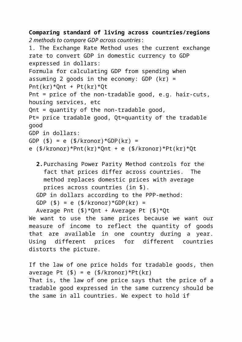
Comparing standard of living across countries/regions2 methods to compare GDP across countries: 1. The Exchange Rate Method uses the current exchange rate to convert GDP in domestic currency to GDP expressed in dollars:Formula for calculating GDP from spending when assuming 2 goods in the economy: GDP (kr) = Pnt(kr)*Qnt + Pt(kr)*Qt Pnt = price of the non-tradable good, e.g. hair-cuts, housing services, etc Qnt = quantity of the non-tradable good, Pt= price tradable good, Qt=quantity of the tradable goodGDP in dollars:GDP ($) = e ($/kronor)*GDP(kr) = e ($/kronor)*Pnt(kr)*Qnt + e ($/kronor)*Pt(kr)*Qt

2. Purchasing Power Parity Method controls for the fact that prices differ across countries. The method replaces domestic prices with average prices across countries (in $).

GDP in dollars according to the PPP-method:GDP ($) = e ($/kronor)*GDP(kr) = Average Pnt ($)*Qnt + Average Pt ($)*Qt

We want to use the same prices because we want our measure of income to reflect the quantity of goods that are available in one country during a year. Using different prices for different countries distorts the picture.

If the law of one price holds for tradable goods, thenaverage Pt ($) = e ($/kronor)*Pt(kr)That is, the law of one price says that the price of a tradable good expressed in the same currency should be the same in all countries. We expect to hold if transportation costs and differences in VAT are zero across countries. Assuming zero transportation costs and no country-differences in VAT, arbitrage tends to equalize prices across countries: It is profitable to buy the good where the price is low, and ship it to the country where the price is high. Higher demand in the country in which the price was initially low tends to put an upward pressure on the price in this country, and a higher supply in the country where the price was initially high tends to put a downward pressure on the price in this country. Thus, the market mechanism tends to equalize prices across countries for tradable goods.The law of one price does not hold for non-tradable goods and services:In a poor country, the price of a non-tradable good tends to be lower because of lower labor costs than in a richer country.Ex: e($/rupies)* Pnt(rupies) < Average Pnt($) PPP-adjusted GDP ($) for India > Not PPP-adjusted GDP ($) for India= GDP ($) according to the exchange rate method.Thus, the exchange rate method understates GDP ($) in poor countries.

Because domestic prices (in $) are lower in poor countries. In news reports you hear that in this country they earn 400 per capita and year. I have often thought: How can they survive? The explanation is that this income figure is not PPP-adjusted.

Purchasing Power Parity means that prices expressed in the same currency are the same across countries and regions. PPP does empirically not hold as prices on non-tradable goods tend to be lower in poor countries.

Application on Regions within a country: If nominal income per capita in the Stockholm region is twice as high as the nominal income per capita in the Karlstad region, the purchasing power of income per capita in the Stockholm region might be less than twice as high due to a higher price level; e.g. on non-tradable goods and services such as housing.

Measuring GDP through expenditures on final goods and services (method 1) in the real world in which countries have a public sector and do trade with other countries.Y is real GDP. P*Y= GDP in current prices.

Real GDP (Y) = C + I + G + NX (=Exports-imports)

C = real expenditures of households on final goods and services. Goods are sometimes categorized into nondurable and durable goods.

I = real expenditures on new machines, new buildings, and inventory build-up by firms. I is gross private investment.

G: real government spending on (/purchases of) final goods and services. Often (but not in the Mankiw textbook) G is split up into government consumption (GC) and government investment (GI).Examples of GC are expenditures on teachers’ and doctors’ salaries.Examples of GI is expenditures on new roads and government buildings.

Note: Government transfers to households such as unemployment benefits etc. are not included in G: Total government expenditures = G + government transfers to households (unemployments benefits, transfers to poor, to kids, to retired people) and to firms.

NX = real net exports = trade balance = value of exports of final goods and services – value of imports of final goods and services. Thus, NX is net expenditure from abroad on our goods and services.

Note: Capital stock this year = capital stock last year + I – depreciation (= reduction of the value of the capital stock). Net investment = I – depreciation.

One way to think about real variables. Assume that only one good is produced in the economy; e.g. corn. Then production, Y, is measured in tonnes of corn. Some of this corn is used for private consumption (C), some for private investment (it is planted in the ground to yield production next year) (I), some for government consumption and investment (G), and some of the production is shipped abroad (Export) and some corn is imported (Imports).(NX=exports-imports).Ex.: Y=C+I+G+NX: 100 = 50 + 20 + 20 + 10

Measuring GDP through income (method 2.).Other measures of income:Gross national product (GNP) = GDP – (wages and capital income of Swedish workers and firms operating abroad – wages and capital income of foreign workers and firms operating in Sweden).

By Swedish worker I mean a Swedish resident.

Gross National Product (GNP) = GDP + net factor income from abroad (NFI)In Swedish: Bruttonationalinkomsten till marknadspris (BNI) = Bruttonationalprodukten till marknadspris (BNP) + faktorinkomster från utlandet, netto (NFI).

GNP counts all final output produced by domestically owned inputs (workers and capital), no matter where those inputs are situated in the world.GDP counts all final output produced within the country regardless of who owns the inputs (foreign or domestic citizens) involved.

GNP is a income measure whereas GDP is a production measure.In a closed economy: GNP = GDPIn Stockholm: GDP > GNP as many workers compute to Stockholm but live in other regions e.g. Uppsala. That is, they contribute to GDP in Stockholm but their incomes are not part of the Stockholm GNP. GNP (Stockholm) = GDP (Stockholm) – wages of workers that live in other regions than Stockholm.

Another concept is disposable GNP (DGNP) DGNP = GNP + (transfers from foreign countries – transfers to foreign countries) = GNP + net transfers from abroad (NFTr).For Sweden: DGNP < GNP as net transfers from abroad are negative.

From now on we assume that net transfers from abroad = 0.In Swedish: Disponibel bruttonationalinkomst (DBNI) = bruttonationalprodukt till marknadspris (BNP) + faktorinkomster från utlandet, netto (NFI) + transfereringar från utlandet, netto (NFTr).

Other income measures:Net national product (NNP) = GNP – value of depreciation of capitalIn Swedish: Nettonationalinkomst till marknadspris (NNI) = Bruttonationalinkomst till marknadspris (BNI) – kapitalförslitning

National Income = NNP – Indirect taxes (such as the value added tax)In Swedish: Nettonationalinkomst till faktorpris = nettonationalinkomst till marknadspris (NNI) – indirekta skatterNational income = compensation to employees (70 %) + income to noncorporate business + corporate profits + net interest of firms.

Note: compensation to employees (workers) is total labor cost = gross income + social insurance contributions, which is around 2/3 of national income.

Personal Income = National Income- corporate profits - social insurance contributions - net interest received by the business sector + dividends+ government transfers to individuals + personal interest incomeIn Swedish: Hushållens inkomster

Disposable Personal Income = Personal Income – individual tax paymentsIn Swedish: Hushållens disponibla inkomst

Method 3 to calculate GDP implies:National income + indirect taxes + depreciation = GNP GNP – net factor income from abroad (NFI) = GDP

Simplifying assumptions in Classical and Keynesian model:NFI=depreciation of capital=indirect taxes=0Y =GDP=GNP=NNP= National Income = labor income (including taxes and social security contributions) + capital income

Assume: T = net taxes = tax payments – transfers to households.Households’ disposable income = Y - T

In Swedish:Y= BNP=BNI=NNI till marknadspris=NNI till faktorpris =Löneinkomster+direkta skatter + sociala avgifter + kapitalinkomster.

AGGREGATE SUPPLY: FACTOR MARKETS

Assume an aggregate production of Cobb-Douglas type:, where 0 < < 1.

Ex.: , easy to calculate with…

If there is one good in the economy, then Y is the quantity of this good.In kilograms, or liters depending on what the good is.

K = aggregate physical capital (machines and buildings)Should be measured by machine-hours and by hours buildings are used per year. But in reality K is measured by the real dollar value of the aggregate physical capital. It is then implicitly assumed that the real dollar value of K is proportional to the number of machine hours and hours buildings are used.L = aggregate labor input is measured by total hours worked (or by number of workers if every worker works the same number of hours). A = totalfactorproductivity, captures the effect on Y of all factors apart from K and L that impacts Y. For example, technological progress (innovations) or increased education of workers increases Y at given levels of K and L. Higher energy prices should decrease the use of energy and thereby also A and Y at given levels of K and L. Empirically is estimated to be around 1/3, which is the typical value of the share of capital income of national income.

The aggregate production function:Assume that K and A are constant: A=1, K=9, and =0.5. L Y/L

0 0 01 3 3 32 4.2 4.2-3=1.2 4.2/2=2.13 5.2 1 5.2/3=1.75 6.7 (6.7-5.2)/2=0.75 6.7/5=1.348 8.5 (8.5-6.7)/3=0.6 8.5/8=1.1From the table we see that:When L increases, Y increases but at a diminishing rate; because the capital-labor ratio decreases when L increases*MPL and APL(=Y/L) falls when L increases and K and A are constant.When MPL is below APL (=labor productivity), APL is decreasing.

Plotting the production function for A=1, K=9 and alpha = 0.5:

MPL is the slope of the production function.

If the stock of physical capital is higher: Parameters: A=1, K=16,

=0.5.A=1, K=16,

=0.5.A=1, K=16,

=0.5.L Y/L

0 01 4 4 42 5.6 1.6 5.6/2=2.83 6.9 1.3 6.9/3=2.35 8.9 1 8.9/5=1.88 11.3 0.8 11.3/8=1.4* MPL and APL increases when K (or A) increases and L is constant.This is shown by comparing the 2 tables above.

If A Y and MPL and APL at a given L (and K):Assume that A=1 and A=2 , K=9, and =0.5.

Summary:

MPL (= ) and Y/L decrease when L increases and K and A are constant.

MPL and Y/L increase when K (or A) increases and L is constant. By symmetry, the same holds for MPK and K:

MPK (= ) and Y/K decrease when K increases and L and A are constant.

MPK and APK(=Y/K) increase when L (or A) increases and K is constant.

Review of exponents

Definition: . E.g. and

Rule 1: Ex.:

Rule 2: Ex.:

Rule 3: Ex.:

Rule 4: Ex.:

Or more generally,

Production per worker, Y/L, increases if technology improves (A) or if every worker gets more capital (K/L)

Deriving the mathematical expression for MPL:

Review of the derivative: (1) If then

(2) If where b is a constant then

(3) More generally, then

Thus, MPL = (1-alpha)*(Y/L). That is, MPL is always lower than Y/L

2. exhibits constant returns to scale.If you e.g. increase each factor of production by 10 percent, then production also increases by 10 percent.If production increases by more, increasing returns to scale (IRS), and if production increases by less, decreasing returns to scale (DRS). CRS imply constant long-run average costs, IRS imply decreasing long-run average costs and DRS imply increasing long-run average costs when production increases.

The demand of K and L by firmsIn macro models households/individuals supply L and K (through saving as saving equals investment in a closed economy). Firms demand L and K.

Assumptions: There exist many identical firms that produce an identical good. Perfect competition is assumed The firms maximize profits.

The problem of the representative firm is to choose K and L and thereby output (Y) so that profits are maximized. Assuming two factors of production (K, L):

Profits ($) = Total revenue ($) – capital cost ($) – labor costs ($) Profits ($) = – –

where , P=price of the good, Y = quantity of the good, R= rental price of one unit of capital per period of time, W= nominal wage per worker per period of time.

Problem of the firm: Choose K and L (and thereby output) to maximize profits: Profits ($) = – –

Assuming perfect competition implies that the individual firm cannot influence prices: P, R and W are exogenous from the point of view of the firm. We also assume that A and are exogenous from the point of view of the firm as they are assumed to be given by the technology.

To maximize profits, the firm should choose K and L so that:

and

or and

Determining Equilibrium Factor Prices: They are found where Supply = DemandAssume that the supply of K and L is fixed: , Assume: , and A=1, = 0.5 , =9, =9:

Assume now that =16 due to labor immigration

Thus, If (due to labor immigration) and constant and W/P=MPL .

Domestic workers loose in terms of W/P from labor immigration, whereas domestic capital owners gain as . 2 other examples:(2) If (due to black death) and constant , W/P=MPL

Workers gain and capital owners loose income.(3) If and constant and W/P Workers gain and capital owners loose.

Conclusion: w/p and if

The distribution of income between workers and capital ownersAssume a closed economy, no taxes and no depreciation of capital:Real GDP = real capital income + real labor incomeIf assuming perfect competition:Real GDP (Y) = MPK*K+MPL*L.A unit of capital is paid its marginal product. A unit of labor is paid its marginal product.

Thus, the share of GDP that goes to capital owners is . The share of GDP that accrues to workers is 1- .You can go to the statistics and look up capital income as a share of national income to get an estimate of alpha. Typically, this estimate of alpha is about 1/3, both for developed and developing countries. Why?In poor countries: MPK is high and K is low and MPL is low and L is high.In rich countries: MPK is low and K is high and MPL is high and L is low.

Elaborating on the production functionA in the production function depends on business climate, tax levels, knowledge of workers, energy used, etc. If we particularly want to focus on energy used we might want to include this variable specifically in the production function:

, where 0 < , < 1 0<1- - <1.Knowledge of the work force measured by educational levelIn the basic formulation of the pf: , where 0 < < 1, an increase of the knowledge of the workforce e.g. measured by the educational level increases A. In an alternative formulation:

, where 0 < , < 1 0<1- - <1.Where H = number of workers with higher education, L = number of workers with low education. With this formulation of the production function, A does not capture the knowledge or the educational level of the work force.

GROWTH ACCOUNTINGMathematics: Proportional or percentage Changes in Economics.

Expressing levels into growth rates:

Rule 1. If y(t) = x(t)*z(t), then .

Ex.: Total Revenue (TR) = Price(P)*Quantity(Q) If P is raised by 10 % and sold quantity (Q) thereby decreases by 5%, then TR increases by 5 %.

Rule 2. If y(t) = x(t)/z(t), then .

Ex.: GNP per capita (y) = GNP(Y)/Population(Pop) If GNP (Y) increases by 5 % and the population increases by 3 % , then GNP per capita increases by 2 %.

Rule 3. If , then .

Rule 4. If ,

then

thus the growth rate of Y equals:(1) The growth rate of totalfactorproductivity.(2) The contribution of physical capital.(3) The contribution of labor.

Question addressed by so-called growth accounting (Mankiw, ch. 8, app.)growth accounting: How big share of the growth rate of the GDP can be attributed to changes in capital, to changes in the labor input and to changes in total factor productivity?

For developed countries we have good data on and ,

We have not direct data on as A captures the influence on Y of many

different factors on Y. E.g. taxes, climate for business, educational level of work force, infrastructure, social capital etc.Under perfect competion, , is the share of national income that is capital income, and (1- ) is the share of national income that is labor income. We have data on labor income and national income. Thereby, we get an estimate of .

Example:Year Y A K L2005 100 ? 300 10002006 103 ? 306 1010

and

0.03 = + 0.3*0.02 + 0.7*0.01

= 0.03 – 0.006 – 0.007 = 0.017.

0.017/0.03 = 0.57 : 57 percent of the growth rate of Y can be attributed to an increase in A. 0.006/0.03 = 0.2: 20 percent can be attributed to an increase in K.0.007/0.03 = 0.23: 23 procent can be attributed to an increase in L.

We have not explained why K, L and A changes over time.We have only been engaged in accounting.The neoclassical growth model explains why K and thereby Y increase. (A and L are exogenously given in this model; that is, they are determined outside the model.)

ECONOMIC GROWTHAim to explain why the standard of living (GDP/GNP per capita) changes over time. Main text: Mankiw, Ch. 7-8.Math: Growth rate = Percentage Change

, e.g. = 0.02, that is, 2 % .

where = income per capita year 0, = income per capita year 1. = growth rate/percentage change between year 0 and year1.

Analogously: ,

At a constant yearly percentage change (growth rate) income year 3 is:

where r = constant yearly growth rate/percentage change.

After t years and a constant growth rate income per capita equals: , where t = number of years.

Exercise: If GDP per capita (in 1995 prices) in 1995 and in 2000 was 194 and 222 thousands, what is the average annual growth rate during this 5-year period?

Graphical representation of the exponential function: . Let and r = 0.03:

If r increases, steeper slope. If y0 increases, the curve shifts upwards.

Students do not have to know logarithms:Alternative graphical representation of the function:

ln( ) = ln( ) ln( ) = ln( ) + ln( )

ln( ) = ln( ) +

This is the equation for a straight line: y = a + If r is a small number < 0.1

Formula: How many years does it take to double y at different growth rates?

ln(2) = ln( ) ln(2) = ln(2)/r t t ln(2)/r

If r = 0.05 t 14 years. If r = 0.015 t 46 years.

THE SOLOW GROWTH MODEL:Aim to explain the development over time of K and Y, k=K/L, and y=Y/L.

In the model the growth rate of the technological level, , and the growth rate of the numbers of workers, , are exogenous variables. In the model everyone is a worker. Thus, the number of workers = population.Thus, they are determined outside the model.

As , and are assumed to be exogenous variables, the model is about the accumulation of physical capital, and its effects on k, Y, and y.

To simplify we start by assuming: . Thus, the level of A and L are assumed to be constant over time.

Assumption (A1): The production function:, where 0 < < 1.

Expressing production in terms of per worker (labor productivity):

Labor productivity depends on:* Totalfaktorproductivity, A. If A Y/L * Physical capital per worker, K/L. If K/L Y/L

Note: (1- )* Labor productivity (Y/L) = MPL (= W/P)

Thus, the level of A and L are assumed to be constant over time.As L is assumed to be constant we can assume L=1. Small letters indicate that variables are expressed in terms of per worker.

In figure: A=1,2, and =0.5 .

Slope of the curve above is MPK=dY/dK.Note: L is assumed to be a constant; for example, L=1 K=k

More complicated proof which is optional:

[ , which is MPK:

MPK= ]

Assumption (A2): A constant share of income is saved (= a constant share of production is invested).

Goods market equilibrium condition: We assume a closed economy without a government sector: G=NX=0 S=Y-C=I National saving equals gross investment.

(A2): , where s is the share of income that is saved.

Note1: Y=GDP=GNPNote2: s is not saving per worker even though s is a small letter.

Moreover,

In figure: s=0.3, A=1, and =0.5. The vertical distance between the curves for production per worker, and investment per worker is consumption per worker. Assumption (A3): where is net investment, I = gross investment, and = depreciation of capital per period. is the depreciation rate, which is between 0 and 1; e.g. 0.05. (That is, 5 %). If , then If , then ; If , then .Expressing (A3) in terms of per worker:

Derivation optional:[

Using k = K/L , where =0 by assumption.

]

In figure:

The whole model:(A1): , the production function(A2): investment = saving (equilibrium condition) where saving is constant share of income.(A3): , The time path of the capital stock per worker

A-level students need not know mathematical derivation below:The whole model can be reduced to one equation:Inserting (A1) and (A2) into (A3):

The long-run equilibrium (steady state) value for k, , occurs when .That is, when gross investment equals depreciation

Solving for k in equilibrium:

What is the long-run equilibrium value of y, ?

If s or A and .

If the economy is not in its equilibrium, it converges over time towards the equilibrium because if k< , then i> , and if k> , then i< . See figure below.Showing the equilibrium in the Solow diagram:

In figure: A=1, s=0.3, , and =0.5.

The transition to equilibrium: a numerical exampleStarting below the equilibrium: The initial value of k: k(year=1)=4.00. Assume also: A=1, s=0.3, , and =0.5.year k

1 4.00 2.00 1.4 0.6 0.4 0.2 0.049 0.05 0.02452 4.2 2.049 1.435 0.615 0.420 0.195 0.047 0.046 0.02293 4.395 2.096 1.467 0.629 0.440 0.189 0.045 0.043 0.0214 4.584 2.141 1.499 0.642 0.458 0.184 0.043 0.040 0.0205 4.768 2.184 1.529 0.655 0.477 0.178…

9 3 2.1 0.9 0.9 0 0 0 0The equilibrium values of k and y are calculated by using the formulas:

,

How to fill out the Table based on an initial value and assumed parameter values: A=1, s=0.3, , and =0.5.Start by filling out the column for k based on the formula:

If k(year=1)=4, A=1, s=0.3, , and =0.5.

, , etc.After the values of k has been filled out, all other values of other variables (columns) can be calculated.

Graphical description of transition to equilibrium when economy start below and above the equilibrium ln( )=1.1:(1) k(t=1)=4, y (t=1)=2 , and ln(y (t=1)=2)=0.69 (2) k(t=1)=14, y (t=1)=3.74 , and ln(y (t=1)=2)=1.32

According to model:The growth rates of k and y are higher the lower k and y are. This explains why the slope of the curves for lny becomes flatter and flatter when lny approaches its equilibrium. Recall that the slope of lny is the growth rate of y. If two economies share the same equilibrium; that is, have the same parameter values on A, s (as well as on and ) but differ with respect to initial values, then the economy with lower k and y experience higher growth rates of k and y than the economy with higher k and y. the model says that y (and k) of these two economies converge over time. In other words, the model says that y over time converge across economies if the economies share the same equilibrium value of y).

Main lesson of empirical work on growth:Real per capita income tends over time to converge across economies, which are similar with respect to “institutions”.An economy with an initially relatively low real income per capita has on average a higher growth rate of real income per capita than an economy with an initially relatively high real income per capita if “institutions” are similar. Ex.: EU-countries and regions within countries.

Evidence from the OECD-countries (the currently rich countries)

Sample includes: Australia, Austria, Belgium, Canada, Denmark, Finland, France, Greece, Iceland, Ireland, Italy, Japan, Netherlands, New Zealand, Norway Portugal, Spain, Sweden, Switzerland, United Kingdom and USA.

Initially poor countries grow faster in terms of real GDP per capita during the period 1960-2000 than initially rich countries. The correlation between the average annual growth rate of real GDP per capita between 1960 and 2000 and real GDP per capita in 1960 = - 0.89

Evidence from the 24 Swedish Regions, 1911-1993

Regions that were relatively poor in terms of real income per capita in 1911, on average had a higher growth rate of real income per capita.

Higher growth rates in poor regions caused relative differences in real per capita income to diminish across the Swedish Regions between 1911 and 1993.

The dispersion is lower for real per capita income when it is adjusted for regional differences in cost of living as counties with high unadjusted real per capita incomes tend to have cost of living.

The empirical evidence on convergence in real per capita income across the Swedish regions is consistent with the predications of the textbook model:Low real per capita income

Little capital (physical + human) per worker,

Per capita Income adjusted and unadjusted for cost of living

Värmland moves to top category of per capita income when regional differences in cost of living are accounted for in 1993

Per capita income (p.c.i) is in 1980 prices

low wages, high rates of return to capital capital per worker production per worker income per capita Also factor mobility tends to contribute to convergence:Low wages and high returns to capital out-migration, and foreign investment capital per worker production per worker

Evidence from the countries of the world

Sample includes 80 countries.

No convergence in real GDP per capita across the countries of the world. The correlation between the average annual growth rate of real GDP per capita between 1960 and 2000 and real GDP per capita in 1960 = + 0.14.

Is lack of convergence in GDP per capita for the countries of the world, evidence against the model? NO!

The model says that if countries have the same equilibrium, the poorer country should grow faster in terms of y and k than the country that is richer in terms of y and k.

But if countries differ with respect to equilibrium, that is, with respect to values on A, s (as well as on and ), the poorer economy need, according to model, not grow faster than the initially richer economy.Africa is poor because it has a low equilibrium.Example that a rich country can grow faster than a poor country

Country A (Poor Country): A=1, s=0.2, , and =0.5 : ,Assumed initial values of k and y: 4 and 2. Country A’s growth rate of y=0

Country B (Rich Country): A=1, s=0.3, , and =0.5 : ,Assumed initial values of k and y: 5 and 2.24.

Country B’s growth rate of y is positive.

The short and long run effects of an increase of L (e.g. due to immigration)

A one-time increase of L:L(t=0)<L(t=1)= L(t=2)= L(t=3)= L(t=4) At time 1: K/L and Y/L, At time 2 and onwards: K/L and Y/L If the economy initially is in its equilibrium, it will over time revert to the initial equilibrium as gross investment exceeds depreciation of capital.

In figure: A=1, s=0.3, , and =0.5, K(0)=900, L(0)=100 and L(1)=200.The long run values of k and y are unchanged. However, adjustment takes a long time so migration plays a role for y during a long time according to model.What happens to the long run values of Y and K?

Size of economy increases when L increases.Example: increases from 3*100= 300 to 3*200=600, and increases from 9*100=900 to 9*200=1800.

In case of a pandemic, L decreases, the results are the opposite.

The effect of an increase in A

Old value: A=1, s=0.3, , and =0.5 and .New value: A=1.5 ,

The transition to the new long run equilibrium

Long-run growth of the number of workers

Before we assumed: L(0)=L(1)=L(2)=L(3)Now we assume : where n is the constant growth rate of the number of workers; e.g. 0.01.

Assumption A4. L(0)<L(1)<L(2)<L(3)

To keep k constant gross investment (I) now needs to compensate not only for depreciation of capital to keep k constant but also for the fact that the number of workers increases over time:(A3):

Derivation below optional:

[

Using k = K/L , where by assumption.

]

The whole model:(A1): , the production function(A2): investment = saving (equilibrium condition) where saving is constant share of income.(A3)+(A4): , The time path of the capital stock per worker

A-level students need not know mathematical derivation below:The whole model can be reduced to one equation:Inserting (A1) and (A2) into (A3)+(A4):

The long-run equilibrium

The long-run equilibrium (steady state) value for k, , occurs when .That is, when gross investment equals “depreciation”

Solving for k in equilibrium:

What is the long-run equilibrium value of y, ?

If n and .

The transition to the equilibriumIf the economy initially is in equilibrium and n the economy moves over time to the new lower equilibrium because when i< k:

In figure: A=1, s=0.3, , =0.5 and n=0 and 0.05.(1) when n=0 and .(2) when n=0.05 and .

The growth rates of aggregate variables:

In the steady-state:

Factor prices: In the model: C + I = Y = capital income + labor income = MPL*L+MPK*K= (W/P)*L + (r+ )Kr= real return on physical capital.Note: There is only one good in the Solow model, which is consumed or invested. If it is invested it is an asset which yields a return. K is the only asset in the economy. There exist no bonds, shares or money in the model.

Expressing the equilibrium condition above in terms of per worker: c + i=y=(W/P) + (r+ )k(1) W/P=MPL=(2) If k W/P and r In poor and rich countries K/L is low and high, respectively.If the value of A is the same in poor and rich countries, the real return on capital is higher in poor countries. As a result, we expect capital to move from rich to poor countries, increasing K/L in poor countries and lowering K/L in rich countries. Thereby, mobility of capital contributes to convergence in K/L between rich and poor economies. We expect L to move the opposite way because W/P is higher in rich countries. Mobility of L increases K/L in poor countries and decreases K/L in rich countries. Thereby, it also contributes to convergence in K/L between rich and poor countries.

Why do capital not flow to Africa? In other words, why are not large investments taking place in some African countries? Answer: Because A is low, which means that MPK=r+d is not so high.This can be seen in Solow-diagram. (Allow countries to differ w.r.t. A.)Important Exercise: Derive the equilibrium expressions for the real wage and for the real return on capital; that is, express the real wage and the real return to capital as functions of the exogenous variables: s, A, n, the depreciation rate and alfa.

Golden rule is optional reading for A- and B-level students:The golden rule level of capital:The level of capital that maximizes consumption per worker in equilibriumConsumption per worker is the distance between the curve for labor productivity ( ) and the curve for depreciation of capital per worker: (n+d)k. This distance is maximized at the level of k where the slopes of these two curves are

the same:

Solving the equation for k yields the answer.A government that wants to maximize consumption per worker should choose the saving rate (s) so that this level of capital is achieved.An economy can save too much. That is, by decreasing the saving rate per capita consumption can increase in the steady state.

Adding realism in the model: continuing technological progressThere is technological progress if new production techniques arise due to innovations such as the computer, engine, electricity, etc.

Model assumption: (A5): ,

[optional reading: ]where g =rate of technological progress is exogenously assumed.[Optional reading: The model is here formulated in continuous time which means that time changes continuously. Previously the model was in discrete time which means that the time is in periods. If the model were in discrete time:

.]

Only technological progress can explain long run increases in the living standard= GDP per capita = Y/L=y

Growth rates in the long-run equilibrium:

Before: , Now:

, , ,

Technological progress is exogenousAs the rate of technological progress is unexplained by the SOLOW model (that is, exogenous), adding g to the model does not add any more economic insights than the version of the model with g=0.For this reason and because it is simpler we will focus on the version of the model where g=0. Keep however in mind that technological progress makes the model more realistic because in the real world y typically increases over time due to new production techniques; that is, due to innovations.

What happens if the economy is off its equilibrium growth path?

When the economy approaches its equilibrium growth path, the growth rate of y deviates from the long-run growth rate (g). If an economy starts out below (above) the equilibrium growth path, the growth rate of y is higher (lower) than g. Holding constant the equilibrium growth path that is holding constant A(0), s, n, g, d and alfa, a lower y means a higher growth rate of y.

What happens to the growth rate and to the equilibrium growth path if the saving rate increases (or institutions improve or population growth )?

If s increases, the equilibrium shifts upwards, and the growth rate of y is higher than the long run growth rate during to the transition to the new equilibrium growth path.

A mathematical treatment:The Solow model with continuing technological progress:

Mathematical model (no need to understand details focus on figures). We do the model in continuous time instead of in discrete time:

(A1): ,

Where is a shift variable that increases if human capital of workers increases, if business climate improves, g is the rate of technological progress.

To get nice mathematical expressions we assume that technological progress is labor-augmenting which means that A is multiplied with L. (In case of a Cobb-Douglas pf labor-augmenting technological progress is equivalent to neutral technological progress that we thus far have assumed: Let Neutral technological progress.)

Model continued:We express all variables per effective worker, AL:(A1): where

(A2):

(A3):

Using

inserting (A4) and (A5):

In equilibrium:

,

Multiply both sides by A(t):

,

The equilibrium growth paths of k(t) and y(t).

In other words, the equilibrium is no longer a point but a time path.

These are the equilibrium growth paths of lnk(t) and lny(t):If the saving rate (s) increases, or the growth rate of the labor force (n) decreases ,or if increases due to e.g. a higher educational level among the workers, then the equilibrium growth paths of y and k shifts upwards. As the economy moves towards its new equilibrium growth path, the growth rate of y is higher than the long run growth rate (g).

Transition to the equilibrium growth pathIf the economy is not on its equilibrium growth path, it will over time move to its equilibrium growth path. Assume: A(0)=1, s=0.3, and (n+g+d)=0.1, g=0.015, n=0.015, d=0.07. =9, =3, ln( =3)=1.1We assume two different starting values:(1) =4, =2, ln( =2)=0.69, (2) =16, =4, ln( =4)=1.39To find out how K/AL develops over time, we use the transitional equation:

Multiplying with A(t) gives k(t), then it is trivial to find y(t) and lny(t):

When the economy approaches its equilibrium growth path, the growth rate of y deviates from the long-run growth rate (g). If an economy starts out below (above) the equilibrium growth path, the growth rate of y is higher (lower) than g. Holding constant the equilibrium growth path that is holding constant A(0), s, n, g, d and alfa, a lower y means a higher growth rate of y.

What happens to the growth rate and to the equilibrium growth path if the saving rate increases?Initially assume that the economy is on its equilibrium growth path and that: A(0)=1, s=0.3, and (n+g+d)=0.1, g=0.015, n=0.015, d=0.07. =9, =3, ln( =3)=1.1We assume that s increases to 0.4 =16, =4, ln( =3)=1.39

If s increases, the equilibrium shifts upwards, and the growth rate of y is higher than the long run growth rate during to the transition to the new equilibrium growth path.

Summing up the results:The long run growth rate of y is g; that is, the growth rate that occurs along the equilibrium growth path.

The growth rate of y = g + growth that occurs during the adjustment to equilibrium growth path.

Holding constant the variables that determine the equilibrium growth path constant; that is, A(0), s, and n, a lower y means a higher growth rate.

A(0) , s, or n

Increasing A(0), s or decreasing n shifts the equilibrium growth path upwards, and thereby induces transitional growth.

The growth rates of other variables in the model:

In the steady-state:

,

,

Testing the model empirically by regression analysis on a cross-section of countries:

where i = swe, Norway, finland, usa, etc.

According to model should be negative. And should be positive.

The dependent variable is typically the average annual growth rate of GDP per capita:

Alternatively an approximate formula,(it is approximate because in the real world data is discrete).

Note: gr for small r and g=ln(1+r)>r .

Other variables than the standard variables in the SOLOW modelIn empirical analysis often more variables than initial income per capita (or initial income per employed), the investment rate, the population growth rate are included. For example, educational level, variables measuring tax rates, corruption, openness to trade, population age structure, population density.

To make the empirical analysis fully consistent with the Solow model, it is typically assumed that these variables impact the level of technology (A) and thereby the steady state level of production per worker.Thus, A is assumed to depend on a host of variables.

If the model is tested in terms of per capita, often age structure variables; the share of the population below 15 and above 65 years, are included as explanatory variables in the regressions to account for the fact that people of these age groups typically do not work.

Factor mobility in the Solow model ((assume g=0).K will move from richer countries with low r (due to high k) to poorer countries where r is high due to low k. Thereby k and y will tend to equalize across countries. Nowadays, rich EU-countries invest capital or move production to new EU-countries or to CHINA or India.L will move the opposite way, from low-wage countries to high wage countries, which also contributes to equalize real wages, r and k across countries.Workers move from new EU-countries to old EU-countries where real wages are higher.

Specific example: assume two countries that are the same with respect to the parameters: A, n, d, and alfa, but one country has a higher saving rate than the other. Assume that these countries are in their respective equilibria.

Allowing for factor mobility across countries equalizes the real wage, the real return to capital, k and y across countries.The new equilibrium will be joint for the two countries and is determined by a weighted average of the saving rates in the 2 countries, where the weights are given by the size of the populations in the two countries.

Capital to labor (k) ratio is low in developing countries. As a result, one would expect a high real rate of return on investment in those countries. Why then do not a lot of investment (construction of new factories, etc.) take place in many of these countries? Answer: There is a lot of corruption, which makes the actual rate of return much lower; that is, after the investor have paid off a lot of government official, there might not be so much money left. A is low. There might also be a political risk. Investors might risk that some bandits take over the factories, like in Zimbabve.

Factors that impact GDP per capita in the real world:

POP = Population. If GDP per hour (=labor productivity) increases or the hours worked per employed increases or the number of employed as a share of population increases, then GDP per person increases.In other words, get each worker to produce more or get more people in production, then GDP per person increases.Production per employed (= the first 2 terms on the left hand side of the equation above) is in macromodels is GDP per worker, Y/L.

GDP (or GNP) per capita as a measure of the standard of living The income distributionGDP per capita (=average income) can be a poor indicator of the income of the average citizen; that is, of the median income.The median is the person in the middle of the income distribution.

The income distribution is typically assymmetric: median income < average income the more unequal income distribution the greater difference between median and average income and a larger proportion of the population tends to have an income below the average income. An extreme example:Country Equal. 10 individuals each with an income of 5000. The median and mean income is 5000. Country Unequal. 9 individuals each has an income of 2000.One individual has an income of 32000.Average income is 5000. Median income is 2000.GDP per capita as an indicator of “human development/happiness”We have concluded that average income per capita may be a poor indicator of the income of the average person; that is, of the median person.What is the relationship between income per capita and other indicators of “welfare/happiness”? We want (but cannot) measure is happiness/utility:U = U (y, x1, x2, x3, x4,…)Where y = income per capita, x1=literacy rate, x2=assess to clean water, x3= infant mortality rate, x4=life expectancy, etc.

2 views: 1. The correlation between income per capita and other variables (x1,x2,x3,x4,..) which we believe impact the welfare of people is high.

Therefore, it is sufficient to study determinants to income per capita.2.The correlation is not necessarily high.

The UN (UNDP’s) “Human Development Index” has 3 components:1. Life expectancy. 2. Educational level (e.g. literacy rate).2. Income per capita.

According to this index Sweden’s is a top 5 whereas with respect to income per capita Sweden is only top 20.

Problem of Household surveys that ask “Are you happy?” is that the meaning of the word happy may differ across cultures.We are rich now but are we happier?

The importance of relative position.Harvard-students were asked what alternative they preferred:

a) USD 50000/year whereas others get half.b) USD 100000/year whereas others get the double.

Source: The economist, Aug. 9, 2003.

Some characteristics of poor countriesLarge agricultural sector. They have a comparative advantage with respect to labor-intensive production as they have a lot of labor but only a little capital (physical and human).Demography: Young populations, many kids per woman.

ENDOGENOUS GROWTH MODELSEndogenous growth models rejects the assumption of the Solow model that technological progess is exogenous.

This equation shows what determines the growth rate of output Y/Y.Notice that as long as sA > , the economy’s income grows forever,even without the assumption of exogenous technological progress.

In the Solow model, saving leads to growth temporarily, but diminishingreturns to capital eventually force the economy to approach a steadystate in which growth depends only on exogenous technological progress.

By contrast, in this endogenous growth model, saving and investment canlead to persistent growth.

Start with a simple production function: Y = AK, where Y is output,K is the capital stock, and A is a constant measuring the amount ofoutput produced for each unit of capital (noticing this productionfunction does not have diminishing returns to capital). One extra unitof capital produces A extra units of output regardless of how muchcapital there is. This absence of diminishing returns to capital is the key difference between this endogenous growth model and theSolow model.

Let’s describe capital accumulation with an equation similar to thosewe’ve been using: K = sY - K. This equation states that the changein the capital stock (K) equals investment (sY) minus depreciation(K). We combine this equation with the production function, dosome rearranging, and we get: Y/Y = K/K = sA -

A second and more realistic class of endogenous growth models are complementary to the Solow model builds on Paul Romer (1990).

In the model above MPK does not fall when K increases. A second and more realistic class of endogenous growth models are complementary to the Solow model. They try to explain the long-run growth rate, g, which is exogenous in the Solow model, by the number of scientists, etc.

Read 2-sector model in Mankiw, ch. 8

THE LABOR MARKET (Mankiw: Ch. 6)Labor DemandThe firms are assumed to be price-takers in output and input markets; that is, P, W, and R are exogenous from the individual firms’ point of view. Assume also that the capital stock (K) is fixed; in other words, assume short-run analysis.A simple numerical example:If A=1, , , and

The profit-maximizing level of employment, , is given by:

Solving for as a function of the exogenous variables:

If e.g. W/P=0.75, then =4.

Note: A higher K increases the demand for L; Shifts the MPL-curve to the right.Graphical illustration of the numerical example:

In top figure: where is Y/L-curve? Where are profits?

LABOR SUPPLY, based on Varian section 9.8

Labor Supply: 3 possibilities:(1) Labor supply is unrelated to the real wage. (2) Labor supply increases when the real wage increases. (3) Labor supply decreases when the real wage increases: when the real wage

increases the individual can afford to take more leisure, which she likes. Factors that increase aggregate labor supply at a given real wage:1. Labor immigration. 2. Lower unemployment benefits should increase the labor supply of the domestic population.

The Microeconomics behind labor supplyThe individual or household faces the choice between consumption and leisure. More consumption requires more hours worked and hence less leisure.

The problem of the individual is to maximize:U = U(C,R)

where C= consumption during a period of time, e.g. a day.

R = hours of leisure enjoyed during a day.If C U(.), and if R U(.).

The two constraints the individual faces are:(1)The time constraint: where L = labor supply in hours,

is the time endowment which is 24 hours per day.(2) where P= Price of the consumption goodW = Nominal Hourly WageM= non-labor income, e.g. government transfers

Let In other words, is the quantity of goods that the individual receives that is not related to hours worked.

Now we have combined the two constraints that the individual faces, and the result is similar to the usual budget constraint: Thus, the goods that the individual derives utility from (C and R) are on the left-hand-side of the equation. And in front of the quantities of these goods are the respective prices of these goods W is the price of leisure: it is what the individual gives up by taking one hour of leisure. is called full or potential income. If R=0, then .

The constraint can be rewritten in real terms:

where 1 = real price of consumption, W/P is the real price of leisure = the quantity of goods the individual gives up by consuming one more unit of leisure.

Graphical illustration of the choice possibilities of the individual:

Let ,

Note: The choice constraint cuts the x-axis where R= .In the figure we assume that =1, and that W/P increases from 10 to 20.The numbers on the x-axis are 0.0, 0.1, 0.2,…, 1.0.Note also that labor supply (L) = - R: When R=0, then L= .

If W/P the intercept increases, and the slope becomes more negative.If W/P , the individual can afford more of both C and R. On the other hand, when W/P , R becomes more expensive in terms of the quantity of consumption goods the individual gives up by consuming one more unit (hour) of leisure.

3 hypothetical possibilities on demand for leisure and on labor supply (L= -R) when W/P :1.No effect on the demand for leisure and on the labor supply if the substitution (price) effect = income effect. The substitution effect is negative for the demand of leisure when the price of leisure (that is, the real wage) increases. The income effect for the demand of leisure is positive as a higher real wage means that the individual can afford and wants more leisure when income increases.2.Negative effect on the demand for leisure (= positive effect on labor supply) if the substitution effect > income effect.3. Positive effect on the demand for leisure (= negative effect on labor supply) if the substitution effect < income effect.

The optimal choice with positive non-labor income ( )

In the figure we assume that =1, W/P=10, and that increases from 5 to 10. The numbers on the x-axis are 0.0, 0.1, 0.2,…, 1.0.

When increases the individual wants more of both goods as they are assumed to be so-called normal goods. You want more of normal goods when your income increases.An increase of does not change the opportunity cost of enjoying leisure, and constitutes therefore a pure income effect.

Summary: The effect of changes in the exogenous variables on optimal demand for C and R, and on optimal labor supply:

If , , If W/P , ?, ?

A mathematical note on how to derive optimal demand-functions in case of a Cobb-Douglas (or a logarithmic) utility function:If the individual maximizes subject to the budget constraint: where x = quantity of good x, y= quantity of good y, = price of good x, = price of good y, and I= income.The optimal demand for x and y are such that the consumer chooses to spend a constant fraction of its income on these goods:

Note if ,

A mathematical example on the optimal choice of leisure (optimal labor supply):Assume that the individual has the following utility function: The constraints of the individual are: (1) (2) Note: W, P and can not be affected by the individual. Thus, they are exogenous from the point of view of the individual.

Combining the constraints yields:

The result is similar to the usual budget constraint: Optimal demands for C and R, and optimal labor supply are:

When :If , , If W/P , , : More labor is supplied when W/P .When :If W/P , =0.5 and =0.5. That is, labor supply and optimal leisure are unrelated to W/P.Thus, the substitution effect equals the income effect.

CONSUMPTIONAccording to Keynesian theory the private consumption function is:

, Where T=net taxes=taxes – transfersY-T=disposable income Current private consumption depends on current disposable income.More elaborate theories say that current consumption depends not also on expected future disposable income, Wealth, and on the interest rate. For example, we expect an increase in wealth to increase current consumption at a given level of Y-T, which would increase in the equation above.

A Simple Model of Intertemporal Choice over the life-cycle.Assumptions: The individual lives 2 periods.The individual consumes in both periods and also receives incomes in both periods. The incomes are exogenously given.We assume a perfect capital market, which means that the individual can borrow and lend as much as she wants at a given interest rate.The individual receives and leaves no bequest.

Preferences are represented by the utility function: U(C1,C2)where C1=consumption in first period of life, and C2=consumption in second and last period of life. The individual values both goods (C1 and C2). The marginal utility of C1 is diminishing when C1 increases (and C2 is constant), and the marginal utility of C2 is diminishing when C2 increases (and C1 is constant).Diminishing marginal utilities implies that the individual wants to “smooth” consumption rather than consuming a lot in one period and little in the other period. The perfect capital market, which implies that the individual can lend and borrow at a given interest rate, makes consumption “smoothing” possible. A consequence of diminishing marginal utilities is that if income only is received in one period of life, the individual wants to spread this income over both periods of life. If income increases only in one period, the individual wants to spread this increase of income over both periods.

The constraints: (1) S=Y1-C1, (2) C2=(1+r)S+Y2where S = Saving in first period of life (can be negative), r=interest rate, Y1 and Y2 income net of taxes received in period 1 and in period 2.Combining the constraints (1) and (2): C2=(1+r)*(Y1-C1) + Y2The budget constraint in figure above:

Slope of the constraint:

Giving up one unit of C1 means more than one unit of C2 can be consumed because of positive return (interest) on saving. Thus, C1 is “more expensive” than C2.

The budget constraint can also be written:

Present value of life-time consumption = Present value of life-time incomeWhat is a present value? If r=0.05, the present value, x(t), of a value next year, x(t+1): e.g. 105 dollars, is the value you have to deposit in a bank today to receive 105 dollars next year. Thus, x(t)*(1+r)=x(t+1). If there is no uncertainty, and there is a perfect capital market, the individual should be indifferent between receiving 100 dollars today and receiving 105 dollars next year if the interest rate is 5 %.

Here are the combinations of first-period and second-period consumptionthe consumer can choose. If he chooses a point between A and B, he consumes less than his income in the first period and saves the rest for the second period. If he chooses between A and C, he consumes more thathis income in the first period and borrows to make up the difference.

First-period consumption

Seco

nd-

perio

dco

nsu m

ptio

n Consumer’s budget constraintConsumer’s budget constraint

Saving

BorrowingA

C

B

Horizontal intercept isY1 + Y2/(1+r)

Horizontal intercept isY1 + Y2/(1+r)

Vertical intercept is(1+r)Y1 + Y2

Vertical intercept is(1+r)Y1 + Y2

Y1

Y2

The intertemporal budget constraint above corresponds to our usual budget constraint that has prices in front of the quantities:

where P1= price of current consumption=1, P2=1/(1+r)=the price of future consumption. P1>P2. Because if giving up one unit of C1, positive interest on savings means more than one unit of C2 can be consumed. Thus, C1 is more expensive than C2.

If either Y1 or Y2 , the budget constraint shifts outwards.

and because of diminishing marginal utilities. The optimal levels

of C1 and C2 depends on the present value of life-time income, :

and

Regardless of whether Y1 or Y2 increase, the consumer spread the increase

in over both periods.

If Y1 ,as the consumer wants to increase consumption in both periods.If Y2 , for the same reason. Thus, if Y2 . This result does not happen in the Keynesian model.

If the interest rate increases, C1 becomes more expensive relative to C2.The substitution effect is that you consume less of the good whose price has increased, , and more of the other good, .

For a saver: If r , a saver becomes richer: the income effect: and .The net effect (substitution + income effect): , ? , S=(Y1- )?

For a borrower:If r , a borrower becomes poorer: the income effect: and .The net effect (substitution + income effect): , S=(Y1- ), ?In aggregate an economy typically saves: r S=(Y1- )?It is often assumed that an increase in r has no or a positive effect on S.

Borrowing constraints: C1 Y1Consider an individual that consumes less than she would like in period 1:If Y1 , . That is, she uses all of the increase in Y1 for C1.

Borrowing constraints are facts of life: They should increase aggregate saving in the economy, but may be an obstacle for small-business that may have profitable investment projects that the banks might not want to lend money to because of imperfect information.

Economists decompose the impact of an increase in the real interestrate on consumption into two effects: an income effect and asubstitution effect. The income effect is the change in consumptionthat results from the movement to a higher indifference curve. Thesubstitution effect is the change in consumption that results from thechange in the relative price of consumption in the two periods.

Economists decompose the impact of an increase in the real interestrate on consumption into two effects: an income effect and asubstitution effect. The income effect is the change in consumptionthat results from the movement to a higher indifference curve. Thesubstitution effect is the change in consumption that results from thechange in the relative price of consumption in the two periods.

First-period consumption

Seco

nd-

perio

dco

nsum

p tio

n

B

IC1IC2

AC

An increase in the interest rate rotates the budget constraint around the point C, where C is (Y1, Y2). The higher interest rate reduces first period consumption (move to point A) and raises second-period consumption (move to point B).

An increase in the interest rate rotates the budget constraint around the point C, where C is (Y1, Y2). The higher interest rate reduces first period consumption (move to point A) and raises second-period consumption (move to point B).

New budgetconstraint

Old budget constraint

Y1

Y2

The motive for saving in the intertemporal choice model is that the individual wants to smooth consumption over the life-time. If we add uncertainty to the model, people also save because future income may be uncertain or because the individual might live longer than expected. This is called precautionary saving.

Modigliani’s life-cycle model, and Friedman’s permanent income hypothesis builds on the microeconomic intertemporal choice model above.

Mathematical Example with a common utility functionThe individual/household chooses C1 (and thereby S and C2) to maximize

, where

If the individual is impatient which is a common assumption: The budget constraint of the individual is:

where r, Y1 and Y2 cannot be affected by the individual (are exogenous).

Note: The solution to the mathematical problem is such that the endogenous (the choice) variables are expressed as functions of the exogenous variables.

If , ; if Y1, if Y2.

If r , ,

Borrowing constraints: C1 Y1Consider an individual that consumes less than she would like in period 1:If Y1 , . That is, she uses all of the increase in Y1 for C1.

Borrowing constraints are facts of life: They should increase aggregate saving in the economy, but may be an obstacle for small-business that may have profitable investment projects that the banks might not want to lend money to because of imperfect information.The motive for saving in the intertemporal choice model is that the individual wants to smooth consumption over the life-time. If we add uncertainty to the model, people also save because future income may be uncertain or because the individual might live longer than expected. This is called precautionary saving.

Modigliani’s life-cycle model, and Friedman’s permanent income hypothesis builds on the microeconomic intertemporal choice model above.

EXERCISE:

Combining the intertemporal choice model with endogenous labor supply

Assume that Y1 and Y2 are not exogenous from the point of view of the individual. Assume that Y1=W1*L1, where L1=1-R1, where L1 is hours worked in period 1, and R1 is hours of leisure in period 1. 1=L1+R1 equals time endowment (total number of hours available) in period 1 that is normalized to 1. Assume also that Y2=W2*L2, where L2=1-R2, where L2 is hours worked in period 2, and R2 is hours of leisure in period 2 of life. 1=L2+R2 equals total number of hours available in period 2 that are normalized to 1. We also assume that W1 and W2 are exogenous from the point of view of the individual. Assume: Where the preference parameters, , all are assumed to be between zero and 1.Write up the intertemporal budget constraint of the individual. Derive the optimal levels of C1, C2, R1, R2, L1, and L2 as functions of the exogenous variables.What happens to the optimal levels of C1, C2, R1,R2, L1, and L2 if W2 increases?

GOVERNMENT DEBT When a government spends more than it collects in taxes, it borrows from the private sector to finance the budget deficit:

Size of government debt

To compare the government debt across countries or over time it should be related to income; that is, to GDP or to GNP.When does Debt/GDP increase?

•Real business cycle theory emphasizes the idea that the quantity of labor supplied at any given time depends on the incentives that workers face. •The willingness to reallocate hours of work over time is called the intertemporal substitution of labor.Consider this example:Let W1 be the real wage in the first period. Let W2 be the real wage in the second period.Let r be the real interest rate.If you work in the first period, and save your earnings, you will have(1 + r)W1 a year later. If you work in period 2, you will have W2.

If G-T =0, Debt/GDP increases if the r > growth rate of GDP

Problems in measurement:1.Debt should be measured in real terms2. Government not only has a debt but also assets. The budget procedure that accounts for assets as well as liabilities is called capital budgeting. Under capital budgeting, government borrowing to finance the purchase of a capital good would not raise the deficit.3. The government budgets deficit is countercyclical. It increases in a recession and decreases in a boom. To see whether fiscal policies are expansionary economists often calculate a cyclically-adjusted budget deficit: the government budget deficit at the full-employment output.

The intertemporal budget constraint of the government:

This intertemporal budget constraint implies that the present discounted value of net taxes must cover the present discounted value of government spending plus the initial government debt.

Lower taxes today means higher taxes in the future.Thus, an increased tax burden on future generations.

Do government budget deficits imply a tax burden on future generations?The intertemporal budget constraint of the government shows that the government can redistribute across generations. It shows e.g. that if the government lowers T1,which benefits the current generation, the government must raise future taxes, which hurts “the future generations”. Also spending :G1, G2, benefits different generations.

The Ricardian view on whether a tax cut can stimulate the economy:

A tax cut today will mean higher future taxes for the households so that their present value of life-time income will be unchanged, so private consumption is unchanged. Households only increase their saving in response to a tax cut today. Thus, no effect on Y.

Also an increase in G will have a lower effect on Y as people realize that a higher G will imply higher taxes in the future, so households’ life-time income will go down so households will cut their consumption and increase their saving. Thus, lower effect on Y of an increase of G as people at the same time cut their consumption. Y=C+I+G.

Proponents of the Ricardian view assume that people are rational when making decisions such as choosing how much of their income to consume and how much to save. When the government borrows to pay for current spending, rational consumers look ahead to anticipate the future taxes required to support this debt.

Why the ricardian view might not hold? That is, why a tax cut today may increase current consumption even though future taxes must be higher, leaving the life-time income in present value of the consumers unchanged.1. Short-sighted consumers. 2. Borrowing constraints: The theory says that people want a smooth consumption over time to diminishing marginal utility of consumption at a particular point of time. The Ricardian view is that consumers base their spending not only on current but on their lifetime income, which includes both current and expected future income. Advocates of the traditional view of government debt argue that current consumption is more important than lifetime income for those consumers who face borrowing constraints, which are limits on how much an individual can borrow from financial institutions.

A person who wants to consume more than his current income must borrow, for example because his current disposable income is low, e.g. for students. If he can’t borrow to finance his current consumption, his current income determines what he can consume, regardless of his future income. In this case, a debt-financed tax cut raises current income and thus consumption, even though future income is lower. 3. Also generations may not be altruistic towards their kids so they do not compensate their kids with a higher bequests to compensate for higher future taxes.

The Laffer-curve: Tax rates and total tax revenues:Government tax revenues=Tax rate*Y(L(tax rate))If the tax rate increases tax revenues increases ceteris paribus.However, higher taxes might lower labor supply and thereby production.Laffer pointed out that government revenues actually can actually fall when tax rates are increased.

Government bonds that are indexed with inflation:The return is based on CPI, and when the principal (the price of the bond when it is issued) is repaid by government it is increased by rate of inflation.The interest rate paid on the bonds, therefore, is a real interest rate. Indexed bonds reduce the government’s incentive to produce surprise inflation to reduce the real value of its debt.

2-period model to show the Ricardian view:Assumptions:

(1)if G>T, the government borrows from the public.

(2)The government is assumed to “live” 2 periods and balance its budget over these 2 periods.Combining equations (1) and (2):

Present value of income equals present value of consumption.

The consumer maximizes by choosing C1, (and thereby S and C2) subject to the constraints: (1) S=Y1-T1-C1, (2) C2=(1+r)S+Y2-T2where S = Saving in first period of life (can be negative), r=interest rate, Y1-T1 and Y2-T2 net income received in period 1 and in period 2.Combining the constraints (1) and (2):

C2=(1+r)*(Y1-T2-C1) + Y2-T2

If the government decreases T1 to stimulate aggregate demand it must increase T2 due to the government’s intertemporal budget constraint:

because G1 and G2 are assumed to be constant.

How is private consumption (C1) impacted by the decrease of T1?The present value of the life-time income of the consumer is not affected by T1. As a result, C1 is unchanged, and Y1 is unchanged.

What is the effect on private saving of T1?

Private saving increases when T1

What is the effect on public saving? When current net taxes are lowered, public saving decreases.

There is no effect on aggregate saving, the decrease of public saving is fully compensated by an increase in private saving.

As aggregate saving is unchanged, the interest rate is unchanged, and the domestic investment is unchanged. Also C1 and C2 are unchangedwhich means that aggregate demand is not impacted.

THE FERTILITY CHOICEAssume that a household derives utility from a consumption good and from having kids. Assume the following utility function:

where C is quantity of consumption goods and K is number of kids. (You may use the greek notation for alfa.)Alfa is assumed to have a positive value.

Assume that W is the wage income that the household receives if the household works full time. Note that if y=lnx, then dy/dx=1/x(Assume also that the household lack other sources of income than labor income.) Assume that the price of the consumption good is 1.Assume that the price of (the cost of) children is related to the wage income. This is the case because when the household have kids, it is assumed that the household no longer can work full time because the have to look after/raise the kids. Thus, the household give up part of the wage income, which constitutes the price (cost) of kids. Assume that the price per kid is W*beta, where beta is the proportion of the household’s full time that the each kid require. For example, if beta=0.2 and the household has one kid, then 80 percent of the time of the household is devoted to work and 20 percent is devoted to the kid. If the household has 2 kids, 60 percent of the time is devoted to work and 40 percent is devoted to raising these two kids.a.Write up the budget restriction of the household. 2pb. Derive the optimal levels of C and K as functions of the exogenous variables. 4pAssume that the wage income is exogenous from the point of view of the household.Also show the optimal choice graphically with C on the vertical axis and K on the horizontal axis. c.What happens to the optimal choice of C and K if W increases. Show mathematically by using the derivative.What happens to the utility level of the household. Explain why! 2pd. Is this theoretical effect consistent with empirical observations from the real world? 1pe. What happens to the optimal choice of C and K if beta increases? Show mathematically. What happens to the utility level of the household. Explain why. 1p