Weather, mood, and voting:An experimental analysis of the effect of weather beyond

turnout

Anna Bassi∗†

————————————————————————————————————–

Abstract

Theoretical and empirical studies show that inclement weather on an electionday reduces turnout, potentially swinging the results of the election. Psychologystudies, however, show that weather affects individual mood, which – in turn –affects individual decision-making activity potentially beyond the simple decisionto turn out on an election day. This paper evaluates the effect of weather, throughits effect on mood, on the way in which voters who do turn out decide to casttheir votes. The paper provides experimental evidence of the effect of weather onvoting when candidates are perceived as being more or less risky. Findings showthat, after controlling for policy preferences, partisanship, and other backgroundvariables, bad weather depresses individual mood and risk tolerance, i.e.. votersare more likely to vote for the candidate who is perceived to be less risky. Thiseffect is present whether meteorological conditions are measured with objectiveor subjective measures. This draft: May 20, 2013.Word-count: 8467

————————————————————————————————————–∗The University of North Carolina at Chapel Hill, Department of Political Science†An earlier version of this paper has previously circulated as “The indian rain dance of the incum-

bent. The effect of weather beyond turnout.” I am grateful to Daniel Butler, David Cesarini, StanleyFeldman, Andrew Healy, Luke Keele, Neil Malhotra, Michael MacKuen, and Agnieszka Tymula forhelpful comments. I would like to thank the Behavioral Lab at UNC Kenan-Flagler for providing partof the financial support for this paper, and seminar’s participants at the 2012 Midwest Political ScienceAssociation, 2013 Southern Political Science Association, and 6th Annual NYU-CESS ExperimentalPolitical Science Conference for providing valuable feedback. All errors remain my own.

1

Much has been written about the effect of bad weather on Presidential Election Day

turnout and whether it benefits one party over another. The issue of weather and its

impact on elections is one that receives constant media and political campaigner hype

at every election. Understanding the possible effects of weather conditions on voting

behavior is crucial: in today’s contentious elections, even a small difference in num-

bers of votes over a large geographical area could tilt the vote one way or the other.

For example, Ludlum (1984) finds that weather proved decisive in the presidential

election of 1960, when John F. Kennedy defeated Richard Nixon by a razor-sharp

margin of 11,500 votes in five states. Heavy rains, caused by a cold front in swing

states like Illinois, deterred rural voters (mostly Republicans) from going to the polls,

while not affecting the urban voters (mostly Democrats) in Chicago. The analysis of

other cases (Ludlum, 1984) confirm this effect, providing support for an axiom of New

York politics that holds that [...a rainy day favors a Democratic candidate since the

upstate Republicans would not turn out in full in inclement weather, while the urban

Democrats would not be put to undue inconvenience.] (Ludlum, 1984, p. 102)

With Republicans continuing to hold a greater share of the vote in rural areas and

Democrats continuing to dominate in urban areas, the New York politics’ adage seems

not to hold anymore. Recent studies (De Nardo, 1980; Knack, 1994; Gatrell and

Bierly, 2002; Gomez et al, 2007, Keele and Morgan, 2013) show mixed results.

Although the issue of weather and its effects on elections is one that invariably arises

in every election year, most of the literature focuses on the effect of weather on

turnout exclusively: these studies fail to investigate whether the effect of weather

goes beyond turnout, affecting the way in which voters, who do turn out, decide how

to cast their vote. However, some findings (Gomez et al., 2007) suggest that the ef-

fect of weather on parties’ vote share may be greater than the indirect effect through

turnout (their findings show that for every inch of rain above average, turnout de-

creases only by approximately 0.9%, but that the Republican candidate receives ap-

proximately an extra 2.5% of the votes). Few studies have investigated this question.

The effect of extreme weather (such as natural disasters) has been analyzed in a con-

text of public opinion and elections by Healy and Malhotra (2010), who analyze the

effect of tornados on electoral outcomes, finding that voters appear to reward or pun-

ish the incumbents according to their perceived performance in handling the disaster.

Gerber (2013) studies the relationship between partisanship and climate policy of the

local government. Cohen (2011) tackles the question of how general weather affects

public opinion, finding a positive relation between presidential approval ratings and

sunshine exposure.

To have a better understanding of the effect of weather on voters’ decisions, we need

to both assess the effect of weather on voters’ actions and beliefs and to understand

the mechanism through which climate conditions exert such an effect. Psychology

literature suggests that weather affects both conscious and subconscious mood and

that mood affects human behavior. Whether, however, the effect of weather on mood

is strong enough to drive human’s behavior is less clear.

Laboratory experiments provide the best tool for testing these behavioral questions

because of the precise control that they afford and the possibility to analyze data

that do not naturally occur (Woon, 2012b). Bassi et al. (2013) provides experimen-

tal evidence of the link between weather, mood, and risk aversion. Similarly, this

paper investigates whether such an effect is present in a voting setting. Specifically,

this paper identifies the existence of an effect of weather on individual voting deci-

sions. Findings suggest that sunlight and good weather have a positive impact on

the likelihood of voting for riskier candidates, while voters rely more heavily on less

risky candidates in bad weather. This result holds for both objective and subjective

measures of weather conditions.

2

Furthermore, this paper helps identify a specific pathway through which weather af-

fects voting decisions. The paper provides an analysis of the mechanism at work by

employing a psychological questionnaire called PANAS-X (Watson and Clark, 1994)

used to measure respondents’ moods. I find that “positive mood” feelings such as

self-assurance and attentiveness display a statistically significant decrease in bad

weather conditions, while sadness displays a statistically significant increase. Re-

sults also show that positive mood feelings and states that are sensible to weather

conditions are also positively associated with the likelihood of voting for a riskier

candidate. I interpret these findings as offering evidence of a causal mechanism at

work: the impact of weather (through mood) on voting choice. Subjects are more will-

ing to accept the level of risk associated with a risky candidate when they are in a

better mood.

1 Weather, Mood, and Behavior

The impact of sunlight and weather in general on human mood has been widely exam-

ined in the clinical psychology literature. For example, good mood has been associated

with low levels of humidity (Sanders and Brizzolara, 1982); high levels of sunlight

(Cunnigham, 1979; Parrot and Sabini, 1990; and Schwartz and Clore, 1983); high

barometric pressure (Goldstein, 1972); and high temperature (Cunningham, 1979;

Howarth and Hoffman, 1984). Furthermore, the effect of temperature and sunlight

is especially strong in the spring, when people have been deprived of such weather

(Keller et al., 2005).

By the same token, mood has been proven to significantly affect how individuals make

decisions. For example, research in experimental psychology has proven that mood

affects the way agents make decisions in risky or uncertain environments by affecting

their levels of risk aversion. A person’s mood may affect the subjective judgment of the

3

likelihood of a future event (Wright and Bower, 1992): a happy person is “optimistic,”

i.e., she reports higher probabilities for positive events and lower probabilities for

negative events. Conversely, a sad person is “pessimistic,” perceiving lower (higher)

probabilities to be attached with positive (negative) events. Experimental studies

have documented a negative link between anxiety (and depression) and “sensation

seeking” measures, which have been extensively documented to be reliable proxies

for risk-taking behavior. More recently, Eisenberg et al. (1998) show in experimental

studies that depressed individuals tend also to be more risk averse in a series of hy-

pothetical everyday-life situations. In this framework, people in a good mood would

be more willing to engage in activities and choices yielding a degree of risk. This con-

duct has been identified in the literature as “mood-risk tolerance” channel. Bassi et

al. (2013) show that weather affects risk aversion through this “mood-risk channel.”

Mood on Election Day can swing voter choice of a marginal voter – the one who is still

undecided – through this “mood-risk tolerance” channel. A voter who is virtually or

almost indifferent between two candidates might lean toward the “riskier” candidate

when she feels in an upbeat mood, or might resort to the “safer” candidate when she

feels more depressed or pessimistic. If the “safer” choice is also equivalent to the

status quo, this effect can also be interpreted as “status quo bias,” “loss aversion,”

“endowment effect,” or “regret avoidance.”

A related stream of literature analyzes the effect of emotions on risk assessments.

Johnson and Tversky (1983) show a positive link between emotions and risk assess-

ments, indicating that optimistic emotions lead to optimist risk assessments and vice

versa. Hsee and Weber (1997) suggest that positive emotions lead to greater risk

seeking because people are more optimistic about future outcomes, while negative

emotions such as anxiety make agents more pessimistic about the future and thus

more risk-averse. What makes the literature on mood and emotions complementary

but not equivalent is the fact that, although mood and emotions are tightly linked,

not all negative emotions lead to negative mood states and viceversa (DeSteno et al.,

4

2000). Druckman and McDermott (2008) show that emotions need to be differenti-

ated beyond their positive or negative general state, as different negative emotions

exert opposite effects on individuals’ risk attitudes. MacKuen et al. (2010), Huddy et

al. (2007), and Feldman et al. (2013) stress that negative emotions such as anxiety

need to be distinguished from other negative emotional responses such as anger.

This paper explores the way in which weather influences how individuals vote be-

tween candidates framed as risky choices via a “mood-risk tolerance” channel. Mood

may provide an important key in explaining the different effects of weather variables

on voting behavior. The goal of this paper is to enrich, rather than negate, earlier

findings on the effect of emotions on elections and public opinion by analyzing how

the mood variables that are susceptible to change with weather conditions affect vot-

ing. I next describe how individuals’ risk assessments map into voting decisions. A

similar approach has been taken by Eckel, El-Gamal, and Wilson (2009), who investi-

gate the link between risk preferences and emotions in a sample of hurricane Katrina

evacuees right after the natural disaster and a year later, finding the first sample to

be more risk-loving than the second. The authors ascribe the higher risk tolerance of

the first sample to the prominence of negative emotions.

2 Uncertainty, Prospects, and Risk Attitudes

As Berinsky and Lewis (2007) suggest, analyzing the question of whether risk at-

titudes affect voters’ preferences regarding risky candidates requires discussion of

the (1) specification of the voters’ utility function over different candidates; and (2)

specification of how the uncertainty about future outcomes enters in their utility cal-

culations.

Concerning the first question, the standard approach – the expected utility model –

assumes that the individual utility function is concave, that is, the marginal utility

5

of an additional dollar diminishes when the total utility increases (Bernulli, 1954).

However, Kahneman and Tversky (1979) argue that individuals display diminishing

marginal utilities only for prospects with positive outcomes, while displaying increas-

ing marginal utilities for prospects with negative outcomes, suggesting that individ-

uals are risk-averse for gains, but risk-seekers for losses. The key element of this

argument is that individuals engage in decision making first by identifying a ref-

erence point from which people tend to be risk-averse for gains and risk-loving for

losses. Therefore, risk aversion is a function not only of the riskiness of an option, but

also of its desirability (see McDermott, 2001, for a comprehensive review).

The way in which individuals interpret their choices, as gains or as losses, influences

how much risk they will take. As has been found in several experiments on framing

(Druckman, 2001a, 2001b, 2001c), the way in which information is framed influences

individuals’ judgment as well, in that it affects how they interpret their choices. Kah-

neman and Tversky (1979) found that framing a policy as a gain (for example, by

describing a 10% rate of unemployment as an employment rate of 90%) induces indi-

viduals to consider their choices in a domain of gain, while framing the same policy

as a loss induces them to consider their choices in a domain of losses.

As regards the second question, Alvarez and Franklin (1994) suggest that no consen-

sus exists in the literature on how uncertainty affects the voter’s evaluation of the

candidates. Most of the literature focuses on the uncertainty about the policies that

the candidates would put in place once elected: Shepsle (1972), Enelow and Hinich

(1981), Bartels (1998) and Palfrey and Poole (1987). consider how the uncertainty

about candidate locations enters voters’ expected utility. Alternatively, Quattrone

and Tversky (1988) focus on how uncertainty about candidates’ performance affects

voting choice. They test a voting choice between an incumbent and a challenger with

identical policy preferences but with different degrees of likelihood to implement the

policy. Quattrone and Tversky (1988) confirm Kahneman and Tversky (1979)’s pre-

dictions in a social choice domain: voters are averse to voting for risky candidates

6

in the domain of gains but they do seek out the riskier candidate in the domain of

losses. This prediction has been extended to data from real-world elections in Mex-

ico by Morgenstern and Zechmeister (2001), who found risk attitudes to be a strong

determinant of voter behavior when deciding between an incumbent and a challenger.

As the objective of the paper is to analyze the way in which weather influences voting

decisions via a “mood-risk tolerance” channel, the paper’s design builds on the Quat-

trone and Tversky (1988) classical design, in which respondents vote between two

candidates with identical policy preferences. This assumption, though not natural in

all situations, provides a necessary preliminary to a more general analysis and may

be reasonable in some circumstances (for instance in parties’ primaries, in which

policy differences might be negligible). With this design, the impact of background

personal characteristics on individual decision-making in voting choices is controlled

for, and the effect of weather on individual choices can be imputed to its effect on the

individual level of risk aversion caused by mood.

3 Expectations and Conjectures

The expectations about the experimental results can be described by the following

hypotheses.

1. The vote share for a risk-free candidate is larger than the vote share for a risky

candidate who yields the same expected utility in a positive prospect.

I expect this finding, because according to both the standard expected utility

theory and prospect theory, agents are risk-averse in the positive domain. So,

when an individual is presented with two candidates who are identical in all

dimensions but for the degree of risk that they yield, individuals are expected to

choose the one candidate who carries the least risk.

2. The vote share for a risk-free candidate is larger in the domain of gains (positive

7

prospect) than in the domain of losses (negative prospect).

According to prospect theory, agents are more risk-averse in the positive domain.

So, voters are expected to choose the one candidate who carries the least risk

more frequently in the positive prospect than in the negative one.

3. The vote share for a risk-free candidate is smaller than the vote share for a risky

candidate who yields the same expected utility in a negative prospect.

According to prospect theory, agents are not only more risk-tolerant in the nega-

tive domain, but they actually seek risk. Voters are therefore expected to choose

the one candidate who carries the most risk, but who can yield a positive or

higher outcome.

4. The vote share for a risk-free candidate is larger in bad weather days than in

good weather days.

Regardless of the prospect framing, I expect bad weather conditions to positively

affect the likelihood of voting for the riskier candidate and viceversa.

5. Exposure to bad weather is positively correlated with bad mood and vice versa.

This is the standard psychological prediction, and I expect results consistent

with those of Denissen et al. (2008).

6. Good (bad) mood is positively correlated with risk tolerance (aversion) behavior.

This is the conventional mood-risk channel prediction, positing that anxiety

and other negative mood states lead to higher risk-aversion while positive mood

states produce a higher risk-tolerance (Eisenberg et al., 1998).

To test these expectations, I implemented a controlled laboratory experiment, which

I describe in the following section.

8

4 The Experimental Design

This analysis investigates whether subjects’ voting decisions, when candidates’ per-

formance is uncertain, differ when the weather conditions are perceived as favorable

or poor. To examine whether risk preferences are associated with objective and/or

perceived weather conditions, I ran a controlled experiment in which subjects were

exposed to different weather treatments. To operationalize the weather treatments

and control the assignment of subjects, I scheduled twin pairs of experimental ses-

sions per week in days with diametrically opposed weather forecasts. Subjects could

register to participate in the experiment only by registering for both of the twin ses-

sions. Subjects were told that they would be ultimately selected to participate in

one of the twin sessions, but that they could not choose which one. Subjects were

randomly allocated by the experimenter to one of the two sessions.

The experiment was conducted by paper and pencil in a large classroom of the Kenan-

Flagler Business School that allowed for exposure to the outside weather conditions.

The same classroom was used in all experimental sessions and all sessions were run

at the same time of the day (from 2:00 pm to 3:30 pm). A total of 199 participants has

been recruited from December 2011 to January 2013, with 95 participants allocated

to the bad weather treatment and 104 to the good weather treatment. Out of this

pool, 166 subjects actually participated in the experiment, with 81 subjects in the bad

weather treatment and 85 in the good weather treatment. The participation rate was

very similar across weather treatments, at 85.2% and 81.7% for the bad and good

weather, respectively.1

The overall design consists of a lottery choice experiment with a 2 x 2 design, with

two weather treatments (good and poor weather) and two prospect treatments (pos-1Tables A1 and A2 in the on-line Appendix report the demographics of the sample on which the

experiment was conducted. Even though the majority of the participants were college or graduatestudents, the sample appears to be evenly distributed with regard to age, gender, racial group, in-come, political leaning and religiousness. This makes this experiment an ideal laboratory to test ourhypothesis about the effect of weather on voting, after controlling for other personal characteristics.

9

itive and negative prospect). A between-subjects design has been used for the weather

treatments: subjects were randomly allocated to participate in only one of the weather

treatments. Furthermore, a within-subject design has been used for the prospect

treatments: every subject participated in both prospect treatments sequentially. The

order of the prospect treatments has been randomized to eliminate any order effect.

Before computing payoffs, subjects were asked to complete an affect scale form about

their mood (PANAS-X), and at the end of the experiment and before being paid, sub-

jects were asked to complete a questionnaire about socioeconomic characteristics such

as: i) general information about the subject; ii) individual and family income and ed-

ucation; iii) health; iv) religion; v) political views; and vi) economic assessments. The

Appendix provides specific details about the experimental procedures and the instruc-

tions distributed to the subjects.

4.1 Prospects and Decisions

The decision problems in this experiment build on those of the classical experimen-

tal study by Quattrone and Tversky (1988). The design focuses on framing political

decisions in a domain of gains or losses. A reference point is induced by providing

the subjects with the level of wealth – measured through the Standard of Living In-

dex (SLI)– of other comparable countries. In this way the wealth of other countries

appears to the subjects to be a feasible and reasonable goal to achieve or surpass: if

they are satisfied with the domestic level of wealth, they would consider the decision

in a domain of gain; otherwise, they would consider the decision to be in a domain of

loss.2

In the experimental surveys conducted by Quattrone and Tversky (1988), respon-

dents are asked to imagine facing a voting decision between two candidates, who

2Heath et al. (1999) claim that goals serve as reference points and systematically alter the value ofoutcomes, as described by the psychological principles in the prospect theory’s value function.

10

are known to favor different economic policies which would affect the respondents’

wealth. Experts provide different forecasts of the SLI in case the two candidates

should win the election: forecasts for one candidate are mostly consistent among eco-

nomic experts, while forecasts for the other candidate are more diverse. This feature

implies that although both candidates are risky, the latter is more risky than the

former.

4.2 Risk Preference Elicitation

The experimental design improves on the Quattrone and Tversky (1988) design in two

ways. First, experimental data are collected not by means of hypothetical questions,

but by means of actual decisions that affect the remuneration of the subjects. This

approach improves the salience, and thus the internal validity, of the experiment.

Second, the experimental design is not limited to the analysis of a reversal in the

voting decisions of the respondents as a function of a reversal of the reference point:

rather, the design aims to analyze voting decision as a function of the risk associated

with the two candidates in both domains.

The elicitation procedure used to ascertain voting decisions as a function of candi-

dates associated risk in the experimental laboratory is a variation of the Multiple

Price List (MPL) design.3 The original MPL design entails giving the subject an

ordered array of binary lottery choices to make all at once. The MPL requires the

subject to pick one of the lotteries on offer; then the experimenter plays that lottery

out for the subject to be rewarded. The design used in this experiment departs from

the original MPL in two ways. First, the respondents are not given the binary lotter-

ies (elections between two candidates) in an array; instead, they make each binary

lottery choice in a sequence. In this way, consistency and monotonicity of voting de-

3The earliest use of the MPL design is by Miller et al. (1969). Later used by Schubert et al. (1999),and by Holt and Laury (2002), the method became the standard procedure to elicit and measure riskattitudes.

11

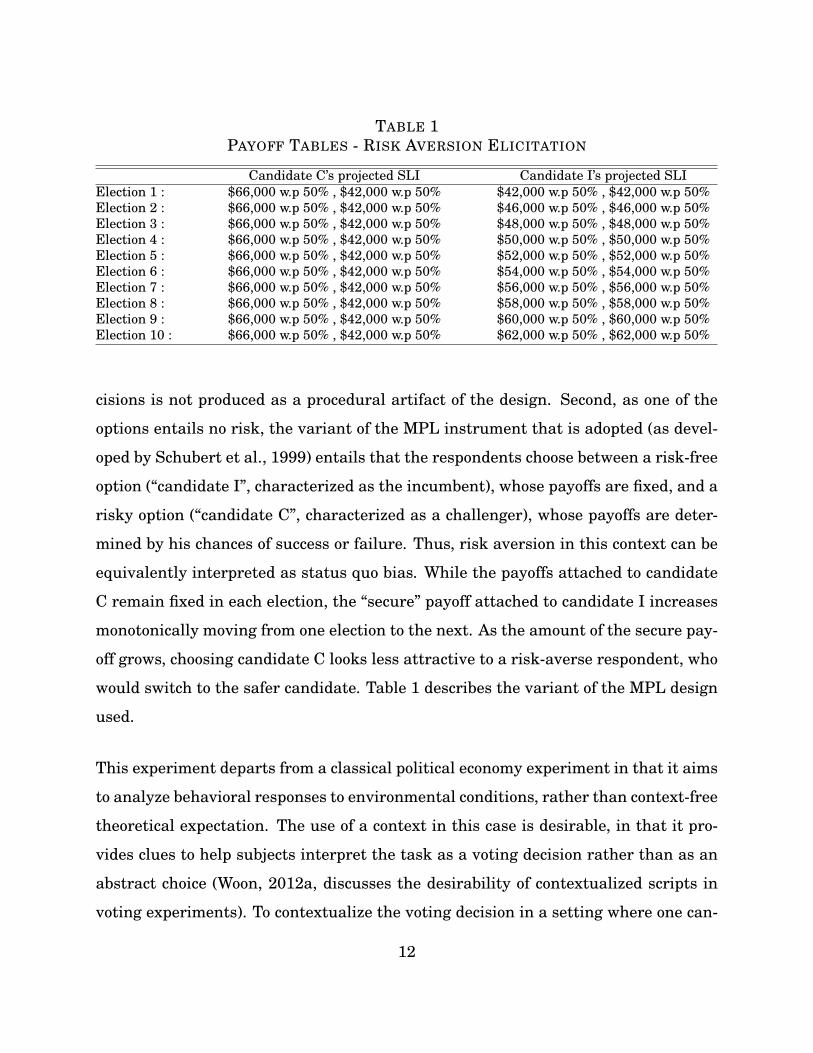
TABLE 1PAYOFF TABLES - RISK AVERSION ELICITATION

Candidate C’s projected SLI Candidate I’s projected SLIElection 1 : $66,000 w.p 50% , $42,000 w.p 50% $42,000 w.p 50% , $42,000 w.p 50%Election 2 : $66,000 w.p 50% , $42,000 w.p 50% $46,000 w.p 50% , $46,000 w.p 50%Election 3 : $66,000 w.p 50% , $42,000 w.p 50% $48,000 w.p 50% , $48,000 w.p 50%Election 4 : $66,000 w.p 50% , $42,000 w.p 50% $50,000 w.p 50% , $50,000 w.p 50%Election 5 : $66,000 w.p 50% , $42,000 w.p 50% $52,000 w.p 50% , $52,000 w.p 50%Election 6 : $66,000 w.p 50% , $42,000 w.p 50% $54,000 w.p 50% , $54,000 w.p 50%Election 7 : $66,000 w.p 50% , $42,000 w.p 50% $56,000 w.p 50% , $56,000 w.p 50%Election 8 : $66,000 w.p 50% , $42,000 w.p 50% $58,000 w.p 50% , $58,000 w.p 50%Election 9 : $66,000 w.p 50% , $42,000 w.p 50% $60,000 w.p 50% , $60,000 w.p 50%Election 10 : $66,000 w.p 50% , $42,000 w.p 50% $62,000 w.p 50% , $62,000 w.p 50%

cisions is not produced as a procedural artifact of the design. Second, as one of the

options entails no risk, the variant of the MPL instrument that is adopted (as devel-

oped by Schubert et al., 1999) entails that the respondents choose between a risk-free

option (“candidate I”, characterized as the incumbent), whose payoffs are fixed, and a

risky option (“candidate C”, characterized as a challenger), whose payoffs are deter-

mined by his chances of success or failure. Thus, risk aversion in this context can be

equivalently interpreted as status quo bias. While the payoffs attached to candidate

C remain fixed in each election, the “secure” payoff attached to candidate I increases

monotonically moving from one election to the next. As the amount of the secure pay-

off grows, choosing candidate C looks less attractive to a risk-averse respondent, who

would switch to the safer candidate. Table 1 describes the variant of the MPL design

used.

This experiment departs from a classical political economy experiment in that it aims

to analyze behavioral responses to environmental conditions, rather than context-free

theoretical expectation. The use of a context in this case is desirable, in that it pro-

vides clues to help subjects interpret the task as a voting decision rather than as an

abstract choice (Woon, 2012a, discusses the desirability of contextualized scripts in

voting experiments). To contextualize the voting decision in a setting where one can-

12

TABLE 2RISK AVERSION ELICITATION - PROSPECTS

Positive Prospect Negative ProspectOther 4 nations’ SLI Other 4 nations’ SLI

Election 1 : $42,000 $66,000Election 2 : $42,000 $66,000Election 3 : $42,000 $66,000Election 4 : $42,000 $66,000Election 5 : $42,000 $66,000Election 6 : $42,000 $66,000Election 7 : $42,000 $66,000Election 8 : $42,000 $66,000Election 9 : $42,000 $66,000Election 10 : $42,000 $66,000

didate is considered more risky than the other, the two candidates have been labeled

as “challenger” and “incumbent”, respectively.4

Payoffs were decided by a fair throw of a twenty-sided die and a coin. In Election 1,

the first (second) payoff is paid if the subjects has chosen candidate C and the coin

has landed heads up (down); the third (fourth) payoff is paid if the subject has chosen

candidate I and the coin has landed heads up (down).

As one proceeds down the matrix, the payoffs and attached probabilities of candidate

C remain the same, but the payoffs attached to candidate I change. The matrix of

ten election scenarios for each prospect is designed in such a way that only extremely

risk-seeking subjects choose candidate C in the last row, and only extremely risk-

averse subjects choose candidate I in the first few rows.5 A risk-neutral subject would

choose candidate C as long as the expected utility of candidate C is higher than the

expected utility of candidate I (in the first five elections), and candidate I otherwise

4A manipulation check treatment with abstract candidate labels has been run to test for possi-ble framing effects. The results show no significant difference between the framed and the abstracttreatment.

5Notice that rational players should always choose candidate C in the first election, because itweakly dominates the alternative option: it never yields a lower payoff and it yields a strictly largerpayoff with a positive probability. Thus the first election is considered as a control that the subject hasunderstood the instructions.

13

(last 4 elections).

Table 2 describes the design used for the prospect treatments. While payoffs remain

exactly identical to the ones described in Table 1, gain and loss domains are created

by contextualizing the voting decision internationally. The subjects are given infor-

mation about the relative wealthiness of other comparable countries by making the

other countries appear to be the reference point.

5 Prospect treatment results

I now investigate the effect of prospects on voting decisions (e.g., hypotheses 1, 2 and

3). Figure 1 reports the raw results of the prospect treatment. Consistent with the

extant literature, subjects display a considerable degree of risk aversion in the posi-

tive prospect, in that they switch from the risky to the safer candidate much earlier

than would a risk neutral agent. As shown by Figure 1, in election 6, around 75% of

the subjects vote for the safer candidate, as against 25% for the risky candidate, even

though the two candidates are identical in terms of expected utility (e.g., hypothesis

1). Even when the safer candidate yields a lower expected utility (election 5), subjects

still prefer to vote for him rather than for the risky candidate (around 65% of the

subjects vote for the safer candidate).Subjects seem, however, to also be risk-averse in the negative prospect. Figure 1

shows that in election 6, around 70% of the subjects vote for the safer candidate, con-

tradicting hypothesis 3. However, the likelihood of choosing the safer candidate seems

to be larger in the gain domain than in the loss domain in nearly every election (e.g.,

hypothesis 2), even though the domain’s effect seems to be more modest, as compared

to the previous studies of Quattrone and Tversky (1988). This variance is caused by

a difference of incentives that the subjects face between this experiment and those

in Quattrone and Tversky. As reported by Laury and Holt (2008)6, the use of real6Despite the widespread references to prospect theory in theoretical and experimental work, few

14

Probabilityof voting for the Incumben

t

0

0.1

0.2

0.3

0.4

0.5

0.6

0.7

0.8

0.9

1

1 2 3 4 5 6 7 8 9 10

Positive ProspectNegative Prospect

Elections

FIG. 1 - The effect of prospects: the vertical axis reports the percentage of votes for candidateI. The horizontal axis reports the election number. The blue line refers to observations in thedomain of positive prospects, while the red line refers to the domain of negative prospects.

incentives dramatically reduces the incidence of reflection behavior around the refer-

ence point. However, considering that the positive or negative domain does not affect

the subjects’ earnings, by inducing only a psychological framing, the results provide

support for the prospect theory: subjects are less risk-averse in the loss treatment

than in the gain treatment.

To test whether the effect of prospect (e.g., hypothesis 2) shown in Figure 1 is sta-

tistically significant, I calculated the average frequencies of votes for candidate I

(the safer choice) across all subjects for the two prospect treatments. Across all ten

elections, subjects vote for the safer candidate on average 5.96 times in the positive

prospect, and 5.55 times in the negative prospect. The difference is statistically sig-

studies have tested the theory with incentivized tasks (Kahneman and Tversky, 1979 and Tverskyand Kahneman, 1992 are based on hypothetical payoffs). Laury and Holt (2008) use a simple tool tomeasure risk preferences directly, based on a series of lottery choices with significant money payoffs inparallel gain and loss treatments.

15

nificant according to a Welch test, which tests the null hypothesis that the average

number of votes for the safer candidate in the negative prospect (µneg) exceeds the

average number of votes in the positive prospect (µpos). Denoting as σ2µneg

and σ2µpos

the

estimated variances of the average of the votes for candidate I in the negative and

positive prospect respectively, the test statistic has a t-distribution under the null

hypothesis.7

µneg − µpos√σ2µneg

+ σ2µpos

With a p-value=0.0179, the alternative hypothesis that the average of votes for the

incumbent in the positive prospect is larger than the average of votes in a negative

prospect cannot be rejected.

6 Weather treatment results

To investigate the effect of weather on voting (e.g., hypothesis 4), three definitions of

weather quality are used to characterize the actual weather on the day of the experi-

ment.

The amount of sunlight is the primary measure for the weather condition. Data

were collected on how many minutes the sky was clear, partly cloudy, and overcast

for the ZIP code of the city in which the experiment was conducted. The website

of Weather Underground (www.wunderground.com) offers detailed historical data on

intra-daily weather conditions for most ZIP codes in the United States. Accordingly,

a good weather day is defined as one in which the sky was clear for the majority of

the time, i.e. for more than 50% of the time between 7 a.m. and the time of the end of

the experiment. This measure will be referred to as the “clear/overcast” measure.

7The number of degrees of freedom of the t-distribution is(Nneg−1)(Npos−1)

(σ2µneg

−σ2µpos

)(Npos−1)σ4

µneg+(Nneg−1)σ4

µpos

, where Nneg

and Npos are the sample sizes of the two prospect treatments.

16

0

0.1

0.2

0.3

0.4

0.5

0.6

0.7

0.8

0.91

12

34

56

78

910

Goo

d weather

Bad weather

0.91

POSITIVE PROSPECTSubjectiv

e

Subjectiv

e

0

0.1

0.2

0.3

0.4

0.5

0.6

0.7

0.8

0.91

12

34

56

78

910

Overcast/Clear

0.91

Overcast/Clear

0

0.1

0.2

0.3

0.4

0.5

0.6

0.7

0.8

0.91

12

34

56

78

910

Precipita

tion

0.91

Precipita

tion

0

0.1

0.2

0.3

0.4

0.5

0.6

0.7

0.8

0.91

12

34

56

78

910

NEGATIVE PROSPECT

0

0.1

0.2

0.3

0.4

0.5

0.6

0.7

0.8

0.91

12

34

56

78

910

0

0.1

0.2

0.3

0.4

0.5

0.6

0.7

0.8

0.91

12

34

56

78

910

FIG

.2

-T

heef

fect

ofw

eath

er:

the

vert

ical

axis

repo

rts

the

perc

enta

geof

vote

sfo

rca

ndid

ate

I.T

heho

rizo

ntal

axis

repo

rts

the

elec

tion

num

ber.

Inea

chpa

nel,

the

blue

line

repr

esen

ts“g

ood

wea

ther

”da

ta,w

hile

the

red

line

refe

rsto

“bad

wea

ther

”da

ta.

The

top

pane

lref

ers

toob

serv

atio

nsin

the

posi

tive

pros

pect

trea

tmen

t,w

hile

the

bott

ompa

nelr

efer

sto

obse

rvat

ions

from

the

nega

tive

pros

pect

trea

tmen

t.O

bser

vati

ons

are

grou

ped

acco

rdin

gto

the

wea

ther

mea

sure

s.T

hepl

ots

onth

ele

ftre

fer

tosu

bjec

tive

wea

ther

asse

ssm

ent;

the

ones

inth

ece

nter

,to

clea

r/ov

erca

stm

easu

re;t

heon

eson

the

righ

t,to

the

prec

ipit

atio

nm

easu

re.

17

Because the subjective component plays a key role in assessing the perceived quality

of weather, the answers to the question “How do you feel about the weather today?”

provided in the questionnaire was used as a subjective measure of good/bad weather.

Specifically, subjects were asked to answer this question on a scale from 1 to 7, where

1 is “Terrible” and 7 is “Awesome.” Subjects were pooled into three groups: those who

provided an assessment of weather between 1 and 3; those who provided a neutral

assessment of 4; and those who provided a weather assessment between 5 and 7.

With this measure, I focus on the differences between the first group, who perceived

the weather as “good”, and the third group, who assesses the weather conditions as

being “bad”. This measure will be referred to as “subjective” measure.

Finally, precipitation provides another indicator of the quality of weather in any given

day. Accordingly, a rainy day is defined as one in which the amount of rainfall exceeds

the daily average amount in the area in which the experiment was conducted (which

is 0.12 inches per day). According to this measure, a rainy day is a bad weather

day. This assessment of the weather condition is referred to as the “precipitation”

measure.

Figure 2 reports the raw data of the effect of weather. This figure shows the exper-

imental distribution of the safer choice, i.e. candidate I, in each of the 10 elections.

Observations are pooled according to the three measures of weather assessment: the

subjective measure in the first column, the clear/overcast in the second column, and

the precipitation measure in the last column. Good weather is represented by a blue

line and bad weather by a red line. Note that in this figure greater risk aversion

implies a leftward shift of the frequency line.

The top panel refers to observations in a domain of “positive outcomes,” while the

bottom panel refers to observations in a domain of “negative outcomes.”

The plots of raw data suggest support for hypothesis 4: good weather increases the

likelihood of voting for the risky candidate, and this happens for all three measures

18

TABLE 3AVERAGE FREQUENCIES OF VOTES FOR CANDIDATE I

Subjective Clear/overcast PrecipitationPositive Prospect

Good Weather 5.66 5.48 5.82Bad Weather 6.45 6.25 6.55[p− values] [0.0054] [0.0034] [0.0177]

Negative ProspectGood Weather 5.19 5.06 5.40Bad Weather 6.11 5.85 6.18[p− values] [0.0015] [0.0027] [0.0109]

Notes - The table reports the mean across all subjects of the average number of votes forcandidate I (the safer candidate) across the ten elections conditional on good and bad weatherconditions. The definitions of weather conditions are reported in the first row of the table.The numbers in the squared brackets represent the p-values of the Welch test for the nullhypothesis that the mean in good weather conditions is larger than the mean in bad weatherconditions.

of weather conditions adopted. The impact of weather is particularly pronounced for

decisions 3 to 7, the marginal decisions, where the majority of subjects start switching

from the riskier to the safer lottery.

Are the differences in voting choice documented in Figure 2 statistically significant?

To assess the validity of my hypothesis, I calculated the average frequencies of votes

for candidate I (the safer choice) across all subjects and for the three definitions of

weather that I adopted. The results of the experiment are strikingly clear: good

weather promotes greater propensity to vote for the risky candidate. These differ-

ences are shown to be statistically significant. The null hypothesis that the average

number of safe choices in good weather (µgood) exceeds the average number of safe

choices in bad weather (µbad) can be tested using the Welch test, as is done in the

previous section. Based on the low p-values reported in Table 3, the alternative hy-

pothesis that the average of votes for the safer candidate with bad weather is larger

than the average of votes with good weather cannot be rejected. Similar results are

shown for the negative prospect.

19

TABLE 4VOTES FOR CANDIDATE I – POSITIVE PROSPECT

Precipitation Overcast-Clear Subjective WeatherIntercept 6.149 5.848 5.916

[0.204] [0.200] [0.207]

Bad-Good Weather 0.355∗∗ 0.392∗∗∗ 0.434∗∗∗

[0.161] [0.082] [0.138]

Gender −0.821∗∗∗ −0.857∗∗∗ −0.849∗∗∗(Male-Female) [0.243] [0.205] [0.241]

Race 0.004 0.061 0.128(White-Black) [0.100] [0.079] [0.092]

Income 0.340∗ 0.320∗∗ 0.379∗∗∗

[0.181] [0.142] [0.119]

Religious −0.038 0.002 0.004(Yes-No) [0.108] [0.111] [0.111]

Political Leaning 0.051 −0.022 0.067(Liberal-Conservative) [0.171] [0.153] [0.177]

Notes - The table reports the estimated coefficients of the regressions of the number of votesfor candidate I (the safer candidate) on a dummy variable which is equal to 1 when theweather is bad and -1 when the weather is good. The numbers in square brackets are thestandard errors of the estimated coefficients. One star, two stars, and three stars refer tostatistical significance at the 1, 5 and 10 percent levels, respectively.

7 Further Controls

To investigate whether the results are led by confounding variables, such as personal

characteristics and socio-economic attitudes, the total number of votes for candidate I

is regressed on dummy variables representing each of the weather-related variables,

plus additional controls.

The explanatory variables used as control are reported in the first column of Tables 4

and 5.8 All the weather-related variables appear to be strongly statistically signif-

icant at conventional confidence levels. The only socio-economic controls that are

significant in the positive prospect are gender (women display less tolerance to risk

8A gender dummy equals 1 if male, and -1 if female; a race dummy equals 1 if white, and -1 if black,an income variable is expressed in U.S. dollars; a religiousness dummy equals 1 if the subject self-declared as religious person, and -1 otherwise; and a political leaning dummy equals 1 if the subjectself-declared as liberal or most liberal, and -1 if conservative or most conservative).

20

TABLE 5VOTES FOR CANDIDATE I – NEGATIVE PROSPECT

Precipitation Overcast-Clear Subjective WeatherIntercept 5.935 5.599 5.667

[0.258] [0.223] [0.209]

Bad-Good Weather 0.421∗∗∗ 0.398∗∗∗ 0.451∗∗

[0.117] [0.116] [0.176]

Gender −0.341 −0.385∗ −0.376(Male-Female) [0.256] [0.222] [0.247]

Race −0.240∗∗ −0.173 −0.103(White-Black) [0.098] [0.118] [0.141]

Income 0.152 0.125 0.186[0.164] [0.176] [0.156]

Religious −0.146 −0.104 −0.127(Yes-No) [0.112] [0.117] [0.153]

Political Leaning −0.057 −0.133 −0.042(Liberal-Conservative) [0.201] [0.188] [0.210]

Notes - The table reports the estimated coefficients of the regressions of the number of votesfor candidate I (the safer candidate) on a dummy variable which is equal to 1 when theweather is bad and -1 when the weather is good. The numbers in square brackets are thestandard errors of the estimated coefficients. One star, two stars, and three stars refer tostatistical significance at the 1, 5 and 10 percent levels, respectively.

as also found by Eckel and Grossman, 2007) and income (risk aversion– or status quo

bias –seems to increase with the level of wealth). No control is significant across all

the weather measures in the negative prospect treatment.

7.1 Causal pathway

The underlining hypothesis of this experiment is that mood is the intermediate vari-

able that determines the shift in risk tolerance that we detect in this analysis. Here,

I investigate the effect of weather on mood (e.g., hypothesis 5) by using the responses

that the subjects provided to a psychological questionnaire called PANAS-X (Watson

and Clark 1994).

The PANAS-X methodology, which is widely used in psychology literature, uses two

main scales to measure positive and negative affects, the dominant dimensions of

21

emotional experience. Positive affect is defined as feelings that reflect a level of plea-

surable engagement with the environment, such as happiness, joy, excitement, enthu-

siasm, and contentment (Clark, Watson, and Leeka, 1989). Negative affect measures

feelings such as fear, anger, anxiety, and depression. In addition to the two higher-

order scales, the PANAS-X measures eleven specific affects: fear, sadness, guilt, hos-

tility, shyness, fatigue, surprise, joviality, self-assurance, attentiveness, and serenity.

The Appendix reports the questionnaire as it was presented to the subjects.

The scale consists of a number of words and phrases that describe different feelings

and emotions, such as cheerful, sad, and active. Subjects were required to assess on

a scale from 1 to 5 the extent to which they had felt each feeling and emotion during

the day of the experiment. The individual scores for each feeling were added within

each mood category and re-scaled on a 0-1 scale.

Table 6 reports the differences of the scores between bad and good weather for all the

PANAS-X mood characteristics. A positive number in this table means that the score

is larger with bad weather, whereas a negative number means that the score is larger

with good weather. The results suggest that amount of sunlight, my primary mea-

sure for the weather condition, has an effect on the extent of overall positive feelings

(displayed by the higher-order scale), and less of an effect on the extent of negative

feelings. As regards as specific affect states, feelings of self-assurance and attentive-

ness demonstrate a statistically significant increase in good weather conditions. The

only negative affect feeling that displays a significant difference in the two weather

treatment is sadness, which appears to be larger in bad weather conditions. Fatigue

and serenity, also display significant differences in the weather treatments, with the

former being significantly more pronounced in bad weather conditions, and the latter

being higher in good weather days.

I investigate the importance of mood as an explanation of the results (e.g., hypothesis

6), by regressing the total number of votes for the risk-free candidate, across the

22

TABLE 6PANAS TEST

Panel A: General Dimensions ScalesClear/Overcast Precipitation Subjective Weather

Negative Affect 0.010 0.003 0.036[0.301] [0.436] [0.034]

Positive Affect −0.129 −0.032 −0.063[0.000] [0.218] [0.077]

Panel B: Basic Negative Emotion ScalesClear/Overcast Precipitation Subjective Weather

Fear 0.024 0.036 0.048[0.139] [0.079] [0.041]

Hostility −0.011 0.020 −0.014[0.344] [0.184] [0.171]

Guilt −0.018 −0.013 −0.012[0.294] [0.222] [0.234]

Sadness 0.045 −0.013 0.063[0.011] [0.284] [0.019]

Panel C: Basic Positive Emotion ScalesClear/Overcast Precipitation Subjective Weather

Joviality −0.037 0.004 −0.040[0.181] [0.464] [0.196]

Self-Assurance −0.127 −0.004 −0.072[0.001] [0.469] [0.056]

Attentiveness −0.126 −0.033 −0.097[0.000] [0.201] [0.014]

Panel D: Other Affective StatesClear/Overcast Precipitation Subjective Weather

Shyness −0.050 −0.031 0.020[0.091] [0.061] [0.241]

Fatigue 0.135 0.000 0.135[0.007] [0.498] [0.008]

Serenity −0.132 −0.049 −0.059[0.003] [0.135] [0.114]

Surprise 0.013 0.025 −0.017[0.373] [0.279] [0.345]

Notes - Each entry reports the spread of the scores between the bad and the good weathercondition in the corresponding column. The numbers in squared brackets represent the p-values for the null hypothesis that the average score in bad weather conditions is smallerthan the average score in good weather conditions (when the spread is positive) or that theaverage score in bad weather conditions is larger than the average score in good weatherconditions (when the spread is negative).

23

prospect treatments discussed above, on the PANAS-X scores in the feelings that

are displayed to be significantly affected by weather as shown in Table 6. Table 7

reports the findings. The results are clear: Positive feelings decrease the likelihood of

choosing the safer choice; or, equivalently, better mood promotes risk-taking behavior.

This effect appears to be statistically significant at the conventional levels.

The middle panel of Table 7 sheds additional light on the plausibility of mood changes

as a pathway for the described effect of weather on human behavior.9 Mood is decom-

posed into a weather-related component, namely, the projection of the six PANAS-X

mood categories reported in the table on the three weather variables defined in Sec-

tion 3, and a non-weather related component, that is, the residual of the regression.

Overall, mood accounts for around 10% of the observed decision-making behavior (see

“Total R2”), and weather accounts for a large fraction of it (see “Weather Mood R2”).

This evidence suggests an explanation of the experimental results in terms of the sub-

jects being more or less in a good mood and therefore more or less willing to accept

the risks at stake in the experimental treatment.

The mood-risk channel that is established in this paper is not mutually exclusive with

other cognitive biases or with other channels through which mood affects individuals’

behavior. The PANAS-X questionnaire shows that not all mood states are affected by

weather. Mood states such as “joviality” (including happiness, joyfulness, delightful-

ness, cheerfulness, excitedness, enthusiasm, and liveliness) or “hostility” (including

anger, hostility, irritability, scornfulness, and loath) are not found to be affected by

weather conditions, but might strongly affect voters’ behavior. A growing literature

analyzes the effect of these mood states on individual political actions and attitudes.

For instance, Healy et al (2010) analyze the effect of happiness generated by the per-

formance of local sport franchises on the likelihood of re-electing the incumbent and

on the presidential approval rating, finding that higher performances affect positively

9Table A.3 shows the effect of other mood affect states on the participants’ voting decisions.

24

TABLE 7MOOD, WEATHER, AND VOTING

Positive Self- Attentiveness Sadness Fatigue SerenityAffect Assurance

Intercept 11.371 11.371 11.371 11.371 11.371 11.371[0.476] [0.487] [0.483] [0.505] [0.505] [0.485]

Mood −0.519∗∗ −0.412 −0.367∗∗ −0.145 −0.156 −0.510∗∗∗[0.240] [0.294] [0.185] [0.438] [0.167] [0.194]

Total R2 0.105 0.077 0.103 0.026 0.116 0.097

Weather Mood R2 0.101 0.075 0.102 0.021 0.098 0.092

Non-Weather Mood R2 0.003 0.002 0.000 0.005 0.018 0.005

Notes - The top panel reports the estimated coefficients of the regressions of the combinednumber of votes for the safer candidate in the two prospect treatments on an intercept andon the standardized scores of the PANAS-X categories reported on the first row. The numbersin square brackets are the standard errors of the estimated coefficients. One star, two stars,and three stars refer to statistical significance at the 1, 5 and 10 percent levels, respectively.In the bottom panel, mood is divided into a weather-related component, the projection of thestandardized scores of the PANAS-X categories reported on the first row on the three weatherdummies defined in Section 3, and a non-weather related component, the residual. Total R2

refers to the R2 of the regressions of votes for the safe candidate on both weather and nonweather related components, while Weather Mood R2 and Non-Weather Mood R2 refer to thevariance explained by the two subcomponents.

the likelihood of re-electing the incumbent or ratings of the president’s performance;

Miller (2013) analyzes the effect of professional sports records on incumbent mayoral

elections, finding that winning sports records boost incumbents’ vote totals.

8 Conclusions

An increasing number of media outlets have recently focused on the effect of weather

on U.S. elections, claiming that inclement weather favors the Republican candidates.

No consensus exists, however, in either the theoretical or the empirical literature

about the net effect of inclement weather on an election day. It is not clear who the

marginal voter is that the weather deters from turning out, or what the final effect of

weather is on elections’ outcomes.

25

This paper provides an alternative analysis of the effect of weather on voters’ de-

cisions, not by examining the decision to turnout, but rather by investigating the

decision-making activity of the voters who do turn out. The impact of weather on

human mood and hence on decision-making activity has been widely examined in the

psychology literature. Bassi et al (2013) show that weather (through the intermediate

variable of mood) affects risk preferences and, thus, the degree with which individ-

uals are tolerant to risk. A growing stream of literature has begun to analyze how

risk and uncertainty affects voters’ actions and preferences. This paper tackles this

question by analyzing a specific aspect of uncertainty, the risk attached to the future

performance of the candidates running in the election. Quattrone and Tversky (1988)

test a similar scenario, confirming that, with all else being equal, voters display a

significant degree of risk aversion in choosing less risky candidates.

The paper provides experimental evidence of the effect of weather– measured in terms

of precipitation, sunlight exposure, and subjective assessment –on the likelihood that

individuals will vote for the candidate who is perceived to be less risky. After measur-

ing bad and good weather conditions with a large set of variables, findings show that

bad weather decreases risk tolerance, thus increasing the likelihood of voting in favor

of the risk-free candidate, while good weather conditions promote risk-taking behav-

ior. In “marginal elections,” in which a voter is likely to consider whether to switch

from a riskier to the safer candidate, bad weather may result in up to a twice-as-large

probability of choosing the safer candidate over the risky one.

Although the abstract setting of this experiment can hardly explain voting behavior

in all kinds of political elections (where partisanship, political attitudes, and informa-

tion about candidates vary), these findings provide an initial step to understanding

the effect of weather and mood on voting choice.

The results of this analysis suggest that not only policy ambiguity (as most commonly

explored in the literature) but also performance uncertainty might be an important

26

factor in determining voters’ choices, especially when candidates’ policy preferences

are perceived to be close enough. This opens up new questions to pursue to advance

our collective understanding of risks and their effect on individual decision-making

activity and voting: what kind of individual characteristics or personal and profes-

sional experiences make a candidate perceived to be more or less risky by the voters?

What kind of risks are voters more sensible to, and what risks they are more willing

to tolerate?

Moreover, the paper sheds light on the effect of mood on voting choice, by distinguish-

ing between affect states and by differentiating feeling states. Employing a design

that measures participants’ mood states, this study is not only able to indicate pre-

cisely the mood states that are sensible to weather conditions, but also the direct

effect of these mood states on voting behavior. Further analysis of the effect of mood

states on risk tolerance would advance the understanding of variation in human be-

havior not only in political settings, but also in economics, sociology, and finance.

27

ReferencesAlvarez, Michael R. and Charles H. Franklin. (1994). “Uncertainty and Political Percep-tions,” Journal of Politics, 56(3), 671—688.

Bartels, Larry M. (1998). “Issue Voting under Uncertainity: An Empirical Test,” AmericanJournal of Political Science, 30, 709—728.

Bassi, Anna, Riccardo Colacito and Paolo Fulghieri. (2013). “’O Sole Mio: An Experi-mental Analysis of Weather and Risk Attitudes in Financial Decisions,” Review of FinancialStudies, forthcoming.

Berinsky, Adam J. and Jeffrey B. Lewis. (2007). “An Estimate of Risk Aversion in theU.S. Electorate,” Quarterly Journal of Political Science, 2, 139—154.

Bernulli, Daniel. (1954). “Exposition of a New Theory on the Measurement of Risk.” Econo-metrica, 22(1), 23—36.

Clark, Lee Anna, David Watson, and Jay Leeka. (1989). “Diurnal Variation in the Posi-tive Affects,” Motivation and Emotion, 13, 205—34.

Cohen, Alexander. (2011). “The Photosynthetic President: Converting Sunshine into Popu-larity,” The Social Science Journal, 48, 295—304.

Cunnigham, Michael R. (1979). “Weather, Mood, and Helping Behavior: Quasi-experimentswith Sunshine Samaritan,” Journal of Personality and Social Psychology, 37, 1947—1956.

DeNardo, James. (1980). “Turnout and the Vote: The Joke’s on the Democrats.” The Ameri-can Political Science Review, 74(2), 406—420.

DeSteno, David, Richard Petty, Derek D. Rucker, and Duane T. Wegener. (2000).“Beyond Valence in the Perception of Likelihood: The Role of Emotion Specificity,” Journal ofPersonality and Social Psychology, 78, 397—416.

Denissen, Jaap J.A., Ligaya Butalid, Lars Penke, and Marcel A. G. van Aken. (2008).“The Effects of Weather on Daily Mood: A Multilevel Approach,” Emotion, 8(5) 662—67.

Druckman, James N. (2001a). “Evaluating Framing Effects,” Journal of Economic Psychol-ogy, 22, 91—101.

Druckman, James N. (2001b). “On the Limits of Framing Effects: Who Can Frame?,” Jour-nal of Politics, 63(4), 1041—66.

Druckman, James N. (2001c). “The Implications of Framing Effects for Citizen Compe-tence,” Political Behavior, 23(3), 225—256.

Druckman, James N. and Rose McDermott. (2008). “Emotion and the Framing of RiskyChoice,” Political Behavior, 30, 297—321.

28

Eckel, Catherine C. and Philip J. Grossman. (2007). “Men, Women and Risk Aversion:Experimental Evidence,” in Handbook of Experimental Results, ed. by C. Plott, and V. Smith,North Holland. Elsevier Science.

Eckel, Catherine C, Mahmoud A. El-Gamalb, and Rick K. Wilson. (2009). “Risk Lov-ing after the Storm: A Bayesian-Network Study of Hurricane Katrina Evacuees” Journal ofEconomic Behavior and Organization, 69, 110—124.

Eisenberg, Amy, Jonathan Baron, and Martin E.P. Seligman. (1998). “Individual Dif-ferences in Risk Aversion and Anxiety,” Psychological Bulletin, 87, 245—51.

Enelow, James, and Melvin J. Hinich. (1981). “A new approach to voter uncertainty inthe Downsian spatial model,” American Journal of Political Science, 25, 483—93.

Feldman, Stanley, Leonie Huddie, and Erin Cassese. (2013). “The Role of Emotion inPolitical Cognition,” in Grounding Social Sciences in Cognitive Sciences, ed. by Ron Sun,North Holland. MIT Press, forthcoming.

Gatrell, Jay D., and Gregory D. Bierly. (2002). “Weather and Voter Turnout: KentuckyPrimary and General Elections 1990-2000,” Southeastern Geographer, 42, 114—134.

Gerber Elisabeth. (2013). “Partisanship and Local Climate Policy,” Cityscape, Spring 2013,forthcoming.

Goldstein, Kenneth M. (1972). “Weather, Mood, and Internal-External Control,” PerceptualMotor Skills, 35, 786.

Gomez, Brad T., Thomas G. Hansford, and George A. Krause. (2007). “The RepublicansShould Pray for Rain: Weather, Turnout, and Voting in U.S. Presidential Elections.” TheJournal of Politics, 69(3), 647—661.

Healy, Andrew and Neil Malhotra. (2010). “Random Events, Economic Losses, and Ret-rospective Voting: Implications for Democratic Competence,” Quarterly Journal of PoliticalScience, 5, 193—208.

Heath, Chip, Richard P. Larrick, and George Wu. (1999). “Goals as Reference Points,”Cognitive Psychology, 38, 79—109.

Holt, Charles A., and Susan K. Laury. (2002). “Risk Aversion and Incentive Effects,” TheAmerican Economic Review, 92(5), 1644—1655.

Howarth, E., and M.S. Hoffman. (1984). “A Multidimensional Approach to the Relationshipbetween Mood and Weather,” British Journal of Psychology, 75, 15—23.

Hsee, Christopher K., and Elke U. Weber. (1997). “A Fundamental Prediction Error: Self-other Discrepancies in Risk Reference,” Journal of Experimental Psychology, 126, 45—53.

Huddy, Leonie, Stanley Feldman, and Erin Cassese. (2007). “On the Distinct Political

29

Effects of Anxiety and Anger,” in The Affect Effect, ed. by Ann Crigler, Michael MacKuen,George E. Marcus, and W. Russell Neuman, University of Chicago Press.

Johnson, Eric and Amos Tversky. (1983). “Affect, Generalization, and the Perception ofRisk,” Journal of Personality and Social Psychology, 45, 20—31.

Kahneman, Daniel and Amos Tversky. (1979). “Prospect Theory: An Analysis of ChoiceUnder Risk, Econometrica, 47(2), 263—291.

Keele, Luke, and Jason Morgan. (2013). “Stronger Instruments By Design,” mimeo.

Keller, Matthew C., Barbara L. Fredrickson, Oscar Ybarra, Stephane Cote, KareemJohnson, Joe Mikels, Anne Conway, and Tor Wager. (2005). “A Warm Heart and a ClearHead. The Contingent Effects of Weather on Mood and Cognition,” Psychological Science,16(9), 724—731.

Knack, Steve. (1994). “Does Rain Help the Republicans? Theory and Evidence on Turnoutand the Vote,” Public Choice, 79, 187—209.

Laury, Susan K., and Charles A. Holt. (2008). “Further Reflections on Prospect Theory,”in J.C. Cox and G. W. Harrison, eds.: Risk Aversion in Experiments. Research in ExperimentalEconomics, volume 12 (Bingley, U: Emerald).

Ludlum, David M. (1984). “The Weather Factor”. Boston: American Meteorological Society.

McDermott, Rose. (2001). “The Psychological Ideas of Amos Tversky and their Relevancefor Political Science.” Journal of Theoretical Politics, 13(1), 5—33.

MacKuen, Michael, Jennifer Wolak, Luke Keele and George E. Marcus. (2010). “CivicEngagements: Resolute Partisanship or Reflective Deliberation,” American Journal of Politi-cal Science, 54(2), 440—458.

Miller, Louis, Meyer, David E., and John T. Lanzetta. (1969). “Choice Among EqualExpected Value Alternatives: Sequential Effects of Winning Probability Level on Risk Prefer-ence.” Journal of Experimental Psychology, 79(3), 419—423.

Miller, Michael. (2013). “For the Win! The Effect of Professional Sports Records on MayoralElections.” Social Science Quarterly, 94(1), 59—78.

Morgenstern, Scott, and Elizabeth Zechmeister. (2001). “Better the Devil You Knowthan the Saint You Don’t: Risk Propensity and Vote Choice in Mexico,” The Journal of Politics,63(1), 93-119.

Palfrey, Thomas R., and Keith T. Poole. (1987). “The Relationship Between Information,Ideology, and Voting Behavior,” American Journal of Political Science, 31(3), 511-30.

Parrot, Gerrod W., and John Sabini. (1990). “Mood and Memory under Natural Condi-tions: Evidence for Mood Incongruent Recall,” Journal of Personality and Social Psychology,

30

59, 321—336.

Quattrone, George A., and Amos Tversky. (1988). “Contrasting Rational and Psychologi-cal Analyses of Political Choice,” American Political Science Review, 82(3), 719—36.

Sanders, Jeffrey L., and Mary S. Brizzolara. (1982). “Relationships between Weatherand Mood,” Journal of General Psychology, 107, 155—156.

Schubert, Renate, Martin Brown, Matthias Gysler, and Hans Wolfgang Brachinger.(1999). “Financial Decision-making: Are Women Really more Risk-averse? ” American Eco-nomic Review, 89(2), 381—385.

Shepsle, Kenneth A. (1972). “The Strategy of Ambiguity: Uncertainty and Electoral Com-petition,” The American Political Science Review, 66, 555—68.

Tversky, Amos, and Daniel Kahneman. (1992). “Advances in Prospect Theory: Cumula-tive Representation of Uncertainty,” Journal of Risk and Uncertainty, 5, 297—323.

Watson, D., and L. A. Clark. (1994). “The PANAS-X: Manual for the Positive and NegativeAffect Schedule - Expanded Form,” The University of Iowa. Available at: http://ir.uiowa.edu/psychology pubs/11..

Woon, Jonathan. (2012a). “Democratic Accountability and Retrospective Voting: A Labora-tory Experiment.” American Journal of Political Science, 56(4), 913-930

Woon, Jonathan. (2012b). “Laboratory Tests of Formal Theory and Behavioral Inference,”in B. Kittel, W. Luhan, and R.B. Morton (eds): Experimental Political Science: Principles andPractices (Palgrave Macmillan).

Wright, William F. and Gordon H Bower. (1992). “Mood Effects on Subjective ProbabilityAssessment,” Organizational Behavior and Human Decision Processes, 52, 276—291.

31

On-line Appendix: Experimental procedures and Instructions

Subjects were recruited from the UNC e-recruit subject pool. Subjects had joined the sub-

ject pool voluntarily by completing a form on line indicating their interest in participating

in experiments. When a student enrolled for participation in the experiment, she was told

only that she would participate in an experiment about decision making under uncertainty.

When a subject entered the laboratory, she was given a card with a unique subject number,

which identified the subject during the experiment, she was given a consent form and she was

assigned to separate workplace, each far enough to others’ subjects workplace such that the

subjects could not see what the other subjects were doing, nor could they be seen by other

subjects.

After signing the consent form, subjects were given 20 sets of political scenarios, each rep-

resenting 20 different elections among two candidates the subjects needed to vote for with

monetary payoffs attached to every candidate. Instructions were given to the subjects along

with the 20 scenarios and they were read aloud. There was no time limit for the instructions

and subjects had the opportunity to ask questions in private. A monitor was present to answer

questions and to ensure that subjects did not communicate with each other. After the subjects

made their decisions, they were given the PANAS-X affect scale form to complete. When all

subjects had completed the PANAS-X form, experimental personnel went to each subject to

randomly determine their payoffs.10 Subjects were payed in private after completing their

own questionnaire and they could leave the room.

10Experimental personnel rolled 1 die first and then tossed a coin. First, a twenty-sided die deter-mined which of the twenty scenario was payoff-relevant. Second, the coin was used to determinedwhether which amount was payed out to them in the following way. If the coin landed heads up, sub-jects were paid a payoff equal to the forecast of expert 1 (for either candidate, depending who theychose), elsewhere they were paid the forecast of expert 2.

32

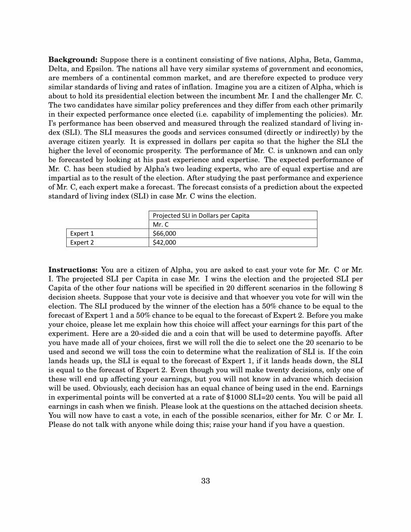
Background: Suppose there is a continent consisting of five nations, Alpha, Beta, Gamma,Delta, and Epsilon. The nations all have very similar systems of government and economics,are members of a continental common market, and are therefore expected to produce verysimilar standards of living and rates of inflation. Imagine you are a citizen of Alpha, which isabout to hold its presidential election between the incumbent Mr. I and the challenger Mr. C.The two candidates have similar policy preferences and they differ from each other primarilyin their expected performance once elected (i.e. capability of implementing the policies). Mr.I’s performance has been observed and measured through the realized standard of living in-dex (SLI). The SLI measures the goods and services consumed (directly or indirectly) by theaverage citizen yearly. It is expressed in dollars per capita so that the higher the SLI thehigher the level of economic prosperity. The performance of Mr. C. is unknown and can onlybe forecasted by looking at his past experience and expertise. The expected performance ofMr. C. has been studied by Alpha’s two leading experts, who are of equal expertise and areimpartial as to the result of the election. After studying the past performance and experienceof Mr. C, each expert make a forecast. The forecast consists of a prediction about the expectedstandard of living index (SLI) in case Mr. C wins the election.

Page | 1  

Background: 

Suppose  there  is a continent consisting of  five nations, Alpha, Beta, Gamma, Delta, and Epsilon. The nations all have very similar systems of government and economics, are members of a continental common market, and are therefore expected to produce very similar standards of  living and rates of  inflation. Imagine you are a citizen of Alpha, which is about to hold its presidential election between the incumbent Mr. I and the challenger Mr. C. The two  candidates  have  similar  policy  preferences  and  they  differ  from  each  other  primarily  in  their  expected performance once elected (i.e. capability of implementing the policies).  

Mr. I’s performance has been observed and measured through the realized standard of  living  index (SLI). The SLI measures the goods and services consumed (directly or indirectly) by the average citizen yearly. It is expressed in dollars per capita so that the higher the SLI the higher the level of economic prosperity.  

The performance of Mr. C. is unknown and can only be forecasted by looking at his past experience and expertise. The expected performance of Mr. C. has been studied by Alpha's two leading experts, who are of equal expertise and are  impartial as to the result of the election. After studying the past performance and experience of Mr. C, each expert make a forecast. The forecast consists of a prediction about the expected standard of living index (SLI) in case Mr. C wins the election. 

 

  Projected SLI in Dollars per Capita

  Mr. C 

Expert 1  $66,000 

Expert 2  $42,000 

 

Instructions: 

You are a citizen of Alpha, you are asked to cast your vote for Mr. C or Mr. I. The projected SLI per Capita in case Mr. I wins the election and the projected SLI per Capita of the other four nations will be specified in 20 different scenarios in the following 8 decision sheets. 

Suppose that your vote  is decisive and that whoever you vote for will win the election. The SLI produced by the winner of the election has a 50% chance to be equal to the forecast of Expert 1 and a 50% chance to be equal to the forecast of Expert 2. 

Before you make your choice, please let me explain how this choice will affect your earnings for this part of the experiment. Here are a 20‐sided die and a coin that will be used to determine payoffs. After you have made all of your choices, first we will roll the die to select one the 20 scenario to be used and second we will toss the coin to determine what the realization of SLI is. If the coin lands heads up, the SLI is equal to the forecast of Expert 1, if it lands heads down, the SLI is equal to the forecast of Expert 2. Even though you will make twenty decisions, only one of these will end up affecting your earnings, but you will not know in advance which decision will be used. Obviously, each decision has an equal chance of being used in the end. Earnings in experimental points will be converted at a rate of $1000 SLI=20 cents. You will be paid all earnings in cash when we finish.  Please  look at the questions on the 8 attached decision sheets. You will now have to cast a vote,  in each of the possible scenarios, either for Mr. C or Mr. I. Please do not talk with anyone while doing this; raise your hand if you have a question. 

 

  

Instructions: You are a citizen of Alpha, you are asked to cast your vote for Mr. C or Mr.I. The projected SLI per Capita in case Mr. I wins the election and the projected SLI perCapita of the other four nations will be specified in 20 different scenarios in the following 8decision sheets. Suppose that your vote is decisive and that whoever you vote for will win theelection. The SLI produced by the winner of the election has a 50% chance to be equal to theforecast of Expert 1 and a 50% chance to be equal to the forecast of Expert 2. Before you makeyour choice, please let me explain how this choice will affect your earnings for this part of theexperiment. Here are a 20-sided die and a coin that will be used to determine payoffs. Afteryou have made all of your choices, first we will roll the die to select one the 20 scenario to beused and second we will toss the coin to determine what the realization of SLI is. If the coinlands heads up, the SLI is equal to the forecast of Expert 1, if it lands heads down, the SLIis equal to the forecast of Expert 2. Even though you will make twenty decisions, only one ofthese will end up affecting your earnings, but you will not know in advance which decisionwill be used. Obviously, each decision has an equal chance of being used in the end. Earningsin experimental points will be converted at a rate of $1000 SLI=20 cents. You will be paid allearnings in cash when we finish. Please look at the questions on the attached decision sheets.You will now have to cast a vote, in each of the possible scenarios, either for Mr. C or Mr. I.Please do not talk with anyone while doing this; raise your hand if you have a question.

33

PANAS-X Test:

cheerful sad active angry at self

disgusted calm guilty enthusiastic

attentive afraid joyful downhearted

bashful tired nervous sheepish

sluggish amazed lonely distressed

daring shaky sleepy blameworthy

surprised happy excited determined

strong timid hostile frightened

scornful alone proud astonished

relaxed alert jittery interested

irritable upset lively loathing

delighted angry ashamed confident

inspired bold at ease energetic

fearless blue scared concentrating

disgusted

with self shy drowsy

dissatisfied

with self

This scale consists of a number of words and phrases that describe different

feelings and emotions. Read each item and then mark the appropriate

answer in the space next to that word. Indicate to what extent you have felt

this way today. Use the following scale to record your answers:

1 very slightly or not at all

2 a little

3 moderately

4 quite a bit

5 extremely

34

Classification of PANAS-X Categories:

General Dimension ScalesNegative Affect: afraid, scared, nervous, jittery, irritable, hostile, guilty, ashamed, upset, dis-tressedPositive Affect: active, alert, attentive, determined, enthusiastic, excited, inspired, interested,proud, strong

Basic Negative Emotion ScaleFear: afraid, scared, frightened, nervous, jittery, shakyHostility: angry, hostile, irritable, scornful , disgusted, loathingGuilt: guilty, ashamed, blameworthy, angry at self, disgusted with self, dissatisfied at selfSadness: sad, blue, downhearted, alone, lonely

Basic Positive Emotion ScaleJoviality: happy, joyful, delighted, cheerful, excited, enthusiastic, lively, energeticSelf-Assurance: proud, strong, confident, bold, daring, fearlessAttentiveness: alert, attentive, concentrating, determined

Other Affective StatesShyness: shy, bashful, sheepish, timidFatigue: sleepy, tired, sluggish, drowsySerenity: calm, relaxed, at easeSurprise: amazed, surprised, astonished

35

TABLE A.1DEMOGRAPHIC STATISTICS

1 2 3 4 5 6 7In what year were you born? 16.38 0.86 3.45 6.03 9.48 18.10 45.69(1=(-,80], 2=(80, 85], 3=(85,87], 4=(87,89],5=(89,90], 6=(90,91], 7=(91,+) )

Gender? 33.62 66.38(1=Male, 2=Female)

Racial or ethnic group 52.59 19.83 6.03 0.00 17.24 0.86 2.59(1=White, 2=Black, 3=Hispanic, 4=Am Indian,5=Asian, 6=Pacifi, 7=Multi )

Marital status 7.76 87.93 1.72 0.86 0.86(1=Married, 2=Single, 3=Divorced, 4=Widowed, 5=Other)

Current employment 11.21 23.28 49.14 6.03 9.48(1=Full-time outside, 2=Part-time outside, 3=Student,4=Research Assistant, 5=Other part time at school)

Major 22.41 6.03 56.03 15.52(1=Natural Sc, 2=Humanities, 3=Social Sc, 4=NA)

Current school year 9.48 20.69 24.14 18.97 11.21 0.86 13.79(1=Fr, 2=So, 3=Jr, 4=Sr, 5=Graduate, 6=Law, 7=NA)

Personal income 53.45 20.69 12.07 6.03 1.72 5.17(1=[0,5], 2=[6-15], 3=[16-30], 4=[31-45], 5=[46-60], 6=60+)

Family income 25.86 24.14 25.86 8.62 7.76 5.17(1=[0,40], 2=[41-80], 3=[81-120], 4=[121-160],5=[161-200], 6=200+)

Family size 11.21 14.66 16.38 35.34 18.10 0.86 3.45(Actual size; 7=7 or more)

Highest education 1.72 6.90 23.28 30.17 27.59 9.48(1=some HS, 2=HS, 3=some College, 4=College,5=Master, 6=Doctorate)

Geographic area of birth 81.90 0.00 6.03 11.21 0.00 0.00(1=North America, 2=South America, 3=Europe, 4=Asia,5=Australia, 6=Africa)

Geographic area in which lived longest 91.38 0.00 2.59 5.17 0.00 0.00(1=North America, 2=South America, 3=Europe, 4=Asia,5=Australia, 6=Africa)

Voted in last Presidential Election 45.69 54.31(1=Yes, 2=No)

Candidate voted in last Presidential Election 75.00 25.00(1=Democrat, 2=Republican)

Chance to vote in next Legislative Election 100.00 0.00 0.00 0.00 0.00(1=[0-20], 2=(20,40], 3=(40,60], 4=(60,80], 5=(80,100])

Chance to vote in next Presidential Primary 97.78 0.00 0.00 0.00 2.22(1=[0-20], 2=(20,40], 3=(40,60], 4=(60,80], 5=(80,100])

Chance to vote in next Presidential Election 14.91 1.75 1.75 3.51 78.07(1=[0-20], 2=(20,40], 3=(40,60], 4=(60,80], 5=(80,100])

How often do you play lotteries? 0.86 5.17 30.17 61.21(1=once/week, 2=once/mo, 3=once/yr, 4=never

Do you gamble? 0.86 3.45 23.28 69.83(1=once/week, 2=once/mo, 3=once/yr, 4=never

Are you religious? 41.38 58.62(1=Yes, 2=No)

Do you attend religious service? 27.43 18.58 11.50 14.16 10.62 11.50 6.19(1=Never, 2=Special occ, 3=once/yr, 4=once/mo,5=evry oth wk, 6=once/week, 7=more than once/week)

Religious faith 55.96 2.75 0.00 1.83 1.83 35.78 1.83(1=Christianity, 2=Judaism, 3=Islam, 4=Buddism,5=Induism, 6=Unaffiliated, 7=Other)

TABLE A.2DEMOGRAPHIC STATISTICS

1 2 3 4 5 6 7Interested in gvt and politics? 1.72 8.62 12.07 12.93 24.14 18.97 20.69(1=Uninterested, 7=Very Interested)Can people affect gvt? 0.86 17.24 12.07 24.14 24.14 12.07 8.62(1=No Effect, 7=Large Effect)Describe your political leaning 10.34 25.00 21.55 24.14 11.21 6.03 0.86(1=Most Liberal, 7=Most Conservative)Do you support the Tea Party? 23.28 9.48 10.34 44.83 7.76 1.72 0.86(1=Oppose, 7=Support)Can you trust Federal Gvt? 7.76 11.21 19.83 33.62 22.41 3.45 0.86(1=Almost Never, 7=Almost Always)US political party you most agree with 14.66 32.76 13.79 20.69 8.62 4.31 3.45(1=Democratic, 7=Republican)Was economic stimulus good for economy? 3.45 4.31 6.90 24.14 35.34 18.97 3.45(1=Mostly Bad, 7=Mostly Good)Concerned about financial situation? 8.62 13.79 18.10 8.62 22.41 18.97 6.90(1=Not at All, 7=Extremely)How is the economy with respect to 1 yr ago? 1.72 5.17 15.52 19.83 37.07 14.66 3.45(1=Much Worse, 7=Much Better)What about 1yr from now? 0.00 2.59 9.48 21.55 37.93 21.55 3.45(1=Much Worse, 7=Much Better)Describe your health 0.00 0.00 1.72 4.31 20.69 49.14 21.55(1=Poor, 7=Very Good)How do you feel about the weather? 3.45 6.90 13.79 19.83 18.10 27.59 10.34(1=Terrible, 7=Awesome)Weather forecast in the next few weeks? 0.86 4.31 7.76 15.52 27.59 34.48 9.48(1=Much Poorer, 7=Much Better)

Notes - These tables report the answers to the questionnaire

37

TA

BL

EA

.3M

OO

DA

ND

DE

CIS

ION

MA

KIN

GN

egat

ive

Pos

itiv

eFe

arH

osti

lity

Gui

ltSa

dnes

sJo

vial

ity

Self

-A

tten

tive

ness

Shyn

ess

Fati

gue

Surp

rise

Sere

nity

Aff

ect

Aff

ect

Ass

uran

ceIn

terc

ept

11.371

11.371

11.371

11.371

11.371

11.371

11.371

11.371

11.371

11.371

11.371

11.371

11.371

[0.499]

[0.476]

[0.497]

[0.503]

[0.503]

[0.505]

[0.460]

[0.487]

[0.483]

[0.499]

[0.505]

[0.485]

[0.488]

Moo

d−0.071

−0.519

−0.213

0.075

0.226

−0.145

−0.714

−0.412

−0.367

−0.170

−0.156

−0.510

−0.520

[0.323]

[0.240]

[0.329]

[0.291]

[0.158]

[0.438]

[0.275]

[0.294]

[0.185]

[0.222]

[0.167]

[0.194]

[0.224]

Tota

lR2

0.000

0.105

0.032

0.056

0.112

0.026

0.101

0.077

0.103

0.026

0.116

0.097

0.041

Not

es-

The

top

pane

lre

port

sth

ees

tim

ated

coef

ficie

nts

ofth

ere

gres

sion

sof

the

com

bine

dnu

mbe

rof

vote

sfo

rth

esa

feca

ndid

ate

inth

etw

opr

ospe

cttr

eatm

ents

onan

inte

rcep

tan

don

the

stan

dard

ized

scor

esof

the

PAN

AS-

Xca

tego

ries

repo

rted

onth

efir

stro

w.T

henu

mbe

rsin

squa

rebr

acke

tsar

eth

est

anda

rder

rors

ofth

ees

tim

ated

coef

ficie

nts.

One

star

,tw

ost

ars,

and

thre

est

ars

refe

rto

stat

isti

cals

igni

fican

ceat

the

1,5

and

10pe

rcen

tle

vels

,res

pect

ivel

y.To

talR

2re

fers

toth

eR

2of

the

regr

essi

ons

ofvo

tes

for

the

safe

cand

idat

eon

each

moo

daf

fect

stat

e.

38