Wealth Inequality and the Losses from FinancialFrictions∗

Joaquin BlaumBrown University

August, 2017

Abstract

Does wealth inequality exacerbate or alleviate the degree of misallocation in an economy wherefinancial markets are imperfect? To address this question, I exploit the idea that inequality shouldhave a different effect across sectors. Using a difference-in-difference strategy, I show that sectorsthat are more in need of external finance are relatively smaller in countries with higher incomeinequality. To rationalize this fact, I build a model in which sectors differ in their fixed costrequirement, agents face collateral constraints, and production is subject to decreasing returns.I calibrate the model to match moments of the US economy. The calibrated model is consistentwith the documented facts on inequality and cross-sector outcomes. At the calibrated parameters,wealth inequality exacerbates the effect of financial frictions on the economy. Quantitatively, anincrease in wealth inequality of about 30 points in Gini generates losses of 30 percent of per capitaincome. JEL Codes: E44, D31, O10, O40.

∗I am deeply indebted to Robert Townsend, Iván Werning, Arnaud Costinot and Abhijit Banerjee for their invaluableguidance. I also thank George-Marios Angeletos, Francisco Buera, Ricardo Caballero, Esther Duflo, Maya Eden, PabloFajgelbaum, Horacio Larreguy Arbesu, Guido Lorenzoni, Amir Kermani, Plamen Nenov, Michael Peters and seminarparticipants at MIT, Brown University, Vanderbilt University, the University of Illinois at Urbana-Champaign, theUniversity of Washington, FGV-EPGE, FGV-EESP, PUC-Rio, the Federal Reserve Bank of Boston, and the Board ofGovernors of the Federal Reserve System. Email: joaquin_blaum@brown.edu.

1

1 Introduction

A large body of work in economics studies the effects of financial frictions on economic development.An important channel by which these frictions are thought to affect the economy is the misallocationof resources among production units. In the presence of collateral constraints, valuable resourcesmay not flow to the agents with the highest marginal product. It is well-known that in this contextthe distribution of wealth can affect macroeconomic aggregates. A natural question arises: how doeswealth inequality interact with the friction in the financial market? In other words, does wealthinequality tend to exacerbate or help alleviate the effect of financial frictions? The goal of this paperis to shed light on this question.

Answering this question is not straightforward. From a theoretical perspective, wealth inequalityis associated with multiple effects, possibly playing in opposite directions. For example, with im-perfect capital markets and minimum scale requirements, wealth inequality may help some agentsstart production in sectors with high scale requirements. At the same time, with decreasing returnsto scale in production, wealth inequality may induce an inefficient distribution of firm size. Theoverall impact of wealth inequality depends on which of these forces dominates. From an empiricalperspective, estimating the effect of inequality on aggregate productivity is challenging. An impor-tant threat to identification in cross-country regressions is the presence of country-specific omittedvariable bias.1

To deal with these issues, I adopt the following strategy. On the empirical side, I propose to usethe cross-sectoral variation in firms’ reliance on external finance. I provide evidence that inequalityhas a differential effect on the size of sectors that rely more heavily on external finance. This showsthat inequality has an effect on the economy through its interaction with financial frictions, but doesnot identify the effect of inequality on aggregate productivity. To make progress, I build a two-sector model with financial frictions and decreasing returns in which one sector has larger capitalrequirements. I calibrate the model to match key moments of the US economy. I then show thatthe calibrated model is consistent with the facts on income inequality and cross-sectoral outcomes.Finally, I use the calibrated model to assess the aggregate impact of wealth inequality on the economy,that is, on the degree of misallocation of production resources.

I start by providing evidence on the effect of income inequality on the structure of productionusing a sample of 39 countries and 36 manufacturing industries. I employ the difference-in-differencemethodology of Rajan and Zingales (1998) which, by focusing on cross-sectoral outcomes, allowsto control for country and sector fixed effects. I find that manufacturing industries that rely moreheavily on external finance are disproportionately smaller, in terms of value added shares, in countrieswith higher income inequality.2 This is in contrast to the effect of financial development, which isassociated with relatively higher value added shares of externally dependent sectors. Importantly, I

1The difficulty in identifying the aggregate effect of inequality can be seen in the empirical literature on incomeinequality and economic growth, in which different papers have reached opposite conclusions - see Banerjee andDuflo (2003).

2I focus on income inequality due to the lack of data on wealth inequality for a wide range of countries, especiallyfinancially developing ones.

2

find evidence of significant interaction effects between income inequality and financial development.Perhaps counter-intuitively, the disproportionately negative effect of income inequality on the sizeof externally dependent sectors is first stronger and then weaker, as financial development improves.While the diff-in-diff methodology helps in terms of identification, it does not shed light on theaggregate effects of inequality. Additionally, the facts are on income, not wealth inequality. I rely ontheory to make progress.

I consider a static two-sector model that features key elements from the literature on financialfrictions and economic development. First, I assume that production is subject to decreasing returnsto scale. With constant returns, the distribution of firm size would have no impact on aggregateoutcomes. Second, I assume that agents face collateral constraints, which ensures that the distribu-tion of wealth has an impact on the distribution of firm size, and thus, via decreasing returns, onaggregate output. Third, there are sector-specific fixed costs of operating a firm. The difference infixed costs creates a difference in financing needs across sectors, which provides a way to map themodel to the data. Fourth, agents face an occupational/sectoral choice: they can choose whether towork for a wage or start a firm in either of the two sectors.3

An important feature of my methodology is that I employ a static model that takes the distri-bution of wealth as exogenously given. That is, I am agnostic about the underlying determinants ofthe distribution of wealth. Rather than proposing a theory of the distribution of wealth, I study theeffects of arbitrary changes it. This approach is suited to capture the effect of any deep determinantof wealth inequality such as geographical conditions associated to large-scale agriculture (Enger-man and Sokoloff (2000)), heterogeneity in agents’ time discount factors (Krusell and Smith(1998), Krueger, Mitman, and Perri (2016)) or preferences for redistribution (Alesina andGiuliano (2009)). I focus on the effect that any such determinant can have on production efficiencythrough its effect on wealth inequality, keeping technology and the quality of financial institutionsconstant.4

I focus on the effect of wealth inequality on the distribution of firm size via three differentchannels. Consider a mean-preserving redistribution of one unit of wealth from a poor to a richagent of equal productivity.5 First, there is a decreasing returns channel. To the extent that therelatively poor agent is more severely constrained, such transfer entails a flow of resources away froma high marginal product firm into a low marginal product firm. Second, there is a capital demand

3These assumptions are common in the literature. Technological non-convexities, occupational/sectoral choice anddecreasing returns are featured in e.g. Galor and Zeira (1993), Banerjee and Newman (1993), Banerjee andDuflo (2005), Buera and Shin (2013), Midrigan and Xu (2014) and Buera, Kaboski, and Shin (2011).

4Indeed, such deep determinants of wealth inequality may affect the development of financial institutions. For thisreason, the empirical evidence on the effects of inequality (which I later use to evaluate the model) is obtained aftercontrolling for financial development.

5I focus on changes in the dispersion of wealth among agents of equal productivity. That is, I abstract from changesin the distribution of wealth across ability types. To the extent that wealth and ability are positively correlated, anunconditional increase in wealth inequality would increase aggregate productivity. However, measuring how wealth andability are correlated, or how increases in wealth inequality redistribute wealth across ability types, is difficult. For thisreason, I abstract from differences in ability across agents in the baseline model. In an extension, I consider a versionof the model with heterogeneity in both wealth and ability and perform mean preserving spreads to the distribution ofwealth conditional on ability.

3

channel. If the poorer agent is capital constrained while the wealthier is not, the increase in wealthinequality tends to decrease aggregate capital demand. This happens because the poorer agent isborrowing at capacity while the wealthier agent has reached her optimal scale and has no use for theextra funds other than lending. The reduction in aggregate capital demand depresses the interestrate and exacerbates the effects of financial frictions. Finally, there is an extensive margin channel aswealth inequality can increase, or decrease, the number of agents that is able to meet the minimumcapital requirement of the capital intensive sector. Depending on which of these forces dominates,wealth inequality can exacerbate or alleviate the degree of misallocation in the economy.

To sort out the quantitative importance of these effects, I calibrate the parameters of the modelto match several moments of the US economy, including the degree of income and wealth inequality.6

I then test the calibrated model by evaluating its ability to match the cross-sectoral effects of incomeinequality discussed above. More precisely, I impose mean-preserving variation in wealth inequalitythat is consistent with the observed variation in income inequality. The model’s predictions arein line with data: higher income inequality is associated with lower relative value added in themore externally dependent sector. The model also predicts interaction effects between inequalityand financial development consistent with those in the data. Specifically, for low levels of financialdevelopment, the negative effect of wealth inequality on relative value added becomes stronger asfinancial institutions improve. When financial development is sufficiently high, further improvementsin financial development tend to weaken the effects of inequality.7

With the calibrated model at hand, I study the aggregate effects of wealth inequality. Keepingaverage wealth and the technology parameters fixed at their US levels, I perform mean preservingspreads to the distribution of wealth to span a range of income Gini coefficients as observed inthe sample. The main result of the paper is that, at the calibrated parameters, wealth inequalitytends to exacerbate the effects of financial frictions, placing the economy further away from its firstbest. This happens because inequality shifts resources towards agents with relatively low marginalproduct of capital (decreasing returns channel) and agents who have reached their optimal scale(capital demand channel). The reduction in aggregate capital demand tends to depress the interestrate.8 Furthermore, wealth inequality reduces the number of agents that is able to meet the fixed

6Of particular importance is the degree of decreasing returns in production. This parameter, which controls theslope of the profit function, is chosen to map the degree of wealth inequality into the degree of income inequalityobserved in the US. That is, I ensure that the model’s mapping between wealth and income inequality is exactly correctfor the US. In subsequent quantitative exercises, I vary the degree of wealth inequality to match the range of incomeinequality observed in the countries in my sample. In this way, I rely on the model to infer the degree of wealthinequality from observed income inequality and thus bypass the lack of wealth data for developing countries.

7The intuition for the non-monotone interaction effect relies on the capital demand channel. When financialdevelopment is low, an increase in inequality is likely to redistribute resources among constrained agents who areborrowing at capacity. Given the linearity of the collateral constraint on wealth, this means that the effect on totalcapital demand is likely to be small. When financial frictions improve, an increase in inequality is likely to shift resourcesaway from constrained entrepreneurs into the hands of unconstrained entrepreneurs and thus reduce aggregate capitaldemand. Put differently, the strength of the capital demand channel is increasing in the degree of financial development.At some point, when financial development is sufficiently high and most producers have reached their optimal scale,wealth inequality has once again no effect on aggregate capital demand.

8A pattern of increasing wealth inequality and falling interest rates was observed in the US and other developednations in recent decades. My paper suggests a mechanism that can rationalize this pattern as causal. Auclert andRognlie (2016) study a related mechanism via the effect of inequality on aggregate savings.

4

cost and enter the more externally dependent sector (extensive margin channel). Quantitatively, thelosses from wealth inequality can be large. An increase in wealth inequality of about 30 points inGini reduces income per capita by approximately 30%.9 I show that about a quarter of these lossescan be accounted by the extensive margin channel.

Related Literature. This paper is related to several strands of the literature. A large empiricalliterature studies the effect of income inequality on the macroeconomy. The standard approach hasbeen to run a cross-country growth regression with inequality added as an independent variable.10

A well-known concern with this methodology is the presence of omitted-variable bias. A secondgeneration of papers emerged after the development of a new dataset by Deininger and Squire(1996), which provides high quality data for a more comprehensive set of countries, with consecutivemeasurements of income inequality for each country. The panel structure of their dataset allowedresearchers to control for time-invariant, unobservable country characteristics, and thus help reduceomitted-variable bias - see Forbes (2000) and Li and Zou (1998). I provide an alternative way tohelp identify the effects of income inequality on macroeconomic outcomes by applying a methodologyakin to Rajan and Zingales (1998). By focusing on the cross-industry effects of income inequality,I am able to include country and sector fixed effects to alleviate the concern of omitted-variable bias.

An important body of theoretical work studies the role of the distribution of wealth in shapingmacroeconomic outcomes in the presence of financial frictions.11 One strand of the literature focuseson financial frictions that affect households’ consumption behavior and thus aggregate demand - seeKrueger, Mitman, and Perri (2016), Guerrieri and Lorenzoni (2017) or Auclert andRognlie (2016). Another strand of the literature studies financial frictions that affect the supplyside of the economy. In these theories, the distribution of wealth interacts with the friction in financialmarkets and affects the allocation of resources for production. Seminal contributions in this areaare Banerjee and Newman (1993), Galor and Zeira (1993), Greenwood and Jovanovic(1990), Piketty (1997), Lloyd-Ellis and Bernhardt (2000) and Jeong and Townsend(2008). The theoretical framework employed in this paper falls into this latter class. In addition, bydocumenting the differential effect of inequality on sectors that rely heavily on external finance, andthe presence of interaction effects between financial development and inequality, this paper providesevidence for financial frictions on the supply side as a channel through which the distribution ofwealth matters.

A large literature studies the underlying determinants of wealth inequality. A structural literaturein macroeconomics investigates the role of heterogeneity in patience, earnings risk, intergenerational

9This number should be interpreted as an upper bound for two reasons. First, a range of 30 points in income Giniis the maximum observed in the sample. Second, I have abstracted from changes in inequality that redistribute wealthacross ability types. To the extent that wealth and ability are positively correlated, such redistribution would tend tolower the losses from wealth inequality.

10For examples of this approach, see Perotti (1996), Alesina and Rodrik (1994), Alesina and Perotti (1996),and Persson and Tabellini (1994).

11An additional class of theories that predict an effect of the distribution of wealth on the macroeconomy is givenby political economy models, where inequality leads to the implementation of redistributive policies that may harmeconomic growth - see e.g. Alesina and Rodrik (1994) and Persson and Tabellini (1994).

5

transfers, or medical expenditure shocks in the context of Bewley models - see De Nardi (2015)and Krueger, Mitman, and Perri (2016) for surveys of this vast literature. A literature inpolitical economy studies how historical, cultural or ideological factors shape individuals’ preferencesfor redistribution (see Alesina and Giuliano (2009) for a summary) and Alesina, Cozzi, andMantovan (2012) show how such preferences can affect tax policy and inequality. A literature incomparative development and economic history has tried to uncover the deep-rooted determinantsof inequality. For example, Engerman and Sokoloff (2000) argue that factor endowments, suchas soils or climate, associated to large-scale agriculture led to a highly unequal distribution of wealthin the European colonies in Latin America. In turn, societies that began with extreme inequalitydeveloped political institutions that contributed to the persistence over time of the high degree ofinequality.12 Acemoglu and Robinson (2000) link the extension of voting rights in Westernsocieties in the nineteenth century to an increase in redistribution and a reduction in inequality. Incontrast, I do not take a stand on the underlying determinants of inequality. Instead, I measurethe effect that any such determinant can have on production efficiency through its effect on wealthinequality.13

Given its static nature, my methodology can be linked to the literature on development accounting- see Caselli (2005). This literature quantifies the relative importance of the factors of productionand aggregate efficiency in explaining cross-country differences in income. The key theoretical objectin this exercise is an aggregate production function that maps the different factors of production,such as physical and human capital, into total income. The static theory of my paper provides onesuch aggregate production function which, because of financial frictions, takes the entire distributionof wealth as an input.14 In this way, my methodology aims to quantify the role of wealth inequalityas a proximate determinant of income, as in a development accounting exercise. My results shouldtherefore be interpreted as a diagnostic test on the importance of the underlying factors that controlwealth inequality.

This paper is also related to the quantitative literature that studies the effects of financial fric-tions on aggregate productivity (Jeong and Townsend (2007), Buera, Kaboski, and Shin(2011), Midrigan and Xu (2014), Moll (2014)). This literature typically considers a dynamicframework in which agents make optimal savings decisions subject to idiosyncratic shocks to theirproductivity. In this literature, the distribution of wealth and ability is endogenous and determinedby the structure of the Euler equation together with parameters including the degree of financialdevelopment. Conditional on this distribution, the static framework employed by my methodology

12Easterly (2007) provides econometric evidence for this hypothesis.13Admittedly, such deep factors may directly affect the degree of contemporary misallocation, beyond their effect

through the distribution of wealth. The losses from inequality predicted by my model aim to isolate the effect of anysuch determinant through wealth inequality only. The empirical findings on the effects of inequality, which I use toevaluate the model, are obtained after controlling for the quality of the financial system. Identifying exogenous variationin wealth inequality, which is uncorrelated to institutional development, is beyond the scope of this paper.

14In contrast, standard development accounting exercises employ aggregate production functions that depend on thedistribution of wealth only through its mean, that is, the total stock of physical capital. This reflects the underlyingassumption of perfect factor markets, which implies no connection between the agents’ endowments and the inputsemployed by firms. See Banerjee and Duflo (2005) for a discussion of aggregate production functions.

6

follows closely the ones used in this literature. In addition, while not the primary focus of this paper,I quantify the effect of tightening financial frictions on aggregate productivity, while keeping thedistribution of wealth constant. I interpret my results as capturing short run effects and providingan upper bound to the losses from financial frictions in the medium and long run.15

Finally, this paper is related to the literature on misallocation and aggregate total factor produc-tivity (Restuccia and Rogerson (2008), Hsieh and Klenow (2009)). I add to this literature byshowing that, in the presence of financial frictions, inequality in the distribution of wealth constitutesa source of misallocation that can substantially reduce aggregate productivity.

The rest of the paper is organized as follows. Section 2 contains the empirical evidence oninequality, financial development and relative industry size. Section 3 outlines the model and Section4 contains the calibration. Section 5 assess the model’s ability to match the cross-sector evidencedocumented in Section 2. Section 6 computes the losses from wealth inequality. Section 7 concludes.

2 Empirical Evidence

In this section, I provide evidence of the effect of income inequality on the relative size of manufac-turing industries.16 As a measure of industry size, I use the industry’s share in total manufacturingvalue added.17 The main finding is that sectors that rely more heavily on external finance account fordisproportionately lower shares of total manufacturing value added in countries with higher incomeinequality. This is in contrast to the effect of financial development, which is associated with highervalue added shares of externally dependent sectors. I also find significant interaction effects betweenincome inequality and financial development. More precisely, the disproportionately negative effectof income inequality on value added shares of the high external dependence sectors becomes firststronger and then weaker as financial development improves.

Section 2.2 takes a first pass at the data by comparing average industry value added shares in highvs low external dependence industries, in both high and low income inequality countries. Section 2.3provides cross-country regressions of relative value added in high dependence industries on incomeinequality, financial development and other country-level controls. Finally, Section 2.4 provides cross-country cross-industry regressions in the spirit of Rajan and Zingales (1998) - henceforth RZ. Allthree types of evidence exhibit consistent results. Subsection 8.3 in the Appendix contains robustnesschecks, including alternative measures of financial development and income inequality.

15I find that financial frictions can reduce output by up to 35%, keeping the initial distribution of wealth constant.While on impact agents cannot adjust their wealth holdings, over time they can react to a tightening of financialfrictions by adapting their savings behavior and self-financing, possibly making up for some of the short run outputloss.

16I focus on income rather than wealth inequality due to issues of data availability. Data on the distribution ofwealth across countries is only available for a small set of developed economies - see the Luxembourg Wealth StudyDatabase. In contrast, data for income inequality is available for a wide range of countries, both financially developingand developed.

17Section 8.3 in the Appendix considers output and export shares as alternative measures.

7

2.1 Data

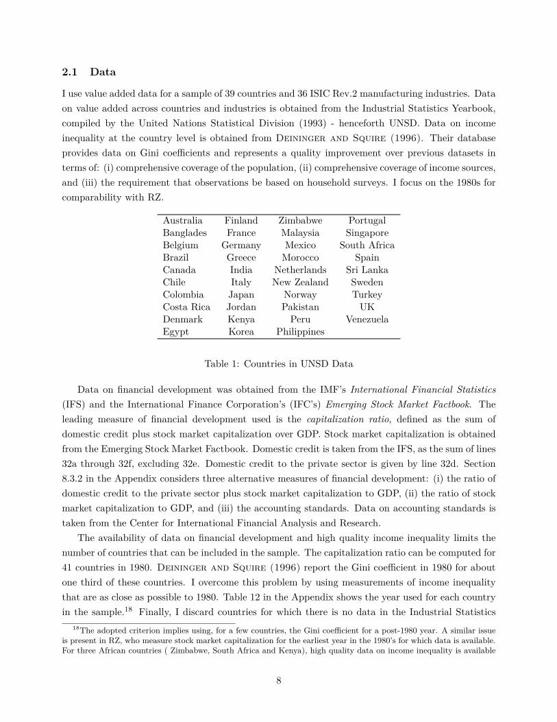
I use value added data for a sample of 39 countries and 36 ISIC Rev.2 manufacturing industries. Dataon value added across countries and industries is obtained from the Industrial Statistics Yearbook,compiled by the United Nations Statistical Division (1993) - henceforth UNSD. Data on incomeinequality at the country level is obtained from Deininger and Squire (1996). Their databaseprovides data on Gini coefficients and represents a quality improvement over previous datasets interms of: (i) comprehensive coverage of the population, (ii) comprehensive coverage of income sources,and (iii) the requirement that observations be based on household surveys. I focus on the 1980s forcomparability with RZ.

Australia Finland Zimbabwe PortugalBanglades France Malaysia SingaporeBelgium Germany Mexico South AfricaBrazil Greece Morocco SpainCanada India Netherlands Sri LankaChile Italy New Zealand SwedenColombia Japan Norway TurkeyCosta Rica Jordan Pakistan UKDenmark Kenya Peru VenezuelaEgypt Korea Philippines

Table 1: Countries in UNSD Data

Data on financial development was obtained from the IMF’s International Financial Statistics(IFS) and the International Finance Corporation’s (IFC’s) Emerging Stock Market Factbook. Theleading measure of financial development used is the capitalization ratio, defined as the sum ofdomestic credit plus stock market capitalization over GDP. Stock market capitalization is obtainedfrom the Emerging Stock Market Factbook. Domestic credit is taken from the IFS, as the sum of lines32a through 32f, excluding 32e. Domestic credit to the private sector is given by line 32d. Section8.3.2 in the Appendix considers three alternative measures of financial development: (i) the ratio ofdomestic credit to the private sector plus stock market capitalization to GDP, (ii) the ratio of stockmarket capitalization to GDP, and (iii) the accounting standards. Data on accounting standards istaken from the Center for International Financial Analysis and Research.

The availability of data on financial development and high quality income inequality limits thenumber of countries that can be included in the sample. The capitalization ratio can be computed for41 countries in 1980. Deininger and Squire (1996) report the Gini coefficient in 1980 for aboutone third of these countries. I overcome this problem by using measurements of income inequalitythat are as close as possible to 1980. Table 12 in the Appendix shows the year used for each countryin the sample.18 Finally, I discard countries for which there is no data in the Industrial Statistics

18The adopted criterion implies using, for a few countries, the Gini coefficient for a post-1980 year. A similar issueis present in RZ, who measure stock market capitalization for the earliest year in the 1980’s for which data is available.For three African countries ( Zimbabwe, South Africa and Kenya), high quality data on income inequality is available

8

Yearbook that is separated by at least 5 years during the 80s.19 The final sample consists of 39countries, which are listed in Table 1.20

Data on external financial dependence for 36 3-digit ISIC manufacturing sectors during the 1980sis taken from Rajan and Zingales (1998). They use firm-level data on publicly traded US firmsfrom Compustat (1994) and measure a firm’s dependence on external finance as the fraction of capitalexpenditures that is not financed with internal cashflows from operations. Table 13 in Section 8.2 ofthe Appendix lists the 36 sectors, in order of increasing external financial dependence.

2.2 A First Pass: Split-Sample Analysis

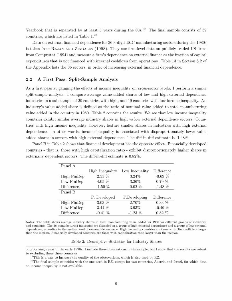
As a first pass at gauging the effects of income inequality on cross-sector levels, I perform a simplesplit-sample analysis. I compare average value added shares of low and high external dependenceindustries in a sub-sample of 20 countries with high, and 19 countries with low income inequality. Anindustry’s value added share is defined as the ratio of nominal value added to total manufacturingvalue added in the country in 1980. Table 2 contains the results. We see that low income inequalitycountries exhibit similar average industry shares in high vs low external dependence sectors. Coun-tries with high income inequality, however, feature smaller shares in industries with high externaldependence. In other words, income inequality is associated with disproportionately lower valueadded shares in sectors with high external dependence. The diff-in-diff estimate is -1.48%.

Panel B in Table 2 shows that financial development has the opposite effect. Financially developedcountries - that is, those with high capitalization ratio - exhibit disproportionately higher shares inexternally dependent sectors. The diff-in-diff estimate is 0.82%.

Panel AHigh Inequality Low Inequality Difference

High FinDep 2.55 % 3.24% -0.69 %Low FinDep 4.05 % 3.26% 0.79 %Difference -1.50 % -0.02 % -1.48 %Panel B

F. Developed F.Developing DifferenceHigh FinDep 3.03 % 2.70% 0.33 %Low FinDep 3.44 % 3.93% -0.49 %Difference -0.41 % -1.23 % 0.82 %

Notes: The table shows average industry shares in total manufacturing value added for 1980 for different groups of industriesand countries. The 36 manufacturing industries are classified in a group of high external dependence and a group of low externaldependence, according to the median level of external dependence. High inequality countries are those with Gini coefficient largerthan the median. Financially developed countries are those with capitalization ratio larger than the median.

Table 2: Descriptive Statistics for Industry Shares

only for single year in the early 1990s. I include these observations in the sample, but I show that the results are robustto excluding these three countries.

19This is a way to increase the quality of the observations, which is also used by RZ.20The final sample coincides with the one used in RZ, except for two countries, Austria and Israel, for which data

on income inequality is not available.

9

2.3 Cross-Country Analysis

I now study the effect of income inequality and financial development on relative value added at thecountry level. I define log relative value added in country k as lrvak ≡ log(vaHk)− log(vaLk), wherevaHk is nominal value added in sectors with external dependence higher than the median in countryk in 1980, and vaLk is similarly defined for industries with external financial dependence lower thanthe median. I estimate the following specification on the cross-section of countries:

lrvak = c+ β1λk + β2Gk + γXk + ε (1)

where λk is the capitalization ratio in 1980, Gk is the income Gini coefficient in 198021, and Xk is avector of country-level controls including the stock of human capital (defined as years of schooling inthe population over 25), per capita income, and indicators of the origin of the legal system (British,French, German, or Scandinavian).

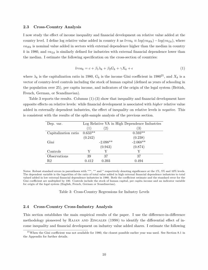
Table 3 reports the results. Columns (1)-(3) show that inequality and financial development haveopposite effects on relative levels: while financial development is associated with higher relative valueadded in externally dependent industries, the effect of inequality on relative levels is negative. Thisis consistent with the results of the split-sample analysis of the previous section.

Dep. var. Log Relative VA in High Dependence Industries(1) (2) (3)

Capitalization ratio 0.633** 0.593**(0.242) (0.238)

Gini -2.098** -2.068**(0.943) (0.874)

Controls Y Y YObservations 39 37 37R2 0.412 0.393 0.494

Notes: Robust standard errors in parentheses with ∗∗∗, ∗∗ and ∗ respectively denoting significance at the 1%, 5% and 10% levels.The dependent variable is the logarithm of the ratio of total value added in high external financial dependence industries to totalvalued added in low external financial dependence industries in 1980. Both the coefficient estimate and the standard error for theGini coefficient are multiplied by 100. Controls include the stock of human capital, per capita income and an indicator variablefor origin of the legal system (English, French, German or Scandinavian).

Table 3: Cross-Country Regressions for Industry Levels

2.4 Cross-Country Cross-Industry Analysis

This section establishes the main empirical results of the paper. I use the difference-in-differencemethodology pioneered by Rajan and Zingales (1998) to identify the differential effect of in-come inequality and financial development on industry value added shares. I estimate the following

21When the Gini coefficient was not available for 1980, the closest possible earlier year was used. See Section 8.1 inthe Appendix for further details.

10

specification:log(sjk) = c+ αj + αk + β1edjλk

+ β2edjGk + β3edjλkGk + εjk (2)

where sjk is industry j’s share of total value added in manufacturing in 1980 and edj is the levelof external financial dependence in industry j. This empirical model includes two double interac-tion terms and a triple interaction one. Since our interest lies on the interactions between financialdevelopment and inequality, a specification including all possible interactions between external de-pendence at the sector level and income inequality and financial development at the country level isnecessary. The advantage of this difference-in-difference approach comes from the inclusion of coun-try and sector fixed effects. I am thus able to address the issue of bias from omitted country-specificand industry-specific variables. Apart from these fixed effects, only RHS regressors that vary withboth industry and country are required.

To interpret the estimation of (2), it is useful to consider the difference in log value added sharesbetween a sector with high (H) and a sector with low (L) external dependence, log(sHk)− log(sLk).This log share differential is equal to log relative value added, as defined in Section 2.3. Thus,differencing equation (2) we have that:

∂lrvak∂Gk

= (β2 + β3λk) ∆ed, (3)

which means that relative value added is decreasing in the level of income inequality as long asβ2 + β3λk < 0. Note that (3) makes clear the presence of interaction effects: if β3 < 0, we have thatfinancial development strengthens the negative effect of income inequality on relative value added.Likewise, the effect of financial development on relative value added is given by

∂lrvak∂λk

= (β1 + β3Gk) ∆ed (4)

Financial development generates an increase in relative value added as long as β1 + β3Gk > 0.If additionally β3 < 0, an increase in income inequality weakens the positive effect of financialdevelopment on relative value added.

Table 4 contains the results of the estimation of (2). I find that industries with high reliance onexternal finance account for a lower share of total manufacturing value added in countries where thedistribution of income is more unequally distributed (see column (2)). Columns (3) and (4) showthat these results do not go away when both financial development and inequality terms are includedat the same time.22 Furthermore, I find that industries that are more dependent on external financeaccount for a relatively higher share of total manufacturing value added in more financially developedcountries.

22It should be noted that, in spite of the lack of significance of the double interaction term between inequalityand external financial dependence in column (4), the effect of inequality on relative shares is still negative, as thetriple interaction term is negative and significant. Also, it should be noted that, at the average level of inequality, thecoefficients of column (4) imply a positive effect of financial development on industry shares.

11

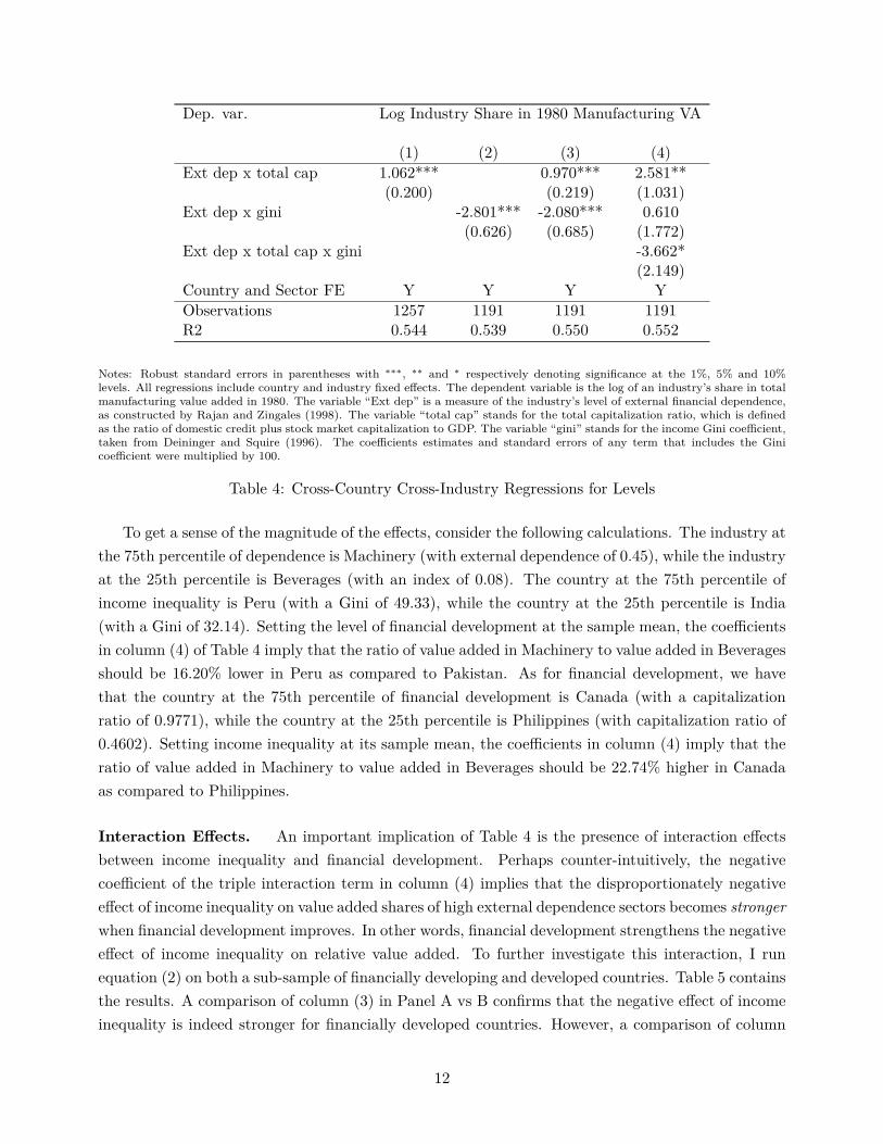
Dep. var. Log Industry Share in 1980 Manufacturing VA

(1) (2) (3) (4)Ext dep x total cap 1.062*** 0.970*** 2.581**

(0.200) (0.219) (1.031)Ext dep x gini -2.801*** -2.080*** 0.610

(0.626) (0.685) (1.772)Ext dep x total cap x gini -3.662*

(2.149)Country and Sector FE Y Y Y YObservations 1257 1191 1191 1191R2 0.544 0.539 0.550 0.552

Notes: Robust standard errors in parentheses with ∗∗∗, ∗∗ and ∗ respectively denoting significance at the 1%, 5% and 10%levels. All regressions include country and industry fixed effects. The dependent variable is the log of an industry’s share in totalmanufacturing value added in 1980. The variable “Ext dep” is a measure of the industry’s level of external financial dependence,as constructed by Rajan and Zingales (1998). The variable “total cap” stands for the total capitalization ratio, which is definedas the ratio of domestic credit plus stock market capitalization to GDP. The variable “gini” stands for the income Gini coefficient,taken from Deininger and Squire (1996). The coefficients estimates and standard errors of any term that includes the Ginicoefficient were multiplied by 100.

Table 4: Cross-Country Cross-Industry Regressions for Levels

To get a sense of the magnitude of the effects, consider the following calculations. The industry atthe 75th percentile of dependence is Machinery (with external dependence of 0.45), while the industryat the 25th percentile is Beverages (with an index of 0.08). The country at the 75th percentile ofincome inequality is Peru (with a Gini of 49.33), while the country at the 25th percentile is India(with a Gini of 32.14). Setting the level of financial development at the sample mean, the coefficientsin column (4) of Table 4 imply that the ratio of value added in Machinery to value added in Beveragesshould be 16.20% lower in Peru as compared to Pakistan. As for financial development, we havethat the country at the 75th percentile of financial development is Canada (with a capitalizationratio of 0.9771), while the country at the 25th percentile is Philippines (with capitalization ratio of0.4602). Setting income inequality at its sample mean, the coefficients in column (4) imply that theratio of value added in Machinery to value added in Beverages should be 22.74% higher in Canadaas compared to Philippines.

Interaction Effects. An important implication of Table 4 is the presence of interaction effectsbetween income inequality and financial development. Perhaps counter-intuitively, the negativecoefficient of the triple interaction term in column (4) implies that the disproportionately negativeeffect of income inequality on value added shares of high external dependence sectors becomes strongerwhen financial development improves. In other words, financial development strengthens the negativeeffect of income inequality on relative value added. To further investigate this interaction, I runequation (2) on both a sub-sample of financially developing and developed countries. Table 5 containsthe results. A comparison of column (3) in Panel A vs B confirms that the negative effect of incomeinequality is indeed stronger for financially developed countries. However, a comparison of column

12

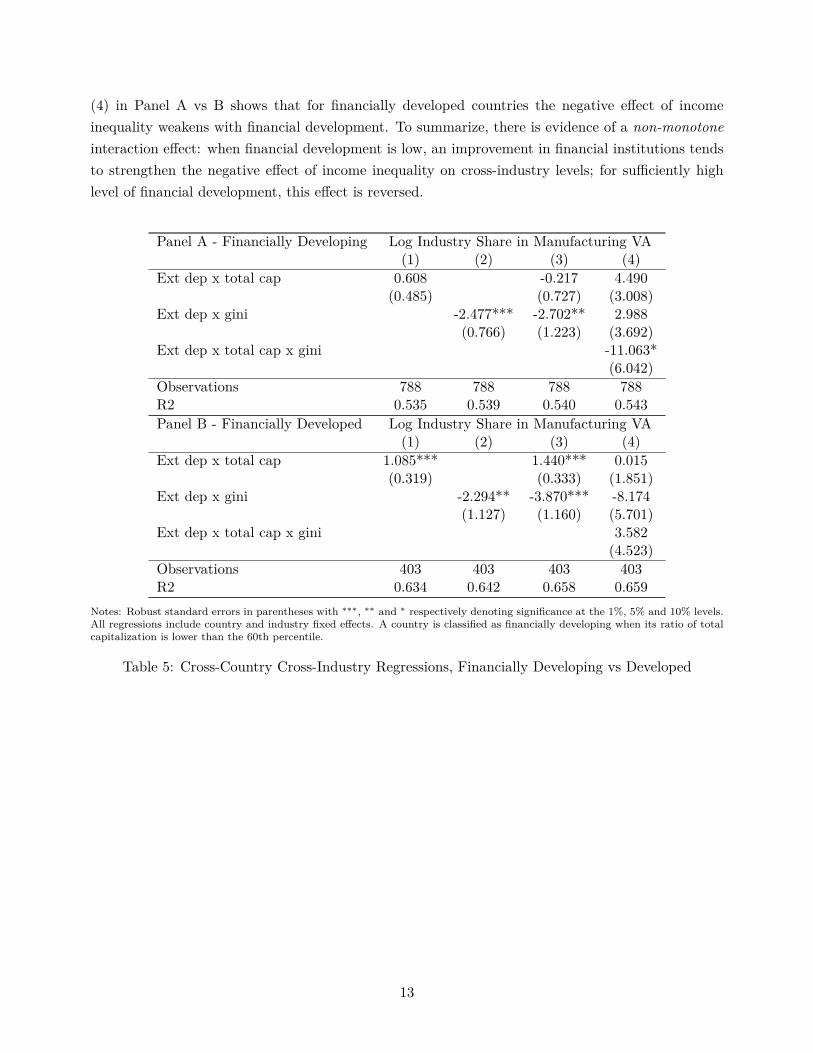
(4) in Panel A vs B shows that for financially developed countries the negative effect of incomeinequality weakens with financial development. To summarize, there is evidence of a non-monotoneinteraction effect: when financial development is low, an improvement in financial institutions tendsto strengthen the negative effect of income inequality on cross-industry levels; for sufficiently highlevel of financial development, this effect is reversed.

Panel A - Financially Developing Log Industry Share in Manufacturing VA(1) (2) (3) (4)

Ext dep x total cap 0.608 -0.217 4.490(0.485) (0.727) (3.008)

Ext dep x gini -2.477*** -2.702** 2.988(0.766) (1.223) (3.692)

Ext dep x total cap x gini -11.063*(6.042)

Observations 788 788 788 788R2 0.535 0.539 0.540 0.543Panel B - Financially Developed Log Industry Share in Manufacturing VA

(1) (2) (3) (4)Ext dep x total cap 1.085*** 1.440*** 0.015

(0.319) (0.333) (1.851)Ext dep x gini -2.294** -3.870*** -8.174

(1.127) (1.160) (5.701)Ext dep x total cap x gini 3.582

(4.523)Observations 403 403 403 403R2 0.634 0.642 0.658 0.659

Notes: Robust standard errors in parentheses with ∗∗∗, ∗∗ and ∗ respectively denoting significance at the 1%, 5% and 10% levels.All regressions include country and industry fixed effects. A country is classified as financially developing when its ratio of totalcapitalization is lower than the 60th percentile.

Table 5: Cross-Country Cross-Industry Regressions, Financially Developing vs Developed

13

3 The Model

The goal of this section is to provide a theory to account for the facts on income inequality andfinancial development documented in the previous section. I build the simplest theory that canaddress, qualitatively and quantitatively, the facts. To do so, I include the following core ingredientsin the theory. First, agents are heterogeneous in their wealth holdings, a feature that is essential tostudy the effects of wealth inequality.23 Second, there are two sectors in the economy. While several ofthe channels by which inequality affects economic development in the model would also be present ina one-sector economy, multiple sectors are needed to contrast the theory with findings of the previoussection. Third, agents face collateral constraints. This element is necessary to account for the effectsof financial development, and its interactions with income inequality, documented above. In themodel, collateral constraints imply that the distribution of wealth has an effect on the distributionof firm size. Fourth, there are decreasing returns to scale in production. This assumption guaranteesthat the distribution of firm size has an effect on the overall degree of production efficiency. Togetherwith collateral constraints, this element ensures that the distribution of wealth affects the productionside of the economy. Fifth, there are sector-specific fixed costs. The presence of fixed costs createsan extensive margin channel for inequality, as changes in the distribution of wealth affect the massof agents who can afford the fixed cost. Additionally, the difference in fixed costs across sectorsprovides a natural way to map the theory to the data. The sector with higher fixed cost turns out tobe the more externally dependent one. Sixth, there is occupational and sectoral choice. Without thisassumption, the distribution of wealth within the different sectors and occupations would becomea primitive of the model, and, due to cross-country data limitations, this would complicate thecalibration and model testing exercises.24

Finally, I consider a static model where the distribution of wealth is exogenously given. I do nottake a stand on the underlying determinant of wealth inequality - whether it is preferences for re-distribution (Alesina and Giuliano (2009)), geographic conditions (Engerman and Sokoloff(2002), Easterly (2007)) or heterogeneity in time discount factors (Krusell and Smith (1998),Krueger, Mitman, and Perri (2016)). In this sense, the approach of this paper is related to thestatic approach in development accounting (Caselli (2005)), which assumes an aggregate produc-tion function that maps factor endowments to income. The model presented below provides one suchproduction function where the entire distribution of capital holdings, and not just its mean, matters.

23In the baseline model, I abstract from heterogeneity in ability. Instead, I focus on redistributions of wealth amongagents of similar productivity. I do not study changes in the distribution of wealth across agents of different ability.Section 8.8 in the Appendix provides an extension of the model with heterogeneity in both wealth and ability.

24The assumption of occupational and sectoral choice implies that the country-wide distribution of wealth can berecovered from the country-wide distribution of income, which is observable for a wide range of countries - see Sections4 and 5 for details. Since data on income distribution at the sector/occupation level is typically not available for a widerange of countries, this assumption makes the calibration of the model possible, without the need of making furtherassumptions on the between-sector and within-sector distributions.

14

3.1 Environment

I consider an economy with two intermediate sectors (i = 1, 2) and one final good sector. The finalgood is both a consumption good and an input into the production of the intermediates. In turn,the intermediates are used for the production of the final good. The final good is assumed to be thenumeraire.

The economy is populated by a unit mass of producer-consumer agents who are endowed withphysical capital, or wealth, and labor. I assume that all agents are endowed with the same amountof labor (normalized to unity) and that wealth is the only dimension of heterogeneity among agents.I relax this assumption in Section 8.8 of the Appendix where I extend the model to incorporateheterogeneity in ability. I denote by G(ω) the distribution of initial wealth. Agents derive utilityfrom consumption of the final good.

At the beginning of the period, agents choose their occupation: they can work for a wage w,or operate a business in intermediate good sector 1 or 2.25 For simplicity, it is assumed that theycannot engage in production of the final good. To start a firm in intermediate sector i, agents mustpay a sector-specific fixed cost of fi units of capital. The intermediate sectors are assumed to differin their fixed cost requirement, with f2 > f1. As will be clear below, this will imply that sector 2 isthe more externally dependent sector. After paying the fixed cost, the agents produce according tothe following technology:

Ai(kαl1−α)ν (5)

where k denotes capital (or units of the final good), l denotes labor, ν is the share of payment goingto the variable factors - that is, the span-of-control parameter (Lucas (1978)) -, α is the share ofthis payment going to capital, and Ai is sector-level productivity. It is assumed that α, ν ∈ (0, 1),which means that intermediate producers are subject to diminishing returns to scale. Note that whilethe factor elasticities in (5) are identical across sectors, sector 2 is in effect more capital intensivedue to its higher fixed cost.

Production of the final good is done by a set of competitive firms, who have access to a constantreturns to scale technology, [

γYε−1ε

1 + (1− γ)Yε−1ε

2

] εε−1

where γ ∈ (0, 1), ε ∈ [0,∞) and Yi denotes quantity of intermediate input i. Note that productionof the final good does not require a fixed cost. Final good firms start with no wealth and earn zeroprofits.

After agents have chosen their occupation, a market for capital rental meets where capital is lentat rate r. As is common in the literature (Buera, Kaboski, and Shin (2011),Midrigan and Xu(2014),Evans and Jovanovic (1989)), it is assumed that capital loans are due at the end of theperiod. The crucial assumption is that trade in the capital market is subject to a friction, by whichthe amount of borrowing is limited by the entrepreneur’s net worth. I assume that agents can borrowup to a fraction of their wealth. More precisely, an agent with wealth ω is able to borrow a total

25Agents can at most have one occupation. That is, an agent cannot both run a firm and be a worker.

15

of (λ − 1)ω, where λ ≥ 1 is a parameter that captures the degree of financial development in theeconomy. This specification of the borrowing constraint is widely used in literature (Banerjee andNewman (2003), Buera and Shin (2013)), and is chosen for tractability reasons. A higher valueof λ is associated with better financial markets, with λ = 1 corresponding to the absence of creditand λ =∞ corresponding to perfect capital markets.26

3.2 Equilibrium

In this section, I study the behavior of entrepreneurs and final good firms. I then define and charac-terize the equilibrium.

Problem of Entrepreneurs. Entrepreneurs’ occupational and production decisions are as follows.First, they must decide whether to work for a wage, or engage in production of intermediate goods.If they become entrepreneurs, they need to choose a sector in which to operate, how much output toproduce and which combination of inputs to employ. Assuming, without loss of generality, that allcapital is borrowed, the production problem of agent ω in sector i is:

πi (ω) = maxk,l

piAi(kαl1−α)ν − wl − (r + δ) (k + fi) s.t. k + fi ≤ λω (6)

where pi denotes the price of intermediate good i and w denotes the wage rate. Note that I haveassumed that the fixed cost and working capital both depreciate at the same rate. The unconstrainedsolution to this problem is given by

kui =(piAiν

(1− αw

)ν(1−α) ( α

r + δ

)1−ν(1−α)) 1

1−ν

(7)

lui =(piAiν

(1− αw

)1−αν ( α

r + δ

)αν) 11−ν

(8)

with associated unconstrained profits

πui = (1− ν)(piAiν

ν(

α

r + δ

)αν (1− αw

)(1−α)ν) 1

1−ν

− (r + δ)fi (9)

The solution to the constrained problem is given by

ki (ω) = min {max {λω − fi, 0} , kui } (10)

li (ω) =(piAiν(1− α)

w

) 11−ν(1−α)

ki (ω)αν

1−(1−α)ν (11)

26For simplicity, I assume that final good firms are not subject to the financial friction.

16

Agents with wealth below fi/λ cannot enter into sector i. This introduces a non-convexity that willplay an important role in the analysis. Finally, profits after entry into sector i are

πi (ω) =( 1

(1− α)ν − 1)(

piAi(1− α)νw(1−α)ν

) 11−(1−α)ν

ki (ω)αν

1−(1−α)ν − (r + δ) (ki (ω) + f) (12)

Each entrepreneur sorts into the occupation/sector that is most profitable to her, with resultingprofits before entry of π(ω) = max{w, π1(ω), π2(ω)}. Output is given by

yi(ω) = A( 1wpiA(1− α)ν)

(1−α)ν1−(1−α)ν ki(ω)

αν1−(1−α)ν

Final good producer problem. Final good producers, who are not subject to financial frictions,solve the following problem:

maxY1,Y2

[γY

ε−1ε

1 + (1− γ)Yε−1ε

2

] εε−1− p1Y1 − p2Y2

First order conditions imply:

γ

1− γ

(Y1Y2

)− 1ε

= p1p2

(13)

I normalize the price of the final good to unity which, together with free entry into the final goodsector, implies: [

γεp1−ε1 + (1− γ)ε p1−ε

2

] 11−ε = 1

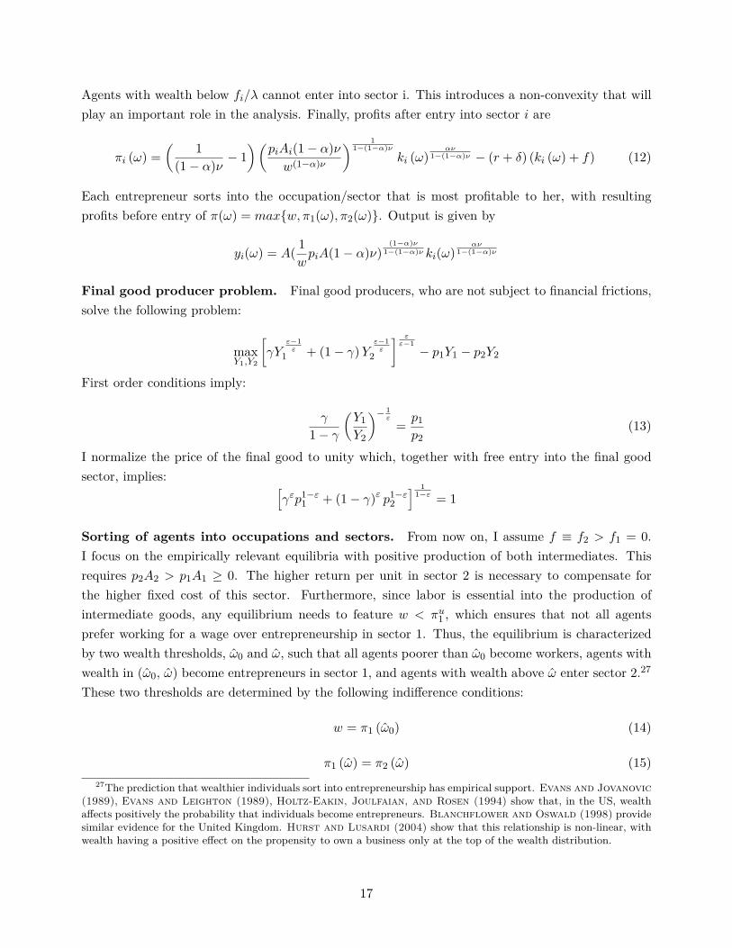
Sorting of agents into occupations and sectors. From now on, I assume f ≡ f2 > f1 = 0.I focus on the empirically relevant equilibria with positive production of both intermediates. Thisrequires p2A2 > p1A1 ≥ 0. The higher return per unit in sector 2 is necessary to compensate forthe higher fixed cost of this sector. Furthermore, since labor is essential into the production ofintermediate goods, any equilibrium needs to feature w < πu1 , which ensures that not all agentsprefer working for a wage over entrepreneurship in sector 1. Thus, the equilibrium is characterizedby two wealth thresholds, ω0 and ω, such that all agents poorer than ω0 become workers, agents withwealth in (ω0, ω) become entrepreneurs in sector 1, and agents with wealth above ω enter sector 2.27

These two thresholds are determined by the following indifference conditions:

w = π1 (ω0) (14)

π1 (ω) = π2 (ω) (15)27The prediction that wealthier individuals sort into entrepreneurship has empirical support. Evans and Jovanovic

(1989), Evans and Leighton (1989), Holtz-Eakin, Joulfaian, and Rosen (1994) show that, in the US, wealthaffects positively the probability that individuals become entrepreneurs. Blanchflower and Oswald (1998) providesimilar evidence for the United Kingdom. Hurst and Lusardi (2004) show that this relationship is non-linear, withwealth having a positive effect on the propensity to own a business only at the top of the wealth distribution.

17

For given prices, Figure 1 shows the returns to each occupation as a function of wealth.28 Thepresence of a higher fixed cost in sector 2 implies that wealthy individuals have a comparativeadvantage in this sector. Intuitively, the decision of entering sector 2 instead of sector 1 is equivalentto the payment of a fixed cost in exchange for a higher (effective) price per unit. Such decision isprofitable for a sufficiently large volume of production, which, under borrowing constraints, happensfor wealthy enough entrepreneurs. It is important to note that agents with sufficiently low wealth(ω < f/λ) are not able to enter sector 2, so that their occupational choice is restricted to workingfor a wage vs entrepreneurship in sector 1.

w

��� ��

-(r+δ)f ω

π1

π2

Figure 1: Occupation and Sector Sorting

Equilibrium Definition. Given a distribution of wealth G(ω), an equilibrium with positive pro-duction of both intermediates consists of prices (p1, p2, r, w) and wealth thresholds (ω0, ω) such that:

1. Marginal agents are indifferent:w = π1 (ω0)

π1 (ω) = π2 (ω)

2. Capital market clears:∫ ω

ω0k1 (ω) dG (ω) +

∫ ∞ω

(k2 (ω) + f)dG (ω) = E [ω] (16)28Note that for wealth values below f/λ profits in sector 2 are not defined.

18

3. Labor market clears: ∫ ω

ω0l1 (ω) dG (ω) +

∫ ∞ω

l2 (ω) dG (ω) = G(ω0) (17)

4. Final good producers’ optimality:∫ ω

ω0A1k1 (ω)αν l1 (ω)(1−α)ν dG (ω) =

(γ

1− γp2p1

)ε ∫ ∞ω

A2k2 (ω)αν l2 (ω)(1−α)ν dG (ω) (18)

5. Zero profits in final good: [γεp1−ε

1 + (1− γ)ε p1−ε2

] 11−ε = 1 (19)

The equilibrium prices and wealth thresholds completely characterize production in the economy,for a given distribution of wealth. Implicit in this definition is the extensive margin constraint thatω ≥ f/λ.29 This constraint requires that the mass of agents allocated to sector 2 in equilibrium doesnot exceed the mass of agents that are wealthier than the effective fixed cost, f/λ.30

3.3 Effects of Wealth Inequality

The main purpose of this paper is to study the effects of increased wealth inequality on macroeconomicaggregates. In the model, the presence of financial frictions implies that the distribution of wealthaffects the allocation of productive resources, and thus has an impact on aggregate production. Butwhat is the nature of this link? Does a more unequal distribution of wealth lead to higher or lowerproduction efficiency?

To think about this question, it is useful to consider three channels through which higher wealthinequality affects the economy. Consider a simple example in which a unit of capital is redistributedfrom a poor and constrained agent to a wealthier, not necessarily constrained agent. First, there isa decreasing returns channel. Since the wealthy agent is operating at a bigger scale, her marginalproduct of capital is lower than that of the poor-constrained agent. Thus, a poor-to-rich redistributionof capital will decrease output.31 To see this more formally, consider average output in sector 1:

1G(ω0)−G(ω)

∫ ω

ω0y1(ω)dG(ω) = 1

G(ω0)−G(ω)

∫ ω

ω0A( 1wp1A(1− α)ν)

(1−α)ν1−(1−α)ν k1(ω)

αν1−(1−α)ν dG(ω)

Since k1(ω) is a concave function of wealth, and α, ν ∈ (0, 1), output y1(ω) is also a concave function ofwealth. Thus, for given prices and wealth thresholds, any mean preserving spread to the distributionof wealth of agents in sector 1 will reduce average output in this sector.32 Note that this is a partial

29This constraint is implicit in condition (1) of the equilibrium definition, as π2 (ω) is not defined for ω < f/λ.30In an equilibrium with positive production of both intermediate goods, this constraint turns out to not bind (i.e.

ω > f/λ). This follows directly from the fact that π1 (f/λ) > 0 > −(r+ δ)f = π2 (f/λ). Intuitively, it is never sociallyoptimal to assign the agent with wealth exactly equal to f/λ to sector 2, since he would produce no output and incurin a cost of f units of capital.

31For simplicity, I focus on the case where both entrepreneurs produce in the same sector.32That is, a mean preserving spread to G(ω)

G(ω0)−G(ω) .

19

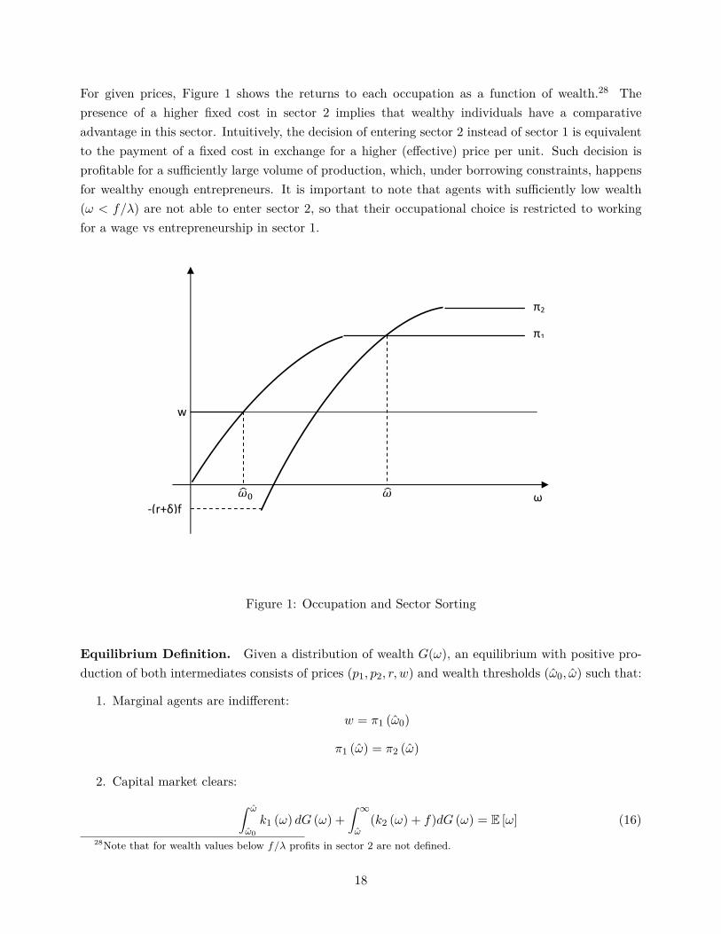
equilibrium effect, as prices and wealth thresholds are kept constant.Second, there is a capital demand channel. If the two agents are constrained entrepreneurs, the

linearity of the borrowing constraint implies that a redistribution of wealth has no effect on capitaldemand. If the wealthier agent has reached the optimal scale and the poorer has not, then a poor-to-rich redistribution of wealth between the two entrepreneurs decreases capital demand. This isbecause the richer agent has no use for the extra unit of capital other than lending, but the pooragent is at her maximum borrowing capacity. Figure 2 depicts the capital demand channel. To seethis effect more formally, consider total capital demand for the case in which all agents in sector 1are constrained (which happens when ku1/λ ≥ ω),

∫∞ω0h (ω) dG (ω), where h(ω) = min {λω, ku2 + f}

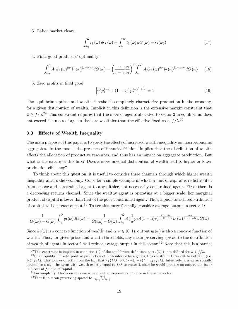
is capital demand of agent ω irrespective of her sector. As h(ω) is concave, any mean preservingspread to the distribution of wealth among entrepreneurs reduces total capital demand.33 However,we can also have a situation where the wealthier agent is constrained while the poorer one is not.Figure 3 depicts this situation. In this case, a poor-to-rich redistribution of wealth between the twoagents increases capital demand. Formally, the capital demand function is not globally concave and amean preserving spread can result in higher aggregate capital demand. Finally, if the relatively pooragent is a worker while the wealthier one is a constrained entrepreneur, aggregate capital demandalso increases.

��� + �

��� + �

�

ωP ω'P ω'R �� ωR ω

Figure 2: Wealth Inequality and the Capital Demand Channel33A reduction in capital demand, and the associated reduction in labor demand, harm the economy by depressing

the interest rate and the wage. The depressed interest rate and wage lead to an excessive amount of entrepreneurship,as well as to an inefficiently high scale of production units. See Section 4 for more details.

20

���

���

�

��� + �

��� + �

�

ωP ω'P ω'R � ωR ω

Figure 3: Wealth Inequality and the Capital Demand Channel, II

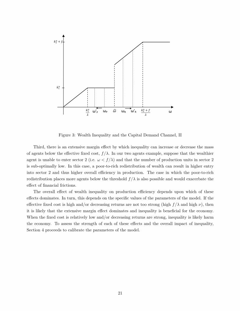
Third, there is an extensive margin effect by which inequality can increase or decrease the massof agents below the effective fixed cost, f/λ. In our two agents example, suppose that the wealthieragent is unable to enter sector 2 (i.e. ω < f/λ) and that the number of production units in sector 2is sub-optimally low. In this case, a poor-to-rich redistribution of wealth can result in higher entryinto sector 2 and thus higher overall efficiency in production. The case in which the poor-to-richredistribution places more agents below the threshold f/λ is also possible and would exacerbate theeffect of financial frictions.

The overall effect of wealth inequality on production efficiency depends upon which of theseeffects dominates. In turn, this depends on the specific values of the parameters of the model. If theeffective fixed cost is high and/or decreasing returns are not too strong (high f/λ and high ν), thenit is likely that the extensive margin effect dominates and inequality is beneficial for the economy.When the fixed cost is relatively low and/or decreasing returns are strong, inequality is likely harmthe economy. To assess the strength of each of these effects and the overall impact of inequality,Section 4 proceeds to calibrate the parameters of the model.

21

4 Calibration

In this section, I calibrate the technology parameters of the model to match several key momentsof the US economy. I use the US to identify the technology parameters because this country wasused to construct the sector-level measure of external financial dependence used in Section 2.34 Tocalibrate the technological parameters, I need to also calibrate the parameters of the distribution ofwealth and the quality of financial institutions in the US. When studying the effects of inequalityand financial development in the next two sections, I do not use the financial and wealth distributionparameters estimated in this section, but rather calibrate these parameters to the sample of countriesused to establish the facts in Section 2. In short, I identify the technological parameters from theUS and the non-technological parameters from the countries in the sample.

Parametrization of Wealth Distribution. I assume that wealth is Pareto distributed:

G(ω) = 1− (ωminω

)θ for ω ≥ ωmin

where θ > 1 is the shape parameter and ωmin is the scale parameter. This assumption is made fortwo reasons. First, this distribution turns out to be a good approximation for the upper tail of thewealth distribution (see Pareto (1897), Klass et al. (2006)). In Section 8.5 of the Appendix Iprovide evidence for this statement using Survey of Consumer Finances data for the US. Second, thePareto distribution is conveniently parametrized to study changes in inequality. The scale parametercontrols the average level of wealth, which is equal to: E [ω] = θ/(θ − 1)ωmin. The shape parametercontrols the degree of wealth inequality in the economy. Specifically, a lower value of θ generatesa uniform decrease in the Lorenz curve - that is, it generates a new distribution of wealth that isLorenz dominated. This increase in wealth inequality is fully captured by the wealth Gini coefficient,which is given by:

Gini = 12θ − 1

Calibration Strategy. The model has 8 technological parameters (α, ν,A1, A2, f, γ, ε, δ), 1 pa-rameter characterizing the quality of financial institutions (λ), and 2 parameters characterizing thedistribution of wealth (ωmin,θ). I take the annual depreciation rate to be δ = 0.06, a standard valuein the literature. I assume throughout the paper that there are no productivity differences acrosssectors, A1 = A2 = A, and I normalize this parameter to unity without loss of generality.35 I calibratethe remaining parameters to match salient moments of the US economy in the 1980s.

I start by calibrating the wealth distribution parameters (ωmin,θ) to match the mean and theGini coefficient of the US wealth distribution. I then estimate the elasticity of substitution betweenthe two intermediate sectors, ε, from a time series regression of relative values on relative quantities

34Note also that I have not included the US in the sample of countries used to establish the cross-sector facts ofSection 2.

35This assumption, which allows me to fully focus on differences in capital intensity across sectors, has been madeby other papers in the literature - see e.g. Buera, Kaboski, and Shin (2011) who assume the distribution of talentto be symmetric across sectors.

22

for the US. I then calibrate the remaining 5 technological parameters (γ, α, ν, f ,A) and the qualityof financial markets parameter (λ) to match the following 6 moments of the US economy in 1980: (i)the share of payments to capital in manufacturing GDP, (ii) the share of high externally dependentsectors in total manufacturing value added, (iii) relative capital per workers across sectors, (iv) theincome Gini coefficient, (v) the ratio of external finance to GDP. While these 5 parameters aresimultaneously chosen to match the 5 moments, it can be helpful to associate one parameter to eachmoment.36

As is typical in calibrations of the neo-classical growth model, we can think of α as controllingthe share of payments to capital in manufacturing GDP,

rE [ω] /Y (20)

It should be noted that, since the model has borrowing constraints and fixed costs, the share ofpayments to capital will not be exactly given by α, as in the frictionless model without fixed costs.In particular, the capital share can be lower than the value of α.

Consider now moment (ii). Since the intermediate goods are produced with only capital and labor,and do not require any further intermediate goods, we can interpret p2Y2 as value added in the highexternal dependence sector. We can think of 1−γ as controlling the share of the externally dependentsector in manufacturing GDP, p2Y2/Y . This is exactly true for the case in which technology in thefinal good sector is Cobb-Douglas - that is, ε = 1.

The third moment, relative capital per worker across sectors, identifies the fixed cost in the highexternal dependence sector, f . If the fixed cost was zero, the model would predict that capitalintensities should be equalized across sectors. A positive fixed cost makes sector 2 more capitalintensive, in the sense that (k2 + f)/l2 > (k1/l1). In partial equilibrium, a higher fixed cost triviallyincreases the relative capital labor ratio. In general equilibrium, however, prices and thresholdschange so that a higher fixed cost may have a non-monotone effect on relative capital intensity acrosssectors.37 At the calibrated parameters, this relationship is increasing.

36Moments (i) and (iii) are both related to the degree of capital intensity in production. Moment (i) affects bothsectors equally, while moment (iii) is included to get at the difference in capital intensity across sectors.

37For given prices, a higher fixed cost tends to increase capital demand, as unconstrained producers in sector 2will demand the same amount of working capital and a higher amount of capital for the fixed cost. Note that theconstrained agents in sector 2 demand the same amount of capital, as k2 + f = λω. However, these agents will use lessworking capital, k2, when the fixed cost is higher, so that labor demand falls. These effects tend to increase the interestrate and decrease the wage. The higher fixed cost has a negative direct effect on sector 2 profits, so that some agentsflow to sector 1. This tends to increase p2 and decrease p1. A constrained agent in sector i produces at the followingcapital to labor ratio - including fixed costs:

(λω)1−ν

1−(1−α)ν ( w

p2A(1 − α)ν ))1

1−(1−α)ν

Since p2 increases and p1 decreases, the capital labor ratio of constrained agents tends to decrease by more in sector 2.However, wealth thresholds also change: ω increases, so that sector 2 firms are larger on average - this tends to increasethe capital labor ratio in sector 2. At the same time, ω0 also increases. Thus, the average size of firms in sector 1 canmove in either direction. As for unconstrained agents, the increase in the relative price of capital tends to decrease k/lby same proportion in both sectors - in fact, unconstrained k/l ratios are equalized across sectors. But sector 2 agentshave a higher fixed costs, which tends to increase their unconstrained total capital labor ratio.

23

The span of control parameter, ν, is chosen to generate a realistic level of inequality in thedistribution of income. In other words, the model generates a mapping between the exogenouswealth distribution and the endogenous income distribution, and this mapping is crucially affectedby ν. To see this, note that agent ω’s income is given by

i(ω) = rω +max {w, π1 (ω) , π2 (ω)} (21)

For given prices, a higher ν leads to a steeper profit function πi(ω) in both sectors. To see this, notethat the profit function becomes a less concave function of wealth when ν is higher - see equation(12).38 Furthermore, an increase in ν leads to a higher interest rate, which also tends to increaseincome inequality. Finally, an increase in ν leads to a lower wage and a higher mass of workers, sothat income inequality is further increased.

The parameter governing the quality of financial institutions, λ, is chosen so that the modelgenerates an external finance to GDP ratio similar to that of the US in 1980. A higher λ naturallyleads to more borrowing, as poor-constrained agents expand their demand for capital.

Distribution of Wealth in the US. The assumption that wealth is Pareto distributed impliesthat only two moments of the US distribution of wealth are required for its calibration: average wealthand the wealth Gini coefficient. The latter moment allows me to identify the shape parameter, θ,and the former moment then pins down the scale parameter, ωmin. I use data from the 1983 Surveyof Consumer Finances (SCF) to characterize the distribution of wealth in the US. Because householdwealth is highly skewed, the upper tail of the distribution is often underrepresented in survey data.The advantage of the SCF data is that it provides a high-income supplement, which is taken fromthe Internal Revenue Service’s Statistics of Income data.39 Table 6 shows values for average wealthand the wealth Gini coefficient for the entire population of US households. These values implyθUS = 1.1412 and ωUSmin = $14, 813.88.

Average Wealth Wealth GiniAll US households $119,724 77.98

Notes: Data from the US Survey of Consumer Finances for 1983. Both the normal and the high income sample are included.Wealth (net worth) is given by variable B3324, which is defined as gross assets excluding pensions plus total net present value ofpensions minus total debt (B3305 + B3316 - B3320).

Table 6: Moments of Wealth Distribution, US 198338Consider revenue net of labor costs, that is, the first term of the profit function for a constrained entrepreneur:(

1(1 − α)ν − 1

)(piAi(1 − α)νw(1−α)ν

) 11−(1−α)ν

(λω)αν

1−(1−α)ν

It is easy to see that the rate of growth of this term with respect to wealth depends on the exponent αν1−(1−α)ν , which

is increasing in ν.39See Wolff (1999) for a comparison among 3 household surveys which report wealth: the SCF, the Bureau of the

Census’ Survey of Income and Program Participation, and the Institute for Social Research’s Panel Survey of IncomeDynamics.

24

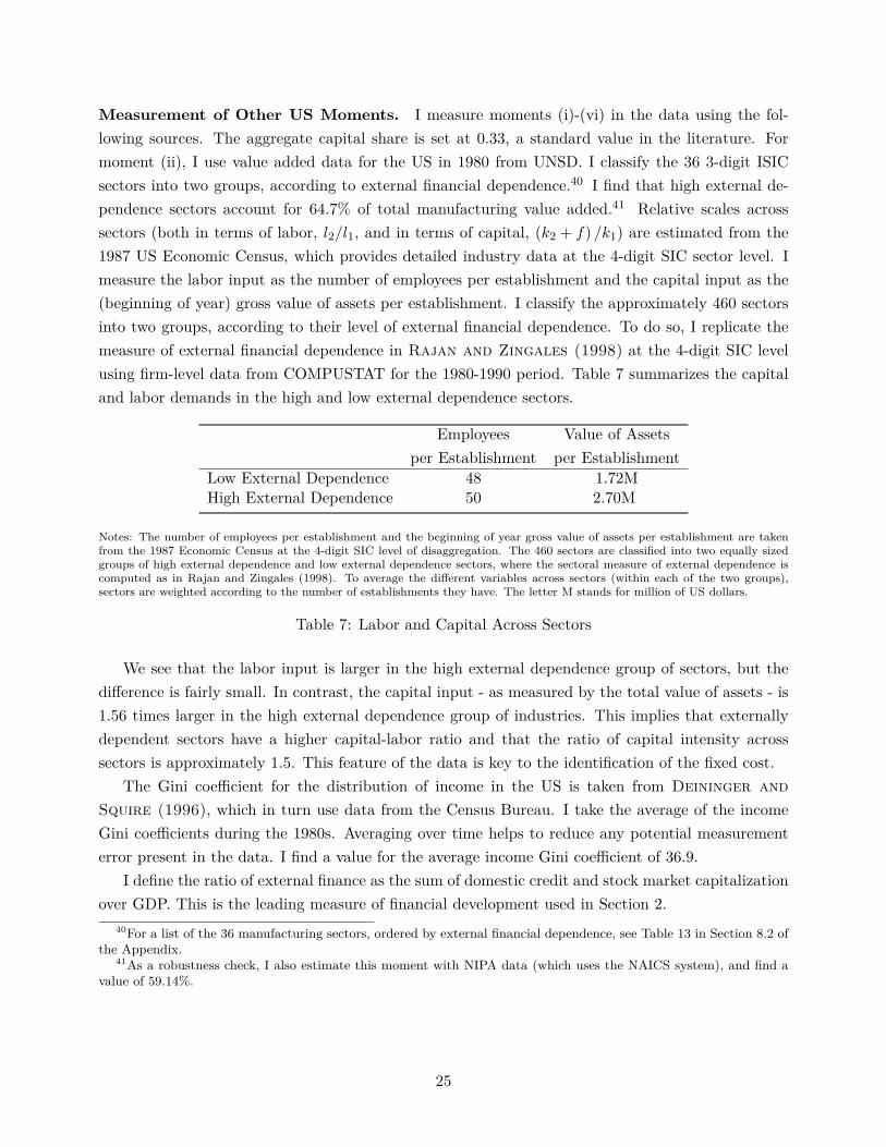
Measurement of Other US Moments. I measure moments (i)-(vi) in the data using the fol-lowing sources. The aggregate capital share is set at 0.33, a standard value in the literature. Formoment (ii), I use value added data for the US in 1980 from UNSD. I classify the 36 3-digit ISICsectors into two groups, according to external financial dependence.40 I find that high external de-pendence sectors account for 64.7% of total manufacturing value added.41 Relative scales acrosssectors (both in terms of labor, l2/l1, and in terms of capital, (k2 + f) /k1) are estimated from the1987 US Economic Census, which provides detailed industry data at the 4-digit SIC sector level. Imeasure the labor input as the number of employees per establishment and the capital input as the(beginning of year) gross value of assets per establishment. I classify the approximately 460 sectorsinto two groups, according to their level of external financial dependence. To do so, I replicate themeasure of external financial dependence in Rajan and Zingales (1998) at the 4-digit SIC levelusing firm-level data from COMPUSTAT for the 1980-1990 period. Table 7 summarizes the capitaland labor demands in the high and low external dependence sectors.

Employees Value of Assetsper Establishment per Establishment

Low External Dependence 48 1.72MHigh External Dependence 50 2.70M

Notes: The number of employees per establishment and the beginning of year gross value of assets per establishment are takenfrom the 1987 Economic Census at the 4-digit SIC level of disaggregation. The 460 sectors are classified into two equally sizedgroups of high external dependence and low external dependence sectors, where the sectoral measure of external dependence iscomputed as in Rajan and Zingales (1998). To average the different variables across sectors (within each of the two groups),sectors are weighted according to the number of establishments they have. The letter M stands for million of US dollars.

Table 7: Labor and Capital Across Sectors

We see that the labor input is larger in the high external dependence group of sectors, but thedifference is fairly small. In contrast, the capital input - as measured by the total value of assets - is1.56 times larger in the high external dependence group of industries. This implies that externallydependent sectors have a higher capital-labor ratio and that the ratio of capital intensity acrosssectors is approximately 1.5. This feature of the data is key to the identification of the fixed cost.

The Gini coefficient for the distribution of income in the US is taken from Deininger andSquire (1996), which in turn use data from the Census Bureau. I take the average of the incomeGini coefficients during the 1980s. Averaging over time helps to reduce any potential measurementerror present in the data. I find a value for the average income Gini coefficient of 36.9.

I define the ratio of external finance as the sum of domestic credit and stock market capitalizationover GDP. This is the leading measure of financial development used in Section 2.

40For a list of the 36 manufacturing sectors, ordered by external financial dependence, see Table 13 in Section 8.2 ofthe Appendix.

41As a robustness check, I also estimate this moment with NIPA data (which uses the NAICS system), and find avalue of 59.14%.

25

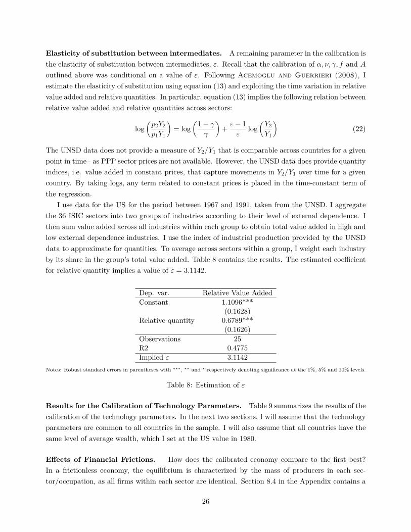
Elasticity of substitution between intermediates. A remaining parameter in the calibration isthe elasticity of substitution between intermediates, ε. Recall that the calibration of α, ν, γ, f and Aoutlined above was conditional on a value of ε. Following Acemoglu and Guerrieri (2008), Iestimate the elasticity of substitution using equation (13) and exploiting the time variation in relativevalue added and relative quantities. In particular, equation (13) implies the following relation betweenrelative value added and relative quantities across sectors:

log(p2Y2p1Y1

)= log

(1− γγ

)+ ε− 1

εlog

(Y2Y1

)(22)

The UNSD data does not provide a measure of Y2/Y1 that is comparable across countries for a givenpoint in time - as PPP sector prices are not available. However, the UNSD data does provide quantityindices, i.e. value added in constant prices, that capture movements in Y2/Y1 over time for a givencountry. By taking logs, any term related to constant prices is placed in the time-constant term ofthe regression.

I use data for the US for the period between 1967 and 1991, taken from the UNSD. I aggregatethe 36 ISIC sectors into two groups of industries according to their level of external dependence. Ithen sum value added across all industries within each group to obtain total value added in high andlow external dependence industries. I use the index of industrial production provided by the UNSDdata to approximate for quantities. To average across sectors within a group, I weight each industryby its share in the group’s total value added. Table 8 contains the results. The estimated coefficientfor relative quantity implies a value of ε = 3.1142.

Dep. var. Relative Value AddedConstant 1.1096***

(0.1628)Relative quantity 0.6789***

(0.1626)Observations 25R2 0.4775Implied ε 3.1142

Notes: Robust standard errors in parentheses with ∗∗∗, ∗∗ and ∗ respectively denoting significance at the 1%, 5% and 10% levels.

Table 8: Estimation of ε

Results for the Calibration of Technology Parameters. Table 9 summarizes the results of thecalibration of the technology parameters. In the next two sections, I will assume that the technologyparameters are common to all countries in the sample. I will also assume that all countries have thesame level of average wealth, which I set at the US value in 1980.

Effects of Financial Frictions. How does the calibrated economy compare to the first best?In a frictionless economy, the equilibrium is characterized by the mass of producers in each sec-tor/occupation, as all firms within each sector are identical. Section 8.4 in the Appendix contains a

26

Target Moment Data ParameterShare of Ext.Dep. Sectors in Manufacturing VA 0.647 γ= 0.4262Share of Capital in Manufacturing GDP 0.33 α = 0.5855Relative Capital Intensity in Ext.Dep. Sectors 1.50 f = $55,280Income Gini 35.2 ν =0.7153External Finance to GDP ratio 1.9624 λ = 3.0790

Notes: “Ext. Dep.” stands for externally dependent sectors. In the data, the 36 manufacturing sectors are classified into twogroups according to their level of external financial dependence, as measured by Rajan and Zingales (1998).

Table 9: Calibration of Technology Parameters

definition of the equilibrium in the first best economy. Table 10 shows selected equilibrium outcomesfor the calibrated US economy and the first best. Both economies share the same technology and dis-tribution of wealth parameters. By depressing capital and therefore labor demand, financial frictionstend to depress both the interest and the wage. The economy shifts its production pattern towardsthe less capital intensive sector. The depressed wage and interest rate lead to higher profits and thisresults in an excessive amount of entrepreneurship in the economy with frictions. The presence of afixed cost, together with financial frictions, results in too many firms in sector 1 and too few in sector2. Firms in sector 1 are on average too small relative to the first best size, while firms in sector 2 areon average too large. This distortion in firm size follows from the combination of the different priceeffects. The depressed interest rate and wage induce firms in both sectors to choose a higher scale.In sector 2, the higher price reinforces the increase in scale. In sector 1, the effect of the lower pricetends to dominate the interest rate and wage effect, and average scale is lower.

Calibrated First BestInterest Rate 0.0401 0.0876Wage $19,813 $19,517Price 1 0.4640 0.4822Price 2 0.5421 0.5326Mass Workers 0.5382 0.5649Mass Sector 1 0.2564 0.1781Mass Sector 2 0.2054 0.2570GDP $35,970 $37,188Average Capital Sector 1 $124,502 $194,514Average Capital Sector 2 $372,215 $275,834Rel. Output Sector 2 1.5763 1.8522

Notes: The table shows equilibrium outcomes for both the model with frictions calibrated to the US and the first best economy.For both economies, the technology parameters are set according to Table 9 and the wealth distribution is calibrated to the USas described in the previous section.

Table 10: Calibrated Economy vs First Best

Wealth Inequality - Income Inequality Mapping. In the next sections, I study the effectsof mean-preserving variation in wealth inequality on the economy. Since wealth inequality is not

27

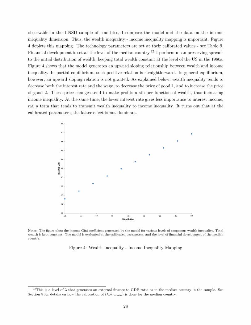
observable in the UNSD sample of countries, I compare the model and the data on the incomeinequality dimension. Thus, the wealth inequality - income inequality mapping is important. Figure4 depicts this mapping. The technology parameters are set at their calibrated values - see Table 9.Financial development is set at the level of the median country.42 I perform mean preserving spreadsto the initial distribution of wealth, keeping total wealth constant at the level of the US in the 1980s.Figure 4 shows that the model generates an upward sloping relationship between wealth and incomeinequality. In partial equilibrium, such positive relation is straightforward. In general equilibrium,however, an upward sloping relation is not granted. As explained below, wealth inequality tends todecrease both the interest rate and the wage, to decrease the price of good 1, and to increase the priceof good 2. These price changes tend to make profits a steeper function of wealth, thus increasingincome inequality. At the same time, the lower interest rate gives less importance to interest income,rω, a term that tends to transmit wealth inequality to income inequality. It turns out that at thecalibrated parameters, the latter effect is not dominant.

30

32

34

36

38

40

42

Inco

me

Gin

i

22

24

26

28

50 55 60 65 70 75 80 85 90

Wealth Gini

Notes: The figure plots the income Gini coefficient generated by the model for various levels of exogenous wealth inequality. Totalwealth is kept constant. The model is evaluated at the calibrated parameters, and the level of financial development of the mediancountry.

Figure 4: Wealth Inequality - Income Inequality Mapping

42This is a level of λ that generates an external finance to GDP ratio as in the median country in the sample. SeeSection 5 for details on how the calibration of (λ, θ, ωmin) is done for the median country.

28

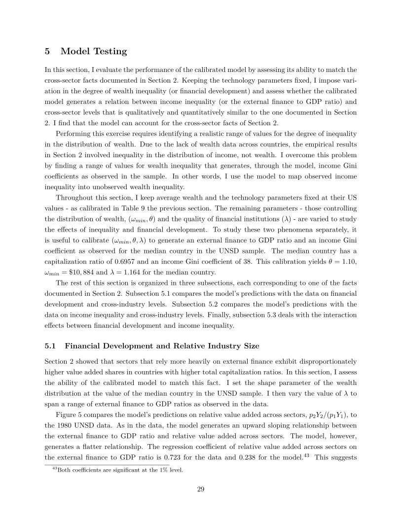
5 Model Testing

In this section, I evaluate the performance of the calibrated model by assessing its ability to match thecross-sector facts documented in Section 2. Keeping the technology parameters fixed, I impose vari-ation in the degree of wealth inequality (or financial development) and assess whether the calibratedmodel generates a relation between income inequality (or the external finance to GDP ratio) andcross-sector levels that is qualitatively and quantitatively similar to the one documented in Section2. I find that the model can account for the cross-sector facts of Section 2.

Performing this exercise requires identifying a realistic range of values for the degree of inequalityin the distribution of wealth. Due to the lack of wealth data across countries, the empirical resultsin Section 2 involved inequality in the distribution of income, not wealth. I overcome this problemby finding a range of values for wealth inequality that generates, through the model, income Ginicoefficients as observed in the sample. In other words, I use the model to map observed incomeinequality into unobserved wealth inequality.

Throughout this section, I keep average wealth and the technology parameters fixed at their USvalues - as calibrated in Table 9 the previous section. The remaining parameters - those controllingthe distribution of wealth, (ωmin, θ) and the quality of financial institutions (λ) - are varied to studythe effects of inequality and financial development. To study these two phenomena separately, itis useful to calibrate (ωmin, θ, λ) to generate an external finance to GDP ratio and an income Ginicoefficient as observed for the median country in the UNSD sample. The median country has acapitalization ratio of 0.6957 and an income Gini coefficient of 38. This calibration yields θ = 1.10,ωmin = $10, 884 and λ = 1.164 for the median country.

The rest of this section is organized in three subsections, each corresponding to one of the factsdocumented in Section 2. Subsection 5.1 compares the model’s predictions with the data on financialdevelopment and cross-industry levels. Subsection 5.2 compares the model’s predictions with thedata on income inequality and cross-industry levels. Finally, subsection 5.3 deals with the interactioneffects between financial development and income inequality.

5.1 Financial Development and Relative Industry Size

Section 2 showed that sectors that rely more heavily on external finance exhibit disproportionatelyhigher value added shares in countries with higher total capitalization ratios. In this section, I assessthe ability of the calibrated model to match this fact. I set the shape parameter of the wealthdistribution at the value of the median country in the UNSD sample. I then vary the value of λ tospan a range of external finance to GDP ratios as observed in the data.

Figure 5 compares the model’s predictions on relative value added across sectors, p2Y2/(p1Y1), tothe 1980 UNSD data. As in the data, the model generates an upward sloping relationship betweenthe external finance to GDP ratio and relative value added across sectors. The model, however,generates a flatter relationship. The regression coefficient of relative value added across sectors onthe external finance to GDP ratio is 0.723 for the data and 0.238 for the model.43 This suggests

43Both coefficients are significant at the 1% level.

29

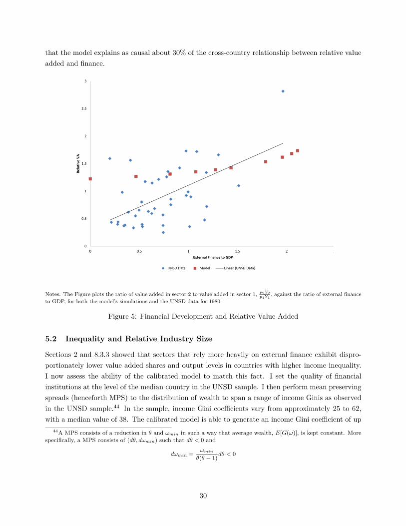
that the model explains as causal about 30% of the cross-country relationship between relative valueadded and finance.

1

1.5

2

2.5

3R

ela

tiv

e V

A

0

0.5

1

0 0.5 1 1.5 2 2.5

External Finance to GDP

UNSD Data Model Linear (UNSD Data)

Notes: The Figure plots the ratio of value added in sector 2 to value added in sector 1, p2Y2p1Y1

, against the ratio of external financeto GDP, for both the model’s simulations and the UNSD data for 1980.

Figure 5: Financial Development and Relative Value Added

5.2 Inequality and Relative Industry Size

Sections 2 and 8.3.3 showed that sectors that rely more heavily on external finance exhibit dispro-portionately lower value added shares and output levels in countries with higher income inequality.I now assess the ability of the calibrated model to match this fact. I set the quality of financialinstitutions at the level of the median country in the UNSD sample. I then perform mean preservingspreads (henceforth MPS) to the distribution of wealth to span a range of income Ginis as observedin the UNSD sample.44 In the sample, income Gini coefficients vary from approximately 25 to 62,with a median value of 38. The calibrated model is able to generate an income Gini coefficient of up

44A MPS consists of a reduction in θ and ωmin in such a way that average wealth, E[G(ω)], is kept constant. Morespecifically, a MPS consists of (dθ, dωmin) such that dθ < 0 and

dωmin = ωminθ(θ − 1)dθ < 0

30

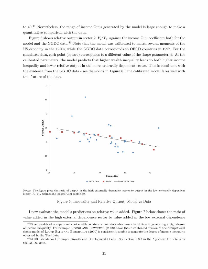
to 40.45 Nevertheless, the range of income Ginis generated by the model is large enough to make aquantitative comparison with the data.

Figure 6 shows relative output in sector 2, Y2/Y1, against the income Gini coefficient both for themodel and the GGDC data.46 Note that the model was calibrated to match several moments of theUS economy in the 1980s, while the GGDC data corresponds to OECD countries in 1997. For thesimulated data, each point (square) corresponds to a different value of the shape parameter, θ. At thecalibrated parameters, the model predicts that higher wealth inequality leads to both higher incomeinequality and lower relative output in the more externally dependent sector. This is consistent withthe evidence from the GGDC data - see diamonds in Figure 6. The calibrated model fares well withthis feature of the data.

1

1.5

2

2.5

3

Re

lati

ve

Ou

tpu

t

0

0.5

1

20 25 30 35 40 45

Income Gini

GGDC Data Model Linear (GGDC Data)

Notes: The figure plots the ratio of output in the high externally dependent sector to output in the low externally dependentsector, Y2/Y1, against the income Gini coefficient.

Figure 6: Inequality and Relative Output: Model vs Data

I now evaluate the model’s predictions on relative value added. Figure 7 below shows the ratio ofvalue added in the high external dependence sector to value added in the low external dependence

45Other models of occupational choice with collateral constraints also have a hard time in generating a high degreeof income inequality. For example, Jeong and Townsend (2008) show that a calibrated version of the occupationalchoice model of Lloyd-Ellis and Bernhardt (2000) is consistently unable to generate the degree of income inequalityobserved in the Thai data.

46GGDC stands for Groningen Growth and Development Centre. See Section 8.3.3 in the Appendix for details onthe GGDC data.

31

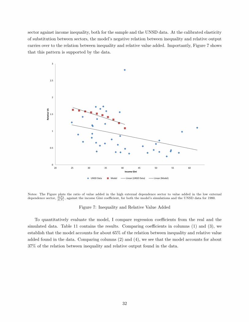
sector against income inequality, both for the sample and the UNSD data. At the calibrated elasticityof substitution between sectors, the model’s negative relation between inequality and relative outputcarries over to the relation between inequality and relative value added. Importantly, Figure 7 showsthat this pattern is supported by the data.

1

1.5

2

2.5

3

Re

lativ

e V

A

0

0.5

1

20 25 30 35 40 45 50 55 60 65

Income Gini

UNSD Data Model Linear (UNSD Data) Linear (Model)

Notes: The Figure plots the ratio of value added in the high external dependence sector to value added in the low externaldependence sector, p2Y2

p1Y1, against the income Gini coefficient, for both the model’s simulations and the UNSD data for 1980.

Figure 7: Inequality and Relative Value Added

To quantitatively evaluate the model, I compare regression coefficients from the real and thesimulated data. Table 11 contains the results. Comparing coefficients in columns (1) and (3), weestablish that the model accounts for about 65% of the relation between inequality and relative valueadded found in the data. Comparing columns (2) and (4), we see that the model accounts for about37% of the relation between inequality and relative output found in the data.

32

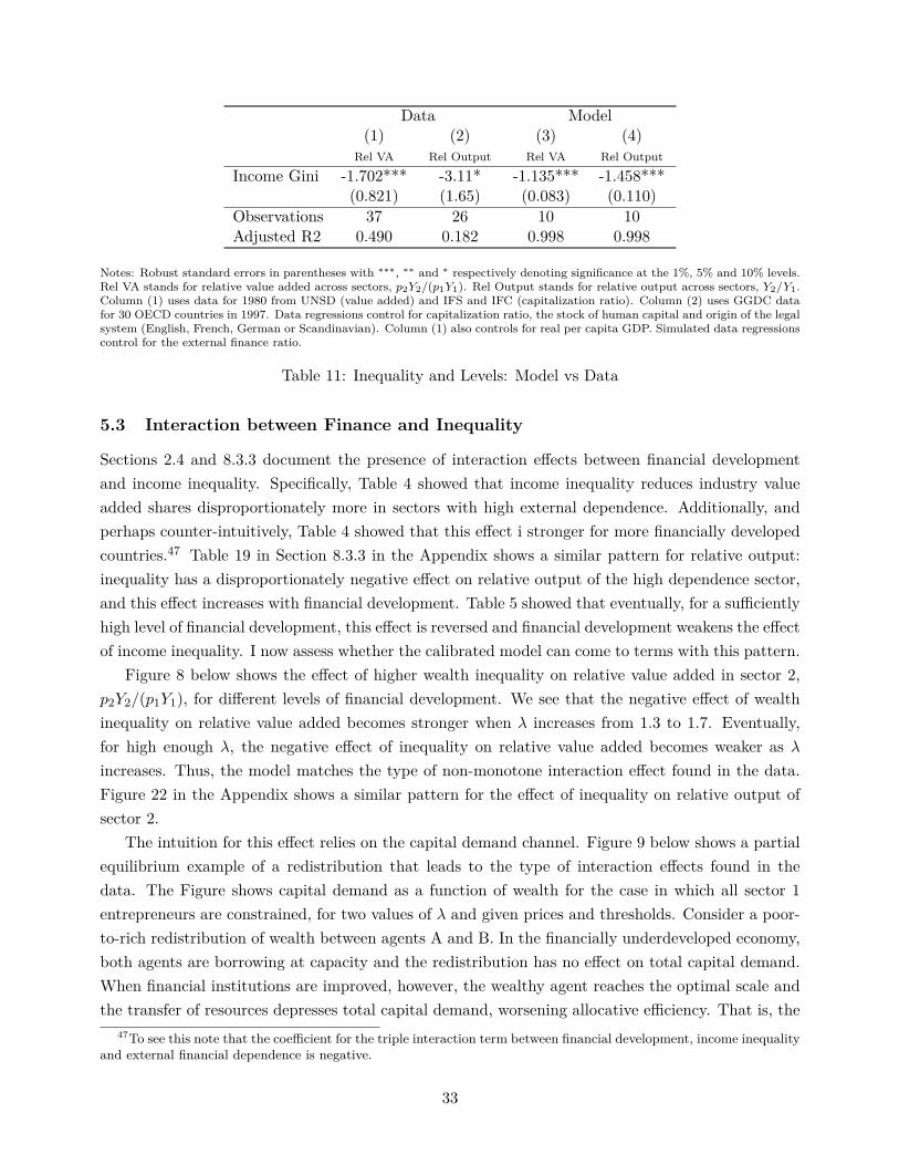
Data Model(1) (2) (3) (4)

Rel VA Rel Output Rel VA Rel Output

Income Gini -1.702*** -3.11* -1.135*** -1.458***(0.821) (1.65) (0.083) (0.110)

Observations 37 26 10 10Adjusted R2 0.490 0.182 0.998 0.998

Notes: Robust standard errors in parentheses with ∗∗∗, ∗∗ and ∗ respectively denoting significance at the 1%, 5% and 10% levels.Rel VA stands for relative value added across sectors, p2Y2/(p1Y1). Rel Output stands for relative output across sectors, Y2/Y1.Column (1) uses data for 1980 from UNSD (value added) and IFS and IFC (capitalization ratio). Column (2) uses GGDC datafor 30 OECD countries in 1997. Data regressions control for capitalization ratio, the stock of human capital and origin of the legalsystem (English, French, German or Scandinavian). Column (1) also controls for real per capita GDP. Simulated data regressionscontrol for the external finance ratio.

Table 11: Inequality and Levels: Model vs Data

5.3 Interaction between Finance and Inequality

Sections 2.4 and 8.3.3 document the presence of interaction effects between financial developmentand income inequality. Specifically, Table 4 showed that income inequality reduces industry valueadded shares disproportionately more in sectors with high external dependence. Additionally, andperhaps counter-intuitively, Table 4 showed that this effect i stronger for more financially developedcountries.47 Table 19 in Section 8.3.3 in the Appendix shows a similar pattern for relative output:inequality has a disproportionately negative effect on relative output of the high dependence sector,and this effect increases with financial development. Table 5 showed that eventually, for a sufficientlyhigh level of financial development, this effect is reversed and financial development weakens the effectof income inequality. I now assess whether the calibrated model can come to terms with this pattern.

Figure 8 below shows the effect of higher wealth inequality on relative value added in sector 2,p2Y2/(p1Y1), for different levels of financial development. We see that the negative effect of wealthinequality on relative value added becomes stronger when λ increases from 1.3 to 1.7. Eventually,for high enough λ, the negative effect of inequality on relative value added becomes weaker as λincreases. Thus, the model matches the type of non-monotone interaction effect found in the data.Figure 22 in the Appendix shows a similar pattern for the effect of inequality on relative output ofsector 2.

The intuition for this effect relies on the capital demand channel. Figure 9 below shows a partialequilibrium example of a redistribution that leads to the type of interaction effects found in thedata. The Figure shows capital demand as a function of wealth for the case in which all sector 1entrepreneurs are constrained, for two values of λ and given prices and thresholds. Consider a poor-to-rich redistribution of wealth between agents A and B. In the financially underdeveloped economy,both agents are borrowing at capacity and the redistribution has no effect on total capital demand.When financial institutions are improved, however, the wealthy agent reaches the optimal scale andthe transfer of resources depresses total capital demand, worsening allocative efficiency. That is, the

47To see this note that the coefficient for the triple interaction term between financial development, income inequalityand external financial dependence is negative.

33

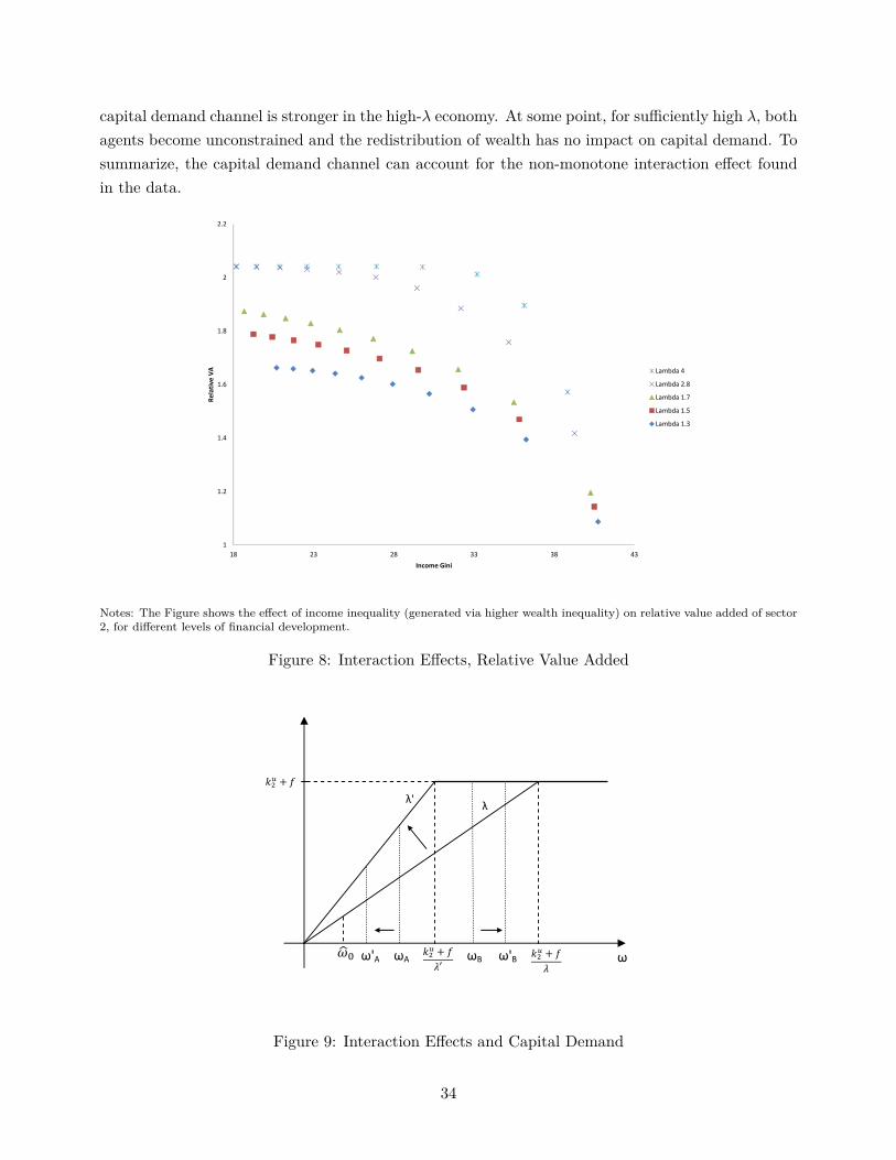
capital demand channel is stronger in the high-λ economy. At some point, for sufficiently high λ, bothagents become unconstrained and the redistribution of wealth has no impact on capital demand. Tosummarize, the capital demand channel can account for the non-monotone interaction effect foundin the data.

1.6

1.8

2

2.2

Re

lativ

e V

A Lambda 4

Lambda 2.8

Lambda 1.7

Lambda 1.5

Lambda 1.3

1

1.2

1.4

18 23 28 33 38 43

Income Gini

Lambda 1.3

Notes: The Figure shows the effect of income inequality (generated via higher wealth inequality) on relative value added of sector2, for different levels of financial development.

Figure 8: Interaction Effects, Relative Value Added

��� + �

�

λ λ'

ω'B ��� + �

�′

��� + �

ωA ω'A � ωB ω

Figure 9: Interaction Effects and Capital Demand

34

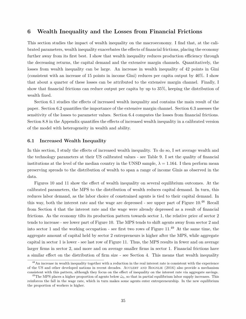
6 Wealth Inequality and the Losses from Financial Frictions

This section studies the impact of wealth inequality on the macroeconomy. I find that, at the cali-brated parameters, wealth inequality exacerbates the effects of financial frictions, placing the economyfurther away from its first best. I show that wealth inequality reduces production efficiency throughthe decreasing returns, the capital demand and the extensive margin channels. Quantitatively, thelosses from wealth inequality can be large. An increase in wealth inequality of 42 points in Gini(consistent with an increase of 15 points in income Gini) reduces per capita output by 46%. I showthat about a quarter of these losses can be attributed to the extensive margin channel. Finally, Ishow that financial frictions can reduce output per capita by up to 35%, keeping the distribution ofwealth fixed.

Section 6.1 studies the effects of increased wealth inequality and contains the main result of thepaper. Section 6.2 quantifies the importance of the extensive margin channel. Section 6.3 assesses thesensitivity of the losses to parameter values. Section 6.4 computes the losses from financial frictions.Section 8.8 in the Appendix quantifies the effects of increased wealth inequality in a calibrated versionof the model with heterogeneity in wealth and ability.

6.1 Increased Wealth Inequality

In this section, I study the effects of increased wealth inequality. To do so, I set average wealth andthe technology parameters at their US calibrated values - see Table 9. I set the quality of financialinstitutions at the level of the median country in the UNSD sample, λ = 1.164. I then perform meanpreserving spreads to the distribution of wealth to span a range of income Ginis as observed in thedata.

Figures 10 and 11 show the effect of wealth inequality on several equilibrium outcomes. At thecalibrated parameters, the MPS to the distribution of wealth reduces capital demand. In turn, thisreduces labor demand, as the labor choice of constrained agents is tied to their capital demand. Inthis way, both the interest rate and the wage are depressed - see upper part of Figure 10.48 Recallfrom Section 4 that the interest rate and the wage were already depressed as a result of financialfrictions. As the economy tilts its production pattern towards sector 1, the relative price of sector 2tends to increase - see lower part of Figure 10. The MPS tends to shift agents away from sector 2 andinto sector 1 and the working occupation - see first two rows of Figure 11.49 At the same time, theaggregate amount of capital held by sector 2 entrepreneurs is higher after the MPS, while aggregatecapital in sector 1 is lower - see last row of Figure 11. Thus, the MPS results in fewer and on averagelarger firms in sector 2, and more and on average smaller firms in sector 1. Financial frictions havea similar effect on the distribution of firm size - see Section 4. This means that wealth inequality

48An increase in wealth inequality together with a reduction in the real interest rate is consistent with the experienceof the US and other developed nations in recent decades. Auclert and Rognlie (2016) also provide a mechanismconsistent with this pattern, although they focus on the effect of inequality on the interest rate via aggregate savings.

49The MPS places a higher proportion of agents below ω0, so that in partial equilibrium labor supply increases. Thisreinforces the fall in the wage rate, which in turn makes some agents enter entrepreneurship. In the new equilibriumthe proportion of workers is higher.

35

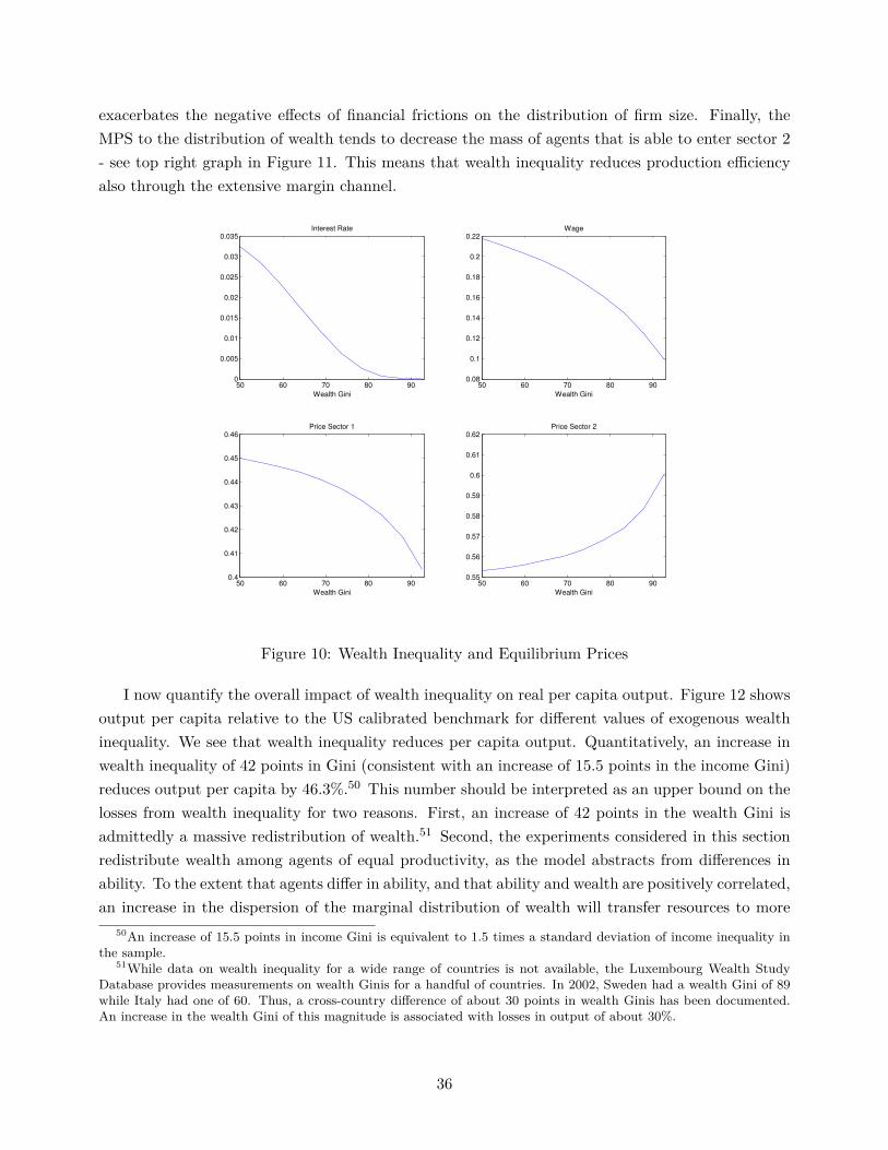
exacerbates the negative effects of financial frictions on the distribution of firm size. Finally, theMPS to the distribution of wealth tends to decrease the mass of agents that is able to enter sector 2- see top right graph in Figure 11. This means that wealth inequality reduces production efficiencyalso through the extensive margin channel.

50 60 70 80 900

0.005

0.01

0.015

0.02

0.025

0.03

0.035

Wealth Gini

Interest Rate

50 60 70 80 900.08

0.1

0.12

0.14

0.16

0.18

0.2

0.22

Wealth Gini

Wage

50 60 70 80 900.4

0.41

0.42

0.43

0.44

0.45

0.46

Wealth Gini

Price Sector 1

50 60 70 80 900.55

0.56

0.57

0.58

0.59

0.6

0.61

0.62

Wealth Gini

Price Sector 2

Figure 10: Wealth Inequality and Equilibrium Prices

I now quantify the overall impact of wealth inequality on real per capita output. Figure 12 showsoutput per capita relative to the US calibrated benchmark for different values of exogenous wealthinequality. We see that wealth inequality reduces per capita output. Quantitatively, an increase inwealth inequality of 42 points in Gini (consistent with an increase of 15.5 points in the income Gini)reduces output per capita by 46.3%.50 This number should be interpreted as an upper bound on thelosses from wealth inequality for two reasons. First, an increase of 42 points in the wealth Gini isadmittedly a massive redistribution of wealth.51 Second, the experiments considered in this sectionredistribute wealth among agents of equal productivity, as the model abstracts from differences inability. To the extent that agents differ in ability, and that ability and wealth are positively correlated,an increase in the dispersion of the marginal distribution of wealth will transfer resources to more

50An increase of 15.5 points in income Gini is equivalent to 1.5 times a standard deviation of income inequality inthe sample.

51While data on wealth inequality for a wide range of countries is not available, the Luxembourg Wealth StudyDatabase provides measurements on wealth Ginis for a handful of countries. In 2002, Sweden had a wealth Gini of 89while Italy had one of 60. Thus, a cross-country difference of about 30 points in wealth Ginis has been documented.An increase in the wealth Gini of this magnitude is associated with losses in output of about 30%.

36

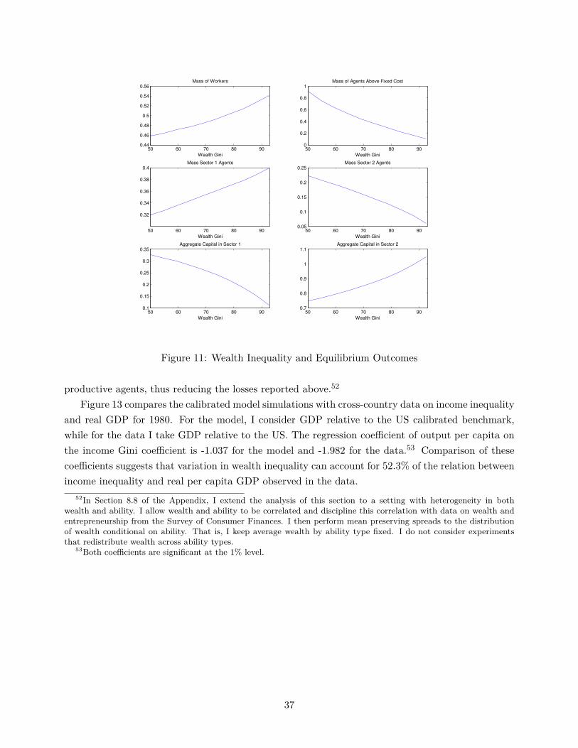
50 60 70 80 900.44

0.46

0.48

0.5

0.52

0.54

0.56

Wealth Gini

Mass of Workers

50 60 70 80 900

0.2

0.4

0.6

0.8

1

Wealth Gini

Mass of Agents Above Fixed Cost

50 60 70 80 90

0.32

0.34

0.36

0.38

0.4

Wealth Gini

Mass Sector 1 Agents

50 60 70 80 900.05

0.1

0.15

0.2

0.25

Wealth Gini

Mass Sector 2 Agents

50 60 70 80 900.1

0.15

0.2

0.25

0.3

0.35

Wealth Gini

Aggregate Capital in Sector 1

50 60 70 80 900.7

0.8

0.9

1

1.1

Wealth Gini

Aggregate Capital in Sector 2

Figure 11: Wealth Inequality and Equilibrium Outcomes

productive agents, thus reducing the losses reported above.52

Figure 13 compares the calibrated model simulations with cross-country data on income inequalityand real GDP for 1980. For the model, I consider GDP relative to the US calibrated benchmark,while for the data I take GDP relative to the US. The regression coefficient of output per capita onthe income Gini coefficient is -1.037 for the model and -1.982 for the data.53 Comparison of thesecoefficients suggests that variation in wealth inequality can account for 52.3% of the relation betweenincome inequality and real per capita GDP observed in the data.

52In Section 8.8 of the Appendix, I extend the analysis of this section to a setting with heterogeneity in bothwealth and ability. I allow wealth and ability to be correlated and discipline this correlation with data on wealth andentrepreneurship from the Survey of Consumer Finances. I then perform mean preserving spreads to the distributionof wealth conditional on ability. That is, I keep average wealth by ability type fixed. I do not consider experimentsthat redistribute wealth across ability types.

53Both coefficients are significant at the 1% level.

37

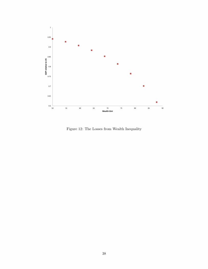
0.75

0.8

0.85

0.9

0.95

1

GD

P r

ela

tiv

e t

o U

S

0.6

0.65

0.7

0.75

50 55 60 65 70 75 80 85 90

Wealth Gini

Figure 12: The Losses from Wealth Inequality

38

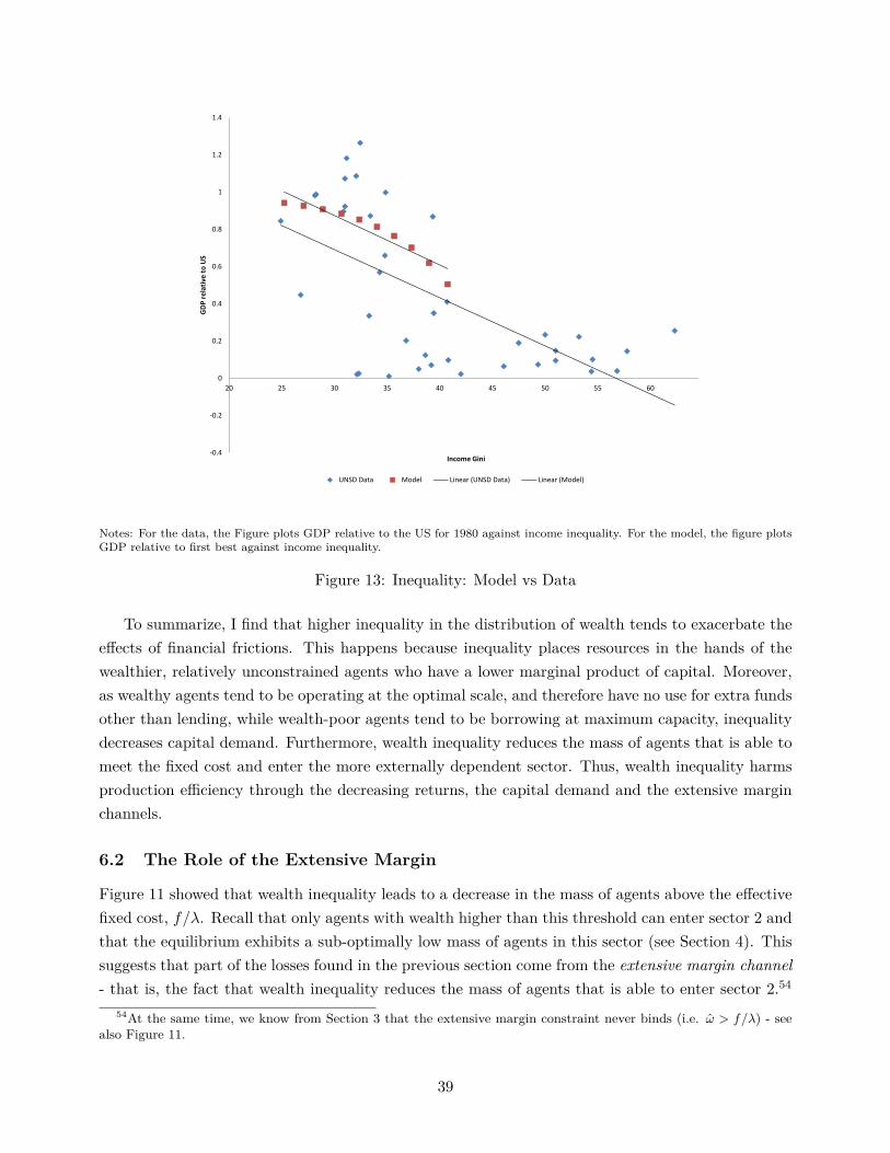
0.4

0.6

0.8

1

1.2

1.4

GD

P r

ela

tiv

e t

o U

S

-0.4

-0.2

0

0.2

20 25 30 35 40 45 50 55 60 65

Income Gini

UNSD Data Model Linear (UNSD Data) Linear (Model)

Notes: For the data, the Figure plots GDP relative to the US for 1980 against income inequality. For the model, the figure plotsGDP relative to first best against income inequality.

Figure 13: Inequality: Model vs Data

To summarize, I find that higher inequality in the distribution of wealth tends to exacerbate theeffects of financial frictions. This happens because inequality places resources in the hands of thewealthier, relatively unconstrained agents who have a lower marginal product of capital. Moreover,as wealthy agents tend to be operating at the optimal scale, and therefore have no use for extra fundsother than lending, while wealth-poor agents tend to be borrowing at maximum capacity, inequalitydecreases capital demand. Furthermore, wealth inequality reduces the mass of agents that is able tomeet the fixed cost and enter the more externally dependent sector. Thus, wealth inequality harmsproduction efficiency through the decreasing returns, the capital demand and the extensive marginchannels.

6.2 The Role of the Extensive Margin

Figure 11 showed that wealth inequality leads to a decrease in the mass of agents above the effectivefixed cost, f/λ. Recall that only agents with wealth higher than this threshold can enter sector 2 andthat the equilibrium exhibits a sub-optimally low mass of agents in this sector (see Section 4). Thissuggests that part of the losses found in the previous section come from the extensive margin channel- that is, the fact that wealth inequality reduces the mass of agents that is able to enter sector 2.54

54At the same time, we know from Section 3 that the extensive margin constraint never binds (i.e. ω > f/λ) - seealso Figure 11.

39

To quantify the importance of this channel, I perform the following exercise. I consider the problemof a planner that can freely assign capital and labor to agents, and agents to sectors, subject to anexogenous constraint on the mass of agents that can be assigned to sector 2. Specifically, letting µ0

and µ denote the mass of workers and sector 1 entrepreneurs respectively, the planner’s problem isgiven by:

maxk1,k2,l1,l2,µ,µ0

A[γ(µkαν1 l

(1−α)ν1 )

ε−1ε + (1− γ) ((1− µ− µ0) kαν2 l

(1−α)ν2 )

ε−1ε

] εε−1 + (1− δ)E [ω]

subject toµk1 + (1− µ− µ0) (k2 + f) = E [ω]

µl1 + (1− µ− µ0) l2 = µ0

1− µ− µ0 ≤ c

I keep the technology parameters and average wealth at their calibrated values. I study the lossesin output per capita arising from variation in the maximum amount of agents that can be assignedto sector 2 (i.e. c). In particular, I decrease c from about 22% to 6%, which is the range for themass of agents allocated to sector 2 that results from variation in wealth inequality, as obtained inthe previous section - see Figure 11. Figure 14 contains the results. We see that a decrease in themaximum amount of agents that can be assigned to sector 2 from 22% to 6% leads to a reductionin output per capita of about 10%. This amounts to a quarter of the losses from wealth inequalityfound in the previous section.

40

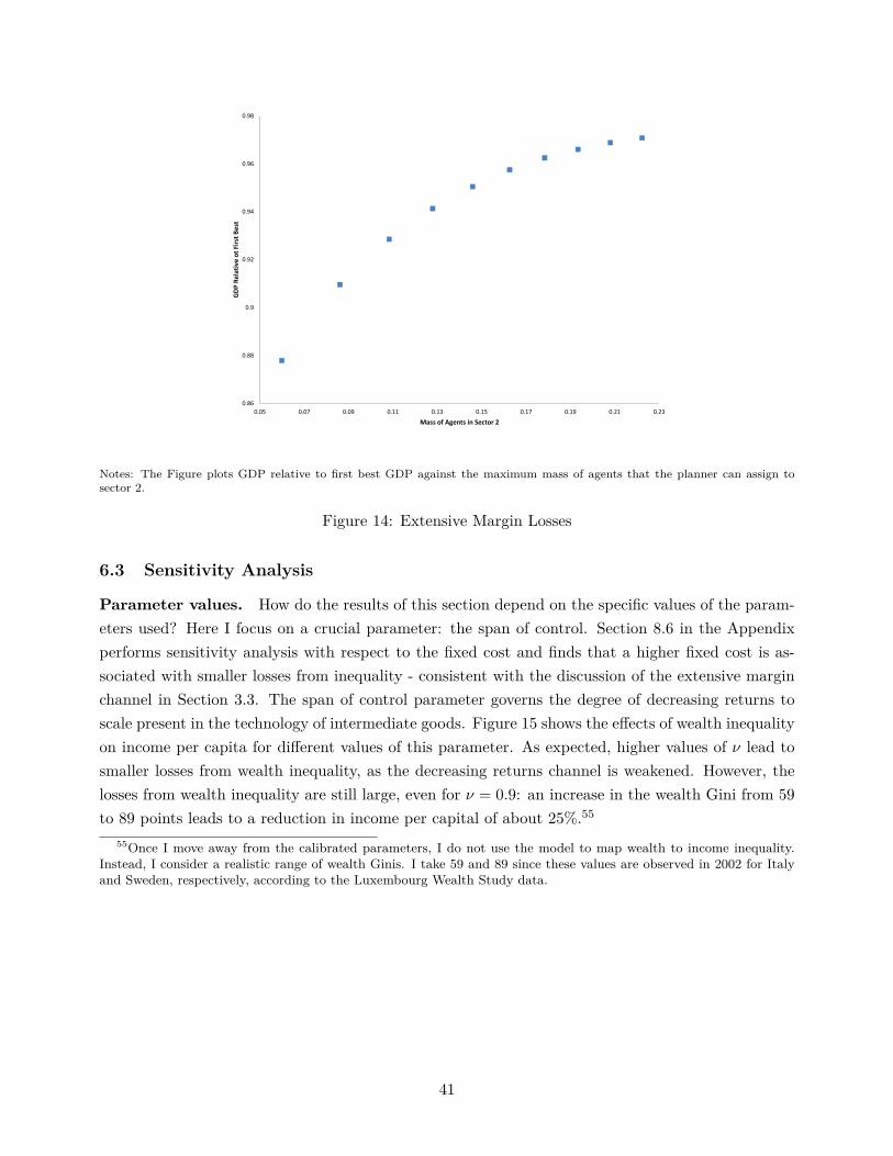
0.92

0.94

0.96

0.98

GD

P R

ela

tiv

e o

t F

irst

Be

st

0.86

0.88

0.9

0.05 0.07 0.09 0.11 0.13 0.15 0.17 0.19 0.21 0.23

GD

P R

ela

tiv

e o

t F

irst

Be

st

Mass of Agents in Sector 2

Notes: The Figure plots GDP relative to first best GDP against the maximum mass of agents that the planner can assign tosector 2.

Figure 14: Extensive Margin Losses

6.3 Sensitivity Analysis

Parameter values. How do the results of this section depend on the specific values of the param-eters used? Here I focus on a crucial parameter: the span of control. Section 8.6 in the Appendixperforms sensitivity analysis with respect to the fixed cost and finds that a higher fixed cost is as-sociated with smaller losses from inequality - consistent with the discussion of the extensive marginchannel in Section 3.3. The span of control parameter governs the degree of decreasing returns toscale present in the technology of intermediate goods. Figure 15 shows the effects of wealth inequalityon income per capita for different values of this parameter. As expected, higher values of ν lead tosmaller losses from wealth inequality, as the decreasing returns channel is weakened. However, thelosses from wealth inequality are still large, even for ν = 0.9: an increase in the wealth Gini from 59to 89 points leads to a reduction in income per capital of about 25%.55

55Once I move away from the calibrated parameters, I do not use the model to map wealth to income inequality.Instead, I consider a realistic range of wealth Ginis. I take 59 and 89 since these values are observed in 2002 for Italyand Sweden, respectively, according to the Luxembourg Wealth Study data.

41

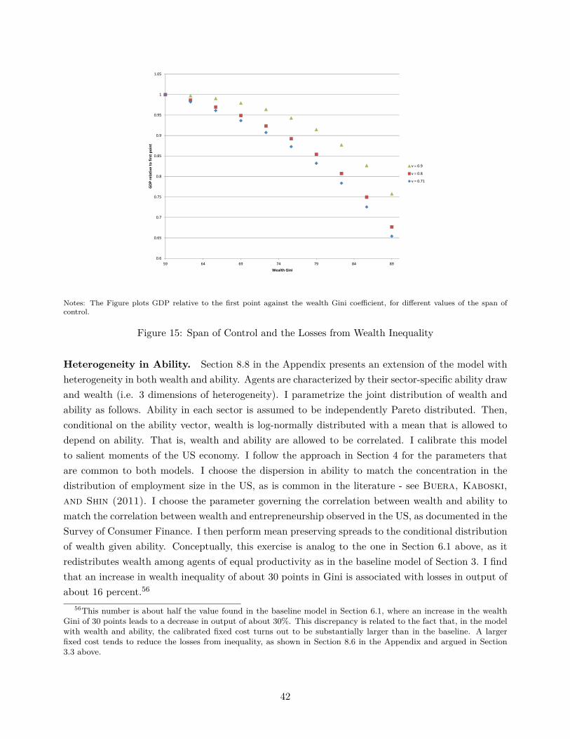
0.8

0.85

0.9

0.95

1

1.05

GD

P r

ela

tiv

e t

o f

irst

po

int

v = 0.9

v = 0.8

v = 0.71

0.6

0.65

0.7

0.75

59 64 69 74 79 84 89

GD

P r

ela

tiv

e t

o f

irst

po

int

Wealth Gini

Notes: The Figure plots GDP relative to the first point against the wealth Gini coefficient, for different values of the span ofcontrol.

Figure 15: Span of Control and the Losses from Wealth Inequality

Heterogeneity in Ability. Section 8.8 in the Appendix presents an extension of the model withheterogeneity in both wealth and ability. Agents are characterized by their sector-specific ability drawand wealth (i.e. 3 dimensions of heterogeneity). I parametrize the joint distribution of wealth andability as follows. Ability in each sector is assumed to be independently Pareto distributed. Then,conditional on the ability vector, wealth is log-normally distributed with a mean that is allowed todepend on ability. That is, wealth and ability are allowed to be correlated. I calibrate this modelto salient moments of the US economy. I follow the approach in Section 4 for the parameters thatare common to both models. I choose the dispersion in ability to match the concentration in thedistribution of employment size in the US, as is common in the literature - see Buera, Kaboski,and Shin (2011). I choose the parameter governing the correlation between wealth and ability tomatch the correlation between wealth and entrepreneurship observed in the US, as documented in theSurvey of Consumer Finance. I then perform mean preserving spreads to the conditional distributionof wealth given ability. Conceptually, this exercise is analog to the one in Section 6.1 above, as itredistributes wealth among agents of equal productivity as in the baseline model of Section 3. I findthat an increase in wealth inequality of about 30 points in Gini is associated with losses in output ofabout 16 percent.56

56This number is about half the value found in the baseline model in Section 6.1, where an increase in the wealthGini of 30 points leads to a decrease in output of about 30%. This discrepancy is related to the fact that, in the modelwith wealth and ability, the calibrated fixed cost turns out to be substantially larger than in the baseline. A largerfixed cost tends to reduce the losses from inequality, as shown in Section 8.6 in the Appendix and argued in Section3.3 above.

42

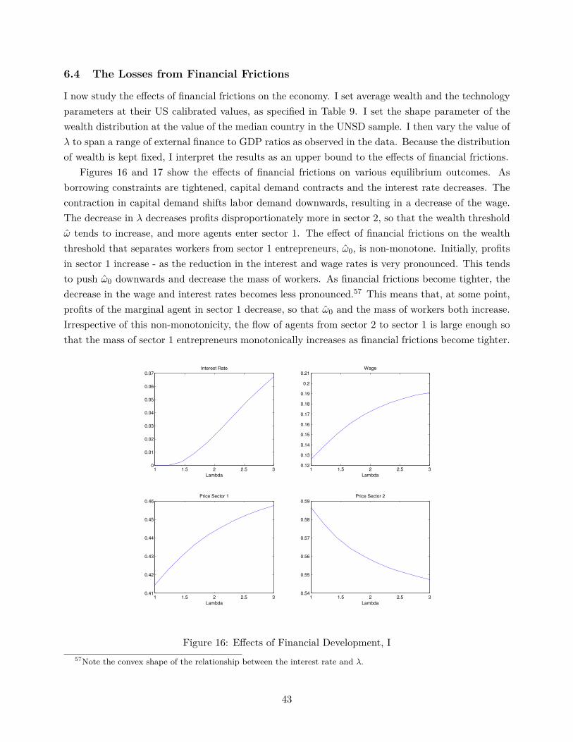
6.4 The Losses from Financial Frictions

I now study the effects of financial frictions on the economy. I set average wealth and the technologyparameters at their US calibrated values, as specified in Table 9. I set the shape parameter of thewealth distribution at the value of the median country in the UNSD sample. I then vary the value ofλ to span a range of external finance to GDP ratios as observed in the data. Because the distributionof wealth is kept fixed, I interpret the results as an upper bound to the effects of financial frictions.

Figures 16 and 17 show the effects of financial frictions on various equilibrium outcomes. Asborrowing constraints are tightened, capital demand contracts and the interest rate decreases. Thecontraction in capital demand shifts labor demand downwards, resulting in a decrease of the wage.The decrease in λ decreases profits disproportionately more in sector 2, so that the wealth thresholdω tends to increase, and more agents enter sector 1. The effect of financial frictions on the wealththreshold that separates workers from sector 1 entrepreneurs, ω0, is non-monotone. Initially, profitsin sector 1 increase - as the reduction in the interest and wage rates is very pronounced. This tendsto push ω0 downwards and decrease the mass of workers. As financial frictions become tighter, thedecrease in the wage and interest rates becomes less pronounced.57 This means that, at some point,profits of the marginal agent in sector 1 decrease, so that ω0 and the mass of workers both increase.Irrespective of this non-monotonicity, the flow of agents from sector 2 to sector 1 is large enough sothat the mass of sector 1 entrepreneurs monotonically increases as financial frictions become tighter.

1 1.5 2 2.5 30

0.01

0.02

0.03

0.04

0.05

0.06

0.07

Lambda

Interest Rate

1 1.5 2 2.5 30.12

0.13

0.14

0.15

0.16

0.17

0.18

0.19

0.2

0.21

Lambda

Wage

1 1.5 2 2.5 30.41

0.42

0.43

0.44

0.45

0.46

Lambda

Price Sector 1

1 1.5 2 2.5 30.54

0.55

0.56

0.57

0.58

0.59

Lambda

Price Sector 2

Figure 16: Effects of Financial Development, I57Note the convex shape of the relationship between the interest rate and λ.

43

1 1.5 2 2.5 30.512

0.514

0.516

0.518

0.52

0.522

0.524

0.526

0.528

Lambda

Mass of Workers

1 1.5 2 2.5 30.1

0.2

0.3

0.4

0.5

0.6

Lambda

Mass of Agents Above Fixed Cost

1 1.5 2 2.5 3

0.3

0.32

0.34

0.36

0.38

0.4

Lambda

Mass Sector 1 Agents

1 1.5 2 2.5 30.08

0.1

0.12

0.14

0.16

0.18

Lambda

Mass Sector 2 Agents

Figure 17: Effects of Financial Development, II

Figure 18 quantifies the overall impact of financial frictions on output per worker. It depictsoutput per capita relative to the US calibrated benchmark for different values of λ. We see that, inthe calibrated model, financial frictions can reduce output to about 65% of the US level. In termsof observables, Figure 19 shows the cross-country relation between the ratio of external finance toGDP and output per capita relative to the US, both for the data and the model simulations, aftercontrolling for income inequality. That is, for the data, I remove the variation stemming from incomeinequality.58 The regression coefficient of output per capita on the ratio of external finance to GDPis 0.163 for the model and 0.23 for the data (controlling for the income Gini).59 Comparison of thesecoefficients suggests that variation in the quality of financial institutions can account for about 70%of the cross country relation between finance and GDP observed in the data.

58That is, I plot the residuals of a regression of output per capita relative to the US on the income Gini. For themodel, I report output relative to the first best, demeaned.

59Both coefficients are significant at the 10% level.

44

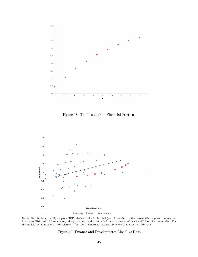
0.8

0.85

0.9

0.95

1

1.05

GD

P r

ela

tiv

e t

o U

S

0.6

0.65

0.7

0.75

1 1.2 1.4 1.6 1.8 2 2.2 2.4 2.6 2.8 3

λ

Figure 18: The Losses from Financial Frictions

-0.8

-0.6

-0.4

-0.2

0

0.2

0.4

0.6

0.8

0 0.5 1 1.5 2 2.5

GDPrelativ

etoUS

ExternalFinancetoGDP

UNSDData Model Linear(UNSDData)

Notes: For the data, the Figure plots GDP relative to the US in 1980 (net of the effect of the income Gini) against the externalfinance to GDP ratio. More precisely, the y-axis depicts the residuals from a regression of relative GDP on the income Gini. Forthe model, the figure plots GDP relative to first best (demeaned) against the external finance to GDP ratio.

Figure 19: Finance and Development: Model vs Data

45

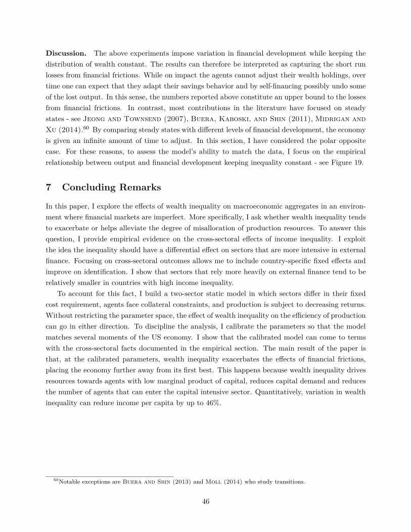
Discussion. The above experiments impose variation in financial development while keeping thedistribution of wealth constant. The results can therefore be interpreted as capturing the short runlosses from financial frictions. While on impact the agents cannot adjust their wealth holdings, overtime one can expect that they adapt their savings behavior and by self-financing possibly undo someof the lost output. In this sense, the numbers reported above constitute an upper bound to the lossesfrom financial frictions. In contrast, most contributions in the literature have focused on steadystates - see Jeong and Townsend (2007), Buera, Kaboski, and Shin (2011), Midrigan andXu (2014).60 By comparing steady states with different levels of financial development, the economyis given an infinite amount of time to adjust. In this section, I have considered the polar oppositecase. For these reasons, to assess the model’s ability to match the data, I focus on the empiricalrelationship between output and financial development keeping inequality constant - see Figure 19.

7 Concluding Remarks

In this paper, I explore the effects of wealth inequality on macroeconomic aggregates in an environ-ment where financial markets are imperfect. More specifically, I ask whether wealth inequality tendsto exacerbate or helps alleviate the degree of misallocation of production resources. To answer thisquestion, I provide empirical evidence on the cross-sectoral effects of income inequality. I exploitthe idea the inequality should have a differential effect on sectors that are more intensive in externalfinance. Focusing on cross-sectoral outcomes allows me to include country-specific fixed effects andimprove on identification. I show that sectors that rely more heavily on external finance tend to berelatively smaller in countries with high income inequality.

To account for this fact, I build a two-sector static model in which sectors differ in their fixedcost requirement, agents face collateral constraints, and production is subject to decreasing returns.Without restricting the parameter space, the effect of wealth inequality on the efficiency of productioncan go in either direction. To discipline the analysis, I calibrate the parameters so that the modelmatches several moments of the US economy. I show that the calibrated model can come to termswith the cross-sectoral facts documented in the empirical section. The main result of the paper isthat, at the calibrated parameters, wealth inequality exacerbates the effects of financial frictions,placing the economy further away from its first best. This happens because wealth inequality drivesresources towards agents with low marginal product of capital, reduces capital demand and reducesthe number of agents that can enter the capital intensive sector. Quantitatively, variation in wealthinequality can reduce income per capita by up to 46%.

60Notable exceptions are Buera and Shin (2013) and Moll (2014) who study transitions.

46

References

Acemoglu, D., and V. Guerrieri (2008): “Capital Deepening and Nonbalanced EconomicGrowth,” Journal of Political Economy, 116(3), 467–498.

Acemoglu, D., and J. A. Robinson (2000): “Why did the West extend the franchise? Democracy,inequality, and growth in historical perspective,” The Quarterly Journal of Economics, 115(4),1167–1199.

Alesina, A., G. Cozzi, and N. Mantovan (2012): “The evolution of ideology, fairness andredistribution,” The Economic Journal, 122(565), 1244–1261.

Alesina, A., and R. Perotti (1996): “Income Distribution, Political Instability and Investment,”European Economic Review, 81(5), 1170–1189.

Alesina, A., and D. Rodrik (1994): “Distributive Politics and Economic Growth,” QuarterlyJournal of Economics, 109(2), 465–490.

Alesina, A. F., and P. Giuliano (2009): “Preferences for redistribution,” Discussion paper,National Bureau of Economic Research.

Auclert, A., and M. Rognlie (2016): “Inequality and aggregate demand,” Unpublished Paper.

Banerjee, A., and E. Duflo (2005): “Growth Theory through the Lens of Development Eco-nomics,” in Handbook of Economic Growth, ed. by P. Aghion, and S. Durlauf, vol. 1A, chap. 7, pp.473–552. Elsevier B.V.

Banerjee, A., and A. Newman (1993): “Occupational Choice and the Process of Develop,” Jour-nal of Political Economy, 101(2), 274–298.

(2003): “Inequality, Growth, and Trade Policy,” .

Banerjee, A. V., and E. Duflo (2003): “Inequality and Growth: What Can the Data Say?,”Journal of economic growth, 8(3), 267–299.

Beck, T., A. Demirgüç-Kunt, and R. Levine (2000): “A New Database on Financial Develop-ment and Structure,” World Bank Economic Review, 14, 597–605.

Blanchflower, D., and A. Oswald (1998): “What makes a Young Entrepreneur?,” Journal ofLabor Economics, 16, 26–60.

Braun, M. (2003): “Financial Contractibility and Asset Hardness,” UCLA Mimeo.

Buera, F., J. Kaboski, and Y. Shin (2011): “Finance and Development: A Tale of Two Sectors,”American Economc Review, 101(5), 1964–2002.

Buera, F. J., and Y. Shin (2013): “Financial frictions and the persistence of history: A quantitativeexploration,” Journal of Political Economy, 121(2), 221–272.

47

Cagetti, M., M. De Nardi, and others (2006): “Entrepreneurship, Frictions, and Wealth,”Journal of political Economy, 114(5), 835–870.

Caselli, F. (2005): “Accounting for Cross-Country Income Differences,” Handbook of economicgrowth, 1, 679–741.

De Nardi, M. (2015): “Quantitative models of wealth inequality: A survey,” Discussion paper,National Bureau of Economic Research.

Deininger, K., and L. Squire (1996): “A new data set measuring income inequality,” World BankEconomic Review, 10, 565–591.

Easterly, W. (2007): “Inequality does cause underdevelopment: Insights from a new instrument,”Journal of Development Economics, 84(2), 755–776.

Engerman, S. L., and K. L. Sokoloff (2000): “History lessons: Institutions, factors endowments,and paths of development in the new world,” The Journal of Economic Perspectives, 14(3), 217–232.

(2002): “Factor endowments, inequality, and paths of development among new world eco-nomics,” Discussion paper, National Bureau of Economic Research.

Evans, D., and L. Leighton (1989): “Some Empirical Aspects of Entrepreneurship,” AmericanEconomic Review, 79, 519–535.

Evans, D. S., and B. Jovanovic (1989): “An Estimated Model of Entrepreneurial Choice underLiquidity Constraints,” Journal of Political Economy, 97(4).

Forbes, K. (2000): “A reassessment of the relationship between inequality and growth,” AmericanEconomic Review, 90(4), 869–887.

Galor, O., and J. Zeira (1993): “Income Distribution and Macroeconomics,” Review of EconomicStudies, 60(1), 35–52.

Greenwood, J., and B. Jovanovic (1990): “Financial Development, Growth and the Distributionof Income,” Journal of Political Economy, 98(5), 1076–1107.

Guerrieri, V., and G. Lorenzoni (2017): “Credit crises, precautionary savings, and the liquiditytrap,” The Quarterly Journal of Economics, 132(3), 1427–1467.

Holtz-Eakin, D., D. Joulfaian, and H. S. Rosen (1994): “Entrepreneurial Decisions and Liq-uidity Constraints,” Rand Journal of Economics, 25, 334–347.

Hsieh, C.-T., and P. Klenow (2009): “Misallocation and Manufacturing TFP in China and India,”Quarterly Journal of Economics, 124(2), 771–807.

48

Hurst, E., and A. Lusardi (2004): “Liquidity Constraints, Household Wealth and Entrepreneur-ship,” Journal of Political Economy, 112(2), 319–347.

Inklaar, R., and M. Timmer (2008): “GGDC Productivity Level Database: International Com-parisons of Output, Inputs and Productivity at the Industry Level,” Groningen Growth and De-velopment Centre Research Memorandum GD-104.

Jeong, H., and R. Townsend (2007): “Sources of TFP Growth: Occupational Choice and Finan-cial Deepening,” Economic Theory, 32, 179–221.

(2008): “Growth and Inequality: Model Evaluation Based on an Estimation-CalibrationStrategy,” Macroeconomic Dynamics, 12, 231–284.

Klass, O., O. Biham, M. Levy, O. Malcai, and S. Solomon (2006): “The Forbes 400 and thePareto wealth distribution,” Economic Letters, 90(2), 290–295.

Krueger, D., K. Mitman, and F. Perri (2016): “Macroeconomics and Household Heterogeneity,”Handbook of Macroeconomics, 2, 843–921.

Krusell, P., and A. Smith, Jr. (1998): “Income andWealth Heterogeneity in the Macroeconomy,”Journal of Political Economy, 106(5), 867–896.

Li, H., and H. Zou (1998): “Income Inequality is Not Harmful for Growth: Theory and Evidence,”Review of Development Economics, 2(3), 318–334.

Lloyd-Ellis, H., and D. Bernhardt (2000): “Enterprise, Inequality and Economic Develop-ment,” The Review of Economic Studies, 67(1), 147–168.

Lucas, R. E. (1978): “On the Size Distribution of Business Firms,” The Bell Journal of Economics,9(2), 508–523.

Manova, K. (2008): “Credit Constraints, Equity Market Liberalizations and International Trade,”Journal of International Economics, 76, 33–47.

Midrigan, V., and D. Y. Xu (2014): “Finance and misallocation: Evidence from plant-level data,”The American Economic Review, 104(2), 422–458.

Moll, B. (2014): “Productivity losses from financial frictions: can self-financing undo capital mis-allocation?,” The American Economic Review, 104(10), 3186–3221.

Pareto, V. (1897): Cours d’economie politique. Geneve, Droz.

Perotti, R. (1996): “Growth, Income Distribution, and Democracy: What can the data say,”Journal of Economic Growth, 1, 149–187.

Persson, T., and G. Tabellini (1994): “Is Inequality Harmful for Growth?,” American EconomicReview, 84(3), 600–621.

49

Piketty, T. (1997): “The Dynamics of the Wealth Distribution and the Interest Rate with CreditRationing,” Review of Economic Studies, 64, 173–189.

Rajan, R., and L. Zingales (1998): “Financial Dependence and Growth,” The American EconomicReview, 88(3), 559–586.

Restuccia, D., and R. Rogerson (2008): “Policy distortions and aggregate productivity withheterogenous establishments,” Review of Economic Dynamics, 11, 707–720.

United Nations Statistical Division (1993): Industrial Statistics Yearbook, vol. 1. New York:United Nations.

Wolff, E. (1999): The Size Distribution of Wealth in the United States: A Comparison amongRecent Household Surveyschap. I, pp. 209–232.

50

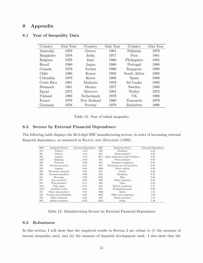
8 Appendix

8.1 Year of Inequality Data

Country Gini Year Country Gini Year Country Gini YearAustralia 1979 Greece 1981 Pakistan 1979Banglades 1978 India 1977 Peru 1981Belgium 1979 Italy 1980 Philippines 1985Brazil 1980 Japan 1980 Portugal 1980Canada 1979 Jordan 1980 Singapore 1980Chile 1980 Kenya 1992 South Africa 1993Colombia 1978 Korea 1980 Spain 1980Costa Rica 1981 Malaysia 1979 Sri Lanka 1980Denmark 1981 Mexico 1977 Sweden 1980Egypt 1975 Morocco 1984 Turkey 1973Finland 1980 Netherlands 1979 UK 1980France 1979 New Zealand 1980 Venezuela 1979Germany 1978 Norway 1979 Zimbabwe 1990

Table 12: Year of initial inequality

8.2 Sectors by External Financial Dependence

The following table displays the 36 3-digit ISIC manufacturing sectors, in order of increasing externalfinancial dependence, as measured in Rajan and Zingales (1998).

ISIC Industrial Sector External Dependence ISIC Industrial Sector External Dependence314 Tobacco -0.45 332 Furniture 0.24361 Pottery -0.15 381 Metal products 0.24323 Leather -0.14 3511 Basic chemicals except fertilizers 0.253211 Spinning -0.09 331 Wood products 0.28324 Footwear -0.08 384 Transport equipment 0.31372 Non-ferrous metal 0.01 354 Petroleum and coal products 0.33322 Apparel 0.03 3843 Motor vehicle 0.39353 Petroleum refineries 0.04 321 Textile 0.40369 Nonmetal products 0.06 382 Machinery 0.45313 Beverages 0.08 3841 Ship 0.46371 Iron and Steel 0.09 390 Other industries 0.47311 Food products 0.14 362 Glass 0.533411 Pulp, paper 0.15 383 Electric machinery 0.773513 Synthetic resins 0.16 385 Professional goods 0.96341 Paper and products 0.18 3832 Radio 1.04342 Printing and publishing 0.20 3825 Office and computing 1.06352 Other chemicals 0.22 356 Plastic products 1.14355 Rubber products 0.23 3522 Drugs 1.49

Table 13: Manufacturing Sectors by External Financial Dependence

8.3 Robustness

In this section, I will show that the empirical results in Section 2 are robust to (i) the measure ofincome inequality used, and (ii) the measure of financial development used. I also show that the

51

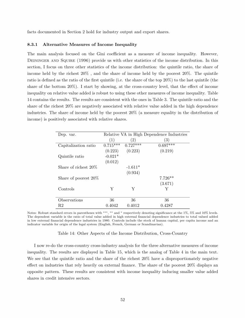
facts documented in Section 2 hold for industry output and export shares.

8.3.1 Alternative Measures of Income Inequality

The main analysis focused on the Gini coefficient as a measure of income inequality. However,Deininger and Squire (1996) provide us with other statistics of the income distribution. In thissection, I focus on three other statistics of the income distribution: the quintile ratio, the share ofincome held by the richest 20% , and the share of income held by the poorest 20%. The quintileratio is defined as the ratio of the first quintile (i.e. the share of the top 20%) to the last quintile (theshare of the bottom 20%). I start by showing, at the cross-country level, that the effect of incomeinequality on relative value added is robust to using these other measures of income inequality. Table14 contains the results. The results are consistent with the ones in Table 3. The quintile ratio and theshare of the richest 20% are negatively associated with relative value added in the high dependenceindustries. The share of income held by the poorest 20% (a measure equality in the distribution ofincome) is positively associated with relative shares.

Dep. var. Relative VA in High Dependence Industries(1) (2) (3)

Capitalization ratio 0.715*** 0.727*** 0.697***(0.223) (0.223) (0.219)

Quintile ratio -0.021*(0.012)

Share of richest 20% -1.611*(0.934)

Share of poorest 20% 7.726**(3.671)

Controls Y Y Y

Observations 36 36 36R2 0.4042 0.4012 0.4287

Notes: Robust standard errors in parentheses with ∗∗∗, ∗∗ and ∗ respectively denoting significance at the 1%, 5% and 10% levels.The dependent variable is the ratio of total value added in high external financial dependence industries to total valued addedin low external financial dependence industries in 1980. Controls include the stock of human capital, per capita income and anindicator variable for origin of the legal system (English, French, German or Scandinavian).

Table 14: Other Aspects of the Income Distribution, Cross-Country

I now re-do the cross-country cross-industry analysis for the three alternative measures of incomeinequality. The results are displayed in Table 15, which is the analog of Table 4 in the main text.We see that the quintile ratio and the share of the richest 20% have a disproportionately negativeeffect on industries that rely heavily on external finance. The share of the poorest 20% displays anopposite pattern. These results are consistent with income inequality inducing smaller value addedshares in credit intensive sectors.

52

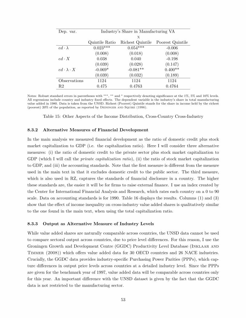
Dep. var. Industry’s Share in Manufacturing VAX

Quintile Ratio Richest Quintile Poorest Quintileed · λ 0.023*** 0.054*** -0.006

(0.008) (0.018) (0.008)ed ·X 0.038 0.040 -0.198

(0.039) (0.028) (0.147)ed · λ ·X -0.069* -0.081** 0.400**

(0.039) (0.032) (0.189)Observations 1124 1124 1124R2 0.475 0.4763 0.4764

Notes: Robust standard errors in parentheses with ∗∗∗, ∗∗ and ∗ respectively denoting significance at the 1%, 5% and 10% levels.All regressions include country and industry fixed effects. The dependent variable is the industry’s share in total manufacturingvalue added in 1980. Data is taken from the UNSD. Richest (Poorest) Quintile stands for the share in income held by the richest(poorest) 20% of the population, as reported by Deininger and Squire (1996).

Table 15: Other Aspects of the Income Distribution, Cross-Country Cross-Industry

8.3.2 Alternative Measures of Financial Development

In the main analysis we measured financial development as the ratio of domestic credit plus stockmarket capitalization to GDP (i.e. the capitalization ratio). Here I will consider three alternativemeasures: (i) the ratio of domestic credit to the private sector plus stock market capitalization toGDP (which I will call the private capitalization ratio), (ii) the ratio of stock market capitalizationto GDP, and (iii) the accounting standards. Note that the first measure is different from the measureused in the main text in that it excludes domestic credit to the public sector. The third measure,which is also used in RZ, captures the standards of financial disclosure in a country. The higherthese standards are, the easier it will be for firms to raise external finance. I use an index created bythe Center for International Financial Analysis and Research, which rates each country on a 0 to 90scale. Data on accounting standards is for 1990. Table 16 displays the results. Columns (1) and (3)show that the effect of income inequality on cross-industry value added shares is qualitatively similarto the one found in the main text, when using the total capitalization ratio.

8.3.3 Output as Alternative Measure of Industry Levels

While value added shares are naturally comparable across countries, the UNSD data cannot be usedto compare sectoral output across countries, due to price level differences. For this reason, I use theGroningen Growth and Development Centre (GGDC) Productivity Level Database (Inklaar andTimmer (2008)) which offers value added data for 30 OECD countries and 26 NACE industries.Crucially, the GGDC data provides industry-specific Purchasing Power Parities (PPPs), which cap-ture differences in output price levels across countries at a detailed industry level. Since the PPPsare given for the benchmark year of 1997, value added data will be comparable across countries onlyfor this year. An important difference with the UNSD dataset is given by the fact that the GGDCdata is not restricted to the manufacturing sector.

53

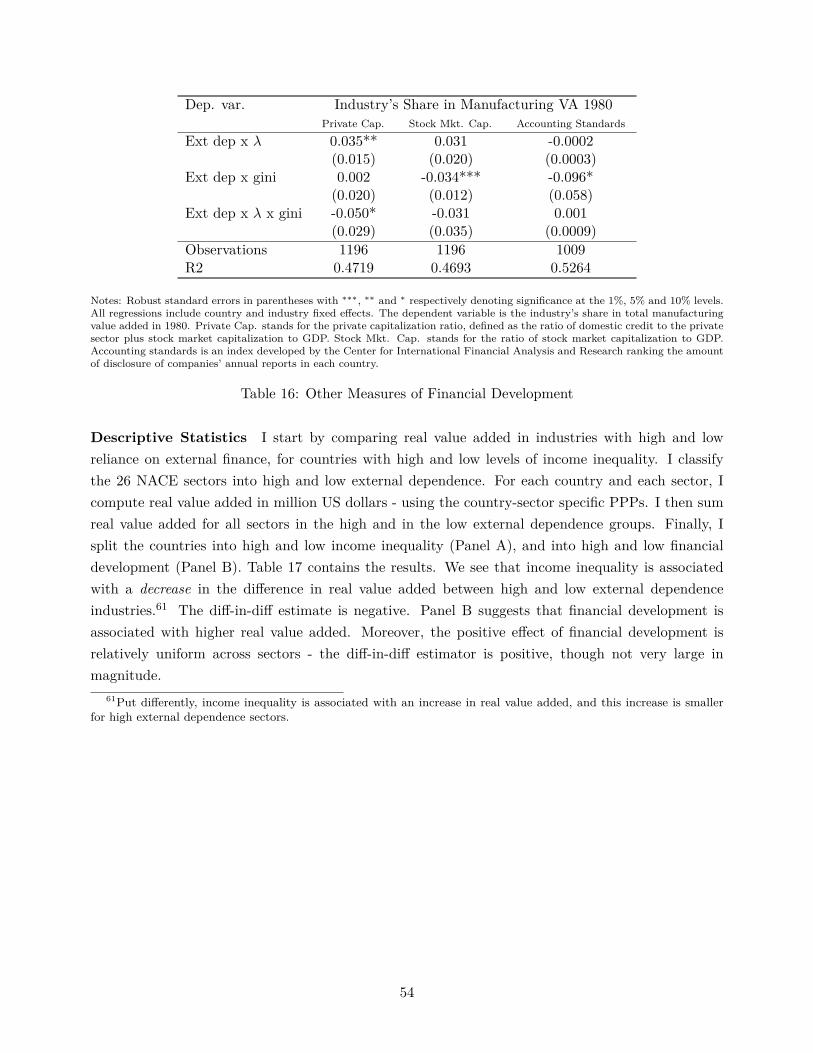
Dep. var. Industry’s Share in Manufacturing VA 1980Private Cap. Stock Mkt. Cap. Accounting Standards

Ext dep x λ 0.035** 0.031 -0.0002(0.015) (0.020) (0.0003)

Ext dep x gini 0.002 -0.034*** -0.096*(0.020) (0.012) (0.058)

Ext dep x λ x gini -0.050* -0.031 0.001(0.029) (0.035) (0.0009)

Observations 1196 1196 1009R2 0.4719 0.4693 0.5264

Notes: Robust standard errors in parentheses with ∗∗∗, ∗∗ and ∗ respectively denoting significance at the 1%, 5% and 10% levels.All regressions include country and industry fixed effects. The dependent variable is the industry’s share in total manufacturingvalue added in 1980. Private Cap. stands for the private capitalization ratio, defined as the ratio of domestic credit to the privatesector plus stock market capitalization to GDP. Stock Mkt. Cap. stands for the ratio of stock market capitalization to GDP.Accounting standards is an index developed by the Center for International Financial Analysis and Research ranking the amountof disclosure of companies’ annual reports in each country.

Table 16: Other Measures of Financial Development

Descriptive Statistics I start by comparing real value added in industries with high and lowreliance on external finance, for countries with high and low levels of income inequality. I classifythe 26 NACE sectors into high and low external dependence. For each country and each sector, Icompute real value added in million US dollars - using the country-sector specific PPPs. I then sumreal value added for all sectors in the high and in the low external dependence groups. Finally, Isplit the countries into high and low income inequality (Panel A), and into high and low financialdevelopment (Panel B). Table 17 contains the results. We see that income inequality is associatedwith a decrease in the difference in real value added between high and low external dependenceindustries.61 The diff-in-diff estimate is negative. Panel B suggests that financial development isassociated with higher real value added. Moreover, the positive effect of financial development isrelatively uniform across sectors - the diff-in-diff estimator is positive, though not very large inmagnitude.

61Put differently, income inequality is associated with an increase in real value added, and this increase is smallerfor high external dependence sectors.

54

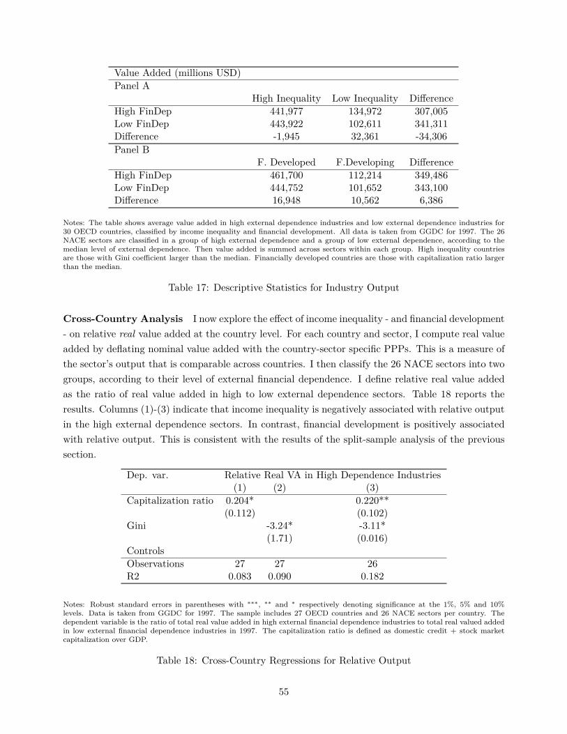
Value Added (millions USD)Panel A

High Inequality Low Inequality DifferenceHigh FinDep 441,977 134,972 307,005Low FinDep 443,922 102,611 341,311Difference -1,945 32,361 -34,306Panel B

F. Developed F.Developing DifferenceHigh FinDep 461,700 112,214 349,486Low FinDep 444,752 101,652 343,100Difference 16,948 10,562 6,386

Notes: The table shows average value added in high external dependence industries and low external dependence industries for30 OECD countries, classified by income inequality and financial development. All data is taken from GGDC for 1997. The 26NACE sectors are classified in a group of high external dependence and a group of low external dependence, according to themedian level of external dependence. Then value added is summed across sectors within each group. High inequality countriesare those with Gini coefficient larger than the median. Financially developed countries are those with capitalization ratio largerthan the median.

Table 17: Descriptive Statistics for Industry Output

Cross-Country Analysis I now explore the effect of income inequality - and financial development- on relative real value added at the country level. For each country and sector, I compute real valueadded by deflating nominal value added with the country-sector specific PPPs. This is a measure ofthe sector’s output that is comparable across countries. I then classify the 26 NACE sectors into twogroups, according to their level of external financial dependence. I define relative real value addedas the ratio of real value added in high to low external dependence sectors. Table 18 reports theresults. Columns (1)-(3) indicate that income inequality is negatively associated with relative outputin the high external dependence sectors. In contrast, financial development is positively associatedwith relative output. This is consistent with the results of the split-sample analysis of the previoussection.

Dep. var. Relative Real VA in High Dependence Industries(1) (2) (3)

Capitalization ratio 0.204* 0.220**(0.112) (0.102)

Gini -3.24* -3.11*(1.71) (0.016)

ControlsObservations 27 27 26R2 0.083 0.090 0.182

Notes: Robust standard errors in parentheses with ∗∗∗, ∗∗ and ∗ respectively denoting significance at the 1%, 5% and 10%levels. Data is taken from GGDC for 1997. The sample includes 27 OECD countries and 26 NACE sectors per country. Thedependent variable is the ratio of total real value added in high external financial dependence industries to total real valued addedin low external financial dependence industries in 1997. The capitalization ratio is defined as domestic credit + stock marketcapitalization over GDP.

Table 18: Cross-Country Regressions for Relative Output

55

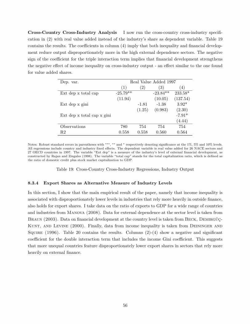
Cross-Country Cross-Industry Analysis I now run the cross-country cross-industry specifi-cation in (2) with real value added instead of the industry’s share as dependent variable. Table 19contains the results. The coefficients in column (4) imply that both inequality and financial develop-ment reduce output disproportionately more in the high external dependence sectors. The negativesign of the coefficient for the triple interaction term implies that financial development strengthensthe negative effect of income inequality on cross-industry output - an effect similar to the one foundfor value added shares.

Dep. var. Real Value Added 1997(1) (2) (3) (4)

Ext dep x total cap -25.79** -23.84** 233.58*(11.94) (10.05) (137.54)

Ext dep x gini -1.81 -1.38 3.92*(1.25) (0.983) (2.30)

Ext dep x total cap x gini -7.91*(4.44)

Observations 780 754 754 754R2 0.558 0.558 0.560 0.564

Notes: Robust standard errors in parentheses with ∗∗∗, ∗∗ and ∗ respectively denoting significance at the 1%, 5% and 10% levels.All regressions include country and industry fixed effects. The dependent variable is real value added for 26 NACE sectors and27 OECD countries in 1997. The variable “Ext dep” is a measure of the industry’s level of external financial development, asconstructed by Rajan and Zingales (1998). The variable “total cap” stands for the total capitalization ratio, which is defined asthe ratio of domestic credit plus stock market capitalization to GDP.

Table 19: Cross-Country Cross-Industry Regressions, Industry Output

8.3.4 Export Shares as Alternative Measure of Industry Levels

In this section, I show that the main empirical result of the paper, namely that income inequality isassociated with disproportionately lower levels in industries that rely more heavily in outside finance,also holds for export shares. I take data on the ratio of exports to GDP for a wide range of countriesand industries from Manova (2008). Data for external dependence at the sector level is taken fromBraun (2003). Data on financial development at the country level is taken from Beck, Demirgüç-Kunt, and Levine (2000). Finally, data from income inequality is taken from Deininger andSquire (1996). Table 20 contains the results. Columns (2)-(4) show a negative and significantcoefficient for the double interaction term that includes the income Gini coefficient. This suggeststhat more unequal countries feature disproportionately lower export shares in sectors that rely moreheavily on external finance.

56

Dep. var. Industry’s Average Export Share 1980-1997

(1) (2) (3) (4)Ext dep x total cap 0.795*** 0.646*** 0.848

(0.187) (0.1908) (1.038)Ext dep x gini -6.191*** -4.619*** -4.239*

(1.207) (1.143) (2.255)Ext dep x total cap x gini -0.482

(2.346)Observations 1134 1161 1134 1134R2 0.7153 0.7112 0.7186 0.7186

Notes: Robust standard errors in parentheses with ∗∗∗, ∗∗ and ∗ respectively denoting significance at the 1%, 5% and 10% levels.All regressions include country and industry fixed effects. The dependent variable is the industry’s export share averaged over theperiod 1980-1997, taken from Manova (2008). The variable “Ext dep” is a measure of the industry’s level of external financialdevelopment, as constructed by Braun (2003). The variable “total cap” stands for the total capitalization ratio, which is definedas the ratio of domestic credit plus stock market capitalization to GDP. The coefficients estimates and standard errors of anyterm that includes the Gini coefficient were multiplied by 100.

Table 20: Cross-Country Cross-Industry Regressions for Exports

8.4 First Best Equilibrium

In this subsection, I outline the equilibrium conditions for the perfect credit benchmark (that is,the economy with λ = ∞). In this case, all agents achieve the optimal scale of production, andpersonal wealth is irrelevant for production decisions. Thus, every agent is indifferent between thedifferent sectors and occupations. An equilibrium now consists of prices (p1, p2, r, w), a mass of agentsallocated to sector 1, µ, and a mass of workers, µ0, such that:

57

1. Indifference:

(1− ν)(p1A1ν

ν(

α

r + δ

)αν (1− αw

)(1−α)ν) 1

1−ν

= (1− ν)(p2A2ν

ν(

α

r + δ

)αν (1− αw

)(1−α)ν) 1

1−ν

−(r+δ)f

(23)= w

2. Capital market clearing:

µ

(p1A1ν

(1− αw

)ν(1−α) ( α

r + δ

)1−ν(1−α)) 1

1−ν

+(1− µ− µ0)

(p2A2ν

(1− αw

)ν(1−α) ( α

r + δ

)1−ν(1−α)) 1

1−ν

+ f

(24)

= E [ω]

3. Labor market clearing:

µ

(p1A1ν

(1− αw

)1−αν ( α

r + δ

)αν) 11−ν

+(1− µ− µ0)(p2A2ν

(1− αw

)1−αν ( α

r + δ

)αν) 11−ν

= µ0

(25)

4. Final good optimality:

µ (p1A1)1

1−ν =(

γ

1− γp2p1

)ε(1− µ− µ0) (p2A2)

11−ν (26)

5. Free entry into final good sector:

[γεp1−ε

1 + (1− γ)ε p1−ε2

] 11−ε = 1 (27)

8.5 US Distribution of Wealth and the Pareto Assumption

In this section, I show that the Pareto distribution is a good approximation of the upper tail of thewealth distribution. Figure 20 shows an histogram of the distribution of wealth among US householdsfor 1983. Data is taken from the Survey of Consumer Finances. The figure shows households withwealth greater than $95,000 - which represents 25% of the population. The figure also shows a Paretodensity with shape parameter as the one assumed in the main text. We see that the Pareto densityis close to the population histogram.

58

Density

100000 200000 300000 400000 500000Wealth

Notes: Data from the US Survey of Consumer Finances for 1983. The histogram shows data for households with wealth between$95,000 and $500,000. Both the normal and the high income sample are included. Wealth (net worth) is given by variable B3324,which is defined as.gross assets excluding pensions plus total net present value of pensions minus total debt (B3305 + B3316 -B3320). The solid line corresponds to the density of a Pareto distribution, with scale parameter $95,000 and shape parameterequal to 1.1412.

Figure 20: Upper Tail of Wealth Distribution

I also perform a maximum likelihood fit of the Pareto distribution for wealth levels above $95,000,and find an estimated shape parameter of 1.13. The value found in the calibration done in the maintext was 1.14.

8.6 Sensitivity Analysis

Figure 21 considers the case in which the fixed cost is higher (f=$200,000 instead of $55,280). Therest of the parameters are kept at the values used in Section 6.1. I find that in this case the losses fromwealth inequality are substantially smaller than in the baseline case with smaller fixed cost. First,for initially low values of inequality, a mean preserving spread can lead to higher output. Second,considering the full range of inequality values, output falls by about 18 percent, i.e. a substantiallysmaller loss than in the baseline model of the main text. These results are consistent with thediscussion of the extensive margin channel in Section 3.3.

59

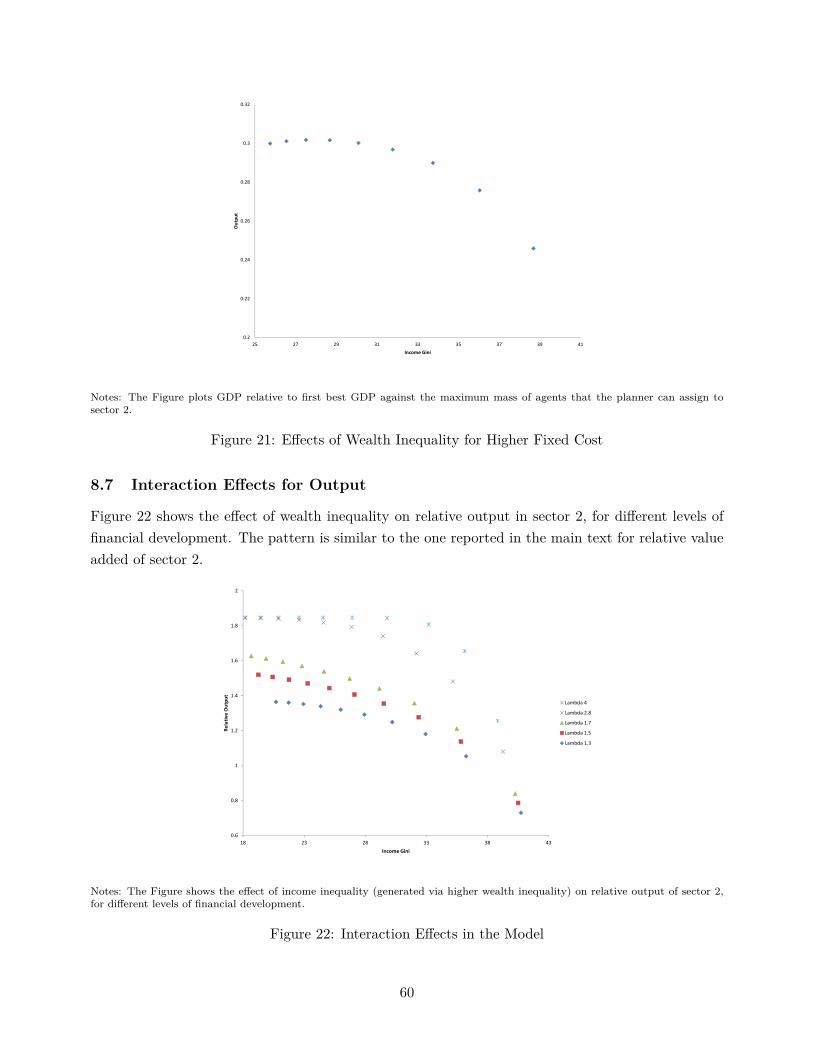
0.26

0.28

0.3

0.32

Ou

tpu

t

0.2

0.22

0.24

25 27 29 31 33 35 37 39 41

Income Gini

Notes: The Figure plots GDP relative to first best GDP against the maximum mass of agents that the planner can assign tosector 2.

Figure 21: Effects of Wealth Inequality for Higher Fixed Cost

8.7 Interaction Effects for Output

Figure 22 shows the effect of wealth inequality on relative output in sector 2, for different levels offinancial development. The pattern is similar to the one reported in the main text for relative valueadded of sector 2.

1.2

1.4

1.6

1.8

2

Re

lati

ve

Ou

tpu

t

Lambda 4

Lambda 2.8

Lambda 1.7

Lambda 1.5

Lambda 1.3

0.6

0.8

1

18 23 28 33 38 43

Income Gini

Lambda 1.3

Notes: The Figure shows the effect of income inequality (generated via higher wealth inequality) on relative output of sector 2,for different levels of financial development.

Figure 22: Interaction Effects in the Model

60

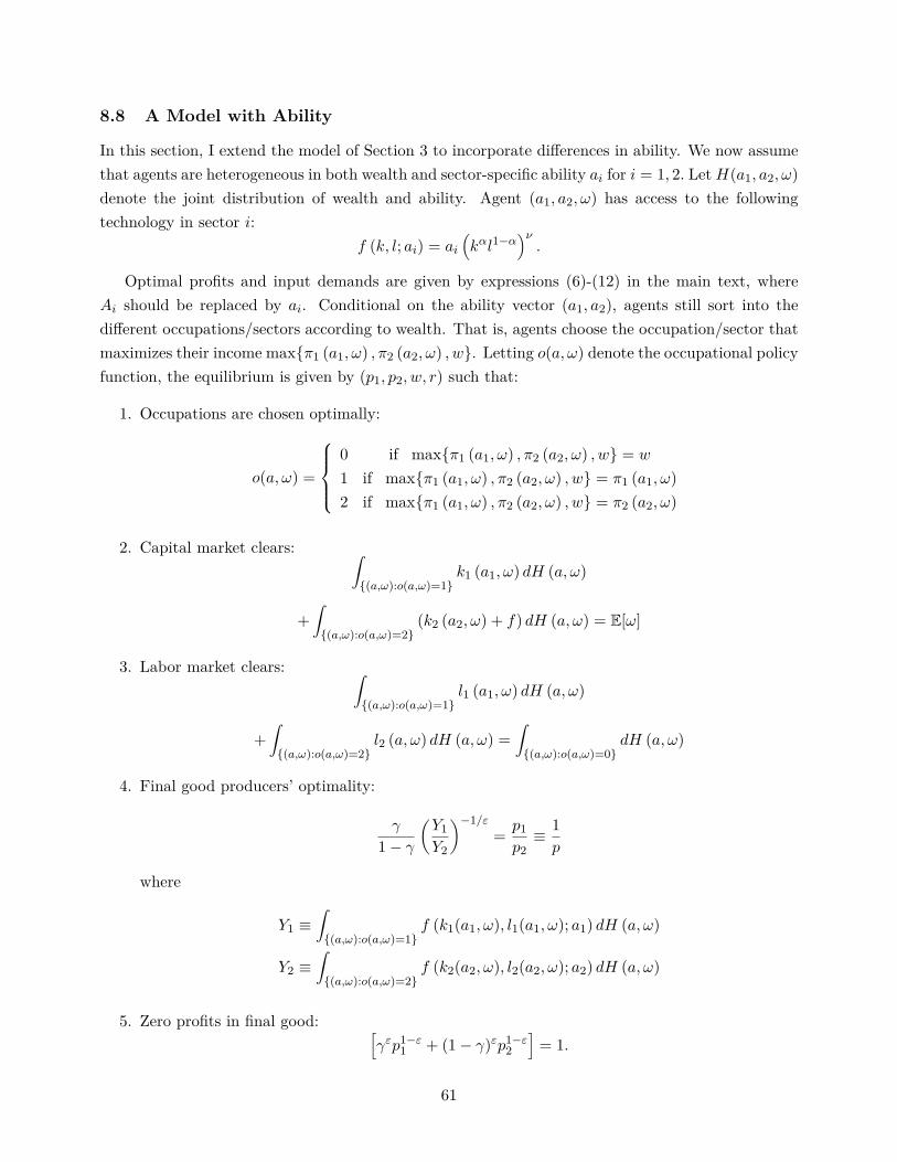
8.8 A Model with Ability

In this section, I extend the model of Section 3 to incorporate differences in ability. We now assumethat agents are heterogeneous in both wealth and sector-specific ability ai for i = 1, 2. LetH(a1, a2, ω)denote the joint distribution of wealth and ability. Agent (a1, a2, ω) has access to the followingtechnology in sector i:

f (k, l; ai) = ai(kαl1−α

)ν.

Optimal profits and input demands are given by expressions (6)-(12) in the main text, whereAi should be replaced by ai. Conditional on the ability vector (a1, a2), agents still sort into thedifferent occupations/sectors according to wealth. That is, agents choose the occupation/sector thatmaximizes their income max{π1 (a1, ω) , π2 (a2, ω) , w}. Letting o(a, ω) denote the occupational policyfunction, the equilibrium is given by (p1, p2, w, r) such that:

1. Occupations are chosen optimally:

o(a, ω) =

0 if max{π1 (a1, ω) , π2 (a2, ω) , w} = w

1 if max{π1 (a1, ω) , π2 (a2, ω) , w} = π1 (a1, ω)2 if max{π1 (a1, ω) , π2 (a2, ω) , w} = π2 (a2, ω)

2. Capital market clears: ∫{(a,ω):o(a,ω)=1}

k1 (a1, ω) dH (a, ω)

+∫{(a,ω):o(a,ω)=2}

(k2 (a2, ω) + f) dH (a, ω) = E[ω]

3. Labor market clears: ∫{(a,ω):o(a,ω)=1}

l1 (a1, ω) dH (a, ω)

+∫{(a,ω):o(a,ω)=2}

l2 (a, ω) dH (a, ω) =∫{(a,ω):o(a,ω)=0}

dH (a, ω)

4. Final good producers’ optimality:

γ

1− γ

(Y1Y2

)−1/ε= p1p2≡ 1p

where

Y1 ≡∫{(a,ω):o(a,ω)=1}

f (k1(a1, ω), l1(a1, ω); a1) dH (a, ω)

Y2 ≡∫{(a,ω):o(a,ω)=2}

f (k2(a2, ω), l2(a2, ω); a2) dH (a, ω)

5. Zero profits in final good: [γεp1−ε

1 + (1− γ)εp1−ε2

]= 1.

61

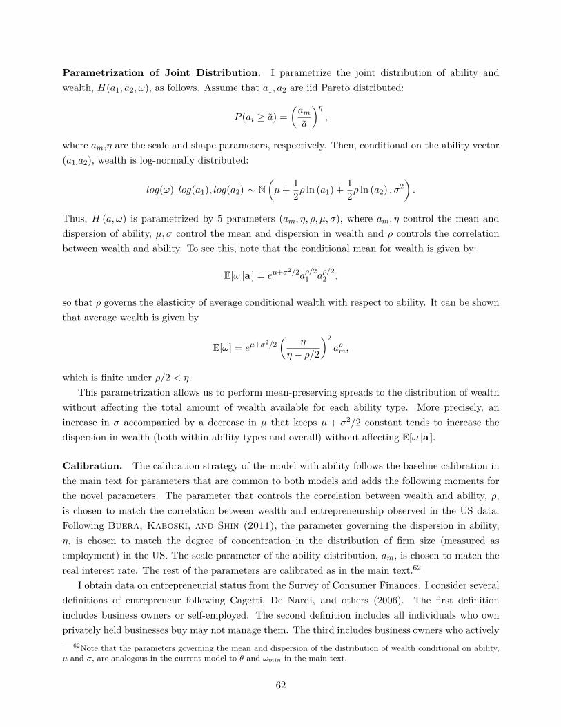
Parametrization of Joint Distribution. I parametrize the joint distribution of ability andwealth, H(a1, a2, ω), as follows. Assume that a1, a2 are iid Pareto distributed:

P (ai ≥ a) =(ama

)η,

where am,η are the scale and shape parameters, respectively. Then, conditional on the ability vector(a1,a2), wealth is log-normally distributed:

log(ω) |log(a1), log(a2) ∼ N(µ+ 1

2ρ ln (a1) + 12ρ ln (a2) , σ2

).

Thus, H (a, ω) is parametrized by 5 parameters (am, η, ρ, µ, σ), where am, η control the mean anddispersion of ability, µ, σ control the mean and dispersion in wealth and ρ controls the correlationbetween wealth and ability. To see this, note that the conditional mean for wealth is given by:

E[ω |a ] = eµ+σ2/2aρ/21 a

ρ/22 ,

so that ρ governs the elasticity of average conditional wealth with respect to ability. It can be shownthat average wealth is given by

E[ω] = eµ+σ2/2(

η

η − ρ/2

)2aρm,

which is finite under ρ/2 < η.

This parametrization allows us to perform mean-preserving spreads to the distribution of wealthwithout affecting the total amount of wealth available for each ability type. More precisely, anincrease in σ accompanied by a decrease in µ that keeps µ + σ2/2 constant tends to increase thedispersion in wealth (both within ability types and overall) without affecting E[ω |a ].

Calibration. The calibration strategy of the model with ability follows the baseline calibration inthe main text for parameters that are common to both models and adds the following moments forthe novel parameters. The parameter that controls the correlation between wealth and ability, ρ,is chosen to match the correlation between wealth and entrepreneurship observed in the US data.Following Buera, Kaboski, and Shin (2011), the parameter governing the dispersion in ability,η, is chosen to match the degree of concentration in the distribution of firm size (measured asemployment) in the US. The scale parameter of the ability distribution, am, is chosen to match thereal interest rate. The rest of the parameters are calibrated as in the main text.62

I obtain data on entrepreneurial status from the Survey of Consumer Finances. I consider severaldefinitions of entrepreneur following Cagetti, De Nardi, and others (2006). The first definitionincludes business owners or self-employed. The second definition includes all individuals who ownprivately held businesses buy may not manage them. The third includes business owners who actively

62Note that the parameters governing the mean and dispersion of the distribution of wealth conditional on ability,µ and σ, are analogous in the current model to θ and ωmin in the main text.

62

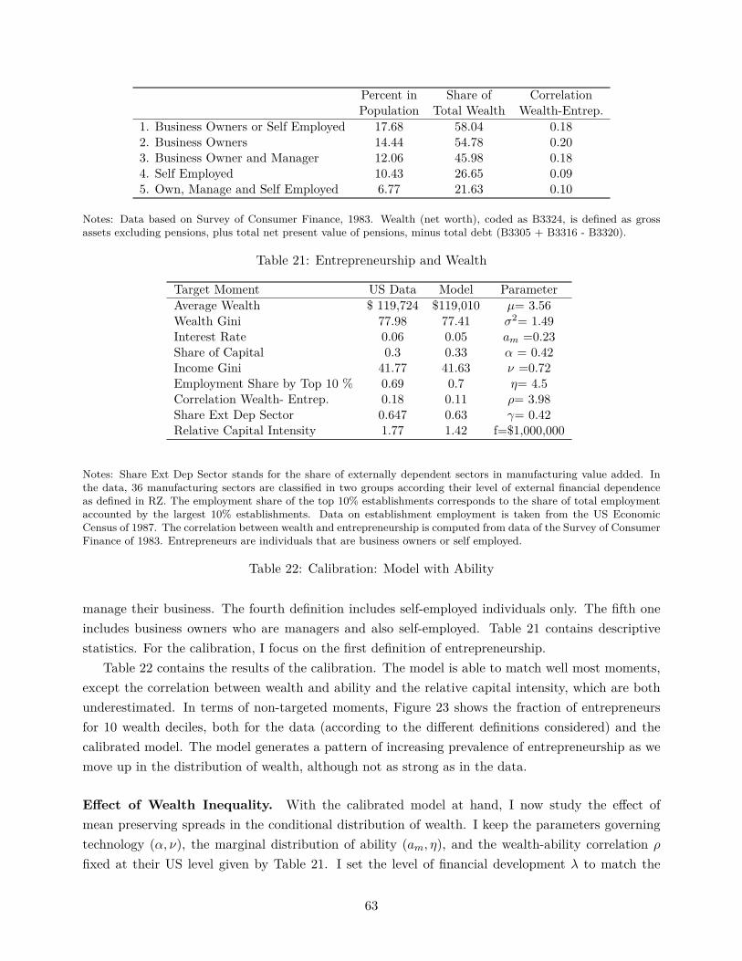
Percent in Share of CorrelationPopulation Total Wealth Wealth-Entrep.

1. Business Owners or Self Employed 17.68 58.04 0.182. Business Owners 14.44 54.78 0.203. Business Owner and Manager 12.06 45.98 0.184. Self Employed 10.43 26.65 0.095. Own, Manage and Self Employed 6.77 21.63 0.10

Notes: Data based on Survey of Consumer Finance, 1983. Wealth (net worth), coded as B3324, is defined as grossassets excluding pensions, plus total net present value of pensions, minus total debt (B3305 + B3316 - B3320).

Table 21: Entrepreneurship and Wealth

Target Moment US Data Model ParameterAverage Wealth $ 119,724 $119,010 µ= 3.56Wealth Gini 77.98 77.41 σ2= 1.49Interest Rate 0.06 0.05 am =0.23Share of Capital 0.3 0.33 α = 0.42Income Gini 41.77 41.63 ν =0.72Employment Share by Top 10 % 0.69 0.7 η= 4.5Correlation Wealth- Entrep. 0.18 0.11 ρ= 3.98Share Ext Dep Sector 0.647 0.63 γ= 0.42Relative Capital Intensity 1.77 1.42 f=$1,000,000

Notes: Share Ext Dep Sector stands for the share of externally dependent sectors in manufacturing value added. Inthe data, 36 manufacturing sectors are classified in two groups according their level of external financial dependenceas defined in RZ. The employment share of the top 10% establishments corresponds to the share of total employmentaccounted by the largest 10% establishments. Data on establishment employment is taken from the US EconomicCensus of 1987. The correlation between wealth and entrepreneurship is computed from data of the Survey of ConsumerFinance of 1983. Entrepreneurs are individuals that are business owners or self employed.

Table 22: Calibration: Model with Ability

manage their business. The fourth definition includes self-employed individuals only. The fifth oneincludes business owners who are managers and also self-employed. Table 21 contains descriptivestatistics. For the calibration, I focus on the first definition of entrepreneurship.

Table 22 contains the results of the calibration. The model is able to match well most moments,except the correlation between wealth and ability and the relative capital intensity, which are bothunderestimated. In terms of non-targeted moments, Figure 23 shows the fraction of entrepreneursfor 10 wealth deciles, both for the data (according to the different definitions considered) and thecalibrated model. The model generates a pattern of increasing prevalence of entrepreneurship as wemove up in the distribution of wealth, although not as strong as in the data.

Effect of Wealth Inequality. With the calibrated model at hand, I now study the effect ofmean preserving spreads in the conditional distribution of wealth. I keep the parameters governingtechnology (α, ν), the marginal distribution of ability (am, η), and the wealth-ability correlation ρ

fixed at their US level given by Table 21. I set the level of financial development λ to match the

63

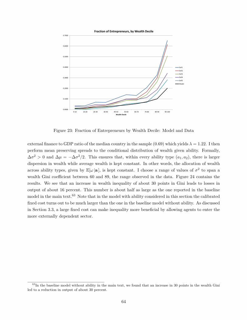
0.0000

0.1000

0.2000

0.3000

0.4000

0.5000

0.6000

0.7000

0‐10 10‐20 20‐30 30‐40 40‐50 50‐60 60‐70 70‐80 80‐90 90‐100Wealth Decile

Fraction of Entrepreneurs, by Wealth Decile

Def1

Def2

Def3

Def4

Def5

Model

Figure 23: Fraction of Entrepreneurs by Wealth Decile: Model and Data

external finance to GDP ratio of the median country in the sample (0.69) which yields λ = 1.22. I thenperform mean preserving spreads to the conditional distribution of wealth given ability. Formally,∆σ2 > 0 and ∆µ = −∆σ2/2. This ensures that, within every ability type (a1, a2), there is largerdispersion in wealth while average wealth is kept constant. In other words, the allocation of wealthacross ability types, given by E[ω |a ], is kept constant. I choose a range of values of σ2 to span awealth Gini coefficient between 60 and 89, the range observed in the data. Figure 24 contains theresults. We see that an increase in wealth inequality of about 30 points in Gini leads to losses inoutput of about 16 percent. This number is about half as large as the one reported in the baselinemodel in the main text.63 Note that in the model with ability considered in this section the calibratedfixed cost turns out to be much larger than the one in the baseline model without ability. As discussedin Section 3.3, a large fixed cost can make inequality more beneficial by allowing agents to enter themore externally dependent sector.

63In the baseline model without ability in the main text, we found that an increase in 30 points in the wealth Giniled to a reduction in output of about 30 percent.

64

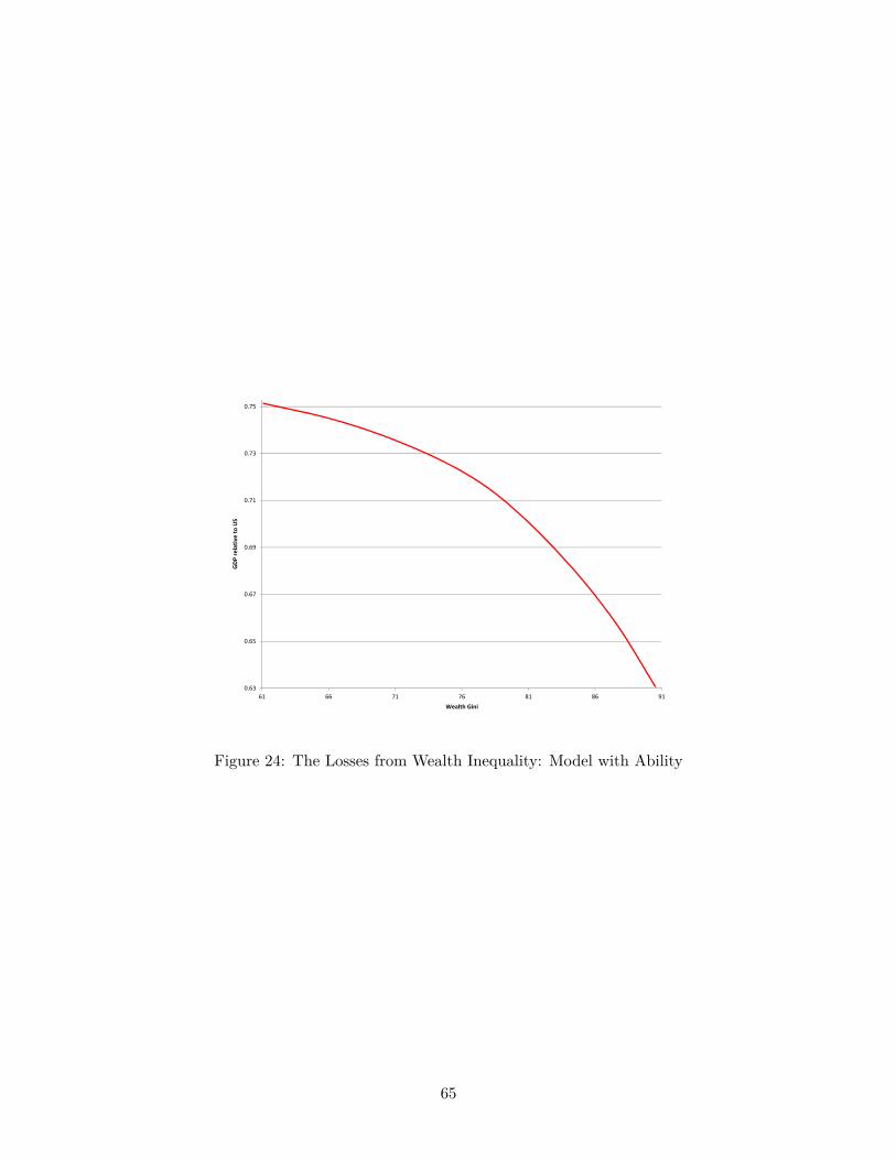
0.63

0.65

0.67

0.69

0.71

0.73

0.75

61 66 71 76 81 86 91

GDP relativ

e to US

Wealth Gini

Figure 24: The Losses from Wealth Inequality: Model with Ability

65