econstor www.econstor.eu

Der Open-Access-Publikationsserver der ZBW – Leibniz-Informationszentrum WirtschaftThe Open Access Publication Server of the ZBW – Leibniz Information Centre for Economics

Standard-Nutzungsbedingungen:

Die Dokumente auf EconStor dürfen zu eigenen wissenschaftlichenZwecken und zum Privatgebrauch gespeichert und kopiert werden.

Sie dürfen die Dokumente nicht für öffentliche oder kommerzielleZwecke vervielfältigen, öffentlich ausstellen, öffentlich zugänglichmachen, vertreiben oder anderweitig nutzen.

Sofern die Verfasser die Dokumente unter Open-Content-Lizenzen(insbesondere CC-Lizenzen) zur Verfügung gestellt haben sollten,gelten abweichend von diesen Nutzungsbedingungen die in der dortgenannten Lizenz gewährten Nutzungsrechte.

Terms of use:

Documents in EconStor may be saved and copied for yourpersonal and scholarly purposes.

You are not to copy documents for public or commercialpurposes, to exhibit the documents publicly, to make thempublicly available on the internet, or to distribute or otherwiseuse the documents in public.

If the documents have been made available under an OpenContent Licence (especially Creative Commons Licences), youmay exercise further usage rights as specified in the indicatedlicence.

zbw Leibniz-Informationszentrum WirtschaftLeibniz Information Centre for Economics

Hoffmann, Mathias; Suter, Rahel

Working Paper

Systematic Consumption Risk in Currency Returns

CESifo Working Paper, No. 4273

Provided in Cooperation with:Ifo Institute – Leibniz Institute for Economic Research at the University ofMunich

Suggested Citation: Hoffmann, Mathias; Suter, Rahel (2013) : Systematic Consumption Risk inCurrency Returns, CESifo Working Paper, No. 4273

This Version is available at:http://hdl.handle.net/10419/77705

Systematic Consumption Risk in Currency Returns

Mathias Hoffmann Rahel Suter

CESIFO WORKING PAPER NO. 4273 CATEGORY 7: MONETARY POLICY AND INTERNATIONAL FINANCE

JUNE 2013

Presented at CESifo Area Conference on Macro, Money & International Finance, February 2013

An electronic version of the paper may be downloaded • from the SSRN website: www.SSRN.com • from the RePEc website: www.RePEc.org

• from the CESifo website: Twww.CESifo-group.org/wp T

CESifo Working Paper No. 4273

Systematic Consumption Risk in Currency Returns

Abstract We sort currencies by countries’ consumption growth over the past four quarters. Currency portfolios of countries experiencing consumption booms have higher Sharpe ratios than those of countries going through a consumption-based recession. A carry strategy that goes short in countries that are in a consumption bust and goes long in countries with a consumption boom yields consistently positive excess returns. This excess return compensates for the risk of high negative returns in worldwide downturns. Our consumption carry factor prices the cross section of portfolios of currencies sorted on various characteristics (consumption, interest rates) and also does well on the cross section of bilateral currency movements. Eventually, a habit formation model allows to interpret these results: sorting currencies on past consumption growth is akin to sorting countries on risk aversion, and low (high) risk aversion currencies depreciate (appreciate) in times of global turmoil.

JEL-Code: E440, F310, F440, G120, G150.

Keywords: foreign exchange, carry trade returns, consumption risk, asset pricing.

Mathias Hoffmann University of Zurich

Department of Economics, International Trade & Finance Group Zuerichbergstrasse 14

Switzerland – 8032 Zurich mathias.hoffmann@econ.uzh.ch

Rahel Suter University of Zurich

Department of Economics, International Trade & Finance Group Zuerichbergstrasse 14

Switzerland – 8032 Zurich rahel.suter@econ.uzh.ch

May 2013 We would like to thank Adrien Verdelhan and Angelo Ranaldo for very helpful discussions and comments. We are also grateful to seminar participants at the University of Zurich and at the CESifo Money Macro and Finance Conference 2013 in Munich.

1 Introduction

In this paper, we provide evidence that currency returns reflect cross-country differences in

consumption risk. We do so by sorting currencies into portfolios based on countries’ consump-

tion growth over the last four quarters. Currencies of countries that have experienced high

consumption growth (relative to the world median) have consistently higher Sharpe ratios than

currencies in the lower half of the consumption-growth distribution. A consumption carry fac-

tor that reflects the return of going short on currencies of low-consumption-growth (‘consump-

tion bust’) countries and long on the currencies of consumption boom countries explains the

cross section of currency returns in our sample of 33 countries over the period 1990− 2010. We

call this factor the consumption carry factor and denote it by HML∆c.

In recent years, the idea that movements in currency prices can be explained by the trade-off

between risk and return has gained renewed attention and considerable empirical support. At

a general level, a couple of conditions need to be fulfilled for currency returns to reflect a com-

pensation for some form of macroeconomic or financial risk. First, currencies that pay high

returns on average must perform relatively badly in bad times, whereas currencies that pay

low returns on average must perform well in bad times. Second, currency returns must reflect

cross-country differences in the exposure to common (global) risk, because only global risk will

be priced in integrated world capital markets. Lustig et al. (2011) show that currency returns

are well explained by a two-factor model in which the first factor is the average return on the

dollar vis-a-vis all other currencies, and the second factor is the spread in returns between a

portfolio of high-interest-rate currencies and a portfolio of low- interest-rate currencies. As the

latter factor, which is a carry trade factor and denoted HMLFX, pays off badly in crises, dif-

ferences in the exposure of high- and low-interest-rate currencies to this factor can explain a

substantial fraction of the variation in the cross section of interest-rate-sorted currency port-

folios. Verdelhan (2011) extends this framework to the pricing of bilateral exchange rates and

argues that differences in the exposure to a (level) dollar factor are also a key element of the

systematic variation in exchange rates. Ranaldo and Soderlind (2010) find that so-called ‘safe

haven’ currencies pay relatively high returns precisely when foreign exchange market volatil-

ity increases, whereas the returns from ‘investment currencies’ are low in times of high foreign

exchange market turbulences. Menkhoff et al. (2012) add to these findings by showing that a

2

foreign exchange volatility innovation factor rationalizes the spread in returns of interest-rate-

sorted currency portfolios. Together, all these results suggest that the returns obtained from

holding particular currencies or currency portfolios compensate an investor for global market

risk.

While these studies provide compelling evidence for a risk–return trade-off in foreign exchange

markets, they propose financial factors as an explanation for currency returns. Hence, they do

not fully address the extent to which these risk factors truly reflect macroeconomic and, in

particular, consumption risk. Another strand of the literature has recently begun to address

this issue. For example, Lustig and Verdelhan (2007) argue that an extended version of the

consumption-based capital asset pricing model (C-CAPM) with Epstein–Zin preferences and a

durable consumption good can explain the cross section of interest-rate-sorted currency port-

folios. Colacito and Croce (2011) show that a version of the long-run risk model by Bansal

and Yaron (2004) explains currency movements quite well, and Verdelhan (2010) shows that

consumption habits can explain the cross section of currency returns.

The analysis in this paper positions itself between these two strands of the literature. We fol-

low the first strand and construct a simple pricing factor that is based on sorting currencies into

portfolios according to ex ante observable characteristics. This approach allows us to discuss

the determinants of currency returns under as few theoretical assumptions as possible — in

particular, we do not specify restrictions on preferences. We follow the second strand of the lit-

erature, however, by focusing on consumption fluctuations as a driver of variation in currency

returns. Linking these two approaches allows us to determine the structure of consumption risk

priced into currencies directly from the data without having to confront the particular moment

restrictions that specific versions of the consumption-based asset pricing model may impose

on the data. In a last step, we relate our results back to the consumption-based literature by

interpreting them in the context of a consumption-based model with habit formation.

We sort currencies into portfolios based on countries’ past consumption growth. Currencies of

countries with higher past consumption growth consistently pay higher returns than currencies

of countries with low consumption growth, and the spread in these returns is well explained

by the consumption carry factor HML∆c, which equals the difference in returns of the high and

the low-consumption-growth currency portfolios.

3

Our consumption carry factor HML∆c is constructed in analogy to the HMLFX factor proposed

by Lustig et al. (2011), and it has a number of interesting properties. For example, even though

our HML∆c factor is correlated with the Lustig et al. (2011) HMLFX factor, the two are clearly

not the same variable. In particular, the consumption-based carry strategy did a lot better than

the interest-rate-based carry strategy during the recent financial crisis. In fact, returns from

the consumption factor HML∆c are much less skewed than returns from the interest carry fac-

tor HMLFX and generate a lower Sharpe ratio. In a direct comparison of its ability to price

exchange rates, the consumption carry factor HML∆c compares favorably with other financial

risk factors that have recently been proposed in the literature. In particular, it is also success-

ful in pricing the interest-rate-sorted currency portfolios used elsewhere in the literature. In

addition, we show that HML∆c also prices individual currencies.

While we emphasize that our empirical results are obtained without recourse to a particular

consumption-based asset pricing model, we conclude by linking them back to economic the-

ory. Specifically, we suggest that they be interpreted within the framework of a consumption-

based model with habit formation in the mold of Campbell and Cochrane (1999) and Verdelhan

(2010).

In a model with habit formation, sorting currencies on past consumption growth amounts to

sorting countries by their surplus consumption ratio and, therefore, by their degree of risk

aversion. Marginal utility in high-risk-aversion countries is more sensitive to global consump-

tion shocks than in low- risk-aversion countries, and optimal risk sharing requires currencies of

countries with high (low) risk aversion to appreciate (depreciate) in times of global downturns.

The risk of a large depreciation when consumption growth suddenly drops is the risk that in-

vestors get compensated for by high average returns that currencies with high past consump-

tion growth pay. In the habit model, our HML∆c factor reflects the spread between the return

of low- and high-risk-aversion currencies, which implies that it must turn low in bad times.

We show that a realistically calibrated version of the habit model with a global consumption

growth shock can broadly replicate the empirical findings that we present in the main part of

the paper.

Our results and analysis also connect to the macroeconomic literature on the role of exchange

rates in international consumption risk sharing. Early models in this literature (Backus and

4

Smith (1993) and Kollmann (1995)) assume standard constant relative risk aversion preferences.

In these models, differences in consumption growth between countries are the only driver of

differences in marginal utility growth between countries. If financial markets are complete,

real exchange rate changes should therefore be perfectly correlated with consumption growth

differences between countries. In the data, however, correlations between consumption and

real exchange rates tend to be low, suggesting low levels of international risk sharing. The

results in this paper shed new light on the structure of the consumption–real-exchange-rate

anomaly: our finding is that countries with high (past) consumption growth tend to have ap-

preciating currencies.1 The habit model can explain this specific pattern because it allows coun-

tries’ marginal utility to differ even if there are no differences in consumption growth at a given

point in time: because of habit formation, past differences in consumption growth will drive

marginal utility of today’s consumption down in high-consumption growth economies and up

in low-consumption growth economies. Optimal risk sharing therefore requires the former to

depreciate in response to a global consumption shock.

The paper is organized as follows. The next section further connects our empirical approach

and the previous literature. Section 3 defines currency returns and discusses the formation

of portfolios based on past consumption growth. Section 4 describes the data set used in the

empirical analysis, and Section 5 presents the empirical results. In Section 6, we interpret our

empirical results in the context of a version of the Campbell and Cochrane (1999) habit model.

Section 7 presents an overview of some robustness checks, and Section 8 concludes.

2 Related literature

Starting with Fama (1984), a large literature has documented the resounding rejection of un-

covered interest parity (UIP) in the data. In fact, there is considerable structure in this rejection:

currencies of countries with high interest rates do not depreciate as much as would be implied

by UIP. This UIP puzzle, along with the finding by Meese and Rogoff (1983) that exchange

rates are hard to predict out-of-sample, gave rise to a large empirical literature on exchange

rate modeling. It is probably fair to say that much of this early literature was rather skeptical1Note that this pattern is quite reminiscent of the uncovered interest parity (UIP) puzzle that consists of the

observation that high-interest- rate currencies do not depreciate as much as UIP would predict and that they oftenwill actually appreciate.

5

with respect to risk-based explanations of currency returns. Engel (1996) and Lewis (1995) pro-

vide useful surveys. During the last decade, the notion that currency returns, just like those of

other assets, could be determined by risk premia has gained renewed attention and — proba-

bly because of the availability of more, better and larger data sets and theoretical advances in

asset pricing theory — is continuing to gather empirical support.

A valid explanation of the UIP puzzle in terms of risk premia would require that investment

in currencies with high interest rates — which promise high returns on average — would de-

liver especially low returns in bad times for investors. If this was the case, carry trade profits

would just compensate an investor for risk that he exposes himself to when holding particu-

lar currencies. Empirically, however, it is challenging to identify risk factors, and especially

macroeconomic risk factors, that would drive currency risk premia.2 In this respect, an impor-

tant contribution is the study by Lustig and Verdelhan (2007). As interest rates seem to predict

currency returns, Lustig and Verdelhan sorted a wide cross section of currencies into portfolios

according to their interest rate differentials with the US. Portfolios are rebalanced every pe-

riod such that the first portfolio always contains the lowest-interest-rate currencies and the last

portfolio always contains the highest-interest-rate currencies. Sorting currencies into portfolios

eliminates diversifiable, currency-specific components of returns such that sharp estimates of

the risk–return tradeoff of currency investments are obtained. Eventually, Lustig and Verdel-

han (2007) show within the framework of consumption-based capital asset pricing models that

the growth rate of durable and nondurable consumption expenditures, as well as the mean

return of the US stock market, are helpful in explaining currency portfolio returns.

In a subsequent study, using a data-driven approach in the spirit of Fama and French (1993),

Lustig et al. (2011) find that the currency portfolios themselves contain information to explain

the cross section of portfolio returns. Lustig et al. (2011) identify two factors that together ac-

count for most of the variability in the cross section of currency portfolio returns. The first

factor, which they coin the ‘dollar risk factor’, is the average return that an investor gains by

borrowing in US dollars and investing in equal weights in all currencies available. This dollar-

specific factor acts as a level factor for portfolio returns. The second factor equals the return

that a global investor gains by going short in the low-interest-rate currency portfolio and long

2Burnside et al. (2011) find that traditional risk factors do not explain currency returns, instead attributing theforward premium to peso problems.

6

in the high-interest-rate currency portfolio. Lustig et al. (2011) denote this carry trade factor

HMLFX. While profitable for most of the time, such a carry trade strategy yields low returns

during times of global turmoil, which implies a negative HMLFX factor. As expected returns

increase monotonically from low- to high-interest- rate currency portfolios, and because the

covariation of portfolio returns and HMLFX is higher, the higher the interest rates of a partic-

ular currency portfolio are, the more HMLFX qualifies as a slope factor for currency portfolio

returns. Closely related to these results, the study by Menkhoff et al. (2012) concludes that a

factor that measures news in global foreign exchange market volatility decisively explains the

returns to carry trades. High expected carry trade returns can be rationalized within standard

asset pricing models, because these returns turn especially low during times of high foreign ex-

change market volatility surprises when investors particularly fear losses. Brunnermeier et al.

(2008) uncover another link between the performance of carry trades and market volatility. Ac-

cording to their reasoning, a sudden increase in stock market volatility (as measured by the

CBOE’s VIX) could cause a decrease in risk appetite and funding liquidity, which then makes

investors unwind their carry trades. An orchestrated sellout of investment currencies depre-

ciates their prices all the more such that unexpectedly low returns to carry trades are realized.

In accordance with this interpretation, Ranaldo and Soderlind (2010) find that currency market

volatility has a nonlinear effect on currency returns. In particular, Ranaldo and Soderlind show

that it takes a high currency market volatility to affect, for example, the CHF/USD exchange

rate, but exchange rate reactions are then particularly strong.3

Our paper is related to a number of recent studies that have started to relate the carry trade to

observable macroeconomic fundamentals. Jorda and Taylor (2009) show that the profitability

of currency carry strategies can be improved by using macroeconomic conditioning informa-

tion such as deviations from purchasing power parity. Their fundamental carry strategy leads

to a higher Sharpe ratio and less negative skewness of returns relative to the conventional carry

strategy. Nozaki (2010) reports similar results for a fundamental strategy in which the investor

goes long in currencies that are undervalued relative to some simple model of the equilibrium

exchange rate and short in overvalued currencies. Such an investment strategy leads to a much

3Another study that uses financial factors as an explanation for currency returns is Christiansen et al. (2001).These authors let the exposure of currency returns to the US stock and bond markets vary as a function of foreignexchange market volatility and find that carry trade returns are positively correlated with the return on the stockmarket and negatively correlated with the return on the bond market, whereby this exposure is higher in regimesof high foreign exchange volatility.

7

lower Sharpe ratio than the typical carry trade strategy, but it outperforms carry trades in times

of high market turmoil. Habib and Stracca (2011) examine what country characteristics deter-

mine the safe haven status of a currency. In a large cross section of developed and emerging

economies, they find that the only variable that robustly predicts whether a particular currency

is a ‘safe haven’ against global volatility risk is a country’s net foreign asset position.

While all of these studies document a role for macroeconomic fundamentals in explaining mo-

mentum in currency returns, none of them has moved on to examine the pricing power of

such fundamentals-based risk factors. Also, to our knowledge, none of these papers have used

past consumption as conditioning information in constructing such a carry factor, as we do

here. As our results are obtained without particular restrictions on preferences (as is usually

the case in consumption-based asset pricing models) they provide independent evidence that

the heterogeneity in past consumption movements is priced into currencies.

In the next section, we present a foreign exchange investment strategy that is directly based on

the cross-sectional distribution of consumption growth rates. This allows us to unveil a direct

link between patterns of international consumption comovement and returns to investment in

the foreign exchange market.

3 Forming currency portfolios based on past consumption growth

This section first introduces notation concerning currency returns. Then, we discuss how to

form currency portfolios based on cross-country differences in past consumption growth rates.

Eventually, we introduce the consumption-based carry trade factor HML∆c and discuss its sta-

tistical properties.

3.1 Currency returns

From the perspective of a US investor, the gross excess return of investing into the currency of

a foreign country k is given by

RXkt+1 =

(1 + ikt )

(1 + iUSt )

Skt

Skt+1

(1)

8

where Skt denotes the current spot price of one US dollar measured in units of currency kn and

ikt denotes the one-period risk-free rate of interest in currency k at time t. An increase in Sk

t

indicates a depreciation of currency k against the US dollar. Except in times of high market

turmoil and at very high frequencies (see for example Baba et al. (2012)), covered interest rate

parity holds such that the interest rate differential between two currencies equals the forward

premium.

Fkt,t+1(1 + iUS

t ) = Skt (1 + ik

t ) (2)

Fkt,t+1 denotes the forward price of one US dollar to be delivered in period t + 1 measured

in units of currency k. Taking logs and substituting equation (2) into equation (1) yields the

following approximate equation for currency returns4

rxkt+1 = ik

t − iUSt − ∆sk

t+1

= f kt,t+1 − sk

t+1 (3)

where, henceforth, rxkt+1 = RXk

t+1 − 1 denotes the (net) excess return on investment. This is

the return that a US investor obtains from buying currency k in the spot market today and sell-

ing it forward. Under uncovered interest parity, rxkt+1 should be equal to zero in expectation.

However, the failure of the uncovered interest rate parity relationship has been documented

widely in the literature: currencies that trade at a forward discount, i.e. currencies that pay

higher interest rates than a given base currency, typically do not depreciate as much as would

be implied by uncovered interest rate parity. Hence, borrowing in low-interest-rate currencies

and investing in high-interest-rate currencies generates positive expected excess returns. Con-

versely, currencies that trade at a forward premium tend to generate negative expected returns.

The observation that expected returns from currency investment are not zero forms the point

of departure for the analysis in this paper. We argue that positive expected currency returns

compensate investors for systematic cross-country differences in consumption risk.

4Using forward prices instead of interest rate differentials to calculate currency excess returns has a number ofadvantages. In particular, problems concerning the correct matching maturities for interest differentials are avoided.Also, the forward returns are implementable at rather low trading costs, and investors hardly expose themselves tocounterparty risk (King et al. (2011)).

9

3.2 Consumption-growth-sorted currency portfolios

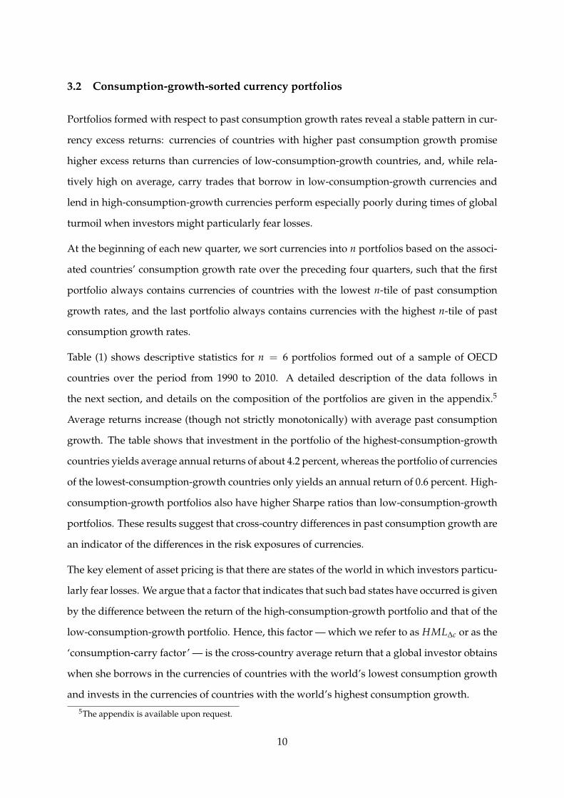
Portfolios formed with respect to past consumption growth rates reveal a stable pattern in cur-

rency excess returns: currencies of countries with higher past consumption growth promise

higher excess returns than currencies of low-consumption-growth countries, and, while rela-

tively high on average, carry trades that borrow in low-consumption-growth currencies and

lend in high-consumption-growth currencies perform especially poorly during times of global

turmoil when investors might particularly fear losses.

At the beginning of each new quarter, we sort currencies into n portfolios based on the associ-

ated countries’ consumption growth rate over the preceding four quarters, such that the first

portfolio always contains currencies of countries with the lowest n-tile of past consumption

growth rates, and the last portfolio always contains currencies with the highest n-tile of past

consumption growth rates.

Table (1) shows descriptive statistics for n = 6 portfolios formed out of a sample of OECD

countries over the period from 1990 to 2010. A detailed description of the data follows in

the next section, and details on the composition of the portfolios are given in the appendix.5

Average returns increase (though not strictly monotonically) with average past consumption

growth. The table shows that investment in the portfolio of the highest-consumption-growth

countries yields average annual returns of about 4.2 percent, whereas the portfolio of currencies

of the lowest-consumption-growth countries only yields an annual return of 0.6 percent. High-

consumption-growth portfolios also have higher Sharpe ratios than low-consumption-growth

portfolios. These results suggest that cross-country differences in past consumption growth are

an indicator of the differences in the risk exposures of currencies.

The key element of asset pricing is that there are states of the world in which investors particu-

larly fear losses. We argue that a factor that indicates that such bad states have occurred is given

by the difference between the return of the high-consumption-growth portfolio and that of the

low-consumption-growth portfolio. Hence, this factor — which we refer to as HML∆c or as the

‘consumption-carry factor’ — is the cross-country average return that a global investor obtains

when she borrows in the currencies of countries with the world’s lowest consumption growth

and invests in the currencies of countries with the world’s highest consumption growth.5The appendix is available upon request.

10

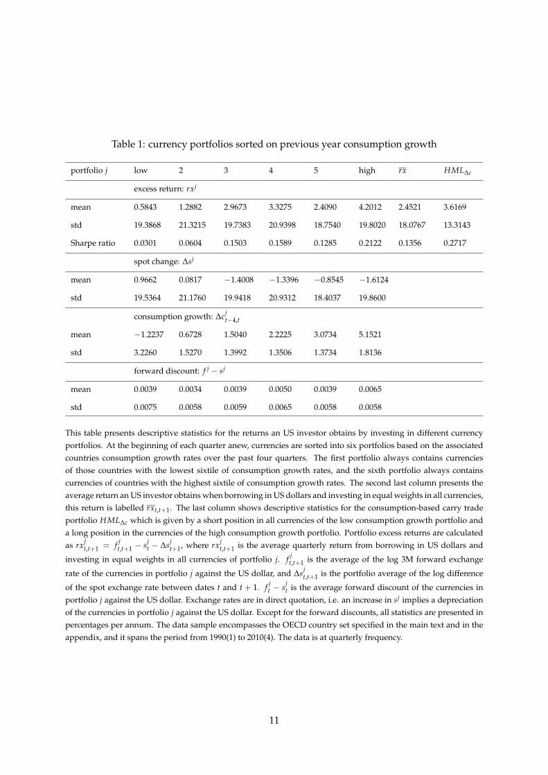
Table 1: currency portfolios sorted on previous year consumption growth

portfolio j low 2 3 4 5 high rx HML∆c

excess return: rxj

mean 0.5843 1.2882 2.9673 3.3275 2.4090 4.2012 2.4521 3.6169

std 19.3868 21.3215 19.7383 20.9398 18.7540 19.8020 18.0767 13.3143

Sharpe ratio 0.0301 0.0604 0.1503 0.1589 0.1285 0.2122 0.1356 0.2717

spot change: ∆sj

mean 0.9662 0.0817 −1.4008 −1.3396 −0.8545 −1.6124

std 19.5364 21.1760 19.9418 20.9312 18.4037 19.8600

consumption growth: ∆cjt−4,t

mean −1.2237 0.6728 1.5040 2.2225 3.0734 5.1521

std 3.2260 1.5270 1.3992 1.3506 1.3734 1.8136

forward discount: f j − sj

mean 0.0039 0.0034 0.0039 0.0050 0.0039 0.0065

std 0.0075 0.0058 0.0059 0.0065 0.0058 0.0058

This table presents descriptive statistics for the returns an US investor obtains by investing in different currencyportfolios. At the beginning of each quarter anew, currencies are sorted into six portfolios based on the associatedcountries consumption growth rates over the past four quarters. The first portfolio always contains currenciesof those countries with the lowest sixtile of consumption growth rates, and the sixth portfolio always containscurrencies of countries with the highest sixtile of consumption growth rates. The second last column presents theaverage return an US investor obtains when borrowing in US dollars and investing in equal weights in all currencies,this return is labelled rxt,t+1. The last column shows descriptive statistics for the consumption-based carry tradeportfolio HML∆c which is given by a short position in all currencies of the low consumption growth portfolio anda long position in the currencies of the high consumption growth portfolio. Portfolio excess returns are calculatedas rxj

t,t+1 = f jt,t+1 − sj

t − ∆sjt+1, where rxj

t,t+1 is the average quarterly return from borrowing in US dollars and

investing in equal weights in all currencies of portfolio j. f jt,t+1 is the average of the log 3M forward exchange

rate of the currencies in portfolio j against the US dollar, and ∆sjt,t+1 is the portfolio average of the log difference

of the spot exchange rate between dates t and t + 1. f jt − sj

t is the average forward discount of the currencies inportfolio j against the US dollar. Exchange rates are in direct quotation, i.e. an increase in sj implies a depreciationof the currencies in portfolio j against the US dollar. Except for the forward discounts, all statistics are presented inpercentages per annum. The data sample encompasses the OECD country set specified in the main text and in theappendix, and it spans the period from 1990(1) to 2010(4). The data is at quarterly frequency.

11

The last column of table (1) shows that this carry trade returns up to 3.6 percent a year, with

a Sharpe ratio of 0.27. The empirical analysis of the next section will reveal that this HML∆c

factor explains the cross-sectional difference in expected portfolio returns to a considerable

extent and that it is globally priced.

The second last column of table (1) shows descriptive statistics for rx, which is the average

return that an investor achieves by borrowing at the beginning of each quarter in US dollars

and investing in equal weights into all currencies available in the sample over a holding period

of one quarter. Lustig et al. (2011) call this factor the ‘dollar risk factor’, because it captures the

idiosyncratic (country-specific) component of an investment strategy that funds itself in dollars

and goes long in the cross section of all other currencies. At each point in time, the dollar

risk factor therefore essentially captures the average rate of depreciation of the dollar against

all other currencies. As this dollar factor is important for the level of all dollar-denominated

returns, it is important to include it in all our pricing exercises below. However, because of

its country-specific nature, we do not expect that this US dollar factor can explain the cross-

sectional difference in the returns of different currency portfolios. As argued by Lustig et al.

(2011), it should therefore not be globally priced. This means that there should be no differences

across currency portfolios in the exposure to this factor.

Conversely, we will show in the next sections that the HML∆c factor is globally priced — that

is, we will show that it prices the cross section of currencies exactly because currency portfolios

have different degrees of exposure to it.

A couple of remarks on the procedure for sorting currencies into portfolios based on past con-

sumption growth rates are in order. First, it is important to recognize that, over time, currencies

change portfolios, reflecting countries’ changing position in the cross-country distribution of

consumption growth rates. This is the essence of forming portfolios: the fact that individual

currencies may change portfolios reflects the fact that they may not have a fixed exposure to

the risk that we wish to price. This may imply that individual currencies do not have a constant

beta with respect to the risk factor HML∆C. However, as we will show, and as has also been

emphasized by Lustig and Verdelhan (2007) and Lustig et al. (2011), portfolios of currencies do

have a constant beta with respect to the risk factor HML∆C.6

6Note that the approach of building portfolios is also robust to missing data: for some countries, available

12

Second, we focus on consumption growth over the past four quarters to build currency port-

folios, instead of consumption growth rates at the highest available (i.e. quarterly) frequency.

This reflects the recent focus of the literature on the role of low- to medium-frequency compo-

nents in consumption for asset pricing. For example, quarterly consumption data might be a

very noisy measure of true consumption, so that averaging consumption growth over several

periods could provide a better approximation of the ultimate consumption risk that investors

care about.7 Alternatively, investors might have a preference for an early resolution of un-

certainty, so that small but potentially very persistent movements in long-term consumption

growth carry a much higher risk price than short-term fluctuations in consumption.8 Further-

more, forming portfolios over annual consumption growth rates is likely to make the formation

of consumption-based portfolios more easily implementable as a tradable strategy: consump-

tion data at a quarterly frequency may not be observable in real time because of publication

lags and frequent data revisions. Consumption growth at an annual frequency is plausibly

much less affected by this problem. Finally, building growth rates over one year implicitly also

deal with seasonal effects present in some of the consumption growth series.

3.3 The consumption carry factor HML∆c

This section discusses the consumption carry factor HML∆c in more detail and sets it in relation

to other pricing factors that have been proposed in the literature. Table (5) presents key statistics

for HML∆c, as well as for other factors: the mean return of the consumption-carry strategy is

3.6 percent per year, and the Sharpe ratio is around 0.27. These figures are both smaller than the

respective values for Lustig et al.’s (2011) forward-discount-based carry trade strategy HMLFX

consumption series do not span the whole sampling period, for other countries, forward exchange rates becameavailable only in the late 1990s, and euro countries are excluded from the sample after they introduced the commonEuropean currency.

7Within the framework of the basic consumption-based capital asset pricing model (C-CAPM), Jagannathan andWang (2007) show that the fourth quarter to fourth quarter consumption growth rate is a powerful pricing factor,and Parker and Julliard (2005) find that the covariance of returns and consumption growth across the 25 Famaand French (1989) portfolios explains the difference in expected returns observed in the US stock market extremelywell, if consumption growth is measured over the quarter of the return and many following quarters. Lettau andLudvigson (2001) reason that consumption should react predominantly to permanent shocks in wealth, such thatthe consumption-to-wealth ratio (cay) is unaffected. Fluctuations in cay therefore signal transitory variation inwealth (i.e. future returns), which implies that cay is a powerful pricing factor for asset returns.

8In the long-run risk models introduced by Bansal and Yaron (2004), consumption growth follows an ARMA(1,1)process with a slow-moving permanent component, such that shocks will affect consumption at a very long horizon.As agents dislike such long-run risk, a highly volatile consumption-based discount factor results, which has thepower to explain observed asset returns.

13

which, calculated using quarterly data, pays an average annual return of around 6.1 percent

with a Sharpe ratio of 0.30.

Figure 1: HMLFX against HML∆c

1992 1994 1996 1998 2000 2002 2004 2006 2008 2010

−0.15

−0.1

−0.05

0

0.05

0.1

HML ∆ c

HML FX

The blue solid line plots the consumption carry trade factor HML∆c, and the black, dotted line shows the Lustiget al. (2011) carry trade factor HMLFX . The HML∆c factor is the cross-country average return a global investorobtains when she borrows in the currencies of countries which experienced low consumption growth over the lastyear and invests in currencies of countries with high past consumption growth. The HMLFX factor corresponds tothe return obtained from borrowing in low interest rate currencies and lending in high interest rate currencies. Bothfactors have been constructed from quarterly data which encompass the OECD sample specified in the main text.

Figure (1) plots HML∆c against HMLFX. The correlation of the two factors is highly significant,

but at 0.36 far from perfect. Figure (1) suggests that HML∆c and HMLFX are particularly highly

correlated during some periods of global turmoil such as the Euro crisis of 1992, the Mexican

Peso crisis of 1994, September 11 2001 and the Bear Stearns bankruptcy in August 2007. The

returns also often comove during more tranquil periods. Interestingly, the two factors do not

strongly move together during the Lehman shock in 2008, whereby the consumption-based

carry trade strategy provided distinctly less volatile returns than the forward-discount-based

carry trade strategy. In fact, the returns from the consumption- based carry trade strategy are

substantially less skewed than HMLFX (with a standardized third moment of 0.08 for HML∆c

as opposed to −0.84 for HMLFX). With regard to its relation to traditional pricing factors

14

motivated by the (C-)CAPM, consumption carry trade returns are basically uncorrelated with

world average consumption growth and with the global stock market return as measured by

the MSCI world index. However, HML∆c is significantly negatively correlated with the cross-

country variance of consumption growth rates. After examining the data set in the next section,

Section (5) will reveal that the consumption- based carry trade factor HML∆c indeed mirrors

risk that is priced in currency markets.

4 The data

The main data set used in this analysis includes time series of quarterly consumption growth

rates, as well as daily midpoint quotes of spot and forward exchange rates for a cross section of

33 OECD countries, which are Australia, Austria, Belgium, Canada, Chile, the Czech Republic,

Denmark, Estonia, Finland, France, Germany, Greece, Hungary, Ireland, Iceland, Israel, Italy,

Japan, South Korea, Mexico, Netherlands, New Zealand, Norway, Poland, Portugal, the Slovak

Republic, Slovenia, Spain, Sweden, Switzerland, the United Kingdom, the United States and

the euro area. Quarterly spot and forward exchange rate series are the quoted price of the last

trading day of each quarter. Consumption growth rates are measured in real per capita terms,

and quarterly population estimates are obtained by linearly interpolating annual population

figures. The main analysis uses a data set that spans the period from the first quarter of 1990

to the fourth quarter of 2010; in the appendix, we also present results obtained from using

a longer data set that starts in the first quarter of 1986. The data are sourced from various

providers accessed via Datastream and from OECD.Stat9, and consumption price index series

are sourced from the IFS. Details on the source and time span of the data for each country are

listed in Table (11) in the appendix.

9OECD (2012), OECD.Stat, (database). http://stats.oecd.org/Index.aspx (Accessed on 02 August 2012)

15

5 Empirical results

5.1 Pricing currency returns

The price of an asset equals its expected discounted payoff. This price reflects the nondiversifi-

able component of risk associated with a particular asset, which is determined by its exposure

to a set of common risk factors. As carry trades are a zero-net-investment strategy, if the law of

one price holds, the return on each portfolio j, denoted by rxjt+1, must satisfy

0 = E(Mt,t+1rxjt,t+1) (4)

where Mt+1 denotes the stochastic discount factor that prices the payoffs denominated in US

dollars. We assume that the stochastic discount factor M is linear in the pricing factors

Mt+1 = 1− b′ f ′t+1 (5)

where f t+1 denotes a matrix of risk factors containing the different factors in its columns, and

b is the column vector of factor loadings. Equation (4) and (5) imply that

E(rxjt+1) = −

(cov(Mt+1, rxj

t+1)var(Mt+1)−1) (

var(Mt+11)E(Mt+1)−1)

= βj′λ (6)

where the column vectors βj contain regression coefficients that are obtained by running time

series regressions of portfolio returns rxj on the factors of the stochastic discount factor. The

market price of risk λ mirrored by each factor can be estimated by running a cross-sectional

regression of expected portfolio returns on βj. Substituting the expression for the stochastic

discount factor (5) into the Euler equation (4) yields the following alternative expression for

the expected returns of currency portfolio j

E(rxjt+1) = cov( f t+1, rxj

t+1)′b (7)

16

where cov(.) denotes the vector of covariances of the individual elements of f with rx. Hence,

the market price of risk λ and the factor loadings b are related by λ = var( f t+1)b where

var(.) denotes the covariance matrix of the individual elements of f . The factor loadings b are

estimated by a cross-sectional regression of expected excess returns on the covariance between

returns and factors.

Our specification for the stochastic discount factor includes two factors

Mt+1 = 1− brx · rxt+1 − bHML ∆c · HML ∆ct+1

where our main interest is on the consumption carry trade factor HML∆c. As we will argue,

HML∆c acts as a global slope factor that determines return differences in the cross section of

currency excess returns. As a second factor, we include the return to a US investor who owns an

equal-weighted portfolio of the cross section of all currencies. As shown by Lustig et al. (2011),

this factor, referred to as rx, captures base-currency-specific (here: dollar-specific) influences on

the cross section of currency returns. It is therefore an idiosyncratic factor and acts as a level

shifter for all dollar-denominated returns.

Time series regression

A factor mirrors global risk if differences in expected returns across portfolios can be explained

by differences in the extent to which portfolios load on this factor. We obtain the loadings or

βs on the risk factors rx and HML∆c by running the following time series regression separately

for each currency portfolio j.

rxjt,t+1 = aj + β

jrx · rxt,t+1 + β

jHML ∆c · HML ∆ct,t+1 + ε

jt,t+1 (8)

Figure (2) plots the estimate of βjHML ∆c for each currency portfolio j against its mean excess

return. The low-consumption-growth portfolio pays the lowest returns on average, and its

correlation with HML∆c is relatively low: in bad times, when HML∆c declines, this portfolio

still performs relatively well and thus shields an investor’s income stream against low returns.

In contrast, the return of the high-consumption- growth portfolio covaries more strongly with

HML∆c. Indeed, the estimates of βjHML ∆c increase almost monotonically from low- to high-

17

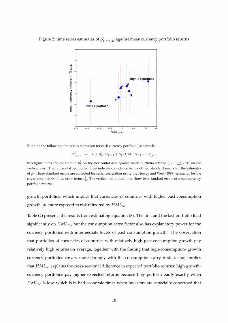
Figure 2: time series estimates of βjHML dc against mean currency portfolio returns

−0.8 −0.6 −0.4 −0.2 0 0.2 0.4 0.6−4

−2

0

2

4

6

8

10

mean c

urr

ency r

etu

rns in %

p.a

.

βHML_∆ c

low ∆ c portfolio

2

34

5

high ∆ c portfolio

Running the following time series regression for each currency portfolio j separately,

rxjt,t+1 = αj + β

j1 · rxt,t+1 + β

j2 · HML ∆ct,t+1 + ε

jt,t+1

this figure plots the estimate of βj2 on the horizontal axis against mean portfolio returns (1/T)∑T

t=1 rxjt on the

vertical axis. The horizontal red dotted lines indicate confidence bands of two standard errors for the estimatesof β2 These standard errors are corrected for serial correlation using the Newey and West (1987) estimator for thecovariance matrix of the error terms ε

jt,. The vertical red dotted lines show two standard errors of mean currency

portfolio returns.

growth portfolios, which implies that currencies of countries with higher past consumption

growth are more exposed to risk mirrored by HML∆c.

Table (2) presents the results from estimating equation (8). The first and the last portfolio load

significantly on HML∆c, but the consumption carry factor also has explanatory power for the

currency portfolios with intermediate levels of past consumption growth. The observation

that portfolios of currencies of countries with relatively high past consumption growth pay

relatively high returns on average, together with the finding that high-consumption- growth

currency portfolios covary more strongly with the consumption carry trade factor, implies

that HML∆c explains the cross-sectional difference in expected portfolio returns: high-growth-

currency portfolios pay higher expected returns because they perform badly exactly when

HML∆c is low, which is in bad economic times when investors are especially concerned that

18

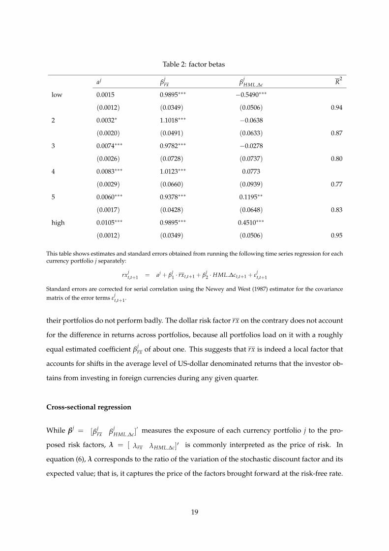
Table 2: factor betas

aj βjrx β

jHML ∆c R2

low 0.0015 0.9895∗∗∗ −0.5490∗∗∗

(0.0012) (0.0349) (0.0506) 0.94

2 0.0032∗ 1.1018∗∗∗ −0.0638

(0.0020) (0.0491) (0.0633) 0.87

3 0.0074∗∗∗ 0.9782∗∗∗ −0.0278

(0.0026) (0.0728) (0.0737) 0.80

4 0.0083∗∗∗ 1.0123∗∗∗ 0.0773

(0.0029) (0.0660) (0.0939) 0.77

5 0.0060∗∗∗ 0.9378∗∗∗ 0.1195∗∗

(0.0017) (0.0428) (0.0648) 0.83

high 0.0105∗∗∗ 0.9895∗∗∗ 0.4510∗∗∗

(0.0012) (0.0349) (0.0506) 0.95

This table shows estimates and standard errors obtained from running the following time series regression for eachcurrency portfolio j separately:

rxjt,t+1 = aj + β

j1 · rxt,t+1 + β

j2 · HML ∆ct,t+1 + ε

jt,t+1

Standard errors are corrected for serial correlation using the Newey and West (1987) estimator for the covariancematrix of the error terms ε

jt,t+1.

their portfolios do not perform badly. The dollar risk factor rx on the contrary does not account

for the difference in returns across portfolios, because all portfolios load on it with a roughly

equal estimated coefficient βjrx of about one. This suggests that rx is indeed a local factor that

accounts for shifts in the average level of US-dollar denominated returns that the investor ob-

tains from investing in foreign currencies during any given quarter.

Cross-sectional regression

While βj = [βjrx β

jHML ∆c]

′ measures the exposure of each currency portfolio j to the pro-

posed risk factors, λ = [ λrx λHML ∆c]′ is commonly interpreted as the price of risk. In

equation (6), λ corresponds to the ratio of the variation of the stochastic discount factor and its

expected value; that is, it captures the price of the factors brought forward at the risk-free rate.

19

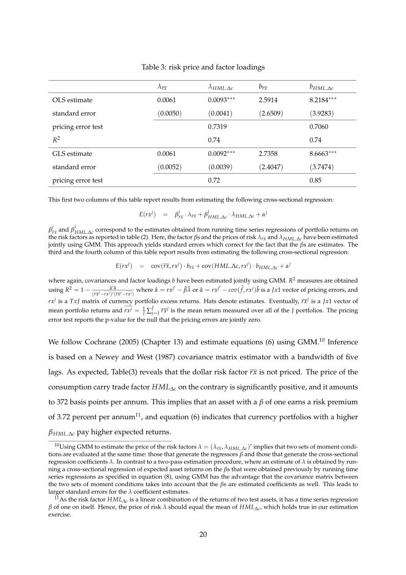
Table 3: risk price and factor loadings

λrx λHML ∆c brx bHML ∆c

OLS estimate 0.0061 0.0093∗∗∗ 2.5914 8.2184∗∗∗

standard error (0.0050) (0.0041) (2.6509) (3.9283)

pricing error test 0.7319 0.7060

R2 0.74 0.74

GLS estimate 0.0061 0.0092∗∗∗ 2.7358 8.6663∗∗∗

standard error (0.0052) (0.0039) (2.4047) (3.7474)

pricing error test 0.72 0.85

This first two columns of this table report results from estimating the following cross-sectional regression:

E(rxj) = βjrx · λrx + β

jHML ∆c · λHML ∆c + αj

βjrx and β

jHML ∆c correspond to the estimates obtained from running time series regressions of portfolio returns on

the risk factors as reported in table (2). Here, the factor βs and the prices of risk λrx and λHML ∆c have been estimatedjointly using GMM. This approach yields standard errors which correct for the fact that the βs are estimates. Thethird and the fourth column of this table report results from estimating the following cross-sectional regression:

E(rxj) = cov(rx, rxj) · brx + cov(HML ∆c, rxj) · bHML ∆c + αj

where again, covariances and factor loadings b have been estimated jointly using GMM. R2 measures are obtainedusing R2 = 1− α′ α

(rxj−rxj)′(rxj−rxj)where α = rxj′ − βλ or α = rxj′ − ˆcov( f , rxj)b is a Jx1 vector of pricing errors, and

rxj is a TxJ matrix of currency portfolio excess returns. Hats denote estimates. Eventually, rxj is a Jx1 vector ofmean portfolio returns and rxj = 1

J ∑Jj=1 rxj is the mean return measured over all of the J portfolios. The pricing

error test reports the p-value for the null that the pricing errors are jointly zero.

We follow Cochrane (2005) (Chapter 13) and estimate equations (6) using GMM.10 Inference

is based on a Newey and West (1987) covariance matrix estimator with a bandwidth of five

lags. As expected, Table(3) reveals that the dollar risk factor rx is not priced. The price of the

consumption carry trade factor HML∆c on the contrary is significantly positive, and it amounts

to 372 basis points per annum. This implies that an asset with a β of one earns a risk premium

of 3.72 percent per annum11, and equation (6) indicates that currency portfolios with a higher

βHML ∆c pay higher expected returns.

10Using GMM to estimate the price of the risk factors λ = (λrx, λHML ∆c)′ implies that two sets of moment condi-

tions are evaluated at the same time: those that generate the regressors β and those that generate the cross-sectionalregression coefficients λ. In contrast to a two-pass estimation procedure, where an estimate of λ is obtained by run-ning a cross-sectional regression of expected asset returns on the βs that were obtained previously by running timeseries regressions as specified in equation (8), using GMM has the advantage that the covariance matrix betweenthe two sets of moment conditions takes into account that the βs are estimated coefficients as well. This leads tolarger standard errors for the λ coefficient estimates.

11As the risk factor HML∆c is a linear combination of the returns of two test assets, it has a time series regressionβ of one on itself. Hence, the price of risk λ should equal the mean of HML∆c, which holds true in our estimationexercise.

20

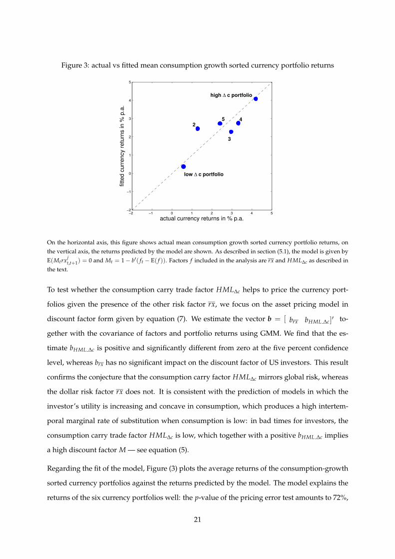
Figure 3: actual vs fitted mean consumption growth sorted currency portfolio returns

−2 −1 0 1 2 3 4 5−2

−1

0

1

2

3

4

5

actual currency returns in % p.a.

fitted c

urr

ency r

etu

rns in %

p.a

.

low ∆ c portfolio

2

3

45

high ∆ c portfolio

On the horizontal axis, this figure shows actual mean consumption growth sorted currency portfolio returns, onthe vertical axis, the returns predicted by the model are shown. As described in section (5.1), the model is given byE(Mtrxj

t,t+1) = 0 and Mt = 1− b′( ft − E( f )). Factors f included in the analysis are rx and HML∆c as described inthe text.

To test whether the consumption carry trade factor HML∆c helps to price the currency port-

folios given the presence of the other risk factor rx, we focus on the asset pricing model in

discount factor form given by equation (7). We estimate the vector b = [ brx bHML ∆c]′ to-

gether with the covariance of factors and portfolio returns using GMM. We find that the es-

timate bHML ∆c is positive and significantly different from zero at the five percent confidence

level, whereas brx has no significant impact on the discount factor of US investors. This result

confirms the conjecture that the consumption carry factor HML∆c mirrors global risk, whereas

the dollar risk factor rx does not. It is consistent with the prediction of models in which the

investor’s utility is increasing and concave in consumption, which produces a high intertem-

poral marginal rate of substitution when consumption is low: in bad times for investors, the

consumption carry trade factor HML∆c is low, which together with a positive bHML ∆c implies

a high discount factor M — see equation (5).

Regarding the fit of the model, Figure (3) plots the average returns of the consumption-growth

sorted currency portfolios against the returns predicted by the model. The model explains the

returns of the six currency portfolios well: the p-value of the pricing error test amounts to 72%,

21

which implies that we cannot reject the null that the pricing errors from the cross-sectional

regression of mean currency portfolio returns on the βs equal zero.

These results suggest that HML∆c captures global risk in the world cross section of currencies.

In the next section, we examine whether HML∆c prices a cross section of test portfolios that

have been sorted by forward discounts (as in Lustig et al. (2011)) and compare the pricing

power of the consumption carry factor to that of two other extant factors, the Lustig et al.

(2011) HMLFX factor and the Menkhoff et al. (2012) foreign exchange volatility innovation

factor, which have both been constructed from purely financial information.

5.2 Forward-discount-sorted currency portfolios and further risk factors

If the consumption carry trade factor HML∆c mirrors global, nondiversifiable risk, this factor

should explain the difference in expected returns of any assets. Initiated by Lustig and Verdel-

han (2007), the most commonly used test assets in the current literature on currency pricing are

forward-discount-sorted currency portfolios. The results presented in Table (4) suggest that

the consumption carry trade factor prices this cross section of test assets as well, and that it

compares favorably to other risk factors proposed by the literature.

In Table (4), the test assets are six currency portfolios that have been constructed for each quar-

ter by sorting the currencies of the OECD data sample on their forward discount toward the US

observed at the end of the preceding quarter. Descriptive statistics for these forward-discount-

sorted currency portfolios are provided in Table (B.6) in the Appendix. Using this set of test

assets, we estimate the price of the consumption carry trade factor HML∆c to be 908 basis points

a year, and it is significantly different from zero at the five percent confidence level.

The second and third columns of Table (4) show estimates of risk prices and factor loadings for

two further risk factors; namely, for the Lustig et al. (2011) HMLFX factor and the Menkhoff

et al. (2012) foreign exchange volatility innovation VOL factor. We have constructed both risk

factors as described in the respective papers using the quarterly data of the OECD sample

specified in Section (4). Both risk factors, HMLFX and VOL, are able to price the quarterly

forward-discount-sorted currency portfolios.

22

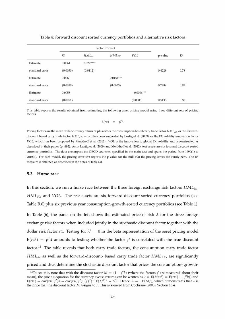
Table 4: forward discount sorted currency portfolios and alternative risk factors

Factor Prices λ

rx HML∆c HMLFX VOL p-value R2

Estimate 0.0061 0.0227∗∗∗

standard error (0.0050) (0.0112) 0.4229 0.78

Estimate 0.0060 0.0154∗∗∗

standard error (0.0050) (0.0053) 0.7489 0.87

Estimate 0.0058 −0.0006∗∗∗

standard error (0.0051) (0.0003) 0.5133 0.80

This table reports the results obtained from estimating the following asset pricing model using three different sets of pricingfactors

E(rx) = β′λ

Pricing factors are the mean dollar currency return rx plus either the consumption-based carry trade factor HML∆c, or the forward-

discount based carry trade factor HMLFX , which has been suggested by Lustig et al. (2009), or the FX volatiliy innovation factor

VOL, which has been proposed by Menkhoff et al. (2012). VOL is the innovation to global FX volatiliy and is constructed as

described in their paper (p. 692). As in Lustig et al. (2009) and Menkhoff et al. (2012), test assets are six forward discount sorted

currency portfolios. The data encompass the OECD countries specified in the main text and spans the period from 1990(1) to

2010(4). For each model, the pricing error test reports the p-value for the null that the pricing errors are jointly zero. The R2

measure is obtained as described in the notes of table (3).

5.3 Horse race

In this section, we run a horse race between the three foreign exchange risk factors HML∆c,

HMLFX and VOL. The test assets are six forward-discount-sorted currency portfolios (see

Table B.6) plus six previous year consumption-growth-sorted currency portfolios (see Table 1).

In Table (6), the panel on the left shows the estimated price of risk λ for the three foreign

exchange risk factors when included jointly in the stochastic discount factor together with the

dollar risk factor rx. Testing for λi = 0 in the beta representation of the asset pricing model

E(rxj) = βjλ amounts to testing whether the factor f i is correlated with the true discount

factor.12 The table reveals that both carry trade factors, the consumption carry trade factor

HML∆c as well as the forward-discount- based carry trade factor HMLFX, are significantly

priced and thus determine the stochastic discount factor that prices the consumption- growth-

12To see this, note that with the discount factor M = (1− f ′b) (where the factors f are measured about theirmean), the pricing equation for the currency excess returns can be written as 0 = E(Mrxj) = E(rxj(1− f ′b)) andE(rxj) = cov(rxj, f ′)b = cov(rxj, f ′)E( f f ′)−1E( f f ′)b = β′λ. Hence, λ = −E(M f ), which demonstrates that λ isthe price that the discount factor M assigns to f . This is sourced from Cochrane (2005), Section 13.4.

23

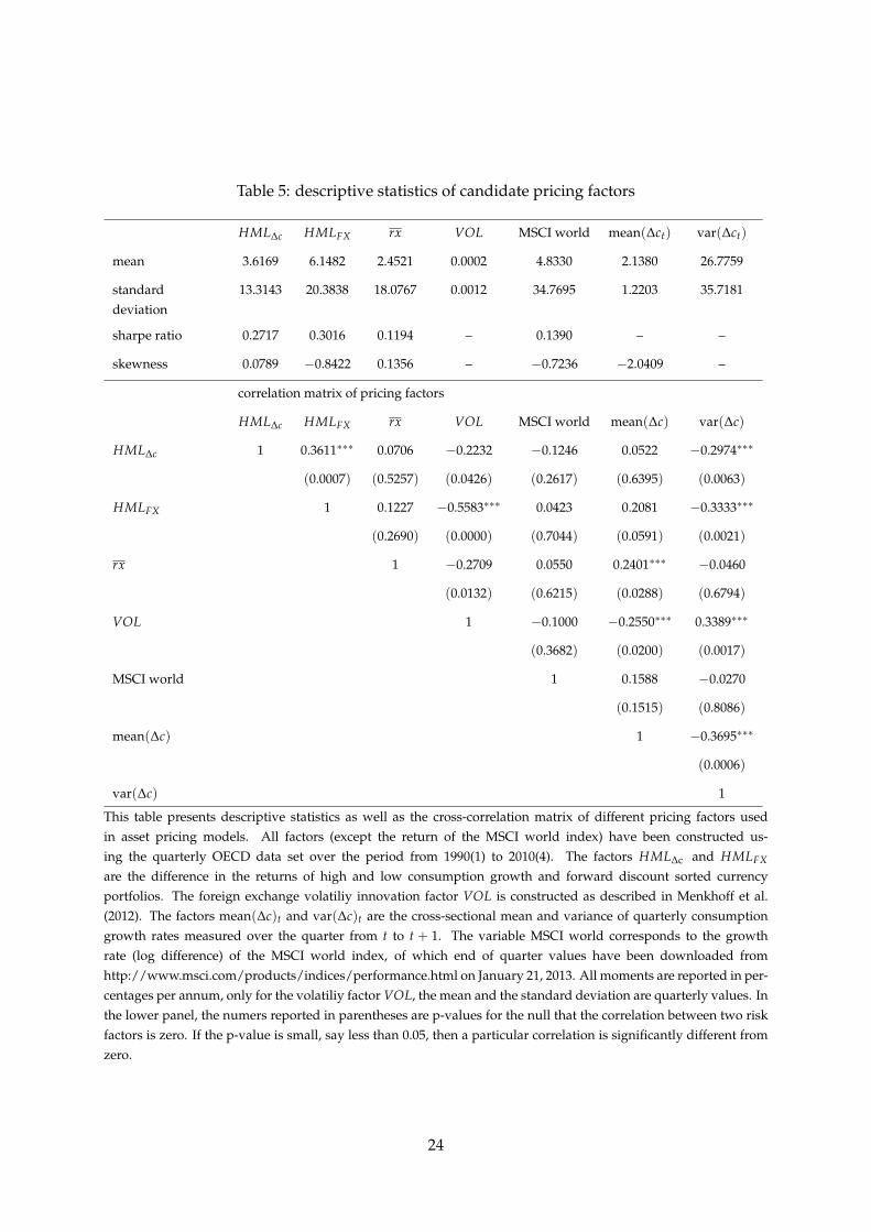
Table 5: descriptive statistics of candidate pricing factors

HML∆c HMLFX rx VOL MSCI world mean(∆ct) var(∆ct)

mean 3.6169 6.1482 2.4521 0.0002 4.8330 2.1380 26.7759

standarddeviation

13.3143 20.3838 18.0767 0.0012 34.7695 1.2203 35.7181

sharpe ratio 0.2717 0.3016 0.1194 – 0.1390 – –

skewness 0.0789 −0.8422 0.1356 – −0.7236 −2.0409 –

correlation matrix of pricing factors

HML∆c HMLFX rx VOL MSCI world mean(∆c) var(∆c)

HML∆c 1 0.3611∗∗∗ 0.0706 −0.2232 −0.1246 0.0522 −0.2974∗∗∗

(0.0007) (0.5257) (0.0426) (0.2617) (0.6395) (0.0063)

HMLFX 1 0.1227 −0.5583∗∗∗ 0.0423 0.2081 −0.3333∗∗∗

(0.2690) (0.0000) (0.7044) (0.0591) (0.0021)

rx 1 −0.2709 0.0550 0.2401∗∗∗ −0.0460

(0.0132) (0.6215) (0.0288) (0.6794)

VOL 1 −0.1000 −0.2550∗∗∗ 0.3389∗∗∗

(0.3682) (0.0200) (0.0017)

MSCI world 1 0.1588 −0.0270

(0.1515) (0.8086)

mean(∆c) 1 −0.3695∗∗∗

(0.0006)

var(∆c) 1

This table presents descriptive statistics as well as the cross-correlation matrix of different pricing factors usedin asset pricing models. All factors (except the return of the MSCI world index) have been constructed us-ing the quarterly OECD data set over the period from 1990(1) to 2010(4). The factors HML∆c and HMLFX

are the difference in the returns of high and low consumption growth and forward discount sorted currencyportfolios. The foreign exchange volatiliy innovation factor VOL is constructed as described in Menkhoff et al.(2012). The factors mean(∆c)t and var(∆c)t are the cross-sectional mean and variance of quarterly consumptiongrowth rates measured over the quarter from t to t + 1. The variable MSCI world corresponds to the growthrate (log difference) of the MSCI world index, of which end of quarter values have been downloaded fromhttp://www.msci.com/products/indices/performance.html on January 21, 2013. All moments are reported in per-centages per annum, only for the volatiliy factor VOL, the mean and the standard deviation are quarterly values. Inthe lower panel, the numers reported in parentheses are p-values for the null that the correlation between two riskfactors is zero. If the p-value is small, say less than 0.05, then a particular correlation is significantly different fromzero.

24

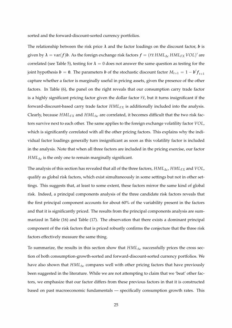
sorted and the forward-discount-sorted currency portfolios.

The relationship between the risk price λ and the factor loadings on the discount factor, b is

given by λ = var( f )b. As the foreign exchange risk factors f = (rx HML∆c HMLFX VOL)′ are

correlated (see Table 5), testing for λ = 0 does not answer the same question as testing for the

joint hypothesis b = 0. The parameters b of the stochastic discount factor Mt+1 = 1− b′ f t+1

capture whether a factor is marginally useful in pricing assets, given the presence of the other

factors. In Table (6), the panel on the right reveals that our consumption carry trade factor

is a highly significant pricing factor given the dollar factor rx, but it turns insignificant if the

forward-discount-based carry trade factor HMLFX is additionally included into the analysis.

Clearly, because HMLFX and HML∆c are correlated, it becomes difficult that the two risk fac-

tors survive next to each other. The same applies to the foreign exchange volatility factor VOL,

which is significantly correlated with all the other pricing factors. This explains why the indi-

vidual factor loadings generally turn insignificant as soon as this volatility factor is included

in the analysis. Note that when all three factors are included in the pricing exercise, our factor

HML∆c is the only one to remain marginally significant.

The analysis of this section has revealed that all of the three factors, HML∆c, HMLFX and VOL,

qualify as global risk factors, which exist simultaneously in some settings but not in other set-

tings. This suggests that, at least to some extent, these factors mirror the same kind of global

risk. Indeed, a principal components analysis of the three candidate risk factors reveals that

the first principal component accounts for about 60% of the variability present in the factors

and that it is significantly priced. The results from the principal components analysis are sum-

marized in Table (16) and Table (17). The observation that there exists a dominant principal

component of the risk factors that is priced robustly confirms the conjecture that the three risk

factors effectively measure the same thing.

To summarize, the results in this section show that HML∆c successfully prices the cross sec-

tion of both consumption-growth-sorted and forward-discount-sorted currency portfolios. We

have also shown that HML∆c compares well with other pricing factors that have previously

been suggested in the literature. While we are not attempting to claim that we ‘beat’ other fac-

tors, we emphasize that our factor differs from these previous factors in that it is constructed

based on past macroeconomic fundamentals — specifically consumption growth rates. This

25

suggests that international differences in medium-term consumption growth are informative

with respect to the risk exposure of a country’s currency to global shocks.

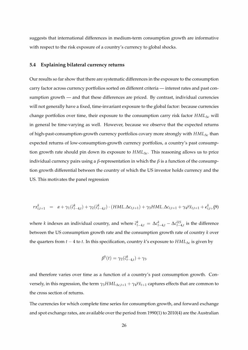
5.4 Explaining bilateral currency returns

Our results so far show that there are systematic differences in the exposure to the consumption

carry factor across currency portfolios sorted on different criteria — interest rates and past con-

sumption growth — and that these differences are priced. By contrast, individual currencies

will not generally have a fixed, time-invariant exposure to the global factor: because currencies

change portfolios over time, their exposure to the consumption carry risk factor HML∆c will

in general be time-varying as well. However, because we observe that the expected returns

of high-past-consumption-growth currency portfolios covary more strongly with HML∆c than

expected returns of low-consumption-growth currency portfolios, a country’s past consump-

tion growth rate should pin down its exposure to HML∆c. This reasoning allows us to price

individual currency pairs using a β-representation in which the β is a function of the consump-

tion growth differential between the country of which the US investor holds currency and the

US. This motivates the panel regression

rxkt,t+1 = a + γ1(ck

t−4,t) + γ2(ckt−4,t) · (HML ∆ct,t+1) + γ3HML ∆ct,t+1 + γ4rxt,t+1 + εk

t,t+1(9)

where k indexes an individual country, and where ckt−4,t = ∆ck

t−4,t − ∆cUSt−4,t is the difference

between the US consumption growth rate and the consumption growth rate of country k over

the quarters from t− 4 to t. In this specification, country k’s exposure to HML∆c is given by

βk(t) = γ2(ckt−4,t) + γ3

and therefore varies over time as a function of a country’s past consumption growth. Con-

versely, in this regression, the term γ3HML∆c,t+1 + γ4rxt+1 captures effects that are common to

the cross section of returns.

The currencies for which complete time series for consumption growth, and forward exchange

and spot exchange rates, are available over the period from 1990(1) to 2010(4) are the Australian

26

Tabl

e6:

hors

era

ce

risk

pric

eλ

fact

orlo

adin

gsb

rxH

ML ∆

cH

ML F

XV

OL

p-va

lue

rxH

ML ∆

cH

ML F

XV

OL

p-va

lue

R2

Esti

mat

e0.

0061

0.01

30∗∗∗

2.41

3111

.636∗∗∗

stan

dard

erro

r(0

.005

0)(0

.005

1)0.

4227

(2.7

888)

(4.6

745)

0.31

430.

63

Esti

mat

e0.

0061

0.01

65∗∗∗

2.15

906.

1881∗∗

stan

dard

erro

r(0

.005

0)(0

.005

5)0.

6487

(3.1

050)

(3.2

900)

0.63

160.

77

Esti

mat

e0.

0060

−0.

0007∗∗∗

−0.

2164

−42

7.49∗

stan

dard

erro

r(0

.005

0)(0

.000

3)0.

5344

(3.4

709)

(312

.13)

0.45

080.

73

Esti

mat

e0.

0061

0.00

89∗∗

0.01

52∗∗∗

2.11

805.

4605

4.42

13∗

stan

dard

erro

r(0

.005

0)(0

.004

6)(0

.005

4)0.

8576

(3.0

035)

(4.6

274)

(3.1

869)

0.81

210.

84

Esti

mat

e0.

0061

0.01

65∗∗∗

−0.

0002

2.33

036.

6029

30.2

5

stan

dard

erro

r(0

.005

0)(0

.005

3)(0

.000

5)0.

6103

(4.3

413)

(6.8

997)

(531

.01)

0.60

710.

77

Esti

mat

e0.

0060

0.00

88∗∗∗

−0.

0005∗∗

0.51

665.

6008

−29

1.85

stan

dard

erro

r(0

.005

0)(0

.004

2)(0

.000

3)0.

5232

(3.0

842)

(4.8

028)

(279

.70)

0.40

340.

80

Esti

mat

e0.

0061

0.00

94∗∗∗

0.01

55∗∗∗

0.00

003.

5480

6.16

65∗

7.66

7725

3.41

stan

dard

erro

r(0

.005

0)(0

.004

1)(0

.005

3)(0

.000

5)0.

8824

(4.3

158)

(4.2

124)

(6.4

531)

(461

.98)

0.85

680.

85

The

pane

lon

the

left

repo

rts

OLS

cros

s-se

ctio

nalr

egre

ssio

nes

tim

atio

nre

sult

sfo

rth

efo

llow

ing

mod

el:E

(rx)

=β′ λ

,

and

the

pane

lon

the

righ

trep

orts

OLS

cros

s-se

ctio

nalr

egre

ssio

nes

tim

atio

nre

sult

sfo

rth

efo

llow

ing

mod

el:E

(rx)

=co

v(f,

rx)′

b.

The

fact

orβ

san

dth

epr

ice

ofri

skλ

,as

wel

las

fact

orlo

adin

gsb

and

the

cova

rian

ces

betw

een

fact

ors

fan

dte

stas

setr

etur

nsrx

have

been

esti

mat

edjo

intl

yus

ing

GM

M(f

orde

tails

see

Coc

hran

e,20

05,

chap

ter

13).

Test

asse

tsar

esi

xco

nsum

pito

n-gr

owth

sort

edcu

rren

cypo

rtfo

lios

whi

char

eco

nstr

ucte

das

desc

ribe

din

the

mai

nte

xtpl

ussi

xfo

rwar

ddi

scou

ntso

rted

curr

ency

port

folio

s.A

sin

Lust

ig

etal

.(20

09),

forw

ard

disc

ount

sort

edpo

rtfo

lios

are

obta

ined

byso

rtin

gcu

rren

cies

into

port

folio

sac

cord

ing

toth

eir

prev

ious

end

ofqu

arte

rfo

rwar

ddi

scou

ntto

war

dsth

eU

Sdo

llar.

Pric

ing

fact

ors

are

the

mea

ndo

llar

curr

ency

retu

rnrx

and

HM

L ∆c

whi

char

ede

scri

bed

inth

em

ain

text

.H

ML ∆

cis

base

don

six

cons

umpt

ion-

grow

thso

rted

curr

ency

port

folio

s.T

heH

ML F

Xfa

ctor

corr

espo

nds

toth

e

pric

ing

fact

orsu

gges

ted

byLu

stig

etal

.(20

09,2

011)

.Iti

sth

ere

turn

ofa

carr

ytr

ade

stra

tegy

that

borr

ows

atth

ebe

ginn

ing

ofea

chqu

arte

rin

low

inte

rest

rate

curr

enci

esan

din

vest

sin

high

inte

rest

rate

curr

enci

es.

The

four

thpr

icin

gfa

ctor

,VO

L,ha

sbe

ensu

gges

ted

byM

enkh

off

etal

.(20

12).

Itis

the

inno

vati

onto

glob

alFX

vola

tiliy

and

isco

nstr

ucte

das

desc

ribe

din

thei

rpa

per

(p.

692)

.A

llpr

icin

g

fact

ors

asw

ella

sth

ete

stas

sets

are

obta

ined

from

the

OEC

Dda

tase

tspe

cifie

din

the

mai

nte

xtan

dth

eysp

anth

epe

riod

from

1990

(1)t

o20

10(4

).Fo

rea

chm

odel

,the

pric

ing

erro

rte

stre

port

sth

ep-

valu

e

for

the

null

that

the

pric

ing

erro

rsar

ejo

intl

yze

ro.T

head

just

edR

2ar

eob

tain

edas

desc

ribe

din

the

note

sof

tabl

e(3

).

27

dollar, the Canadian dollar, the Danish krone, the Japanese yen, the New Zealand dollar, the

Norwegian krone, the Swedish krona, the Swiss franc and the British pound. Table (7) shows

the results from the bilateral pricing regression (9) based on these nine currencies.

Note first that the interaction of HML∆c with past country-level consumption growth — the

coefficient γ2 — is positive and significant, whereas γ3 is not significant. This underpins the

interpretation of HML∆c as a global slope factor that explains differences in returns between

currencies provided that these countries have different consumption growth rates. As countries

change their position in the cross-sectional distribution of past consumption growth rates, their

exposure to HML∆c will change as well. Conversely, HML∆c does not impact the average

dollar-denominated return on foreign currency. This role of a level factor is, again, mainly

played by rx, which loads with a coefficient of virtually one on the cross section of currency

returns.

To illustrate further that differences in the exposure to HML∆c explain the cross section of

currency returns and that rx fully captures level shifts in dollar-denominated returns, we also

estimate a version of the panel regression in which we control for time- and country-fixed

effects

rxkt,t+1 = γ1(ck

t−4,t) + γ2(ckt−4,t) · (HML ∆ct,t+1) + τt + δk + εk

t,t+1 (10)

where the terms δk and τt denote country- and time-fixed effects. This panel regression displays

a very similar level of fit to the pricing regression above, and the coefficients γ1 and γ2 are also

very similar and significant; see Table (7). This illustrates that potentially unobserved country

characteristics do not affect the results regarding the sensitivity of individual currencies with

respect to the common risk factor HML∆c. It is also interesting to note that the estimate of the

time-fixed effect τt in equation (10) is closely linked to the dollar risk factor rxt: the correlation

of the two series is about 0.96. This confirms that the dollar risk factor — the average return

an investor gains by borrowing in US dollars and investing in all currencies available in the

market — provides a level factor for the cross section of dollar returns.

Regressions (9) and (10) suggest that excess returns from currency investment are related to

past consumption growth even at the level of individual currencies: because both γ1 and γ2 are

28

Table 7: pricing the cross-section of individual currencies: panel estimation

γ1 γ2 γ3 γ4 τt δk R2

rxkt,t+1 = a + γ1

(∆ck

t−4,t − ∆cUSt−4,t

)+ γ2

(∆ck

t−4,t − ∆cUSt−4,t

)· (HML∆c)t,t+1 + γ3 (HML∆c)t,t+1 + γ4rxt,t+1 + εt,t+1

estimate 0.1664∗∗∗ 8.2512∗∗∗ −0.0401 0.8979∗∗∗

se (0.0652) (2.3891) (0.0541) (0.0552) 0.53

rxkt,t+1 = γ1

(∆ck

t−4,t − ∆cUSt−4,t

)+ γ2

(∆ck

t−4,t − ∆cUSt−4,t

)· (HML∆c)t,t+1 + τt.t+1 + δk + εt,t+1

estimate 0.1257∗ 13.3064∗∗∗ yes yes

se (0.0802) (3.0713) 0.51

−∆skt,t+1 = a + γ1

(∆ck

t−4,t − ∆cUSt−4,t

)+ γ2

(∆ck

t−4,t − ∆cUSt−4,t

)· (HML∆c)t,t+1 + γ3 (HML∆c)t,t+1 + γ4rxt,t+1 + εt,t+1

estimate 0.1299∗∗ 8.5076∗∗∗ −0.0400 0.8917∗∗∗

se 0.0692 2.4113 0.0544 0.0570 0.52

−∆skt,t+1 = γ1

(∆ck

t−4,t − ∆cUSt−4,t

)+ γ2

(∆ck

t−4,t − ∆cUSt−4,t

)· (HML∆c)t,t+1 + τt.t+1 + δk + εt,t+1

estimate 0.1336∗∗ 13.0077∗∗∗ yes yes

se (0.0790) (3.0872) 0.50

−∆qkt,t+1 = a + γ1

(∆ck

t−4,t − ∆cUSt−4,t

)+ γ2

(∆ck

t−4,t − ∆cUSt−4,t

)· (HML∆c)t,t+1 + γ3 (HML∆c)t,t+1 + γ4rxt,t+1 + εt,t+1

estimate 0.1299∗∗ 8.5076∗∗∗ −0.0400 0.8917∗∗∗

se 0.0692 2.4113 0.0544 0.0570 0.52

−∆qkt,t+1 = γ1

(∆ck

t−4,t − ∆cUSt−4,t

)+ γ2

(∆ck

t−4,t − ∆cUSt−4,t

)· (HML∆c)t,t+1 + τt.t+1 + δk + εt,t+1

estimate 0.1637∗∗∗ 12.8704∗∗∗ yes yes

se (0.0796) (3.0811) 0.50

The Table reports results from the panel regressions presented at the top of each sub-panel. Here a description of the variables: rxkt,t+1 =

ikt − iUS

t − ∆skt+1 is the return an investor obtains by borrowing in US dollars and investing in to the currency of country k over the

holding period form t to t + 1 , which corresponds to one quarter. ∆ckt−4,t − ∆cUS

t−4,t is the four-quarter consumption growth differential

between country k and the US, HML∆c is the consumption based carry trade factor as described in the text, and δk and τt are country-

and time fixed effects. Eventually, ∆skt,t+1 is the quarterly change (log difference) of the bilateral exchange rate between the currency

of country k and the US dollar. An increase in sk indicates a depreciation of the currency of country k towards the US dollar. ∆qkt,t+1 is

the change of the real bilateral exchange rate respectively. The data encompasses the period 1990(1) - 2010(4) and includes nine single

currencies for which complete time series of spot and forward exchange rates as well as consumption growth rates are available. These

currencies are the Australian dollar, the Canadian dollar, the Danish krone, the Japanese yen, the New Zealand dollar, the Norwegian

krone, the Swedish krona, the Swiss fanc and the UK pound. Standard errors are autocorrelation and heteroscedasticity consistent

(Newey and West (1987)).

29

positive, and because HML∆c is positive on average, currencies of countries with higher than

US consumption growth pay positive expected returns, whereas currencies of countries with

relatively low consumption growth pay negative expected returns. However, excess returns on

high-consumption-growth currencies may turn negative, and expected returns on low-growth

currency portfolios may turn positive, when there is a large negative shock to HML∆c, which

will be the case in bad times when global stock market returns decline and consumption dis-

persion increases (see Table 5).

To emphasize that it is truly exchange rate risk that drives currency returns, and not forward

discounts that are known ex ante, the middle panel of Table (7) reports results from estimating

regressions (9) and (10) again, but now with nominal exchange rate changes, −∆skt,t+1, instead

of currency returns as the left-hand variable.13 The observation that the estimates for γ1 and

γ2 remain virtually unchanged corroborates our conclusion that nonzero expected currency

excess returns merely compensate an investor for the exchange rate risk to which he exposes

himself when holding currencies of countries with high past consumption growth that promise

positive expected returns.

The bottom panel of Table (7) shows the results that are obtained when replacing the left-hand

variable in equations (9) and (10) with the real exchange rate change −∆qkt,t+1 = −(∆sk

t,t+1 +

∆pkt,t+1 − ∆pUS

t,t+1). Again, the estimates remain largely unaffected vis-a-vis the earlier speci-

fications. These results relate to the literature on the consumption–real-exchange-rate puzzle

initiated by Backus and Smith (1993) and Kollmann (1995): in standard macroeconomic models

with constant relative risk aversion and complete financial markets, consumption growth dif-

ferences between countries should be offset by real exchange rate movements such that coun-

tries with low consumption growth should experience an appreciation. However, most empir-

ical studies find the correlation between real exchange rate changes and relative consumption

growth rates to be insignificant and/or wrongly signed. The results presented in this section,

on the other hand, suggest that there is a significant but time-varying link between real ex-

changes and past consumption growth: both the coefficient on consumption (γ1) as well as the

coefficient on the interaction between consumption and HML∆c (γ2) are significantly positive.

13As currency excess returns are given by rxkt,t+1 = f k

t,t+1− skt+1−∆sk

t,t+1, for the sake of comparability, we use thenegative of the nominal exchange rate change −∆sk

t,t+1 as the left-hand variable. Recall that −∆skt,t+1 > 0 indicates

an appreciation of currency k against the US dollar between t and t + 1.

30

As HML∆c is positive on average, this implies that countries that have in the past experienced

high consumption growth (relative to the US) have, on average, appreciating currencies. This

is another manifestation of the consumption–real-exchange-rate puzzle. However, during pe-

riods of global turmoil (when HML is low and negative), real exchange rate movements will

tend to offset past consumption growth differentials: when HML∆c turns sufficiently negative,

countries with low past consumption growth will experience appreciating currencies. In the

next section, we interpret this pattern in the context of a consumption based model with habit

formation.

6 Interpreting the stylized facts: a consumption habit model

We have shown that currencies of countries that recently experienced consumption booms ap-

preciate on average, whereas currencies of low- past-consumption-growth countries tend to

depreciate. This pattern reflects a compensation for global risk: consumption boom currencies

depreciate strongly in times of global distress. In this section, we interpret these stylized facts

using a version of the consumption habit model proposed by Campbell and Cochrane (1999),

based on Verdelhan (2010). As we show, in this model, sorting currencies on their consump-

tion growth over the last several quarters approximates sorting them on their risk aversion.

Intuitively, a sequence of high consumption growth rates (a consumption boom) leads to high

surplus consumption relative to habit and, therefore, to low risk aversion. Conversely, a coun-

try that experiences low consumption growth over several quarters (a bust currency) will have

a low surplus consumption ratio and, therefore, high levels of risk aversion.

It has previously been shown by Verdelhan (2010) that the habit model can reproduce the un-

covered interest rate parity puzzle and that the resulting nonzero expected carry trade returns

compensate investors for consumption growth risk. Unlike Verdelhan (2010), however, our

version of the model explicitly allows for a global component in all countries’ consumption

growth rates. This is important for the interpretation of our results: while country-specific

consumption growth shocks disappear at the portfolio level, the average country in any large

portfolio will still be affected by global consumption growth risk. Thereby, marginal utility

in high-growth, low-risk-aversion countries reacts less sensitively to consumption shocks than

31

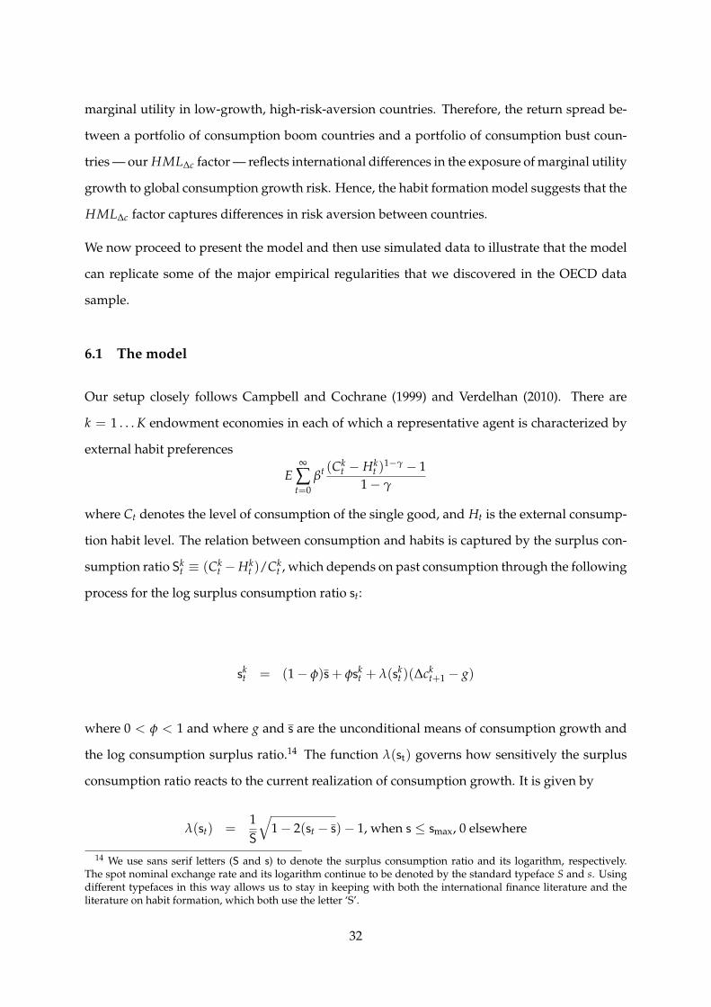
marginal utility in low-growth, high-risk-aversion countries. Therefore, the return spread be-

tween a portfolio of consumption boom countries and a portfolio of consumption bust coun-

tries — our HML∆c factor — reflects international differences in the exposure of marginal utility

growth to global consumption growth risk. Hence, the habit formation model suggests that the

HML∆c factor captures differences in risk aversion between countries.

We now proceed to present the model and then use simulated data to illustrate that the model

can replicate some of the major empirical regularities that we discovered in the OECD data

sample.

6.1 The model

Our setup closely follows Campbell and Cochrane (1999) and Verdelhan (2010). There are

k = 1 . . . K endowment economies in each of which a representative agent is characterized by

external habit preferences

E∞

∑t=0

βt (Ckt − Hk

t )1−γ − 1

1− γ

where Ct denotes the level of consumption of the single good, and Ht is the external consump-

tion habit level. The relation between consumption and habits is captured by the surplus con-

sumption ratio Skt ≡ (Ck

t −Hkt )/Ck

t , which depends on past consumption through the following

process for the log surplus consumption ratio st:

skt = (1− φ)s+ φsk

t + λ(skt )(∆ck

t+1 − g)

where 0 < φ < 1 and where g and s are the unconditional means of consumption growth and

the log consumption surplus ratio.14 The function λ(st) governs how sensitively the surplus

consumption ratio reacts to the current realization of consumption growth. It is given by

λ(st) =1S

√1− 2(st − s)− 1, when s ≤ smax, 0 elsewhere

14 We use sans serif letters (S and s) to denote the surplus consumption ratio and its logarithm, respectively.The spot nominal exchange rate and its logarithm continue to be denoted by the standard typeface S and s. Usingdifferent typefaces in this way allows us to stay in keeping with both the international finance literature and theliterature on habit formation, which both use the letter ‘S’.

32

where S = σ√

γ1−φ−B/γ , smax = s+ (1− S

2)/2, and B = γ(1− φ)− (γ2σ2)/(S2

), and σ denotes

the standard deviation of consumption growth.

In this model, the coefficient of relative risk aversion of country k is given by−Ckt Ucc(t)/Uc(t) =

γ/Skt . Hence, if country k’s consumption is close to the habit level, the surplus consumption

ratio of country k is low, which implies that the representative agent of country k is highly risk

averse. In this model, the stochastic discount factor is given by

Mkt+1 = β

(St+1Ct+1

StCt

)−γ

= βexp{

−γ[g + (φ−1)(skt −s) + (1 + λ(sk

t ))(∆ckt+1−g)]

}

where g is the mean growth rate of consumption. The risk-free interest rate is rkt = r− B(sk

t − s)

with r = − ln(β) + γg − (γ2σ2)/(2S2).15 We follow Verdelhan (2010) and impose B < 0.

This implies that risk-free interest rates are procyclical; that is, higher in countries with higher

surplus consumption ratios.

We assume that consumption growth of country k follows an i.i.d. normal process.

∆ckt+1 = g + ξt+1 + uk

t+1 ξt+1 ∼ i.i.d. N(0, σ2glob), uk

t+1 ∼ i.i.d. N(0, σ2idio)

cov(ξt+1, ukt+1) = 0

At each point in time, the average growth rate g and the global shock to consumption growth

ξt+1 are common to all countries, whereas ukt+1 denotes country-specific shocks to consumption

growth. Concerning the variance of the global and the country-specific shocks, we assume

that σglob = σidio = σ/√

2. As we will discuss shortly, the presence of a global component in

consumption growth is important in explaining our results.

We assume that financial markets are complete, which implies that the change in the real ex-

change rate between two countries equals the ratio of the two countries’ marginal utility growth

rates or stochastic discount factors

Qkt+1

Qkt

=Mt+1

Mkt+1

15For details about the derivation of equation (11), the reader is referred to Campbell and Cochrane (1999) andVerdelhan (2010).

33

where Qkt is the real exchange rate measured in units of country k goods per one unit of the

home country good, so that an increase in Qk implies a depreciation of country k’s currency vis-

a-vis the home country. Taking logarithms and substituting in from above for the logarithmic

pricing kernel, we obtain the rate of change of the real exchange rates

∆qkt+1 = κt + γ(1 + λ(sk

t ))(∆ckt+1 − g)− γ(1 + λ(st))(∆ct+1 − g) (11)

where κt summarizes all variables known at time t.

It is instructive to compare this condition for optimal risk sharing with the one obtained from

a model with constant relative risk aversion preferences without habit formation (see, e.g.,

Backus and Smith (1993) and Kollmann (1995)), which is given by the following.

∆qkt+1 = κt + γ(∆ck

t+1 − ∆ct+1)

The model without habit formation predicts that exchange rates move in lockstep with con-

sumption growth differences between countries. It is well known that this condition is grossly

violated in the data16. By contrast, in the habit model, whether the real exchange rate appreci-

ates or depreciates will not only depend on current differences in consumption growth between

countries. Rather, past differences will matter as well, because they are reflected in differences

in the surplus consumption ratio between the two countries. Specifically, if countries differ in

their consumption histories, the real exchange rate will change even if both countries experi-

ence the same consumption shock ∆ckt+1 = ∆ct+1 6= 0: because the sensitivity function λ(s) is

low when surplus consumption is high, the country with the higher surplus and, therefore, the

higher average consumption over the recent past will experience an appreciation if the common

consumption shock is positive, or a depreciation if the shock is negative. The reason for this is

that risk aversion in the high-surplus (low-λ) country is low and that marginal utility growth is

less exposed to the common consumption shock. Optimal risk sharing entails that purchasing

power is redistributed to the high-risk-aversion country in periods when both countries are hit

by the same negative consumption growth shock.

16[ad references]

34

Hence, in the habit model, countries differ in their exposure of marginal utility growth to the

same common shock. These differences in exposure to common shocks are also the source of

the currency risk premium in this model, which is given by the following.17

E(rxkt+1) = rk

t − rt − Et(∆qkt+1) =

γ2σ2

S2 (sk

t − st) (12)

Equation (12) shows that currencies of consumption boom countries generate positive expected

excess returns. This risk premium compensates for a likely depreciation of the currency in times

of low aggregate consumption growth. As we show in our simulations, sorting currencies on

past consumption growth is very similar to sorting them on their surplus consumption ratio.

To allow this intuition to extend to portfolios — as our empirical results suggest it does —

consumption growth must therefore have a common (global) component that does not wash

out in sufficiently large portfolios of currencies. To see this, average equation (11) over a subset

of I ⊂ {1....K} of our K currencies. If the number of elements in I, denoted here by #I, is

sufficiently large, we get the following.

1#I ∑

k∈I∆qk

t+1 = κt + γ

(1#I ∑

k∈I(1 + λ(sk

t ))

)ξt+1 − γ(1 + λ(st))(∆ct+1) (13)

Specifically, forming portfolios by sorting currencies on their past consumption growth and

assuming that there are many currencies in each of the consumption-growth-sorted portfolios,

the stochastic component of the returns described by our consumption carry factor HML∆c is

determined by changes in the average rate of change in the real exchange rate between high-

and low-consumption-growth currencies, given by

∆qhlt+1 = kt + γ[λh

t − λlt]ξt+1 (14)

where λht and λl

t are the average values of the sensitivity function of high h and low l surplus

consumption ratio country portfolios. Exchange rate changes between large portfolios of cur-

rencies are therefore solely driven by differences in the exposure to global consumption risk:

portfolios of currencies from countries with high surplus consumption ratios — which recently

17for further details, see Campbell and Cochrane (1999) and Verdelhan (2010)

35

have experienced a series of high consumption growth rates — appreciate if positive global

consumption growth shocks occur, and depreciate if the global shock turns out to be nega-

tive. The reason is that marginal utility in countries with high surplus consumption (low risk

aversion) has lower exposure to global consumption risk than countries with high risk aver-

sion. Optimal risk sharing therefore entails that wealth is redistributed to high-risk-aversion

countries when there are negative global shocks.

6.2 Calibration and results

We assume that all countries share the same set of parameters. The risk-aversion parameter γ

is set equal to 2, which corresponds to the value chosen by Campbell and Cochrane (1999) and

Verdelhan (2010). We estimate the average consumption growth rate g and its standard error σ

from the OECD data sample used in the main analysis of this study. Taking sample means over

all 33 countries, we find that the quarterly consumption growth rate corresponds to g = 0.52%,

and its standard deviation is σ = 1.1%. This implies a standard deviation of the global shock

and the country-specific shock of σglob = σidio = σ/√

2 = 0.81. The country-specific endow-

ment shocks ukt+1, which all have variance σidio, are uncorrelated across countries, but there is a

common consumption growth shock in all countries’ consumption growth rate ξt+1 with vari-

ance σglob. The quarterly real risk-free interest rate is set equal to r = 0.24%, which corresponds

to the average real US T-bill rate measured over the period from the first quarter of 1990 to

the fourth quarter of 2010. T-bill rates and consumer price inflation are obtained from the IFS

data tape18. As in Verdelhan (2010), we set B = −0.01. The persistence parameter φ is chosen

eventually such that the mean value of the consumption carry factor HML∆c approximately

corresponds to its sample counterpart; using real returns to calculate the consumption carry

factor from our OECD data sample, we find that HMLreal∆c,t+1 = 3.6% per year. For φ = 0.985,

the simulated consumption carry factor pays an average return of about this size. These pa-

rameter values imply that β = 0.99, S = 0.11 and Smax = 0.18. All parameter values are thus

close to the values chosen by Campbell and Cochrane (1999) and Verdelhan (2010), and Table

(8) presents an overview of the chosen parameter values.

With these parameters and 10 000 endowment shocks, we generate data and build currency

18US T-bill rates correspond to line 11160C...ZF, and consumer price inflation is calculated from 11164...ZF... .

36

Table 8: Habit model, parameter values

this paper Campbell and Cochrane(1999)

Verdelhan (2010)

calibrated parameters

g(%) 0.52 0.74 0.53σ(%) 1.1 0.75 0.51σidio(%) 0.81 - -σglob(%) 0.81 - -r(%) 0.24 0.23 0.34γ 2.00 2.00 2.00φ 0.99 0.97 0.99B −0.01 - −0.01ρ - 0.15

implied parametersβ 0.99 0.97 1.00S 0.11 0.06 0.07Smax 0.18 0.09 0.12

This table presents the parameters of the habit formation model outlined in section (6) and their chosen values inthis paper, in Campbell and Cochrane (1999) and in Verdelhan (2010). The data is at quarterly frequency. For thispaper, the reference period is 1990(1)-2010(4) (1947-1995 in Campbell and Cochrane (1999) and 1947(2)-2004(4) inVerdelhan (2010)). The average consumption growth rate g and its standard error σ are estimated from the OECDdata sample used in the main analysis of this study. The standard error of consumption growth σ is decomposedinto a global and an idiosyncratic component such that σglob = σidio = σ/

√2, whereby we assume that country-

specific and global consumption growth shocks are uncorrelated. The quarterly real risk-free rate correspondsto the average real U.S. T-bill rate over the reference period and it is sourced from the IFS data tape (US T-billrates corresponds to line 11160C..ZF, and consumer price inflation is calculated from 11164...ZF...). The persistenceparameter φ is chosen such that the mean value of the consumption carry factor HML∆c approximately correspondsto its sample counterpart; using real returns to calculate the consumption carry factor from our OECD data sample,we find HMLreal

∆c,t+1 = 3.6% per year. In Verdelhan (2010), ρ corresponds to the correlation of each simulatedcountries consumption growth shocks.

37

portfolio returns, the dollar risk factor rx as well as the consumption carry factor HML∆c. In

analogy to the empirical analysis in this study, we generate data for 33 countries and then sort

countries into six portfolios according to their consumption growth rates over the previous

four quarters. Table (9) presents the moments for the currency portfolios that this simulation

delivers.

Simulated portfolios of countries that have recently experienced higher consumption growth

pay an investor who borrows in his home currency and invests in these portfolios’ higher on av-

erage returns. Furthermore, consumption boom countries have high surplus consumption ra-

tios, which translate into low risk aversion, and thus relatively smooth intertemporal marginal

rates of substitution in consumption. The more risk averse the investor is compared with the

average country in a particular currency portfolio — that is, the lower his surplus consump-

tion ratio is relative to the average portfolio surplus consumption ratio — the more exposed his

marginal utility will be to consumption growth shocks. Currencies of countries with high ex-

posure to global consumption growth shocks will therefore appreciate when a negative global

consumption shock occurs. This reflects optimal risk sharing: the exchange rate appreciation

redistributes purchasing power to the high-risk-aversion, high-marginal- utility country in re-

cessions.

As carry trade returns are procyclical and thus risky, the investor demands a higher risk pre-

mium for investment into portfolios with higher surplus consumption ratios. Against the back-

ground of this model, we can therefore interpret our sorting of countries into portfolios accord-

ing to their recent consumption growth rates as sorting countries on their surplus consumption

ratios or risk aversion, and portfolios with higher past consumption growth rates expose the

investor to more home and global consumption growth risk. This explains why consumption

boom currencies pay higher expected returns.

Equation (14) suggests that within the framework of the consumption habit model outlined

above, our consumption carry factor HML∆c should mirror global risk only, and it should be

high if consumption growth is globally high and low otherwise. In the simulation with 33

countries and 10 000 global and country-specific endowment shocks, the correlation between

the global consumption growth shock ξt+1 and HML∆c equals about 0.4. This correlation is

not perfect because with 33 countries, portfolios are not sufficiently large such that not all id-

38

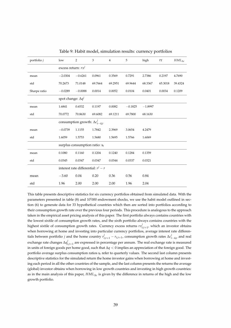
Table 9: Habit model, simulation results: currency portfolios

portfolio j low 2 3 4 5 high rx HML∆c

excess return: rxj

mean −2.0304 −0.6261 0.0961 0.3569 0.7291 2.7386 0.2197 4.7690

std 70.2673 71.0148 69.7664 69.2951 69.9644 68.3367 65.3018 39.4324

Sharpe ratio −0.0289 −0.0088 0.0014 0.0052 0.0104 0.0401 0.0034 0.1209

spot change: ∆qj

mean 1.6841 0.6532 0.1197 0.0082 −0.1825 −1.8997

std 70.0772 70.8630 69.6082 69.1211 69.7800 68.1630

consumption growth: ∆cjt−4,t

mean −0.0739 1.1155 1.7842 2.3969 3.0654 4.2479

std 1.6059 1.5753 1.5680 1.5695 1.5766 1.6069

surplus consumption ratio: st

mean 0.1080 0.1160 0.1204 0.1240 0.1284 0.1359

std 0.0345 0.0347 0.0347 0.0344 0.0337 0.0321

interest rate differential: rj − r

mean −3.60 0.04 0.20 0.36 0.56 0.84

std 1.96 2.00 2.00 2.00 1.96 2.04

This table presents descriptive statistics for six currency portfolios obtained from simulated data. With theparameters presented in table (8) and 10′000 endowment shocks, we use the habit model outlined in sec-tion (6) to generate data for 33 hypothetical countries which then are sorted into portfolios according totheir consumption growth rate over the previous four periods. This procedure is analogous to the approachtaken in the empirical asset pricing analysis of this paper. The first portfolio always contains countries withthe lowest sixtile of consumption growth rates, and the sixth portfolio always contains countries with thehighest sixtile of consumption growth rates. Currency excess returns rxj

t,t+1, which an investor obtainswhen borrowing at home and investing into particular currency portfolios, average interest rate differen-tials between portfolio j and the home country rj

t,t+1 − rt,t+1, consumption growth rates ∆cjt−4,t and real

exchange rate changes ∆qjt,t+1 are expressed in percentage per annum. The real exchange rate is measured

in units of foreign goods per home good, such that ∆q < 0 implies an appreciation of the foreign good. Theportfolio average surplus consumption ratios st refer to quarterly values. The second last column presentsdescriptive statistics for the simulated return the home investor gains when borrowing at home and invest-ing each period in all the other countries of the sample, and the last column presents the returns the average(global) investor obtains when borrowing in low growth countries and investing in high growth countries:as in the main analysis of this paper, HML∆c is given by the difference in returns of the high and the lowgrowth portfolio.

39

iosyncratic endowment shocks ukt+1 average out. Increasing the number of countries in the

simulation increases this correlation, and for K = 66 countries, it equals about 0.7.

The simulated consumption carry factor HML∆c is a globally priced risk factor, whereas the

mean currency return factor rx is not. Table (10) presents results from estimating the asset

pricing model of Section (5) again, but instead of using the data from our sample of 33 OECD

countries, test assets and pricing factors are constructed from simulated data. The habit model

with the parameter values specified above generates the stylized facts that we described for the

OECD data sample: country portfolio returns covary more strongly with the global recession

factor HML∆c the higher their consumption growth rate has been recently, and the risk factor

HML∆c is globally priced whereas the level factor rx is not.

7 Robustness checks

We perform several robustness checks. First, we estimate the asset pricing model using data

that span the period from the first quarter of 1990 to the fourth quarter of 2006, which omits the

years of the recent global financial crisis. Shortening the data sample does not fundamentally

change our findings. The results from this exercise are presented in Tables (24) to (26) in the

Appendix.

Second, we estimate the model with alternative base currencies. Using the Swiss franc, the

Canadian dollar, the British Pound, the Norwegian krone or the Australian dollar as base cur-

rencies, we obtain very similar results to those using the US dollar. Results for the Swiss franc

are especially nice and are presented in tables (18) to (20) in the Appendix.

Third, we sort currencies into portfolios according to their β with respect to our consumption

carry trade factor HML∆c. To do so, we estimate the following regression for each currency k

separately over rolling windows of 20 quarters.

rxkt,t+1 = ak + βk

1 · rxt,t+1 + βk2 · HML ∆ct,t+1 + εk

t,t+1 (15)

Hence, to obtain estimates βk2,t, we run regression (15) using time series that span the preced-

ing 20 quarters; i.e. the quarters from t − 19 to t. Because of this rolling window estimation

40

Table 10: Habit model, asset pricing results using simulated data

Panel A: risk prices and factor loadings

λrx λHML ∆c brx bHML ∆c

OLS estimate 0.0005 0.0115∗∗∗ 0.0235 1.1865∗∗∗

standard error (0.0016) (0.0010) (0.0605) (0.1025)

pricing error test 0.00 0.00

R2 0.89 0.89

Panel B: time series regression

aj βjrx β

jHML ∆c R2

low −0.0051∗∗∗ 0.9949∗∗∗ −0.5722∗∗∗

(0.0003) (0.0026) (0.0044) 0.96

2 −0.0016∗∗∗ 1.0104∗∗∗ 0.0116∗

(0.0006) (0.0053) (0.0082) 0.86

3 0.0002 0.9996∗∗∗ 0.0311∗∗∗

(0.0006) (0.0049) (0.0077) 0.88

4 0.0009∗ 0.9951∗∗∗ 0.0514∗∗∗

(0.0006) (0.0052) (0.0080) 0.88

5 0.0018∗∗∗ 1.0073∗∗∗ 0.0792∗∗∗

(0.0006) (0.0050) (0.0073) 0.89

high 0.0068∗∗∗ 0.9949∗∗∗ 0.4278∗∗∗

(0.0003) (0.0026) (0.0044) 0.96

This table shows estimates and standard errors obtained from running the same asset pricing exercise as in the empirical analysisof this paper, but instead of the OECD data set, simulated data are used. From the habit model outlined in section (6) and 10000 endowment shocks, data for 33 hypothetical countries have been constructed, and at each point in time, countries have beensorted into six portfolios according to their consumption growth rates realized over the preceding four periods. Test asset returnsare the returns a home investor obtains each period by borrowing at home and investing in the different portfolios.Panel A shows estimates and standard errors obtained from running the following time series regression for each currency port-folio j separately:

rxjt,t+1 = aj + β

j1 · rxt,t+1 + β

j2 · HML ∆ct,t+1 + ε

jt,t+1

In panel B, the first two columns report results from estimating the following cross-sectional regression using GMM:

E(rxj) = βjrx · λrx + β

jHML ∆c · λHML ∆c + αj

The third and the fourth columns show results from estimating the following cross-sectional regression:

E(rxj) = cov(rx, rxj) · brx + cov(HML ∆c, rxj) · bHML ∆c + αj

where again, covariances and factor loadings b have been estimated jointly using GMM. R2 measures are obtained as described

in the notes below table (3). The pricing error test reports the p-value for the null that the pricing errors jointly are zero.

41

procedure, the first five years are lost, such that the analysis covers the period from 1995(1) to

2010(4). Table (27) in the Appendix reveals that portfolios of currencies with a high βk2, i.e. cur-

rencies that at a given point in time load heavily on the risk factor HML∆c, pay higher returns

on average and have experienced higher consumption growth rates over the preceding year.

This confirms our result that high-consumption-growth currency portfolios are more exposed

to global risk than low-consumption-growth portfolios.

Finally, we repeat the estimations from the main body of the paper based on exchange rate

changes instead of excess returns. This, again, did not affect our main conclusions, suggesting

that we are truly pricing exchange rate risk and not movements in interest rate differentials.

8 Summary and conclusion

In this paper, we have suggested a new, consumption-based factor for pricing currency returns.

Our factor, which we refer to as the consumption carry factor or HML∆c, is based on sorting

currencies into portfolios based on past consumption growth and reflects the excess return of

borrowing in countries with the lowest consumption growth in the world over the past year

(bust countries) and investing in the currencies of countries that have experienced relative con-

sumption booms over the last year. HML∆c is a global risk factor in the sense that it successfully

explains the world cross section of currencies — for portfolios sorted on either past consump-

tion growth or on forward discounts as well as for individual currency pairs. In fact, we show

that currencies with high past consumption growth trade at high forward discounts, so that

countries with consumption booms appreciate much more than uncovered interest parity (UIP)

would imply, whereas countries with consumption busts appreciate by less than is implied by

UIP. These excess returns on consumption boom currencies are a compensation for the higher

exposure of these currencies with respect to our global factor: high-consumption-growth cur-

rencies depreciate more during times of aggregate distress, exposing investors to global risk.

The consumption carry factor HML∆c is as effective as other, purely financial factors that have

been proposed in the recent literature.

Our results are built on minimal theoretical restrictions and, in particular, are free of any specific

assumptions about preferences. They therefore provide strong independent evidence that risk

42

associated with longer- to medium-term movements in consumption are a key driver of the

cross section of currency returns. While our results are preference free, we showed that they

can be interpreted in the context of a consumption-based habit formation model. In the habit

model, sorting currencies on past consumption growth is akin to sorting countries according to

their risk aversion: consumption boom (bust) countries have high surplus consumption ratios

and low (high) risk aversion. Global consumption shocks therefore load more (less) strongly

on marginal utility in consumption bust (boom) countries, and optimal risk sharing requires

that these currencies should appreciate (depreciate) in worldwide downturns — as we find in

the data.

43

References

Baba, Naohiko, Yuji Sakurai , and Frank Packer, 2012, Foreign Exchange Futures, Forwards,

and Swaps, in Jessica James, Ian W. Marsh and Lucio Sarno, eds. Handbook of Exchange Rates

(John Wiley & Sons, New Jersey).

Backus, David K, and Gregor W. Smith, 1993, Consumption and real exchange rates in dynamic

economies with non-traded goods, Journal of International Economics 35, 279-316.

Bansal, Ravi, and Amir Yaron, 2004, Risks for the long run: A potential resolution of asset

pricing puzzles, Journal of Finance 59, 1481-1509.

Brunnermeier, Markus, K., Stefan Nagel, and Lasse H. Pedersen, 2008, Carry trades and cur-

rency crashes, Working paper, National Bureau of Economic Research.

Burnside, Craig, Martin Eichenbaum, Isaac, Kleshchelski, and Sergio Rebelo, 2011, Do peso

problems explain the returns to the carry trade? Review of Financial Studies 24, 853-891.

Campbell, John Y., and John H. Cochrane, 1999, By force of habit: A consumption-based expla-

nation of aggregate stock market behavior, Journal of Political Economy 107, 205-251.

Christiansen, Charlotte, Angel Ranaldo, and Paul Soderlind, 2001, Time varying systematic

risk of carry trade strategies, Journal of Financial and Quantitative Analysis 46, 1107-1125.

Cochrane, John H, 2005, Asset Pricing (Princeton University Press, Princeton).

Colacito, Riccardo, and Mariano M. Croce, 2011, Risks for the long run and the real exchange

rate, Journal of Political Economy 119, 153-181.

Engle, Charles, 1996, The forward discount anomaly and the risk premium: A survey of recent

evidence, Journal of Empirical Finance 3, 123-192.

Fama, Eugene F., 1984, Forward and spot exchange rates, Journal of Monetary Economics 14,

319-338.

Fama, Eugene F., and Kennet R. French, 1989, Business conditions and expected returns on

stocks and bonds, Journal of Financial Economics 25, 23-49.

Fama, Eugene F., and Kenneth R. French, 1993, Common risk factors in the returns of stocks

and bonds, Journal of Financial Economics 33, 3-56.

Habib, Maurizio M., and Livio Stracca, 2011, Getting beyond carry trade: what makes a safe

haven currency? Working paper, European Central Bank.

Jagannathan, Ravi, and Yong Wang, 2007, Lazy investors, discretionary consumption, and the

cross-section of stock returns. Journal of Finance 62, 1623-1661.

Jorda, Oscar, and Alan M. Taylor, 2009, The carry trade and fundamentals: Nothing to fear but

the feer itself, Working paper, National Bureau of Economic Research.

King, Michael R., Carol Osler, and Dagfinn Rime, 2011, Foreign exchange market structure,

players, and evolution, Working paper, Norges Bank.

Kollmann, Robert, 1995, Consumption, real exchange rates and the structure of international

asset markets, Journal of International Money and Finance 14, 191-2011.

Lettau, Martin, and Sidney Ludvigson, 2001, Resurrecting the (C)CAPM: A cross-sectional test

when risk premia are time-varying, Journal of Political Economy 109, 1238-1287.

Lewis, Karen K.,1995, Puzzles in international financial markets in Gene M. Grossmann and

Kenneth Rogoff, eds. Handbook of International Economics 3, 1913-1971 (Elsevier, North-Holland,

Amsterdam, New York and Oxford).

Lustig, Hanno N., and Adrien Verdelhan, 2007, The cross section of foreign currency risk pre-

mia and consumption growth risk, American Economic Review 97, 89-117.

Lustig, Hanno N., Nikolai L. Roussanov, and Adrien Verdelhan, 2011, Common risk factors in

currency markets, The Review of Financial Studies 24, 3731-3777.

Menkhoff, Lukas, Lucio Sarno, Maik Schmeling, and Andreas Schrimpf, 2012, Carry trades and

global foreign exchange volatility, Journal of Finance 67, 681-718.

Newey, Withney K., and Kenneth D. West, 1987, A simple, semi-definite, heteroscedasticity and

autocorrelation consistent covariance matrix, Econometrica 55, 703-708.

Nozaki, Masahiro, 2010, Do currency fundamentals matter for currency speculators? Working

Paper, International Monetary Fund.

Parker, Jonathan A., and Christian Julliard, 2005, Consumption risk and the cross section of

expected returns, Journal of Political Economy 113, 185-222.

Ranaldo, Angelo, and Paul Soderlind, 2010, Safe haven currencies, Review of Finance 14, 385-

407.

Verdelhan, Adrien, 2010, A habit-based explanation of the exchange rate risk premium, The

Journal of Finance 65, 123-146.

Verdelhan, Adrien, 2011, The Share of Systematic Risk in Bilateral Exchange Retes, Working

Paper, Massachusetts Institute of Technology.