we are on the way: analysis of on-demand ride-hailing...

Vol. 00, No. 0, Xxxxx 0000, pp. 000–000

issn 0000-0000 |eissn 0000-0000 |00 |0000 |0001

We Are on the Way: Analysis of On-Demand Ride-Hailing

Systems

Guiyun FengDepartment of Industrial and Systems Engineering, University of Minnesota, Minneapolis, MN 55455, [email protected]

Guangwen KongDepartment of Industrial and Systems Engineering, University of Minnesota, Minneapolis, MN 55455, [email protected]

Zizhuo WangDepartment of Industrial and Systems Engineering, University of Minnesota, Minneapolis, MN 55455, [email protected]

Recently, there has been a rapid rise of on-demand ride-hailing platforms, such as Uber and Didi, which allow

passengers with smartphones to submit trip requests and match them to drivers based on their locations and

drivers’ availability. This increased demand has raised questions about how such a new matching mechanism

will affect the efficiency of the transportation system, in particular, whether it will help reduce passengers’

average waiting time compared to traditional street-hailing systems.

In this paper, we address this question by building a stylized model of a circular road and comparing

the average waiting times of passengers under various matching mechanisms. After identifying key tradeoffs

between different mechanisms, we find that surprisingly, the on-demand matching mechanism could result

in higher or lower efficiency than the traditional street-hailing mechanism, depending on the parameters of

the system. To overcome the disadvantage of both systems, we further propose adding response caps to the

on-demand hailing mechanism and develop a heuristic method to calculate a near-optimal cap. We also test

our model using more complex road networks to show that our key observations still exist.

Keywords: on-demand ride-hailing; queueing systems; matching mechanism

1. Introduction

In the past few years, with the growth of information technology, we have witnessed the rapid

rise of on-demand ride-hailing platforms such as Uber, Lyft and Didi. Thanks to these platforms,

passengers nowadays can request rides using their smartphones instead of hailing taxis on the

streets, which used to be the norm in big metropolitan areas. Ride-hailing platforms help connect

passengers with drivers (private drivers and traditional taxi drivers) in real time. The growth of

these platforms has been astonishing: Uber completed its two-billionth trip in July 2016 (Hawkins

2016b), Didi was responsible for 1.43 billion trips in 2015 alone (Hawkins 2016a), and the growth

continues to accelerate.

Despite the rapid growth, policy makers worldwide continue to debate about whether such

1

2

platforms should be encouraged, and if so, to what extent. Prominent in the debate are concerns

about safety, privacy and liability of the drivers and the platform (Rogers 2015). Yet there is also

the central question of whether these platforms always increase convenience for passengers and the

efficiency of the transportation system. In particular, policy makers struggle to understand how

much increased efficiency, if any, such platforms bring to the transportation system; whether the

platform can reduce passengers’ average waiting times when they need a ride, and if the platform

has negative effects on the transportation system. Understanding the answers to these questions

would enable policy makers to make more informed decisions when enacting regulations for this

emerging service paradigm.

Unfortunately, the answers to these questions are not obvious. Even though it is generally

believed that such platforms may help people obtain transportation more efficiently, it is also

realized that a platform may decrease the efficiency of transportation during rush hour when the

supply easily matches the demand even without the use of ride-sharing platforms. In particular,

in a high-traffic situation, it is likely that a driver heading to pick up a passenger who requested

service from a platform would encounter another passenger en route, thus increasing the otherwise

shorter pickup time and resulting in a loss of efficiency. For example, Steinberg (2012) points out

that “People waiting on Manhattan’s Fifth Avenue in the middle of rush hour don’t need an app

to tell cabs to come to the area.” An example of action taken in response to such situations is

the Shanghai government’s 2014 ban on the use of on-demand riding platforms during peak traffic

hours (from 7:30 AM to 9:30 AM and from 6:30 PM to 8:30 PM). Although the ban was lifted,

the question remains regarding when these platforms tend to increase or decrease the efficiency of

the system.

This research attempts to shed light on this question from an operations point of view. Specif-

ically, we consider a stylized model in which taxis1 drive on a circular road, and we study the

performance of different demand-matching mechanisms under the proposed model. Although highly

stylized, this model captures the main tradeoffs between the street-hailing system and the on-

demand hailing system and thus provides useful insights. In particular, for the street-hailing system,

we consider a corresponding “no-call mechanism,” in which no platform matches passengers with

taxis, and arriving passengers are picked up by the first available taxi passing by. For the on-

demand hailing system, we consider a corresponding “call mechanism,” in which waiting passengers

1 In this paper, we use “taxis” to refer to the cars that are used to transport passengers. The term may includetraditional taxis, as well as private cars or even self-driving cars that are used to provide transportation services.

3

are matched to the nearest idle taxi whenever there are taxis available. We are interested in com-

paring the average waiting time of passengers using different mechanisms. To this end, we first

pinpoint the advantages and disadvantages of each mechanism. The advantage of the call mecha-

nism lies in its ability to tell the driver where (which direction) to go to pick up the next customer.

However, taxis using the call mechanism may suffer from the possibility of forgoing future better

matching opportunities when accepting an incoming request. Upon understanding these tradeoffs,

we illustrate the conditions under which one mechanism is more efficient than the other by using

an approximate M/M/k queue. Somewhat surprisingly, we show that the call mechanism is more

efficient (has lower average waiting time) when the traffic intensity is low or high, while the no-

call mechanism could be more efficient when the traffic intensity is in the middle range and when

the density of taxis distributed in the transportation system is low. This result, partly confirming

what people previously thought, provides new insights into when the call mechanism should be

encouraged and when it should not be.

Based on the tradeoffs between the two mechanisms, we further propose a modified call mecha-

nism that adds a distance cap such that a passenger is matched to a taxi only when the distance

is below the cap. We show that adding such a cap would preserve most of the benefit of the call

mechanism, while greatly diminishing the disadvantage, thus achieving a superior overall perfor-

mance. We further propose a heuristic to calculate a near-optimal cap that is shown to provide a

very good policy compared to the optimal selection.

Finally, we also test our conclusions using more complex grid networks. We find that although

the observed phenomenon could be less pronounced, it nevertheless remains. Therefore, we believe

that our results could be instrumental for decision makers to understand the tradeoffs of the new

service paradigm.

The remainder of the paper is organized as follows: In Section 2, we review the literature that is

related to this work. In Section 3, we introduce our models. In Section 4, we consider a simpler one-

direction system to illustrate main insights. Then we extend our discussion to a more realistic two-

direction system in Section 5. In Section 6, we propose to add a distance cap to the call mechanism

and study the optimal selection of the cap. In Section 7, we conduct numerical experiments on

more complex road networks. We conclude the paper in Section 8.

2. Literature Review

The emergence and popularity of the sharing economy in recent years have raised many interesting

research questions and attracted significant academic interest. The research conducted in this area

4

can be categorized into strategic and operational levels. In the following, we review literature in

both categories.

On the strategic level, several recent works examine how the emergence of the sharing econ-

omy changes the way people behave and subsequently its impact on the economy. For example,

Fraiberger and Sundararajan (2015) use aggregate data from the U.S. automobile industry to show

that a shift from ownership to collaborative consumption may lead to less usage, lower used-good

prices and a higher consumer surplus. Benjaafar et al. (2015) consider an equilibrium model that

endogenizes market friction and provide analytical results showing that product usage and own-

ership may increase with the presence of a sharing platform. Jiang and Tian (2016) examine the

impact of a product-sharing platform on the manufacturer’s profit and consumers’ surplus. They

find that when product quality is exogenous, the manufacturer and consumers are better off when

the marginal production cost is high, but both are worse off otherwise. However, when the product

quality is endogenous, the consumer surplus is always lower in the presence of a sharing platform. In

comparison to the research focusing on product sharing, our study considers operational decisions

in matching supply and demand of transportation service via on-demand hailing platforms and

studies the impact of different matching mechanisms. In addition, most papers consider consumer

surplus that depends on product price and quality. Instead, we focus on whether an on-demand

hailing platform can reduce average passenger waiting time.

Another growing stream of papers focus on the operational decision-making problems faced by

the on-demand service platforms. One problem that has been considered extensively is capacity

management via dynamic pricing. In particular, on-demand service platforms have enabled service

providers to choose their own flexible work schedules, presenting new challenges to managing the

service capacity. To address this problem, analysis often focuses on how the platform can adjust

agent payment and service price to efficiently allocate capacity. For example, Gurvich et al. (2015)

employ a newsvendor model to study the capacity management problem in sharing marketplaces

where workers have the flexibility to choose their own work schedules. Cachon et al. (2015) consider

several contractual forms ranging from fixed price/compensation to surge pricing under a two-

period framework and find that providers and consumers are generally better off with surge pricing.

Riquelme et al. (2015) model a ride-sharing platform as a queue with customers’ arrival and

the drivers’ work hours depending on the real-time dynamic service price, and they show that

the platform cannot significantly increase its revenue by using a dynamic pricing policy based

on a threshold number of drivers. Taylor (2016) examines how two defining features of an on-

demand service platform – congestion-driven delay disutility and agent independence – affect the

5

platform’s optimal per-service price and wage. Tang et al. (2016) use the steady-state equilibrium

to characterize the optimal price, wage and payout ratio that maximize the profit of the platform,

where an M/M/1 queuing model is used to get the approximated waiting time for passengers. In

our paper, we do not focus on the pricing and capacity decisions. Instead, we assume the demand

and the supply are exogenously given and focus on comparing different matching mechanisms under

various utilization levels.

In addition to capacity management, another important operational problem faced by platforms

is how to efficiently match service providers with customers. Several recent works have taken on

this task. Allon et al. (2012) explore the role of the platforms in facilitating information gathering,

operational efficiency and communication by considering three different market models employed by

platforms and then characterize the corresponding market outcomes. Cullen and Farronato (2014)

study the problem of balancing highly variable demand and supply for a frictional matching market

and calibrate their model by using data from TaskRabbit. Anderson et al. (2015) investigate timely

exchanges for agents in a barter marketplace, and their results show that a greedy policy that

attempts to match upon each arrival is approximately optimal (minimizes average waiting time)

among a large class of policies including batching policies. Baccara et al. (2015) consider two-sided

matching with vertically different preferences over agents. They show that the optimal mechanism

always matches congruent pairs immediately and holds on to a stock of incongruent pairs up to a

certain threshold, and a centralized market is more appealing than the corresponding decentralized

one. Akbarpour et al. (2016) study different dynamic matching strategies in network markets where

agents arrive stochastically and stay for a random period of time before leaving the system if not

matched. They show that waiting to thicken the market is highly valuable if the central planner

knows the agents’ departure time, otherwise, a greedy local algorithm is close to optimal. Hu and

Zhou (2016) model dynamic matching between the demand and supply of heterogeneous types in

a periodic-review fashion. They provide sufficient conditions on matching rewards such that the

optimal matching policy follows a priority hierarchy among possible matching pairs. Similar to

these works, the on-demand matching problem studied in our work is also a two-sided dynamic

matching problem faced by a centralized platform; in particular, we can model the preference level

(matching quality) for any taxi-passenger pair by their distance. However, it would be challenging

to use the methods in these papers to evaluate the efficiency of the system. This is because a

key differentiating factor in our paper is that since taxis keep moving, the matching scores are

constantly evolving even when no new arrival occurs. We obtain insights that are particular to this

dynamic.

6

In addition to the operations management literature, the dynamic matching problem described

above has also been studied in the transportation literature under the taxi fleet dispatch con-

text. For example, Meyer and Wolfe (1961) provide approximate stationary analysis for different

dispatch systems, providing explicit expressions for operational decisions. McLeod (1972) develop

performance models for the taxi system based on queueing theory and show the important tradeoffs

between passenger waiting time, fleet size and taxi productivity. Bailey and Clark (1992) study

the structure and behavior of an urban taxi system, where the average waiting time and taxi uti-

lization are presented for simulation models under different dispatch and idle-time strategies. In

this paper, we focus on comparing two matching strategies: street-hailing and on-demand hailing,

and we obtain insights about under what circumstances each strategy has better performance. We

also propose potential ways to eliminate the disadvantage of both strategies and thus improve the

efficiency of the system.

3. Models

We consider a stylized transportation system on a circular road with perimeter R. There are k

taxis in the system. Passengers arrive at the system according to a Poisson process with rate λ,

and their arrival locations are uniformly distributed on the circle. Each arriving passenger requests

a service with duration d, where d follows an exponential distribution with mean 1/µ.2 We assume

that all taxis have a constant speed of one; i.e., they travel one unit of distance on the circle in a

unit of time.

In this paper, we consider two different systems in terms of the direction of travel: a one-direction

system and a two-direction system. In the one-direction system, only a clockwise direction of travel

is allowed. That is, all taxis travel clockwise, and so are the passengers’ requests (i.e., if a passenger

requests a service with duration d, then she is requesting to be transported in a clockwise direction

for a distance of d). In contrast, in the two-direction system, taxis and passengers are allowed to

travel in both directions. More precisely, in the two-direction system, the initial direction of each

taxi, the requested service direction of each passenger, as well as the travel direction of a taxi

after completing a service, are all randomly chosen, with a 50% chance being clockwise and a 50%

chance being counterclockwise.

The focus of this paper is on comparing two matching mechanisms. The first mechanism is

referred to as the call mechanism, which is used to model the matching process made by the

2 In our model, it is possible for d to be greater than R. However, our model can be easily modified to one in whichthe requested durations of the passengers follow a bounded distribution.

7

on-demand ride-hailing platforms. In the call mechanism, when a passenger arrives, a platform

immediately matches the passenger to the nearest taxi if there is a taxi available; otherwise, arrived

passengers will wait until the next taxi becomes available, at which time the taxi will be matched

to its nearest passenger (the remaining passengers, if any, would keep waiting for the next taxi to

become available). Once a match between a taxi and a passenger is made, the taxi is committed

to serving that passenger next, and the passenger waits for the matched taxi to come. In the one-

direction system, the distance between a passenger and a taxi is defined as the distance for a taxi to

reach a passenger when driving clockwise; while in the two-direction system, the distance is defined

as the shorter distance between driving clockwise and counterclockwise. The other mechanism is

the no-call mechanism, which is used to model the matching process of traditional street hailing.

In the no-call mechanism, no matching occurs, and a passenger is picked up by the first available

taxi passing by.

To summarize, we consider four settings in this paper: one-direction call/no-call systems and

two-direction call/no-call systems. The features of the four settings are listed in Table 1.

Table 1 Features of call/no-call mechanisms in one-direction/two-direction systems

Transportation systems 1-d no-call 1-d call 2-d no-call 2-d callDriving direction Clockwise Clockwise Both BothInitial direction/

Request direction/ Clockwise Clockwise Random RandomDirection upon finish

Matched to Matched toMatching mechanism No matching nearest No matching nearest between

clockwise two directions

The goal of this work is to study and compare the efficiency of these systems, particularly call

versus no-call systems. We use the average waiting time of passengers as the performance measure,

which is defined as the average time interval between a passenger’s arrival and being picked up.

By Little’s Law, the average waiting time of passengers is proportional to the average number

of passengers waiting in the system. Thus, the average waiting time can measure the passenger’s

satisfaction and the congestion of the system.

4. One-Direction Call/No-Call Systems

In this section, we first study the one-direction systems. Through studying the one-direction sys-

tems, we illustrate the tradeoffs between the call and no-call mechanisms, which will be helpful

for studying the more complicated two-direction systems in Section 5. The approach of our study

8

is as follows: We first perform numerical experiments on these systems, which lead to some key

observations. Then, we provide intuitive explanations for those observations. Finally, we verify the

observations with theoretical analysis using a novel approximation approach.

4.1. Numerical Experiments

In the following, we perform numerical experiments about the one-direction systems. In each numer-

ical experiment, we fix the service rate µ, the number of taxis k, and the road length R, and we

adjust the arrival rate λ to see how the average waiting time of passengers changes with λ. Note

that this effectively changes the utilization level ρ.= λ/kµ, which is an indicator of the congestion

level of the system. In addition, without loss of generality, we fix µ= 0.1 throughout our study.3

Furthermore, we vary the values of k and R to see how these parameters affect the relation between

the average waiting time and the utilization level ρ.

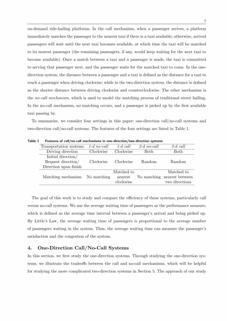
We start with the one-direction call system. The results are shown in Figure 1. From Figure 1,

we have the following observation.4

Observation 1. In the one-direction call system, the average waiting time is not always monoton-

ically increasing in ρ. In particular, it increases in ρ when ρ is small or large. However, it could

decrease in ρ when ρ is medium. Moreover, such non-monotonicity is more pronounced when R is

large.

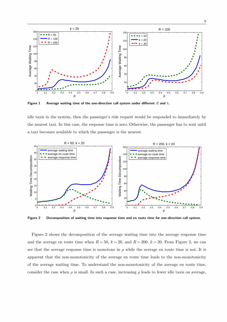
To understand the intuition behind the non-monotonicity observed in Figure 1, we decompose

the waiting time for one passenger into two components: response time and en route time. Here,

the response time is defined as the time between a passenger’s arrival and when the passenger’s ride

request is responded to by the nearest taxi, and the en route time is defined as the time between

the request response and the passenger pickup. In particular, when a passenger arrives, if there are

3 In our models, it is easy to see that a system with parameters (λ,µ, k,R) is equivalent to a system with parameters(cλ, cµ, k,R/c) except that the time scale is multiplied by 1/c, i.e., one unit of time in the original system becomes1/c unit of time in the new system. Therefore, we can fix one parameter among λ, µ and R in our study without lossof generality. In our paper, we choose to fix µ.

4 In all our simulation results, each average waiting time is based on the average of 500 replications of sample paths.In each sample path, we run the system from an idle state. Then we use the average waiting time between the t0-thand t1-th passengers as the average waiting time in that sample path. Here, t0 can be viewed as having a warm-upperiod until the system enters a steady state. The value of t0 is determined by a commonly used graphical method,see Welch (1983). In particular, let Yj denote the average waiting time of passenger j over 500 sample paths. Thenwe take w= 20 and let Yj = (1/w)

∑ji=j−w+1 Yi be the average waiting time between the (j−w+ 1)-th and the j-th

passengers. We plot Yj and observe visually when Yj becomes stable. Then we choose a t0 that is large enough sothat Yj has entered a steady state. We further choose t1 = t0 + 6000.

Also, we note that the observations in this section and Section 5 are obtained from extensive numerical experiments,and the figures we choose to show are representative of the numerical results. As we will show in Sections 4.2 and5.2, these observations are generally valid in an approximation system.

9

0 0.1 0.2 0.3 0.4 0.5 0.6 0.7 0.8 0.90

20

40

60

80

100

120

140

160k = 20

Ave

rage

Wai

ting

Tim

e

ρ

R = 50R = 100R = 200

0 0.1 0.2 0.3 0.4 0.5 0.6 0.7 0.8 0.90

20

40

60

80

100

120

140

ρ

Ave

rage

Wai

ting

Tim

e

R = 100

k = 10k = 20k = 30

Figure 1 Average waiting time of the one-direction call system under different R and k.

idle taxis in the system, then the passenger’s ride request would be responded to immediately by

the nearest taxi. In this case, the response time is zero. Otherwise, the passenger has to wait until

a taxi becomes available to which the passenger is the nearest.

0 0.1 0.2 0.3 0.4 0.5 0.6 0.7 0.8 0.90

5

10

15

20

25

30

35

40

45R = 50, k = 20

Wai

ting

Tim

e D

ecom

posi

tion

ρ

average waiting timeaverage en route timeaverage response time

0 0.1 0.2 0.3 0.4 0.5 0.6 0.7 0.8 0.90

20

40

60

80

100

120

140

160R = 200, k = 20

Wai

ting

Tim

e D

ecom

posi

tion

ρ


Figure 2 Decomposition of waiting time into response time and en route time for one-direction call system.

Figure 2 shows the decomposition of the average waiting time into the average response time

and the average en route time when R= 50, k = 20, and R= 200, k = 20. From Figure 2, we can

see that the average response time is monotone in ρ while the average en route time is not. It is

apparent that the non-monotonicity of the average en route time leads to the non-monotonicity

of the average waiting time. To understand the non-monotonicity of the average en route time,

consider the case when ρ is small. In such a case, increasing ρ leads to fewer idle taxis on average,

10

which means that the average distance between an arriving passenger and the nearest idle taxi

is longer, and thus, the en route time increases with ρ in this range. When ρ is high, a larger

ρ implies that, on average, more passengers are waiting for service in the system. Therefore, the

average distance between the taxi and the nearest passenger decreases in ρ; thus the en route time

decreases in ρ. When ρ is in the middle range (near where the en route time peaks), a passenger

arriving at the system is likely to find him/herself among the few waiting passengers, and at the

same time, not more than one taxi is available. In this case, the average distance between the

passenger and the taxi is the largest, which explains the peak of the en route time. Moreover, this

effect is more significant when R is large, because the en route time will play a more significant

role in determining the total waiting time in that case. Therefore, the non-monotonicity is more

pronounced when R is large.

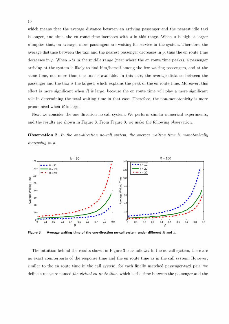
Next we consider the one-direction no-call system. We perform similar numerical experiments,

and the results are shown in Figure 3. From Figure 3, we make the following observation.

Observation 2. In the one-direction no-call system, the average waiting time is monotonically

increasing in ρ.

0 0.1 0.2 0.3 0.4 0.5 0.6 0.7 0.8 0.90

20

40

60

80

100

120

140

160

Ave

rage

Wai

ting

Tim

e

k = 20

ρ

R = 50

R = 100

R = 200

0 0.1 0.2 0.3 0.4 0.5 0.6 0.7 0.8 0.90

20

40

60

80

100

120

140

ρ

Ave

rage

Wai

ting

Tim

e

R = 100

k = 10k = 20k = 30

Figure 3 Average waiting time of the one-direction no-call system under different R and k.

The intuition behind the results shown in Figure 3 is as follows: In the no-call system, there are

no exact counterparts of the response time and the en route time as in the call system. However,

similar to the en route time in the call system, for each finally matched passenger-taxi pair, we

define a measure named the virtual en route time, which is the time between the passenger and the

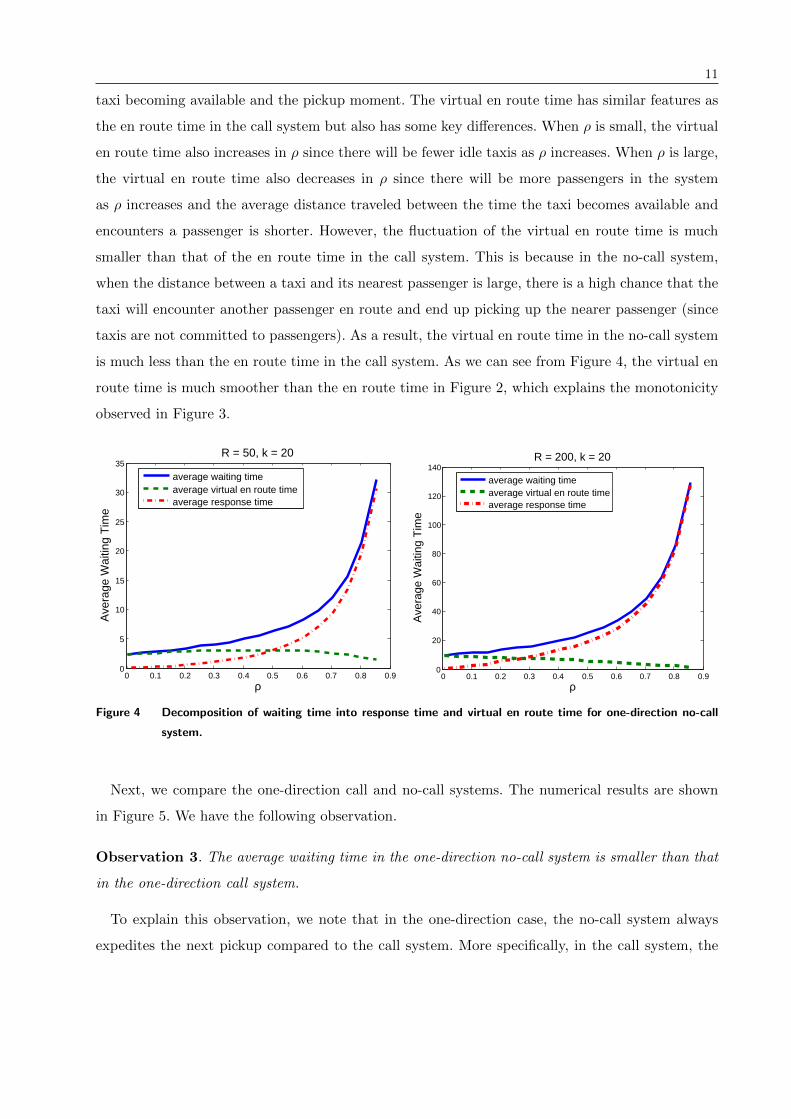
11

taxi becoming available and the pickup moment. The virtual en route time has similar features as

the en route time in the call system but also has some key differences. When ρ is small, the virtual

en route time also increases in ρ since there will be fewer idle taxis as ρ increases. When ρ is large,

the virtual en route time also decreases in ρ since there will be more passengers in the system

as ρ increases and the average distance traveled between the time the taxi becomes available and

encounters a passenger is shorter. However, the fluctuation of the virtual en route time is much

smaller than that of the en route time in the call system. This is because in the no-call system,

when the distance between a taxi and its nearest passenger is large, there is a high chance that the

taxi will encounter another passenger en route and end up picking up the nearer passenger (since

taxis are not committed to passengers). As a result, the virtual en route time in the no-call system

is much less than the en route time in the call system. As we can see from Figure 4, the virtual en

route time is much smoother than the en route time in Figure 2, which explains the monotonicity

observed in Figure 3.

0 0.1 0.2 0.3 0.4 0.5 0.6 0.7 0.8 0.90

5

10

15

20

25

30

35

ρ

Ave

rage

Wai

ting

Tim

e

R = 50, k = 20

average waiting timeaverage virtual en route timeaverage response time

0 0.1 0.2 0.3 0.4 0.5 0.6 0.7 0.8 0.90

20

40

60

80

100

120

140

ρ

Ave

rage

Wai

ting

Tim

e

R = 200, k = 20

average waiting timeaverage virtual en route timeaverage response time

Figure 4 Decomposition of waiting time into response time and virtual en route time for one-direction no-call

system.

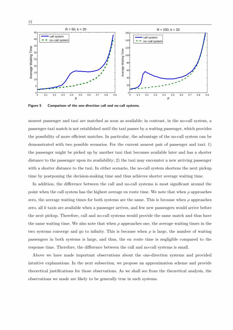
Next, we compare the one-direction call and no-call systems. The numerical results are shown

in Figure 5. We have the following observation.

Observation 3. The average waiting time in the one-direction no-call system is smaller than that

in the one-direction call system.

To explain this observation, we note that in the one-direction case, the no-call system always

expedites the next pickup compared to the call system. More specifically, in the call system, the

12

0 0.1 0.2 0.3 0.4 0.5 0.6 0.7 0.8 0.90

5

10

15

20

25

30

35

40

45A

vera

ge W

aitin

g T

ime

R = 50, k = 20

ρ

call systemno−call system

0 0.1 0.2 0.3 0.4 0.5 0.6 0.7 0.8 0.90

20

40

60

80

100

120

140

160

Ave

rage

Wai

ting

Tim

e

R = 200, k = 20

ρ


Figure 5 Comparison of the one-direction call and no-call systems.

nearest passenger and taxi are matched as soon as available; in contrast, in the no-call system, a

passenger-taxi match is not established until the taxi passes by a waiting passenger, which provides

the possibility of more efficient matches. In particular, the advantage of the no-call system can be

demonstrated with two possible scenarios. For the current nearest pair of passenger and taxi: 1)

the passenger might be picked up by another taxi that becomes available later and has a shorter

distance to the passenger upon its availability; 2) the taxi may encounter a new arriving passenger

with a shorter distance to the taxi. In either scenario, the no-call system shortens the next pickup

time by postponing the decision-making time and thus achieves shorter average waiting time.

In addition, the difference between the call and no-call systems is most significant around the

point when the call system has the highest average en route time. We note that when ρ approaches

zero, the average waiting times for both systems are the same. This is because when ρ approaches

zero, all k taxis are available when a passenger arrives, and few new passengers would arrive before

the next pickup. Therefore, call and no-call systems would provide the same match and thus have

the same waiting time. We also note that when ρ approaches one, the average waiting times in the

two systems converge and go to infinity. This is because when ρ is large, the number of waiting

passengers in both systems is large, and thus, the en route time is negligible compared to the

response time. Therefore, the difference between the call and no-call systems is small.

Above we have made important observations about the one-direction systems and provided

intuitive explanations. In the next subsection, we propose an approximation scheme and provide

theoretical justifications for those observations. As we shall see from the theoretical analysis, the

observations we made are likely to be generally true in such systems.

13

4.2. Approximation Scheme

In this subsection, we propose an approximation scheme for the one-direction system studied

above. The approximation scheme is useful in several ways. First, it provides an efficient way to

obtain performance measures for such systems, rather than performing potentially burdensome

simulations. Second, it captures the key characteristics of different matching mechanisms and thus

allows us to obtain meaningful insights. As we will show, under the approximation scheme, we

can prove several insights we observed in the actual system. Moreover, the approximation scheme

allows extension to more complex settings, such as other road setups or matching mechanisms,

thus offering a powerful tool for analyzing such problems.

To establish the approximation scheme, we note that the transportation system shares some

similarities with a queueing system. In particular, taxis can be viewed as servers, while passengers

waiting for a ride can be viewed as customers waiting for service. The arrival rate of passengers and

the service rate of taxis are also similar to the counterparts in a queueing system. However, unlike

a queueing system where customers are served according to certain priority rules (e.g., first-come

first-served), in the transportation system, the locations of taxis and passengers play a key role

in determining the sequence of service. In addition, the waiting time for a passenger is not only

impacted by waiting for busy taxis to become available, but also affected by the time en route.

To incorporate these features, we define the extended service time in the transportation system,

which is the sum of the actual service time and the en route time. In our model, the service time is

exponentially distributed with mean 1/µ. However, the explicit distribution of the en route time is

hard to obtain. To address this issue, in the approximation scheme, we first compute an approximate

expected en route time for the next service, which we denote by te. We note that te is dependent

on the number of waiting passengers and available taxis in the system. Then we approximate the

extended service time by assuming that it follows an exponential distribution with mean 1/µ+ te.

Finally, with this approximation for the extended service time, we approximate the transportation

system by an M/M/k queue, in which arrivals form a single queue and are governed by a Poisson

process, and there are k servers with state-dependent service rates as previously described. In the

following, we specify the M/M/k approximations for the one-direction call/no-call systems.

For the one-direction call system, let n denote the total number of passengers in the system

(waiting for service or being served), and λ(1c)n and µ(1c)

n denote the arrival rate and the service rate

when there are n passengers in the system, respectively. By definition, λ(1c)n = λ for all n. In the

following, we calculate the average en route time in order to obtain µ(1c)n .

14

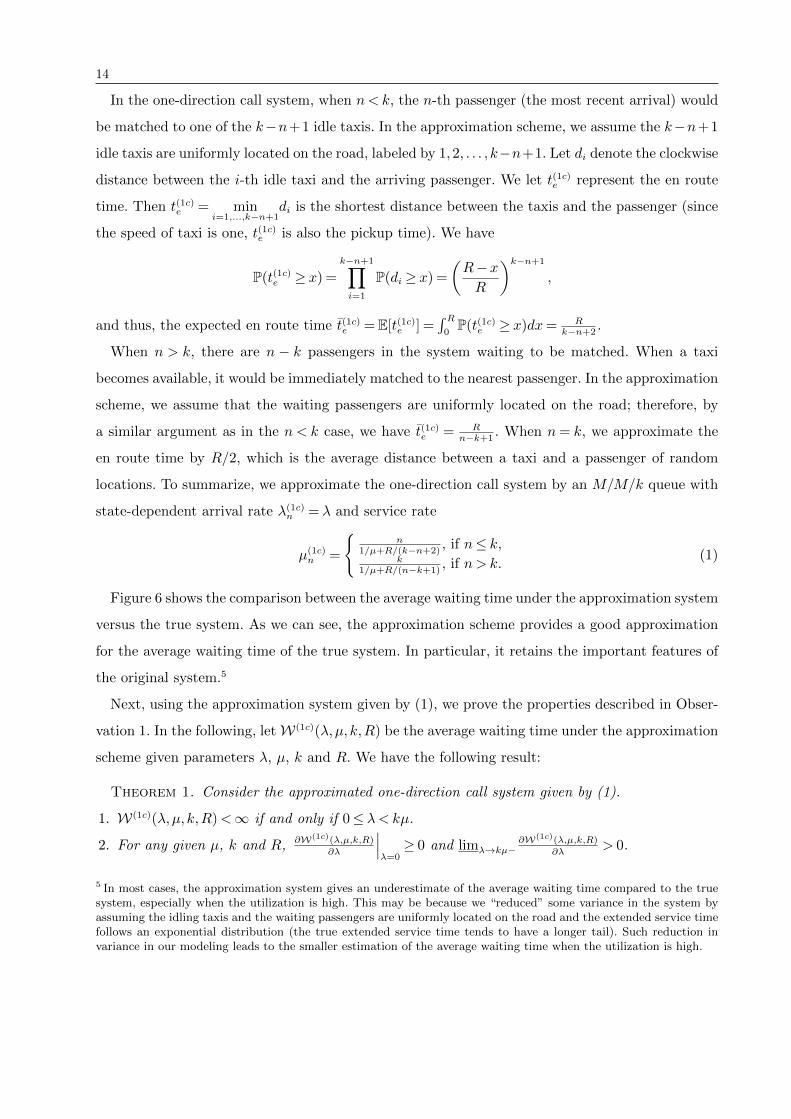
In the one-direction call system, when n< k, the n-th passenger (the most recent arrival) would

be matched to one of the k−n+1 idle taxis. In the approximation scheme, we assume the k−n+1

idle taxis are uniformly located on the road, labeled by 1,2, . . . , k−n+1. Let di denote the clockwise

distance between the i-th idle taxi and the arriving passenger. We let t(1c)e represent the en route

time. Then t(1c)e = mini=1,...,k−n+1

di is the shortest distance between the taxis and the passenger (since

the speed of taxi is one, t(1c)e is also the pickup time). We have

P(t(1c)e ≥ x) =k−n+1∏i=1

P(di ≥ x) =

(R−xR

)k−n+1

,

and thus, the expected en route time t(1c)e =E[t(1c)e ] =∫ R0P(t(1c)e ≥ x)dx= R

k−n+2.

When n > k, there are n − k passengers in the system waiting to be matched. When a taxi

becomes available, it would be immediately matched to the nearest passenger. In the approximation

scheme, we assume that the waiting passengers are uniformly located on the road; therefore, by

a similar argument as in the n < k case, we have t(1c)e = Rn−k+1

. When n= k, we approximate the

en route time by R/2, which is the average distance between a taxi and a passenger of random

locations. To summarize, we approximate the one-direction call system by an M/M/k queue with

state-dependent arrival rate λ(1c)n = λ and service rate

µ(1c)n =

{n

1/µ+R/(k−n+2), if n≤ k,

k1/µ+R/(n−k+1)

, if n> k.(1)

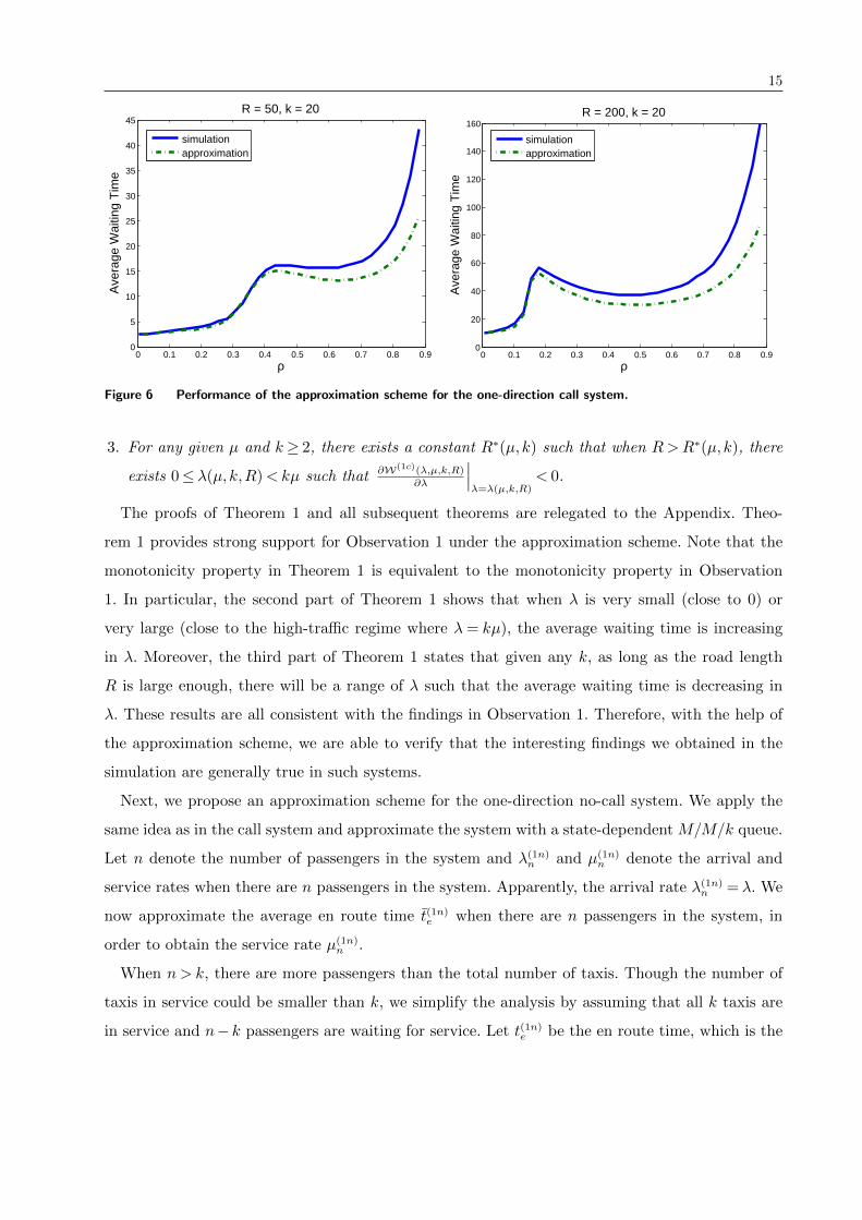
Figure 6 shows the comparison between the average waiting time under the approximation system

versus the true system. As we can see, the approximation scheme provides a good approximation

for the average waiting time of the true system. In particular, it retains the important features of

the original system.5

Next, using the approximation system given by (1), we prove the properties described in Obser-

vation 1. In the following, letW(1c)(λ,µ, k,R) be the average waiting time under the approximation

scheme given parameters λ, µ, k and R. We have the following result:

Theorem 1. Consider the approximated one-direction call system given by (1).

1. W(1c)(λ,µ, k,R)<∞ if and only if 0≤ λ< kµ.

2. For any given µ, k and R, ∂W(1c)(λ,µ,k,R)

∂λ

∣∣∣λ=0≥ 0 and limλ→kµ−

∂W(1c)(λ,µ,k,R)

∂λ> 0.

5 In most cases, the approximation system gives an underestimate of the average waiting time compared to the truesystem, especially when the utilization is high. This may be because we “reduced” some variance in the system byassuming the idling taxis and the waiting passengers are uniformly located on the road and the extended service timefollows an exponential distribution (the true extended service time tends to have a longer tail). Such reduction invariance in our modeling leads to the smaller estimation of the average waiting time when the utilization is high.

15

0 0.1 0.2 0.3 0.4 0.5 0.6 0.7 0.8 0.90

5

10

15

20

25

30

35

40

45

ρ

Ave

rage

Wai

ting

Tim

eR = 50, k = 20

simulationapproximation

0 0.1 0.2 0.3 0.4 0.5 0.6 0.7 0.8 0.90

20

40

60

80

100

120

140

160

ρ

Ave

rage

Wai

ting

Tim

e

R = 200, k = 20


Figure 6 Performance of the approximation scheme for the one-direction call system.

3. For any given µ and k≥ 2, there exists a constant R∗(µ,k) such that when R>R∗(µ,k), there

exists 0≤ λ(µ,k,R)<kµ such that ∂W(1c)(λ,µ,k,R)

∂λ

∣∣∣λ=λ(µ,k,R)

< 0.

The proofs of Theorem 1 and all subsequent theorems are relegated to the Appendix. Theo-

rem 1 provides strong support for Observation 1 under the approximation scheme. Note that the

monotonicity property in Theorem 1 is equivalent to the monotonicity property in Observation

1. In particular, the second part of Theorem 1 shows that when λ is very small (close to 0) or

very large (close to the high-traffic regime where λ= kµ), the average waiting time is increasing

in λ. Moreover, the third part of Theorem 1 states that given any k, as long as the road length

R is large enough, there will be a range of λ such that the average waiting time is decreasing in

λ. These results are all consistent with the findings in Observation 1. Therefore, with the help of

the approximation scheme, we are able to verify that the interesting findings we obtained in the

simulation are generally true in such systems.

Next, we propose an approximation scheme for the one-direction no-call system. We apply the

same idea as in the call system and approximate the system with a state-dependent M/M/k queue.

Let n denote the number of passengers in the system and λ(1n)n and µ(1n)

n denote the arrival and

service rates when there are n passengers in the system. Apparently, the arrival rate λ(1n)n = λ. We

now approximate the average en route time t(1n)e when there are n passengers in the system, in

order to obtain the service rate µ(1n)n .

When n > k, there are more passengers than the total number of taxis. Though the number of

taxis in service could be smaller than k, we simplify the analysis by assuming that all k taxis are

in service and n− k passengers are waiting for service. Let t(1n)e be the en route time, which is the

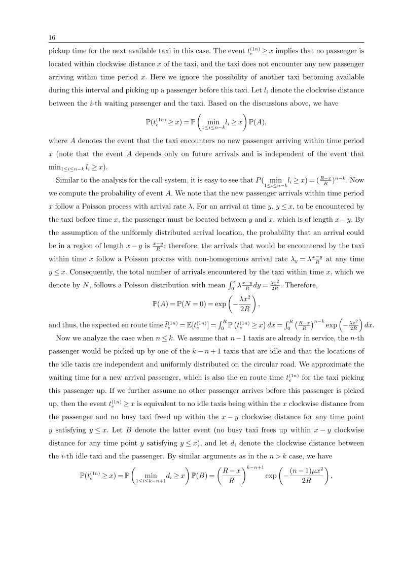
16

pickup time for the next available taxi in this case. The event t(1n)e ≥ x implies that no passenger is

located within clockwise distance x of the taxi, and the taxi does not encounter any new passenger

arriving within time period x. Here we ignore the possibility of another taxi becoming available

during this interval and picking up a passenger before this taxi. Let li denote the clockwise distance

between the i-th waiting passenger and the taxi. Based on the discussions above, we have

P(t(1n)e ≥ x) = P(

min1≤i≤n−k

li ≥ x)P(A),

where A denotes the event that the taxi encounters no new passenger arriving within time period

x (note that the event A depends only on future arrivals and is independent of the event that

min1≤i≤n−k li ≥ x).

Similar to the analysis for the call system, it is easy to see that P ( min1≤i≤n−k

li ≥ x) = (R−xR

)n−k. Now

we compute the probability of event A. We note that the new passenger arrivals within time period

x follow a Poisson process with arrival rate λ. For an arrival at time y, y≤ x, to be encountered by

the taxi before time x, the passenger must be located between y and x, which is of length x−y. By

the assumption of the uniformly distributed arrival location, the probability that an arrival could

be in a region of length x− y is x−yR

; therefore, the arrivals that would be encountered by the taxi

within time x follow a Poisson process with non-homogenous arrival rate λy = λx−yR

at any time

y≤ x. Consequently, the total number of arrivals encountered by the taxi within time x, which we

denote by N , follows a Poisson distribution with mean∫ x0λx−y

Rdy= λx2

2R. Therefore,

P(A) = P(N = 0) = exp

(−λx

2

2R

),

and thus, the expected en route time t(1n)e =E[t(1n)e ] =∫ R0P(t(1n)e ≥ x

)dx=

∫ R0

(R−xR

)n−kexp

(−λx2

2R

)dx.

Now we analyze the case when n≤ k. We assume that n−1 taxis are already in service, the n-th

passenger would be picked up by one of the k−n+ 1 taxis that are idle and that the locations of

the idle taxis are independent and uniformly distributed on the circular road. We approximate the

waiting time for a new arrival passenger, which is also the en route time t(1n)e for the taxi picking

this passenger up. If we further assume no other passenger arrives before this passenger is picked

up, then the event t(1n)e ≥ x is equivalent to no idle taxis being within the x clockwise distance from

the passenger and no busy taxi freed up within the x− y clockwise distance for any time point

y satisfying y ≤ x. Let B denote the latter event (no busy taxi frees up within x− y clockwise

distance for any time point y satisfying y ≤ x), and let di denote the clockwise distance between

the i-th idle taxi and the passenger. By similar arguments as in the n> k case, we have

P(t(1n)e ≥ x) = P(

min1≤i≤k−n+1

di ≥ x)P(B) =

(R−xR

)k−n+1

exp

(−(n− 1)µx2

2R

),

17

and t(1n)e =E[t(1n)e ] =∫ R0P(t(1n)e ≥ x)dx=

∫ R0

(R−xR

)k−n+1exp(− (n−1)µx22R

)dx.

Thus, the one-direction no-call system can be approximated by an M/M/k queue with arrival

rate λ(1n)n = λ and state-dependent service rate

µ(1n)n =

n

1/µ+∫R0 (R−x

R )k−n+1

exp

(− (n−1)µx2

2R

)dx, n≤ k,

k

1/µ+∫R0 (R−x

R )n−k

exp(−λx22R

)dx, n > k.

(2)

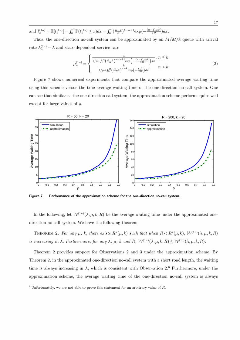
Figure 7 shows numerical experiments that compare the approximated average waiting time

using this scheme versus the true average waiting time of the one-direction no-call system. One

can see that similar as the one-direction call system, the approximation scheme performs quite well

except for large values of ρ.

0 0.1 0.2 0.3 0.4 0.5 0.6 0.7 0.8 0.90

5

10

15

20

25

30

35

40

ρ

Ave

rage

Wai

ting

Tim

e

R = 50, k = 20


0 0.1 0.2 0.3 0.4 0.5 0.6 0.7 0.8 0.90

20

40

60

80

100

120

140

160

ρ

Ave

rage

Wai

ting

Tim

e

R = 200, k = 20


Figure 7 Performance of the approximation scheme for the one-direction no-call system.

In the following, let W(1n)(λ,µ, k,R) be the average waiting time under the approximated one-

direction no-call system. We have the following theorem:

Theorem 2. For any µ, k, there exists R∗(µ,k) such that when R<R∗(µ,k), W(1n)(λ,µ, k,R)

is increasing in λ. Furthermore, for any λ, µ, k and R, W(1n)(λ,µ, k,R)≤W(1c)(λ,µ, k,R).

Theorem 2 provides support for Observations 2 and 3 under the approximation scheme. By

Theorem 2, in the approximated one-direction no-call system with a short road length, the waiting

time is always increasing in λ, which is consistent with Observation 2.6 Furthermore, under the

approximation scheme, the average waiting time of the one-direction no-call system is always

6 Unfortunately, we are not able to prove this statement for an arbitrary value of R.

18

smaller than that of the one-direction call system, which verifies Observation 3. Thus, by using the

approximation scheme, we are able to provide justifications for most of the observations about the

one-direction system.

5. Two-Direction Call/No-Call Systems

In this section, we study the two-direction call/no-call systems. As in Section 4, we first perform

numerical experiments on the systems and summarize our observations. Then, we use an approxi-

mation scheme to obtain theoretical analysis.

5.1. Numerical Experiments

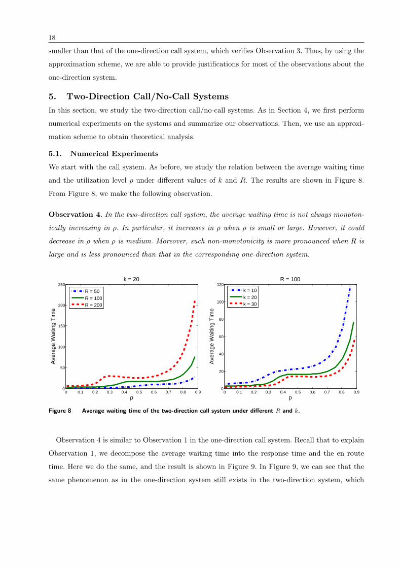
We start with the call system. As before, we study the relation between the average waiting time

and the utilization level ρ under different values of k and R. The results are shown in Figure 8.

From Figure 8, we make the following observation.

Observation 4. In the two-direction call system, the average waiting time is not always monoton-

ically increasing in ρ. In particular, it increases in ρ when ρ is small or large. However, it could

decrease in ρ when ρ is medium. Moreover, such non-monotonicity is more pronounced when R is

large and is less pronounced than that in the corresponding one-direction system.

0 0.1 0.2 0.3 0.4 0.5 0.6 0.7 0.8 0.90

50

100

150

200

250

ρ

Ave

rage

Wai

ting

Tim

e

k = 20

R = 50R = 100R = 200

0 0.1 0.2 0.3 0.4 0.5 0.6 0.7 0.8 0.90

20

40

60

80

100

120

ρ

Ave

rage

Wai

ting

Tim

e

R = 100

k = 10k = 20k = 30

Figure 8 Average waiting time of the two-direction call system under different R and k.

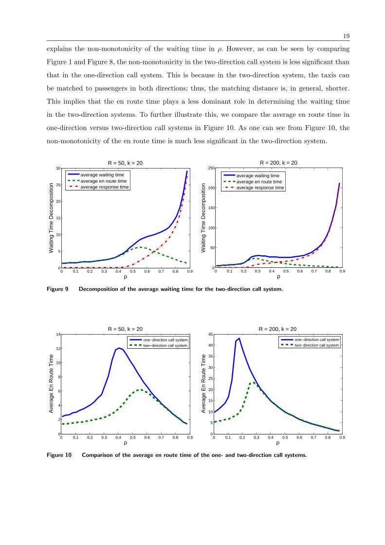
Observation 4 is similar to Observation 1 in the one-direction call system. Recall that to explain

Observation 1, we decompose the average waiting time into the response time and the en route

time. Here we do the same, and the result is shown in Figure 9. In Figure 9, we can see that the

same phenomenon as in the one-direction system still exists in the two-direction system, which

19

explains the non-monotonicity of the waiting time in ρ. However, as can be seen by comparing

Figure 1 and Figure 8, the non-monotonicity in the two-direction call system is less significant than

that in the one-direction call system. This is because in the two-direction system, the taxis can

be matched to passengers in both directions; thus, the matching distance is, in general, shorter.

This implies that the en route time plays a less dominant role in determining the waiting time

in the two-direction systems. To further illustrate this, we compare the average en route time in

one-direction versus two-direction call systems in Figure 10. As one can see from Figure 10, the

non-monotonicity of the en route time is much less significant in the two-direction system.

0 0.1 0.2 0.3 0.4 0.5 0.6 0.7 0.8 0.90

5

10

15

20

25

30

ρ

Wai

ting

Tim

e D

ecom

posi

tion

R = 50, k = 20


0 0.1 0.2 0.3 0.4 0.5 0.6 0.7 0.8 0.90

50

100

150

200

250

ρ

Wai

ting

Tim

e D

ecom

posi

tion

R = 200, k = 20


Figure 9 Decomposition of the average waiting time for the two-direction call system.

0 0.1 0.2 0.3 0.4 0.5 0.6 0.7 0.8 0.90

2

4

6

8

10

12

14

ρ

Ave

rage

En

Rou

te T

ime

R = 50, k = 20

one−direction call systemtwo−direction call system

0 0.1 0.2 0.3 0.4 0.5 0.6 0.7 0.8 0.90

5

10

15

20

25

30

35

40

45

ρ

Ave

rage

En

Rou

te T

ime

R = 200, k = 20

one−direction call systemtwo−direction call system

Figure 10 Comparison of the average en route time of the one- and two-direction call systems.

20

For the two-direction no-call system, we have exactly the same result as in the one-direction

system, which we summarize in the following observation.

Observation 5. The average waiting time in the two-direction no-call system is monotonically

increasing in ρ.

5.2. Approximation Scheme

In this section, we construct an approximation scheme for the two-direction systems. Using the

approximation scheme, we provide justifications for Observations 4 and 5 and show parallel results

as in Theorems 1 and 2.

We apply the idea introduced in Section 4.2, that is, to approximate the system by an M/M/k

queue. In particular, for the two-direction no-call system, since the matching mechanism is exactly

the same as in the one-direction no-call system (except that taxis now are allowed to travel in both

directions), the adopted approximation scheme for the two-direction no-call system is identical to

that of the one-direction no-call system. That is, the approximation scheme for the two-direction

no-call system is an M/M/k queue with arrival rate λ and state-dependent service rates as in (2),

i.e., µ(2n)n = µ(1n)

n . And we have the following theorem:

Theorem 3. Let W(2n)(λ,µ, k,R) be the average waiting time in the approximated two-direction

no-call system. For any µ, k, there exists R(µ,k) such that when R<R(µ,k), W(2n)(λ,µ, k,R) is

increasing in λ.

For the two-direction call system, we use the similar idea as in the one-direction call system.

However, when computing the average en route time t(2c)e , we should consider the distance for

both directions. More specifically, let t(2c)e be the en route time and di be the distance (in the

two-direction sense) between the i-th taxi and a passenger in the two-direction call system. Then,

when n< k, we have

P(t(2c)e ≥ x) =k−n+1∏i=1

P(di ≥ x) =

(R− 2x

R

)k−n+1

and t(2c)e =E[t(2c)e ] =

∫ R/2

0

P(t(2c)e ≥ x)dx=R

2(k−n+ 2).

Similarly, when n> k, we approximate the average en route time t(2c)e by R2(n−k+1)

and when n= k,

we approximate the average en route time by R/4 (which is the average distance between two

uniformly random points on the circle, where the distance is in the two-direction sense). Therefore,

we can approximate the two-direction call system by an M/M/k queue with state-dependent arrival

rate λ(2c)n = λ and service rate

µ(2c)n =

n

1/µ+ R2(k−n+2)

, if n≤ k,k

1/µ+ R2(n−k+1)

, if n> k.(3)

21

We have the following theorem for the approximated two-direction call system:

Theorem 4. Consider the approximated two-direction call system given by (3). Let

W(2c)(λ,µ, k,R) be the average waiting time given parameters λ, µ, k and R. Then we have:

1. W(2c)(λ,µ, k,R)<∞ if and only if 0≤ λ< kµ.

2. For any given µ, k and R, ∂W(2c)(λ,µ,k,R)

∂λ

∣∣∣λ=0≥ 0 and limλ→kµ−

∂W(2c)(λ,µ,k,R)

∂λ> 0.

3. For any given µ and k≥ 2, there exists a constant R∗(µ,k) such that when R>R∗(µ,k), there

exists 0≤ λ(µ,k,R)<kµ such that ∂W(2c)(λ,µ,k,R)

∂λ

∣∣∣λ=λ(µ,k,R)

< 0.

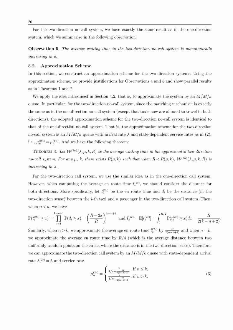
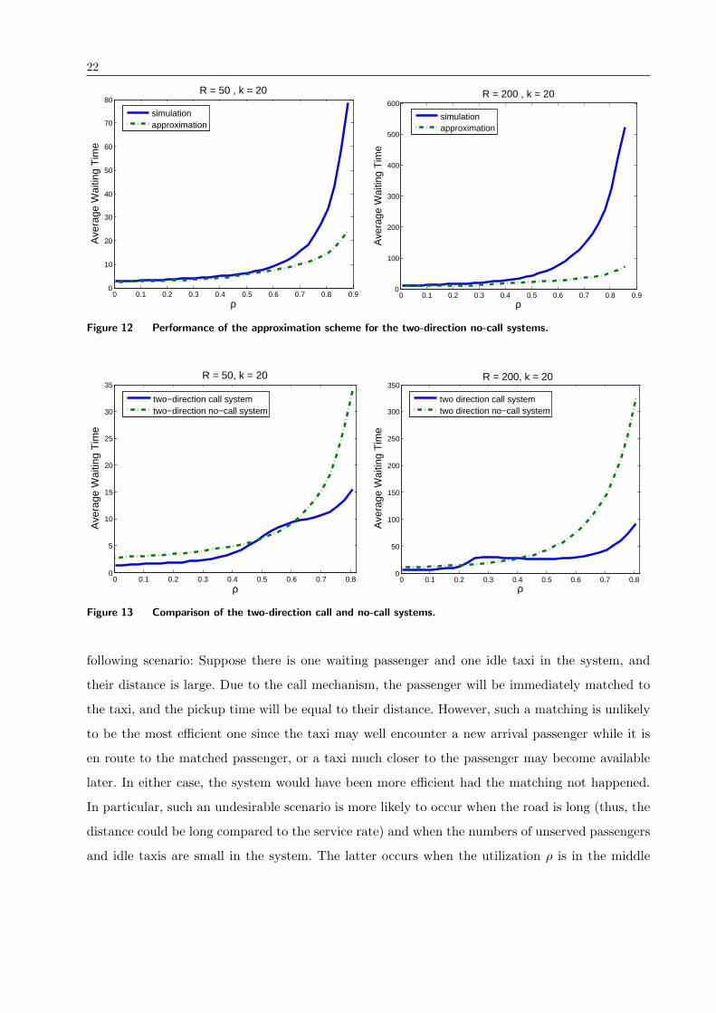
Figures 11 and 12 show comparisons between the approximated systems and the actual systems

in the two-direction case. As one can see from Figures 11 and 12, the approximation scheme is also

quite accurate in the two-direction systems, especially for small and medium values of ρ.

0 0.1 0.2 0.3 0.4 0.5 0.6 0.7 0.8 0.90

5

10

15

20

25

30

ρ

Ave

rage

Wai

ting

Tim

e

R = 50 , k = 20


0 0.1 0.2 0.3 0.4 0.5 0.6 0.7 0.8 0.90

50

100

150

200

250

ρ

Ave

rage

Wai

ting

Tim

eR = 200 , k = 20


Figure 11 Performance of the approximation scheme for the two-direction call systems.

5.3. Comparison between Two-Direction Call and No-Call Systems

In this section, we compare the waiting time in the two-direction call system with that in the

two-direction no-call system. We first obtain some numerical results in Figure 13. As shown in

Figure 13, the average waiting time in the two-direction call system could be larger than that in

the two-direction no-call system when the utilization level ρ is medium, especially when R is large.

Otherwise, the average waiting time in the two-direction call system is smaller than that in the

two-direction no-call system.

To understand this result, we pinpoint the disadvantage of both systems and study when these

disadvantages are most significant. For the call system, its disadvantage can be illustrated by the

22

0 0.1 0.2 0.3 0.4 0.5 0.6 0.7 0.8 0.90

10

20

30

40

50

60

70

80

ρ

Ave

rage

Wai

ting

Tim

eR = 50 , k = 20


0 0.1 0.2 0.3 0.4 0.5 0.6 0.7 0.8 0.90

100

200

300

400

500

600

ρ

Ave

rage

Wai

ting

Tim

e

R = 200 , k = 20


Figure 12 Performance of the approximation scheme for the two-direction no-call systems.

0 0.1 0.2 0.3 0.4 0.5 0.6 0.7 0.80

5

10

15

20

25

30

35

ρ

Ave

rage

Wai

ting

Tim

e

R = 50, k = 20

two−direction call systemtwo−direction no−call system

0 0.1 0.2 0.3 0.4 0.5 0.6 0.7 0.80

50

100

150

200

250

300

350

ρ

Ave

rage

Wai

ting

Tim

eR = 200, k = 20

two direction call systemtwo direction no−call system

Figure 13 Comparison of the two-direction call and no-call systems.

following scenario: Suppose there is one waiting passenger and one idle taxi in the system, and

their distance is large. Due to the call mechanism, the passenger will be immediately matched to

the taxi, and the pickup time will be equal to their distance. However, such a matching is unlikely

to be the most efficient one since the taxi may well encounter a new arrival passenger while it is

en route to the matched passenger, or a taxi much closer to the passenger may become available

later. In either case, the system would have been more efficient had the matching not happened.

In particular, such an undesirable scenario is more likely to occur when the road is long (thus, the

distance could be long compared to the service rate) and when the numbers of unserved passengers

and idle taxis are small in the system. The latter occurs when the utilization ρ is in the middle

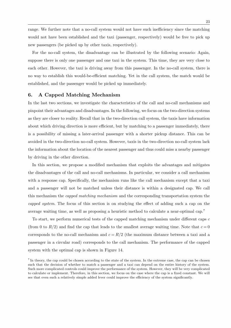
23

range. We further note that a no-call system would not have such inefficiency since the matching

would not have been established and the taxi (passenger, respectively) would be free to pick up

new passengers (be picked up by other taxis, respectively).

For the no-call system, the disadvantage can be illustrated by the following scenario: Again,

suppose there is only one passenger and one taxi in the system. This time, they are very close to

each other. However, the taxi is driving away from this passenger. In the no-call system, there is

no way to establish this would-be-efficient matching. Yet in the call system, the match would be

established, and the passenger would be picked up immediately.

6. A Capped Matching Mechanism

In the last two sections, we investigate the characteristics of the call and no-call mechanisms and

pinpoint their advantages and disadvantages. In the following, we focus on the two-direction systems

as they are closer to reality. Recall that in the two-direction call system, the taxis have information

about which driving direction is more efficient, but by matching to a passenger immediately, there

is a possibility of missing a later-arrival passenger with a shorter pickup distance. This can be

avoided in the two-direction no-call system. However, taxis in the two-direction no-call system lack

the information about the location of the nearest passenger and thus could miss a nearby passenger

by driving in the other direction.

In this section, we propose a modified mechanism that exploits the advantages and mitigates

the disadvantages of the call and no-call mechanisms. In particular, we consider a call mechanism

with a response cap. Specifically, the mechanism runs like the call mechanism except that a taxi

and a passenger will not be matched unless their distance is within a designated cap. We call

this mechanism the capped matching mechanism and the corresponding transportation system the

capped system. The focus of this section is on studying the effect of adding such a cap on the

average waiting time, as well as proposing a heuristic method to calculate a near-optimal cap.7

To start, we perform numerical tests of the capped matching mechanism under different caps c

(from 0 to R/2) and find the cap that leads to the smallest average waiting time. Note that c= 0

corresponds to the no-call mechanism and c=R/2 (the maximum distance between a taxi and a

passenger in a circular road) corresponds to the call mechanism. The performance of the capped

system with the optimal cap is shown in Figure 14.

7 In theory, the cap could be chosen according to the state of the system. In the extreme case, the cap can be chosensuch that the decision of whether to match a passenger and a taxi can depend on the entire history of the system.Such more complicated controls could improve the performance of the system. However, they will be very complicatedto calculate or implement. Therefore, in this section, we focus on the case where the cap is a fixed constant. We willsee that even such a relatively simple added lever could improve the efficiency of the system significantly.

24

0 0.1 0.2 0.3 0.4 0.5 0.6 0.7 0.8 0.90

50

100

150

200

250

300

350

ρ

Ave

rage

Wai

ting

Tim

eR = 100 , k = 10

optimal capped systemcall systemno−call system

0 0.1 0.2 0.3 0.4 0.5 0.6 0.7 0.8 0.90

50

100

150

ρ

Ave

rage

Wai

ting

Tim

e

R = 100 , k = 20


0 0.1 0.2 0.3 0.4 0.5 0.6 0.7 0.8 0.90

20

40

60

80

100

120

ρ

Ave

rage

Wai

ting

Tim

e

R = 100 , k = 30


Figure 14 Comparison of the two-direction optimal capped system, no-call system and call system.

From Figure 14, we can see that the capped system with the optimal cap outperforms the call

and no-call systems under different parameter settings. In particular, using an optimal cap could

significantly reduce the average waiting time, and the reduction is more significant when there are

more taxis in the system.

Having observed the potential value of adding a cap, a natural question is how to obtain a good

cap without having to go through extensive simulations. In the following, we propose a heuristic

method that provides a cap with good performance.

To find a good cap such that we should match a taxi and a passenger if their distance is within

the cap and should not otherwise, we consider the following question: How close do a taxi and a

passenger need to be so that matching them would be a good matching? To answer this question,

we think from the taxi’s point of view. Recall that if we establish a match between a taxi and a

passenger, then the en route time for this taxi will be equal to the distance between the taxi and

the passenger. Now we approximate the expected time this taxi has to drive in order to encounter

a passenger if we do not establish the match. If the expected time is shorter than the distance from

the current passenger, then intuitively the current match is not efficient, in which case we should

not match them. Otherwise, matching will result in a shorter en route time than not matching, in

which case we should match them.

Now it remains to calculate the expected time the taxi has to drive in order to encounter a

passenger. To this end, we first compute the probability that a new passenger arrival will be

encountered by this taxi within time x. Remember that new passengers arrive according to a

Poisson process with rate λ. Similar to the discussions in Section 4.2, for an arrival at time y, y≤ x,

to be encountered by the taxi before time x, the passenger must be located between y and x, which

is of length x−y. By the assumption of the uniformly distributed arriving location, the probability

that an arrival will be in a region of length x − y is x−yR

; therefore, the arrivals that would be

encountered by the taxi within time x follow a Poisson process with a non-homogenous arrival rate

25

λy = λx−yR

at any time y ≤ x. Consequently, the total number of arrivals encountered by the taxi

within time x, which we denote by N , follows a Poisson distribution with mean∫ x0λx−y

Rdy = λx2

2R.

Therefore, the probability that it takes longer than x for a taxi to encounter a passenger equals

P(N = 0) = exp

(−λx

2

2R

),

and the expected time for a taxi to encounter a passenger is∫ ∞0

exp

(−λx

2

2R

)dx=

√πR

2λ.

Thus, based on the above idea, we choose a heuristic cap c∗ to be c∗ = min{R/2,

√πR2λ

}. Here, we

add the term R/2 because for any c∗ ≥R/2, the mechanism will be equivalent to a call mechanism.

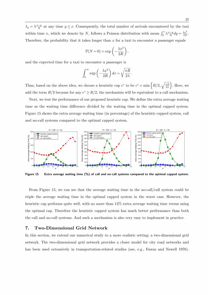
Next, we test the performance of our proposed heuristic cap. We define the extra average waiting

time as the waiting time difference divided by the waiting time in the optimal capped system.

Figure 15 shows the extra average waiting time (in percentage) of the heuristic capped system, call

and no-call systems compared to the optimal capped system.

0 0.1 0.2 0.3 0.4 0.5 0.6 0.7 0.8 0.9 0%

50%

100%

150%

200%

250%

ρ

Ext

ra A

vera

ge W

aitin

g T

ime

(%)

R = 100 , k = 10

heuristic capped systemcall systemno−call system

0 0.1 0.2 0.3 0.4 0.5 0.6 0.7 0.8 0.9 0%

20%

40%

60%

80%

100%

120%

140%

160%

180%

200%

ρ

Ext

ra A

vera

ge W

aitin

g T

ime

(%)

R = 100 , k = 20


0 0.1 0.2 0.3 0.4 0.5 0.6 0.7 0.8 0.9 0%

20%

40%

60%

80%

100%

120%

140%

160%

180%

200%

ρ

Ext

ra A

vera

ge W

aitin

g T

ime

(%)

R = 100 , k = 30


Figure 15 Extra average waiting time (%) of call and no-call systems compared to the optimal capped system.

From Figure 15, we can see that the average waiting time in the no-call/call system could be

triple the average waiting time in the optimal capped system in the worst case. However, the

heuristic cap performs quite well, with no more than 12% extra average waiting time versus using

the optimal cap. Therefore the heuristic capped system has much better performance than both

the call and no-call systems. And such a mechanism is also very easy to implement in practice.

7. Two-Dimensional Grid Network

In this section, we extend our numerical study to a more realistic setting: a two-dimensional grid

network. The two-dimensional grid network provides a closer model for city road networks and

has been used extensively in transportation-related studies (see, e.g., Fawaz and Newell 1976).

26

In particular, we consider a rectangular region that is divided into equally sized sub-squares by

vertical and horizontal roads. The sub-squares may be viewed as blocks in the city. Mathematically,

an m× n two-dimensional grid network is comprised of roads of {x= k,1≤ y ≤ n}, k = 1, . . . ,m

and {y= l,1≤ x≤m}, l= 1, . . . , n. In the numerical experiments, we simulate the call and no-call

systems in the two-dimensional grid network to see if the characteristics of these systems in the

circular road setting still hold.

In the simulation, we assume that the passengers’ arrival still follows a Poisson process and they

arrive only at intersection points of the road, i.e., passengers arrive only at points (x, y) where

1 ≤ x ≤m and 1 ≤ y ≤ n are both integers. This is mainly for the simplicity of analysis, yet it

is also plausible in practice. Taxis drive on the road, and at each intersection point, they choose

either to keep the current direction or turn left or right (each option is available only when it

is eligible) in a uniformly random manner. Note that under this setup, a taxi would not drive

back and forth between two adjacent intersection points, which is reasonable and intuitively more

efficient in practice. We assume taxis drive one block per unit of time, and the system is updated

at each integer point of time. In the no-call system, at the end of each time epoch, if an available

taxi encounters a passenger at an intersection, then a match between this taxi and the passenger

will be established immediately. In the call system, at the end of each time epoch, if there are

available taxis in the system, then the passengers who arrive within the past unit of time will be

matched one by one to the taxis in a first-come-first-serve manner. In either system, regardless of

the pickup point, the passenger’s destination is uniformly distributed over all intersection points

in the grid. For the service rate, we first calculate the average distance (1-norm distance) between

any two uniformly random points on the grid and choose µ to be the reciprocal of the average

distance. By simple calculation, we have µ= 3mn/(m(n2− 1) +n(m2− 1)).

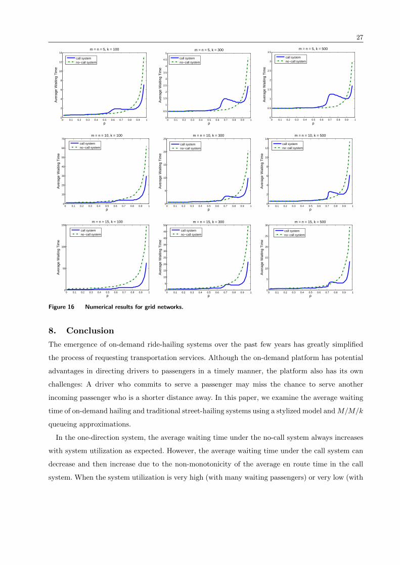
In the following, we perform numerical experiments using grid networks of different sizes and

with different numbers of taxis. As shown in Figure 16, the main features that we have observed in

the circular road setting still hold. In particular, the no-call mechanism could be more efficient than

the call mechanism when the utilization is in the middle range. Otherwise, the call mechanism is

more efficient. Moreover, we observe that in the grid network, the call mechanism tends to be more

efficient when there are few taxis in the system or when the grid is large. This is because if the

grid is large (with many roads in the grid), then the call mechanism would be more advantageous

in helping taxis find passengers. Imagine a network with numerous roads; in that case, it is hard

for a taxi to find a passenger without using a call mechanism. Similarly, when there are very few

taxis, it is hard for them to find passengers without using the call mechanism too. Thus, the call

mechanism is more efficient in those settings.

27

0 0.1 0.2 0.3 0.4 0.5 0.6 0.7 0.8 0.9 10

2

4

6

8

10

12

14

ρ

Ave

rage

Wai

ting

Tim

e

m = n = 5, k = 100


0 0.1 0.2 0.3 0.4 0.5 0.6 0.7 0.8 0.9 10

0.5

1

1.5

2

2.5

3

3.5

4

4.5

5

ρ

Ave

rage

Wai

ting

Tim

e

m = n = 5, k = 300


0 0.1 0.2 0.3 0.4 0.5 0.6 0.7 0.8 0.9 10

0.5

1

1.5

2

2.5

3

3.5

ρ

Ave

rage

Wai

ting

Tim

e

m = n = 5, k = 500


0 0.1 0.2 0.3 0.4 0.5 0.6 0.7 0.8 0.9 10

10

20

30

40

50

60

70

ρ

Ave

rage

Wai

ting

Tim

e

m = n = 10, k = 100


0 0.1 0.2 0.3 0.4 0.5 0.6 0.7 0.8 0.9 10

5

10

15

20

25

ρ

Ave

rage

Wai

ting

Tim

e

m = n = 10, k = 300


0 0.1 0.2 0.3 0.4 0.5 0.6 0.7 0.8 0.9 10

2

4

6

8

10

12

14

ρ

Ave

rage

Wai

ting

Tim

e

m = n = 10, k = 500


0 0.1 0.2 0.3 0.4 0.5 0.6 0.7 0.8 0.9 10

50

100

150

ρ

Ave

rage

Wai

ting

Tim

e

m = n = 15, k = 100


0 0.1 0.2 0.3 0.4 0.5 0.6 0.7 0.8 0.9 10

5

10

15

20

25

30

35

40

45

50

ρ

Ave

rage

Wai

ting

Tim

e

m = n = 15, k = 300


0 0.1 0.2 0.3 0.4 0.5 0.6 0.7 0.8 0.9 10

5

10

15

20

25

30

ρ

Ave

rage

Wai

ting

Tim

e

m = n = 15, k = 500


Figure 16 Numerical results for grid networks.

8. Conclusion

The emergence of on-demand ride-hailing systems over the past few years has greatly simplified

the process of requesting transportation services. Although the on-demand platform has potential

advantages in directing drivers to passengers in a timely manner, the platform also has its own

challenges: A driver who commits to serve a passenger may miss the chance to serve another

incoming passenger who is a shorter distance away. In this paper, we examine the average waiting

time of on-demand hailing and traditional street-hailing systems using a stylized model andM/M/k

queueing approximations.

In the one-direction system, the average waiting time under the no-call system always increases

with system utilization as expected. However, the average waiting time under the call system can

decrease and then increase due to the non-monotonicity of the average en route time in the call

system. When the system utilization is very high (with many waiting passengers) or very low (with

28

many idle drivers), the average en route time is low, whereas the average en route time reaches the

highest when the system utilization is medium, i.e., the system is balanced. In addition, the average

waiting time under the call system is always higher than that in the no-call system. This is because

a call system may have the disadvantage of forgoing possible future matching opportunities when

accepting an incoming request, while a no-call system circumvents it by postponing the “matching”

between a driver and a passenger as late as possible. That is, no matching is established until a

driver is passing a passenger.

In the two-direction system, the average waiting time under a no-call system still increases with

system utilization. In addition, albeit less pronounced, the non-monotonicity of the average waiting

time under a call system is still observed. However, unlike in the one-direction system, a call system

can be better than a no-call system in the two-direction system despite the disadvantage of forgoing

possible future matching opportunities because a call system informs the driver of the shortest

distance to pick up a passenger. It is especially true when the system utilization is either very low

or very high. When the system utilization is medium, a no-call system may still perform better

than a call system in reducing the average waiting time.

Based on the understanding of the two different matching mechanisms in one and two directions,

we sought to address the matching inefficiency that arises with the on-demand hailing platform

by proposing a distance cap in responding to requests from passengers. The distance cap, on one

hand, reserves the advantages of the on-demand hailing system, while on the other hand helps in

limiting the possibility of serving an incoming passenger. We propose a heuristic way to calculate

the distance cap that is not only implementable but also effectively reduces average waiting time in

the on-demand hailing system. In a more complex grid network, we show that properties observed

in the circular road system still exist. A no-call system may perform better than a call system

when there are more taxis or when the network is less complicated.

In sum, our analysis shows that the on-demand hailing system is more efficient than the tra-

ditional street-hailing system in some circumstances while it is less efficient in others. Awareness

of advantages and disadvantages of the on-demand hailing system and street hailing would assist

policy makers decide when and where to adopt on-demand hailing or street hailing. In particular,

we show that street hailing may have its own value in operations and should be reserved under

certain conditions. This research may provide justification for the New York City government to

allow a certain number of taxis dedicated to street hailing through Street Hail Livery (SHL), and

evidence that it may not be unreasonable for the Shanghai government to ban on-demand hailing

apps during certain times of the day from an operations aspect. Our paper provides guidance for

29

evaluating the efficiency of each system. In addition, to take advantage of both systems, we propose

a simple yet effective solution: using a distance cap to avoid the inefficiency in matching through an

on-demand platform, and thus significantly reduce the average waiting time. Our work will inspire

a few interesting future research directions, such as the accuracy of the approximation scheme,

the extension of the theoretical results to more complex road networks, and the validation of our

findings using real data.

References

Akbarpour, M., S. Li, O. G. Shayan. 2016. Thickness and information in dynamic matching markets. Working

Paper.

Allon, G., A. Bassamboo, E. B. Cil. 2012. Large-scale service marketplaces: The role of the moderating firm.

Management Science 58(10) 1854–1872.

Anderson, R., I. Ashlagi, D. Gamarnik, Y. Kanoria. 2015. A dynamic model of barter exchange. In SODA’15:

Proceedings of the 26th Annual ACM-SIAM Symposium on Discrete Algorithms. 1925–1933.

Baccara, M., S. Lee, L. Yariv. 2015. Optimal dynamic matching. Working Paper.

Bailey, W., T. Clark. 1992. Taxi management and route control: A systems study and simulation experiment.

Proceedings of the 24th Conference on Winter Simulation. 1217–1222.

Benjaafar, S., G. Kong, X. Li, C. Courcoubetis. 2015. Peer-to-peer product sharing: Implications for owner-

ship, usage and social welfare in the sharing economy. Working Paper.

Cachon, G. P., K. M. Daniels, R. Lobel. 2015. The role of surge pricing on a service platform with self-

scheduling capacity. Working Paper.

Cullen, Z., C. Farronato. 2014. Outsourcing tasks online: Matching supply and demand on peer-to-peer

internet platforms. Working Paper.

Fawaz, M. Y., G. F. Newell. 1976. Optimal spacings for a rectangular grid transportation network: A

hierarchy structure. Transportation Research 10(2) 111–119.

Fraiberger, S. P., A. Sundararajan. 2015. Peer-to-peer rental markets in the sharing economy. Working

Paper.

Gurvich, I., M. Lariviere, A. Moreno. 2015. Operations in the on-demand economy: Staffing services with

self-scheduling capacity. Working Paper.

Hawkins, A. J. 2016a. It took Uber five years to get to a billion rides, and its Chinese rival just did it in

one. The Verge .

Hawkins, A. J. 2016b. Uber just completed its two-billionth trip @Verge. http://www.theverge.com/2016/

7/18/12211710/uber-two-billion-trip-announced-kalanick-china-didi. Accessed: 2017-04-21.

Hu, M., Y. Zhou. 2016. Dynamic type matching. Working Paper.

30

Jiang, B., L. Tian. 2016. Collaborative consumption: Strategic and economic implications of product sharing.

Management Science. Forthcoming.

McLeod, M. G. 1972. The operation and performance of a taxi fleet. Master’s thesis, Massachusetts Institute

of Technology.

Meyer, R., H. Wolfe. 1961. The organization and operation of a taxi fleet. Naval Research Logistics Quarterly

8(2) 137–150.

Riquelme, C., S. Banerjee, R. Johari. 2015. Pricing in ride-share platforms: A queueing-theoretic approach.

Working Paper.

Rogers, B. 2015. The social costs of Uber. University of Chicago Law Review Dialogue 82.

Steinberg, J. 2012. Smartphone taxi e-hail apps: New convenience or potential deathtrap. The Forbes .

Tang, C. S., J. Bai, K. C. So, X. Chen, H. Wang. 2016. Coordinating supply and demand on an on-demand

platform: Price, wage, and payout ratio. Working Paper.

Taylor, T. 2016. On-demand service platforms. Working Paper.

Welch, P. 1983. The statistical analysis of simulation results. The Computer Performance Modeling Hand-

book . Academic Press, 268–328.

Wood, D. 1992. The Computation of Polylogarithms. University of Kent at Canterbury.

ONLINE APPENDIX

Lemma 1. Consider an M/M/k queue with arrival rate λ and state-dependent service rate

µn =

{n(k−n+2)

R, if n≤ k,

k(n−k+1)

R, if n> k.

Let W(λ,k,R) be the average waiting time. Then for any R> 0 and k ≥ 2, there exists an arrival

rate λ∗(k,R) such that ∂W(λ,k,R)

∂λ

∣∣∣λ=λ∗(k,R)

< 0.

Proof of Lemma 1. By standard queueing theory,W(λ,k,R) =∑∞i=1

iλi−1

µ1µ2···µi1+∑∞i=1

λiµ1µ2···µi

. For∑∞

i=1λi

µ1µ2···µi,

we have∑∞

i=1λi

µ1µ2···µi=∑k−1

i=1λi

µ1µ2···µi+∑∞

i=kλi

µ1µ2···µi, where

∞∑i=k

λi

µ1µ2 · · ·µi=

λk

µ1µ2 · · ·µk

(1 +

∞∑i=k+1

λi−k

µk+1 · · ·µi

)

=λk

µ1µ2 · · ·µk

(1 +

∞∑i=k+1

(λR/k)i−k

(i− k+ 1)!

)

=λk

µ1µ2 · · ·µkk

λR

((λR/k) +

∞∑i=k+1

(λR/k)i−k+1

(i− k+ 1)!

)

=λk−1

2µ1µ2 · · ·µk−1

∞∑i=1

(λR/k)i

i!=

λk−1

2µ1µ2 · · ·µk−1(eλR/k− 1).

Similarly, for∑∞

i=1 iλi−1

µ1µ2···µi, we have

∑∞i=1 i

λi−1

µ1µ2···µi=∑k−1

i=1 iλi−1

µ1µ2···µi+∑∞

i=k iλi−1

µ1µ2···µi, where

∞∑i=k

iλi−1

µ1µ2 · · ·µi=

λk−1

µ1µ2 · · ·µk

(k+

∞∑i=k+1

iλi−k

µk+1 · · ·µi

)

=λk−1

µ1µ2 · · ·µkk

λR

(kλR

k+

∞∑i=k+1

i(λR/k)i−k+1

(i− k+ 1)!

)

=λk−2

2µ1µ2 · · ·µk−1

∞∑i=k

i(λR/k)i−k+1

(i− k+ 1)!

=λk−2

2µ1µ2 · · ·µk−1

((k− 1)

∞∑i=k

(λR/k)i−k+1

(i− k+ 1)!+∞∑j=1

j(λR/k)j

j!

)=

λk−2

2µ1µ2 · · ·µk−1

[(k− 1)(eλR/k− 1) +

λR

keλR/k

].

Therefore

W(λ,k,R) =

∑k−1i=1 i

λi−1

µ1µ2···µi+ λk−2

2µ1µ2···µk−1[(k− 1)(eλR/k− 1) + λR

keλR/k]

1 +∑k−1

i=1λi


2µ1µ2···µk−1(eλR/k− 1)

.

For any given R and k ≥ 2, we note that W∣∣λ=0

= R/(k + 1) and W∣∣λ→∞ = R/k. Also we claim

that for any given R and k ≥ 2, there exists λ such that W∣∣λ=λ

>R/k. To see this, when k = 2,

1

2

we can simplify the expression of W and get that W = 1+(1+λR/2) exp (λR/2)

λ+6/R+λ exp (λR/2). By taking λ satisfying

exp (λR/2)> 2 + λR/2, we have W∣∣λ=λ

>R/2. When k > 2, we have

W >

λk−2

2µ1µ2···µk−1[(k− 1)(eλR/k− 1) + λR

keλR/k]

1 +∑k−1

i=1λi


2µ1µ2···µk−1(eλR/k− 1)

>

λk−1

2µ1µ2···µk−1(k− 1 + eλR/k)R

k

1 +∑k−1

i=1λi


2µ1µ2···µk−1(eλR/k− 1)

.

Taking λ satisfying kλk−1

2µ1µ2···µk−1> 1 +

∑k−1i=1

λi

µ1µ2···µi(note such λ must exist since the left-hand side

is greater than the right-hand side when λ is large), we obtain W∣∣λ=λ

>R/k.

Thus for any given R and k ≥ 2, W∣∣λ=0

=R/(k+ 1) and W∣∣λ→∞ =R/k, and there exists λ such

that W∣∣λ=λ

> R/k. Also it is easy to see that W is continuously differentiable in λ on λ > 0.

Therefore there exists λ∗(k,R) such that ∂W(λ,k,R)

∂λ

∣∣∣λ=λ∗(k,R)

< 0. �

Lemma 2. For any given R> 0 and k≥ 2, there exist constants λ∗(k,R) and µ∗(λ∗(k,R), k,R)

such that ∂W(λ,µ,k,R)

∂λ

∣∣∣λ=λ∗(k,R)

< 0 for any µ > µ∗(λ∗(k,R), k,R), where W(λ,µ, k,R) =∑∞i=1

iλi−1

µ1µ2···µi1+∑∞i=1

λiµ1µ2···µi

− 1/µ, with µi = µ(1c)i as defined in (??).

Proof of Lemma 2. Take derivative of W(λ,µ, k,R) with respect to λ, we have that

∂W(λ,µ, k,R)

∂λ=

∑∞i=2

i(i−1)λi−2

µ1µ2···µi(1 +

∑∞i=1

λi

µ1µ2···µi)− (

∑∞i=1

iλi−1

µ1µ2···µi)2

(1 +∑∞

i=1λi

µ1µ2···µi)2

.

Let ai(µ) = λi

µ1µ2···µi, bi(µ) = iλi−1

µ1µ2···µiand ci(µ) = i(i−1)λi−2

µ1µ2···µi. We first show that for any µ,k,R and

0≤ λ< kµ,∑∞

i=1 ai(µ),∑∞

i=1 bi(µ) and∑∞

i=2 ci(µ) are all finite. To do so, define ε= 12(k/λ−1/µ)>

0 and N = min{i : 0≤ R(i−k+1)

≤ ε}. We have

∞∑i=1

ai(µ) =N∑i=1

λi

µ1µ2 · · ·µi+

λN

µ1µ2 · · ·µN

∞∑i=1

λi

µN+1µN+2 · · ·µN+i

<N∑i=1

λi

µ1µ2 · · ·µi+

λN

µ1µ2 · · ·µN

∞∑i=1

λi(1/µ+ ε)i

ki

<N∑i=1

λi

µ1µ2 · · ·µi+

λN

µ1µ2 · · ·µNkµ+λ

kµ−λ<∞,

where the first inequality is because µl >k

1/µ+εfor any l ≥ N + 1. Similarly, we can also prove∑∞

i=1 bi <∞, and∑∞

i=2 ci <∞ when 0≤ λ< kµ.

With the finiteness of∑∞

i=1 ai,∑∞

i=1 bi and∑∞

i=2 ci,∂W(λ,µ,k,R)

∂λis finite as well. We also note that

ai(µ), bi(µ) and ci(µ) are all continuous and decreasing in µ. Therefore by the monotone convergence

theorem,

limµ→∞

∞∑i=1

ai(µ) =∞∑i=1

limµ→∞

ai(µ), limµ→∞

∞∑i=1

bi(µ) =∞∑i=1

limµ→∞

bi(µ), and limµ→∞

∞∑i=2

ci(µ) =∞∑i=2

limµ→∞

ci(µ).

3

We thus have that for any given k,R and 0≤ λ< kµ,

limµ→∞

∂W∂λ

=limµ→∞

∑∞i=2

i(i−1)λi−2

µ1µ2···µi(1 + limµ→∞

∑∞i=1

λi

µ1µ2···µi)− limµ→∞(

∑∞i=1

iλi−1

µ1µ2···µi)2

limµ→∞(1 +∑∞

i=1λi

µ1µ2···µi)2

(1)

=

∑∞i=2

i(i−1)λi−2

limµ→∞(µ1µ2···µi)(1 +

∑∞i=1

λi

limµ→∞(µ1µ2···µi))− (

∑∞i=1

iλi−1

limµ→∞(µ1µ2···µi))2

(1 +∑∞

i=1λi

limµ→∞(µ1µ2···µi))2

=∂W∂λ

, (2)

where W is defined in Lemma 1. Here the first equation holds since all limits exist and are finite,

and the limit for the denominator is not zero.

By Lemma 1, for any given R and k, there exists λ∗(k,R) such that ∂W∂λ

∣∣∣λ=λ∗(k,R)

< 0. Thus, by

(2), there exists µ∗ such that when µ>µ∗, ∂W∂λ

∣∣λ=λ∗(k,R)

< 0. Thus the lemma is proved. �

Proof of Theorem 1. In the following, we will prove the three parts of Theorem 1 separately.

For the ease of notation, we omit the superscripts in µis, λis and W(·) as the meanings are clear

from the context.

Part 1. For the approximated one-direction call system, the expected waiting time W(λ,µ, k,R)

satisfies that W =∑∞i=1

iλi−1

µ1µ2···µi1+∑∞i=1

λiµ1µ2···µi

−1/µ, where µis are defined in (??). When λ≥ kµ, since µi ≤ kµ

for all i, it is easy to see that W(λ,µ, k,R) =∞. Therefore it remains to prove that when λ< kµ,

W(λ,µ, k,R) <∞. It is equivalent to show∑∞

i=1iλi−1

µ1µ2···µiand

∑∞i=1

λi

µ1µ2···µiare both finite when

0≤ λ < kµ. Note that in the proof of Lemma 2 we have proved the finiteness of these two terms.

Therefore, W(λ,µ, k,R)<∞ if and only if 0≤ λ< kµ and thus the first part is proved.

Part 2. We first show that ∂W∂λ

∣∣λ=0≥ 0. To see that, we take derivative of W with respect to λ,

we have

∂W∂λ

=

∑∞i=2

i(i−1)λi−2

µ1µ2···µi(1 +

∑∞i=1

λi

µ1µ2···µi)− (

∑∞i=1

iλi−1

µ1µ2···µi)2

(1 +∑∞

i=1λi

µ1µ2···µi)2

.

We have that

∂W∂λ

∣∣∣∣λ=0

=2

µ1µ2

− 1

µ21

=

1µ1

( 1µ

+ R2

), if k= 1,R6µ1, if k= 2,

1µ1

(Rk− R

k+1), if k > 2.

Therefore, ∂W∂λ

∣∣λ=0≥ 0.

Next, we prove that limλ→kµ−∂W(λ,µ,k,R)

∂λ> 0. It suffices to show that

limλ→kµ−

∞∑i=2

i(i− 1)λi−2

µ1µ2 · · ·µi

(1 +

∞∑i=1

λi

µ1µ2 · · ·µi

)−

(∞∑i=1

iλi−1

µ1µ2 · · ·µi

)2> 0. (3)

Let 0 < ε < 1 be a constant such that (1 − ε)2(µR + 2) − (1 + ε)2(µR + 1) > 12, and M =⌈

max

{µR−k+1µR√

11−ε−1

, k−21− µR√

11+ε

}⌉+ 1. Here we use dxe to denote the smallest integer that is greater

4

than x. In the following, for the ease of notation, we assume µR is an integer. The case when µR is

not an integer can be proved in a very similar way, however, the notation would be much messier.

For i≥ µR+M + 1, by the definition of µn, we have

λi

µ1 · · ·µi=

(λ

kµ

)ikk

k!

k∏`=1

(1 +

µR

k− `+ 2

) i∏`=k+1

(1 +

µR

`− k+ 1

)=C1

(λ

kµ

)i i∏`=M+1

(1 +

µR

`− k+ 1

)where C1 = kk

k!

∏k

`=1(1 + µRk−`+2

)∏M

`=k+1(1 + µR`−k+1

) is a constant. We have

i∏`=M+1

(1 +

µR

`− k+ 1

)=

(µR+M + 2− k)(µR+M + 3− k) · · · (µR+ i+ 1− k)

(M + 2− k)(M + 3− k) · · · (i+ 1− k)

=(i+ 2− k) · · · (i+ 1− k+µR)

(M + 2− k) · · · (M + 1− k+µR)∈

((i+ 1− k+µR

M + 1− k+µR

)µR,

(i+ 2− kM + 2− k

)µR)where in the second equality i≥ µR+M + 1 and µR ∈Z+ are applied. By the definition of M , we

have thati∏

`=M+1

(1 +

µR

`− k+ 1

)∈

{(1− ε)

(i

M

)µR, (1 + ε)

(i

M

)µR}.

Therefore, for i≥ µR+M + 1,

λi

µ1 · · ·µi∈

{C1(1− ε)

(λ

kµ

)i(i

M

)µR,C1(1 + ε)

(λ

kµ

)i(i

M

)µR}.

Similarly, we have

iλi−1

µ1 · · ·µi∈

{C1(1− ε)i

kµ

(λ

kµ

)i−1(i

M

)µR,C1(1 + ε)i

kµ

(λ

kµ

)i−1(i

M

)µR}and

i(i− 1)λi−2

µ1 · · ·µi∈

{C1(1− ε)i(i− 1)

(kµ)2

(λ

kµ

)i−2(i

M

)µR,C1(1 + ε)i(i− 1)

(kµ)2

(λ

kµ

)i−2(i

M

)µR}.

Therefore, we have

∞∑i=1

λi

µ1 · · ·µi=

M∑i=1

λi

µ1 · · ·µi+

∞∑i=M+1

λi

µ1 · · ·µi≥C2 +

C1(1− ε)MµR

∞∑i=1

(λ

kµ

)iiµR

where C2 =−MC1(1− ε)≤∑M

i=1λi

µ1···µi− C1(1−ε)

MµR

∑M

i=1

(λkµ

)iiµR is a constant. Similarly,

∞∑i=2

i(i− 1)λi−2

µ1 · · ·µi≥C ′2 +

C1(1− ε)(kµ)2MµR

∞∑i=2

(λ

kµ

)i−2(i− 1)iµR+1,

where C ′2 =−C1M3(1− ε)/(kµ)2 ≤

∑M

i=2i(i−1)λi−2

µ1···µi− C1(1−ε)

(kµ)2MµR

∑M

i=2(λkµ

)i−2(i− 1)iµR+1 and

∞∑i=1

iλi−1

µ1 · · ·µi≤C ′′2 +

C1(1− ε)kµMµR

∞∑i=1

(λ

kµ

)i−1iµR+1,

5

where C ′′2 =M 2kM ≥∑M

i=1iλi−1

µ1···µi− C1(1−ε)

kµMµR

∑M

i=1(λkµ

)i−1iµR+1.

In the following, we define

f0(p) =∞∑i=1

piiµR, f1(p) =∞∑i=1

pi−1iµR+1 and f2(p) =∞∑i=2

pi−2(i− 1)iµR+1.

Using these functions, the left-hand side of (3) can be written as:∑∞i=2

i(i−1)λi−2

µ1µ2···µi

(1 +

∑∞i=1

λi

µ1µ2···µi

)−(∑∞

i=1iλi−1

µ1µ2···µi

)2

≥(C ′2 + C1(1−ε)

(kµ)2MµR f2

(λkµ

))(C2 + C1(1−ε)

MµR f0

(λkµ

))−(C ′′2 + C1(1+ε)

kµMµR f1

(λkµ

))2

.(4)

In the following, we use the notation of polylogarithm, in which Lis(z) =∑∞

i=1zi

is. Then we have

f0(p) = Li−µR(p), f1(p) =1

pLi−µR−1(p), and f2(p) =

1

p2(Li−µR−2(p)−Li−µR−1(p)).

By the limiting behavior of the polylogarithm (Wood 1992), we have that

limp→1−

f0(p) =Γ(1 +µR)

(−logp)µR+1, lim

p→1−f1(p) =

Γ(2 +µR)

(−logp)µR+2, and lim

p→1−f2(p) =

Γ(3 +µR)

(−logp)µR+3− Γ(2 +µR)

(−logp)µR+2

where Γ(·) is the Gamma function. Therefore,

limp→1−(1− ε)2f0(p)f2(p)− (1 + ε)2f1(p)2

= ((1− ε)2(µR)!(µR+ 2)!− (1 + ε)2(µR+ 1)!2)(−logp)−2µR−4− (1− ε)2(µR)!(µR+ 1)!(−logp)−2µR−3

= (µR)!(µR+ 1)![(1− ε)2(µR+ 2)− (1 + ε)2(µR+ 1)](−logp)−2µR−4− (1− ε)2(µR)!(µR+ 1)!(−logp)−2µR−3

≥ (µR)!(µR+ 1)!

(1

2(−logp)−2µR−4− (1− ε)2(−logp)−2µR−3

)= O(−logp)−2µR−4 > 0

where the inequality is because of the definition of ε. Based on these results, for equation (4), we

further have that

limλ→kµ−

(∑∞i=2

i(i−1)λi−2

µ1µ2···µi

)(1 +

∑∞i=1

λi

µ1µ2···µi

)−(∑∞

i=1iλi−1

µ1µ2···µi

)2

≥ limλ→kµ−

(C ′′2 + C1(1−ε)

(kµ)2MµR f2

(λkµ

))(C2 + C1(1−ε)

MµR f0

(λkµ

))−(C ′2 + C1(1+ε)

kµMµR f1

(λkµ

))2

=O(−log( λkµ

))−2µR−4.

(5)

The last step is because the other terms are smaller in order than O(−log( λkµ

))−2µR−4. Therefore,

limλ→kµ−∂W(λ,µ,k,R)

∂λ> 0. And part 2 is proved.

Part 3. By standard queueing theory,W(λ,µ, k,R) =∑∞i=1

iλi−1

µ1µ2···µi1+∑∞i=1

λiµ1µ2···µi

−1/µ. Now we consider a new

approximated one-direction call system with arrival rate Rλ, service rate Rµ and road length 1.

Note that the new system is equivalent to the original system after scaling the time in the original

system by a factor of 1/R (one unit of time in the original system corresponds to 1/R units of time

6

in the new system). Therefore the corresponding expected waiting time W(Rλ,Rµ,k,1) satisfies

that W(Rλ,Rµ,k,1) = 1RW(λ,µ, k,R). Define λ=Rλ, µ=Rµ, k= k, R= 1, we have

∂W(λ,µ, k,R)

∂λ=R

∂W(Rλ,Rµ,k,1)

∂λ=R2∂W(λ, µ, k, R)

∂λ.

To prove that for any given µ and k ≥ 2, there exists a constant R∗(µ,k) such that when R >

R∗(µ,k), there exists 0≤ λ(µ,k,R)<kµ such that ∂W(λ,µ,k,R)

∂λ

∣∣∣λ=λ(µ,k,R)

< 0, it is equivalent to show

that for the new approximated system, for any given µ and k, there exists a constant R∗(µ,k) such

that when R>R∗(µ,k), there exists 0≤ λ(µ,k,R)<kµ such that ∂W(λ,µ,k,R)

∂λ

∣∣∣λ=Rλ(µ,k,R)

< 0.

By applying the result in Lemma 2, for the new approximated system, there exists an arrival

rate 0≤ λ∗(k, R)< kµ and µ∗(λ∗, k, R) such that ∂W(λ,µ,k,R)

∂λ

∣∣∣λ=λ∗(k,R)

< 0 for any µ > µ∗(λ, k, R).

Since µ=Rµ, k = k and R= 1, equivalently, there exists an arrival rate 0≤ λ∗(k,1)< kRµ such

that ∂W(λ,µ,k,R)

∂λ

∣∣∣λ=λ∗(k,1)

< 0 when Rµ > µ∗(λ∗(k,1), k,1). Note that here λ∗(k,1) only depends

on k. For given k and µ, when choosing R > R∗(µ,k) = max{µ∗(λ∗(k,1),k,1)

µ, λ∗(k,1)kµ

}, inequali-

ties λ∗(k,1) < kRµ and Rµ > µ∗(λ∗, k,1) are both satisfied. If we further choose λ(µ,k,R) by

λ(µ,k,R) = λ∗(k,1)/R, combining with R>R∗(µ,k), we have ∂W(λ,µ,k,R)

∂λ

∣∣∣λ=Rλ(µ,k,R)

< 0. Thus the

theorem is proved. �

Proof of Theorem 2. We start with the first part of the theorem. Note that

µ(1n)n =

n

1/µ+∫R0 (R−xR )

k−n+1exp

(− (n−1)µx2

2R

)dx

= n

1/µ+∫ 10 R(1−t)k−n+1exp

(− (n−1)µRt2

2

)dt, n≤ k,

k

1/µ+∫R0 (R−xR )

n−kexp(−λx22R

)dx

= k

1/µ+∫ 10 R(1−t)n−kexp

(−λRt22

)dt, n > k.

We have for any R≥ 0,

min{n,k}µ≥ µ(1n)n ≥

{n

1/µ+∫ 10 R(1−t)k−n+1dt

, 0≤ n≤ k,k

1/µ+∫ 10 R(1−t)n−kdt

, n > k.

Thus, limR→0

µ(1n)n = min{n,k}µ. That is, when R approaches zero, the one-direction no-call approxi-

mation approaches a standard M/M/k queue with arrival rate λ and service rate min{n,k}µ, for

which the average waiting time increases with arrival rate λ.

For waiting time, we have W(1n) =

∑∞i=1

iλi−1

µ(1n)1 µ

(1n)2 ···µ(1n)

i

1+∑∞i=1

λi

µ(1n)1 µ

(1n)2 ···µ(1n)

i

− 1/µ. By the bounded convergence theo-

rem, we have limR→0

∂W(1n)

∂λ= ∂ limR→0W(1n)

∂λ=

∂WM/M/k∂λ

> 0. Since W(1n) is differentiable in λ, when R

is small enough, we must have ∂W(1n)

∂λ> 0.

Now we prove the second part of the theorem. It is easy to see that µ(1n)n >µ(1c)

n for all n (because

µ(1c)n is just µ(1n)

n without the exponential part in the denominator). That is, the approximated

7

one-direction no-call system has a higher service rate compared to the approximated one-direction

call system for any system state. Now we show that this implies the average waiting time in the

no-call system is shorter. To show that, we show that in a state-dependent M/M/k queue, the

average waiting time W(λ,µ) is decreasing in µm for any m, i.e., ∂W∂µm

< 0 for any m and µm. We

have

W =

∑∞i=1

iλi−1

µ1µ2···µi

1 +∑∞

i=1λi

µ1µ2···µi

− 1/µ=1

λ

c1 +∑∞

i=miλi

µ1µ2···µi

c2 +∑∞

i=mλi

µ1µ2···µi

− 1/µ,

where c1 =∑m−1

i=1iλi

µ1µ2···µiand c2 = 1 +

∑m−1i=1

λi

µ1µ2···µi.

Define f =c1+

∑∞i=m

iλi

µ1µ2···µic2+

∑∞i=m

λiµ1µ2···µi

=c1+

∑∞i=m

aiµm

c2+∑∞i=m

biµm

, where ai = iλi

µ1µ2···µm−1µm+1···µiand bi = ai

i. To prove

∂W∂µm

< 0, it is equivalent to prove that ∂f∂µm

< 0. We have that

∂f

∂µm=

∑∞i=m

biµ2m

(c1 +∑∞

i=maiµm

)− (∑∞

i=maiµ2m

)(c2 +∑∞

i=mbiµm

)

(c2 +∑∞

i=mbiµm

)2=c1∑∞

i=m bi− c2∑∞

i=m ai

µ2m(c2 +

∑∞i=m

biµm

)2.

Note that c1 <mc2 and∑∞

i=m ai >m∑∞

i=m bi, we thus get c1∑∞

i=m bi− c2∑∞

i=m ai < 0. As a result,

∂f∂µm

< 0 and ∂W∂µm

< 0. Therefore, the average waiting time in the approximated one-direction no-

call system is always smaller than that in the approximated one-direction call system, that is,

W(1n) <W(1c). �

Proof of Theorem 4. By redefining R′ =R/2 and comparing µ(1c)n and µ(2c)

n , we note that the

approximated two-direction call system is identical with the approximated one-direction call system

with R′ =R/2. That is,W(2c)(λ,µ, k,R) =W(1c)(λ,µ, k,R′). Thus the theorem follows directly from

the proof of Theorem 1. �

References

Wood, D. 1992. The Computation of Polylogarithms. University of Kent at Canterbury.

we are on the way: analysis of on-demand ride-hailing...

Documents