wavesurfer 10 operator's manual - teledyne...
TRANSCRIPT

Operator'sManualWaveSurfer 10Oscilloscopes

WaveSurfer 10 Oscilloscopes Operator's Manual
© 2014 Teledyne LeCroy, Inc. All rights reserved.
Unauthorized duplication of Teledyne LeCroy documentation materials other than for internal sales anddistribution purposes is strictly prohibited. However, clients are encouraged to distribute and duplicateTeledyne LeCroy documentation for their own internal educational purposes.
WaveSurfer 10 and Teledyne LeCroy are trademarks of Teledyne LeCroy, Inc. Other product or brand namesare trademarks or requested trademarks of their respective holders. Information in this publicationsupersedes all earlier versions. Specifications are subject to change without notice.
924609 Rev AOctober 2014

Operator's Manual
ContentsSafety Instructions 1Symbols 1Precautions 1Operating Environment 2Cooling 2Power 2Start Up 3Carrying and Placing the Oscilloscope 3Positioning the Feet 3Powering On/Off 3Software Activation 4Front Input/Output Panel 4Analog Inputs 5Probes 5Digital Inputs 5Side Input/Output Panel 6Connecting to Other Devices/Systems 7Touch Screen 8Menu Bar 8Grid Area 9Descriptor Boxes 10Dialogs 12Turning On/Off Traces 13Annotating Traces 14Entering/Selecting Data 15Printing/Screen Capture 16Oscilloscope Application Window 17Language Selection 17Screen Saver 17Front Panel 18Top Row Buttons 18Trigger Controls 18Horizontal Controls 19Vertical Controls 19Measure, Zoom, and Mem(ory) Buttons 19Cursor Controls 19Adjust 20Zooming Waveforms 21
i

WaveSurfer 10 Oscilloscopes
Creating Zooms 21Zoom Controls 22Vertical 24Channel Settings 24Probe Settings 25Auto Setup 26Restore Default Setup 26Viewing Status 27Timebase 28Timebase Settings 28Sampling Modes 29History Mode 32Trigger 34Trigger Modes 34Trigger Types 35Setting Up Triggers 36Trigger Holdoff 47Display 49Display Settings 49Persistence 50Cursors 52Cursor Types 52Cursor Settings 53Measure 54Set Up Measurements 54List of Standard Measurements 56Calculating Measurements 58Math 60Single vs. Dual Operator Functions 60Set Up Math Function 61List of Standard Operators 62Advanced Debut Toolkit Math Functions 63FFT 64Averaging Waveforms 66Enhanced Resolution 67Rescaling and Assigning Units 70Trend 72Memory 73Save Waveform to Memory 73
ii

Operator's Manual
Save Waveform Files to Memory 73Restore Memory 74Analysis 75WaveScan 75Pass/Fail Testing 79Utilities 82Utilities 82System Status 82Remote Control Settings 83Hardcopy (Print) Settings 85Auxiliary Output Settings 88Date/Time Settings 89Options 89Disk Utilities 90Preferences Settings 91Acquisition Settings 92E-Mail 93Miscellaneous Settings 94Save/Recall 95Save/Recall Setups 95Save/Recall Waveforms 97Save Table Data 100LabNotebook 101Create Notebook Entry 101LabNotebook Drawing Toolbar 102Manage Notebook Entries 103Print to Notebook Entry 105Flashback Recall 105Manage Notebooks 106Customize Reports 107Configure LabNotebook Preferences 108Maintenance 109Cleaning 109Calibration 109Touch Screen Calibration 109Reboot Oscilloscope 110Adding an Option Key 110X-Stream Firmware Update 111System Recovery 112Technical Support 114
iii

WaveSurfer 10 Oscilloscopes
Returning a Product for Service 115Certifications 117EMC Compliance 117Safety Compliance 118Environmental Compliance 119ISO Certification 119Warranty 120Windows License Agreement 120
iv
Operator's Manual
WelcomeThank you for purchasing a Teledyne LeCroy WaveSurfer Oscilloscope. We're certain you'll be pleased withthe detailed features unique to our instruments.
The manual is arranged in the following manner:
l Safety contains important precautions and information relating to power and cooling.
l The sections from Start Up through Maintenance cover everything you need to know about theoperation and care of the oscilloscope.
Documentation for software options is available from the Teledyne LeCroy website at teledynelecroy.com.Our website maintains the most current product specifications and should be checked for frequent updates.
Remember...When your product is delivered, verify that all items on the packing list or invoice copy have been shipped toyou. Contact your nearest Teledyne LeCroy customer service center or national distributor if anything ismissing or damaged. We can only be responsible for replacement if you contact us immediately.
Thank YouWe truly hope you enjoy using Teledyne LeCroy's fine products.
Sincerely,
David C. Graef
Teledyne LeCroyVice President and Chief Technology Officer
v

WaveSurfer 10 Oscilloscopes
vi
Operator's Manual
Safety InstructionsObserve these instructions to keep the instrument operating in a correct and safe condition. You are requiredto follow generally accepted safety procedures in addition to the precautions specified in this section. Theoverall safety of any system incorporating this instrument is the responsibility of the assembler of thesystem.
SymbolsThese symbols appear on the instrument's front and rear panels or in its documentation to alert you toimportant safety considerations:
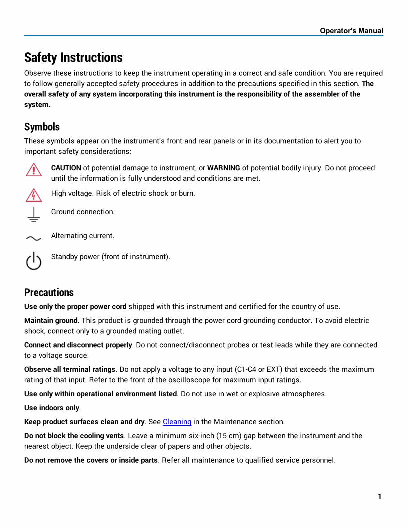
CAUTION of potential damage to instrument, or WARNING of potential bodily injury. Do not proceeduntil the information is fully understood and conditions are met.
High voltage. Risk of electric shock or burn.
Ground connection.
Alternating current.
Standby power (front of instrument).
PrecautionsUse only the proper power cord shipped with this instrument and certified for the country of use.
Maintain ground. This product is grounded through the power cord grounding conductor. To avoid electricshock, connect only to a grounded mating outlet.
Connect and disconnect properly. Do not connect/disconnect probes or test leads while they are connectedto a voltage source.
Observe all terminal ratings. Do not apply a voltage to any input (C1-C4 or EXT) that exceeds the maximumrating of that input. Refer to the front of the oscilloscope for maximum input ratings.
Use only within operational environment listed. Do not use in wet or explosive atmospheres.
Use indoors only.
Keep product surfaces clean and dry. See Cleaning in the Maintenance section.
Do not block the cooling vents. Leave a minimum six-inch (15 cm) gap between the instrument and thenearest object. Keep the underside clear of papers and other objects.
Do not remove the covers or inside parts. Refer all maintenance to qualified service personnel.
1

WaveSurfer 10 Oscilloscopes
Do not operate with suspected failures. Do not use the product if any part is damaged. Obviously incorrectmeasurement behaviors (such as failure to calibrate) might indicate impairment due to hazardous liveelectrical quantities. Cease operation immediately and sequester the instrument from inadvertent use.
Operating EnvironmentTemperature: 5 to 40° C.
Humidity: Maximum relative humidity 80 % for temperatures up to 31° C, decreasing linearly to 50% relativehumidity at 40° C.
Altitude: Up to 3,000 m at or below 25° C.
CoolingThe instrument relies on forced air cooling with internal fans and vents. Take care to avoid restricting theairflow to any part. Around the sides and rear, leave a minimum of 15 cm (6 inches) between the instrumentand the nearest object. The feet provide adequate bottom clearance.
CAUTION. Do not block cooling vents. Always keep the area beneath the instrument clear of paperand other items.
The instrument also has internal fan control circuitry that regulates the fan speed based on the ambienttemperature. This is performed automatically after start-up.
Power
AC PowerThe instrument operates from a single-phase, 100-240 Vrms (± 10%) AC power source at 50/60 Hz (± 5%) or a100-120 Vrms (± 10%) AC power source at 400 Hz (± 5%). Manual voltage selection is not required becausethe instrument automatically adapts to the line voltage.
Power ConsumptionMaximum power consumption with all accessories installed (e.g., active probes, USB peripherals) is 340 W(340 VA). Power consumption in standby mode is 10 W.
GroundThe AC inlet ground is connected directly to the frame of the instrument. For adequate protection againelectric shock, connect to a mating outlet with a safety ground contact.
WARNING. Only use the power cord provided with your instrument. Interrupting the protectiveconductor inside or outside the oscilloscope, or disconnecting the safety ground terminal, createsa hazardous situation. Intentional interruption is prohibited.
2
Operator's Manual
Start Up
Carrying and Placing the OscilloscopeThe oscilloscope’s case contains a built-in carrying handle. Lift the handle away from the oscilloscope body,grasp firmly and lift the instrument. Always unplug the instrument from the power source before moving it.
Place the instrument where it will have a minimum 15 cm (6 inch) clearance from the nearest object. Besure there are no papers or other debris beneath the oscilloscope or blocking the cooling vents.
CAUTION. Do not place the instrument so that it is difficult to reach the power cord in case youneed to quickly disconnect from power.
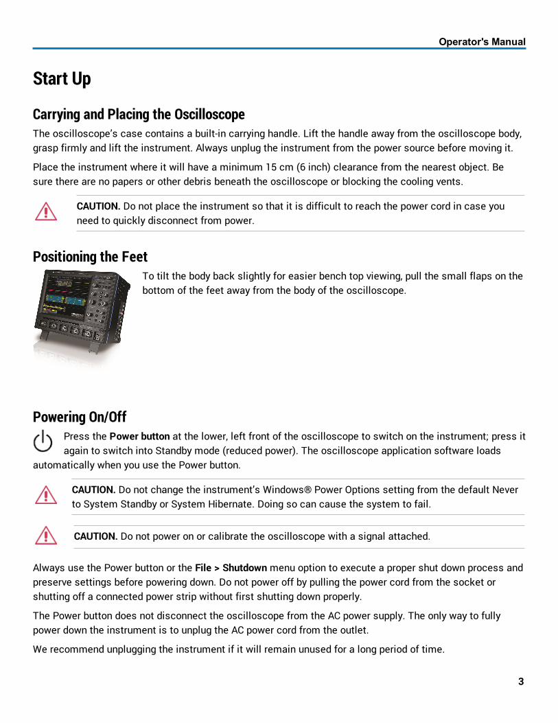
Positioning the FeetTo tilt the body back slightly for easier bench top viewing, pull the small flaps on thebottom of the feet away from the body of the oscilloscope.
Powering On/OffPress the Power button at the lower, left front of the oscilloscope to switch on the instrument; press itagain to switch into Standby mode (reduced power). The oscilloscope application software loads
automatically when you use the Power button.
CAUTION. Do not change the instrument’s Windows® Power Options setting from the default Neverto System Standby or System Hibernate. Doing so can cause the system to fail.
CAUTION. Do not power on or calibrate the oscilloscope with a signal attached.
Always use the Power button or the File > Shutdown menu option to execute a proper shut down process andpreserve settings before powering down. Do not power off by pulling the power cord from the socket orshutting off a connected power strip without first shutting down properly.
The Power button does not disconnect the oscilloscope from the AC power supply. The only way to fullypower down the instrument is to unplug the AC power cord from the outlet.
We recommend unplugging the instrument if it will remain unused for a long period of time.
3

WaveSurfer 10 Oscilloscopes
Software ActivationThe oscilloscope operating software (firmware and standard applications) is active upon delivery. At power-up, the oscilloscope loads the software automatically.
FirmwareFree firmware updates are available periodically from the Teledyne LeCroy website at:
teledynelecroy.com/support/softwaredownload.
Registered users can receive an email notification when a new update is released. Follow the instructionson the website to download and install the software.
Purchased OptionsIf you decide to purchase an option, you will receive a license key via email that activates the optionalfeatures on the oscilloscope. See Adding an Option Key for instructions on activating optional softwarepackages.
Front Input/Output Panel
A. Power button.
B. Channel inputs 1-4 for analog signals.
C. EXT to input an external trigger.
D. Front-mounted host USB port for transferring data or connecting peripherals such as a mouse orkeyboard.
E. Ground and calibration output terminal used to compensate passive probes.
4

Operator's Manual
Analog InputsA series of BNC connectors arranged on the front of the are used to input analog signal on Channels 1-4.
Channel connectors use the ProBus interface. The ProBus interface contains a 6-pin power andcommunication connection and a BNC signal connection to the probe. It includes sense rings for detectingpassive probes and accepts a BNC cable connected directly to it. ProBus offers 50 Ω and 1 MΩ inputimpedance and control for a wide range of probes.
The interfaces power probes and completely integrate the probe with the oscilloscope channel. Uponconnection, the probe type is recognized and some setup information, such as input coupling andattenuation, is performed automatically. This information is displayed on the Probe Dialog, behind theChannel (Cx) dialog. System (probe plus oscilloscope) gain settings are automatically calculated anddisplayed based on the probe attenuation.
ProbesWaveSurfer 10 oscilloscopes are compatible with the included passive probes and all Teledyne LeCroyProBus active probes that are rated for the oscilloscope’s bandwidth. Probe specifications anddocumentation are available at teledynelecroy.com/probes.
The passive probes supplied with your oscilloscope are matched to the input impedance of the instrumentbut may need further compensation. Follow the directions in the probe instruction manual to compensate thefrequency response of the probes.
Digital Inputs
The WaveSurfer 10 is compatible with the MS-250 and MS-500 Mixed Signal hardware options for input of up-to-36 lines of digital data. For instructions, see the product documentation available fromteledynelecroy.com.
5

WaveSurfer 10 Oscilloscopes
Side Input/Output PanelA. Audio Input/Output Line-In, Speaker, and Mic jacks connect the
oscilloscope to external audio devices.
B. Ethernet Port connects the oscilloscope to networks.
C. USB Ports (4) allow you to connect external USB devices, such asstorage drives.
D. L-BUS connector interfaces the oscilloscope with the MS-250 or MS-500external MSO module.
E. VGAconnector sends video output to external monitors.
6

Operator's Manual
Connecting to Other Devices/SystemsMake all desired cable connections. After start up, configure the connections using the menu options listedbelow. More detailed instructions are provided later in this manual.
POWER
Connect the line cord rated for your country to the AC power inlet on the back of the instrument, then plug itinto a grounded AC power outlet. (See Power and Ground Connections in General Safety Information.)
LANThe instrument accepts DHCP network addressing. Connect a cable from the Ethernet port on the side panelto a network access device.
To assign the oscilloscope a static IP address, go to Utilities > Utilities Setup > Remote and choose NetConnections from the Remote dialog. Use the standard Windows networking dialogs to configure the deviceaddress.
Go to Utilities > Preference Setup > Email to configure email settings.
USB PERIPHERALS
Connect the device to a USB port on the front or side of the instrument.
PRINTER
The oscilloscope supports USB printers compatible with the oscilloscope's Windows OS. Connect the printerto any host USB port. Go to Utilities > Utilities Setup > Hardcopy to configure printer settings.
EXTERNAL MONITOR
Connect the monitor cable to the VGA output on the sideof the instrument. Minimize the oscilloscopeapplication and use the Windows controls to configure the display. Configure the oscilloscope as the primarymonitor and be sure to extend, not duplicate, the display.
EXTERNAL CONTROLLERConnect a USB-A/B cable from the instrument to the controller, or connect both to the same network usingan Ethernet connection. Go to Utilities > Preference Setup > Remote to configure remote control.
OTHER AUXILIARY DEVICE
Connect a BNC cable from Aux Out on the back of the instrument to the other device. Go to Utilities >Utilities Setup > Aux Output to configure the output.
7

WaveSurfer 10 Oscilloscopes
Touch ScreenThe touch screen is the principal viewing and control center of the oscilloscope. The entire display area isactive: use your finger or the stylus to touch, double-touch, touch-and-drag, or draw a selection box. Manycontrols that display information also work as “buttons” to access other functions.
If you have a mouse installed, you can click anywhere you can touch to activate a control; in fact, you canalternate between clicking and touching, whichever is convenient for you.
The touch screen is divided into the following major control groups:
Menu BarThe top of the window contains a complete menu of oscilloscope functions. Making a selection herechanges the dialogs displayed at the bottom of the screen.
Many common oscilloscope operations can also be performed from the front panel or launched via theDescriptor Boxes. However, the menu bar is the best way to access dialogs for Save/Recall (File) functions,Display functions, Status, LabNotebook, Pass/Fail setup, and Utilities/Preferences setup.
8

Operator's Manual
Grid AreaThe grid area displays the waveform traces. Every grid is 8 Vertical divisions and 10 Horizontal divisions. Thevalue of Vertical and Horizontal divisions depends on the Vertical and Horizontal scale of the traces thatappear on the grid.
By default (Auto Grid mode), the grid area will automatically divide up to three times to display channel, zoomand math traces on different grids. Regardless of the number of grids, every grid always shows the samenumber of Vertical levels. Therefore, absolute Vertical measurement precision is maintained.
Different types of traces opening in a multi-grid display.
Adjusting Grid BrightnessYou can adjust the brightness of the grid lines. Go to Display > Display Setup and enter a new Grid Intensitypercentage. The higher the number, the brighter and bolder the grid lines.
Grid IndicatorsThese indicators appear around or on the grid to mark important points on the display. They are matched tothe color of the trace to which they apply.
Trigger Position, a small triangle along the bottom (horizontal) edge of the grid, shows the timethe oscilloscope is set to trigger an acquisition. Unless Delay is set, this indicator is at the zero(center) point of the grid. Trigger Delay is shown at the top right of the Timebase descriptor box.
Pre/Post-trigger Delay, a small arrow to the bottom left or right of the grid, indicates that a pre- orpost-trigger Delay has shifted the Trigger Position indicator to a point in time not displayed on thegrid. All trigger Delay values are shown on the Timebase Descriptor Box.
9

WaveSurfer 10 Oscilloscopes
Trigger Level at the right edge of the grid tracks the trigger voltage level. If you change the triggerlevel when in Stop trigger mode, or in Normal or Single mode without a valid trigger, a hollowtriangle of the same color appears at the new trigger level. The trigger level indicator is not shownif the triggering channel is not displayed.
Zero Volts Level is located at the left edge of the grid. One appears for each open trace on thegrid, sharing the number and color of the trace.
Various Cursor lines appear over the grid to indicate specific voltage and time values on thewaveform. Touch-and-drag cursor indicators to quickly reposition them.
Grid Context MenuQuickly touch a trace, or touch-and-hold the trace descriptor box, to open a pop-up menuwith various actions such as turning on/off the trace, placing a label, or applying mathand measurements.
Descriptor BoxesTrace descriptor boxes appear just beneath the grid whenever a trace is turned on. They function to:
l Inform—descriptors summarize the current trace settings and its activity status.
l Navigate—touch the descriptor box once to activate the trace; the box will be highlighted. Touch it asecond time to open the trace setup dialog.
Besides trace descriptor boxes, there are also Timebase and Trigger descriptor boxes summarizing theacquisition settings shared by all channels, which also open the corresponding setup dialogs.
Channel Descriptor BoxChannel trace descriptor boxes correspond to analog signal inputs. They show (clockwisefrom top left): Channel Number, Pre-Processing List, Coupling, Gain Setting, Offset Setting,Sweeps Count (when Averaging), and Vertical Cursor positions. Codes are used to indicatepre-processing that has been applied to the input. The short form is used when severalprocesses are in effect.
10

Operator's Manual
Preprocessing Symbols on Descriptor Boxes
Pre-Processing Type Long Form Short Form
Sin X Interpolation SINX S
Averaging AVG A
Inversion INV I
Deskew DSQ DQ
Coupling DC50, DC1M or AC1M D50, D1, or A1
Ground GND G
Bandwidth Limiting BWL B
Other Trace Descriptor Boxes
Similar descriptor boxes appear for math, zoom (Zx), and memory (Mx) traces. These descriptor boxes showany Horizontal scaling that differs from the signal Timebase. Units will be automatically adjusted for thetype of trace.
NOTE: On WaveSurfer 10 oscilloscopes with the WS10-ADT option installed, there will be two math functions,labeled F1 and F2 on the descriptor boxes and on the Math setup dialogs.
Timebase and Trigger Descriptor BoxThe Timebase descriptor box shows: (clockwise from top right) Trigger Delay (position), Time/div, SampleRate, Number of Samples, and Sampling Mode (blank when in real-time mode).
Trigger descriptor box shows: (clockwise from top right) Trigger Source and Coupling, Trigger Level (V),Slope, Trigger Type, Trigger Mode.
Setup information for Horizontal cursors, including the time between cursors and the frequency, is shownbeneath the TimeBase and Trigger descriptor boxes. See the Cursors section for more information.
11

WaveSurfer 10 Oscilloscopes
DialogsDialogs appear at the bottom of the display for entering setup data. The top dialog will be the main entrypoint for the selected setup option. For convenience, related dialogs appear as a series of tabs behind themain dialog. Touch the tab to open the dialog.
Right-Hand DialogsAt times, your selections will require more settings than normally appear (or can fit) on a dialog, or the taskcommonly invites further action, such as zooming a new trace. In that case, sub-dialogs will appear to theright-side of the main dialog. These right-hand dialog settings always apply to the object that is beingconfigured on the left-hand dialog.
Action ToolbarSeveral setup dialogs contain a toolbar at the bottom of the dialog. These buttons apply common actionswithout having to leave the underlying set up dialog. They always apply to the active trace.
Measure opens the Measure pop-up to set measurement parameters on the active trace.
Zoom creates a zoom trace of the active trace.
Math opens the Math pop-up to apply math functions to the active trace and create a new math trace.
Decode opens the main Serial Decode dialog where serial data decoders can be configured and applied. Thisbutton is only active if you have decoder software options installed.
Store loads the active trace into the corresponding memory location (C1, F1 and Z1 to M1; C2, F2 and Z2 toM2, etc.).
Find Scale automatically performs a vertical scaling that fits the waveform into the grid.
Label opens the Label pop-up to annotate the active trace.
12

Operator's Manual
Turning On/Off Traces
Analog TracesFrom the menu bar, choose Vertical > Channel <#> Setup to turn on the trace. To turn it off, clear the TraceOn checkbox on the corresponding Channel dialog, or touch-and-hold (right-click) on the descriptor box andchoose Off.
From the front panel, press the Channel button (1-4) to turn on the trace; press again to turn it off.
NOTE: The default is to display each trace type in its own grid (e.g., Channels together, Zooms together, etc.).Use the Display menu to change how traces are arranged.
Other TracesQuickly create zoom or math traces by touching the Zoom or Math action toolbar button.
Activate TraceAlthough several traces may be open and appear on the grid, only one at a time is active. Touch the tracedescriptor box to activate the trace. A highlighted descriptor box indicates the trace is active. All actions nowapply to that trace until you activate another.
Active trace descriptor (left), inactive trace descriptor (right).
Whenever you activate a trace, the dialog at the bottom of the screen automatically switches to theappropriate setup dialog. The tab at the top of the dialog shows to which trace it belongs.
Channel descriptor label matches Channel dialog tab.
13

WaveSurfer 10 Oscilloscopes
Annotating TracesThe Label function gives you the ability to add custom annotations to traces that are shownon the display. Labels are numbered sequentially in the order they were created. Onceplaced, labels can be moved to new positions or turned off.
Create Label1. Touch the trace and choose Set label... from the context menu, or touch the trace descriptor box twice
and touch the Label toolbar button on the setup dialog.
2. On the Trace Annotation pop-up, touch Add Label.
3. Enter the Label Text.
4. Optionally, enter the Horizontal Pos. and Vertical Pos. (in same units as the trace) at which to place thelabel. The default position is 0 ns horizontal. You can optionally check Use Trace Vertical Positioninstead of entering a Vertical Pos.
Reposition LabelOnce placed, drag-and-drop labels to a new position on the grid, or reopen the Trace Annotation pop-up andenter a new Horizontal Pos. and Vertical Pos.
Edit/Remove LabelOpen the Trace Annotation pop-up and select the Label. You can use the Up/Down arrow keys to scroll thelist. Change the Label Text or Horizontal and Vertical Pos.(itions). Touch Remove Label to delete it.
Turn On/Off LabelsAfter labels have been placed, you can turn on/off all labels at once by opening the Trace Annotation dialogand selecting/deselecting the View labels checkbox.
14

Operator's Manual
Entering/Selecting DataTouch
Touch once to activate a control. In some cases, you’ll immediately see a pop-up menu ofoptions. Touch one to select it.
TIP: You can touch the Icon or List buttons where they appear on largerpop-ups to change how menu options are displayed.
Touch & TypeIn other cases, data entry fields appear highlighted in blue when you touch them. When adata entry field is highlighted, it is active and can be modified by using the front panelAdjust knob. Or, touch it again and use the pop-up menu or keypad to make an entry.
You’ll see a pop-up keypad when you touch twice on a numerical dataentry field. Use it exactly as you would a calculator. When you touchOK, the calculated value is entered in the field.
The Set to... buttons quickly enter the maximum, default or minimumvalue for that field.
The Up and Down arrow buttons increment/decrement the displayedvalue.
The Variable checkbox allows you to make fine increment changeswhen using the Up and Down arrow buttons.
15

WaveSurfer 10 Oscilloscopes
Touch & DragTouch-and-drag cursor lines and annotation labels toreposition them on the grid; this is the same as setting thevalues on the dialog.
Touch-and-drag to draw a selection box around part of a traceto quickly zoom that portion.
Printing/Screen CaptureThe Print function captures an image of the display and outputs it according to your Hardcopy settings.
There are three ways to print a capture of the screen:
l Touch the front panel Print button.
l Choose File > Print.
l Choose Utilities > Utilities Setup > Hardcopy tab and touch the Print button to the far right of thedialog.
NOTE: When the front panel Print button is configured to capture the screen as a LabNotebook entry, only theFile and Utilities menu print options will function according to your Hardcopy setup.
16
Operator's Manual
Oscilloscope Application WindowThe oscilloscope application runs on a Windows operating system and functions exactly as do otherWindows applications.
To minimize the application window and show the Windows desktop, choose File > Minimize. To restore thewindow after minimizing, touch the oscilloscope display icon in the lower right corner of the desktop.
To exit the application window, choose File > Exit. When you exit the application, the oscilloscope operatingsystem continues to run. To reload the application after exiting, touch the Start DSO desktop shortcut.
Language SelectionTo change the language that appears on the touch screen:
1. Go to Utilities > Preference Setup > Preferences and make your Language selection.
2. Follow the prompt to restart the oscilloscope application.
To also change the language of the Windows operating system dialogs:
1. Choose File > Minimize to hide the oscilloscope display and show the Windows Desktop.
2. From the Windows task bar, choose Start > Control Panel > Clock, Language and Region.
3. Under Region and Language select Change Display Language.
4. Touch the Install/Uninstall Languages button.
5. Select Install Language and Browse Computer or Network.
6. Touch the Browse button, navigate to D:\Lang Packs\ and select the language you want to install. Theavailable languages are: German, Spanish, French, Italian, and Japanese. Follow the installer prompts.
NOTE: Other language packs are available from Microsoft’s website.
7. Reboot the oscilloscope after changing the language.
Screen SaverAs on any Windows PC, a screen saver can be enabled to begin after a preset idle time, or disabled:
1. Minimize the oscilloscope application by choosing File > Minimize from the menu bar.
2. Open the Windows Control Panel to change Appearance and Personalization settings.
3. Touch the oscilloscope icon at the bottom right of the desktop to restore the instrument display.
17

WaveSurfer 10 Oscilloscopes
Front PanelMost front panel controls duplicate functionality available through thetouch screen display and are described on the following pages.
Many knobs on the front panel function one way if turned and anotherif pushed like a button. When a knob is multi-plexed, the top labeldescribes the knob’s “turn” action, the bottom label its “push” action.
Front panel buttons light up to indicate which traces and functions areactive. Actions performed from the front panel always apply to theactive trace.
Top Row ButtonsAuto Setup performs an Auto Setup. After the first press, you will beprompted for a confirmation. Press the button again or use the touchscreen to confirm.
Clear Sweeps resets the acquisition counter and any cumulativemeasurements.
Print captures the entire screen and outputs it according to yourHardcopy settings. It can also be configured to output a LabNotebookentry.
When you push the Intensity knob, the oscilloscope switches intoWaveStream acquisition mode. The WaveStream indicator lights toshow it is on.
Trigger ControlsLevel knob changes the trigger threshold level (V). The number is
shown on the Trigger descriptor box. Pushing the knob sets the trigger level to the 50% point of the inputsignal.
READY indicator lights when the trigger is armed. TRIG'D is lit momentarily when a trigger occurs. A fasttrigger rate causes the light to stay lit continuously.
Setup corresponds to the menu selection Trigger > Trigger Setup. Press it once to open the Trigger Setupdialog and again to close the dialog.
Auto sets Auto trigger mode, which triggers the oscilloscope after a time-out, even if the trigger conditionsare not met.
Normal sets Normal trigger mode, which triggers the oscilloscope each time a signal is present that meetsthe conditions set for the type of trigger selected.
18

Operator's Manual
Single sets Single trigger mode, which arms the oscilloscope to trigger once (single-shot acquisition) whenthe input signal meets the trigger conditions set for the type of trigger selected. If the scope is alreadyarmed, it will force a trigger.
Stop prevents the oscilloscope from triggering on a signal. If you boot up the instrument with the trigger inStop mode, a "No trace available" message is shown. Press the Auto button to display a trace.
Horizontal ControlsThe Delay knob changes the Trigger Delay value (S) when turned. Push the knob to reset Delay to zero.
The Horizontal Adjust knob sets the Time/division (S) of the oscilloscope acquisition system when the tracesource is an input channel. The Time/div value is shown on the Timebase descriptor box. When using thiscontrol, the oscilloscope allocates memory as needed to maintain the highest sample rate possible for thetimebase setting. When the trace is a zoom, memory or math function, turn the knob to change the horizontalscale of the trace, effectively "zooming" in or out. By default, the knob adjusts values in 1, 2, 5, 10 stepincrements. Push the knob to change the action to fine increments; push it again to return to steppedincrements.
Vertical ControlsChannel buttons turn on a channel that is off, or activate a channel that is already on. When the channel isactive, pushing its channel button turns it off. A lit button shows the active channel.
Offset knob adjusts the zero level of the trace (this makes it appear to move up or down relative to thecenter axis of the grid). The value appears on the trace descriptor box. Push it to reset Offset to zero.
Gain knob sets Vertical Gain (V/div). The value appears on the trace descriptor box. By default, the knobadjusts values in 1, 2, 5, 10 step increments. Push the knob to change the action to fine increments; push itagain to return to stepped increments.
Measure, Zoom, and Mem(ory) ButtonsThe Zoom button creates a quick zoom for each open channel trace. Touch the zoom trace descriptor box todisplay the zoom controls.
The Measure and Mem(ory) buttons open the corresponding setup dialogs.
Cursor ControlsCursors identify specific voltage and time values on the waveform. The white cursor lines help make thesepoints more visible, while a readout of the values appears on the trace descriptor box. There are three presetcursor types, each with a unique appearance on the display. These are described in more detail in theCursors section.
Type selects the cursor type. Continue pressing to cycle through all cursor types until the desired type isfound. The type "no cursors" turns off the cursor display.
19

WaveSurfer 10 Oscilloscopes
Cursor knobs reposition the selected cursor line when turned. Each knob controls one line. Push the knobresets the cursor to the default position. When both Horizontal and Vertical cursors are displayed, each knobcontrols two lines, and pushing the knob switches the line that is being controlled.
AdjustThe Adjust knob changes the value in any highlighted data entry field when turned. Pushing the Adjust knobtoggles between coarse (large increment) or fine (small increment) adjustments when the knob is turned.
The Touch Screen button enables/disables the touch screen controls.
20

Operator's Manual
Zooming WaveformsThe Zoom function magnifies a selected region of a trace. On WaveSurfer 10 model oscilloscopes, you candisplay up to four zoom traces (Z1-Z4) taken from any channel, math, or memory trace.
Creating ZoomsTo create a zoom, touch -and-drag to draw a selection box around any part of the source waveform.
Selection box over trace.
The zoom will resize the selected portion to fit the full width of the grid. The degree of vertical and horizontalmagnification, therefore, depends on the size of the rectangle that you draw.
The zoom opens in a new grid, with the zoomed portion of the source trace highlighted. New zooms areturned on and visible by default. However, you can turn off a particular zoom if the display becomes toocrowded, and the zoom settings are saved in its Zx location, ready to be turned on again when desired.
21

WaveSurfer 10 Oscilloscopes
Adjust ZoomThe zoom's Horizontal units will differ from the signal timebase because the zoom is showing a calculatedscale, not a measured level. This allows you to adjust the zoom factor using the front panel knobs or theZoom dialog controls however you like without affecting the timebase (a characteristic shared with mathand memory traces).
Turn off ZoomTo close the zoom, either touch the zoom descriptor box twice to open the Zoom dialog and deselect TraceOn, or touch the zoom trace to open the context menu and choose Off.
Zoom ControlsTo open the Zoom dialog, touch twice on any zoom descriptor box, or choose Math > Zoom Setup from themenu bar.
Trace ControlsTrace On shows/hides the zoom trace. It is selected by default when the zoom is created.
Source lets you change the source for this zoom to any channel, math, or memory trace while maintaining allother settings.
Segment ControlsThese controls are used in Sequence Sampling Mode. They are only displayed on WaveSurfer 10oscilloscopes with the WS10-ADT option installed.
Zoom Factor ControlsThese controls on the Zx dialogs appear throughout the oscilloscope software:
l Out and In buttons increase or decrease the magnification of the zoom, and consequently change theHorizontal and Vertical Scale settings. Continue to touch either button until you've achieved the desiredlevel of zoom.
22

Operator's Manual
l Var. checkbox enables variable zooming in increments finer than the default 1, 2, 5, 10 stepincrements. When checked, each touch of the zoom control buttons changes the degree ofmagnification by a single increment.
l Horizontal Scale/div sets the amount of time represented by each horizontal division of the grid. It isthe equivalent of Time/div, only unlike the Timebase setting, it may be set differently for each zoom,math function, or memory trace.
l Vertical Scale/div sets the voltage level represented by each vertical division of the grid; it's theequivalent of V/div used for channel settings.
l Horizontal/Vertical Center sets the voltage or time that is to be at the center of the screen on the zoomtrace. The horizontal center is the same for all zoom traces.
l Reset Zoom returns the zoom to x1 magnification.
23

WaveSurfer 10 Oscilloscopes
VerticalVertical, also called Channel, settings usually relate to voltage level and control the trace along the Y axis.
The amount of voltage displayed by one vertical division of the grid, or Vertical Scale (V/div), is most quicklyadjusted by using the front panel Vertical knob. The Channel descriptor box always shows the currentVertical Scale setting.
Vertical settings are made on the Channel dialog, labeled Cx after the corresponding channel. To access theChannel dialog, choose Vertical > Channel <#> Setup from the menu bar, or touch the Channel descriptor box.
The Cx dialog contains:
l Channel Settings for scale, offset, coupling, bandwidth, and probe attenuation.
l Pre-Processing Settings to set up pre-acquisition processes that will affect the waveform, such asnoise filtering and interpolation.
If a Teledyne LeCroy probe is connected to the channel, a Probe dialog appears behind the Cx dialog.
Channel Settings
Volts/div sets the vertical scale (aka gain or sensitivity). Select Variable Gain adjustment or leave thecheckbox clear for fixed adjustment.
Offset adds a defined value of DC offset to the signal as acquired by the input channel. This may helpful inorder to display a signal on the oscilloscope grid while maximizing the vertical height (or gain) of the signal.A negative value of offset will "subtract" a DC voltage value from the acquired signal (and move the tracedown on the grid") whereas a positive value will do the opposite. Touch Zero Offset to return to zero.
A variety of Bandwidth filters are available at a variety of fixed settings. The exact settings vary by model. Tolimit bandwidth, select a filter from this field.
Invert inverts the waveform for the selected channel.
Coupling may be set to DC 50 Ω, DC1M, AC1M or GROUND (Gnd).
CAUTION. The maximum input voltage depends on the input used. Limits are displayed on the frontof the oscilloscope. Whenever the voltage exceeds this limit, the coupling mode automatically
24

Operator's Manual
switches to GROUND. You then have to manually reset the coupling to its previous state. While theunit does provide this protection, damage can still occur if extreme voltages are applied.
Deskew adjusts the amount of horizontal time offset to compensate for propagation delays caused bydifferent probes or cable lengths. The valid range depends on the current timebase setting. The Mathdeskew function performs the same activity.
Probe SettingsWhen a Teledyne LeCroy-compatible probe is connected to the oscilloscope input, the probe is automaticallyidentified and the model name displayed on the Channel dialog under the "Probe" heading. Also, the Probedialog bearing the probe name is added to the right of the Channel dialog. When a probe is not connected, theChannel dialog shows only the Cx tab for vertical setup.
When third-party probes are connected, an Attenuation field appears on the Cx dialog, with a default value of/1, allowing you to enter attenuation and rescale values manually.
Channel dialog with tab for connected probe.
The Probe Dialog displays probe attributes and (depending on the probe type) allows you to AutoZero orDeGauss probes from the oscilloscope touch screen. Other settings may appear, as well, depending on theprobe model.
Probe dialog showing the connected probe's control attributes.
25

WaveSurfer 10 Oscilloscopes
Auto Zero ProbeAuto Zero corrects for DC offset drifts that naturally occur from thermal effects in the amplifier of activeprobes. Teledyne LeCroy probes incorporate Auto Zero capability to remove the DC offset from the probe'samplifier output to improve the measurement accuracy.
CAUTION. Remove the probe from the circuit under test before initializing Auto Zero.
DeGauss ProbeThe Degauss control is activated for some types of probes (e.g., current probes). Degaussing eliminatesresidual magnetization from the probe core caused by external magnetic fields or by excessive input. It isrecommended to always degauss probes prior to taking a measurement.
CAUTION. Remove the probe from the circuit under test before initializing DeGauss.
Auto SetupAuto Setup quickly configures the essential oscilloscope settings based on the first input signal it finds,starting with Channel 1. If nothing is connected to Channel 1, it searches Channel 2 and so forth until it findsa signal. Vertical Scale (V/div), Offset, Timebase (Time/div), and Trigger are set to an Edge trigger on thefirst, non-zero-level amplitude, with the entire waveform visible for at least 10 cycles over 10 horizontaldivisions.
To run Auto Setup:
1. Either press the Auto Setup button on the front panel, or choose Auto Setup from the Vertical, Timebase,or Trigger menus. All these options perform the same function.
2. Press the Auto Setup button again or use the touch screen display to confirm Auto Setup.
Restore Default SetupRestore the oscilloscope to its factory default state by pressing the front panel Default Setup button. Youcan also restore default settings by choosing File > Recall Setup > Recall Default.
Default settings for your oscilloscope include the following:
Channel/Vertical C1-C2 on at 50 mV/div Scale, 0 V Offset
Timebase Real Time Sampling at 50 ns/div, 0 Delay, 2.0 kS at 4 GS/s, 100 kS Memory
Trigger C1 with an Auto Positive Edge, DC Coupling, 0 V Level
Display Auto Grid
Cursors Off
Measurements Cleared
Math Cleared
26

Operator's Manual
Viewing StatusAll oscilloscope settings can be viewed through the various Status dialogs. These show all existingacquisition, trigger, channel, math function, measurement and parameter configurations, as well as whichare currently active.
Access the Status dialogs by choosing the Status option from the Vertical, Timebase, Math menus (e.g.,Channel Status, Acquisition Status).
27

WaveSurfer 10 Oscilloscopes
TimebaseTimebase, also known as Horizontal, settings control the trace along the X axis. The timebase is shared byall channels.
The time represented by each horizontal division of the grid, or Time/Division, is most easily adjusted usingthe front panel Horizontal knob. Full Timebase set up, including sampling mode selection, is done on theTimebase dialog, which can be accessed by either choosing Timebase > Horizontal Setup from the menu bar,or touching the Timebase descriptor box.
The Timebase dialog contains settings for Sampling Mode, Timebase Mode, Real Time Memory, and ActiveChannels.
Timebase Settings
Sampling ModeChoose fromWaveStream, Real Time, Sequence,RIS, orRoll mode.
NOTE: Sequence mode available only on oscilloscopes with the WS10-ADT option installed.
Timebase ModeTime/Division is the time represented by one horizontal division of the grid. Touch the Up/Down Arrowbuttons on the Timebase dialog or turn the front panel Horizontal knob to adjust this value.
Delay is the amount of time relative to the trigger event to display on the grid. In Real Time sampling mode,the trigger event is placed at time zero on the grid. Delay may be time pre-trigger, entered as a negativevalue, or post-trigger, entered as a positive value. Raising/lowering the Delay value has the effect of shiftingthe trace to the right/left, enabling you to focus on the relevant portion of longer acquisitions.
Set to Zero returns Delay to zero.
Real Time MemoryMax. Sample Points is the maximum number of samples taken per acquisition. The actual number ofsamples acquired can be lower due to the current Sample Rate and Time/Division settings.
28

Operator's Manual
Active ChannelsThese settings enable you to control the distribution of memory to achieve longer acquisitions through asingle channel if needed.
4 (or 2 in 2 channel scopes) utilizes the per channel maximum memory (10 Mpts/ch standard, 16 Mpts/chwith the WS10-ADT option).
2 (or 1 in 2 channel scopes) distributes the total maximum memory across only two channels (20 Mpts/chstandard, 32 Mpts/ch with the WS10-ADT option) . Channels 2 and 3 (in 4 channel scopes) and Channel 2 (in2 channel scopes) are available for use.
Auto allows the scope to make this decision based on which channels are currently in use.
Sampling Modes
WaveStream Sampling ModeWaveStream provides a vibrant, intensity graded display with a fast update rate to closely simulate the lookand feel of an analog oscilloscope. WaveStream is most helpful in viewing signals that have signal jitter orsignal anomalies, or for applying a visual check before creating an advanced trigger or WaveScan setup tolocate an unusual event.
WaveStream mode operates at up to 80 GS/s with an update rate of up to several thousandwaveforms/second for better capture of higher frequency abnormal events. Time/div must be set to 50 ms orfaster to use WaveStream.
Waveform captured in WaveStream sampling mode, showing hard-to-find runt.
To use WaveStream, select it as the Sampling Mode when making other settings on the Timebase dialog, orpress the front panel Intensity knob. The WaveStream (ACQ) indicator next to the knob will light to show youare now in WaveStream mode. Press the knob again to exit WaveStream Mode.
29

WaveSurfer 10 Oscilloscopes
Real Time Sampling ModeReal Time sampling mode is a series of digitized voltage values sampled on the input signal at a uniformrate. These samples are displayed as a series of measured data values associated with a single triggerevent. By default, the waveform is horizontally positioned so that the trigger event is time zero on the grid.
The relationship between sample rate, memory, and time can be expressed as:
Capture Interval = 1/Sample Rate X MemoryCapture Interval/10 = Time Per Division
In Real Time sampling mode, the acquisition can be displayed for a specific period of time (or number ofsamples) either before or after the trigger event occurs, known as trigger delay. This allows you to isolateand display a time/event of interest that occurs before or after the trigger event.
l Pre-trigger delay displays the time prior to the trigger event. This can be set from a time well beforethe trigger event to the moment the event occurs, up to the oscilloscope's maximum sample recordlength. How much actual time this represents depends on your timebase setting. When set to themaximum allowed pre-trigger delay, the trigger position (and zero point) is off the grid (indicated by thetrigger delay arrow at the lower right corner), and everything you see represents pre-trigger time.
l Post-trigger delay displays time following the trigger event. Post-trigger delay can cover a muchgreater lapse of time than pre-trigger delay, up to the equivalent of 10,000 time divisions after thetrigger event occurred. When set to the maximum allowed post-trigger delay, the trigger point mayactually be off the grid far to the left of the time displayed.
Usually, on fast timebase settings, the maximum sample rate is used when in Real Time mode. For slowertimebase settings, the sample rate is decreased so that the maximum number of data samples ismaintained over time.
Sequence Sampling ModeSequence sampling mode is available on WaveSurfer 10 oscilloscopes with the WS10-ADT option installed.
In Sequence Mode, the complete waveform consists of a number of fixed-size segments (see the instrumentspecifications at teledynelecroy.com for the limits). The oscilloscope uses the sequence timebase settingto determine the capture duration of each segment as 10 x time/div. With this setting, the oscilloscope usesthe desired number of segments, maximum segment length, and total available memory to determine theactual number of samples or segments, and time or points.
Sequence Mode is ideal when capturing many fast pulses in quick succession or when capturing few eventsseparated by long time periods. The instrument can capture complicated sequences of events over largetime intervals in fine detail, while ignoring the uninteresting periods between the events. You can also maketime measurements between events on selected segments using the full precision of the acquisitiontimebase.
30

Operator's Manual
SET UP SEQUENCE MODE
When setting up Sequence Mode, you define the number of fixed-size segments acquired in single-shot mode(see the instrument specifications for the limits). The oscilloscope uses the sequence timebase setting todetermine the capture duration of each segment. Along with this setting, the oscilloscope uses the numberof segments, maximum segment length, and total available memory to determine the actual number ofsamples or segments, and time or points.
1. From the menu bar, choose Timebase > Horizontal Setup....
2. Choose Sequence Sampling Mode.
3. On the Sequence tab under Acquisition Settings, touch Number of Segments and enter a value.
4. To stop acquisition in case no valid trigger event occurs within a certain timeframe, check the EnableTimeout box, then touch Timeout and provide a timeout value.
NOTE: While optional, Timeout ensures that the acquisition will complete in a reasonable amount of timeand control of the oscilloscope will return to the operator/controller without having to manually stop theacquisition.
5. Touch the one of the front panel Trigger buttons to begin acquisition.
NOTE: Once acquisition has started, you can interrupt it at any time by pressing the Stop front panelbutton. In this case, the segments already acquired will be retained in memory.
VIEW SEGMENTS IN SEQUENCE MODE
When in Sequence Mode, you can view individual segments easily using the Zoom dialog. The Zoom tracedefaults to Segment 1. You can move to later segments by changing the values in First segment to displayand Num(ber) of segments to display at once.
TIP: By changing the Num field value to 1, you can use the front panel Adjust knob to scroll through eachsegment in order.
Channel descriptor boxes indicate the total number of segments acquired. Zoom descriptor boxes show the .As with all other Zoom traces, the zoomed segments are highlighted on the source trace.
Use the to change the scale factors of the trace.
RIS Sampling ModeRIS (Random Interleaved Sampling) allows effective sampling rates higher than the maximum single-shotsampling rate. It is used on repetitive waveforms with a stable trigger. The maximum effective RIS samplingrate is achieved by making multiple single-shot acquisitions at maximum real-time sample rate. The binsthus acquired are positioned approximately 20 ps (50 GS/s) apart. The process of acquiring these bins andsatisfying the time constraint is a random one. The relative time between ADC sampling instants and theevent trigger provides the necessary variation.
31

WaveSurfer 10 Oscilloscopes
The instrument requires multiple triggers to complete an acquisition. The number depends on the samplerate: the higher the sample rate, the more triggers are required. It then interleaves these segments (asshown in the following illustration) to provide a waveform covering a time interval that is a multiple of themaximum single-shot sampling rate. However, the real-time interval over which the instrument collects thewaveform data is much longer, and depends on the trigger rate and the amount of interleaving required.
Interleaving of sample in RIS sampling mode.
Roll ModeRoll mode displays, in real time, incoming points in single-shot acquisitions that appear to "roll" continuouslyacross the screen from right to left until a trigger event is detected and the acquisition is complete. Theparameters or math functions connected to each channel are updated every time the roll mode buffer isupdated, as if new data is available. This resets statistics on every step of Roll mode that is valid because ofnew data.
Timebase must be set to 100 ms/div or slower to enable Roll mode selection. Roll mode samples at ≤ 5MS/s.
NOTE: If the processing time is greater than the acquire time, the data in memory is overwritten. In this case,the instrument issues the warning, "Channel data is not continuous in ROLL mode!!!" and rolling starts again.
History ModeHistory Mode is available on WaveSurfer 10 oscilloscopes with the WS10-ADT option installed.
History Mode allows you to review any acquisition saved in the oscilloscope's history buffer, whichautomatically stores all acquisition records until full. Not only can individual acquisitions be restored to thegrid, you can "scroll" backward and forward through the history at varying speeds to capture individual detailsor changes in the waveforms over time.
Each record is indexed and time-stamped, and you can choose to view the absolute time of acquisition or thetime relative to when you entered History Mode. In the latter case, the last acquisition is time zero, and allothers are stamped with a negative time. The maximum number of records stored depends on youracquisition settings and the size of the oscilloscope memory.
To view history:
32

Operator's Manual
1. Choose Timebase > History Mode.
2. Press the front panel History Mode button, or choose Timebase > History Mode.
3. Select View History to enable the history display, and View Table to display the index of records.Optionally, select to show Relative Times on the table.
4. Choose a single acquisition to view by entering its Index number on the dialog or selecting it from thetable of acquisitions.
OR
Use the Navigation buttons to "scroll" the history of acquisitions.
l The top row of buttons scrolls continuously and are (left to right): Fast Backward, Slow Backward,Pause, Slow Forward, Fast Forward.
l The bottom row of buttons steps one record at a time and are (left to right): Back to Start, BackOne, Go to Index (#), Forward One, Forward to End.
5. Entering History Mode automatically stops new acquisitions. To leave History Mode, restart acquisitionby pressing one of the front panel Trigger Mode buttons.
33
WaveSurfer 10 Oscilloscopes
TriggerWhile the oscilloscope is continuously sampling signal when it is turned on, it can only display up to itsmaximum memory in data samples. Triggers select an exact event/time in the waveform to display on theoscilloscope screen so that memory is not wasted on insignificant periods of the signal. For all trigger types,you can set:
l Pre-trigger or post-trigger delay—time relative to the trigger event displayed on screen (although thetrigger itself may not be visible).
l Time between sweeps—how often the display is refreshed.
Unless modified by a pre- or post-trigger delay, the trigger event occurs at point zero at the center of the grid,and an equal period of time before and after this point is shown to the left and right of it.
In addition to the trigger type, the trigger mode determines how the oscilloscope behaves in the presence orabsence of a trigger event.
Trigger capabilities include:
l Simple Triggers activated by basic waveform features such as an edge with a positive or negativeslope or width.
l Pattern Triggers that fire when a pattern condition occurs on selected input channels.
l SMART Triggers, sophisticated triggers that enable you to create basic or complex trigger conditions.Use SMART Triggers for signals with rare features, like glitches.
Trigger ModesThe trigger mode determines how the oscilloscope sweeps, or refreshes, the display. This can be set fromthe Trigger menu or from the front panel Trigger control group.
Auto mode causes the oscilloscope to sweep without a set trigger. An internal timer triggers the sweep aftera preset timeout period so that the display refreshes continuously. Otherwise, Auto functions the same asNormal when a trigger condition is found.
In Normal mode, the oscilloscope sweeps only if the input signal reaches the set trigger point. Otherwise itcontinues to display the last acquired waveform.
In Single mode, one sweep occurs each time you choose Trigger > Single or press the front panel Singlebutton.
Stop pauses sweeps until you select one of the other three modes.
34
Operator's Manual
Trigger TypesThese are the trigger types available for selection. If the trigger is part of a subgroup (e.g., Smart), firstchoose the subgroup from among the basic types to display all the trigger options.
Basic TriggersEdge triggers upon a achieving a certain voltage level in the positive or negative slope of the waveform.
Width triggers upon finding a positive- or negative-going pulse width when measured at the specified voltagelevel.
Pattern triggers upon a user-defined pattern of concurrent high and low voltage levels on selected inputs. InMixed-Signal oscilloscopes, it may be a digital logic pattern relative to high and low voltage levels on analogchannels, or just a digital logic pattern omitting any analog inputs. Likewise, if your oscilloscope does nothave digital input capability, the pattern can be set using voltage levels on analog channels alone. You canstipulate the voltage level/logic threshold for each analog or digital input independently.
TV triggers on a specified line and field in standard (PAL, SECAM, NTSC, HDTV) or custom composite videosignals.
Qualified arms the trigger on the A event, then fires on the B event. In Normal trigger mode, it automaticallyresets after the B event. The A event can be an Edge, State, Pattern, or PatState (a pattern that persists overa user-defined number of events or time). The options for the B event depend on the type of A event. If A is adigital Pattern or PatState, B can only be an Edge.
NOTE: This functionality is identical to Teledyne LeCroy's previous Qualify and State triggers, but presentedthrough a different user interface.
Smart TriggersThe Smart subgroup triggers allow you to apply Boolean logic conditions to the basic signal characteristicsof level, slope, and polarity to determine when to fire the trigger.
Interval triggers upon finding a specific interval, the time (period) between two consecutive edges of thesame polarity: positive to positive or negative to negative. Use the interval trigger to capture intervals thatfall short of, or exceed, a specified range.
Glitch triggers upon finding a pulse-width that is less than a specified time or within a specified range oftimes.
Dropout triggers when a signal loss is detected. The trigger is generated at the end of the timeout periodfollowing the last trigger source transition. It is used primarily in single-shot applications with a pre-triggerdelay.
Runt triggers when a pulse crosses a first threshold, but fails to cross a second threshold before re-crossingthe first. Other defining conditions for this trigger are the edge (triggers on the slope opposite to thatselected) and runt width.
35
WaveSurfer 10 Oscilloscopes
SlewRate triggers when the rising or falling edge of a pulse crosses an upper and a lower level. The pulseedge must cross the thresholds faster or slower than a selected period of time.
Serial TriggersThe Serial trigger type will appear if you have installed protocol-specific serial data trigger and decodeoptions. Select this type to open the serial trigger setup dialogs. Instructions for using all serial data optionsare available from our website at teledynelecroy.com/serialdata.
Setting Up TriggersTo access the Trigger setup dialogs, do one of the following:
l Choose Trigger > Trigger Setup from the menu bar
l Press the front panel Trigger Setup button
l Touch the Trigger descriptor box
The main Trigger dialog contains the trigger type selections. On oscilloscopes with the Mixed Signal option,many trigger types can be set on either analog channels, including the External Trigger input, or digital lines.For digital triggering instructions, see the Operator's Manual for your Mixed Signal accessory.
Other controls will appear depending on the trigger type selection (e.g., Slope for Edge triggers). These aredescribed in the set up procedures for each trigger.
The trigger condition is summarized in a preview window at the far right of the Trigger dialog. Refer to this toconfirm your selections are producing the trigger you want.
36

Operator's Manual
Edge TriggerEdge triggers upon a achieving a certain voltage level in the positive or negative slope of the waveform. It isthe default trigger selection on standard oscilloscopes.
NOTE: Alternatively, you may choose a Slope of Window and enter the Upper Level and Lower Level voltagethat define the window. The trigger fires when the signal leaves the widow.
On the Trigger dialog, select Edge trigger type to display the controls.
1. Choose the Source signal input.
2. Enter the voltage Level upon which to trigger.
The Find Level button sets the Level to the signal mean.
3. Choose the Slope (edge) of the wave on which to trigger.
4. Choose the type of signal Coupling at the input. Choices are:
l DC - All the signal’s frequency components are coupled to the trigger circuit for high frequencybursts or where the use of AC coupling would shift the effective trigger level.
l AC - The signal is capacitively coupled. DC levels are rejected, and frequencies below 50 Hz areattenuated.
l LFREJ - The signal is coupled through a capacitive high-pass filter network, DC is rejected andsignal frequencies below 50 kHz are attenuated. For stable triggering on medium to high frequencysignals.
l HFREJ - Signals are DC coupled to the trigger circuit, and a low-pass filter network attenuatesfrequencies above 50 kHz (used for triggering on low frequencies).
37

WaveSurfer 10 Oscilloscopes
Width TriggerWidth triggers upon finding a positive- or negative-going pulse width when measured at the specified voltagelevel.
On the Trigger dialog, select Width trigger type to display the controls.
1. Choose the Source input.
2. Choose the type of signal Coupling at the input. Choices are:
l DC - All the signal’s frequency components are coupled to the trigger circuit for high frequencybursts or where the use of AC coupling would shift the effective trigger level.
l AC - The signal is capacitively coupled. DC levels are rejected, and frequencies below 50 Hz areattenuated.
l LFREJ - The signal is coupled through a capacitive high-pass filter network, DC is rejected andsignal frequencies below 50 kHz are attenuated. Best used for stable triggering on medium to highfrequency signals.
l HFREJ - Signals are DC coupled to the trigger circuit, and a low-pass filter network attenuatesfrequencies above 50 kHz. Best used for triggering on low frequencies.
3. Choose the Polarity at which to measure pulse width.
4. Enter the voltage Level at which to measure pulse width. The Find Level button sets the level to thesignal mean.
5. Use Width Condition is settings to create an expression describing the triggering pulse width. This maybe:
l Any width Less Than an Upper Value.
l Any width Greater Than a Lower Value.
l Any width In Range or Out Range of values. You may describe the range using either:
l Limits, an absolute Upper Value and Lower Value.
l Delta, any Nominal width plus or minus a Delta width.
38

Operator's Manual
Qualified TriggerQualified arms the trigger on the A event, then fires on the B event. In Normal trigger mode, it automaticallyresets after the B event. The options for the B event depend on the type of A event. You may apply additionalHoldoff by time or number of events.
On the Trigger dialog, select Qualified trigger type to display the controls.
Besides an Edge or Pattern trigger, two special conditions may be selected as the arming ("A") event:
l State, any voltage measured above or below a threshold Level.
l PatState, a pattern that persists over a user-defined number of events or time. Like Pattern triggers,PatState events may be analog voltage patterns, digital logic patterns, or a mix of both, depending onthe oscilloscope's capabilities.
NOTE: On a standard oscilloscope, Pattern and PatState events will default to the analog pattern setupdialog. On a Mixed-Signal oscilloscope, Pattern and PatState events will default to the digital pattern setupdialog.
Once you've selected the A and B events on the Qualified dialog, set up the conditions on the respective sub-dialogs exactly as you would a single-stage trigger.
39

WaveSurfer 10 Oscilloscopes
Pattern TriggerPattern is the default trigger when the Mixed Signal option is connected to the oscilloscope, as these usersgenerally wish to find and trigger upon digital logic patterns.
However, a Pattern trigger can also be set on a user-defined pattern of High or Low voltage levels in analogchannels (including the External Trigger input), or a combination of digital and analog patterns when MixedSignal capabilities are available.
See the MS-250 Operator's Manual or MS-500 Operator's Manual delivered with your Mixed Signal option forinstructions on setting up a digital pattern trigger.
To set up an analog pattern trigger, on the Trigger dialog, select Pattern trigger type.
The standard dialog for setting up an analog Pattern trigger includes all the controls for setting the patternand the voltage threshold on the same dialog.
1. Select the Boolean Operator (AND, NAND, OR, or NOR) that describes the relationship among analoginputs (e.g., C1 must be High NAND C2 must be Low).
2. For each input to be included in the trigger pattern, and select what State it must be in (High, Low, orDon't Care) compared to the threshold Level you will set. Leave "Don't Care" selected for any input youwish to exclude.
3. For each input included in the trigger, enter the voltage threshold Level.
4. If you've included EXTERNAL as an input, open the Ext tab and enter the Attenuation.
40

Operator's Manual
TV TriggerTV triggers on a specified line and field in standard (PAL, SECAM, NTSC, HDTV) or custom composite videosignals.
On the Trigger dialog, select TV trigger type to display the controls.
1. Choose the Source signal input.
2. Choose the signal TV Standard. To use a custom signal, also enter the:
l Frame Rate
l # of Fields per line
l # of Lines
l Interlace ratio
3. Choose the Line and Field upon which to trigger.
41

WaveSurfer 10 Oscilloscopes
Glitch TriggerGlitch triggers upon finding a pulse-width that is less than a specified time or within a specified range oftimes.
On the Trigger dialog, select Smart trigger type, then Glitch to display the controls.
1. Choose the Source signal input.
2. Choose the type of signal Coupling at the input. Choices are:
l DC - All the signal’s frequency components are coupled to the trigger circuit for high frequencybursts or where the use of AC coupling would shift the effective trigger level.
l AC - The signal is capacitively coupled. DC levels are rejected, and frequencies below 50 Hz areattenuated.
l LFREJ - The signal is coupled through a capacitive high-pass filter network, DC is rejected andsignal frequencies below 50 kHz are attenuated. For stable triggering on medium to high frequencysignals.
l HFREJ - Signals are DC coupled to the trigger circuit, and a low-pass filter network attenuatesfrequencies above 50 kHz (used for triggering on low frequencies).
3. Choose the Polarity on which to trigger.
4. Enter the voltage Level at which to measure. The Find Level button sets the Level to the signal mean.
5. Use Glitch Condition is settings to create an expression describing the glitch width. This may be:
l Any width Less Than an Upper Value.
l Any width In Range of values marked by the specified Upper Value and Lower Value.
42

Operator's Manual
Interval TriggerInterval triggers upon finding a specific interval, the time (period) between two consecutive edges of thesame polarity: positive to positive or negative to negative. Use the interval trigger to capture intervals thatfall short of, or exceed, a specified range.
On the Trigger dialog, select Smart trigger type, then Interval to display the controls.
1. Choose the Source input.
2. Choose the type of signal Coupling at the input. Choices are:
l DC - All the signal’s frequency components are coupled to the trigger circuit for high frequencybursts or where the use of AC coupling would shift the effective trigger level.
l AC - The signal is capacitively coupled. DC levels are rejected, and frequencies below 50 Hz areattenuated.
l LFREJ - The signal is coupled through a capacitive high-pass filter network, DC is rejected andsignal frequencies below 50 kHz are attenuated. For stable triggering on medium to high frequencysignals.
l HFREJ - Signals are DC coupled to the trigger circuit, and a low-pass filter network attenuatesfrequencies above 50 kHz (used for triggering on low frequencies).
3. Choose the Slope (edge) from which to measure.
4. Enter the voltage Level at which to measure interval width. Where available, the Find Level button setsthe level to the signal mean.
5. Use Interval Condition is settings to create an expression describing the triggering interval. This may be:
l Any width Less Than an Upper Value.
l Any width Greater Than a Lower Value.
l Any width In Range or Out Range of values. You may describe the range using either:
l Limits, an absolute Upper Value and Lower Value.
l Delta, any Nominal width plus or minus a Delta width.
43
WaveSurfer 10 Oscilloscopes
Dropout TriggerDropout triggers when a signal loss is detected. The trigger is generated at the end of the timeout periodfollowing the last edge transition that meets the trigger conditions. It is used primarily in single-shotapplications with a pre-trigger delay.
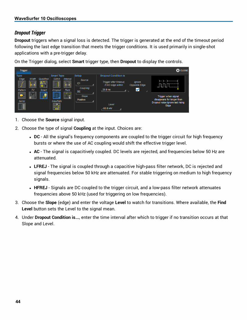
On the Trigger dialog, select Smart trigger type, then Dropout to display the controls.
1. Choose the Source signal input.
2. Choose the type of signal Coupling at the input. Choices are:
l DC - All the signal’s frequency components are coupled to the trigger circuit for high frequencybursts or where the use of AC coupling would shift the effective trigger level.
l AC - The signal is capacitively coupled. DC levels are rejected, and frequencies below 50 Hz areattenuated.
l LFREJ - The signal is coupled through a capacitive high-pass filter network, DC is rejected andsignal frequencies below 50 kHz are attenuated. For stable triggering on medium to high frequencysignals.
l HFREJ - Signals are DC coupled to the trigger circuit, and a low-pass filter network attenuatesfrequencies above 50 kHz (used for triggering on low frequencies).
3. Choose the Slope (edge) and enter the voltage Level to watch for transitions. Where available, the FindLevel button sets the Level to the signal mean.
4. Under Dropout Condition is..., enter the time interval after which to trigger if no transition occurs at thatSlope and Level.
44

Operator's Manual
Runt TriggerRunt triggers when a pulse crosses a first threshold, but fails to cross a second threshold before re-crossingthe first. Other defining conditions for this trigger are the polarity and runt interval (width).
On the Trigger dialog, select Smart trigger type, then choose Runt to display the controls.
1. Choose the Source input.
2. Choose the type of signal Coupling at the input. Choices are:
l DC - All the signal’s frequency components are coupled to the trigger circuit for high frequencybursts or where the use of AC coupling would shift the effective trigger level.
l AC - The signal is capacitively coupled. DC levels are rejected, and frequencies below 50 Hz areattenuated.
l LFREJ - The signal is coupled through a capacitive high-pass filter network, DC is rejected andsignal frequencies below 50 kHz are attenuated. For stable triggering on medium to high frequencysignals.
l HFREJ - Signals are DC coupled to the trigger circuit, and a low-pass filter network attenuatesfrequencies above 50 kHz (used for triggering on low frequencies).
3. Choose the Polarity on which to measure.
4. Enter the voltage crossing Upper Level and Lower Level. Where available, the Find Level button sets thelevels to the positive and negative signal mean.
5. Use Time Condition is settings to create an expression describing the runt interval (width). This conditionis in addition to (AND) the voltage crossing levels. The interval may be:
l Any width Less Than an Upper Interval.
l Any width Greater Than a Lower Interval.
l Any width In Range or Out Range of values. You may describe the range using either:
l Limits, an absolute Upper Interval and Lower Interval.
l Delta, any Nominal width plus or minus a Delta width.
45

WaveSurfer 10 Oscilloscopes
SlewRate TriggerSlewRate triggers when the rising or falling edge of a pulse crosses an upper and a lower level. The pulseedge must cross the thresholds faster or slower than a selected period of time.
On the Trigger dialog, select Smart trigger type, then Slew Rate to display the controls.
1. Choose the Source input.
2. Choose the type of signal Coupling at the input. Choices are:
l DC - All the signal’s frequency components are coupled to the trigger circuit for high frequencybursts or where the use of AC coupling would shift the effective trigger level.
l AC - The signal is capacitively coupled. DC levels are rejected, and frequencies below 50 Hz areattenuated.
l LFREJ - The signal is coupled through a capacitive high-pass filter network, DC is rejected andsignal frequencies below 50 kHz are attenuated. For stable triggering on medium to high frequencysignals.
l HFREJ - Signals are DC coupled to the trigger circuit, and a low-pass filter network attenuatesfrequencies above 50 kHz (used for triggering on low frequencies).
3. Choose the Slope (edge) from which to measure.
4. Enter the voltage crossing Upper Level and Lower Level. Where available, the Find Level button sets thelevel to the positive and negative signal mean.
5. Use Time Condition is settings to create an expression describing the interval within which both levelsmust be crossed. This may be:
l Any time Less Than an Upper Value.
l Any time Greater Than a Lower Value.
l Any time In Range or Out Range of values. You may describe the range using either:
l Limits, an absolute Upper Value and Lower Value.
l Delta, any Nominal width plus or minus a Delta width.
46

Operator's Manual
Trigger HoldoffThe trigger holdoff function is available on WaveSurfer 10 oscilloscopes with the WS10-ADT option installed.
Holdoff is an additional condition that may be set for Edge and Pattern triggers. It can be expressed either asa period of time or an event count. Holdoff disables the trigger temporarily, even if the trigger conditions aremet, until the holdoff conditions are also met. The trigger fires when the holdoff has elapsed.
Use holdoff to obtain a stable trigger for repetitive, composite waveforms. For example, if the number orduration of sub-signals is known, you can disable them by choosing an appropriate holdoff value. Qualifiedtriggers operate using conditions similar to holdoff.
Hold Off by TimeThis is a period of time to wait to fire the trigger, either since the beginning of the acquisition or since thetrigger conditions were met.
Sometimes you can achieve a stable display of complex, repetitive waveforms by placing a holdoff conditionon the time between each successive Edge trigger event. This time would otherwise be limited only by theinput signal, the coupling, and the instrument's bandwidth. Select a positive or negative slope, and aminimum time between triggers.
In the figure below, the bold edges on the trigger source indicate that a positive slope has been selected. Thebroken upward-pointing arrows indicate potential triggers, which would occur if other conditions are met. Thebold arrows indicate where the triggers actually occur when the holdoff time has been exceeded.
Edge trigger with holdoff by time.
Hold Off by EventsFor purposes of Hold Off, Events refers to the number of times the trigger conditions have been met, countedeither from the beginning of the acquisition or since the last trigger. For example, if the hold-off number ofEvents is 2 counted from the beginning of the acquisition, the trigger fires on the third event.
47

WaveSurfer 10 Oscilloscopes
In the figure below, the bold edges on the trigger source indicate that a positive slope has been selected. Thebroken, upward-pointing arrows indicate potential triggers, while the bold ones show where triggers actuallyoccur after the holdoff expires.
Edge trigger with holdoff by events.
Holdoff SettingsTo access the Trigger Holdoff dialog, choose Triggers > Trigger Setup from the menu bar or press the frontpanel Trigger Setup button, then touch the Holdoff tab.
Choose to Holdoff by Time (clock) or Event. None disables Holdoff.
l If using Holdoff by Time, enter the Time in S to wait before triggering.
l If using Holdoff by Events, enter the number of Events to count before triggering.
Choose to Start Holdoff Counter On either:
l Acquisition Start, best for single-shot acquisitions.
l Last Trigger Time, best for acquiring repetitive waveforms.
48

Operator's Manual
DisplayDisplay settings affect the number and style of grids that appear on screen and some of the visualcharacteristics of traces, such as persistence.
By default, the oscilloscope has Auto Grid enabled. This divides the screen into a maximum of three grids,one each for channels/memories, math functions, and zooms. All traces of the same type appear on thesame grid.
To display all types of traces on a single grid, choose Single Grid from the Display dialog.
Two special grid layouts are available: XY Grid, which puts the oscilloscope in XY mode, and XY Single Grid,which creates one XY grid and one single grid for the rest of your traces.
Display SettingsTo access the Display dialogs, choose Display > Display Setup or Display > Persistence Setup.
GridSelect one of the grid types:
Auto, the default, automatically adds or deletes grids as you open or close traces, up to the maximumnumber supported.
Single displays a single grid shared by all traces.
XY displays an XY type trace instead of a traditional voltage/time trace.
XY Single displays a single grid with an XY trace next to it.
To dim or brighten the background grid lines, touch Grid Intensity and enter a value from 0 to 100.
Grid on top superimposes the grid over the waveform.
Check Axis labels to display the voltage values associated with the top and bottom grid lines (calculatedfrom Volts/div) and the time associated with the extreme left and right grid lines (calculated from theTime/div).
TraceChoose a line style for your traces: solid Line or a disconnected series of sample Points.
49

WaveSurfer 10 Oscilloscopes
XYXY displays plot the phase shift between otherwise identical signals. They can be used to display eithervoltage or frequency on both axes, each axis now corresponding to a different signal input, rather than adifferent parameter. The shape of the resulting pattern reveals information about phase difference andfrequency ratio.
NOTE: The inputs can be any combination of channels, math functions, or memories, but both sources musthave the same X-axis scale.
If you choose to display an XY grid, select the source channels to Input X and Input Y.
PersistenceThe Persistence feature retains waveform traces on the display for a set amount of time before allowingthem to gradually "decay," similar to the display of old phosphor screen oscilloscopes. Use Persistence toaccumulate on-screen points from many acquisitions to see your signal change over time. The persistencemodes show the most frequent signal path in three-dimensional intensities of the same color (Analog), orgraded in a spectrum of colors (Color). You can show persistence for any channel, math function, or memory.
Access the Persistence dialog by choosing Display > Persistence Setup. Check Persistence On to shownpersistence, then select the mode, saturation level, persistence time, and last trace display.
Persistence ModeThe Persistence display is generated by repeated sampling of the amplitudes of events over time, and theaccumulation of the sampled data into display maps. These maps create an analog-style display. Statisticalintegrity is preserved because the duration (decay) is proportional to the persistence population for eachamplitude or time combination in the data.
In Analog Mode, as a persistence data map develops, different intensities of thesame color are assigned to the range between a minimum and a maximumpopulation. The maximum population automatically gets the highest intensity, theminimum population gets the lowest intensity, and intermediate populations getintensities in between these extremes. The information in the lower populations (for
50

Operator's Manual
example, down at the noise level) could be of greater interest to you than the rest. The Analog persistenceview highlights the distribution of data so that you can examine it in detail.
Color Mode persistence works on the same principle as Analog persistence, butinstead uses the entire color spectrum to map signal intensity: violet for minimumpopulation, red for maximum population. In this mode, all traces use all colors, whichis helpful for comparing amplitudes by seeking like colors among the traces.
Other Persistence SettingsBesides the different modes, you can select a Saturation level as a percentage of the maximum population.All populations above the saturation population are then assigned the highest color intensity: that is, they aresaturated. At the same time, all populations below the saturation level are assigned the remainingintensities. Data populations are dynamically updated as data from new acquisitions is accumulated. Asaturation level of 100% spreads the intensity variation across the entire distribution; at lower saturationlevels the intensity will saturate (become brighter) at the percentage value specified. Lowering thispercentage causes the pixels to be saturated at a lower population and makes visible those events rarelyseen at higher saturation levels.
Persistence Time is the duration of time (in seconds) after which persistence data is erased from thedisplay.
Choose to superimpose the last waveform over the persistence display by selecting Show Last Trace .
51

WaveSurfer 10 Oscilloscopes
CursorsCursors are markers (lines or cross-hairs) that identify specific voltage and time values on the waveform.Use cursors to make fast, accurate measurements of specific points in the waveform. There are three,standard cursor types available.
Vertical (amplitude) cursor readouts appear the descriptor box for the trace; Horizontal (time) cursorreadouts appear below the Timbebase descriptor box.
Horizontal and vertical cursors.
Cursor Types
Standard CursorsThese cursors can be placed on most any Channel, Memory, Math or Zoom trace.
Horizontal (Time) cursors place vertical lines through a desired point along the horizontal axis.
Vertical (Amplitude) cursors place horizontal lines through a point on the vertical axis.
An option exists to place Horizontal + Vertical cursors together.
Special CursorsSome cursors are offered only in special circumstances. Horizontal (Frequency) cursors look the same asHorizontal (Time) cursors except that they are placed on waveforms that have frequency on the x-axis, suchas FFTs.
In addition, some optional software packages provide cursors and help markers that are specific to theapplication.
52

Operator's Manual
Cursor Settings
Display CursorsTo quickly turn on/off cursors, either:
l From the menu bar, choose Cursors then select the desired cursor type from the drop-down list.
l On the front panel, press the Cursor Type button repeatedly to cycle through all the cursor types. Stopwhen the desired type is displayed.
Position CursorsTe easiest way to position a cursor is to touch and drag the cursor line to a new position.
Alternatively, with the cursor on, turn the front panel Cursors knob. If there is more than one cursor line, pushthe Cursor knob until the correct line is selected, then turn the knob to move it.
Use the Position data entry controls on the Standard Cursors dialog to place cursors precisely.
Standard Cursors DialogThese controls can be used instead of the front panel controls to set cursors or to refine the cursor setup.Access the dialog by choosing Cursors > Cursors Setup from the menu bar.
Cursor Type buttons select the type of cursor displayed on the grid.
The Position controls at the right-side of the Standard Cursors dialog display the current cursor location andcan be used to set a new location. The options available depend on the Cursor Type settings.
l X 1 (negative) and X 2 (positive) time from the zero point.
l Y 1 (negative) and Y 2 (positive) number of divisions from the zero level. May be a fraction of adivision.
l Track locks cursor lines so they move together, maintaining their same relative distance from eachother.
53

WaveSurfer 10 Oscilloscopes
MeasureMeasurement parameters are tools that give you access to a wide range of waveform properties. Use themto analyze many attributes of your waveform such as rise-time, rms voltage, and peak-to-peak voltage.
You can create a custom set of up to six parameters drawn from all the standard measurements, as well asspecialized measurements installed with optional software packages.
Measurement readouts appear in a table below the grid. Readouts can be individually turned on/off. Toquickly access the Measure Setup dialog if it is closed, touch any cell of the readout table.
Measurement readout table open below grid showing statistics and histicons.(Histicons available with the WS10-ADT option.)
Set Up MeasurementsTo configure custom measurements to add to the table of parameter readouts:
1. From the menu bar, choose Measure > Measure Setup.
2. Check Show Table to display the readout on screen.
3. Touch the Measure button next to an unused Px location (or one that you want to change), then choosethe measurement from the pop-up window.
54

Operator's Manual
4. For each input required by the measurement, touch Source and select the waveform to be measured.
5. Optionally, set a measurement gate by entering the Gate Start and Stop divisions or dragging the gateposts from the far left and right edges of the grid to reposition them.
6. Choose to display Statistics or Histicons (WS10-ADT only) on the measurement readout table.
Gating MeasurementsBy using gates, you can narrow the span of the waveform on which to perform parameter measurements,allowing you to focus on the area of greatest interest. For example, if you "gate" five rising edges of thewaveform, the parameter calculations for rise time are performed only on the five pulses bounded by thegate posts.
The default starting positions of the gate posts are 0 div and 10 div, which coincide with the left and rightends of the grid. The gate, therefore, initially encloses the entire waveform.
The quickest way to set a gate is to drag the gate posts located at the far left and right of the grid to thedesired positions. You can refine this setting by specifying a position down to hundredths of a division in theGate Start and Stop fields on the Measure dialog dialog. All parameters share the same gate.
Touch the Default button to return gates to the width of the trace.
Viewing StatisticsYou can add the statistical measures value(last), mean, min., max., sdev, and num(ber of measurementscomputed) to the measurement parameter readout table by checking Statistics On. You can also chooseMeasure > Statistics from the menu bar.
The num statistic is the number of measurements computed. For any parameter that computes on an entirewaveform (like amplitude, mean, minimum, maximum, etc.) the value displayed represents the number ofsweeps.
For any parameter that computes on every event, the value displayed is equal to the number of events peracquired waveform. If x waveforms were acquired, the value represents x times the number of cycles perwaveform. The value(last) statistic is equal to the measurement of the last cycle on the last acquisition.
To reset the statistics counter, touch Clear Sweeps on the display or front panel.
Viewing HisticonsThe histicon capability is available on WaveSurfer 10 oscilloscopes with the WS10-ADT option installed.
Histicons are miniature histograms of measurement parameters that appear on the measurement table.These thumbnail histograms let you see at a glance the statistical distribution of each parameter. Select theHisticons checkbox to turn on histicons.
55

WaveSurfer 10 Oscilloscopes
List of Standard MeasurementsMeasurements included standard with the oscilloscope are listed below alphabetically.
NOTE: There may be additional parameters available depending on the software options installed on theoscilloscope.
Measurement Description
Amplitude(ampl)
Measures the difference between upper and lower levels in two-level signals. Differs from pkpk in that noise,overshoot, undershoot, and ringing do not affect the measurement. Amplitude is calculated by using theformula Top – Base. On signals not having two major levels (such as triangle or saw-tooth waves), theamplitude parameter returns the same value as peak-to-peak.
Area Integral of data: Computes area of the waveform relative to zero level. Values greater than zero contributepositively to the area; values less than zero, negatively.
BaseLower of two most probable states (higher is top). Measures lower level in two-level signals. Differs from min inthat noise, overshoot, undershoot, and ringing do not affect measurement. On signals not having two majorlevels (such as triangle or saw-tooth waves), the amplitude parameter returns the same value as minimum.
DelayTime from trigger to transition: Measures time between trigger and first 50% crossing of specifies signal. Delaycan be used to measure the propagation delay between two signals by triggering on one and determiningdelay of other.
Duty Cycle Percent of period for which data are above or below the 50% level of the signal.
Fall 80-20%(fall8020)
Duration of pulse waveform's falling transition from 80% to 20% of the amplitude averaged for all fallingtransitions between the measurement gates. On signals not having two major levels (triangle or saw-toothwaves, for example), top and base can default to maximum and minimum, giving less predictable results.
Fall time(fall)
Duration of pulse waveform's falling transition from 90% to 10% of the amplitude averaged for all fallingtransitions between the measurement gates. On signals not having two major levels (triangle or saw-toothwaves, for example), top and base can default to maximum and minimum, giving less predictable results.
Frequency(freq)
Period of cyclic signal measured as time between every other pair of 50% crossings. Starting with firsttransition after left measurement gate. The period is measured for each transition pair. The reciprocal of eachperiod measurement is calculated as the frequency.
Maximum(max)
Measures highest point in waveform. Unlike top, does not assume waveform has two levels.
Mean Average of data for time domain waveform. Computed as centroid of distribution for a histogram of the datavalues.
Minimum(min)
Measures the lowest point in a waveform. Unlike base, does not assume waveform has two levels.
None Disables parameter calculation
Overshoot-Amount of overshoot following a falling edge. This is represented as percentage of amplitude. Overshoot- iscalculated using the formula (base - min.)/ampl x 100. On signals not having two major levels (triangle or saw-tooth waves, for example), may not give predictable results.
Overshoot+Amount of overshoot following a rising edge specified This is represented as a percentage of amplitude.Overshoot+ is calculated using the formula (max. - top)/ampl x 100. On signals not having two major levels(triangle or saw-tooth waves, for example), may not give predictable results.
Peak to Peak(pkpk)
Difference between highest and lowest points in waveform. Unlike ampl, does not assume the waveform hastwo levels. Peak to peak is calculated using the formula maximum – minimum.
56

Operator's Manual
Measurement Description
Period The time between every other pair of 50% crossings. Starting with first transition after left measurement gate,period is measured for each transition pair, with values averaged to give final result.
Phase Phase difference between signal analyzed and signal used as reference. Both signals are measured from the50% point of their rising edges.
Rise 20-80%(rise2080)
Duration of pulse waveform's rising transition from 20% to 80% of the amplitude averaged for all risingtransitions between the measurement gates. On signals not having two major levels (triangle or saw-toothwaves, for example), top and base can default to maximum and minimum, giving less predictable results.
Rise TimeDuration of pulse waveform's rising transition from 10% to 90% of the amplitude averaged for all risingtransitions between the measurement gates. On signals not having two major levels (triangle or saw-toothwaves, for example), top and base can default to maximum and minimum, giving less predictable results.
RMSRoot Mean Square of data between the measure gates calculated using the formula:
Where: vi denotes measured sample values, and N = number of data points within the periods found up tomaximum of 100 periods.
Skew Time of clock1 edge minus time of nearest clock2 edge. Both signals are measured from the 50% point of theirrising edges.
Std Dev(sdev)
Standard deviation of the data between the measure gates using the formula:
Where: vi denotes measured sample values, and N = number of data points within the periods found up tomaximum of 100 periods. This is equivalent to the rms for a zero-mean waveform. Also referred to as AC RMS
Top
Higher of two most probable states (base is lower). Measures higher level in two-level signals. Differs frommax in that noise, overshoot, undershoot, and ringing do not affect measurement. On signals not having twomajor levels (such as triangle or saw-tooth waves), the amplitude parameter returns the same value asminimum.
Width
Width of cyclic signal determined by examining 50% crossings in data input. If first transition after left cursor isa rising edge, waveform is considered to consist of positive pulses and width the time between adjacent risingand falling edges. Conversely, if falling edge, pulses are considered negative and width the time betweenadjacent falling and rising edges. For both cases, widths of all waveform pulses are averaged for the finalresult.
WidthN(widn)
Time of cyclic signal determined by examining 50% crossings in data input. The widthN is measured fromfalling edge to rising edge.
57
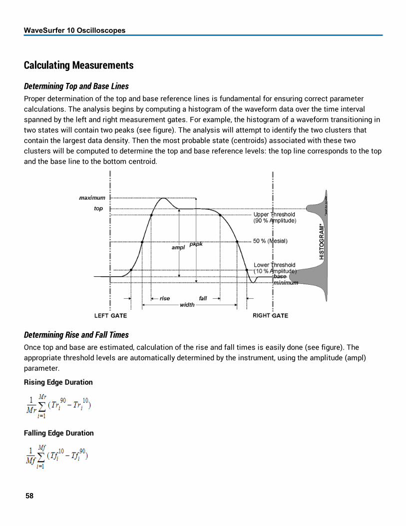
WaveSurfer 10 Oscilloscopes
Calculating Measurements
Determining Top and Base LinesProper determination of the top and base reference lines is fundamental for ensuring correct parametercalculations. The analysis begins by computing a histogram of the waveform data over the time intervalspanned by the left and right measurement gates. For example, the histogram of a waveform transitioning intwo states will contain two peaks (see figure). The analysis will attempt to identify the two clusters thatcontain the largest data density. Then the most probable state (centroids) associated with these twoclusters will be computed to determine the top and base reference levels: the top line corresponds to the topand the base line to the bottom centroid.
Determining Rise and Fall TimesOnce top and base are estimated, calculation of the rise and fall times is easily done (see figure). Theappropriate threshold levels are automatically determined by the instrument, using the amplitude (ampl)parameter.
Rising Edge Duration
Falling Edge Duration
58

Operator's Manual
Where Mr is the number of leading edges found, Mf the number of trailing edges found, the time when
rising edge i crosses the x% level, and the time when falling edge i crosses the x% level.
Determining Time ParametersTime parameter measurements such as width, period and delay are carried out with respect to the mesialreference level, located halfway (50%) between the top and base reference lines.
59

WaveSurfer 10 Oscilloscopes
MathMath traces ) display the result of applying a mathematical operation to a source trace. The output of a mathfunction is always another trace, whereas the output of a measurement parameter is a tabular readout of themeasurement.
Math can be applied to any channel (Cx), zoom (Zx), or memory (Mx) trace. On oscilloscopes with the WS10-ADT option, it can even be applied to another math trace (Fx), allowing you to chain operations (for example,trace F1 can show the average of C1, while trace F2 provides the integral of F1). Functions such as Trendcan be applied to measurement parameters (Px) to plot the history of the measurement.
In addition to the extensive math capabilities that are standard with every oscilloscope, enhanced mathanalysis tools customized for various industries and applications are offered through optional softwarepackages. To learn about math tools available in each optional package, see the datasheets on the TeledyneLeCroy website at teledynelecroy.com. If you have installed software options, these capabilities areaccessed through the oscilloscope Analysis menu, rather than the Math menu, although special measureparameters and math functions will be available when using Measure and Math dialogs.
Single vs. Dual Operator FunctionsSingle functions perform one operation on one or two input sources.
Dual functions chain two operations to arrive at a single result. This saves you the effort of having to chaintwo separate math functions. As with single functions, the number of sources required will vary based on theoperation. You may need only one source for Operator1, but two for Operator2 (the result of the first operationcounts as one source).
60

Operator's Manual
Set Up Math FunctionThis procedure explains how to set up math function (Fx) traces. Function traces take as input one or morechannel, zoom, memory or math traces and output a new math trace.
NOTE: You can set up two, single- or dual-operator math functions on WaveSurfer 10 oscilloscopes with theWS10-ADT option installed. Use the F1 and F2 dialogs to configure the functions; use the Math dialog toenable/disable them.
1. From the menu bar, choose Math > Math Setup.
TIP: If you know which function number you'll be using, select Fx Setup right from the Math menu.
2. If you have the WS10-ADT option installed, choose a location by touching one of the Fx tabs.
3. Choose a single f(x) or dual g(f(x) operator function.
4. In Operator1, choose the math operation to perform.
5. The choice of operator drives the number of Source fields you will see displayed. Make a selection ineach field.
A Summary of the function you are building appears on the dialog. Refer to this to be sure your sourcesare in the proper order to yield the function you want (e.g., C1-C2 vs. C2-C1).
6. If the operator you've selected has any other configurable settings, you'll see a right-hand dialog of thesame name as the operator. Touch the tab to open the dialog and make any further settings. These areexplained on the dialog.
61
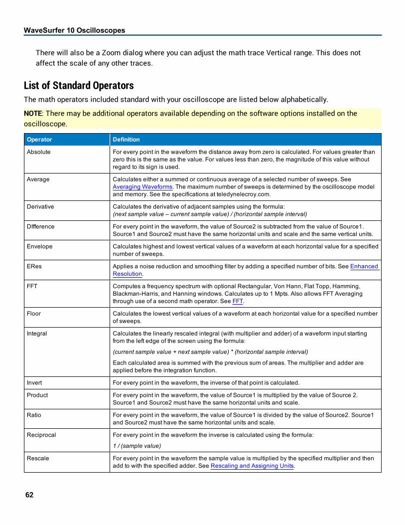
WaveSurfer 10 Oscilloscopes
There will also be a Zoom dialog where you can adjust the math trace Vertical range. This does notaffect the scale of any other traces.
List of Standard OperatorsThe math operators included standard with your oscilloscope are listed below alphabetically.
NOTE: There may be additional operators available depending on the software options installed on theoscilloscope.
Operator Definition
Absolute For every point in the waveform the distance away from zero is calculated. For values greater thanzero this is the same as the value. For values less than zero, the magnitude of this value withoutregard to its sign is used.
Average Calculates either a summed or continuous average of a selected number of sweeps. SeeAveraging Waveforms. The maximum number of sweeps is determined by the oscilloscope modeland memory. See the specifications at teledynelecroy.com.
Derivative Calculates the derivative of adjacent samples using the formula:(next sample value – current sample value) / (horizontal sample interval)
DIfference For every point in the waveform, the value of Source2 is subtracted from the value of Source1.Source1 and Source2 must have the same horizontal units and scale and the same vertical units.
Envelope Calculates highest and lowest vertical values of a waveform at each horizontal value for a specifiednumber of sweeps.
ERes Applies a noise reduction and smoothing filter by adding a specified number of bits. See EnhancedResolution.
FFT Computes a frequency spectrum with optional Rectangular, Von Hann, Flat Topp, Hamming,Blackman-Harris, and Hanning windows. Calculates up to 1 Mpts. Also allows FFT Averagingthrough use of a second math operator. See FFT.
Floor Calculates the lowest vertical values of a waveform at each horizontal value for a specified numberof sweeps.
Integral Calculates the linearly rescaled integral (with multiplier and adder) of a waveform input startingfrom the left edge of the screen using the formula:
(current sample value + next sample value) * (horizontal sample interval)
Each calculated area is summed with the previous sum of areas. The multiplier and adder areapplied before the integration function.
Invert For every point in the waveform, the inverse of that point is calculated.
Product For every point in the waveform, the value of Source1 is multiplied by the value of Source 2.Source1 and Source2 must have the same horizontal units and scale.
Ratio For every point in the waveform, the value of Source1 is divided by the value of Source2. Source1and Source2 must have the same horizontal units and scale.
Reciprocal For every point in the waveform the inverse is calculated using the formula:
1 / (sample value)
Rescale For every point in the waveform the sample value is multiplied by the specified multiplier and thenadd to with the specified adder. See Rescaling and Assigning Units.
62

Operator's Manual
Operator Definition
Roof Calculates the highest vertical values of a waveform at each horizontal value for a specifiednumber of sweeps.
Square For every point in the waveform, the square of the sample value is calculated.
Square Root For every point in the waveform, the square root of the sample value is calculated.
Sum For every point in the waveform, the value of Source1 is added to the value of Source 2.Source1and Source2 must have the same horizontal units and scale and the same vertical units.
Trend Produces a waveform composed of a series of parameter measurements in the order themeasurements were taken. The vertical units are those of the source parameter, the horizontal unitis measurement number. The trend contains a single value for each measurement.
Zoom Produces a magnified trace of a selected portion of the input waveform. See Zooming Traces.
Advanced Debut Toolkit Math FunctionsThese operators are added with the WS10-ADT option.
Operator Definition
Average Calculates either a summed or continuous average of a selected number of sweeps. SeeAveraging Waveforms. The maximum number of sweeps is determined by the oscilloscope modeland memory. See the specifications at teledynelecroy.com.
ERes Applies a noise reduction and smoothing filter by adding a specified number of bits. See EnhancedResolution.
Exp Calculates the antilog to the base e of the source; that is, e raised to the power equal to the source.
Exp10 Same as Exp, using base 10.
Invert For every point in the waveform, the inverse of that point is calculated.
Ln Peforms a natural log of a waveform. Values less than or equal to zero are set to underflow.
Log10 Performs a log base 10 of a waveform. Values less than or equal to zero are set to underflow.
Rescale For every point in the waveform the sample value is multiplied by the specified multiplier and thenadd to with the specified adder. See Rescaling and Assigning Units.
Trend Produces a waveform composed of a series of parameter measurements in the order themeasurements were taken. The vertical units are those of the source parameter, the horizontal unitis measurement number. The trend contains a single value for each measurement. See Trend.
63

WaveSurfer 10 Oscilloscopes
FFTFor a large class of signals, you can gain greater insight by looking at spectral representation rather thantime description. Signals encountered in the frequency response of amplifiers, oscillator phase noise andthose in mechanical vibration analysis, for example, are easier to observe in the frequency domain.
If sampling is done at a rate fast enough to faithfully approximate the original waveform (usually five timesthe highest frequency component in the signal), the resulting discrete data series will uniquely describe theanalog signal. This is of particular value when dealing with transient signals because, unlike FFT,conventional swept spectrum analyzers cannot handle them.
Because of its versatility, FFT analysis has become a popular analysis tool. However, some care must betaken with it. In most instances, incorrect positioning of the signal within the display grid will significantlyalter the spectrum, producing effects such as leakage and aliasing that distort the spectrum.
An effective way to reduce these effects is to maximize the acquisition record length. Record length directlyconditions the effective sampling rate of the oscilloscope and therefore determines the frequency resolutionand span at which spectral analysis can be carried out.
Set Up FFT1. Follow the usual steps to set up a math function, selecting FFT from the Frequency Analysis submenu.
2. Open the FFT right-hand dialog.
3. Choose an Output type.
4. Optionally, choose a weighting Window. See below for more information about FFT weighting windows.
5. Depending on your Output Type selection, you may also make selections for Line Impedence. By default,the FFT function assumes that the oscilloscope is terminated in 50 Ohms. If an external terminator isbeing used, this setting can be changed to properly calculate the FFT based on the new terminationvalue.
6. Check the Suppress DC box to make the DC bin go to zero. Otherwise, leave it unchecked.
64

Operator's Manual
Choosing a WindowThe choice of a spectral window is dictated by the signal's characteristics. Weighting functions control thefilter response shape, and affect noise bandwidth as well as side lobe levels. Ideally, the main lobe should beas narrow and flat as possible to effectively discriminate all spectral components, while all side lobesshould be infinitely attenuated. The window type defines the bandwidth and shape of the equivalent filter tobe used in the FFT processing.
Rectangular windows provide the highest frequency resolution and are useful for estimating the type ofharmonics present in the signal. Because the rectangular window decays as a (sinx)/x function in thespectral domain, slight attenuation will be induced. Functions with less attenuation (Flat Top and Blackman-Harris) provide maximum amplitude at the expense of frequency resolution, whereas Hamming and Von Hannare good for general purpose use with continuous waveforms.
Window Type Applications and Limitations
Rectangular These are normally used when the signal is transient (completely contained in the time-domain window)or known to have a fundamental frequency component that is an integer multiple of the fundamentalfrequency of the window. Signals other than these types will show varying amounts of spectral leakageand scallop loss, which can be corrected by selecting another type of window.
Hanning (Von Hann) These reduce leakage and improve amplitude accuracy. However, frequency resolution is also reduced.
Hamming These reduce leakage and improve amplitude accuracy. However, frequency resolution is also reduced.
Flat Top This window provides excellent amplitude accuracy with moderate reduction of leakage, but with reducedfrequency resolution.
Blackman-Harris It reduces the leakage to a minimum, but with reduced frequency resolution.
FFTWindow Filter Parameters
Window Type Highest Side Lobe (dB) Scallop Loss (dB) ENBW (bins) Coherent Gain (dB)
Rectangular -13 3.92 1.0 0.0
Von Hann -32 1.42 1.5 -6.02
Hamming -43 1.78 1.37 -5.35
Flat Top -44 0.01 3.43 -11.05
Blackman-Harris -67 1.13 1.71 -7.53
65

WaveSurfer 10 Oscilloscopes
Averaging Waveforms
Summed AveragingSummed Averaging is the repeated addition, with equal weight, of successive source waveform records. If astable trigger is available, the resulting average has a random noise component lower than that of a single-shot record. Whenever the maximum number of sweeps is reached, the averaging process stops. In Summedaveraging, you specify the number of acquisitions to be averaged. The averaged data is updated at regularintervals.
An even larger number of records can be accumulated simply by changing the number in the dialog. However,the other parameters must be left unchanged or a new averaging calculation will be started. You can pausethe averaging by changing the trigger mode from NORM/AUTO to STOP. The instrument resumes averagingwhen you change the trigger mode back to NORM/AUTO.
You can reset the accumulated average by pushing the CLEAR SWEEPS button or by changing an acquisitionparameter such as input gain, offset, coupling, trigger condition, timebase, or bandwidth limit. The number ofcurrent averaged waveforms of the function, or its zoom, is shown in the acquisition status dialog. Whensummed averaging is performed, the display is updated at a reduced rate to increase the averaging speed(points and events per second).
Continuous AveragingContinuous Averaging, the default setting, is the repeated addition, with unequal weight, of successivesource waveforms. It is particularly useful for reducing noise on signals that drift very slowly in time oramplitude. The most recently acquired waveform has more weight than all the previously acquired ones: thecontinuous average is dominated by the statistical fluctuations of the most recently acquired waveform. Theweight of ‘old' waveforms in the continuous average tends to zero (following an exponential rule) at a ratethat decreases as the weight increases.
You determine the importance of new data vs. old data by assigning a weighting factor. Continuousaveraging allows you to make adjustments to a system under test and to see the results immediately. Theformula for both summed and continuous averaging is:
new average = (new data + weight * old average)/(weight + 1)
However, by setting a "sweeps" value, you establish a fixed weight that is assigned to the old average oncethe number of "sweeps" is reached. For example, for a sweeps (weight) value of 4:
1st sweep (no old average yet): new average = (new data +0 * old average)/(0 + 1) = new data only
2nd sweep: new average = (new data + 1*old average)/(1 + 1) = 1/2 new data +1/2 old average
3rd sweep: new average = (new data + 2 * old average)/(2 + 1) = 1/3 new data + 2/3 old average
4th sweep: new average = (new data + 3 * old average)/(3 + 1) = 1/4 new data + 3/4 old average
5th sweep: new average = (new data + 4 * old average)/(4 + 1) = 1/5 new data + 4/5 old average
66

Operator's Manual
6th sweep: new average = (new data + 4 * old average)/(4 + 1) = 1/5 new data + 4/5 old average
7th sweep: new average = (new data + 4 * old average)/(4 + 1) = 1/5 new data + 4/5 old average
In this way, for sweeps > 4 the importance of the old average begins to decrease exponentially.
NOTE: The number of sweeps used to compute the average is displayed at the bottom of the trace descriptorbox.
Set Up AveragingTo quickly set up Continuous Averaging (only), access the Channel setup dialog and enter the number ofsweeps to average in Averaging. The valid range is 1 to 1,000,000 sweeps.
To apply Continuous or Summed Averaging as a Math function:
1. Follow the usual steps to set up a math fuction, selecting Average from the Basic Math submenu.
2. On the Average right-hand dialog, choose Summed or Continuous.
3. Touch Sweeps and provide a value. The valid range is 1 to 1,000,000 sweeps.
Enhanced ResolutionERes (Enhanced Resolution) filtering increases vertical resolution, allowing you to distinguish closelyspaced voltage levels. The instrument's ERes function is similar to smoothing the signal with a simple,moving-average filter. However, it is more efficient concerning bandwidth and pass-band filtering.
Use ERes:
l On single-shot acquisitions, or where the data record is slowly repetitive (cases where you cannot useaveraging).
l To reduce noise on noticeably noisy signals when you do not need to perform noise measurements.
l When performing high-precision voltage measurements (e.g., zooming with high vertical gain).
ERes can be applied as a form of Pre-Processing, or as a Math function.
Set Up Enhanced Resolution (ERes)To quickly set up ERes, open the Channel setup dialog and in the Pre-Processing section select a NoiseFilter (ERes) bit size .
To apply ERes as a Math function:
1. Follow the usual steps to set up a math function, selecting ERes from the Filter submenu.
2. Touch the Trace On checkbox.
3. Touch the ERes right-hand dialog tab , then touch bits and make a selection from the pop-up menu.
67

WaveSurfer 10 Oscilloscopes
How the Instrument Enhances ResolutionThe instrument's enhanced resolution feature improves vertical resolution by a fixed amount for each filter.This real increase in resolution occurs whether or not the signal is noisy, or your signal is single-shot orrepetitive. The signal-to-noise ratio (SNR) improvement you gain is dependent on the form of the noise in theoriginal signal. The enhanced resolution filtering decreases the bandwidth of the signal, filtering out some ofthe noise.
The instrument's constant phase finite impulse response (FIR) filters provide fast computation, excellentstep response in 0.5 bit steps, and minimum bandwidth reduction for resolution improvements of between0.5 and 3 bits. Each step corresponds to a bandwidth reduction factor of two, allowing easy control of thebandwidth resolution trade-off. The parameters of the six filters are given in the following table.
Resolution increased by -3 dB Bandwidth(x Nyquist)
Filter Length(Samples)
0.5 0.5 2
1.0 0.241 5
1.5 0.121 10
2.0 0.058 24
2.5 0.029 51
3.0 0.016 117
With low-pass filters, the actual SNR increase obtained in any particular situation depends on the powerspectral density of the noise on the signal.
The improvement in SNR corresponds to the improvement in resolution if the noise in the signal is white(evenly distributed across the frequency spectrum). If the noise power is biased towards high frequencies,the SNR improvement will be better than the resolution improvement.
The opposite may be true if the noise is mostly at lower frequencies. SNR improvement due to the removalof coherent noise signals - feed-through of clock signals, for example - is determined by the fall of thedominant frequency components of the signal in the passband. This is easily ascertained using spectralanalysis. The filters have a precisely constant zero-phase response. This has two benefits. First, the filtersdo not distort the relative position of different events in the waveform, even if the events' frequency contentis different. Second, because the waveforms are stored, the delay normally associated with filtering(between the input and output waveforms) can be exactly compensated during the computation of thefiltered waveform.
The filters have been given exact unity gain at low frequency. Enhanced resolution should therefore notcause overflow if the source data is not overflowed. If part of the source trace were to overflow, filteringwould be allowed, but the results in the vicinity of the overflowed data -- the filter impulse response length -
68

Operator's Manual
would be incorrect. This is because in some circumstances an overflow may be a spike of only one or twosamples, and the energy in this spike may not be enough to significantly affect the results. It would then beundesirable to disallow the whole trace.
Example ERes ApplicationsThe following examples illustrate how you might use the instrument's enhanced resolution function.
Graph Function
In low-pass filtering: The spectrum of a square signal before (left top) and after (leftbottom) enhanced resolution processing. The result clearly illustrates how the filter rejectshigh-frequency components from the signal. The higher the bit enhancement, the lower theresulting bandwidth.
To increase vertical resolution: In the example at left, the lower (inner) trace has beensignificantly enhanced by a three-bit enhanced resolution function.
To reduce noise: The example at left shows enhanced resolution of a noisy signal. Theoriginal trace (left top) has been processed by a 2-bit enhanced resolution filter. The result(left bottom) shows a smooth trace, where most of the noise has been eliminated.
NOTE: While enhanced resolution can only improve the resolution of a trace, it cannot improve the accuracyor linearity of the original quantization. The pass-band causes signal attenuation for signals near the cut-offfrequency. The highest frequencies passed may be slightly attenuated. Perform the filtering on finite record
69

WaveSurfer 10 Oscilloscopes
lengths. Data is lost at the start and end of the waveform and the trace ends up slightly shorter afterfiltering. The number of samples lost is exactly equal to the length of the impulse response of the filter used:between 2 and 117 samples. Normally this loss (just 0.2 % of a 50,000 point trace) is not noticed. However,
you might filter a record so short that no data is output. In that case, however, the instrument would not allowyou to use the ERes feature.
Rescaling and Assigning UnitsThe rescale function allows you to apply a multiplication factor (a) and additive constant (b) to yourwaveform: aX + b. You can do it in the unit of your choice, depending on the type of application.
Set Up Rescaling1. Follow the usual steps to set up a math function, selecting Rescale from the Functions submenu.
2. Touch the Rescale right-hand dialog tab.
3. To apply a multiplication factor:
l Check the First multiply by: box and enter a value for a, the multiplication factor.
l Touch then add: and enter a value for b, the additive constant.
4. To change the output unit of measure from that of the source waveform:
l Check Override units.
l In Output enter the abbreviation for the unit the measure you wish to use.
You can also enter combinations of the unit abbreviations following these rules:
l For the quotient of two units, use the character ":/"
l For the product of two units, use the character "."
l For exponents, append the digit to the unit without a space: S2 = seconds squared.
NOTE: Some units may be converted to simple units (e.g., V.A will display as W).
70

Operator's Manual
Abbreviated Units of Measure
Abbreviation Measure Abbreviation Measure
(blank) No units N Newton
A Ampere OHM Ohm
C Coulomb PAL Pascal
CYCLE Cycles PCT Percent
DB Decibel POISE Poise
DBC Decibel referred to carrier PPM Parts per million
DBM Decibel Milliwatt RAD Radian
DBV Decibel Volts DEG Degree (of arc)
DBUZ Decibel Microamp MNT Minute (of arc)
DEC Decade SAMPLE Sample
DIV Divisions SWEEP Sweeps
Event Events SEC Second (of arc)
F Farad S Second
G Gram SIE Siemens
H Henry T Tesla
HZ Hertz UI Unit interval
J Joule V Volt
K Degree Kelvin VA Volt amps
CEL Degree Celsius W Watt
FAR Degree Fahrenheit WB Weber
L Liter MIN Min
M Meter HOUR Hour
FT Foot DAY Day
IN Inch WEEK Week
YARD Yard
MILE Mile
71

WaveSurfer 10 Oscilloscopes
TrendA Trend is a plot composed of a series of parameter measurements in the order the measurements weretaken. The vertical units are those of the source parameter, the horizontal unit is measurement number. TheTrend contains a single value for each measurement. Trends are especially useful for visualizing the historyof a parameter over an extended period of time or over multiple acquisitions.
1. Follow the usual steps to set up a math function, selecting Trend from the submenu.
2. Open the Trend right-hand dialog.
3. Choose a computation Mode of All (plots multiple points per acquisition) or Average (plots one point peracquisition).
4. To rescale the Trend plot, uncheck Auto Find Scale and enter the new Center and Height/div values. Youcan also use Find Scale to automatically find suitable values.
72

Operator's Manual
MemoryThe oscilloscope is equipped with fourinternal memory slots (Mx) to which you can copy any channel, math,zoom or other special waveform that is active on the grid. This is a convenient way to store an acquisitionfor later viewing and analysis.
Memories are created at the same scale as the source trace, but they can be adjusted independent of theoriginal by using the Zoom controls that appear next to the Mx dialogs.
Save Waveform to Memory1. With the source waveform displayed on the grid, press the front panel Mem button or choose Math >
Memory Setup to open the Memories dialog.
2. Touch the Mx tab corresponding to the memory slot you wish to use.
NOTE: Try to choose an empty slot, as anything currently stored in that location will be overwritten. Allmemories will state if they are empty or an acquisition is stored there.
3. In Copy from Waveform, choose the source trace to copy to memory.
4. Touch Copy Now.
5. Optionally, check Trace On to immediately display the memory. Use the Zoom controls to adjust thescale of the memory while it is turned on.
Save Waveform Files to MemoryTrace (.trc) files saved on other Teledyne LeCroy oscilloscopes can also be stored to internal memory. Usethe Recall Waveform function to save external files to memory. Then, you can use the Memories dialog toenable them from the oscilloscope.
73

WaveSurfer 10 Oscilloscopes
Restore Memory1. Access the Memories dialog by pressing the front panel Mem button or choosing Math > Memory Setup.
2. Check On next to the memory you wish to display. A description of the memory showing the sourcechannel and creation time appears next to each Mx on the dialog.
74

Operator's Manual
AnalysisMost Teledyne LeCroy oscilloscopes calculate measurements for all instances in the acquisition, enablingyou to rapidly and thoroughly analyze a long memory acquisition of thousands or millions of parametervalues, or to apply a variety of mathematical functions to the waveform trace.
WaveScan searches a single acquisition for events that meet specific criteria, enabling you to zoom in onanomalies in the waveform, or scans multiple acquisitions with allowable trigger actions when conditionsare met. It can also be used to filter measurements. A variety of views help you understand the behavior ofwaveforms.
Pass/Fail Testing indicates whether or not waveforms meet a set of defined criteria.
Optional software packages may be purchased that simplify specialized analysis, such as various SerialData Decode options. These add new functionality to the oscilloscope Analysis menu.
WaveScanThe WaveScan® Search and Find tool enables you to search for unusual events in a single capture, or toscan for a particular event in many acquisitions over a long period of time. Each Scan Mode is optimized tofind a different type of event. Results are time stamped, tabulated, and can be selected individually.
WaveScan windowwith different scan "views" turned on.
75

WaveSurfer 10 Oscilloscopes
Customize the presentation by choosing different WaveScan display features, or Scan Views. Optionally, setActions to occur automatically when unusual events are found, such as stopping the acquisition or soundingan alarm.
NOTE: Whenever WaveScan is enabled, the instrument reverts to Real-time sampling mode.
Scan ModesThe scan mode determines the type of search to be performed. Select the Mode along with the Source traceto be searched on the main WaveScan dialog. For each mode, different controls appear on the WaveScandialog, providing additional inputs to the search criteria. Make the appropriate entries in these fields beforestarting the search.
EDGE MODE
Edge Mode is used for detecting the occurrence of edges. Events that meet the threshold level are capturedand tabulated. When the acquisition is stopped, scan filters can be applied to the edges to find specificcharacteristics. Additional settings for Edge Mode are:
l Slope. Choose Pos, Neg, or Both.
l Level is (set in...). Choose Percent or Absolute.
l Percent/Absolute Level. Enter a threshold value as a percentage of Top to Base or voltage level. Amarker displayed over the source trace indicates the level.
NON-MONOTONIC MODE
Non-monotonic Mode looks for edges that cross a threshold more than once between high and low levels. Allevents that meet the criteria of slope, hysteresis, and level are presented in a table and highlighted in thesource trace. The value displayed in the table is the difference of the max. and min. of the non-monotonicity.This can be confirmed with cursors. The hysteresis value is used to eliminate noise. A non-monotonicity isdetected only when its amplitude is greater than the hysteresis. Therefore, when setting a hysteresis level,set a value that is greater than the amplitude of the noise. Additional settings for Non-monotonic Mode are:
l Slope. Choose Pos, Neg, or Both.
l Hysteresis is (set in...). Choose Division, Percent, Absolute.
l Division/Percent/Absolute. Enter the hysteresis level in the units you selected.
l Levels are (set in...). Choose Percent, Absolute, or Pk-Pk%.
l High Level and Low Level. Enter the top and bottom thresholds in the units you selected.
RUNT MODE
Runt Mode looks for pulses that fail to cross a specified threshhold. You can search for positive-going ornegative-going runts, or both. An adjustable hysteresis band is provided to eliminate noise.
76

Operator's Manual
In the case of negative-going runt pulses, the value displayed in the table is the difference (delta) of the highlevel of the signal and the runt amplitude (i.e., where the runt bottoms out). This can be confirmed by placingcursors on the runt pulse and reading the delta Y value in the trace labels. In the case of positive-going runtpulses, the value displayed in the table is the absolute value of the amplitude of the runt pulse. Additionalsettings for Runt Mode are:
l Runt Type. Choose Both, Pos, or Neg.
l Hysteresis. Enter the hysteresis level as a percentage or voltage.
l Low Threshold and High Threshold. Enter the levels as a percentage or voltage.
l Absolute Levels. Check this box to enter levels as absolute voltage instead of percentage.
MEASUREMENT MODE
Measurement Mode is used for applying filters to measurements to find those that meet your definedcriteria, helping to isolate particular events within many samples. Markers appear over the source trace toindicate the location of measurement, while the table displays values for the selected parameter that meetthe criteria. Additional Settings for Measurement Mode are:
l Measurement. Choose the measurement parameter you wish to search.
l Filter Method. Choose the operator that indicates the desired relationship to the Filter Limit. Onlymeasurements that meet this criteria are returned.
l Filter Limit. Enter the value that completes the filter criteria.
Alternatively, you can use the Filter Wizard to create the filter criteria.
BUS PATTERN MODE
Bus Pattern Mode ( only) is used for finding 2- to 16-bit patterns across the digital lines. Additional settingsfor Bus Pattern Mode are:
l Viewing. Choose to enter the pattern as Binary or Hex(adecimal).
l Binary/Hex. Enter the pattern.
l Num. Patterns to detect. Enter a whole number.
Scan ViewsScan Views are different ways to view your WaveScan results. You can choose to display viewssimultaneously or visit them sequentially. Just check the boxes at the bottom of the WaveScan dialog forthose views you wish to display. Uncheck the box to turn off the view.
By default, the Source Trace is displayed in the top grid, with markers indicating points in the trace that meetthe search criteria.
Table view displays a table of measurements relevant to your chosen Search Mode next to the source trace.Times view adds columns to the table showing Start and Stop Times for each event.
77
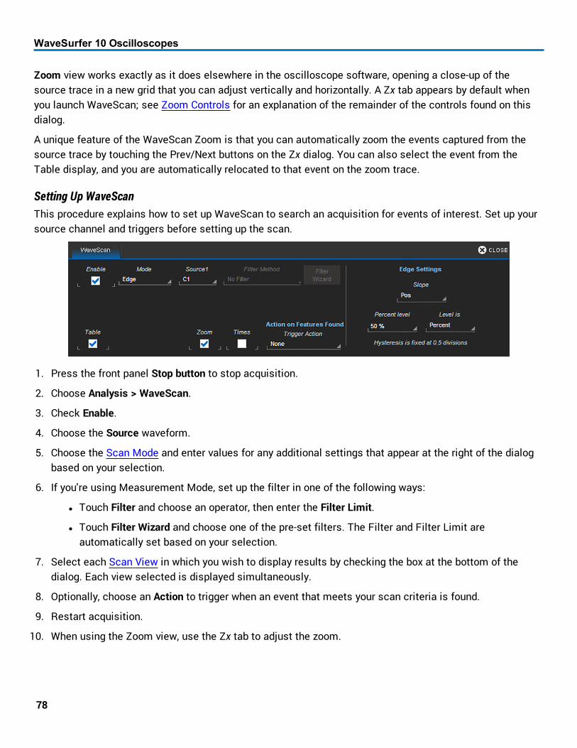
WaveSurfer 10 Oscilloscopes
Zoom view works exactly as it does elsewhere in the oscilloscope software, opening a close-up of thesource trace in a new grid that you can adjust vertically and horizontally. A Zx tab appears by default whenyou launch WaveScan; see Zoom Controls for an explanation of the remainder of the controls found on thisdialog.
A unique feature of the WaveScan Zoom is that you can automatically zoom the events captured from thesource trace by touching the Prev/Next buttons on the Zx dialog. You can also select the event from theTable display, and you are automatically relocated to that event on the zoom trace.
Setting Up WaveScanThis procedure explains how to set up WaveScan to search an acquisition for events of interest. Set up yoursource channel and triggers before setting up the scan.
1. Press the front panel Stop button to stop acquisition.
2. Choose Analysis > WaveScan.
3. Check Enable.
4. Choose the Source waveform.
5. Choose the Scan Mode and enter values for any additional settings that appear at the right of the dialogbased on your selection.
6. If you're using Measurement Mode, set up the filter in one of the following ways:
l Touch Filter and choose an operator, then enter the Filter Limit.
l Touch Filter Wizard and choose one of the pre-set filters. The Filter and Filter Limit areautomatically set based on your selection.
7. Select each Scan View in which you wish to display results by checking the box at the bottom of thedialog. Each view selected is displayed simultaneously.
8. Optionally, choose an Action to trigger when an event that meets your scan criteria is found.
9. Restart acquisition.
10. When using the Zoom view, use the Zx tab to adjust the zoom.
78

Operator's Manual
Pass/Fail TestingPass/Fail testing is a type of mask testing that is particularly useful for comparing newly acquired signals toa previously acquired "golden standard" waveform.
A mask defines an area of the grid against which a source Channel, Zoom, or Math trace is compared. Testconditions are associated with the mask, defining how the waveform is to be compared to the masked area(e.g., some/all values fall within, some/all values fall outside), and a Pass or Fail result is returned indicatingthe condition was found to be true or false.
Mask testing can be done using a pre-defined mask or a mask created from a waveform with user-definedvertical and horizontal tolerances. The mask test can be confined to just a portion of the trace by the use ofa measure gate.
Access Pass/Fail Test DialogsChoose Analysis > Pass/Fail to display the Pass/Fail dialog.
Make MaskUse this procedure to create a new mask based on a live waveform. The mask will cover the area of thewaveform, plus the boundary values you enter.
1. Touch the Make Mask tab to display the dialog.
79

WaveSurfer 10 Oscilloscopes
2. If desired, enter a new Destination File Name and path, or touch Browse and select a previous file tooverwrite. The file name should end with the .msk extension.
3. Touch the Ver Delta and Hor Delta fields and enter boundary values using the pop-up numeric keypad orthe front panel Adjust knob.
4. Touch Make from Trace.
Load MaskUse this procedure in lieu of Make Mask if you have a pre-defined mask file, or wish to recall a mask youpreviously created and saved.
1. Touch the Load Mask tab to display the dialog.
2. To use a saved .msk file, touch File and select the mask.
3. Check View Mask to display the mask over the trace.
Set GatesOptionally, set gates to limit the portion of the waveform that is compared to the mask.
1. Touch More to display the Gate tab, then open the Gate dialog.
2. Enter the Start and Stop horizontal divisions that mark the segment of the waveform to be tested withthis mask. This can be a whole division or a fraction of a division. Divisions are numbered 1-n left toright.
Tip: A quick way to position the gate is to drag the gate posts initially placed at the extreme left and rightends of the grid to the desired points.
80

Operator's Manual
Define Test1. Touch More to display the Test tab, then open the Test dialog.
2. Select one of the conditions that, when True (yes), result in a Pass.
3. Optionally, turn Off/On markers. Markers visually indicate where on the waveform mask violations haveoccurred.
Run Test1. On the main Pass/Fail dialog, select the Source trace to test.
2. Select any additional actions for the oscilloscope to take in the event of a Pass or Fail.
Save the waveform to a file.
Stop the test.
Sound an Alarm.
Send a Pulse via the Aux Out connector.
Capture the screen and process it according to your Hardcopy setting (print, email, or save it to file).
3. Select the Testing checkbox to start the test.
A test counter showing the number of sweeps and the number that Passed or Failed appears below thegrid area. If you have turned on markers, the source waveform samples that Failed the mask test areoverlaid in red on the grid; the samples that Passed the test are overlaid in green.
Removing a Mask from the Display1. Access the Pass Fail dialogs.
2. Touch the Delete Mask button.
81
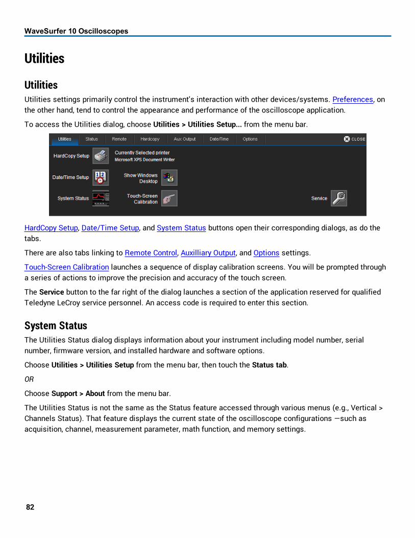
WaveSurfer 10 Oscilloscopes
Utilities
UtilitiesUtilities settings primarily control the instrument's interaction with other devices/systems. Preferences, onthe other hand, tend to control the appearance and performance of the oscilloscope application.
To access the Utilities dialog, choose Utilities > Utilities Setup... from the menu bar.
HardCopy Setup, Date/Time Setup, and System Status buttons open their corresponding dialogs, as do thetabs.
There are also tabs linking to Remote Control, Auxilliary Output, and Options settings.
Touch-Screen Calibration launches a sequence of display calibration screens. You will be prompted througha series of actions to improve the precision and accuracy of the touch screen.
The Service button to the far right of the dialog launches a section of the application reserved for qualifiedTeledyne LeCroy service personnel. An access code is required to enter this section.
System StatusThe Utilities Status dialog displays information about your instrument including model number, serialnumber, firmware version, and installed hardware and software options.
Choose Utilities > Utilities Setup from the menu bar, then touch the Status tab.
OR
Choose Support > About from the menu bar.
The Utilities Status is not the same as the Status feature accessed through various menus (e.g., Vertical >Channels Status). That feature displays the current state of the oscilloscope configurations —such asacquisition, channel, measurement parameter, math function, and memory settings.
82

Operator's Manual
Remote Control SettingsThe Remote dialog contains settings to configure remote control of the instrument. Supported protocols are:
l TCPIP (Ethernet). If you choose this option, also install Teledyne LeCroy's VICP drivers on thecontroller. These are included in the VICP Passport plug-in, available free from teledynelecroy.com.The instrument uses Dynamic Host Configuration Protocol (DHCP) as its default addressing protocol.You can assign a static IP address using the standard Windows network setup menus.
l LXI (Ethernet)
l GPIB. To activate this option, connect the GPIB-USB adapter to any host USB port.
Assign Static IP Address/Name ServerBefore starting, consult with your Network Administrator regaring the oscilloscope's network address,subnet, default gateway.
NOTE: You can also use this procedure to assign a name server if your network uses DHCP addressing.
1. Connect a keyboard to the front panel USB port.
2. From the menu bar, choose Utilities > Utilities Setup, then touch the Remote tab.
3. On the Remote dialog, touch Net Connections.
4. Touch the SMSC icon.
5. On the Ethernet Driver Settings dialog, choose Specify an IP Address.
If assigning a Name server, leave Obtain an IP address via DHCP.
6. Touch the IP Address field, and use the keyboard to enter the address. Repeat for Subnet Mask andDefault Gateway.
Alternatively, touch the Name Server tab and enter the DNS server address.
7. Touch the window close boxes to return to the oscillosocpe application.
83

WaveSurfer 10 Oscilloscopes
Set Up Remote Control1. From the menu bar, choose Utilities > Utilities Setup, then touch the Remote tab.
2. On the Remote dialog, make a Control From selection.
3. If using TCPIP or LXI, touch the Net Connections button and select a network from the pop-up.
4. If using TCPIP and wish to restrict control of the oscilloscope to specific network clients, touch Yes.Enter the IP addresses or DNS names of the authorized controllers in a comma-delimited list.
Configure the Remote Control Assistant Event LogThe Remote Control Assistant monitors communication between the controller and oscilloscope when youare operating the instrument remotely. You can log all events or errors only. The log can be output to anASCII file and is invaluable when you are creating and debugging remote control programs.
1. From the menu bar, choose Utilities > Utilities Setup, then touch the Remote tab.
2. Under Remote Control Assistant, touch Log Mode and choose Off, Errors Only, or Full Dialog.
3. To always clear the log at startup, check Reset to Errors Only and clear at startup.
Export Contents of the Event Log1. From the menu bar, choose Utilities > Utilities Setup, then touch the Remote tab.
2. Touch the Show Remote Control Log button. The Event Logs pop-up is shown.
3. Enter a log file name in DestFilename, or touch Browse and navigate to an existing file.
NOTE: New contents will overwrite the existing content; it is not appended.
4. Touch Export to Text File.
84
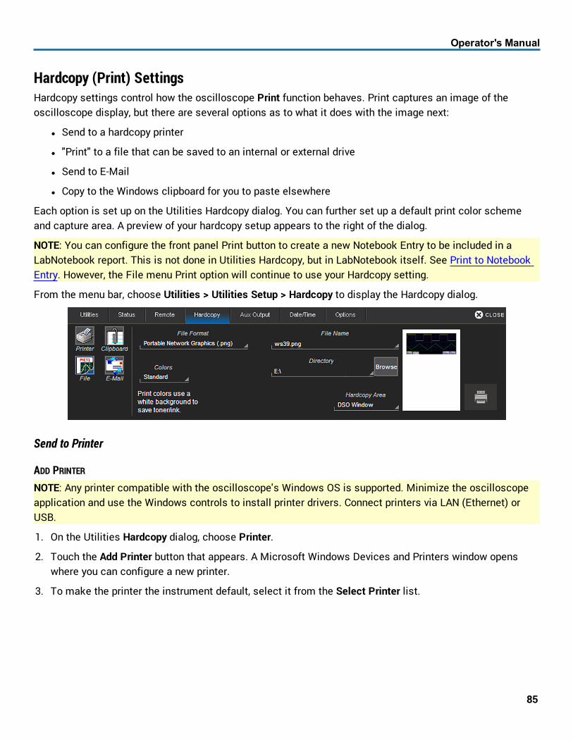
Operator's Manual
Hardcopy (Print) SettingsHardcopy settings control how the oscilloscope Print function behaves. Print captures an image of theoscilloscope display, but there are several options as to what it does with the image next:
l Send to a hardcopy printer
l "Print" to a file that can be saved to an internal or external drive
l Send to E-Mail
l Copy to the Windows clipboard for you to paste elsewhere
Each option is set up on the Utilities Hardcopy dialog. You can further set up a default print color schemeand capture area. A preview of your hardcopy setup appears to the right of the dialog.
NOTE: You can configure the front panel Print button to create a new Notebook Entry to be included in aLabNotebook report. This is not done in Utilities Hardcopy, but in LabNotebook itself. See Print to NotebookEntry. However, the File menu Print option will continue to use your Hardcopy setting.
From the menu bar, choose Utilities > Utilities Setup > Hardcopy to display the Hardcopy dialog.
Send to Printer
ADD PRINTER
NOTE: Any printer compatible with the oscilloscope's Windows OS is supported. Minimize the oscilloscopeapplication and use the Windows controls to install printer drivers. Connect printers via LAN (Ethernet) orUSB.
1. On the Utilities Hardcopy dialog, choose Printer.
2. Touch the Add Printer button that appears. A Microsoft Windows Devices and Printers window openswhere you can configure a new printer.
3. To make the printer the instrument default, select it from the Select Printer list.
85

WaveSurfer 10 Oscilloscopes
PRINT SETUP
1. On the Hardcopy dialog, choose Printer.
2. Touch Select Printer and choose a printer from the list. If you don't see the printer you want, first followsteps to Add Printer.
3. Choose a page Orientation: portrait or landscape.
4. Optionally, choose a color scheme and hardcopy (print) area.
5. Optionally, touch Properties to open the Windows print dialog and adjust printer properties.
Print to FileImage files can be saved to any folder on the oscilloscope hard drive, or to an external drive connected to aUSB port.
1. On the Hardcopy dialog, choose File.
2. Choose the output File Format.
3. Enter a File Name. This will form the basis of all print filenames, until you change it.
NOTE: Numbers at the end of the filename will be truncated, as the instrument appends numbers to thisname with each new file. If you wish to add your own identifying numbers, place them at the front of thename.
4. Optionally, enter the path to a new save Directory, or touch the Browse button and navigate to the folder.
NOTE: The default print folder is C:\...\XStream\Hardcopy. Other types of files that may be saved usingother oscilloscope functions, such as masks and scripts, have their own XStream subfolders.
5. Optionally, choose a color scheme and hardcopy (print) area.
Copy to ClipboardThis procedure copies the screen to the clipboard so you can paste it into another application (MicrosoftWord, for example).
1. On the Hardcopy dialog, choose Clipboard.
2. Optionally, choose a color scheme and hardcopy (print) area.
86

Operator's Manual
Send to E-MailFollow this procedure to e-mail capture files to a preset address. The e-mail connection is set up in Utilities> Preferences Setup > E-Mail.
1. On the Hardcopy dialog, choose E-Mail.
2. Choose the output File Format.
3. If you wish to be able to include messages with the files as they are sent, check Prompt for message tosend with mail.
4. Optionally, choose a color scheme and hardcopy (print) area.
5. To go on and set up the e-mail connection, touch Configure E-Mail Server and recipient.
Choose Print Color SchemeTo change the color of your print output, touch the Color button on the Hardcopy dialog and choose from:
l Standard(default) - prints objects on a black background, as they appear on the display.
l Print - prints objects on a white background using your chosen colors. This option saves ink.
l Black & White - prints objects in grayscale.
Set Print AreaTo limit which part of the touch screen is captured, touch Hardcopy Area on the Hardcopy dialog and choosefrom:
l Grid Area Only - omits dialogs and menus and prints only the grids.
l DSO Window - prints the dialogs with the grids.
l Full Screen - prints the entire touch screen.
87

WaveSurfer 10 Oscilloscopes
Auxiliary Output SettingsUse the Aux Output dialog to configure the output of the Aux Out and Cal Out ports.
Use the Aux Output dialog to configure the output of the Aux Out port. The port outputs a 1.0 V TTL pulsefollowing the selected event.
l Trigger Enabled sends a pulse when the oscilloscope trigger is ready (Ready indicator lit), but notnecessarily fired. It can be used as a gating function to trigger another instrument when theoscilloscope is ready.
l Trigger Out sends a pulse when the oscilloscope trigger fires (Trig'd Indicator lit). It can be used totrigger an external oscilloscope off the instrument's state.
l Pass/Fail generates a pulse when Pass/Fail testing is active and conditions are met. With thisselection, a Pulse Duration data entry control appears. Provide a value within your instrument'sspecified range, which varies by model. Refer to datasheet specifications at teledynelecroy.com.
Off disables auxiliary input/output.
88

Operator's Manual
Date/Time SettingsDate/Time settings control the oscilloscope's timestamp. These numbers appear in the oscilloscopemessage bar and on tables/records internal to the oscilloscope application, such as History Mode andWaveScan.
NOTE: This is not the same as the Timebase reference clock used to synchronize traces.
To access the Date/Time dialog, choose Utilities > Utilities Setup from the menu bar, then touch theDate/Time tab.
Manual MethodEnter the Hour, Minute, Second, Day, Month, and Year, then touch the Validate Changes button.
Internet MethodThis method uses the Simple Network Time Protocol (SNTP) to read the time from time-a.nist.gov. Theoscilloscope must be connected to an internet access device through the LAN (Ethernet) port on yourinstrument's I/O panel. .
If your connection is active, touch the Set from Internet button.
Windows MethodTo set date and time using the internal Windows system clock, touch the Windows Date/Time button. Thisdisplays the standard Windows DateTime Properties pop-up dialog, where you can further configure thesesettings. If you are satisfied with the setup, just touch OK.
OptionsThe Options dialog is used to add or remove software options. This dialog also displays the ScopeID andSerial #. See Adding an Option Key for instructions on using this dialog.
89

WaveSurfer 10 Oscilloscopes
Disk UtilitiesUse the Disk Utilities dialog to manage files and folders on your instrument's hard drive. Disk Spaceinformation is shown at the far right of the dialog for convenience.
NOTE: These tasks can also be accomplished using the standard Microsoft Windows file management tools.Choose File > Minimize to access the Windows desktop and task bar.
Access the Disk Utilities dialog by selecting Utilities > Disk Utilities from the menu bar, or choose any of theSave/Recall functions and open the Disk Utilities tab.
Delete a Single File1. Touch the Delete button.
2. Browse to the current folder containing the file.
3. Browse to the file to be deleted, or use the Upand Down arrow buttons to scroll through the files in thefolder.
4. With the desired file selected, touch Delete File.
Delete All Files in a Folder1. Touch the Delete button.
2. Browse to the current folder containing the file.
3. With the desired folder selected, touch Empty Folder.
Create a New Folder1. Touch Create.
2. Touch Current folder and provide the full path to the new folder, including the folder name.
3. Touch Create Folder.
90

Operator's Manual
Preferences SettingsPreference settings have mostly to do with the appearance and performance of the oscilloscope itself, ratherthan the oscilloscope's interaction with other devices/systems.
Access the Preferences dialog by choosing Utilities > Preference Setup... from the menu bar.
Audible Feedback controls the instrument's audio output. Select this box to hear a beep each time you toucha screen or front panel control.
Automatic Calibration enables or disables the temperature dependent calibration feature. When enabled, theinstrument will offer you a choice of calibrations to perform whenever there is a significant change inambient temperature.
NOTE: If you do not enable this option, the oscilloscope re-calibrates only at startup and whenever youchange certain operating conditions.
Language sets the language used on the display.
There are also tabs linking to Acquisition, E-Mail, and Miscellaneous settings.
91
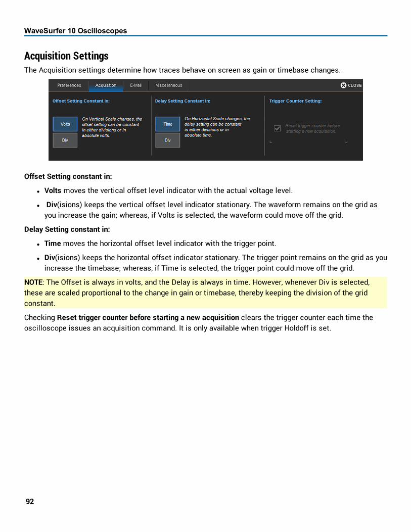
WaveSurfer 10 Oscilloscopes
Acquisition SettingsThe Acquisition settings determine how traces behave on screen as gain or timebase changes.
Offset Setting constant in:
l Volts moves the vertical offset level indicator with the actual voltage level.
l Div(isions) keeps the vertical offset level indicator stationary. The waveform remains on the grid asyou increase the gain; whereas, if Volts is selected, the waveform could move off the grid.
Delay Setting constant in:
l Time moves the horizontal offset level indicator with the trigger point.
l Div(isions) keeps the horizontal offset indicator stationary. The trigger point remains on the grid as youincrease the timebase; whereas, if Time is selected, the trigger point could move off the grid.
NOTE: The Offset is always in volts, and the Delay is always in time. However, whenever Div is selected,these are scaled proportional to the change in gain or timebase, thereby keeping the division of the gridconstant.
Checking Reset trigger counter before starting a new acquisition clears the trigger counter each time theoscilloscope issues an acquisition command. It is only available when trigger Holdoff is set.
92

Operator's Manual
E-MailUse the E-mail dialog to set up e-mail on the oscilloscope.
1. Under E-Mail Server, select the protocol used by your network:
l MAPI (Messaging Application Programming Interface) is the Microsoft interface specification thatallows different messaging and workgroup applications (including e-mail, voice mail, and fax) towork through a single client, such as the Exchange client. MAPI uses the default Windows e-mailapplication.
l SMTP (Simple Mail Transfer Protocol) is a TCP/IP protocol for sending messages from onecomputer to another through a network. This protocol is used on the Internet to route e-mail. Inmany cases no account is needed.
2. Under Configuration:
l If you chose SMTP, touch SMTP Server and enter the network address of your mail server.
l Touch Originator Address (From:) and enter the instrument's e-mail address.
l Touch Default Recipient Address (To:) and enter the recipient's e-mail address.
3. Touch Send Test Mail to send a confirmation message to ensure proper e-mail configuration.
93

WaveSurfer 10 Oscilloscopes
Miscellaneous SettingsThese other Preference settings are located on the Miscellaneous dialog.
To add the Teledyne LeCroy logo to print output, check Print Teledyne LeCroy Logo When Printing Grid AreaOnly. This identifies the instrument as the source of the image.
You can adjust zoom behavior as follows:
l Dimming darkens/shades those areas of the source waveform that are not part of the Zoom trace.
l Control Sensitivity adjusts the sensitivity of the front panel knobs. Optimized applies an accelerationalgorithm to the knobs. Legacy detects rotation of the front panel knobs in a manner similar to ourlegacy oscilloscopes.
Serial Decode Annotation Position: If you have Serial Trigger or Decode options installed on youroscilloscope, this control determines the placement of annotation labels relative to the trace line. It does notappear if there are no installed options.
l On Trace places the label close to the line.
l On Noisy Trace sets the label further from the line to accommodate potential noise spikes in the trace.
Check Enable HTTP Screen Capture to enable remote capture of the oscilloscope display over a netowrk.This setting is required to use the oscilloscope with the WaveStudio software.
94

Operator's Manual
Save/RecallThe oscilloscope File menu allows you to save or retrieve waveform files, measurement table data, andinstrument setup panels.
Access these functions by choosing any of the Save or Recall options from the File menu. The dialogcontains a tab for each file function.
Save/Recall SetupsSave Setups allows you to quickly save up-to-six oscilloscope panel settings to internal storage, while RecallSetups restores them with a touch.
If desired, you can also save oscilloscope panel settings as an .lss file in a different location, such as a USBdrive, and recall them from the same.
Saving Oscilloscope SetupsChoose File > Save Setup... from the menu bar.
SAVE SETUP TO MEMORY
1. Touch one of the Setup data entry controls and enter a name for the memory.
2. Touch the corresponding Save button directly to the left of the Setup field.
The save date/time is displayed above the Setup data entry control.
SAVE SETUP TO FILE1. In Save Panel to File, touch Browse and navigate to the desired folder.
2. Enter a File name, or choose a existing file to overwrite. Touch OK.
3. On the Save Setups dialog, touch Save Now!
95

WaveSurfer 10 Oscilloscopes
Recalling Oscilloscope SetupsChoose File > Recall Setup... from the menu bar.
RECALL SETUP FROM MEMORY
Touch one of the six Recall buttons under Recall From Internal Setup....
NOTE: If a setup has been stored to a location, it is labeled with the save date/time. Otherwise, the slot islabeled Empty.
RECALL SETUP FROM FILE1. In Recall panel from file, touch Browse and navigate to the desired folder.
2. Select the setup file and touch OK.
3. On the Recall Setups dialog, touch Recall Now!
96

Operator's Manual
Save/Recall WaveformsThe Save Waveform function saves trace data to either an internal memory location, or to a text or binaryformat file (.trc). The source waveform can be any trace; for example, a channel, math function, or awaveform stored in another memory.
By default, trace files are saved to the , although you can choose another location, such as a USB drive. Thefile name is autogenerated from the <source trace><trace title><number in sequence> (e.g., C1test000001).
Use Recall Waveform to restore these previously saved waveforms to the display.
NOTE: Only .trc files saved in binary format can be recalled into the oscilloscope.
Save WaveformChoose File > Save Waveform from the menu bar.
NOTE: This dialog is for saving waveforms. Save S-parameter files using the Result Actions Dialog.
SAVE WAVEFORM TO MEMORY
1. Touch Memory.
NOTE: When Memory is selected, only Source and Destination controls are shown on the Save Waveformdialog. When File is selected, many more controls are available.
2. Choose the Source trace you are saving.
3. Choose the Destination location.
4. Touch Save Now!
SAVE WAVEFORM TO FILE1. Touch File.
2. Choose the Source waveform.
3. Optionally, touch Trace Title to change the root file name of your waveforms.
CAUTION. Numbers at the end of this name are truncated because the instrument appends a
97

WaveSurfer 10 Oscilloscopes
number to each file. Place numbers at the beginning, or place an alpha character after thenumber (e.g., XYZ32a).
4. Touch Data Format and select a file format:
l Binary, Teledyne LeCroy's binary file format (.trc). Binary results in the smallest possible file size,and is necessary for recalling waveforms to Teledyne LeCroy instruments.
NOTE: Binary files can be converted to ASCII using Teledye LeCroy utilities such as ScopeExploreror WaveStudio.
l ASCII text file (.txt extension).
l MATLAB text file (.dat extension).
l Excel text file (.csv extension).
l MathCad text file (.prn extension).
l Audio .wav file.
5. Depending on your file format selection, you may also need to specify a SubFormat:
l Word (Binary) represents samples in the output file with 16 bits. Always use this options unlessByte mode is "pre."
l Byte (Binary) represents samples in the output file with 8 bits. This option can result in a loss ofoutput file resolution.
l Auto (Binary) looks at the data and automatically selects either Word or Byte subformat.
l Amplitude only (Text) includes amplitude data for each sample, but not time data.
l Time and Amplitude (Text) includes both types of data for each sample.
l With Header (Text) includes a file header with scaling information.
6. If you selected ASCII format, also touch Delimiter and select a delimiter character from the pop-up menu.
7. In Save Files in Directory, touch Browse and navigate to the desired location. Touch OK.
NOTE: If the oscilloscope is networked, you can touch on Save Files in Directory and enter the fullWindows network address of another location in which to save the file. The oscilloscope must haveaccess to this directory.
8. On the Save Waveform dialog, touch Save Now!
98

Operator's Manual
Recall WaveformChoose File > Recall Waveform from the menu bar.
NOTE: Only .trc files saved in binary format can be recalled into the oscilloscope.
RECALL WAVEFORM FROM MEMORY
1. Touch Memory.
2. Touch Source and choose a memory location from the Select Source pop-up.
3. Touch Destination and select a location into which to open the recalled memory.
4. Mark Show on Recall to display the trace on the grid.
5. Touch Recall Now!
RECALL WAVEFORM FROM FILE1. Touch File.
2. Touch Recall files from directory and enter the path to the waveform folder, or touch Browse and navigateto the folder.
3. Use the Up /Down Arrows to cycle through the available files until the desired file is selected.
Optionally, touch Show only files to apply a search filter (channels, math functions, or memory) to the listof available files.
4. Mark Show on Recall to display the trace on the grid.
5. Touch Recall Now!
99

WaveSurfer 10 Oscilloscopes
Save Table DataThe Save Table function saves tabular measurement data displayed on screen to an Excel or ASCII file. Bydefault, files are saved , although you can choose .
Access the Save Table dialog by choosing File > Save Table from the menu bar.
1. Leave the default Source selection All Displayed.
2. Optionally touch Table Title and enter a new root file name.
CAUTION. Numbers at the end of this name are truncated because the instrument appends anumber to each file. Place numbers at the beginning, or place an alpha character after thenumber (e.g., XYZ32a).
3. Touch Data Format and choose from ASCII (.txt) or Excel (.csv) format.
4. If you selected ASCII format, also touch Delimiter and choose a character.
5. In Save Files in Directory, touch Browse and navigate to the desired folder. Select it and touch OK.
NOTE: If the oscilloscope is networked, you can touch on Save Files in Directory and enter the fullWindows network address of another location in which to save the file. The oscilloscope must haveaccess to this directory.
6. On the Save Table dialog, touch Save Now!
100

Operator's Manual
LabNotebookTeledyne LeCroy's LabNotebook feature extends the documentation capabilities of your oscilloscope. Itallows you to create and save Notebook Entries containing all displayed waveforms, the oscilloscope setupunder which they were taken, and custom annotations.
Notebook Entries are stored in an internal database and are available for recall at any time. Besides storingthe waveform data, LabNotebook also stores your panel setups and parameter measurements. You can backup this database to external media for indefinite storage of waveform data.
The Flashback Recall feature instantly recalls the setups stored with individual Notebook Entries, enablingyou to restore the exact state of the oscilloscope at a later date to perform additional analysis.
Create Notebook EntryA Notebook Entry is a snapshot of the oscilloscope at the moment it is taken: it captures the waveforms,their setups, and any measurements in process. As each new entry is created, it is added to the database ofMy Notebook Entries accessible from the LabNotebook dialog, where they can be recalled to the screenthrough Flashback Recall.
1. Choose File > LabNotebook to open the LabNotebook dialog.
2. Touch Create.
3. Optionally, Enter Report Title and Description.
The default title is the date and time stamp. You can leave this as is, append some descriptive text to it,or completely remove it from your title.
NOTE: By default, you will be prompted to title and annotate notebook entries as they are created. Youcan configure LabNotebook preferences so that these steps are skipped in order to streamline thecreation process. To update entries at a later time, select the entry from the list of Notebook Entries,then open the tab of the same name that appears behind the LabNotebook dialog.
4. Touch Save.
5. Use the Drawing toolbar to annotate the Notebook Entry. Click Done when finished.
101

WaveSurfer 10 Oscilloscopes
LabNotebook Drawing ToolbarThe basic Notebook Entry is a screen capture of the display showing the grids as they were at the time itwas taken. When an entry is first captured, it is immediately displayed in the Drawing window for you toannotate.
A variety of markup tools are available from the toolbar along the top of the window. To use any tool, touchthe icon, then touch the point on the image where you wish to draw or add text.
From left to right, the tools are:
Pen Tool enables you to draw in freehand. Maintain contact with the screen to make a continuous mark.Once you release, you can touch-and-drag the object to any point on the image.
Circle Tool draws a circle around a waveform feature that you want to emphasize. Touch-and-drag acrossthe diameter of the circle. When you release, the circle is placed. You can drag the circle to any location onthe image.
Arrow Tool draws lines with arrowheads for placing callouts. You can rotate these lines through 360 degreesor drag them to any location on the image.
Text Tool opens a textbox for placing labels/annotations on the image. Touch the point on the image to placethe label, then enter the text in the pop-up dialog. Once placed, you can resize the textbox or drag it to anylocation on the image.
Red, Green, and Blue Color Selectors let you quickly change the markup color. Just touch the icon, thenchoose the next drawing tool.
To use additional colors, touch the More Button. This activates a Custom color field. The default customcolor is Yellow. To choose another, touch the color swatch, then select from the Color dialog (the standardWindows Palette dialog). You can enter RGB values, or choose from the spectrum. After saving, the newcolor appears in the Custom field. This remains the markup color until you choose another.
Erase Buttons allow you to remove all or selected drawing objects. Erase All will also undo any Custom colorselection.
Undo Button cancels the last action. Use it to restore any objects you inadvertently erased.
Move Toolbar Button undocks the drawing toolbar so you can move it anywhere on the display. This helps tokeep tools handy when working on a particular area of a waveform. Touch the button again to restore thetoolbar to the top of the Drawing window.
Done Button saves the annotations with the image and closes the Drawing window.
102

Operator's Manual
Manage Notebook EntriesThe LabNotebook dialog is the principal notebook management tool where you can filter, select, view, edit,print, email, save, export/import, or recall Notebook Entries created in the course of your work.
To access the LabNotebook dialog, choose File > LabNotebook from the menu bar.
NOTE: If an external monitor is connected, LabNotebook automatically opens on the external monitor.
Select Notebook EntriesYou must select Notebook Entries before any further action can be performed.
1. Select the notebook from the My Notebooks list.
2. Use the Up and Down arrows to scroll the My Notebook Entries list. The selected entry is highlighted inblue.
OR
To select multiple entries, first check Multi-selection, then Select All or scroll the list touching Select asa desired entry is highlighted. A white arrow appears next to each selected entry.
3. To remove selections from the list, highlight them again and touch Clear, or just touch Clear All.
Filter Notebook EntriesIf there are a large number of notebook entries, you can apply filters to the list before selecting.
1. Select the notebook from the My Notebooks list.
2. Touch the Filter button.
3. On the Filter Entries pop-up, enter the filter criteria. You can use Day/Month/Year, a Keyword, or acombination.
4. Touch Find Now to filter.
5. To restore the full list, touch Clear Filter.
View Notebook EntriesView allows you to preview the selected entries in the report format before printing/saving.
103

WaveSurfer 10 Oscilloscopes
Select the desired entries and touch the View button. Use the scrollbar that appears on the LabNotebookwindow to navigate the report.
Edit Notebook Entries1. Select the notebook from the My Notebooks list.
2. Select the entry from the My Notebook Entries list.
3. Go to the second tab labeled with the entry name.
4. Modify the Title or Description.
5. To add markup to the entry, touch the Scribble button and use the Drawing Toolbar.
Email Notebook EntriesChoose E-Mail to send selected Notebook Entries to the default address specified in the oscilloscopePreferences. To use the E-Mail button, the instrument must have an active network connection and you mustfirst configure the email address and server.
If you have not yet configured email, or if you wish to change the recipient address before sending, open theLabNotebook Preferences tab, then touch the Configure E-Mail button.
Also select whether or not to Attach Setup & Waveform files to the email with the LabNotebook files.
Print Notebook EntriesTo print multiple entries, select them on the main LabNotebook dialog, then touch the Print button on thesame dialog.
To print a single entry, select it on the main LabNotebook dialog, then go to the second tab and touch thePrint button.
Delete Notebook EntriesUse the Delete button to remove selected Notebook Entries, or Delete All to clear the entire My NotebookEntries.
NOTE: Unless you have previously backed up the notebook, deleted entries cannot be restored.
104

Operator's Manual
Create ReportCreate Reports collates the selected Notebook Entries into a single .RTF/.PDF document or HTML archiveusing the report template selected on the LabNotebook Preferences tab. This can be one of the preformattedtemplates or a custom format. It is not necessary to first create a report document to view, email, or printselected Notebook Entries.
1. Select the notebook from the My Notebooks list.
2. Select the entries from the My Notebook Entries list.
3. Choose the output Format.
4. Touch Create Report.
5. On the Create Report window, select the folder in which to save the report.
TIP: Touch Open Explorer Here and use the Windows Explorer to create a new folder. After closing theExplorer, touch the Refresh button to display the folder in the Create Report window.
6. Enter a File name for the report and click OK.
Print to Notebook EntryThe front panel Print button can be configured to capture the display and create a new Notebook Entry. Thisis a convenient way to create new Notebook Entries as you work.
To configure the Print button for Notebook Entries, go to File > LabNotebook > Preferences tab and checkCreate Entry when Hardcopy Pressed.
Flashback RecallOnce a Notebook Entry is made, you can recall it at any time using Flashback Recall. The recall includeswaveforms and oscilloscope settings, so you can analyze the inputs that resulted in that capture.
1. Choose File > LabNotebook to open the LabNotebook dialog.
2. Select the Notebook and Notebook Entry from the lists.
3. Touch the Flashback Recall button.
4. To exit Flashback Recall, touch the Undo button at the far right of the menu bar.
Some result data not included in Flashback Recall are:
l Persistence data (although it is saved in with the Notebook Entry and appears on reports).
l Floating point waveforms resulting from certain math operations that have much higher resolution than16-bits. This extra resolution is not preserved when traces are recalled using Flashback.
l Cumulative Measurements in process when Flashback Recall is entered. When Flashback is used,they lose their history and show instead only the results from the stored waveforms, not including anydata taken from interim acquisitions.
105

WaveSurfer 10 Oscilloscopes
Manage NotebooksLabNotebook stores Notebook Entries in a .zip archive on the instrument hard drive. Each .zip file is oneNotebook comprised of everything shown in the My Notebook Entries list. New Notebooks can be created fordifferent individuals or projects, or an existing Notebook backed up for storage.
NOTE: The default Notebook is D:\Xport\MyLabNotebook.zip. If you've already created Notebook Entries thatyou wish to keep, you can use the backup feature to save them under a new file name or location beforestarting a new Notebook.
Create New Notebook1. Choose File > LabNotebook.
2. Open the Advanced dialog and choose Start New.
3. Enter a File Name for the new Notebook (optionally, choose a new storage folder, as well). Touch OK.
The new notebook now appearsin the Database field on the Advanced dialog. New Notebook Entries will beadded to this file whenever it is selected as the Database.
Back Up Notebook1. Choose File > LabNotebook.
2. Open the Advanced dialog and choose Backup.
3. Optionally, enter a new File Name or choose a new storage Folder.
NOTE: The default is the current notebook name with the extension *.bak.zip appended to it. You canchange this to anything you like, although it is recommended to leave the .zip file extension.
4. Choose to Backup to Removable Disk (this option is active if you have a USB drive attached to theoscilloscope) or Backup to Folder on hard drive.
Import NotebookArchived notebooks can be imported into LabNotebook. This notebook can not be selected as the workingDatabase on the Advanced dialog, and the entries in it are appended to the My Notebook Entries list forselection.
1. Choose File > LabNotebook.
2. Open the Advanced dialog and touch Import From.
3. Navigate to the desired archive and select it. Touch OK.
Delete NotebookUse the standard Windows controls to browse to the notebook in the D:\Xport folder on the oscilloscope harddrive and delete it.
106

Operator's Manual
Customize ReportsThe Advanced tab allows you to customize the report creation function.
Change DirectoriesTo change where Notebooks are stored, change the Notebooks Directory folder.
To change where reports are output, change the Report Directory folder. You can choose an external location,such as a USB drive.
Change Report TemplateDeselect Use Default next to the Template field, then touch Browse and select a different template from theD:\Xport folder.
You can create your own report template and place it in this directory for selection. Templates must besaved as .xsl or .xslt files.
Change LogoThe included LabNotebook report templates use our logo as a placeholder. You can replace this with yourcustom logo. Logo files should be in bitmap (.bmp) format and not exceed 100 pixels high by 180 pixels wide.
1. Copy the logo file to the D:\Xport folder.
2. Choose File > LabNotebook, then touch the Advanced tab.
3. Deselect the Use Default checkbox next to the Logo field.
4. Touch the Browse button and navigate to the the new logo file. Select and touch OK.The new file pathappears in the Logo field with a preview of the image above it.
107

WaveSurfer 10 Oscilloscopes
Configure LabNotebook PreferencesTo configure the behavior of the LabNotebook tool, on the menu bar, choose File > Lab Notebook, then touchthe Preferences tab.
Select/deselect the following options:
Prompt for Entry Title Before Saving opens the LabNotebook dialog when a new entry is created. You canelect to name notebook entries using only the date/timestamp by leaving this box unchecked.
Annotate Entry Before Saving opens the Drawing Toolbar to annotate a notebook entry as soon as it iscreated.
Create Entry When Hardcopy Pressed configures the front panel print button to create a new notebook entrywhenever it is pressed.
Use Print Colors outputs waveforms on a white background. This option helps save ink/toner when printing.
Hardcopy Area determines how much of the screen image is included in the report: grid area only, grid areaplus dialog, whole screen. Touch the field and choose from the pop-up menu.
Attach Setup & Waveforms attaches these files for each trace in the report: waveform data (.trc), a screendump (.png), oscilloscope setup file (.lss), report template file (.xsl), and export record (.htm).
Optionally, touch the Configure E-Mail button to set the recipient address and server information on thePreferences E-mail dialog.
108

Operator's Manual
Maintenance
CleaningClean only the exterior of the instrument using a soft cloth moistened with water or an alcohol solution. Donot use harsh chemicals or abrasive elements. Under no circumstances submerge the instrument or allowmoisture to penetrate it. Avoid electric shock by unplugging the power cord from the AC outlet beforecleaning.
CAUTION. Do not attempt to clean internal parts. Refer to qualified service personnel.
CalibrationThe oscilloscope is calibrated at the factory prior to being shipped. This calibration is run at 23° C (± 2° C)and is valid for temperatures ± 5° C of the original calibration temperature. Within this temperature range theoscilloscope will meet all of the specifications.
The oscilloscope will offer you two calibration options whenever the temperature ranges outside this limit:
l Calibrate Allpossible combinations of vertical and horizontal settings at the current temperature. Thiscalibration is valid for the current temperature ± 5° C and takes about minutes.
l Calibrate Current Setting (vertical and horizontal). This calibration is valid for only these settings at thecurrent temperature ± 5° C and takes under 30 seconds.
CAUTION. It is required that all inputs be removed from the oscilloscope prior to performingcalibration.
Schedule an annual factory calibration as part of your regular maintenance. Contact us about extendedwarranty, calibration, and upgrade plans available for purchase.
Touch Screen CalibrationPeriodically calibrate the touch screen to maintain its accuracy and responsiveness. We recommend thatyou use a stylus rather than your finger for this procedure.
1. From the menu bar, choose Utilities > Utilities Setup.
2. On the Utilities main dialog, touch Touch-Screen Calibration.
3. Following the prompts, touch as close as possible to the center of each cross that appears on the screenuntil the calibration sequence is complete.
109

WaveSurfer 10 Oscilloscopes
Reboot OscilloscopeTo restart the oscilloscope application, choose File > Exit then touch the Start DSO desktop shortcut.
NOTE: You will generally need to exit and restart the application after adding new options keys.
To reboot the oscilloscope, which includes restarting the OS:
1. Shut down the instrument by choosing File > Shutdown.
2. Wait 10 seconds, then press the Power button on the front of the oscilloscope.
Adding an Option KeyMany optional software packages are available to extend the Analysis functions of the oscilloscope. See theproduct page at teledynelecroy.com for a list of options compatible with your model.
Contact your local Teledyne LeCroy representative or national distributor to purchase an option. You willreceive a Key Code by email that enables the new functionality.
To install the key and activate the software:
1. From the menu bar, choose Utillities > Utilities Setup, then touch the Options tab.
2. Touch Add Key.
The Virtual Keyboard appears onscreen
3. Use the VIrtual Keyboard to type the Key Code in the Enter Option Key field, then touch O.K. on thekeyboard to enter the information.
The Key Code is added to the list of Installed Option Keys. You can use the Up/Down buttons to scroll thelist. The software option that each key activates is displayed below the list.
4. Restart the oscilloscope application: choose File > Shutdown, then double-click the Start DSO icon on thedesktop.
110

Operator's Manual
X-Stream Firmware UpdateTeledyne LeCroy frequently releases free firmware updates for X-Stream model oscilloscopes containingnew product features and bug fixes. The X-Stream installer updates multiple components including theoscilloscope application, required DLLs, drivers, and low-level microcode for integrated circuits on theoscilloscope.
The firmware update procedure does not modify or delete any saved panel setups, waveforms, screencaptures, calibration constants, or other data stored on the oscilloscope's D: drive.
1. Exit the oscilloscope application by choosing File > Exit.
2. Visit our download page at teledynelecroy.com/support/softwaredownload and click the link toOscilloscope Downloads > Firmware Upgrades.
3. Select your oscilloscope series and model number.
4. Enter your registration login information, or create a new account.
5. Click the download link, and choose to Save the installer to the oscilloscope Desktop or a folder on the D:drive. If downloading from a remote PC, save the installer to a USB storage device to transfer it to theoscilloscope.
6. Browse to the location of the installer (xstreamdsoinstaller_x.x.x.x.exe) and double-click it to launch theX-Stream Setup wizard.
7. On the wizard, click Next, then read the EULA and click I Agree.
8. Leave the default installation (recommended), or select individual components:
l Drivers for GPIB1 - required for internal PCI-GPIB card.
l MATLAB MCR - required for sampling scopes, QPHY-USB and QPHY-Broad-R-Reach.
l X-Stream DSO, DSO Device drivers, Upgrade DSO Microcode - required for a version upgrade.
l Drivers for CAN - required for external CAN trigger module.
l Touch Screen Driver - required to control the oscilloscope using the display as a touch screen (youcan opt to use a mouse).
l Driver for MS-32 - required for Mixed Signal device MS-32.
l Drivers for MSxx - required for Mixed Signal devices MS-250 and MS-500.
l LSIB Package - required for LSIB host card.
l SPARQ Package - required to drive a connected SPARQ from the oscilloscope.
Click Install when done.
NOTE: Not all components are available on all models. If you do not see an option listed, it is not requiredfor your oscilloscope.
111

WaveSurfer 10 Oscilloscopes
9. If you receive Windows security warnings, trust and Install the file. If you see the Hardware Programmersscreen, accept all code installations, then click Close to return to the X-Stream Setup wizard.
10. When installation is complete, choose Reboot now and click Finish.
CAUTION. The installation may take several minutes, depending on the length of time since your lastupgrade. Do not power down the oscilloscope at any point during the installation process.
System RecoveryYour oscilloscope is designed to operate reliably for many years. The application software operating theinstrument runs on a Microsoft Windows® platform. The loading or incomplete removal of additionalWindows applications can cause problems in the stability of the operating system. Severe cases mayrequire you to reload the base operating system and oscilloscope application.
For this purpose, Teledyne LeCroy provides a recovery application and a backup image in an extra partitionon the instrument's hard drive. The recovery process is easy to perform.
Since third-party recovery software is used, our instructions may not be the most definitive or current. Weencourage you to take advantage of additional resources available from the vendor's website at:
acronis.com/homecomputing/download/docs/
Before You Startl Find your Windows Product Key number, usually listed on a sticker on the back of the oscilloscope.
l If you intend to reactivate Windows through the Internet, connect a network cable to the oscilloscope'sLAN port.
l Connect a keyboard and mouse via the USB host ports.
Using True Image Home1. Apply power to the oscilloscope.
2. During the startup process, as soon as you see the message "Starting Acronis Loader... Press F11 forAcronis Startup Recovery Manager," press the F11 key until the Acronis logo appears momentarily. TheAcronis window is displayed.
NOTE: Do not press F11 before you see the "Starting Acronis Loader..." message or you will enter the bootdevice selection menu. If a bootmenu dialog box appears, press Cancel or Esc.
3. Select Acronis True Image Home (Full Version).
4. On the Acronis True Image Home page, under options for Recover, select My Disks. The Recovery Wizardopens.
5. On the Recovery Wizard, under Archive Selection, select the disk archive that has a create date, thenclick Next.
112

Operator's Manual
6. Under Recovery Method, select Recover whole disks and partitions, then click Next.
7. Under What to Recover, select NTFS (SYSTEM) (C:), then click Next.
8. Under Settings of Partition C, in the top section, Partition location (required), select New Location.ThePartition Destination window opens.
9. Under New Partition Location, select NTFS (SYSTEM) (D:), then click Accept. This returns you to theSettings of Partition C step. Click Next.
10. A summary window is displayed indicating that Acronis True Image is ready to proceed with recoveringpartition C -> D. Click Proceed to start the recovery process.
NOTE: Recovery takes approximately 4 to 15 minutes depending on the version of operating system thatis being restored. The progress is displayed on the screen.
11. When recovery is complete, you will see the message "Recover operation succeeded." Click OK.
12. Click the close button to exit the Acronis window. The oscilloscope will restart and begin installing therequired software.
NOTE: If prompted to restart Windows, select Restart Later.
Reinstall the Oscilloscope Application1. When the X-Stream DSO Setup Wizard appears, click Next.
2. On the License Agreement page, select I Agree.
3. On the Choose Components page, select the default (installation) and click Install.
NOTE: You may see a Windows Security message indicating that Windows can't verify the publisher ofthe driver software. Choose "Install this driver software anyway" and click Install.
4. When the X-Stream installation is complete, choose to Reboot now and click Finish.
5. When prompted, enter your Windows Product Key number to re-activate Windows.
Reactivate the F11 Startup UtilityIn order for the system recovery wizard to be accessed again from the boot menu, you must reactivate theF11 startup utility. It is critical to complete these steps after your oscilloscope has restarted.
1. From the Windows Start Menu choose All Programs > Acronis > Acronis True Image Home.
2. On the Acronis True Image Home window, towards the top right, click Tools & Utilities.
3. On the Tools & Utilities page, beneath Protection Tools, click Acronis Startup Recovery Manager.
4. On the Acronis Startup Recovery Manager window, click Activate. F11 boot time recovery is now enabled.
NOTE: The process "Searching for Acronis Secure Zone…" may take several minutes.
113

WaveSurfer 10 Oscilloscopes
Restore Software to Current Revision LevelsThe recovery process produces a replica of the operating system and oscilloscope application software atthe revision levels that were current when the oscilloscope was manufactured. It does not automaticallyupgrade the:
l Oscilloscope application software (X-Stream)
l Windows operating system
l Virus scan definition files
l Drivers for some hardware options and accessories
Therefore, after completing the disk image recovery, it is highly recommended to search vendor websitesand upgrade the individual components to current revision levels.
The latest oscilloscope application software can be downloaded directly from the Teledyne LeCroy websiteat teledynelecroy.com. Most required hardware drivers can be installed during the firmware upgrade.
Since the calibration data for the oscilloscope is stored in the D: drive, current calibration constants are notoverwritten during recovery of the C: drive. You do not need to restore these.
Technical Support
PhoneRegistered users can contact their local Teledyne LeCroy service center at the number listed in this manualto make Technical Support requests by phone or email.
WebTeledyne LeCroy publishes a free Technical Library on its website. Manuals, tutorials, application notes,white papers, and videos are available to help you get the most out of your Teledyne LeCroy products.
l The Datasheet published on the product page contains the detailed product specifications.
l Oscilloscope System Recovery Tools and Procedures contains instructions for using Acronis® TrueImage® Home included with the oscilloscope.
You can also submit Technical Support requests via the website at:
teledynelecroy.com/support/techhelp.
114

Operator's Manual
Returning a Product for ServiceContact your local Teledyne LeCroy service center for calibration or other service. If the product cannot beserviced on location, the service center will give you a Return Material Authorization (RMA) code and instructyou where to ship the product. All products returned to the factory must have an RMA.
Return shipments must be prepaid. Teledyne LeCroy cannot accept COD or Collect shipments. Werecommend air-freighting. Insure the item you’re returning for at least the replacement cost.
1. Remove all accessories from the device. Do not include the manual.
2. Pack the product in its case, surrounded by the original packing material (or equivalent).
3. Label the case with a tag containing:
l The RMA
l Name and address of the owner
l Product model and serial number
l Description of failure or requisite service
4. Pack the product case in a cardboard shipping box with adequate padding to avoid damage in transit.
5. Mark the outside of the box with the shipping address given to you by Teledyne LeCroy; be sure to addthe following:
l ATTN: <RMA code assigned by Teledyne LeCroy>
l FRAGILE
6. If returning a product to a different country:
l Mark the shipment as a "Return of US manufactured goods for warranty repair/recalibration."
l If there is a cost for the service, list the cost in the Value column and the original purchase price"For insurance purposes only."
l Be very specific about the reason for shipment. Duties may have to be paid on the value of theservice.
Extended warranty, calibration, and upgrade plans are available for purchase. Contact your Teledyne LeCroysales representative to purchase a service plan.
115

WaveSurfer 10 Oscilloscopes
Contact Teledyne LeCroyUnited States and Canada- World Wide Corporate OfficeTeledyne LeCroy Corporation700 Chestnut Ridge RoadChestnut Ridge, NY, 10977-6499, USAPh: 800-553-2769 / 845-425-2000FAX: 845-578-5985teledynelecroy.comSupport:[email protected]:[email protected]
United States Protocol Solutions GroupTeledyne LeCroy Corporation3385 Scott BoulevardSanta Clara, CA, 95054, USAFAX: 408-727-0800teledynelecroy.comSales and Service:Ph: 800-909-7211 / [email protected]:Ph: 800-909-7112 / [email protected]
European HeadquartersTeledyne LeCroy SA4, Rue Moïse MarcinhesCase postale 3411217 Meyrin 1Geneva, SwitzerlandPh: + 41 22 719 2228 / 2323 / 2277FAX: +41 22 719 [email protected]@teledynelecroy.comteledynelecroy.com/europeProtocol Analyzers:Ph: +44 12 765 03971
SingaporeGenetron Singapore Pte Ltd.37 Kallang Pudding Road, #08-08Tong Lee Building Block BSingapore 349315Ph: ++ 65 9760-4682
ChinaTeledyne LeCroy Corporation BeijingRm. 2001Unit A, Horizon PlazaNo. 6, Zhichun Road, Haidian DistrictBeijing 100088, ChinaPh: ++86 10 8280 0318 / 0319 / 0320FAX:++86 10 8280 0316Service:Rm. 2002Ph: ++86 10 8280 0245
TaiwanLeColn Technology Co Ltd.Far East Century Park, C3, 9FNo. 2, Chien-8th Road,Chung-Ho Dist., New Taipei City, TaiwanPh: ++ 886 2 8226 1366FAX: ++ 886 2 8226 1368
KoreaTeledyne LeCroy Korea10th fl.Ildong Bldg.968-5 Daechi-dong, Gangnam-guSeoul 135-280, KoreaPh: ++ 82 2 3452 0400FAX: ++ 82 2 3452 0490
JapanTeledyne LeCroy JapanHobunsya Funchu Bldg, 3F3-11-5, Midori-cho, Fuchu-ShiTokyo 183-0006, JapanPh: ++ 81 4 2402 9400FAX: ++ 81 4 2402 9586teledynelecroy.com/japan
116 924609 Rev A

Operator's Manual
Certifications
EMC ComplianceEC Declaration of Conformity- EMCThe oscilloscope meets intent of EC Directive 2004/108/EC for Electromagnetic Compatibility. Compliancewas demonstrated to the following specifications listed in the Official Journal of the European Communities:
EN 61326-1:2013, EN 61326-2-1:2013 EMC requirements for electrical equipment for measurement, control,and laboratory use. 1
ELECTROMAGNETIC EMISSIONS:EN 55011:2010, Radiated and Conducted Emissions Group 1, Class A 2 3
EN 61000-3-2/A2:2009 Harmonic Current Emissions, Class A
EN 61000-3-3:2008 Voltage Fluctuations and Flickers, Pst = 1
ELECTROMAGNETIC IMMUNITY:EN 61000-4-2:2009 Electrostatic Discharge, 4 kV contact, 8 kV air, 4 kV vertical/horizontal coupling planes 4
EN 61000-4-3/A2:2010 RF Radiated Electromagnetic Field, 3 V/m, 80-1000 MHz; 3 V/m, 1400 MHz - 2 GHz; 1V/m, 2 GHz - 2.7 GHz
EN 61000-4-4/A1:2010 Electrical Fast Transient/Burst, 1 kV on power supply lines, 0.5 kV on I/O signal dataand control lines 4
EN 61000-4-5:2006 Power Line Surge, 1 kV AC Mains, L-N, L-PE, N-PE 4
EN 61000-4-6:2009 RF Conducted Electromagnetic Field, 3 Vrms, 0.15 MHz - 80 MHz
EN 61000-4-11:2004 Mains Dips and Interruptions, 0%/1 cycle, 70%/25 cycles, 0%/250 cycles 4 5
1 To ensure compliance with all applicable EMC standards, high quality shielded interface cables should be used.
2 Emissions which exceed the levels required by this standard may occur when the oscilloscope is connected to a test object.
3 This product is intended for use in nonresidential areas only. Use in residential areas may cause electromagnetic interference.
4 Meets Performance Criteria “B” limits of the respective standard: during the disturbance, product undergoes a temporarydegradation or loss of function or performance which is self-recoverable.
5 Performance Criteria “C” applied for 70%/25 cycle voltage dips and 0%/250 cycle voltage interruption test levels per EN61000-4-11.
EUROPEAN CONTACT:Teledyne LeCroy Europe GmbHWaldhofer Str 104D-69123 HeidelbergGermanyTel: (49) 6221 82700
117

WaveSurfer 10 Oscilloscopes
Australia & New Zealand Declaration of Conformity– EMCOscilloscope complies with the EMC provision of the Radio Communications Act per the following standards,in accordance with requirements imposed by Australian Communication and Media Authority (ACMA):
EN 55011:2010 Radiated and Conducted Emissions, Group 1, Class A, in accordance with EN61326-1:2013and EN61326-2-1:2013.
AUSTRALIA / NEW ZEALAND CONTACTS:
Vicom Australia Ltd.1064 Centre RoadOakleigh, South Victoria 3167Australia
Australia Vicom New Zealand Ltd.60 Grafton RoadAucklandNew Zealand
Safety Compliance
EC Declaration of Conformity– Low VoltageThe oscilloscope meets intent of EC Directive 2006/95/EC for Product Safety. Compliance wasdemonstrated to the following specifications as listed in the Official Journal of the European Communities:
EN 61010-1:2010 Safety requirements for electrical equipment for measurement, control, and laboratory use– Part 1: General requirements
EN 61010-2:030:2010 Safety requirements for electrical equipment for measurement, control, and laboratoryuse – Part 2-030: Particular requirements for testing and measuring circuits
The design of the instrument has been verified to conform to the following limits put forth by thesestandards:
l Mains Supply Connector: CAT II, local distribution level, equipment connected to the mains supply (ACpower source).
l Measuring Terminals: CAT O, signal level, equipment measuring terminals connected to sourcecircuits where measures are taken to limit transient voltages to an appropriately low level.
l Unit: Pollution Degree 2, operating environment where normally only dry, non-conductive pollutionoccurs. Conductivity caused by temporary condensation should be expected.
l Unit: Protection Class I, grounded equipment, in which protection against electric shock is achieved byBasic Insulation and a connection to the protective ground conductor in the building wiring.
U.S. Nationally Recognized Agency CertificationThe oscilloscope has been certified by Underwriters Laboratories (UL) to conform to the following safetystandard and bears UL Listing Mark:
UL 61010-1 Third Edition – Safety standard for electrical measuring and test equipment.
118
Operator's Manual
Canadian CertificationThe oscilloscope has been certified by Underwriters Laboratories (UL) to conform to the following safetystandard and bears cUL Listing Mark:
CAN/CSA-C22.2 No. 61010-1-12. Safety requirements for electrical equipment for measurement, control andlaboratory use.
Environmental Compliance
End-of-Life HandlingThe instrument is marked with this symbol to indicate that it complies with the applicableEuropean Union requirements to Directives 2002/96/EC and 2006/66/EC on Waste Electricaland Electronic Equipment (WEEE) and Batteries.
The instrument is subject to disposal and recycling regulations that vary by country and region.Many countries prohibit the disposal of waste electronic equipment in standard wastereceptacles. For more information about proper disposal and recycling of your Teledyne LeCroyproduct, please visit teledynelecroy.com/recycle.
Restriction of Hazardous Substances (RoHS)This product and its accessories conform to the 2011/65/EU RoHS2 Directive, as it is classified as IndustrialMonitoring and Control Equipment (per Article 3, Paragraph 24) and is exempt from RoHS compliance until 22July 2017 (per Article 4, Paragraph 3).
ISO CertificationManufactured under an ISO 9000 Registered Quality Management System.
119

WaveSurfer 10 Oscilloscopes
WarrantyTHE WARRANTY BELOW REPLACES ALL OTHER WARRANTIES, EXPRESSED OR IMPLIED, INCLUDING BUTNOT LIMITED TO ANY IMPLIED WARRANTY OF MERCHANTABILITY, FITNESS, OR ADEQUACY FOR ANYPARTICULAR PURPOSE OR USE. TELEDYNE LECROY SHALL NOT BE LIABLE FOR ANY SPECIAL,INCIDENTAL, OR CONSEQUENTIAL DAMAGES, WHETHER IN CONTRACT OR OTHERWISE. THE CUSTOMERIS RESPONSIBLE FOR THE TRANSPORTATION AND INSURANCE CHARGES FOR THE RETURN OFPRODUCTS TO THE SERVICE FACILITY. TELEDYNE LECROY WILL RETURN ALL PRODUCTS UNDERWARRANTY WITH TRANSPORT PREPAID.
The product is warranted for normal use and operation, within specifications, for a period of three years fromshipment. Teledyne LeCroy will either repair or, at our option, replace any product returned to one of ourauthorized service centers within this period. However, in order to do this we must first examine the productand find that it is defective due to workmanship or materials and not due to misuse, neglect, accident, orabnormal conditions or operation.
The oscilloscope’s firmware has been thoroughly tested and is presumed to be functional. Nevertheless, it issupplied without warranty of any kind covering detailed performance.
Teledyne LeCroy shall not be responsible for any defect, damage, or failure caused by any of the following: a)attempted repairs or installations by personnel other than Teledyne LeCroy representatives or b) improperconnection to incompatible equipment, or c) for any damage or malfunction caused by the use of non-Teledyne LeCroy supplies. Furthermore, Teledyne LeCroy shall not be obligated to service a product that hasbeen modified or integrated where the modification or integration increases the task duration or difficulty ofservicing the oscilloscope. Spare and replacement parts, and repairs, all have a 90-day warranty.
Products not made by Teledyne LeCroy are covered solely by the warranty of the original equipmentmanufacturer.
Windows License AgreementThe WaveSurfer 10Oscilloscope software runs on a Windows® operating system. Teledyne LeCroy'sagreement with Microsoft® prohibits users from running software that is not relevant to measuring,analyzing, or documenting waveforms on Teledyne LeCroy oscilloscopes.
120

