Wavelets

Edward Aboufadel and Steven SchlickerGrand Valley State University

I. Introduction

II. Basic Techniques

III. Two Applications

IV. Signals as Functions

V. The Haar Family of Wavelets

VI. Dilation Equations and Operators

VII. Localization

VIII. Multiresolution Analysis

IX. Daubechies’ Wavelets

X. Conclusion

Glossary

Compression: Manipulating data so it can be stored in a smaller amount of space.

Daubechies’ wavelets: Smooth, orthogonal wavelets, with compact support, that can beused to decompose and recompose polynomial functions with no error.

Detail Coefficients: Numbers generated from applying a high-pass filter.

Differencing: Computing certain linear combinations of components in a signal to createdetail coefficients.

Dilation equation: An equation relating the father wavelet (scaling function) or motherwavelet to translates and dilations of the father wavelet. Dilation equations generatethe coefficients of filters.

Filter: Operators on signals that act via averaging and differencing to produce new signals.

1

Multiresolution analysis: A nested sequence of inner product spaces satisfying certainproperties. Members of a wavelet family form bases for the spaces in a multiresolutionanalysis.

Refinement Coefficients: Coefficients found in a dilation equation.

Thresholding: A process in which certain wavelet coefficients are modified in order toachieve an application (e.g. compression or denoising) while preserving the essentialstructure of a signal.

Wavelets: Special functions, consisting of the father wavelet and other functions generatedby scalings and translations of a basic function called the mother wavelet.

The fundamental problem in wavelet research and applications is to find or create aset of basis functions that will capture, in some efficient manner, the essential informationcontained in a signal or function. Beginning with a scaling function φ, we define a motherwavelet, ψ, and then wavelets ψm,k(t) = ψ(2mt − k) generated by scalings and translationsof the mother wavelet. The scaling function may be chosen based on many requirements,e.g., regularity, depending on the application. These functions form a basis that providesinformation about a signal or a function on both a local and global scale. Key ideas in thissubject – multiresolution, localization, and adaptability to specific requirements – have madewavelets an important tool in many areas of science.

I. Introduction

Information surrounds us. Technology has made it easy to collect tremendous amounts ofdata. The sheer size of the available data makes it difficult to analyze, store, retrieve, anddisseminate it. To cope with these challenges, more and more people are using wavelets.

As an example, the FBI has over 25 million cards containing fingerprints. On each cardis stored 10 rolled fingerprint impressions, producing about 10 megabytes of data per card.It requires an enormous amount of space just to store all of this information. Without somesort of image compression, a sortable and searchable electronic fingerprint database would benext to impossible. For this purpose, the FBI has adopted a wavelet compression standardfor fingerprint digitization. Using this standard, they are able to obtain a compression ratioof about 20:1, without sacrificing the necessary detail required by law.

The history of wavelets began with the development of Fourier analysis. In the early1800’s, Joseph Fourier showed that any periodic function (one that repeats itself like a sinewave) can be represented as an infinite sum of sines and cosines. Within this process, it ispossible to approximate such a periodic function as closely as one likes with a finite sum ofsines and cosines. To do this, it is necessary to determine the coefficients (amplitudes) of thesines and cosines, along with appropriate translations, in order to “fit” the function beingapproximated. The ideas of Fourier analysis are used today in many applications.

While Fourier analysis is a useful and powerful tool, it does have its limitations. Themajor drawback to Fourier methods is that the basis functions (the sines and cosines) areperiodic on the entire real line. As a result, Fourier methods supply global information (i.e.

2

the “big picture”) about functions, but not local information (or details). The desire foranalytic techniques that provide simultaneous information on both the large and small scaleled to the development of wavelets.

The roots of this subject are many. Researchers in different areas such as optics, quantumphysics, geology, speech, computer science, and electrical engineering, developed wavelettools to attack problems as diverse as modeling human vision and predicting earthquakes.The main idea was to find basis functions that would allow one to analyze information at bothcoarse and fine resolutions, leading ultimately to the notion of a multiresolution analysis.Work in this area can be traced back to the 1930’s. Due to the lack of communicationbetween scientists working in these disparate fields, the tools that were developed in theearly years were not seen as being related.

The formal field of wavelets is said to have been introduced in the early 1980’s whenthe geophysicist Jean Morlet developed wavelets as a tool used in oil prospecting. Morletsought assistance with his work from the physicist Alexander Grossmann, and together thetwo broadly defined wavelets based in a physical context. In the mid 1980’s, Stephane Mal-lat and Yves Meyer further developed the field of wavelets by piecing together a broaderframework for the theory and constructing the first non-trivial wavelets. In 1987, IngridDaubechies used Mallat’s work to construct a family of wavelets that satisfied certain con-ditions (smooth, orthogonal, with compact support) which have become the foundation forcurrent applications of wavelets.

Examples of applications of wavelets today can be found in medical imaging, astronomy,sound and image compression and recognition, and in the studies of turbulence in systems,understanding human vision, and eliminating noise from data.

II. Basic Techniques

In this section we will introduce wavelets and discuss how they can be used to process data.The Haar wavelets will be used to illustrate the process.

Any ordered collection of data will be called a signal. To obtain an example of a signal,we will collect output from the damped oscillation cos(3t)e−t on the interval [0,5] at 32 evenlyspaced points. This results in the signal

s = [0.763, 0.433, 0.103, −0.160, −0.320, −0.371, −0.332, −0.235, −0.116, −0.005, 0.077,0.121, 0.129, 0.108, 0.070, 0.029, −0.008, −0.033, −0.045, −0.044, −0.034, −0.020, −0.006,0.006, 0.013, 0.016, 0.015, 0.011, 0.006, 0.001, −0.003, −0.005].

Note: To save space, all data will be rounded to 3 decimal places.

To graph this signal, we plot t values along the horizonal axis and the corresponding samplevalues along the vertical axis. We then connect the resulting points with line segments. Aplot of this data is shown in this figure.

3

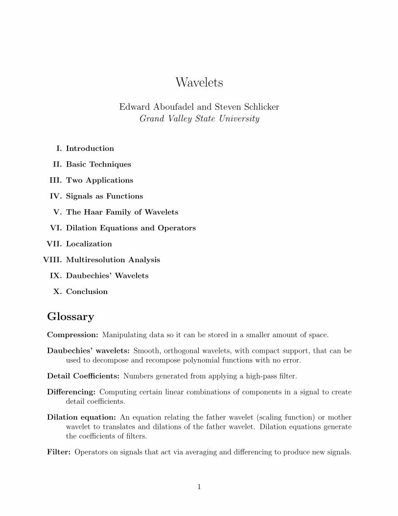
Left: Plot of original data. Center: Result of low and high pass filters. The plot of the original signal is dashed, the result

of the low pass filter is solid, and the result of the high pass filter is dotted. Right: Reconstruction of signal after thresholding.

The plot of the original signal is dashed, the reconstructed signal is solid.

To process a signal with wavelets, we use filters that are determined by the wavelets.There are two components to each filter – a low pass filter and a high pass filter. Thesefilters come from what are called the father and mother wavelets that define a family ofwavelets. Each family of wavelets gives us different filters. We will use the Haar wavelets toillustrate.

The Haar father wavelet, φ, and Haar mother wavelet, ψ are defined by

φ(t) =

{1, if 0 ≤ t < 1

0, otherwiseand ψ(t) =

1, if 0 ≤ t < 1

2

−1, if 12≤ t < 1

0, otherwise.

(1)

The father wavelet is also called the scaling function. Note that the father and motherwavelets are related by:

φ(t) = φ(2t) + φ(2t− 1) and ψ(t) = φ(2t)− φ(2t− 1). (2)

The low pass filter is determined by the father wavelet. This filter uses the coefficientsfrom (2) to perform an averaging of values of a signal. For the Haar wavelets, the two coef-ficients (1 and 1) are divided by 2 and then used to compute linear combinations of pairs ofelements in the signal (later we will see from where the factor of 2 comes). This results incomputing an average of pairs of elements. For example, the average of the first pair of datapoints in our sample is 0.763+0.433

2= 0.598, the average of the second pair of sample points is

0.103−0.1612

= −0.029, and so on. The result is a new signal half the length of the old one. Inparticular, the result of applying the low pass filter to our original signal is

sl = [0.598, −0.029, −0.346, −0.284, −0.061, 0.099, 0.119, 0.050, −0.021, −0.045, −0.027,0, 0.015, 0.013, 0.004, −0.004].

The high pass filter is determined by the mother wavelet. This time, instead of addingthe data in pairs and dividing by 2, we subtract and divide by 2. This is called differencing.For example, using the first two components of s we obtain 0.763

2− 0.433

2= 0.165, the second

pair yields 0.1032− −0.161

2= 0.132, and so on. When the high pass filter is applied to the

original signal we obtain

4

sh = [0.165, 0.132, 0.026, −0.049, −0.056, −0.022, 0.011, 0.021, 0.013, −0.001, −0.007,−0.006, −0.002, 0.002, 0.003, 0.001].

Note that both sl and sh are half the length of the original signal. We can think of theseshorter signals as signals of length 32 by appending zeroes at either the beginning or theend of the signals. In particular, we can identify sl with a signal s′l of length 32 by attaching16 zeroes to the end of the signal. Similarly, we will view sh as a signal s′h of length 32 byadding 16 zeroes to the beginning of the signal. We attach the zeroes in this way so that wecan view the result of applying the low and high pass filters to s as s′ = s′l + s′h. We can thenplot the signal s′ against the signal s and compare. A graph is shown in figure. The resultof the low pass filter is seen on the interval [0,2.5] while the output from the high pass filterappears on [2.5,5]. We see that the low pass filter, or the averaging, makes a copy of theoriginal signal but on half scale. The high pass filter, or the differencing, keeps track of thedetail lost by the low pass filter. The entries in the signal sh obtained from the high passfilter are called detail coefficients.

To see how these coefficients keep track of the details, it is only necessary to see howthey are used to recover the original signal. Note that if we have an average A = a

2+ b

2of

data points a and b and we know the corresponding detail coefficient C = a2− b

2, then we

can recover both a and b via a = A+C and b = A−C. In this way, the process of applyingthe low and high pass filters is completely reversible.

By applying the low pass filter, a copy of the original signal sl at half scale is created. Wenow apply the low and high pass filters to this new copy to obtain another reduced copy ofthe original signal at one quarter scale, plus more detail coefficients. This gives us anothernew copy of the original signal at one quarter scale

sll = [0.285, −0.315, 0.019, 0.085, −0.033, −0.014, 0.014, 0]

plus corresponding detail coefficients

slh = [0.314, −0.031, −0.080, 0.035, 0.012, −0.014, 0.001, 0.004].

Again, we can attach 0’s at appropriate ends of these signals to produce a signal

s′ll + s′lh + s′h

of length 32.We can continue with this process until we obtain one number that contains a copy of

the original signal at the smallest possible scale. Through this process we have constructeda new signal consisting of the average of all the elements of the original signal, plus all ofthe detail coefficients. In our example, this new signal is

snew =[0.005, 0.014, −0.034, −0.016, 0.300, −0.033, −0.010, 0.007, 0.314, −0.031, −0.080,0.035, 0.012, −0.014, 0.001, 0.004, 0.165, 0.132, 0.026, −0.049, −0.056, −0.022, 0.011, 0.021,0.013, −0.001, −0.007, −0.006, −0.002, 0.002, 0.003, 0.001].

5

This new signal has the same length as the original and contains all of the information theoriginal signal does. In fact, as we discussed above, each step in this processing can bereversed to recover the original signal from this new one. Since no information is lost as aresult of applying these filters, this process is called lossless. The entries in snew obtained inthis way are called wavelet coefficients.

III. Two Applications

A. Thresholding and Compression

While the above process shows a new way to store a signal, it is important to see what benefitsthis provides. Recall that the detail coefficients are obtained by averaging the differences ofpairs of data points. Notice that the data points collected from our damped oscillation areclose together in value near the end of the graph. When we process with our high pass filter,the differencing generates values that are close to 0 in our signal, snew. When the detailcoefficients are near 0, there is not much detail in certain parts of the original signal, that isthe signal has fairly constant values there. If we replace all of the detail coefficients that areclose to 0 with 0, then reverse the processing with the low and high pass filters, we shouldobtain a signal that is reasonably close to the original. In other words, when the data issimilar in small groups like this, we will lose little information in the signal if we replace allof these values that are “close together” with the same value.

Returning to our example, let’s assume “close” to 0 means within 0.01. In other words,replace all of the entries in the processed signal that are closer to 0 than 0.01 with a value of0. This is called hard thresholding. After hard thresholding we obtain the processed signal

[0, 0.014, −0.034, −0.016, 0.300, −0.033, 0, 0, 0.314, −0.031, −0.080, 0.035, 0.012, −0.014,0, 0, 0.165, 0.132, 0.026, −0.049, −0.056, −0.022, 0.011, 0.021, 0.013, 0, 0, 0, 0, 0, 0, 0].

To reverse the processing, the first step is to use the final average, 0, along with the finaldetail coefficient, 0.014, to recover the signal on 1

32scale. Note that we introduce some error

in this process by rounding. However, we will tolerate this in the interest of saving space inthe discussion. This gives us [0 + 0.014, 0− 0.014] = [0.014,−0.014]. The result of our firststep in deprocessing the signal is

[0.014, −0.014, −0.034, −0.016, 0.300, −0.033, 0, 0, 0.314, −0.031, −0.080, 0.035, 0.012,−0.014, 0, 0, 0.165, 0.132, 0.026, −0.049, −0.056, −0.022, 0.011, 0.021, 0.013, 0, 0, 0, 0, 0,0, 0].

Continuing in this manner, we reconstruct an imperfect copy of the original signal on fullscale:

[0.759, 0.429, 0.098, −0.166, −0.325, −0.377, −0.338, −0.240, −0.121, −0.009, 0.073, 0.117,0.127, 0.105, 0.067, 0.025, −0.005, −0.031, −0.042, −0.042, −0.044, −0.044, −0.016, −0.016,0.002, 0.002, 0.002, 0.002, 0.002, 0.002, 0.002, 0.002].

6

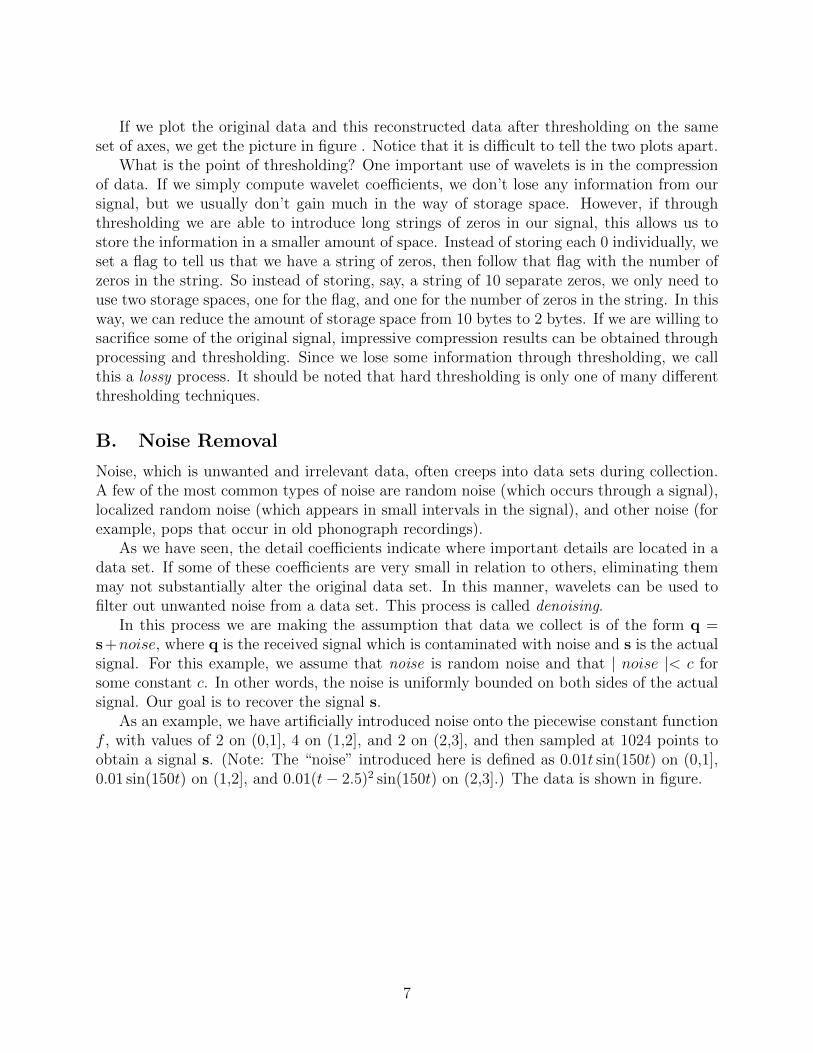
If we plot the original data and this reconstructed data after thresholding on the sameset of axes, we get the picture in figure . Notice that it is difficult to tell the two plots apart.

What is the point of thresholding? One important use of wavelets is in the compressionof data. If we simply compute wavelet coefficients, we don’t lose any information from oursignal, but we usually don’t gain much in the way of storage space. However, if throughthresholding we are able to introduce long strings of zeros in our signal, this allows us tostore the information in a smaller amount of space. Instead of storing each 0 individually, weset a flag to tell us that we have a string of zeros, then follow that flag with the number ofzeros in the string. So instead of storing, say, a string of 10 separate zeros, we only need touse two storage spaces, one for the flag, and one for the number of zeros in the string. In thisway, we can reduce the amount of storage space from 10 bytes to 2 bytes. If we are willing tosacrifice some of the original signal, impressive compression results can be obtained throughprocessing and thresholding. Since we lose some information through thresholding, we callthis a lossy process. It should be noted that hard thresholding is only one of many differentthresholding techniques.

B. Noise Removal

Noise, which is unwanted and irrelevant data, often creeps into data sets during collection.A few of the most common types of noise are random noise (which occurs through a signal),localized random noise (which appears in small intervals in the signal), and other noise (forexample, pops that occur in old phonograph recordings).

As we have seen, the detail coefficients indicate where important details are located in adata set. If some of these coefficients are very small in relation to others, eliminating themmay not substantially alter the original data set. In this manner, wavelets can be used tofilter out unwanted noise from a data set. This process is called denoising.

In this process we are making the assumption that data we collect is of the form q =s+noise, where q is the received signal which is contaminated with noise and s is the actualsignal. For this example, we assume that noise is random noise and that | noise |< c forsome constant c. In other words, the noise is uniformly bounded on both sides of the actualsignal. Our goal is to recover the signal s.

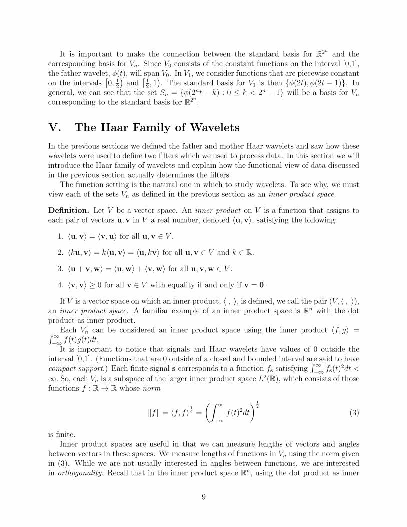
As an example, we have artificially introduced noise onto the piecewise constant functionf , with values of 2 on (0,1], 4 on (1,2], and 2 on (2,3], and then sampled at 1024 points toobtain a signal s. (Note: The “noise” introduced here is defined as 0.01t sin(150t) on (0,1],0.01 sin(150t) on (1,2], and 0.01(t− 2.5)2 sin(150t) on (2,3].) The data is shown in figure.

7

Left: Piecewise constant signal with added noise. Center: Wavelet coefficients of noisy data. Right: Reconstructed piecewise

constant signal after thresholding.

We process this signal to obtain the signal snew, which consists of wavelet coefficients. Aplot of snew is shown in figure. The vertical axis in this figure is scaled so that the noise canbe clearly seen. Other detail coefficients do not completely fit in this window.

Since the actual signal s is mostly constant, we should expect the majority of detailcoefficients to be 0. However, the added noise makes many of these entries small, but non-zero. If we apply thresholding to eliminate what appears to be the added noise, we shouldbe able to recover the signal s. After applying hard thresholding with a tolerance λ = 0.0075and reversing the processing, we obtain the “denoised” data shown in figure.

Similar ideas may be used to restore damaged video, photographs, or recordings, or todetect corrosion in metallic equipment. This approach has also been used in the correctionof seismic data in Japan. However, it should be noted here that the Haar wavelets wereeffective in denoising the signal in this section because of the piecewise constant nature ofthe signal. Later we will see examples of other types of wavelets that are better choices forthe applications mentioned here.

IV. Signals as Functions

When working with wavelets it is convenient to describe our data in terms of functions.There is a simple way to do this which we describe in this section.

In the previous section we began with an initial signal, s, of length 32 or 25. Note thatthis is only one of infinitely many signals of length 32. For convenience, we will denote thecollection of all signals of length 2n by R2n and write s ∈ R32.

There is a natural connection between the space R2n of signals and the space of realvalued functions. We can think of each signal in R2n as representing a piecewise definedfunction on the interval [0, 1] as follows. Break the interval into 2n subintervals of equallength. The function identified with the signal has constant values on each subinterval, withthe value of the function on the ith subinterval given by the ith entry of the signal. Forexample, the signal [1,2,3,4] in R4 corresponds to the function f that has values of 1 on[0, 1

4

), 2 on

[14, 1

2

), 3[

12, 3

4

), 4 on

[34, 1), and 0 elsewhere.

We will denote the collection of all piecewise constant functions on such intervals of length1

2nby Vn. Our signal from the first section is then viewed as a function in V5. Similarly, the

father and mother Haar wavelets (1) can be viewed as functions in V2 and identified withthe vectors [1,1,1,1] and [1,1,−1,−1] in R4.

8

It is important to make the connection between the standard basis for R2n and thecorresponding basis for Vn. Since V0 consists of the constant functions on the interval [0,1],the father wavelet, φ(t), will span V0. In V1, we consider functions that are piecewise constanton the intervals

[0, 1

2

)and

[12, 1). The standard basis for V1 is then {φ(2t), φ(2t − 1)}. In

general, we can see that the set Sn = {φ(2nt − k) : 0 ≤ k < 2n − 1} will be a basis for Vncorresponding to the standard basis for R2n .

V. The Haar Family of Wavelets

In the previous sections we defined the father and mother Haar wavelets and saw how thesewavelets were used to define two filters which we used to process data. In this section we willintroduce the Haar family of wavelets and explain how the functional view of data discussedin the previous section actually determines the filters.

The function setting is the natural one in which to study wavelets. To see why, we mustview each of the sets Vn as defined in the previous section as an inner product space.

Definition. Let V be a vector space. An inner product on V is a function that assigns toeach pair of vectors u,v in V a real number, denoted 〈u,v〉, satisfying the following:

1. 〈u,v〉 = 〈v,u〉 for all u,v ∈ V .

2. 〈ku,v〉 = k〈u,v〉 = 〈u, kv〉 for all u,v ∈ V and k ∈ R.

3. 〈u + v,w〉 = 〈u,w〉+ 〈v,w〉 for all u,v,w ∈ V .

4. 〈v,v〉 ≥ 0 for all v ∈ V with equality if and only if v = 0.

If V is a vector space on which an inner product, 〈 , 〉, is defined, we call the pair (V, 〈 , 〉),an inner product space. A familiar example of an inner product space is Rn with the dotproduct as inner product.

Each Vn can be considered an inner product space using the inner product 〈f, g〉 =∫∞−∞ f(t)g(t)dt.

It is important to notice that signals and Haar wavelets have values of 0 outside theinterval [0,1]. (Functions that are 0 outside of a closed and bounded interval are said to havecompact support.) Each finite signal s corresponds to a function fs satisfying

∫∞−∞ fs(t)

2dt <

∞. So, each Vn is a subspace of the larger inner product space L2(R), which consists of thosefunctions f : R→ R whose norm

‖f‖ = 〈f, f〉12 =

(∫ ∞−∞

f(t)2dt

) 12

(3)

is finite.Inner product spaces are useful in that we can measure lengths of vectors and angles

between vectors in these spaces. We measure lengths of functions in Vn using the norm givenin (3). While we are not usually interested in angles between functions, we are interestedin orthogonality. Recall that in the inner product space Rn, using the dot product as inner

9

product, two vectors u and v are perpendicular if u ·v = 0. Orthogonality is a generalizationof this idea. In an inner product space V , two vectors u and v are orthogonal if 〈u,v〉 = 0.As we will see, orthogonality is a very useful tool when computing projections.

Now we return to wavelets. Recall that we defined the father and mother wavelets by theequations in (1). As the terminology suggests, the father and mother generate “children”.These children are determined by scalings and translations of the parents. In general, thenth generation children are defined by

ψn,k(t) = ψ(2nt− k), 0 ≤ k ≤ 2n − 1. (4)

Note that there are 2n children in the nth generation. The graphs of each of these childrenlook like compressed and translated copies of the mother wavelet.

In the previous section we saw that there is a correspondence between the vector spacesVn and R2n . Consequently, the dimension of Vn is 2n. In fact, we saw earlier that Sn is the“standard” basis for Vn. Another useful basis for Vn is

Bn = {φ, ψ, ψm,k : 0 ≤ k ≤ 2m − 1, 1 ≤ m ≤ n− 1},

which consists of father, mother, and children wavelets. The basis Bn is important in theworld of wavelets precisely because the elements in Bn are the wavelets. The basis Bn alsohas the property that 〈f, g〉 =

∫∞−∞ f(t)g(t)dt = 0 for any f, g ∈ Bn, with f 6= g. In other

words, Bn is an orthogonal basis for Vn.Any time we have an orthogonal basis for a subspace of an inner product space, we can

project any vector in the space onto the subspace. What’s more, there is an elegant way todo this given by the Orthogonal Decomposition Theorem.

The Orthogonal Decomposition Theorem. If {w1,w2, . . . ,wk} is an orthogonal basisfor a finite-dimensional subspace W of an inner product space V , then any v ∈ V can bewritten uniquely as v = w + w⊥, with w ∈ W . Moreover,

w =〈v,w1〉〈w1,w1〉

w1 + · · ·+ 〈v,wk〉〈wk,wk〉

wk =k∑

i=1

〈v,wi〉〈wi,wi〉

wi

and w⊥ = v − w. The vector w in the Orthogonal Decomposition Theorem is called theprojection of v onto W.

This theorem is important in many respects. One way to use this theorem is for approxi-mations. The vector w determined by the theorem is the “best” approximation to the vectorv by a vector in W , in the sense that w⊥ is orthogonal to W . In fact, w⊥ is orthogonal toevery vector in W . The collection of all vectors in V that are orthogonal to every vector inW is a subspace of V . This subspace is called the orthogonal complement of W in V andis denoted W⊥. We then represent the result of the Orthogonal Decomposition Theorem asV = W ⊕W⊥.

To see how this applies to wavelets, let’s return to our earlier example

s = [0.763, 0.433, 0.103, −0.160, −0.320, −0.371, −0.332, −0.235, −0.116, −0.005, 0.077,0.121, 0.129, 0.108, 0.070, 0.029, −0.008, −0.033, −0.045, −0.044, −0.034, −0.020, −0.006,

10

0.006, 0.013, 0.016, 0.015, 0.011, 0.006, 0.001, −0.003, −0.005].

Recall that s is an element of V5. Consider the subspace of V5 spanned by the set C4 ={ψ4,k : 0 ≤ k ≤ 24 − 1}. Now C4 is an orthogonal basis for the space it spans. Let W4

be the span of C4. Using this subspace W4, let us compute the projection of s onto thespace W4 as described in the Orthogonal Decomposition Theorem. Call this vector w. First,note that 〈ψ4,k, ψ4,k〉 = 1

24for any value of k. Let si denote the ith component of s. Now

notice that 〈s, ψ4,k〉 = s2k+2−s2k+1

25for each k. Then the coefficient of ψ4,k in the Orthogonal

Decomposition Theorem is

〈s, ψ4,k〉〈ψ4,k, ψ4,k〉

=s2k+1−s2k+2

25

124

=s2k+1 − s2k+2

2,

which is a detail coefficient as described earlier. The factor of 2 occurs naturally due to thesquares of the norms of our basis vectors. Let a4,k represent the coefficient of ψ4,k in w, sothat a4,k = s2k+2−s2k+1

2. We then have

w =15∑k=0

a4,kψ4,k. (5)

We must treat this projection with caution. Notice that we have only 16 coefficientsin (5). As a result, we can treat w as a signal in R16. In this sense, the coefficients wecalculated when projecting s onto W4 are exactly those we obtained from applying the highpass filter in the first section. In other words, we can say w = sh. When using the OrthogonalDecomposition Theorem, however, we must view this projection as an element of the largerspace, or V5 in this case. To do this, recall that the non-zero components of the vectors inR32 that correspond to ψ4,k ∈ V5 are 1 and −1. When viewed in this way, the vector in R32

corresponding to w (from (5)) will have components

[a4,0,−a4,0, a4,1,−a4,1, . . . , a4,15,−a4,15].

This will be important when we compute w⊥. (This is different from how we earlier extendedsh ∈ R16 to a signal in R32. In that situation, we were interested in interpreting our resultsgraphically. In this case, we are guided by the Orthogonal Decomposition Theorem.)

Now let’s compute w⊥ = s−w. Computing the first two components of w⊥ yields

s1 −w1 = s1 − a4,0ψ4,0(t) = s1 −(

s1 − s2

2

)=

s1 + s2

2,

and

s2 −w2 = s2 + a4,0ψ4,0(t) = s2 +

(s1 − s2

2

)=

s1 + s2

2.

The remaining components can be computed in a similar manner. Looking at the resultcomponentwise, we identify w⊥ with the signal[

s1 + s2

2,s1 + s2

2,s3 + s4

2,s3 + s4

2, . . . ,

s31 + s32

2,s31 + s32

2

].

11

In other words, if we ignore the duplication, we can view w⊥ as the result of applying thelow pass filter to the signal.

Recall that the averaging process (the low pass filter) produces a copy of the originalsignal on half scale. So we can consider the copy, sl, of our signal as a function in V4. It canbe shown that each basis element in B4 is orthogonal to the functions in V4. Consequently,every function in W4 is orthogonal to every function in V4. So V4 and W4 are orthogonalcomplements in V5. In other words, W4 = V ⊥4 and V5 = V4 ⊕ V ⊥4 .

The next step in processing is to decompose the new signal sl in V4. When we apply theOrthogonal Decomposition Theorem to sl, we decompose it into two pieces, one in V3 andone in V ⊥3 as subspaces of V4. This gives us another decomposition of s in V3 ⊕ V ⊥3 ⊕ V ⊥4 .Again, this decomposition uses the idea that we are identifying V3 as subspace of V4, whichis a subspace of V5.

This process continues until we have obtained a vector in

V0 ⊕ V ⊥0 ⊕ V ⊥1 ⊕ V ⊥2 ⊕ V ⊥3 ⊕ V ⊥4 .

In our earlier work, this was the signal snew. Since the coefficients that are determined inthis process are multipliers on wavelets, we can see why they are called wavelet coefficients.We should note here that the process described in the previous sections of constructing newsignals through averaging and differencing has involved successively producing versions ofthe original signal on half scales. Since we continually reduce the scale by half, the processcan only be applied to signals of length 2n some integer n.

VI. Dilation Equations and Operators

In this section we will see how wavelet processing can be viewed as operators that arise fromdilation equations. Again, we use the Haar wavelets to motivate the discussion.

The processing we have done has depended only on the equations (2). These equationsare called dilation equations and they completely determine the process through which thewavelet coefficients are found. In many situations, the properties that we desire our waveletsto have determine the dilation equations for the wavelets.

Once we have dilation equations for a family of wavelets, we can use them to describelow and high pass filters for that family. To make computations more efficient, however, wenormalize the functions in equations (2). Recall that a vector is a normal vector if its normor length is 1. In the case of our wavelets, we use the L2(R) integral norm defined in (3). Asimple integration by substitution shows us that ‖φ(2t)‖ = 1/

√2 = ‖φ(2t− 1)‖.

Multiplying φ(2t) and φ(2t − 1) in the original dilation equations by√

2 to normalizethem produces the dilation equations

φ(t) = h0

√2φ(2t) + h1

√2φ(2t− 1) and ψ(t) = g0

√2φ(2t)− g1

√2φ(2t− 1), (6)

where h0 = h1 = 1√2

and g0 = 1√2

and g1 = − 1√2

for the Haar wavelets.

Suppose we have a signal s = [s0, s1, . . . , s2n−1] of length 2n. The low and high pass filterscan then be described in general by two operators, H (the low pass operator) and G (the

12

high pass operator) defined by

(Hs)k =∑j∈Z

hj−2ksj and (Gs)k =∑j∈Z

gj−2ksj. (7)

The coefficients hi and gi in these sums are called filter coefficients. There are two items tobe aware of here:

• Note the translation in the subscripts of h and g by 2k. If we do a standard convolution(translate by k), the entries we want occur in every other component. We saw thishappen earlier when we used the Orthogonal Decomposition Theorem. Hence, wedownsample at 2k.

• It might seem natural that the High pass operator should be denoted by H, but theconvention is to use G instead.

Notice that for the Haar wavelets these operators give us exactly the results (up to a factorof√

2) that we obtained in the previous section. The importance of this operator approachis that to process signals with wavelets we only need to know the coefficients in the dilationequations. As we will see later, other wavelet families have dilation equations whose coef-ficients are different than those of the Haar wavelets. However, the method of processingsignals with these wavelet families is the same.

To undo the processing with H and G, we define the dual operators denoted H∗ and G∗.The dual operators are defined by

(H∗s∗)k =∑j∈Z

hk−2js∗j and (G∗s∗)k =

∑j∈Z

gk−2js∗j . (8)

Note the change in indices from the definitions of H and G.It is not difficult to see that H∗(Hs) +G∗(Gs) = s for any signal s of length 2n using the

Haar wavelets. However, the orthogonality plays a critical role in this process (recall howorthogonality arose in the projections onto the subspaces Vn and V ⊥n ), so these operatorswon’t perform in the same way if the wavelets we use are not orthogonal. Also, the operatorsdefined by (7) are designed to process signals of infinite length, so there may be difficulties inrecomposing a finite signal at either end if the number of non-zero coefficients in the dilationequations is different than two. This is called a boundary problem and there are severalmethods to cope with such difficulties. We will discuss three such methods in a later section.

VII. Localization

Another important property of wavelets is their ability to identify important information onsmall scale. This is called localization.

In (4) we defined the nth generation children wavelets as contractions and translations ofthe mother wavelet. By selecting a large enough value of n, we are able to analyze our dataon very small intervals. There is, however, no reason to restrict ourselves to small intervals.In fact, the beauty and power of wavelets lies in their ability to perform analysis on both

13

large and small scales simultaneously. To see how this works, we extend the definitions ofthe previously defined sets Vn to include negative values of n as well as to cover functionsdefined (and non-zero) outside of [0,1].

Recall that for non-negative integer values of n, Vn consists of the functions that arepiecewise constant on intervals of length 1

2nwithin the interval [0,1]. If we allow for transla-

tions outside of the interval [0,1], then we can extend the definition of each Vn. We will needto be careful, however, to insist that each of our functions remains in L2(R). With this inmind, V0 will be the space of all functions in L2(R) that are piecewise constant on intervalsof length 1 with integer endpoints. The space V0 will be generated by translations of thefather wavelet of the form φ(t − k) for k ∈ Z. Next, V1 will include all functions in L2(R)that are piecewise constant on intervals of length 1

2with possible breaks at integer points or

at points of the form 2n+12

from some integer n. We can generate functions in V1 with thecollection {φ(2t− k) : k ∈ Z}. Similarly, V2 will be spanned by {φ(22t− k) : k ∈ Z} and willcontain all functions with possible breaks at rational points with denominators of 4 = 22,and so on.

This perspective allows us to define Vn for negative values of n as well. In these cases,instead of contracting the intervals on which our functions are constant, we expand them. Forexample, V−1 will consist of all functions in L2(R) that are piecewise constant on intervalsof length 2, with integer endpoints. More generally, Vn will contain piecewise constantfunctions in L2(R) with possible jumps at points of the form m× 2−n for any integer n. Theset {φ(2nt− k) : k ∈ Z} will generate Vn. An advantage to this approach is that we can nowwork with data that is defined on intervals other than [0,1].

To illustrate this advantage, consider the methods of Fourier analysis, which were dis-cussed in the Introduction. As was previously stated, one disadvantage of Fourier methods isthat they produce global information about signals, but not local information. For instance,if a low-pass filter, based on Fourier analysis, is applied to a signal, then high frequenciesare eliminated throughout the whole signal, which may not be desired. The global approachof Fourier methods can also be seen in the formula for the discrete Fourier transform, whereevery data point contributes to every Fourier coefficient.

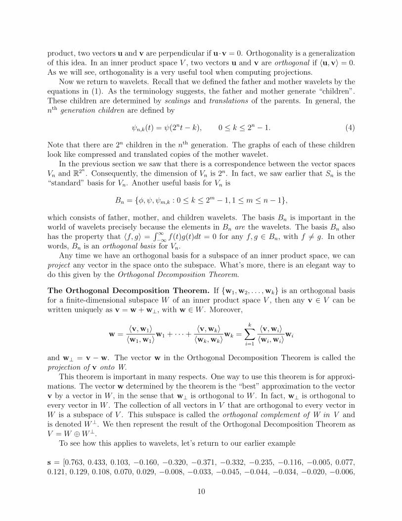
Left: A signal with two short impulses. Right: Selecting wavelets of different scales to analyze a signal.

A wavelet analysis of a signal will bring out local information. As an example, considerthe signal represented on the left in figure. The key behavior of this signal can be foundon the intervals [−4,−2] and [1, 1.5]. If we analyze this signal with wavelets, then specificwavelets will pick up the information on specific intervals. For instance, wavelet coefficients

14

corresponding to the Haar wavelet ψ(2−1t+ 2) ∈ V0, along with scalings of this wavelet thatare in V1, V2, . . ., will be non-zero, due to the impulse on the interval [−4,−2]. Similarly,ψ(2t − 1) ∈ V2 and its scalings in V3, V4, . . ., will notice the impulse on the other interval.All other wavelet coefficients will be zero.

Consequently, translations of ψ can be used to find specific time intervals of interest, andthe scalings of these translations will reveal finer and finer details. This idea is representedon the right in figure. There, the shaded regions correspond to the wavelets we can use toanalyze this function.

VIII. Multiresolution Analysis

In this section we will introduce the idea of a multiresolution analysis within the context ofthe Haar wavelets.

Let’s return to our example processing a signal. There we applied the low and high passfilters to our original signal s, to obtain two new signals, sl and sh, each in R16. Thesesignals correspond to functions in V4. Thses signals sl and sh in R16 (or, consequently, thecorresponding functions in V4) can be thought of in at least two different ways as belongingto R32 (or V5). With such inclusions, we can say that R16 is a subset of R32 (R16 ⊂ R32) or,in the function setting, V4 is a subset of V5 (V4 ⊂ V5). After the first round of processingwith the Haar wavelets, the original signal s in R32 is decomposed into two signals in R32.

The second round of processing consists of applying the low and high pass filters to slwhich yields two new signals sll and slh in R8. Again, each of these signals can be identifiedwith signals in R16 and R32 by an appropriate extension. At each stage of the processing,new signals on half scale are obtained. The processing ends when we are reduced to a singlenumber, a signal in R.

In the function setting, when we process the signal with the low pass filter, a copy ofthe corresponding function from V5 is produced on half scale in V4. Continued processingconstructs additional copies on smaller scales in V3, then V2, and so on until V0 is reached.In other words, we are reproducing our function in a nested sequence of spaces

V0 ⊂ V1 ⊂ V2 ⊂ V3 ⊂ V4 ⊂ V5.

Of course, there is no reason to restrict ourselves to signals of a given length. We can expandthis idea to build a nested collection of sets

· · · ⊂ V−2 ⊂ V−1 ⊂ V0 ⊂ V1 ⊂ V2 ⊂ V3 ⊂ V4 · · ·

that continues for as long as we need in either direction. It can also be shown that theset {φ(t − k)}k∈Z forms an orthogonal basis for V0. These are the basic ideas behind amultiresolution analysis

We have so far only encountered the Haar wavelets, but there are many other families ofwavelets. Wavelets that are typically used in applications are constructed to satisfy certaincriteria. The standard approach is to first build a multiresolution analysis (MRA) and thenconstruct the wavelet family with the desired criteria from the MRA. All of the features ofthe Haar wavelets can be seen in the following definition.

15

Definition. A multiresolution analysis (MRA) is a nested sequence

· · · ⊂ V−1 ⊂ V0 ⊂ V1 ⊂ V2 ⊂ · · ·

of subspaces of L2(R) with a scaling function φ such that

1.⋃

n∈Z Vn is dense in L2(R),

2.⋂

n∈Z Vn = {0},

3. f(t) ∈ Vn if and only if f (2−n) ∈ V0, and

4. {φ(t − k)}k∈Z is an orthonormal basis for V0 (that is, {φ(t − k)}k∈Z is an orthogonalbasis for V0 in which ‖φ(t− k)‖ = 1 for each k ∈ Z).

In every multiresolution analysis there is a dilation equation of the form

φ(t) =∑k

ckφ(2t− k) (9)

The constants ck in a dilation equation are called refinement coefficients. Equations (2) areexamples of dilation equations. As we will see later, dilation equations allow us to constructa wide variety of different types of wavelets.

IX. Daubechies’ Wavelets

A. Dilation Equation for Daubechies’ Wavelets

The idea of a scaling function having compact support is featured in a type of waveletfamily that is named after Ingrid Daubechies, who pioneered their development. The scalingfunctions for Daubechies’ wavelets have compact support and, more importantly, can be usedto accurately decompose and recompose polynomial functions. This property of Daubechies’wavelets is called the regularity property, and it is what makes these wavelets special.

There is more than one family of Daubechies’ wavelets, and one of the simplest familiesis generated by the scaling function called D4. This function has compact support [0, 3], anddue to this compact support, only four of the refinement coefficients are non-zero (hence thesubscript 4). In other words, we can write

D4(t) = c0D4(2t) + c1D4(2t− 1) + c2D4(2t− 2) + c3D4(2t− 3). (10)

The values of the four refinement coefficients are determined by using the fourth propertyof MRAs, an averaging condition for the scaling function, and a regularity condition. Theorthogonality of the translates of D4 yields the following two equations:

c20 + c2

1 + c22 + c2

3 = 2 and c0c2 + c1c3 = 0. (11)

The averaging condition for the scaling function is simply that its average value over the realline is 1. This leads to the equation:

c0 + c1 + c2 + c3 = 2. (12)

16

The regularity condition for D4 will lead to two more equations. The condition states thatconstant and linear functions can be reproduced by D4 and its translates. More specifically,for any real numbers α and β, there exists a sequence of coefficients {ak} such that αt +β =

∑k akD4(t − k). This ability to reproduce polynomials is referred to as regularity or

smoothness, and it distinguishes the different families of Daubechies’ wavelets. For instance,the regularity condition for D6, Daubechies’ scaling function with six refinement coefficients,is that constant, linear, and quadratic functions can be perfectly reproduced.

In some places in the literature, the regularity condition is presented in terms of themother wavelet ψ that corresponds with D4, and the following vanishing moment conditionsare stated instead:

∫∞−∞ ψ(t)dt = 0 and

∫∞−∞ tψ(t)dt = 0. It should be clear that for the family

which is generated byD6, there is a third moment condition to be included:∫∞−∞ t

2ψ(t)dt = 0.Regularity is important for several reasons. First, in image processing, smooth images,

where colors and shades change gradually rather than suddenly, are better analyzed withsmoother wavelets, as edge effects and other errors are avoided. Also, smoother waveletslead to a cleaner separation of signals into low-pass and high-pass pieces. Finally, numericalmethods such as the Fast Wavelet Transform have been found to work more efficiently withwavelets that are more regular.

The regularity condition for D4 leads to these two equations:

−c0 + c1 − c2 + c3 = 0 and − c1 + 2c2 − 3c3 = 0. (13)

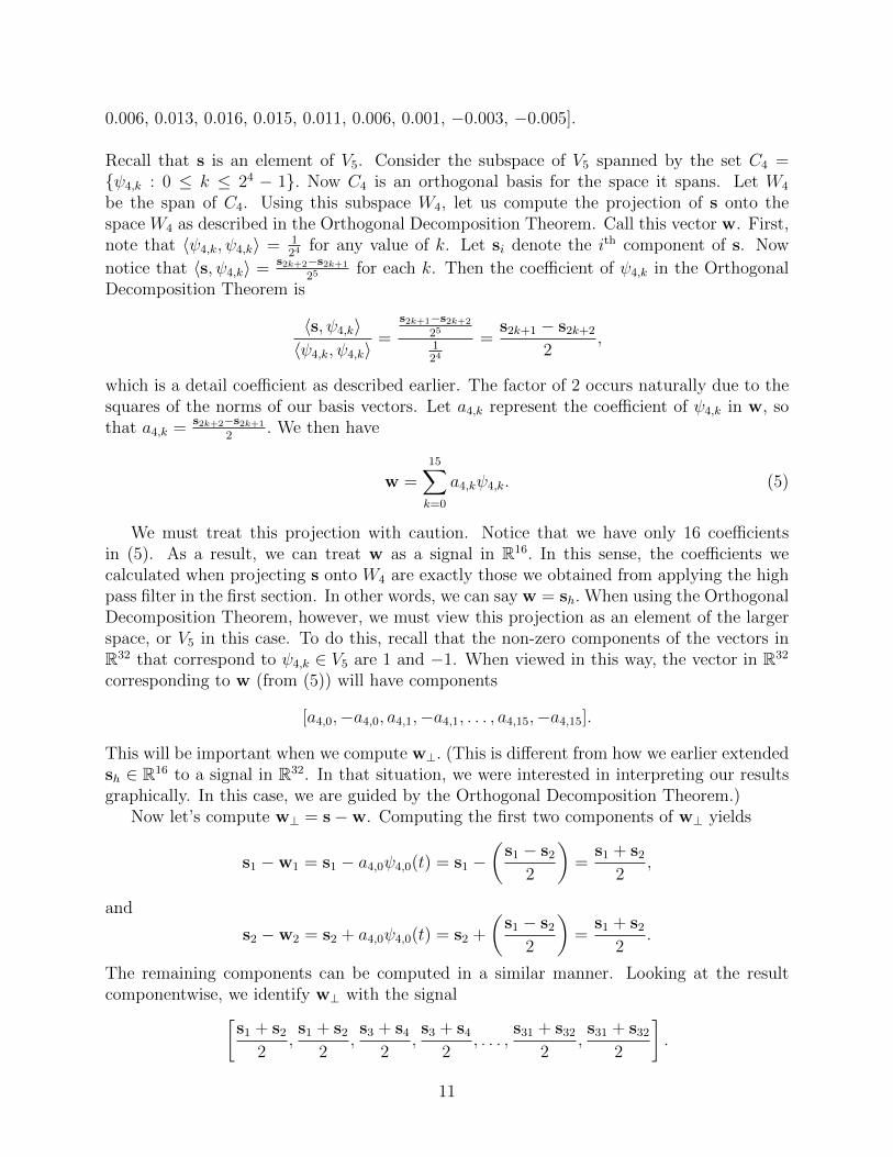
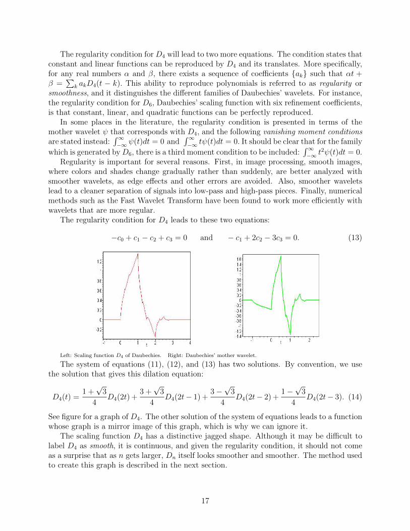
Left: Scaling function D4 of Daubechies. Right: Daubechies’ mother wavelet.

The system of equations (11), (12), and (13) has two solutions. By convention, we usethe solution that gives this dilation equation:

D4(t) =1 +√

3

4D4(2t) +

3 +√

3

4D4(2t− 1) +

3−√

3

4D4(2t− 2) +

1−√

3

4D4(2t− 3). (14)

See figure for a graph of D4. The other solution of the system of equations leads to a functionwhose graph is a mirror image of this graph, which is why we can ignore it.

The scaling function D4 has a distinctive jagged shape. Although it may be difficult tolabel D4 as smooth, it is continuous, and given the regularity condition, it should not comeas a surprise that as n gets larger, Dn itself looks smoother and smoother. The method usedto create this graph is described in the next section.

17

B. The Cascade Algorithm

The Haar wavelets are the simplest, and least regular, type of Daubechies’ wavelets, re-producing constant functions only. Also, the Haar scaling function is the only Daubechies’scaling function that can represented with a simple formula. For other Daubechies’ waveletsfamilies, the scaling functions are generated from the dilation equation using the cascadealgorithm.

The cascade algorithm is based on the dyadic scaling and dilation equation (9) that areat the heart of an MRA. The equation (14) is another dilation equation. These equations canbe used to determine function values at smaller scales, if function values at larger scales areknown. For instance, if φ is known at all multiples of 1

2, then (9) can be used to determine

the value of φ at all multiples of 14.

The cascade algorithm is a fixed-point method. Assuming the refinement coefficients areknown, we can define a mapping from functions to functions by

F (u(t)) =∑k

cku(2t− k). (15)

Fixed points of F will satisfy (9), and it is possible to find these fixed points through aniterative process.

Left: Initial guess for the cascade algorithm. Right: First iteration of the cascade algorithm.

We will demonstrate how this works on (14), and consequently generate D4. To begin,create an “initial guess” for a fixed point of (15), called u0, defined only on the integers. Letu0 be this guess: the function is zero on all of the integers except that u0(0) = 1. Then, toget a good picture, connect these points with line segments, as is done is figure. (This isa reasonable first guess for D4, as we know the scaling function has compact support andreaches some sort of maximum on the interval [0, 3]. Connecting the points is not necessary,except to get good images of the iterates. Also, for normalization reasons, it is importantthat the values of u0 sum to 1.)

Next, use (14) to compute u1 = F (u0) on all multiples of 12, including the integers. For

example,

u1

(3

2

)=

1 +√

3

4u0(3) +

3 +√

3

4u0(2) +

3−√

3

4u0(1) +

1−√

3

4u0(0) =

1−√

3

4.

Once the values on the multiples of 12

are determined, connect the points to create figure.

18

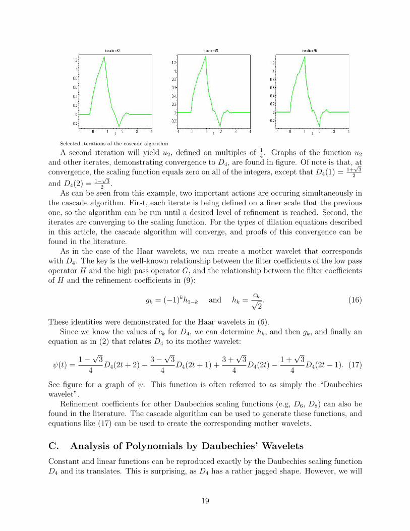
Selected iterations of the cascade algorithm.

A second iteration will yield u2, defined on multiples of 14. Graphs of the function u2

and other iterates, demonstrating convergence to D4, are found in figure. Of note is that, atconvergence, the scaling function equals zero on all of the integers, except that D4(1) = 1+

√3

2

and D4(2) = 1−√

32

.As can be seen from this example, two important actions are occuring simultaneously in

the cascade algorithm. First, each iterate is being defined on a finer scale that the previousone, so the algorithm can be run until a desired level of refinement is reached. Second, theiterates are converging to the scaling function. For the types of dilation equations describedin this article, the cascade algorithm will converge, and proofs of this convergence can befound in the literature.

As in the case of the Haar wavelets, we can create a mother wavelet that correspondswith D4. The key is the well-known relationship between the filter coefficients of the low passoperator H and the high pass operator G, and the relationship between the filter coefficientsof H and the refinement coefficients in (9):

gk = (−1)kh1−k and hk =ck√

2. (16)

These identities were demonstrated for the Haar wavelets in (6).Since we know the values of ck for D4, we can determine hk, and then gk, and finally an

equation as in (2) that relates D4 to its mother wavelet:

ψ(t) =1−√

3

4D4(2t+ 2)− 3−

√3

4D4(2t+ 1) +

3 +√

3

4D4(2t)− 1 +

√3

4D4(2t− 1). (17)

See figure for a graph of ψ. This function is often referred to as simply the “Daubechieswavelet”.

Refinement coefficients for other Daubechies scaling functions (e.g, D6, D8) can also befound in the literature. The cascade algorithm can be used to generate these functions, andequations like (17) can be used to create the corresponding mother wavelets.

C. Analysis of Polynomials by Daubechies’ Wavelets

Constant and linear functions can be reproduced exactly by the Daubechies scaling functionD4 and its translates. This is surprising, as D4 has a rather jagged shape. However, we will

19

demonstrate how a linear function g can be written as a linear combination of D4 and itstranslates. That is, we will show how to determine the values of ak that satisfy

g(t) =∑k

akD4(t− k). (18)

To find the coefficients in the linear combination, the Orthogonal Decomposition Theoremcan be used. For example, according to the theorem, a−2, the coefficient that goes withD4(t+ 2), is defined by

a−2 =〈g(t), D4(t+ 2)〉

〈D4(t+ 2), D4(t+ 2)〉The denominator is 1 because the basis is orthonormal, so the coefficient that goes withD4(t+ 2) is

a−2 =

∫ ∞−∞

g(t)D4(t+ 2)dt.

Since the compact support of D4 is [0, 3], this integral can be written as

a−2 =

∫ 1

−2

g(t)D4(t+ 2)dt. (19)

As discussed earlier, there is no simple formula for D4, as it is simply defined throughits dilation equation, so integrals such as (19) must be computed numerically to as muchaccuracy as desired.

A second approach to determining ak begins by applying a simple change of variables to(18) to get

g(t) =∑j

at−jD4(j).

Using the values of D4 on the integers yields

g(t) = at−1D4(1) + at−2D4(2) = at−11 +√

3

2+ at−2

1−√

3

2. (20)

If we think of ak as a function in k, then it can be proved that ak is a polynomial with thesame degree as g.

We will use this fact to investigate what happens in the cases where g is the constantfunction 1, and where g is the linear function t. If g is constant, then ak is the same constantfor all k, which we will label a. Then (20) becomes

1 = a1 +√

3

2+ a

1−√

3

2= a.

So, ak = 1 for all values of k, and

1 =∑k

D4(t− k). (21)

20

If g is the linear function t, then ak = γk + δ for some constants γ and δ, and (20) is

t = (γ(t− 1) + δ)1 +√

3

2+ (γ(t− 2) + δ)

1−√

3

2,

which simplifies to

t = γt+ (δ − γ(3−√

3

2)).

Therefore, γ = 1, δ = 3−√

32

, and we have the identity

t =∑k

(k +3−√

3

2)D4(t− k). (22)

We now apply this analysis to the specific case of g = 3t + 4. Combining the identities(21) and (22) leads to

3t+ 4 =∑k

(3k +17− 3

√3

2)D4(t− k). (23)

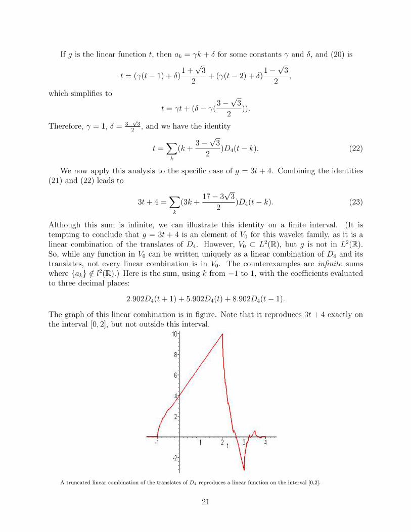
Although this sum is infinite, we can illustrate this identity on a finite interval. (It istempting to conclude that g = 3t + 4 is an element of V0 for this wavelet family, as it is alinear combination of the translates of D4. However, V0 ⊂ L2(R), but g is not in L2(R).So, while any function in V0 can be written uniquely as a linear combination of D4 and itstranslates, not every linear combination is in V0. The counterexamples are infinite sumswhere {ak} /∈ l2(R).) Here is the sum, using k from −1 to 1, with the coefficients evaluatedto three decimal places:

2.902D4(t+ 1) + 5.902D4(t) + 8.902D4(t− 1).

The graph of this linear combination is in figure. Note that it reproduces 3t + 4 exactly onthe interval [0, 2], but not outside this interval.

A truncated linear combination of the translates of D4 reproduces a linear function on the interval [0,2].

21

D. Filters based on Daubechies Wavelets

We now return to a discrete situation, where we wish to process a signal s, rather thananalyze a linear function g, with Daubechies’ wavelets. Two cases will be discussed: aninfinite signal and a finite signal.

The low pass and high pass operators, H and G, defined by (7), will be used to processsignals. For wavelets based on D4, the values of the coefficients in the filter come fromdividing the coefficients in (14) and (17) by

√2, giving us

h0 =1 +√

3

4√

2≈ 0.48296 g−2 =

1−√

3

4√

2≈ −0.12941

h1 =3 +√

3

4√

2≈ 0.83652 g−1 = −3−

√3

4√

2≈ −0.22414

h2 =3−√

3

4√

2≈ 0.22414 g0 =

3 +√

3

4√

2≈ 0.83652

h3 =1−√

3

4√

2≈ −0.12941 g1 = −1 +

√3

4√

2≈ −0.48296.

Since these are the only filter coefficients that are non-zero, the equations in (7) become:

(Hs)k = h0s2k + h1s2k+1 + h2s2k+2 + h3s2k+3 (24)

and(Gs)k = g−2s2k−2 + g−1s2k−1 + g0s2k + g1s2k+1. (25)

For example, consider the infinite signal that is analogous to the example in the previoussection, g = 3t+ 4. For all j, let sj = 3j + 4. Then, (24) and (25) become:

(Hs)k = h0(6k + 4) + h1(6k + 7) + h2(6k + 10) + h3(6k + 13) =√

2(6k +17− 3

√3

2)

and(Gs)k = g−2(6k − 2) + g−1(6k + 1) + g0(6k + 4) + g1(6k + 7) = 0.

There are many observations to make about these results. The output of the low passoperator is, like in the case of the Haar wavelets, an average, but this time it is a weightedaverage, using the four weights h0, h1, h2 and h3. Those specific weights are importantbecause then the high pass operator G will filter the linear signal completely, leaving anoutput of zero. In other words, the details that are critical here are the ones that deviatefrom a linear trend, and, in this case, there are no details. This is why the Daubechies’wavelets are important.

Also of note is that the output of the low-pass operator is similar to the coefficients in(23). Integrals such as (19) also compute weighted averages, but this time in the continuousdomain, so it is reasonable that the results would be quite similar. The different coefficienton k is due to normalization and downsampling.

22

E. Analysis of Finite Signals

In reality, signals that require processing are finite, which presents a problem at the endsof the signal. If a signal s = [s0, s1, . . . , s7] has length 8, then we can compute (Hs)k onlyfor k = 0, 1, and 2. Similarly, we can compute (Gs)k only for k = 1, 2, and 3. If we areever going to have any hope of reconstructing the original signal from average and detailcoefficients, then we will need at least eight of them. There are many ways of addressingthis issue, all of which involve concatenating infinite strings on both ends of s, giving us aninfinite signal that we can process as we did above. Then, we can generate as many averageand detail coefficients as we need.

One approach is called zero padding, and we simply add infinite strings of zeros to bothends of s, giving us:

. . . , 0, 0, 0, s0, s1, s2, s3, s4, s5, s6, s7, 0, 0, 0, . . . .

A second approach is called the periodic method, where we repeat s as if it were periodic,yielding

. . . , s5, s6, s7, s0, s1, s2, s3, s4, s5, s6, s7, s0, s1, s2, . . . .

A third way is called the symmetric extension method, where we create symmetry in thestring by concatenating the the reverse of s and repeating, leading to:

. . . , s2, s1, s0, s0, s1, s2, s3, s4, s5, s6, s7, s7, s6, s5, . . . .

Each method has its advantages. Zero padding is easy to implement. The periodic methodleads to periodic output from the filters. Symmetric extension is popular because it doesnot introduce a sudden change in the signal as the other two do. It is important to observethat each method described here will lead to different results when applying H and G to theextended signals.

For the filters based on D4, there is an overlapping dependence of filter values on datapoints. For this reason, we must use one of these boundary methods. This is not a problemwith the Haar wavelets, however, so signals being processed with the Haar filters do not needto be extended. Finally, the shortest signal that can be processsed by a filter is a concern.The Haar filters can be applied to signals of length 2, but the shortest possible signal for theD4 filters has length 4.

F. A Final Example

At the beginning of this article, we investigated the analysis of a finite signal using the Haarwavelets. In this section, the filters based on D4 will be used to analyze a signal that hasa linear trend, along with some random noise. Through this example, the various ideasdiscussed in this article will come into play.

23

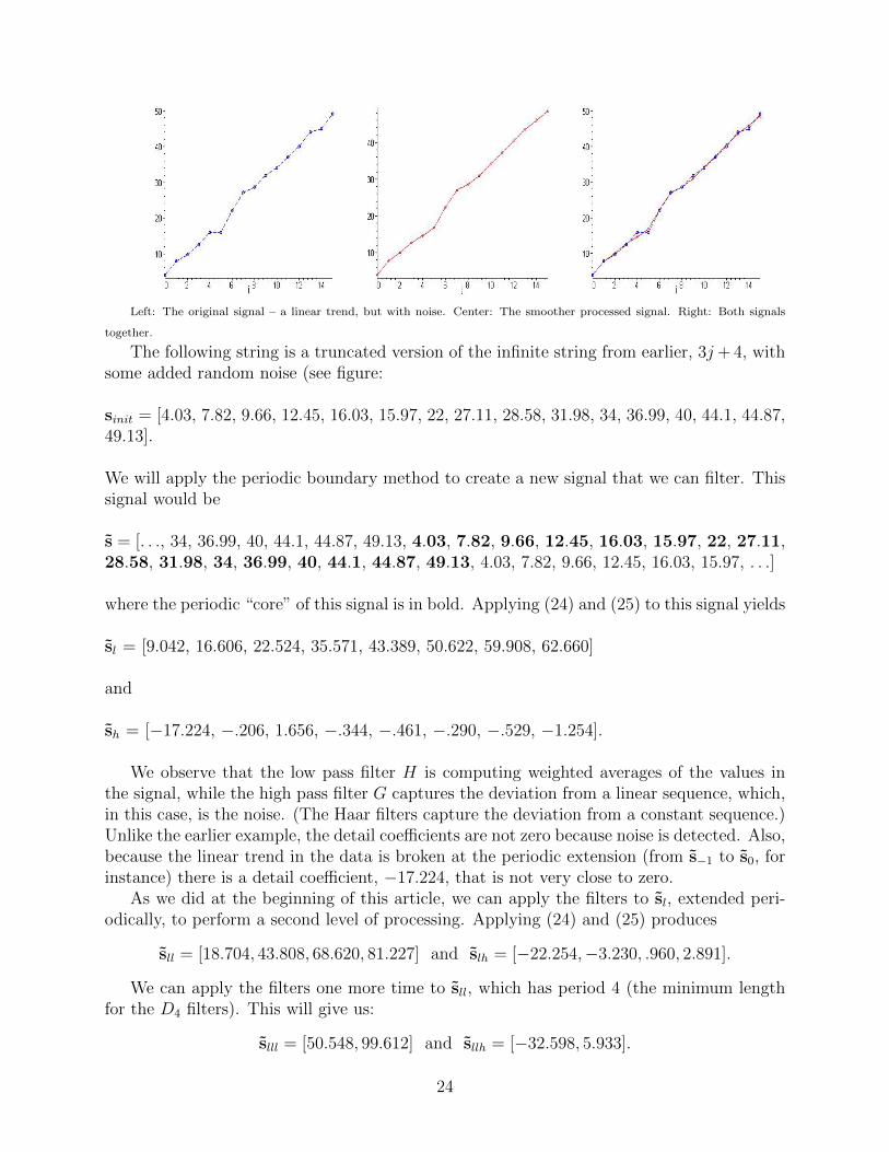
Left: The original signal – a linear trend, but with noise. Center: The smoother processed signal. Right: Both signals

together.

The following string is a truncated version of the infinite string from earlier, 3j+ 4, withsome added random noise (see figure:

sinit = [4.03, 7.82, 9.66, 12.45, 16.03, 15.97, 22, 27.11, 28.58, 31.98, 34, 36.99, 40, 44.1, 44.87,49.13].

We will apply the periodic boundary method to create a new signal that we can filter. Thissignal would be

s = [. . ., 34, 36.99, 40, 44.1, 44.87, 49.13, 4.03, 7.82, 9.66, 12.45, 16.03, 15.97, 22, 27.11,28.58, 31.98, 34, 36.99, 40, 44.1, 44.87, 49.13, 4.03, 7.82, 9.66, 12.45, 16.03, 15.97, . . .]

where the periodic “core” of this signal is in bold. Applying (24) and (25) to this signal yields

sl = [9.042, 16.606, 22.524, 35.571, 43.389, 50.622, 59.908, 62.660]

and

sh = [−17.224, −.206, 1.656, −.344, −.461, −.290, −.529, −1.254].

We observe that the low pass filter H is computing weighted averages of the values inthe signal, while the high pass filter G captures the deviation from a linear sequence, which,in this case, is the noise. (The Haar filters capture the deviation from a constant sequence.)Unlike the earlier example, the detail coefficients are not zero because noise is detected. Also,because the linear trend in the data is broken at the periodic extension (from s−1 to s0, forinstance) there is a detail coefficient, −17.224, that is not very close to zero.

As we did at the beginning of this article, we can apply the filters to sl, extended peri-odically, to perform a second level of processing. Applying (24) and (25) produces

sll = [18.704, 43.808, 68.620, 81.227] and slh = [−22.254,−3.230, .960, 2.891].

We can apply the filters one more time to sll, which has period 4 (the minimum lengthfor the D4 filters). This will give us:

slll = [50.548, 99.612] and sllh = [−32.598, 5.933].

24

Combining slll and sllh with the detail coefficients in above, we create the new signal

snew = [50.548, 99.612,−32.598, 5.933,−22.254,−3.230, .960, 2.891,−17.224,−.206,1.656,−.344,−.461,−.290,−.529,−1.254].

This signal, snew, of length 16 contains all of the information needed to reproduce sinit.The next step in processing this signal is to apply thresholding as a way to remove the

noise. Applying a tolerance of 1.8 to snew to eliminate some of the detail coefficients producess = [50.548, 99.612,−32.598, 5.933,−22.254,−3.230, 0, 2.891,−17.224, 0, 0, 0, 0, 0, 0, 0].

Finally, we apply the dual operators (8) to s and compare our results with sinit. Recon-structing the original signal requires applying the dual operators three times. The first time,we calculate H∗(slll) +G∗(sllh), creating

[18.704, 43.808, 68.620, 81.227].

Continuing this process ultimately yields

[4.003, 7.773, 10.046, 12.721, 14.660, 16.796, 22.359, 27.004, 28.588, 30.993, 34.217, 37.223,40.383, 43.503, 45.919, 48.524].

The original signal and the new signal are compared in figure. Notice that the effect ofprocessing with thresholding is to smooth the original signal and make it more linear. If wehad wished to only denoise the second half of the original signal, then we would have onlyaltered the detail coefficients that are based on that part of the signal.

This example demonstrates many of the ideas discussed in this article. The filters basedon D4 were well-suited for this example, as the original signal had a linear trend, and thefilters effectively separated the linear part of the signal from the noise. Each detail coefficientindicated the extent of the noise in a specific part of the signal. We then reduced the noisethrough thresholding, in effect smoothing the original signal. In this process, we appliedfilters at three different resolutions, until the output of the low pass filter was too short tocontinue.

X. Conclusion

Our discussion in this article has focused on the Haar and Daubechies’ wavelets and theirapplication to one-dimensional signal processing. As we have seen, the main goal in waveletresearch and applications is to find or create a set of basis functions that will capture, in someefficient manner, the essential information contained in a signal or function. Recent workin wavelets by Donoho, Johnson, Coifman and others has shown that wavelet systems haveinherent characteristics that make them almost ideal for a wide range of problems of thistype. This article has just addressed the basic ideas behind wavelets. Additional topics foran interested reader include frames, multiwavelets, wavelet packets, biorthogonal wavelets,and filter banks, to name only a few.

Many results in wavelet theory (the important relationship in (16), for example) aregenerally derived through Fourier analysis. The lack of space and the expository nature

25

of an encyclopedia article motivates the decision to omit such discussion. However, thereis such a close relationship between Fourier analysis and wavelets that it is impossible tothoroughly understand the latter without some knowledge of the former.

Wavelets have become an important tool in many disciplines of science. In areas as di-verse as radiology, electrical engineering, materials science, seismology, statistics, and speechanalysis, scientists have found the key ideas in this subject – multiresolution, localization,and adaptability to specific requirements – to be very important and useful in their work.

26