Wavelet-based Methods for Clutter Removal from Radar

Wind Profiler Data

Lutz A. Justena, Gerd Teschkea and Volker Lehmannb

aZentrum fur Technomathematik, University of Bremen,

Bibliothekstr. 1, 28359 Bremen, GermanybDeutscher Wetterdienst, Am Observatorium 12, 15848 Tauche OT Lindenberg, Germany

ABSTRACT

The common way to process radar wind profiler (RWP) data by moments estimation of the Fourier powerspectrum fails in presence of transient intermittent clutter contributions. Wavelets are especially suitable fordetecting and removing transient components because of their high localization in time and frequency domain.We give an overview on the wavelet filtering of contaminated discrete RWP signals and introduce a new techniqueinvolving the wavelet packet decomposition and a splitting in progressive and regressive signal components. Thistechnique has been successfully tested on severely real-data sets where classical wavelet routines fail.

Keywords: Wavelets, wavelet packets, intermittent clutter filtering, radar wind profiler, signal processing,time-frequency decomposition

1. INTRODUCTION

In recent years, wavelet analysis has become a very powerful tool in applied mathematics. The first applicationsof wavelets were concerned with problems in image/signal analysis/compression. Furthermore, quite recently,wavelet algorithms have also been applied very successfully in numerical analysis, geophysics, meteorology,astrophysics and in many other fields. Especially, it has turned out that the specific features of wavelets canalso be efficiently used for certain problems in the context of radar signal analysis. The aim of this paper is togive an overview on the analysis of discrete RWP data and to explain how wavelets can be utilized for clutterremoval.

The goal of RWP systems is to gather information concerning the three dimensional atmospheric windvector. Radio frequency pulses are emitted and backscattered from small inhomogeneities in the atmosphere.The reflected signal is sampled at certain rates corresponding to different heights. The Doppler shift of theatmospheric (clear-air) signal, which can assumed to be constant over the small measurement period (quasi-stationarity), generates a peak in the Fourier power spectrum. The classical analysis consists of the followingsteps: coherent integration, Fourier analysis, spectral moment estimation, and, finally, the wind estimation.

However, intermittent clutter contributions such as erroneous bird/airplane reflections are well known to benon-stationary (transient), even over short time scales.1–3 As a matter of fact, Fourier transformation cannotresolve transient frequencies. Moment estimation will necessarily fail in these cases. This is exactly the topicwhere wavelet analysis suggests itself since wavelets are by construction very localized functions being ableto resolve frequency transitions during short time periods. Indeed, several wavelet de-noising algorithms havealready been successfully applied.4, 5 It is especially noteworthy that these wavelet algorithms are numericallyvery efficient can be executed on-line on modern PCs.

The clutter removal process consists of three steps.

• First of all, the signal is decomposed into a wavelet series by means of a fast wavelet transform. Sincethe wavelet coefficients contain time as well as frequency information, one speaks of a time-frequency (TF)decomposition.

Further author information:L.A.J.: E-mail: justen@math.uni-bremen.de, Telephone: +49 421 218 4458

• In a second step, a thresholding procedure is applied to identify and remove intermittent clutter from theTF decomposition.

• Finally, the cleared signal is reconstructed from the filtered wavelet coefficients. The Doppler shift can nowbe estimated directly from the cleared Fourier powerspectrum.

The crucial point of the wavelet decomposition is the separation of clutter and clear-air signal. That is, theremust be a certain set of wavelet coefficients containing only clutter information and another set containing onlyclear-air information. If these sets can be identified and do not intersect, removal of the clutter set will lead toa well filtered reconstructed signal which admits a wind estimation by its Fourier spectrum. Hence, the waveletdecomposition should keep each set as small as possible to reduce the risk of intersection.

In Section 2, we will briefly describe how the classical fast dyadic wavelet transform works. Special emphasisis set on TF localization properties and the separability of clear-air signal and clutter. We will see in Sections 3and 4 how the separability can be dramatically improved by splitting the signal into progressive and regressiveparts and afterwards decomposing each part by means of the wavelet packet decomposition. For proofs and morebackground information on wavelets in general and wavelet packets we refer to the book of Mallat.6 Finally, wechoose an adaptive threshold for clutter removal (Section 5) and give some real-data examples (Section 6).

2. DISCRETE WAVELET TRANSFORM

Assume we have a sequence of discrete values a0 = (a0n) sampled from a continuous function f ∈ L2(R) at

intervals of unity length, i.e. a0n = f(n), n ∈ Z. A discrete wavelet transform step decomposes the sequence

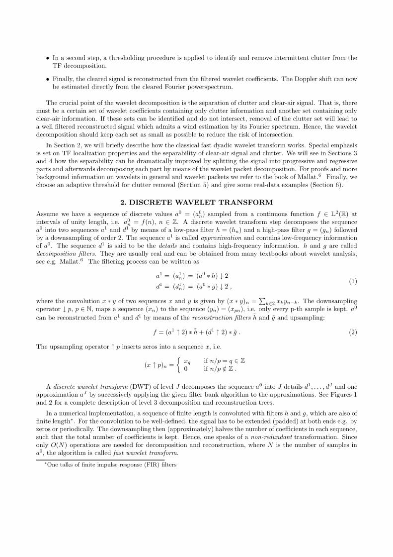
a0 into two sequences a1 and d1 by means of a low-pass filter h = (hn) and a high-pass filter g = (gn) followedby a downsampling of order 2. The sequence a1 is called approximation and contains low-frequency informationof a0. The sequence d1 is said to be the details and contains high-frequency information. h and g are calleddecomposition filters. They are usually real and can be obtained from many textbooks about wavelet analysis,see e.g. Mallat.6 The filtering process can be written as

a1 = (a1n) = (a0 ∗ h) ↓ 2

d1 = (d1n) = (a0 ∗ g) ↓ 2 ,

(1)

where the convolution x ∗ y of two sequences x and y is given by (x ∗ y)n =∑

k∈Zxkyn−k. The downsampling

operator ↓ p, p ∈ N, maps a sequence (xn) to the sequence (yn) = (xpn), i.e. only every p-th sample is kept. a0

can be reconstructed from a1 and d1 by means of the reconstruction filters h and g and upsampling:

f = (a1 ↑ 2) ∗ h + (d1 ↑ 2) ∗ g . (2)

The upsampling operator ↑ p inserts zeros into a sequence x, i.e.

(x ↑ p)n =

{xq if n/p = q ∈ Z

0 if n/p /∈ Z .

A discrete wavelet transform (DWT) of level J decomposes the sequence a0 into J details d1, . . . , dJ and oneapproximation aJ by successively applying the given filter bank algorithm to the approximations. See Figures 1and 2 for a complete description of level 3 decomposition and reconstruction trees.

In a numerical implementation, a sequence of finite length is convoluted with filters h and g, which are also offinite length∗. For the convolution to be well-defined, the signal has to be extended (padded) at both ends e.g. byzeros or periodically. The downsampling then (approximately) halves the number of coefficients in each sequence,such that the total number of coefficients is kept. Hence, one speaks of a non-redundant transformation. Sinceonly O(N) operations are needed for decomposition and reconstruction, where N is the number of samples ina0, the algorithm is called fast wavelet transform.

∗One talks of finite impulse response (FIR) filters

a0 *h

*g

↓2

↓2

a1

d1

*h

*g

↓2

↓2

a2

d2

*h

*g

↓2

↓2

a3

d3

Figure 1. 3 levels of a DWT decomposition filter bank algorithm. The sequence a0 is split into details d1, d2 and d3 andan approximation a3.

a3

d3

↑2

↑2

*h

*g

~

~

+ a2

d2

↑2

↑2

*h

*g

~

~

+ a1

d1

↑2

↑2

*h

*g

~

~

+ a0

Figure 2. 3 levels of a DWT reconstruction filter bank algorithm. The sequence a0 is reconstructed from details d1, d2

and d3 and an approximation a3.

2.1. Time-Frequency Localization Properties

For the wavelet analysis of RWP signals it is of prime importance to know how well certain features can beresolved in time as well as in frequency. In order to get more insight into these time-frequency localizationproperties, it is instructive to look at the sequences of coefficients in Fourier domain. The Fourier transformx = F(x) of a sequence x is defined by

x(ω) = F(x)(ω) =∑

n∈Z

xn exp(−iωn) .

For signals sampled at a time spacing of 1, ω = π is the Nyquist frequency, i.e. the largest frequency which canbe represented without aliasing effects. From the filter bank algorithm described in Figure 1 we know that thesequences of coefficients can be written as

aj = (aj−1 ∗ h) ↓ 2 = (· · · (a0 ∗ h) ↓ 2) ∗ h) ↓ 2) · · · ) ∗ h) ↓ 2) ∗ h) ↓ 2 (3)

dj = (aj−1 ∗ g) ↓ 2 = (· · · (a0 ∗ h) ↓ 2︸ ︷︷ ︸

) ∗ h) ↓ 2︸ ︷︷ ︸

j times

) · · · ) ∗ h) ↓ 2︸ ︷︷ ︸

) ∗ g) ↓ 2︸ ︷︷ ︸

. (4)

The Fourier transforms of a downsampled sequence x ↓ 2 and an upsampled sequence x ↑ 2 are given by

x ↓ 2(ω) =1

2

(x(ω/2) + x(ω/2 + π)

)(5)

x ↑ 2(ω) = x(2ω) . (6)

By taking the Fourier transform on both sides of Equations (3) and (4) and using the convolution theoremx ∗ y = x · y we thus obtain by induction

aj =(a0 ∗ h ∗ (h ↑ 2) ∗ · · · ∗ (h ↑ 2j−2) ∗ (h ↑ 2j−1)

)↓ 2j (7)

dj =(a0 ∗ h ∗ (h ↑ 2) ∗ · · · ∗ (h ↑ 2j−2) ∗ (g ↑ 2j−1)

)↓ 2j . (8)

If we denote the inverse Fourier transform by

x(t) = F−1(x) =1

2π

∫ π

−π

x(ω) exp(iωt) dω ,

we may express Equations (7) and (8) also as

aj =

(

F−1(a0 ·

j−1∏

p=0

h(2p·)))

↓ 2j (9)

dj =

(

F−1(a0 ·

j−2∏

p=0

h(2p·)g(2j−1·)))

↓ 2j . (10)

We posed the question which information of a0 is contained in the wavelet coefficients aj . Equation (9) answersthis question. In Fourier domain, a0 is multiplied by a product of Fourier transformed and scaled low-pass filtersof the form h(2p·). Figure 3 (left) shows plots of |h|2 for several wavelet types. Wavelets are always constructed

such that the energy of h is concentrated in the interval [−π/2, π/2], which justifies the name low-pass filter.

Hence, h(ω) · h(2ω) is concentrated in [−π/4, π/4] and so on. Multiplying a0 with the product filter, onlyenergy at frequencies ω ∈ [−π/2j , π/2j ] is kept. Any energy of a0 at different frequencies is cut off. The finaldownsampling does not change this fact.

The high-pass filter g is complementary to h. Its energy is concentrated in [−π,−π/2]∪[π/2, π]. Repeating theabove analysis for dj shows that dj contains information of a0 at frequencies concentrated in [−π/2j−1,−π/2j ]∪[π/2j , π/2j−1].

Figure 3 (right) illustrates these results in TF domain. The detail coefficients d1 = (a0 ∗ g) ↓ 2 are welllocalized in time since the high-pass filter g consists of only a few non-zero coefficients for most commonly usedwavelets. But frequency localization is rather bad since d1 covers a large amount of the frequency axis. Theopposite is true for a3, where time localization is poor due to the large width of h ∗ (h ↑ 2) ∗ (h ↑ 4), butfrequency localization is better. Also note that all coefficients contain symmetrically negative as well as positivefrequencies. Hence, we cannot distinguish between positive and negative frequencies. In Section 4 we will showhow to overcome this problem.

0

0.5

1

1.5

2

π π/2 0−π −π/2frequency ω

|h|2 , |

g|2

^^

a) b) c)

d1

d2

d3

a3

d3

d2

d1

π

−π

freq

uenc

y ω

π/2

π/4 π/8

0−π/8−π/4

−π/2

time t

Figure 3. Left: 3 decomposition filter pairs |h|2 (solid) and |g|2 (dashed). a) Haar (length 2), b) Daubechies db5 (length10), c) Coifman coif5 (length 30). Right: Schematic overview of the TF coverage of the wavelet coefficients of a level 3DWT.

2.2. Artificial RWP Signal

Let us present an example where we compute the DWT of a pretty much simplified artificial RWP-like signal.The signal shall contain a stationary clear-air signal and a transient airplane echo. The clear-air signal is modeledby a plane wave fair = exp(iωairt), so no Gaussian random distribution is added to its frequency behavior forsimplicity. In order to model the airplane echo, we undertake the following considerations:

• The airplane is more or less a point object, so there should only be one certain Doppler shift at each time,not a distribution of shifts.

• When the airplane approaches the radar site, the Doppler shift is positive.

• When the airplane is right above the site or when its radial velocity component is zero, also the Dopplershift is zero.

• When the airplane leaves the site, the Doppler shift is negative.

A simple model for the behavior of the complex RWP signal is thus a function which linearly decreases itsfrequency. Such a function is called a linear chirp and is given by fclutter = exp(−iωcluttert

2). This modelmatches our observations surprisingly well, as we will see in Section 6. The total RWP signal is the sum of thetwo components, i.e.

f(t) = fair(t) + fclutter(t) = exp(iωairt) + exp(−iωcluttert2)

We choose ωair = 3π4 and ωclutter = π

2·1024 . By this choice, only d1 is influenced by the clear-air signal and theairplane echo frequency exactly matches the Nyquist frequency at the end of the time interval. See Figure 4 fora plot of this signal and a schematic sketch of the TF behavior.

−200 −100 0 100 200

−1

0

1

2

time t

Re

f(t)

−1000 −500 0 500 1000

π

π/2

0

−π

−π/2

time t

freq

uenc

y ω

Airplane echo

clear−air signal

Figure 4. Left: Real part of the artificial RWP signal. Right: Schematic overview of the TF behavior.

After sampling f at t = −1024,−1023, . . . , 1022, 1023 to obtain a complex signal vector (fn) of length 2048,we compute a level 5 DWT using Daubechies db5 wavelet filters containing 10 non-zero coefficients for both hand g. Figure 5 shows a plot of the squared absolute values of the wavelet coefficients.

−1000 −500 0 500 1000

time t

π

π/2

0

−π

−π/2

freq

uenc

y ω

III

III

III

III

II

I

I

Figure 5. Level 5 DWT of f . Box I: clear-air information. Box 2: airplane echo. Box 3: Mixed clear-air signal andairplane echo. Compare also Figure 3.

Coefficients in boxes I contain clear-air information only and must not be removed in a thresholding process.Coefficients in box II contain airplane echo information only and can be filtered without influencing the clear-air signal. Coefficients in boxes III contain mixed information of clutter and signal. A filtering routine wouldinfluence and possibly remove clutter as well as signal information. Note that boxes III cover a large part of theTF plane.

As we said in the introduction, a TF decomposition should keep the set of coefficients containing both clutterand clear-air information (i.e. boxes III) as small as possible. Consequently, we need to look for more suitablemethods to decompose the TF plane.

3. WAVELET PACKETS

We have seen in Section 2 that the DWT may not be suitable for the separation of intermittent clutter andclear-air signal. In cases of high wind speed and slowly-varying airplane echoes there might be many waveletcoefficients containing both clutter and signal information because of the poor frequency localization of thehigh-frequency detail coefficients.

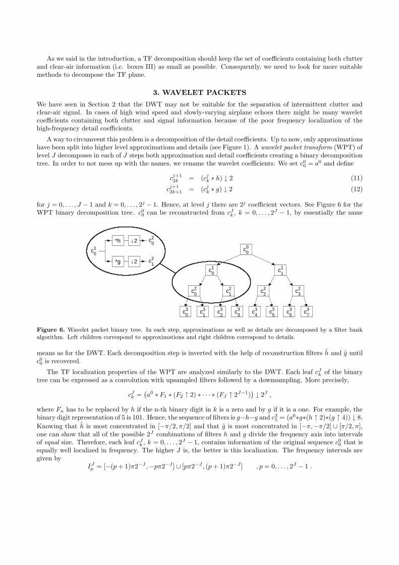
A way to circumvent this problem is a decomposition of the detail coefficients. Up to now, only approximationshave been split into higher level approximations and details (see Figure 1). A wavelet packet transform (WPT) oflevel J decomposes in each of J steps both approximation and detail coefficients creating a binary decompositiontree. In order to not mess up with the names, we rename the wavelet coefficients: We set c0

0 = a0 and define

cj+12k = (cj

k ∗ h) ↓ 2 (11)

cj+12k+1 = (cj

k ∗ g) ↓ 2 (12)

for j = 0, . . . , J − 1 and k = 0, . . . , 2j − 1. Hence, at level j there are 2j coefficient vectors. See Figure 6 for theWPT binary decomposition tree. c0

0 can be reconstructed from cJk , k = 0, . . . , 2J − 1, by essentially the same

c10

c20

c21

*h

*g

↓2

↓2

c00

c10

c11

c20

c21

c22

c23

c30

c31

c32

c33

c34

c35

c36

c37

Figure 6. Wavelet packet binary tree. In each step, approximations as well as details are decomposed by a filter bankalgorithm. Left children correspond to approximations and right children correspond to details.

means as for the DWT. Each decomposition step is inverted with the help of reconstruction filters h and g untilc00 is recovered.

The TF localization properties of the WPT are analyzed similarly to the DWT. Each leaf cJk of the binary

tree can be expressed as a convolution with upsampled filters followed by a downsampling. More precisely,

cJk =

(a0 ∗ F1 ∗ (F2 ↑ 2) ∗ · · · ∗ (FJ ↑ 2J−1)

)↓ 2J ,

where Fn has to be replaced by h if the n-th binary digit in k is a zero and by g if it is a one. For example, thebinary digit representation of 5 is 101. Hence, the sequence of filters is g−h−g and c3

5 = (a0∗g∗(h ↑ 2)∗(g ↑ 4)) ↓ 8.

Knowing that h is most concentrated in [−π/2, π/2] and that g is most concentrated in [−π,−π/2] ∪ [π/2, π],one can show that all of the possible 2J combinations of filters h and g divide the frequency axis into intervalsof equal size. Therefore, each leaf cJ

k , k = 0, . . . , 2J − 1, contains information of the original sequence c00 that is

equally well localized in frequency. The higher J is, the better is this localization. The frequency intervals aregiven by

IJp = [−(p + 1)π2−J ,−pπ2−J ] ∪ [pπ2−J , (p + 1)π2−J ] , p = 0, . . . , 2J − 1 .

cJk contains information of c0

0 at frequencies in IJG[k], where the permutation G can be recursively computed from

G[2k] =

{2G[k] if G[k] is even2G[k] + 1 if G[k] is odd

G[2k + 1] =

{2G[k] + 1 if G[k] is even2G[k] if G[k] is odd

.

Hence, the re-ordered set of vectors (cJG[k])

2j−1

k=0 is frequency-ordered.

Figure 7 (left) illustrates the TF coverage of the leaf vectors. A level 5 WPT of the artificial RWP signalusing Daubechies db5 wavelet filters is shown in Figure 7 (right). Note that, in spite of some artifacts introducedby the WPT, the airplane echo can be expressed by considerably less wavelet coefficients than in the DWT-case.Also boxes III, where clutter and clear-air signal mix, are much smaller.

c22

c23

c21

c20

c20

c21

c23

c22

π

−π

freq

uenc

y ω

3π/4

π/2

π/4

0

−π/4

−π/2

−3π/4

time ttime t

π

π/2

0

−π

−π/2

freq

uenc

y ω

III

III

III

III

II

I

I

−1000 −500 0 500 1000

Figure 7. Left: Schematic overview of the TF coverage of the wavelet coefficients of a level 2 WPT. Note that thehighest frequencies are covered by c2

2 – not c2

3 – due to the permutation G[0, 1, 2, 3] = (0, 1, 3, 2). Right: Level 5 WPTof f . Box I: clear-air information. Box 2: airplane echo. Box 3: Mixed clear-air signal and airplane echo. The two signalcomponents can be much better separated than for the DWT. Compare Figures 5 and 3.

But still, positive and negative frequencies cannot be distinguished. This is due to the fact that we have onlyconsidered real wavelet filters so far. For real wavelets, |h| and |g| are symmetric functions in ω covering partsof the positive frequency axis as well as the negative one. Next section, we shall show how to overcome thisproblem.

4. POSITIVE AND NEGATIVE FREQUENCIES

Consider the complex filters h+n = inhn and h− = (−i)nhn.7 Since h is concentrated in [−π/2, π/2], their

Fourier transforms h+ and h− are concentrated in [0, π] and [−π, 0], resp. We wish to make use of this property.

Before the WPT, we filter c00 with h+ and h−:

+c00 := c0

0 ∗ h+ and −c00 := c0

0 ∗ h− .

+c00 contains information of c0

0 at positive frequencies (progressive part) and −c00 contains information of c0

0 atnegative frequencies (regressive part). +c0

0 and −c00 are then transformed by the WPT separately to obtain

wavelet coefficients +cJk and −cJ

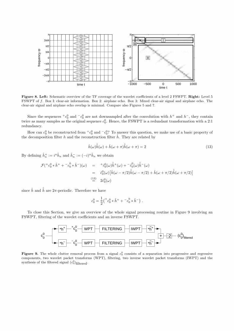
k . The TF domain coverage of these coefficients is similar to last Section, butthis time positive and negative frequencies can be separated, see Figure 8 (left).

Figure 8 (right) shows a plot of this frequency separated wavelet packet transform (FSWPT) of the artificialRWP signal. Airplane echo and clear-air signal overlap only on a very small number of coefficients and can bewell separated.

−c22

−c23

−c21

−c20

+c20

+c21

+c23

+c22

π

−π

freq

uenc

y ω

3π/4

π/2

π/4

0

−π/4

−π/2

−3π/4

time ttime t

π

π/2

0

−π

−π/2

freq

uenc

y ω

III

II

I

−1000 −500 0 500 1000

Figure 8. Left: Schematic overview of the TF coverage of the wavelet coefficients of a level 2 FSWPT. Right: Level 5FSWPT of f . Box I: clear-air information. Box 2: airplane echo. Box 3: Mixed clear-air signal and airplane echo. Theclear-air signal and airplane echo overlap is minimal. Compare also Figures 5 and 7.

Since the sequences +c00 and −c0

0 are not downsampled after the convolution with h+ and h−, they containtwice as many samples as the original sequence c0

0. Hence, the FSWPT is a redundant transformation with a 2:1redundancy.

How can c00 be reconstructed from +c0

0 and −c00? To answer this question, we make use of a basic property of

the decomposition filter h and the reconstruction filter h. They are related by

h(ω)ˆh(ω) + h(ω + π)ˆh(ω + π) = 2 (13)

By defining h+n := inhn and h−

n := (−i)nhn we obtain

F(+c00 ∗ h+ + −c

00 ∗ h−)(ω) = +c0

0(ω)ˆh+(ω) + −c00(ω)ˆh−(ω)

= c00(ω)

[h(ω − π/2)

ˆh(ω − π/2) + h(ω + π/2)

ˆh(ω + π/2)

]

(13)= 2c0

0(ω)

since h and ˆh are 2π-periodic. Therefore we have

c00 =

1

2

(+c00 ∗ h+ + −c

00 ∗ h−

).

To close this Section, we give an overview of the whole signal processing routine in Figure 9 involving anFSWPT, filtering of the wavelet coefficients and an inverse FSWPT.

c00

+c00

−c00

*h+

*h−

WPT

WPT

FILTERING

FILTERING

IWPT

IWPT

*h+

*h−

~

~+ :2 (c0

0)filtered

Figure 9. The whole clutter removal process from a signal c0

0 consists of a separation into progressive and regressivecomponents, two wavelet packet transforms (WPT), filtering, two inverse wavelet packet transforms (IWPT) and thesynthesis of the filtered signal (c0

0)filtered.

5. FILTERING

The main difference between clear-air signal and intermittent clutter like airplane or bird echos is that the formeris stationary, i.e. its average frequency is time-independent, and the latter is transient. Hence, intermittent cluttercan be seen as an inclined line in wavelet coefficient plots such as in Figure 8 (right). It can be well distinguishedfrom the horizontal line representing the clear-air signal.

This difference is exploited in the filtering process. Each vector c ∈ {−cJ0 , . . . ,−cJ

2J−1,+ cJ

0 , . . . ,+ cJ2J−1} carries

information of the signal at a certain well-localized frequency. Note that c corresponds to a single row of thewavelet coefficient plot. Intermittent clutter will show up as a large and narrow peak in (|c2

n|2). Clear-air signals

as well as measurement noise will look like exponentially distributed random samples.8

To remove the peak, we estimate for each c the expectation value 1λ

from (exponentially distributed) samples|cn|

2 which do not belong to the peak, multiply 1λ

by some factor q to achieve a 95% or 99% confidence andremove all samples greater that this threshold s = q

λ, i.e.

(cn)filtered :=

{cn if |cn|

2 ≤ s0 if |cn|

2 > s

for all n. This type of wavelet filtering has been extensively studied by Donoho et al.9, 10 See Figure 10 for anillustration of the thresholding process. We added some Gaussian distributed noise to the artificial RWP signalto make the example more instructive. Intermittent clutter has been completely removed and the clear-air signalhas hardly been touched. The powerspectrum of the reconstructed filtered signal would show a clear peak atDoppler frequency.

time t

π

π/2

0

−π

−π/2freq

uenc

y ω

−1000 −500 0 500 1000

−1000 −500 0 500 10000

5

10

time t

ener

gy

−1000 −500 0 500 10000

5

10

time t

ener

gy

threshold

time t

π

π/2

0

−π

−π/2freq

uenc

y ω

−1000 −500 0 500 1000

cut row−wise remove peak reinsert

Figure 10. Intermittent clutter filtering of the artificial RWP signal plus some noise. Each row of the wavelet transformis filtered separately by thresholding. The threshold is selected adaptively from the coefficients which do not belong to apeak. Note that the clear-air signal is not influenced by this kind of thresholding.

Rows c with stationary components such as clear-air signal and ground clutter are not influenced since thethreshold s will be much higher here. Only removal of peaks carrying both clear-air and intermittent clutterinformation influences the clear-air signal. However, the occurrence of such peaks (boxes III in the plots) is keptto a minimum by construction of the wavelet transform.

6. RESULTS

The special wavelet decomposition and filtering we have developed has proved to remove intermittent clutterfrom an artificial RWP signal very efficiently. Let us now consider a real RWP signal.

The signal as shown in Figure 11 (left) has been recorded by the German weather service with a 482MHz pro-filer in Lindenberg, Germany, at January 19, 1999. It is polluted by a strong airplane echo. The powerspectrumis completely useless for moment estimation in this case (Figure 11 (right)). For simplicity we assume the timespacing between samples to be one such that the frequency axis in the powerspectrum ranges from ω = −π toω = π. This is just a matter of axis scales – the filtering process is completely independent of the time spacing.

Figure 12 shows a plot of the FSWPT wavelet coefficients before (left) and after (right) filtering. We usedSymlet sym10 wavelet filters of length 20 since we found that longer filters reduce artifacts in TF decompositions.

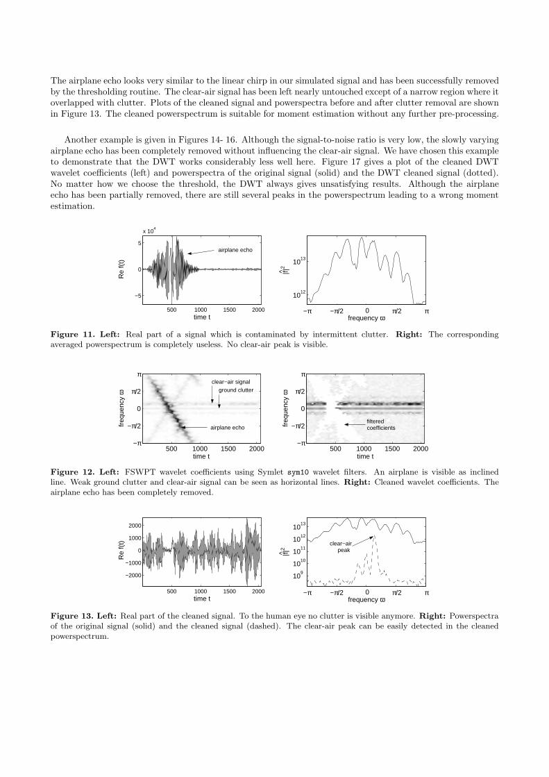
The airplane echo looks very similar to the linear chirp in our simulated signal and has been successfully removedby the thresholding routine. The clear-air signal has been left nearly untouched except of a narrow region where itoverlapped with clutter. Plots of the cleaned signal and powerspectra before and after clutter removal are shownin Figure 13. The cleaned powerspectrum is suitable for moment estimation without any further pre-processing.

Another example is given in Figures 14- 16. Although the signal-to-noise ratio is very low, the slowly varyingairplane echo has been completely removed without influencing the clear-air signal. We have chosen this exampleto demonstrate that the DWT works considerably less well here. Figure 17 gives a plot of the cleaned DWTwavelet coefficients (left) and powerspectra of the original signal (solid) and the DWT cleaned signal (dotted).No matter how we choose the threshold, the DWT always gives unsatisfying results. Although the airplaneecho has been partially removed, there are still several peaks in the powerspectrum leading to a wrong momentestimation.

500 1000 1500 2000

−5

0

5

x 104

time t

Re

f(t)

1012

1013

π π/2 0−π −π/2frequency ω

|f|2

^

airplane echo

Figure 11. Left: Real part of a signal which is contaminated by intermittent clutter. Right: The correspondingaveraged powerspectrum is completely useless. No clear-air peak is visible.

time t

π

π/2

0

−π

−π/2freq

uenc

y ω

500 1000 1500 2000

time t

π

π/2

0

−π

−π/2freq

uenc

y ω

500 1000 1500 2000

airplane echo

clear−air signal ground clutter

filteredcoefficients

Figure 12. Left: FSWPT wavelet coefficients using Symlet sym10 wavelet filters. An airplane is visible as inclinedline. Weak ground clutter and clear-air signal can be seen as horizontal lines. Right: Cleaned wavelet coefficients. Theairplane echo has been completely removed.

500 1000 1500 2000

−2000

−1000

0

1000

2000

time t

Re

f(t)

109

1010

1011

1012

1013

π π/2 0−π −π/2frequency ω

|f|2

^

clear−airpeak

Figure 13. Left: Real part of the cleaned signal. To the human eye no clutter is visible anymore. Right: Powerspectraof the original signal (solid) and the cleaned signal (dashed). The clear-air peak can be easily detected in the cleanedpowerspectrum.

7. CONCLUSIONS

Based on existing wavelet algorithms for clutter removal we have introduced a new type of redundant time-frequency decomposition involving a wavelet packet decomposition combined with a band-pass filter to separateprogressive and regressive signal parts. With this technique we are able to distinguish clutter from clear-aircomponents very precisely. Only very few wavelet coefficients contain information of both components. A hardthresholding routine is applied to remove intermittent clutter. Since the wavelet coefficients are very well localizedin frequency, transient signals appear as narrow peaks and can be easily removed by this method.

Although we have not investigated ground clutter filtering yet, there is definitely a great potential. Groundclutter always appears around zero frequency and can hence be detected and filtered if it does not mix with theclear-air signal. If it does, it is a-priori unclear how to separate them. Reflections from stationary objects likebuildings do not produce a transient signal. We do not see the point in detecting stationary signals with wavelettechniques. This is not what they were build for. Fourier techniques seem more appropriate to us since theyoffer the best frequency localization at the expense of no time localization.

Wavelet algorithms are known for their high numerical efficiency. A DWT only requires O(N) operations,where N is the signal length. Our decomposition needs about 12 times more operations (2N for frequencyseparation, 5N for each of the two level 5 wavelet packet transforms). Modern PCs with CPUs above 1GHzclock frequency can handle these computations in real-time.

We are currently receiving test data from a new Scintec profiler at Frankfurt airport, where a rather highpercentage of data is contaminated by airplane clutter. The algorithms are currently being implemented in C++and will soon be tested on this data.

ACKNOWLEDGMENTS

This project is funded by the European Union in the framework of an EU CRAFT project named MEPROS(www.mepros.de). Gerd Teschke gratefully acknowledges support by DFG grant Te 354/1-2.

REFERENCES

1. J. Wilczak, R. Strauch, F. Ralph, B. Weber, D. Merritt, J. Jordan, D. Wolfe, L. Lewis, D. Wuertz, J. Gaynor,S. McLaughlin, R. Rogers, A. Riddle, and T. Dye, “Contamination of wind profiler data by migrating birds:Characteristics of corrupted data and potential solutions,” J. Atmos. Oceanic Technol. 12, pp. 449–467,March 1995.

2. J. R. Jordan, R. J. Lataitis, and D. A. Carter, “Removing ground and intermittent clutter contamina-tion from wind profiler signals using wavelet transforms,” J. Atmos. Oceanic Technol. 14, pp. 1280–1297,December 1997.

3. J.-C. Boisse, V. Klaus, and J.-P. Aubagnac, “A wavelet transform technique for removing airplane echosfrom ST radar signals,” J. Atmos. Oceanic Technol. 16, pp. 334–346, March 1999.

4. V. Lehmann and G. Teschke, “Wavelet based methods for improved wind profiler signal processing,” Ann.Geophysicae 19, pp. 825–836, 2001.

5. G. Teschke, Waveletkonstruktion ueber Unschaerferelationen und Anwendungen in der Signalanalyse. PhDthesis, University of Bremen, 2001.

6. S. Mallat, A Wavelet Tour of Signal Processing, Academic Press, San Diego, CA, USA, 1999.

7. F. C. A. Fernandes, R. v. Spaendonck, M. J. Coates, and S. Burrus, “Directional Complex-Wavelet Pro-cessing,” Proceedings of Society of Photo-Optical Instrumental Engineers—SPIE2000, Wavelet Applicationsin Signal Processing VIII, San Diego. , 2000.

8. D. S. Zrnic, “Simulation of weatherlike doppler spectra and signals,” J. Appl. Meteor. 14, 1975.

9. D. Donoho and I. Johnstone, “Minimax estimation via wavelet shrinkage,” Tech. Rep. 402, Dept. of Statis-tics, Stanford University, 1992.

10. D. Donoho, I. Johnstone, G. Kerkyacharian, and D. Picard, “Density estimation by wavelet thresholding,”tech. rep., Dept. of Statistics, Stanford University, 1993.

500 1000 1500 2000

−500

0

500

time t

Re

f(t)

108

109

1010

1011

π π/2 0−π −π/2frequency ω

|f|2

^

clear−airpeak

airplane echopeaks

decompositionartifacts

Figure 14. Left: Real part of another signal which is contaminated by slowly varying intermittent clutter. Right: Thecorresponding averaged powerspectrum contains a clutter peak which is more than 20db higher than the clear-air peak.Usual moment estimation techniques would fail here.

time t

π

π/2

0

−π

−π/2freq

uenc

y ω

500 1000 1500 2000

time t

π

π/2

0

−π

−π/2freq

uenc

y ω

500 1000 1500 2000

clear−air signal

airplane echo

decompositionartifacts

Figure 15. Left: FSWPT wavelet coefficients of the second example using Symlet sym10 wavelet filters. An airplane isvisible as inclined line. The clear-air signal appears as faint horizontal line above π/2. Right: Cleaned wavelet coefficients.The airplane echo has been completely removed.

500 1000 1500 2000

−100

0

100

time t

Re

f(t)

108

109

1010

1011

π π/2 0−π −π/2frequency ω

|f|2

^

clear−airpeak

Figure 16. Left: Real part of the cleaned signal. Right: Powerspectra of the original signal (solid) and the cleanedsignal (dashed). The three clutter peaks have been completely removed and the clear-air peak is left untouched.

500 1000 1500 2000

time t

π

π/2

0

−π

−π/2freq

uenc

y ω

108

109

1010

1011

π π/2 0−π −π/2frequency ω

|f|2

^

clear−airpeak

Figure 17. Left: Cleaned DWT wavelet coefficients of the second example using Symlet sym10 wavelet filters. Theclear-air signal is not visible in this plot and the actual structure of the TF behavior is hidden. Right: Powerspectra ofthe original signal (solid) and the DWT cleaned signal (dotted). Clutter power has been reduced. However, several peaksof size comparable to the clear-air peak prevent a moment estimation.