wavelet-based image processing · wavelet-based image processing to berlina james s. walker...

WAVELET-BASED IMAGE PROCESSING

To Berlina

James S. WalkerDepartment of Mathematics

University of Wisconsin–Eau Claire

[email protected]

Abstract The 1990’s witnessed an explosion of wavelet-based methods in the fieldof image processing. This paper will focus primarily on wavelet-basedimage compression. We shall describe the connection between waveletsand vision and how wavelet techniques provide image compression al-gorithms that are clearly superior to the present jpeg standard. Inparticular the wavelet-based algorithms known as spiht, aswdr, andthe new standard jpeg2000, will be described and compared. Our com-parison will show that, in many respects, aswdr is the best algorithm.Applications to denoising will also be briefly referenced and pointerssupplied to other references on wavelet-based image processing.

Keywords: Wavelets, Image Processing, Image Compression

Introduction

The field of image processing is a huge one. It encompasses, at thevery least, the following areas: 1. Image Compression; 2. Image De-noising; 3. Image Enhancement; 4. Image Recognition; 5. Feature De-tection, 6. Texture Classification. Wavelet-based techniques apply toall of these topics. One reason that wavelet analysis provides such anall-encompassing tool for image processing is that a similar type of anal-ysis occurs in the human visual system. To be more precise, the humanvisual system performs hierarchical edge detection at multiple levels ofresolution — and wavelet transforms perform a similar analysis (more onthis below).

Rather than attempting to describe in detail how wavelets apply toall of the areas listed above (that would take an entire book), we focusinstead on the first topic, image compression. For those readers whodesire to study Topic 2, image denoising, see [30], [29], [13], or [18].

1

2

Topics 3 to 5 are explained at an elementary level in [26], where furtherreferences can be found. Topic 6 is discussed in [9].

In this paper we shall provide a broad overview of image compression,especially highlighting a comparison between different image compres-sion algorithms. Mathematical details can be found in [30], [27], and[28], which are all available for downloading at the following webpage:

http://www.uwec.edu/walkerjs/ISAAC2003/WBIP/ (1)

The first part of the paper summarizes transform-based compression,including wavelet-based compression.1 One type of transform-basedcompression is the block-dct

2 method used in the jpeg3 algorithm.

The jpeg algorithm (.jpg files) is widely used for sending images overthe Internet and in digital photography. Wavelet-based algorithms out-perform the jpeg algorithm. The new jpeg algorithm, jpeg2000, usesa wavelet transform instead of a block-dct. Below we shall comparejpeg with jpeg2000 and two other wavelet transform-based algorithms(spiht

4 and aswdr5). This comparison comprises the second part of

our paper. Our comparison will show that, in many respects, aswdr isthe best algorithm. It even outperforms jpeg2000.

1. Transform-based compression and wavelets

Wavelet-based compression is one type of transform-based compres-sion. In general, transform-based compression is done according to thescheme shown in Fig. 1. For wavelet-based compression, a wavelet trans-form and its inverse are used for the transform and inverse transform,respectively. Other transforms can be used as well. For example, thejpeg algorithm uses a block-dct and its inverse (see subsection 1.3 be-low).

The types of images that we shall consider are digital. The image isa matrix of integers ranging from 0 to 255. These values specify shadesof grey— with 0 being pure black and 255 pure white. These integerscan be specified using 8 bits (1 byte) for each pixel (matrix element).

It is typical in image compression to treat grey scale images only. Thatis because the human visual system responds much more sensitively tointensity (corresponding to a grey scale) than to color attributes. See[33, Chap. 9] for more details, including interesting photos in Plate 7.

1Those readers familiar with image compression may skip (or lightly skim) this first part.2Block-Discrete Cosine Transform3Joint Photographic Expert Group4Set Partitioning In Hierarchical Trees5Adaptively Scanned Wavelet Difference Reduction

Wavelet-based Image Processing 3

Image → Transform →Encodetransformvalues

→CompressedImage

Compression Process

CompressedImage

→Decodetransformvalues

→InverseTransform

→ Image

Decompression Process

Figure 1. Transform-based Compression

(a) (b)

(c) (d)

Figure 2. (b) A 200:1 compression of the image in (a). (d) An update of the com-pression, where the roi indicated in (c) is reconstructed exactly in (d). To transmitthe image in (d) requires 30, 435 bytes. A savings of 8.6 to 1 over the full 262, 159bytes for the original. If an exact compression were done for the whole image, thesavings would only be 1.4 to 1.

4

1.1 Karhunen-Loeve Transform

The optimal linear transform to use (when mean square error6 is used)is the Karhunen-Loeve transform. The Karhunen-Loeve transform is thebest (in terms of minimizing mse) linear transform for “decorrelating”(removing redundancy) from images (see [13] and [6]).

Unfortunately, the Karhunen-Loeve transform is very expensive tocompute; it runs very slowly on a computer, far too slowly for mostapplications. Low complexity, and its consequence of rapid compres-sion and decompression is just one of the desired features of a compres-sion/decompression method (codec).

1.2 Desired features of an image codec

There are several desired features of an image codec. Here is a listof some of the main features and where they prove useful: 1. TargetedCompression Ratio [image archiving, Internet transmission]; 2. Progres-sive/Embedded [web pages; database browsing]; 3. Low complexity/Lowmemory [narrow bandwidth applications]; 4. Region of Interest (roi)[reconnaissance; medical diagnosis]; 5. Operations on compressed data[reconnaissance; denoising]. By Targeted Compression Ratio, we meanthe ability to precisely encode to any desired compression ratio. Pro-gressive/Embedded refers to the ability, at any point in the transmissionof the compressed file, to reconstruct an approximate image. Such afeature is useful for webpages and database browsing. The roi featurerefers to the ability of the compressor to allocate more bits to describingregions of interest, a property which is of obvious importance in recon-naissance. See Fig. 2 for an example of the roi property. Table 1 showshow each of the compression algorithms to be compared here fare withregard to these desiderata. We now turn to a discussion of each of theseimage codecs.

1.3 JPEG codec

The jpeg algorithm is discussed in detail in [17]. It has been the iso7

standard since 1990. It is optimized for 16:1 compression of photographicimages. At 16:1 most photographic images, when compressed with jpeg,

6Mean Square Error (mse) is defined as follows

(mse) =1

N

∑

i,j

|f(i, j) − g(i, j)|2 (2)

where g is an approximating image of f and the sum is over all N pixels.7International Standards Organization


Table 1. Properties enjoyed by image codecs.

Property/codec JPEG SPIHT ASWDR JPEG2000

Targeted Compression no yes yes yes

Progressive yes yes yes yes

Low memory yes no no yes

ROI no no yes yes

Compressed operations no no yes yes

will be perceptually lossless. That is, it is difficult if not impossible toperceive any loss of detail between the original and the decompressedimage. For an example, see Figures 3(a) and (b).

The basic scheme of the jpeg algorithm is to divide a matrix of imagepixels into 8 × 8 submatrices, and then apply a dct to each submatrix.The reason for applying a dct is that, for large images, a dct willapproximate the Karhunen-Loeve transform [20]. An 8 × 8 subimage ishardly large, but the dct plus Huffman compression8 produces excellentresults at low compression levels such as 16:1.

One problem with jpeg, however, is at relatively high compressionratios, such as 64:1, there occur “blocking” artifacts. See Fig. 3(c),Fig. 11(b) and Fig. 12(b). These blocking artifacts are due to the factthat at high compression ratios only one pixel for each 8×8 dct subim-age can be transmitted, and that one pixel typically produces only abackground grey level.

Now that we have briefly described jpeg, we turn to the wavelet-basedcodecs, which generally out perform jpeg.

1.4 Wavelet algorithms

We now describe a few wavelet-based compression algorithms. Thereare numerous sources for more details than we have space for here. See,for instance, [12], [30], [27], [28], [24], and [13]. The essential idea behindwavelet transforms is to iterate invertible smoothing and differencing op-erations and, at each iteration, maintain the same number of pixels as theoriginal image. In Fig. 4, we show how these smoothing and differencing

8See [32] for a good introduction to Huffman compression, and [1] for a more thoroughdiscussion.

6

(a) Original (b) 16:1 jpeg

(c) 64:1 jpeg (d) 64:1 jpeg2000

(e) 64:1 spiht (f) 64:1 aswdr

Figure 3. Compressions of the Goldhill image.


Image

��

��

@@

@@R

(S1)

�� @@R

(H1) (D1) (V1)Level 1

(S2)

�� @@R

(H2) (D2) (V2)Level 2

(S3) (H3)(D3)(V3)

Level 3

Figure 4. Example of a wavelet transform. (S1) Smoothed subimage obtainedfrom local averaging of image, 1/4 resolution. (H1) Horizontal component subim-age (obtained from localized vertical differencing and localized horizontal averagingof image) (D1) Diagonal component subimage (obtained from localized vertical dif-ferencing and localized horizontal differencing of image) (V1) Vertical componentsubimage (obtained from localized horizontal differencing and localized vertical aver-aging of image). (S2), (H2), (D2), (V2) Iteration of localized averaging and localizeddifferencing applied to (S1) subimage. (S3), (H3), (D3), (V3) Iteration of localizedaveraging and localized differencing applied to (S2) subimage.

8

operations apply to a test image. At Level 1, the image is smoothed(via local averages) and reduced to a 1/4 size lower resolution versionof the original image, and 3 different local differencing operations areperformed — providing edge detection of 3 kinds: horizontal componentimages (vertical edges suppressed), diagonal component images (hori-zontal and vertical edges suppressed), and vertical component images(horizontal edges suppressed). The total number of pixels at this levelis equal to that of the original image. Moreover, this Level 1 transformcan be inverted: From the 4 subimages at Level 1, the original imagecan be reconstructed.

Level 2 of a wavelet transform repeats the averaging and differencingoperations on the Level 1 smoothed subimage. This iterative processcontinues. We have stopped in Fig. 4 at Level 3. The Level 3 transformconsists of a 1/64 size smoothed subimage, and all of the edge subimagescreated by local differencing at each level. The original image can berecovered from this 3-Level transform.

There are three reasons why wavelet transforms have had such a pro-found effect on image processing. Firstly, the process of creating edgesubimages at multiple resolutions is analogous to a process performed bymammalian vision systems (including human vision systems) See [35],[7], [8], and [14]. Secondly, the process by which a wavelet transformis constructed (local averaging and differencing operations at multipleresolutions) is akin to some important methods for analyzing images.It is akin to the Laplacian pyramid method of Burt and Adelson ([2]and [10]) and the Mumford-Shah theorem concerning edges and smoothbackground in images [15]. Thirdly, there is an analogy between wavelettransforms and fractal theory. See [5] for an excellent discussion. Thefractal-like nature of the wavelet transform is particularly evident inFig. 4.

1.4.1 Zerotrees. One aspect of wavelet transforms which has re-ceived considerable attention( see [22], [21], and [30]) is the phenomenonof zerotrees. In Fig. 4 the grey backgrounds of the difference subimagesrepresent very tiny numerical values, essentially zero in size. If eachdifference subimage is quadrupled in size by doubling each dimension,and placed on top of the corresponding difference subimage at the levelpreceding it (horizontal on top of horizontal, etc.), there is considerableoverlapping of grey areas. If this overlapping carries up to Level 1, thenthese overlapping grey values at each level are called zerotrees (providedthey are set to zero, as they are in the image compression algorithmsdiscussed below).


(a) Lena (b) Lena Histogram

(c) Lena Transform (d) Transform Histogram

Figure 5. Lena image and its wavelet transform.

10

1.5 Essentials of wavelet-based compression

Before we look at some particular wavelet-based image compressionalgorithms, it is helpful to look at a specific image and examine a wavelettransform of it. In Fig. 5(a) we show an image commonly used in imageprocessing, known as Lena. Fig. 5(b) shows a histogram for the intensi-ties of the pixels of Lena. Notice that the histogram is widely dispersedover the range from 0 to 255. A measure of this dispersion is entropy,9

which for this image is 7.45. This shows that there is almost no redun-dancy in the 8-bit image values in Lena. A zip compression of Lena, forexample, yields very little compression (about 15% savings in file size).After transforming, however, and setting all values below a threshold of10 to zero, we obtain Fig. 5(c). Fig. 5(c) has an entropy 1.35, which bythe principles of information theory (see [1] or [32]) can be compressedby a factor of about 8/1.35, a savings of about 83%. When the decom-pressed file, corresponding to Fig. 5(c), is inverted the resulting image isexactly the same as the original. Considerably more compression — withsome loss of exactness, but still perceptually the same as the original — isobtained if a higher threshold is used.

The goal of wavelet-transform encoding is to take advantage of redun-dancy in the transformed image and obtain a good reconstruction upondecompression. The entropy of 1.35 of the histogram of the wavelettransform shows that there is a large amount of redundancy in thewavelet transform — visible both in terms of grey background matchingup at multiple resolutions (zerotrees after thresholding), and in termsof non-zero values (significant values after thresholding) also overlap-ping at multiple resolutions (fractal-like aspect). Each of the algorithmsdiscussed below are similar in that they transmit code for locations ofsignificant values in the wavelet transform and successively encode bi-nary expansions, relative to a base threshold, of the non-zero values (bysending the most significant bits, then the next significant bits, etc.).See [27] at the webpage in (1) for more details.

1.6 SPIHT codec

The SPIHT algorithm was one of the first wavelet-based algorithmsto outperform the jpeg algorithm. It generally provides better lookingdecompressions (no blocking artifacts) and smaller mse than jpeg athigher compression ratios than 16:1.

The basic structure of spiht is the following:

9See [1] or [32] for the definition of entropy.


1. Wavelet transform image. (Use Daub 9/7 wavelets.)

2. Initialize scan order and initial threshold.

3. Significance pass. Encode the significance map using code for tran-sitions from insignificant (zerotrees) to significant values. Use alsoa special arithmetic coding based on grouping transform values in2 × 2 submatrices. See [21].

4. Refinement pass. Generate refinement bits for old significant val-ues. This is called bit-plane encoding. See [27] for more details.

5. Divide threshold by 2, repeat Steps 3 and 4. This step allows forthe binary expansions of values of the transform, relative to theinitial threshold.

More details can be found in [21] and [27], the latter reference is availablefor downloading from the webpage cited in (1). We will compare spiht

with jpeg and other algorithms in Section 2.One drawback of spiht is that it has only a couple of the desiderata

specified in Table 1. It allows for targeted compression ratios and isprogressive/embedded, but does not have the roi property (because if azerotree intersects an roi at one location, then the entire zerotree mustbe encoded). For similar reasons, spiht does not allow operations oncompressed data. Finally, because spiht requires the full image trans-form to be held in ram, it does not have the low memory property.

1.7 ASWDR codec

The aswdr algorithm [28] remedies most of the defects of spiht whileproviding more detailed decompressions. The basic structure of aswdr

is the following:

1. Wavelet transform image.

2. Initialize scan order and threshold.

3. Significance pass. Encode new significant values using differencereduction. (More on this below.)

4. Refinement pass. Generate refinement bits for old significantvalues.

5. Update scan order to search through coefficients that are morelikely to be significant at half-threshold. (More on this below).

6. Divide threshold by 2, repeat Steps 3 and 4.

12

(a) (b)

Figure 6. (a) Children in Level 1 Vertical subimage having significant parents inthe Level 2 Vertical subimage, threshold = 32. Each parent induces a 2×2 submatrixof children located within the same general area as the parent. In general, eachtransform value in a subimage at Level k induces a 2 × 2 submatrix of children atthe next higher resolution Level k − 1. (This is discussed in detail in [30].) (b) Newsignificant values in Level 1 Vertical subimage (V1) when threshold is halved to 16.Notice the similarity between the two images. The similarity of the white regionsillustrates that old significant parents tend to have new significant children. Thesimilarity of the grey regions illustrates the preponderance of zerotrees.

The method of difference reduction is the following. Compute binaryexpansions of the number of steps between new significant values (skip-ping over old ones) as one scans through the transform. Replace themost significant bit by the sign of the transform value. Use these signsas delimiters between expansions. For example, suppose new significantvalues are x[2], x[3], and x[14] at positions 2, 3, and 14 in the scan order,and

x[2] = +17, x[3] = −14, x[14] = +18.

These new values are at indices 2, 3, and 14. The steps between newvalues are 2 = (1 0)2, 1 = (1)2, and 11 = (1 0 1 1)2. Difference reductionencoding is then

0 + − 0 1 1 +

For more details on difference reduction, see [27], which is available fordownloading from (1). An elementary arithmetic coding, using Markov-1 statistics10 only, is also performed on the data generated by differencereduction. It is an open problem to find a more effective arithmeticcoding procedure for aswdr.

The unique feature of aswdr is its creation of a new scan order.Because of space limitations, we shall not discuss this in detail here.

10See [3] for a description of Markov-1 arithmetic coding.


The creation of a new scan order is discussed in detail in [27], [30], and[31], which are all available for downloading from the webpage cited in(1). aswdr creates a new scan order for each Level by first scanningthrough insignificant children of significant parents at previous thresh-olds (see Fig. 6), then scanning through insignificant children (of insignif-icant parents at previous thresholds) which have at least one significantadjoining transform value, and then completing the scan by scanningthrough the remaining insignificant transform values. (See [28], or [30],or [31] for more complete discussions of how new scans are created inaswdr.) By creating new scans in this way, aswdr takes advantage ofboth zerotrees and the tendency of new significant children to have oldsignificant parents, and increases the number of transform values whichcan be encoded with as few steps as possible with difference reduction.

We shall compare aswdr with jpeg and spiht below. Since aswdr

encodes the exact locations of significant values, it has both the roi

and operations on compressed data properties. It is also embedded andprogressive. Unfortunately, because aswdr holds the entire wavelettransform in ram and holds the entire scanning order in ram, it doesnot enjoy the low memory property. It is a goal of future research to finda modification of aswdr which does enjoy the low memory property.

1.8 JPEG2000 codec

The jpeg2000 codec, which is the new ISO standard for photographicimage compression, is described in great detail in [25]. Here we shall onlybriefly summarize its main features. jpeg2000 is a block-based methodlike jpeg, but instead of dividing the image into blocks (subimages),jpeg2000 divides the wavelet transform into blocks. See Fig. 7. Becausethe top-left corner block inverts to a low-resolution version of the originalimage, jpeg2000 avoids the blocking artifacts of jpeg. jpeg2000 has allof the desired properties summarized in Table 1. Because jpeg2000 isdescribed in great detail in [25], we now turn to a comparison of thecompression performance of the codecs we have described above.

2. Comparing different codecs

In this section we will compare the different codecs described above.Our discussion will consist of both objective and subjective comparisonsof four different test images: Lena [see Fig. 5(a)], Goldhill [see Fig. 3(a)],Barbara [see Fig. 11(a)], and Airfield [see Fig. 2(a)]. These are ieee

11

test images used throughout the image processing community for testing

11ieee stands for Institute of Electrical and Electronic Engineers.

14

(a) (b)

Figure 7. (a) Subimages in a 6-level wavelet transform. (b) Division of transformvalues into 64 blocks.

Image →

3-levelDaub 9/7wavelettransform

→Remove(S3)subimage

→InverseTransform

Figure 8. Calculation of edge image for computing ec.

image codecs — they vary widely in their relative smoothness of appear-ance, relative abundance of sharp details, and other image qualities. Oursubjective comparisons will be visual comparisons of various decompres-sions of these test images at moderately high to high compression ratios(32:1, 64:1 and 128:1. See Fig. 3 and Figures 11 to 13.12

Because there is no single standard objective measure for determiningthe best decompression at a given compression ratio, we shall presentresults for three objective measures: psnr (Peak Signal to Noise Ratio),ec (Edge Correlation), and wape (Weighted Average of psnr and ec).psnr is defined as follows [in decibel (dB) units]:

(psnr) = 10 log10

(

2552

mse

)

(3)

where mse is the Mean Square Error defined in Eq. (2). ec and wape

have more complicated definitions which we will discuss later. psnr is

12The reader should keep in mind the author’s bias towards his own algorithm (aswdr).Also, those readers who wish to examine how a computer displays Fig. 3 and Figures 11 to13 may download a file (either images.ps or images.pdf) from the webpage given in (1).


(a) (b)

(c) (d)

Figure 9. Process of creating edge detail image for Lena image, shown in (d). (a)Original image. (b) 3-level Daub 9/7 transform of (a). (c) (S3) subimage removedfrom (b). (d) Inverse transform of (c), producing an edge detail image.

the defacto standard used in the image processing community. It is socommonly used for three reasons: (1) because some objective measureis needed; (2) because it is possible to relate mse to theoretical issuesrelated to rate/distortion curves and least-squares minimization in sta-tistical theory more easily than with any other measures ([11] and [13]),and (3) because psnr is a logarithmic measure which correlates with thelogarithmic response to image intensity of the hvs.

Generally speaking, as a rule of thumb, for psnr values that differ byat least 1 dB, the higher psnr will frequently correspond to noticeablybetter decompressions. Another rule of thumb is that if a psnr is above40 dB, then the original image and its decompression will be perceptuallyindistinguishable.

Because psnr is not completely reliable, we introduce two other mea-sures, ec and wape. ec is the ratio of variances for edge details of thedecompressed image versus the original image. It is more sensitive to

16

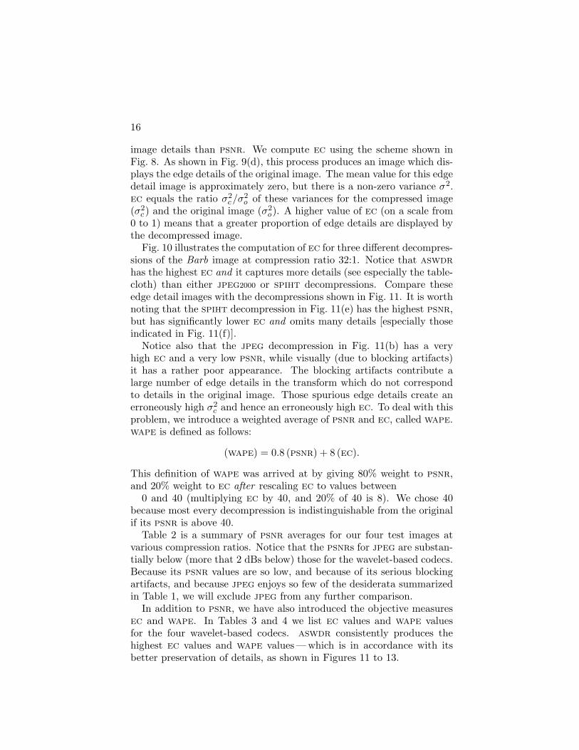
image details than psnr. We compute ec using the scheme shown inFig. 8. As shown in Fig. 9(d), this process produces an image which dis-plays the edge details of the original image. The mean value for this edgedetail image is approximately zero, but there is a non-zero variance σ2.ec equals the ratio σ2

c/σ2o of these variances for the compressed image

(σ2c ) and the original image (σ2

o). A higher value of ec (on a scale from0 to 1) means that a greater proportion of edge details are displayed bythe decompressed image.

Fig. 10 illustrates the computation of ec for three different decompres-sions of the Barb image at compression ratio 32:1. Notice that aswdr

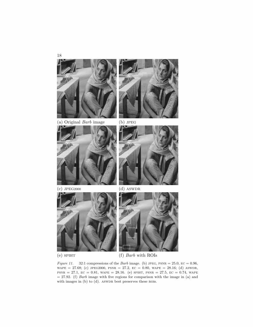
has the highest ec and it captures more details (see especially the table-cloth) than either jpeg2000 or spiht decompressions. Compare theseedge detail images with the decompressions shown in Fig. 11. It is worthnoting that the spiht decompression in Fig. 11(e) has the highest psnr,but has significantly lower ec and omits many details [especially thoseindicated in Fig. 11(f)].

Notice also that the jpeg decompression in Fig. 11(b) has a veryhigh ec and a very low psnr, while visually (due to blocking artifacts)it has a rather poor appearance. The blocking artifacts contribute alarge number of edge details in the transform which do not correspondto details in the original image. Those spurious edge details create anerroneously high σ2

c and hence an erroneously high ec. To deal with thisproblem, we introduce a weighted average of psnr and ec, called wape.wape is defined as follows:

(wape) = 0.8 (psnr) + 8 (ec).

This definition of wape was arrived at by giving 80% weight to psnr,and 20% weight to ec after rescaling ec to values between

0 and 40 (multiplying ec by 40, and 20% of 40 is 8). We chose 40because most every decompression is indistinguishable from the originalif its psnr is above 40.

Table 2 is a summary of psnr averages for our four test images atvarious compression ratios. Notice that the psnrs for jpeg are substan-tially below (more that 2 dBs below) those for the wavelet-based codecs.Because its psnr values are so low, and because of its serious blockingartifacts, and because jpeg enjoys so few of the desiderata summarizedin Table 1, we will exclude jpeg from any further comparison.

In addition to psnr, we have also introduced the objective measuresec and wape. In Tables 3 and 4 we list ec values and wape valuesfor the four wavelet-based codecs. aswdr consistently produces thehighest ec values and wape values — which is in accordance with itsbetter preservation of details, as shown in Figures 11 to 13.


Barb’s edges spiht, ec = 0.74

jpeg2000, ec = 0.80 aswdr, ec = 0.81

Figure 10. ec values for Barb compressions, c.f. Fig. 11.

Table 2. Average psnr values for Airfield, Barbara, Goldhill, and Lena images.

CR\Method JPEG SPIHT JPEG2000 ASWDR

16:1 30.05 32.51 31.91 32.22

32:1 27.93 29.45 28.87 29.21

64:1 25.61 26.92 26.41 26.74

Table 3. Average ec values for Airfield, Barbara, Goldhill, and Lena images.

CR\Method SPIHT JEPG2000 ASWDR

16:1 0.88 0.90 0.92

32:1 0.76 0.80 0.81

64:1 0.61 0.62 0.67

18

(a) Original Barb image (b) jpeg

(c) jpeg2000 (d) aswdr

(e) spiht (f) Barb with ROIs

Figure 11. 32:1 compressions of the Barb image. (b) jpeg, psnr = 25.0, ec = 0.96,wape = 27.68; (c) jpeg2000, psnr = 27.2, ec = 0.80, wape = 28.16; (d) aswdr,psnr = 27.1, ec = 0.81, wape = 28.16. (e) spiht, psnr = 27.5, ec = 0.74, wape

= 27.92. (f) Barb image with five regions for comparison with the image in (a) andwith images in (b) to (d). aswdr best preserves these rois.


(a) Airfield image (b) jpeg


Figure 12. 64:1 compressions of the Airfield image. (b) jpeg, psnr = 21.27, ec

= 0.85, wape = 23.82; (c) jpeg2000, psnr = 23.07, ec = 0.58, wape = 23.04; (d)aswdr, psnr = 23.53, ec = 0.65, wape = 24.02.

Table 4. Average wape values for Airfield, Barbara, Goldhill, and Lena images.

CR\Method SPIHT JEPG2000 ASWDR

16:1 33.05 32.73 33.14

32:1 29.64 29.50 29.84

64:1 26.42 26.09 26.75

20

(a) Original Airfield image (b) spiht


(e) aswdr with rois

Figure 13. 128:1 compressions of the Airfield image. (a) Original image. (b) spiht,psnr = 21.81, ec = 0.44, wape = 20.97. (c) jpeg2000, psnr = 20.90, ec = 0.34,wape = 19.44. (b) aswdr, psnr = 21.70, ec = 0.51, wape = 21.44. (e) Three roisbest preserved by aswdr. (Note: jpeg can only compress airfield to 64:1, it is unableto compress it to 128:1.)


Conclusion

We have discussed several important image codecs, and summarizedtheir compression performance. We close this paper by discussing fouropen problems in image compression.

Open Problem 1. Create a block-based version of aswdr. Of thefour codecs discussed above, aswdr performs the best, but suffers fromhigh memory requirements. jpeg2000 performs almost as well as aswdr

but requires significantly less memory. Since jpeg2000’s low memory re-quirements stem from its block-based structure, we propose the creationof a block-based version of aswdr.

Open Problem 2. How well will aswdr (and/or a low memory ver-sion of aswdr) perform with other transforms? To be precise, how willaswdr perform when the transform is a Generalized Lapped OrthogonalTransform ([16], [19], [23], [4])?

Open Problem 3. Find a better arithmetic coding routine for aswdr.We conjecture that a 3-context method keyed to the 3 different orderingsof transform values in the new scan orderings and/or a grouping of 4neighboring pixels (as with spiht) might yield a better context-basedarithmetic coding than the Markov-1 encoding used at present.

Open Problem 4. Find a better objective measure of compression per-formance than wape, one which accords even better with hvs evaluationof image quality. wape seems to perform well for wavelet-based codecs,but responds too sensitively to the blocking artifacts created by jpeg athigh compression ratios. We conjecture that a weighted average of psnr

and ec values tied to multiple resolution levels (via different weightingsof wavelet transform values in relation to the response of the hvs) mightbe more universally applicable. For initial work in this direction, see[34].

References

[1] Ash, R.B. (1990). Information Theory. New York: Dover.

[2] Burt P.A., and E.H. Adelson. (1983). “The Laplacian pyramid as a compact imagecode.” IEEE Trans. COMM., 31, 532–540.

[3] T.C. Bell, J.G. Cleary, and I.H. Witten. (1990). Text Compression. EnglewoodCliffs, NJ: Prentice-Hall.

[4] Chen, Y.J., S. Oraintara, and K. Amaratunga. “Dyadic-based factorizations forregular paraunitary filter banks and M -band orthogonal wavelets with structuralvanishing moments.” Submitted to IEEE Trans. Signal Processing.

22

[5] Davis G.M. (1998). “A Wavelet-Based Analysis of Fractal Image Compression.”IEEE Trans. on Image Proc., 7, 213-45.

[6] G.M. Davis, and A. Nosratinia. “Wavelet-based Image Coding: An Overview.”Applied and Computational Control, Signals and Circuits, 1, 25-48.

[7] Field, D. J. (1999). “Wavelets, vision and the statistics of natural scenes.” Phil.

Trans. of the Royal Soc., 357, 2527–2542.

[8] Field, D. J., and N. Brady. (1997). “Wavelets, blur and the sources of variabilityin the amplitude spectra of natural scenes.” Vision Research, 37, 3367–83.

[9] Hendricks, B., H. Choi, and R. Baraniuk. (1999) “Analysis of texture segmenta-tion using wavelet-domain hidden Markov trees.” Asilomar Conference on Sig-

nals, Systems, and Computers. Pacific Grove, CA.

[10] Jahne, B. (2002). Digital Image Processing. 5th Ed. Berlin: Springer.

[11] Li J., and S. Lei. (1999). “An embedded still image coder with rate distortionoptimization.” IEEE Trans. on Image Processing, 8, 913-24.

[12] Mallat, S. (1989). “A theory for multiresolution signal decomposition: the waveletrepresentation.” IEEE Trans. Patt. Anal. and Mach. Intell., 11, 674–693.

[13] Mallat, S. (1999). A Wavelet Tour of Signal Processing, 2nd Ed. New York:Academic Press.

[14] Marr D. (1982). Vision. San Francisco, CA: W.H. Freeman.

[15] D. Mumford, and J. Shah. (1989). “Boundary detection by minimizing function-als I.” Image Understanding. New York: Ablex Press.

[16] Nguyen, T.Q., and R.D. Koilpillai. (1996). “Theory and design of arbitrary-length cosine-modulated filter banks and wavelets satisfying perfect reconstruc-tion.” IEEE Trans. on Signal Processing. 44, 473-83.

[17] Pennebaker W.B., and J.L. Mitchell. (1992). JPEG Still Image Compression.

London: Chapman and Hall.

[18] Portilla, J., and E. Simoncelli. (2003). “Image restoration using gaussian scalemixtures in the wavelet domain.” Proceedings 10th International Conference on

Image Processing, Sept. 2003.

[19] Queiroz, R.L., and T.D. Tran. (2001). “Lapped transforms for image compres-sion.” Chap. 5 in The Transform and Data Compression Handbook, (Eds.) Rao,K.R., and P.C. Yip. Boca Raton, FL: CRC/Chapman Hall.

[20] Rao, K.R., and P. Yip. (1990). Discrete Cosine Transform: Algorithms, Advan-

tages, Applications. Boston, MA: Academic Press.

[21] Pearlman, W.A., and A. Said. (1996). “A new, fast, efficient image codec basedon set partitioning in hierarchical trees.” IEEE Trans. on Circuits and Systems

for Video Tech., 6, 243–50.

[22] Shapiro, J.M. (1993). “Embedded image coding using zerotrees of wavelet coef-ficients.” IEEE Trans. Signal Proc., 41, 3445–62.

[23] Oraintara, S. (2000). “Regular linear phase perfect reconstruction filter banksfor image compression.” Ph.D. dissertation, Boston University.

[24] Strang, G., and T.Q. Nguyen. (1996). Wavelets and Filter Banks. Boston, MA:Wellesley-Cambridge Press.

[25] Taubman, D.S., and M.W. Marcellin. (2002). JPEG2000: Image Compression

Fundamentals, Standards and Practice. Boston, MA: Kluwer.


[26] Walker, J.S. (1999). A Primer on Wavelets and their Scientific Applications.

Boca Raton, FL: CRC/Chapman Hall.

[27] Walker, J.S., T.Q. Nguyen. (2001). “Wavelet-based image compression.” Chap. 6in The Transform and Data Compression Handbook, (Eds.) Rao, K.R., andP.C. Yip. Boca Raton, FL: CRC/Chapman Hall.

[28] Walker, J. S., and T.Q. Nguyen. (2000). “Adaptive scanning methods for waveletdifference reduction in lossy image compression.” IEEE Int’l conf. on Image Proc.,

Vancouver, Sept. 2000, 3, 182–85.

[29] Walker, J.S. (2003). “New methods in wavelet-based image denoising.” Progress

in Analysis: Proceedings of the 3rd International ISAAC Congress. (Eds.)H.G.W. Begehr, R.P. Gilbert, and M.W. Wong. New Jersey: World Scientific.

[30] Walker, J.S. (2002) “Tree-Adapted Wavelet Shrinkage.“ Advances in Imaging

and Electron Physics, pp. 343-394, New York: Elsevier Science (USA), 343–94.

[31] Walker, J.S. (2002). “Combined image compressor and denoiser based on tree-adapted wavelet shrinkage.” Optical Engineering, 41, 1520–27.

[32] Walnut, D.F. (2002). An Introduction to Wavelet Analysis. Boston, MA:Birkhauser.

[33] Wandell, B. A. (1995). Foundations of Vision. Sinauer Associates, Sunderland,MA.

[34] Wang, Z., A.C. Bovik, H.R. Sheikh, and E.P. Simoncelli. (2004). “Image qualityassessment: From error measurement to structural similarity.” IEEE Trans. on

Image Processing, 13, To appear.

[35] Watson, A. B. (1987). “Efficiency of a model human image code.” J. Optical Soc.

Am., 4, 2401–17.

wavelet-based image processing · wavelet-based image processing to berlina james s. walker...

Documents