wave wire wash monitoring with … plan ... pcap pcap02a evaluation board ... wire acts as a...
TRANSCRIPT

WAVE WIRE WASH MONITORING WITH INVESTIGATION OF THE EFFECTS OF
SALINITY AND TEMPERATURE ON CAPACITENCE MEASUREMENT
A Thesis submitted for the degree of Masters of Science in
Engineering with Innovation and Entrepreneurship
by
Stephen Peter Rowe, BSc in Mechanical Engineering
Department of Mechanical Engineering
University College London
I, Stephen Peter Rowe, confirm that the work presented in this thesis is my own.
Where information has been derived from other sources, I confirm that this has been
indicated in the thesis.
September 2017
Student Number: 16121681
Total number of words: 11,980

2
Abstract
The purpose of this project is to design a wave height data collector to monitor the water
surface disruption on the River Thames due to increased river traffic during construction of
the Thames Tideway project. The high traffic on the water causes wave wash and disruption
which affects the residential boating communities and the river ecology. The wave monitoring
method is a proven technology that determines wave height via capacitance measurement
between two wires that protrude vertically into the water. The capacitance measurements
vary linearly with the wave height, requiring a simple conversion to obtain wave amplitude
readings. The objective of this project is to design and construct a fully functioning device for
the River Thames while investigating the effects that salinity and temperature of the water
have on the capacitance measurements. Investigations within the project include field
measurements of the fluctuating salinity and temperature of the Thames Estuary, static water
depth tests with varying salinity and temperature, dynamic wave tests in the laboratory wave
generation tank as well as functional tests on the river itself. Results of the static tests show
that change in temperature has significant effect on the wave capacitance measurement with
deviations of approximately 5.56% per 5ºC shift. Salinity changes resulted in negligible effect.
The additional dynamic testing of the device resulted in accurate wave readings averaging
below 10% error for waves at frequencies lower than 1 Hz. This technical report will include a
literature review, discussion of the design criteria, market research, prototyping, testing and
results as well as final conclusions and future steps for the device.

3
Contents Abstract ..................................................................................................................................... 2
Nomenclature ............................................................................................................................ 5
List of Tables .............................................................................................................................. 6
List of Figures ............................................................................................................................. 6
1. Introduction........................................................................................................................ 7
1.1. Background ................................................................................................................. 7
1.2. Aims ............................................................................................................................ 8
1.3. Objectives ................................................................................................................... 8
1.4. Report Structure ......................................................................................................... 9
1.5. Literature Review ........................................................................................................ 9
1.5.1. Wave Wire Technology ........................................................................................ 9
1.5.2. Wash Generation Overview .............................................................................. 12
1.5.3. Environmental Impact ....................................................................................... 13
2. Design Criteria .................................................................................................................. 16
3. Design and Prototyping .................................................................................................... 18
3.1. Hardware Design ....................................................................................................... 19
3.1.1. The Frame .......................................................................................................... 19
3.1.2. The Wires ........................................................................................................... 20
3.1.3. Electronics Encasement ..................................................................................... 21
3.2. Electronics Design ..................................................................................................... 21
3.2.1. Capacitance Measurement................................................................................ 22
3.2.2. Configuration Setpoints ..................................................................................... 23
3.2.3. Microcontroller and Data Computation ............................................................ 23
4. Experiment and Testing Setup ......................................................................................... 25
4.1. Field Measurements ................................................................................................. 25
4.2. Laboratory Tests ....................................................................................................... 25
4.3. Field Tests ................................................................................................................. 27
5. Results .............................................................................................................................. 28
5.1. Laboratory Experiment Results................................................................................. 28
5.1.1. Small-Scale Prototype Testing ........................................................................... 28
5.1.2. Large-Scale Prototype Testing ........................................................................... 30
5.2. Field Test Results ...................................................................................................... 33
6. Discussion ......................................................................................................................... 36
4
6.1. Prototype Performance ............................................................................................ 38
6.2. Future Steps .............................................................................................................. 40
7. Business Plan .................................................................................................................... 43
7.1. Market Size ............................................................................................................... 43
7.2. Entrepreneurial Approach ........................................................................................ 43
7.3. Cost Breakdown ........................................................................................................ 44
7.4. Financing ................................................................................................................... 45
8. Conclusion ........................................................................................................................ 46
References ............................................................................................................................... 48
Appendix .................................................................................................................................. 51

5
Nomenclature
Greek Letters
ε0 permittivity of a vacuum
εr relative dielectric constant
ρ density
τ time constant
ζ wave amplitude, peak to trough
Roman Letters
AWG American wire gauge
C capacitance
CAD computer-aided design
CDC capacitance-to-digital-converter
dq/dt derivative of charge with respect to time
dv/dt derivative of voltage with respect to time
e Euler’s number
Ek potential energy per unit area
Ep potential energy per unit area
Etotal total energy per unit area
EMFF European Maritime and Fisheries Fund
g acceleration of gravity
ic electric current
I2C two wire communication interface
l length of submerged wire
PC personal computer
PCap PCap02a evaluation board
pF pico-farad – capacitive unit of measure
ppt parts per thousand – salinity unit
PTFE polytetrafluoroethylene
PVC polyvinyl chloride
q electric charge

6
R resistance
R1 inner radius of capacitive wire – radius of conductive metal wire
R2 outer radius of capacitive wire – radius of wire insulating material
RC (circuit) Resistor-Capacitor circuit
RLC (meter) Resistance-Inductance-Capacitance meter
SCL serial clock
SDA serial data
t time
Theo theoretical value or measurement v voltage
v0 initial voltage
v(t) voltage function with respect to time
List of Tables
Table 1. List of design criteria. ................................................................................................. 16
Table 2. Prototype components and materials list. ................................................................ 19
Table 3. Percent error statistics for wave generation tests with varying frequency. ............. 32
Table 4. Prototype cost breakdown and future design projections. ....................................... 44
List of Figures
Figure 1. Wave wire capacitor concept diagram. ....................................................................... 8
Figure 2. Voltage response on an RC circuit ............................................................................. 12
Figure 3. Wave wire prototypes. .............................................................................................. 18
Figure 4. Visualisation of capacitive wire tension system. ....................................................... 21
Figure 5. Wave wire electronic system schematic. .................................................................. 22
Figure 6. Initial small-scale prototype testing results. ............................................................. 28
Figure 7. Salinity variation test. ................................................................................................ 29
Figure 8. Temperature variation test results ............................................................................ 30
Figure 9. Large scale prototype static test calibration. ............................................................ 30
Figure 10. Dynamic functional test results, full-scale prototype. 1Hz wave Generation. ....... 31
Figure 11. River test 1 results section. ..................................................................................... 34
Figure 12. River test 2 results section. ..................................................................................... 35
Figure 13. Dynamic functional test results, full-scale prototype. 1.6 Hz wave generation. .... 37
Figure 14. Display of capacitance measurement with rapid change in depth ......................... 37
Figure 15. Updated wave wire frame design including flotsam shield .................................... 42

7
1. Introduction
1.1. Background
The purpose of this project is to design a wave height data collector to monitor the water
disruption on the River Thames due to the increased traffic during the construction of the
Thames Tideway project. The Thames Tideway project is an initiative to improve the quality
of the water of the River Thames by increasing the capacity of the London sewage system. It
is a seven-year project with five years of construction of the underground sewer line. For
construction in Central London, a tunnel excavation machine is lowered at the Kirtling Street
site near Nine Elms where the excavated material is removed and loaded onto 1500-ton
barges that transport the material out of the city via the River Thames.
The construction and high traffic of these large barges is the main issue revolving around this
project. The high traffic on the water causes more wave wash and disruption, which effects
the residential boating communities and the river ecology. This wave monitoring project was
created through the UCL Engineering Exchange and is intended to develop a device that will
measure wave profiles on the River Thames and thus monitor the water traffic. There are
existing technologies that can measure wave heights; however, such devices are normally
used at sea, are high in cost or are not readily available on the market today.
The wave measurement device developed in this project is called a wave wire, which is a
device with vertical wires that are partly submerged through the surface of the water. The
wire acts as a capacitor which is attached to an electrical circuit to charge and discharge. The
wires are normally insulated with a polymer coating that acts as the dielectric of the capacitor.
As shown in Figure 1 below, the two “plates” of the capacitor are the actual conductive wire
(inside the insulating coating) and the surrounding water which is grounded with an uncoated
grounding wire. The capacitance of the wire changes due to the change in the plate size as the
water moves up and down the wire with the passing wave. The circuit is connected to a data
logger which collects the capacitance readings and converts the readings to wave heights due
to the linear relation between the two parameters, which will be discussed in the literature
review.
8
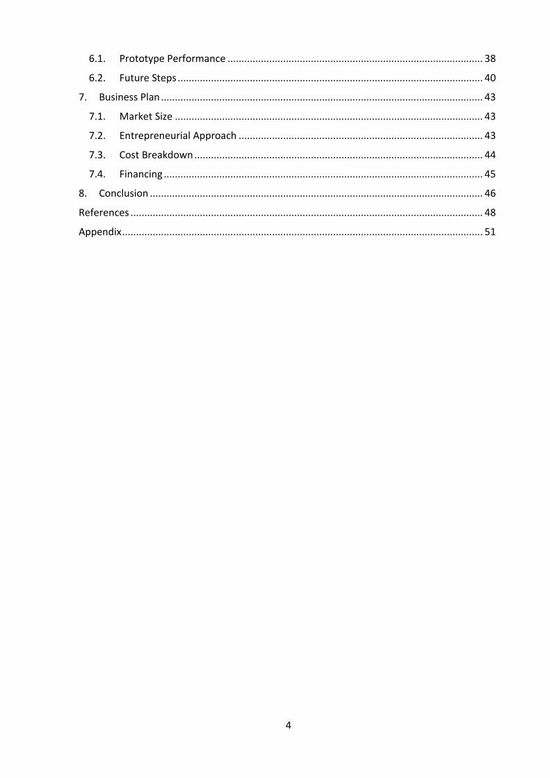
Figure 1. Wave wire capacitor concept diagram. The surface area of the inner conductive core of the capacitive wire (right) is the area of one capacitor plate and the surface area of the insulation material that is submerged in the water is the area of the second plate. The
water is grounded via the uncoated grounding wire. As the second plate changes in area with the passing wave, the capacitance changes.
1.2. Aims
The nature of the River Thames as an estuary where salinity and temperature fluctuate
throughout the year complicates the application of this technology in the River Thames.
Salinity and temperature are suspected to affect the capacitance of the wave wire circuit, and
thus, experiments must be conducted to define the effects so the device can self-calibrate
during deployment. The primary aim of this project is to create an affordable, easy to use wave
wire device as a citizen science-tool for residential boaters to monitor wash on the river
themselves. In alignment with this aim for ease of use, the device development aim is to
implement self-calibration functions for changes in salinity and temperature to obtain
accurate measurements.
1.3. Objectives
The objectives of the project are to:
• Develop an affordable working prototype that obtains accurate data readings.
• Determine suitable materials for application.
• Discover the effects that the changes in salinity and temperature have on the
capacitance.
• Create future steps for the device to be implemented at numerous sites on the River
Thames to monitor wash.
• Conduct market research to investigate a potential business venture.

9
1.4. Report Structure
The structure of the following technical report is comprised of a literature review detailing the
wave wire technology, capacitance measurements, effects of wave wash on the river ecology
and basics of wave dynamics. A discussion of the design criteria and prototype development,
including detail regarding the hardware and electronics design and materials selection, follows
the literature review. Experimental measurements, testing and results are then described
both for laboratory and field experiments, followed by the structure of the business case.
Finally, discussion of the prototype functionality and future steps is presented with final
conclusions.
1.5. Literature Review
1.5.1. Wave Wire Technology
The capacitive wave profile measurement system, known as a wave wire, is a proven
technology dating back to 1952 where it was first developed at the St. Anthony Falls Hydraulic
Laboratory. This capacitive wave wire measurement method was developed to enhance
stability and accuracy for wave profile recording and is classified as a surface measurement
meter as opposed to the other two method classifications, underwater and aerial. The most
predominant methods of measurement among many within the surface measurement
classification are the resistive and capacitive methods (Killen, 1952).
These methods are similar in that they both use probes or wires that protrude vertically
through the surface of the water, and their measurements vary linearly with the submerged
length of the probe. The concept of the resistive method is to measure the change in
resistance of the current sent through the probe into the water. As the wave passes over the
wire, the resistance changes and can be translated into the wetted part of the wire; however,
the electrical resistance is a function of the resistivity and temperature of the water. In natural
waters, these two parameters can fluctuate, causing instability in measurements. Though the
resistive method is commonly used, multiple resistive probes in the water can be subject to
cross talking as well as marine fouling. The capacitive method is more stable where the water
resistivity is not a direct function of the measurement and more dependent on the dielectric
material which insolates the wire and protects it against marine fouling (Chapman, 1993).

10
The capacitive wire measurement method is based around the equation for a cylindrical
capacitor shown below in Equation 1. The two capacitor plates in this case are the inner
conductive wire core and the surrounding water. The key variables in Equation 1 are the
dimensions of the capacitor plates and the dielectric material properties. In this application,
the capacitor plate dimensions are the radii of the conductive wire core and the outer
conductive material that interfaces with the water, R2 and R1 respectively. The dielectric
constant, εr, is also a key variable as mentioned before, which is a set electrical property of the
wire insulating material (Broeders, 2016). The dielectric constant is a value of the material’s
permittivity or allowance for electric field flux. The greater the permittivity, the greater the
flow of the electric field and held charge in the capacitor (Kuphaldt, 2006).
𝐶 = 2𝜋𝜀𝑟𝜀0𝑙 ln(𝑅2 𝑅1)⁄⁄ (1)
The change in capacitance, C, of this wave wire system comes from varying the length of the
submerged wire, l, as the water level rises and falls as the wave passes the wires. Since the
wire dimensions and dielectric properties are constant, the capacitance of the wires varies
linearly with the length of submerged wire, l. The variable, ε0, is the permittivity of a vacuum
with a constant value of 8.85×10⁻¹² F/m.
In the above equation, there is no reference to the water resistivity and temperature as
variables to the capacitance of the wires; however, they are involved through the dielectric
constant. The water acts as another dielectric medium between the charged inner wire core
and the grounding wire submerged in the water. The water, however, is far less resistive than
the wire insulating material to the flow of ions to the grounding wire, so it has less effect on
the capacitance.
Temperature, however, influences capacitance readings due to its effects on the polarisation
of the dielectric material as well as the size, distance, and geometry of the conducting plates
of the capacitor (Teric, 2012). Polyvinyl chloride (PVC) is a polymer with an amorphous
structure that allows movement of dipoles within electric fields, thus giving PVC a relatively
high dielectric constant (Smallman, 1999). As the dielectric material experiences variation in
temperature, this movement of the dipoles within the microstructure is more restricted or
free to move due to thermal contraction and expansion (Yadav, 2010). This variation of the
dielectric constant with temperature is said to be linear for some materials in certain studies,
and will thus be investigated through the project prototype tests (Srivastava, 1956).

11
Equation 1 is derived from a number of principles including Gauss’ law, electrical potential
energy, and the basic principle that a charge, q, that a capacitor holds is directly proportional
to the voltage applied, v, to the capacitor. Typically, the capacitance is constant for this
relation shown in Equation 2; however, for the wave wire application, the voltage level is held
constant with varying capacitance.
𝑞 = 𝐶𝑣 (2)
Since the electrical current, iC, is equivalent to the derivative of the charge with respect to
time, the voltage and current relationship for a capacitor results in that shown in Equation 3.
𝑖𝐶 = 𝑑𝑞
𝑑𝑡= 𝐶
𝑑𝑣
𝑑𝑡 (3)
The electrical system used for this project is a simple resistor-capacitor (RC) circuit, which is a
circuit made up of a capacitor and resistor in series. This circuit is a differential system of the
first order due to the voltage differential in Equation 3 above. An RC circuit is a source free
circuit, meaning measurements are made while the system is disconnected from a voltage
source. This does not mean that the RC circuit is completely independent from a voltage
source, but that the actual measurement of the system is performed as a capacitor is suddenly
disconnected from the voltage source and discharged.
Using Kirchoff’s current law, where the current from the capacitor in the RC circuit is
equivalent to the current through the resistor in the circuit, the differential voltage equation
of the RC circuit results in that shown in Equation 4. Integrating this equation results in the
voltage equation with respect to time, Equation 5, where v0 is the initial voltage. The time
constant, τ, of the RC circuit is the product of the capacitance and resistance of the system
shown in Equation 6, as well as in the denominator of the exponent in Equation 5. Equation 5
yields a transient voltage response with respect to time which can be seen in Figure 2.
𝐶𝑑𝑣
𝑑𝑡 +
𝑣
𝑅= 0 (4)
𝑣(𝑡) = 𝑣0𝑒−𝑡/𝑅𝐶 (5)
𝜏 = 𝑅𝐶 (6)
12
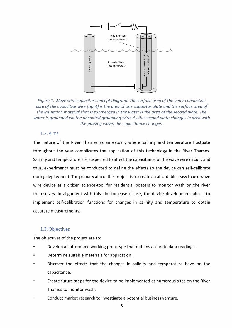
Figure 2. Voltage response on an RC circuit with respect to time in units of the number of time constants. At time t = τ, the voltage always equals 36.8% of the initial voltage.
The time constant of the system can be useful when evaluating the response of a system.
Using Equation 5 during discharge of the capacitor, when time, t, equals the time constant,
the voltage across the capacitor is equivalent to 36.8% of the initial voltage of the system
(Alexander, 2013). For an RC circuit with a set voltage and resistance but with an unknown or
varying capacitance, like the wave wire method, the time to reach 36.8% of the initial voltage
can be measured and then divided by the resistance of the circuit to obtain the capacitance.
As the capacitance changes with the waves, the time constant and steepness of the voltage
response curve shown in Figure 2 will change.
Although other methods can be used to measure capacitance such as phase lag, the time
constant measuring method is used in this project.
1.5.2. Wash Generation Overview
Wave wash generation is caused by the volume displacement of water from the hull of a
passing vessel. During this displacement, not only relatively high-amplitude, high-frequency
waves are generated, but also a set of low-frequency, low amplitude waves. The high-
amplitude waves, known as Kelvin waves, are divergent and transverse waves caused by the
surface interaction of the bow and stern of the vessel. The low-amplitude waves are referred
to as Bernoulli waves explained by Bernoulli’s equation in that there is a rise and fall of the
local water level generated by the balance of the pressure distribution of the vessel hull and
the velocity pattern of the water column. These Bernoulli waves are insignificant in large
bodies of water, but in rivers, estuaries and bay inlets, these waves can cause water excitation
for extended periods of time. Additionally, the initial movement or acceleration of a vessel,

13
known as a drawdown, produces the largest local water level drop that initiates water level
oscillation (Garel, 2008).
Water particles in a wave experience cyclic motion, changing in height and velocity at each
position on the wave surface. At the peak of the wave, the particle velocity is in the direction
of the wave; at the trough, the particle velocity is opposite the wave. With this concept, the
wave possesses and the particles experience both potential and kinetic energy. The elevation
of the water level induces the potential energy while the kinetic energy is due to the cyclic
motion. The total energy of a wave is the sum of the potential energy, Ep, and kinetic energy,
Ek, and for a sinusoidal wave, these two energies are equivalent as shown in Equation 7 where
Etotal is the total energy per unit area of a wave. Here, ρ is the density of water, g is the
acceleration of gravity and ζ is the instantaneous wave amplitude (Giles, 2017).
𝐸𝑡𝑜𝑡𝑎𝑙 = 𝐸𝑝 + 𝐸𝑘 = 1
4 𝜌𝑔𝜁2 +
1
4 𝜌𝑔𝜁2 =
1
2 𝜌𝑔𝜁2 (7)
Equation 7 shows the influence that wave amplitude has on the energy the wave carries, which
shows the importance for monitoring the wave height and profile. This monitoring is beneficial
for residential boaters in calculating the damaging and disrupting energy transferred to their
vessels, but also can be beneficial to energy companies to investigate the potential for
renewable energy in specific areas on the water.
1.5.3. Environmental Impact
As discussed in the project background, the purpose of this project is to develop an accessible
wave wash monitoring system for the River Thames residential boating community; however,
wave wash also has great impact on the river ecology including harmful effects to animal
spawning grounds and habitats as well as increased sediment suspension and erosion of the
river banks.
The Department of Freshwater Ecology at the University of Vienna studied the effects of vessel
wash on three shoreline structures which are main spawning grounds in the Austrian Danube
River. Riverine fish nurseries are normally made in shallow warm waters on the banks with
water depth from 0 to 40 cm. The study of wash and splash from various river vessels showed
that wash can drastically displace microhabitats and nurseries. The studies revealed the
average and maximum drawdown water levels of vessels to be 0.14 and 0.44 m which resulted

14
in 0.66 and 2.08 m shoreline shift respectively. This wash not only causes displacement of
nurseries, but also causes sudden increased currents that interfere with the natural swimming
patterns of fish (Kucera-Hirzinger, 2009).
Additional harm to aquatic animals can occur through suspended solids and silt in the water
caused by the stirring of bank floor sediment by wash and drawdown. Increased suspended
silt in inhabited aquatic environments causes clogging of respiratory structures, reduction in
feeding rates, disruption in mating and spawning behaviour as well as a decrease in fish
hatching rates (Mosisch, 1998).
The University of the Aegean conducted a study of the wave wash generation of conventional
and high-speed ferries for coastal waters. In this study, wave height and duration was
recorded as ferries passed a nearby beach into port. The study concluded that the high-speed
vessel produced wash with significantly higher amplitudes and energy than that of
conventional speed ferries as well as that expected to be generated from the wind wave
regime of the area. The largest wave generated was approximately 0.74 m in amplitude where
waves generated by the wind were generally below 0.1 m in amplitude. The study also stated
that the deep drafted vessels can cause damage and disturbance to coastal structures, benthic
ecosystems and moored and berths vessels (Velegrakis, 2006). An additional study reports
that drawdowns resulting from the quick departure from and arrival into ferry ports produce
much higher potential for sediment resuspension to occur and thus erosion. Sufficient
evidence was obtained to set regulatory measures for vessel speed (Garel, 2008).
Moreover, an in-depth, five-year study of bank erosion on the Gordon estuarian river in
Tasmania, Australia showed that increased regulation of river traffic speeds greatly reduced
bank erosion on the estuary (Bradbury, 1995). With the establishment of a speed limit of 9
knots for all vessels, the erosion rate of the banks reduced from 210 mm per year to 19 mm
per year. Further up the river, commercial cruise vessel traffic was prohibited and the rate of
bank erosion fell from 11 mm to 3 mm per year. Because of the drastic change in erosion rates
in this study, the speed limit was further reduced to 6 knots to further prevent human-induced
harm to the river ecology.

15
Based on the discussed compelling issues and studies, the expansion of the monitoring of
unnatural aquatic surface activity, such as the efforts of this project, can influence the
implementation of reasonable regulation in efforts to reduce harmful effects to the aquatic
environment as well as reduce damage cost for ports, marinas and residential vessels.

16
2. Design Criteria
The development of the initial concept of this wave wire device stemmed from the project
brief, the outlined project objectives in the introduction as well as the previous technology
deployments referenced in the literature review. Through the initial research of this
technology, the following design criteria was outlined as shown in Table 1.
Table 1. List of design criteria.
Design Criterion Notes
Measuring accuracy Design a system to measure wave height with <10% error or 6 mm to the actual wave height from the water surface.
Self-calibration with temperature and salinity
Develop a design that includes temperature and salinity calibration.
Affordability Minimise the overall cost of the device while balancing accuracy capabilities.
Marine environment suitable
Select materials that will withstand the harsh marine environments for long durations of time.
High measuring rate Select electronic components that will allow a suitable measuring rate to capture wave profiles.
Low power consumption Incorporate components with low power consumption, as the device will be battery powered.
Compact Reduce the spatial volume of the device; considering the various deployment locations such as residential piers, marinas, and wildlife reserves.
Manufacturability Ensure ease of manufacturing for the product; aligning with the affordability criteria.
The accuracy of the measured waves is the primary criterion that must be obtained. An
accuracy of less than 10% was selected in accordance with the categorisation of the River
Thames which states that the river wave heights are not to exceed 1.2 meters peak to trough
at any time (Maritime and Coastguard Agency, 2003). A reasonable accuracy goal for wave
monitoring purposes for the first prototype was set within 6 mm height error from the water
surface. The evaluation of this criterion is set to be done through the testing of the prototype
in the wave generation tank in the UCL Roberts Building fluids laboratory.
In accordance with the measurement accuracy, the design of the device should consider the
effects of temperature and salinity on the measurements. The evaluation of this criterion
includes field measurements of the temperature and salinity ranges of the River Thames and
static water depth tests of varying temperature and salinity.

17
Affordability was set as a design criterion for the stakeholders of this project: the residential
boating community, the UCL Engineering Exchange and potentially marinas, public boat
launching sites and wildlife reserves. The evaluation of affordability involves the comparison
of the projected device cost against existing wave gauge costs.
The remaining criteria determine the development of the prototype. Therefore, the
evaluation of the criteria involves the material and component selection. All materials must
be suitable for the harsh marine environment both for functionality and durability. This device
should be designed for long-term deployment with minimal maintenance requirements.
Regarding the capturing of the wave profiles, high measuring rates are required. The
electronic devices selected must have this capability while also maintaining low power
consumption.
The size of the device should be practical for stakeholder use, and the limitation of space on
piers and vessels must be considered. While little evaluation will be made on this subjective
criterion, the design volume will be kept to a minimum.
Manufacturability directly correlates with the device affordability and material selection. Ease
of manufacturing will reduce personnel and fabrication costs as well as production lead time.
Standard materials, hardware and manufacturing processes will be selected for the
development of the device.
18
3. Design and Prototyping
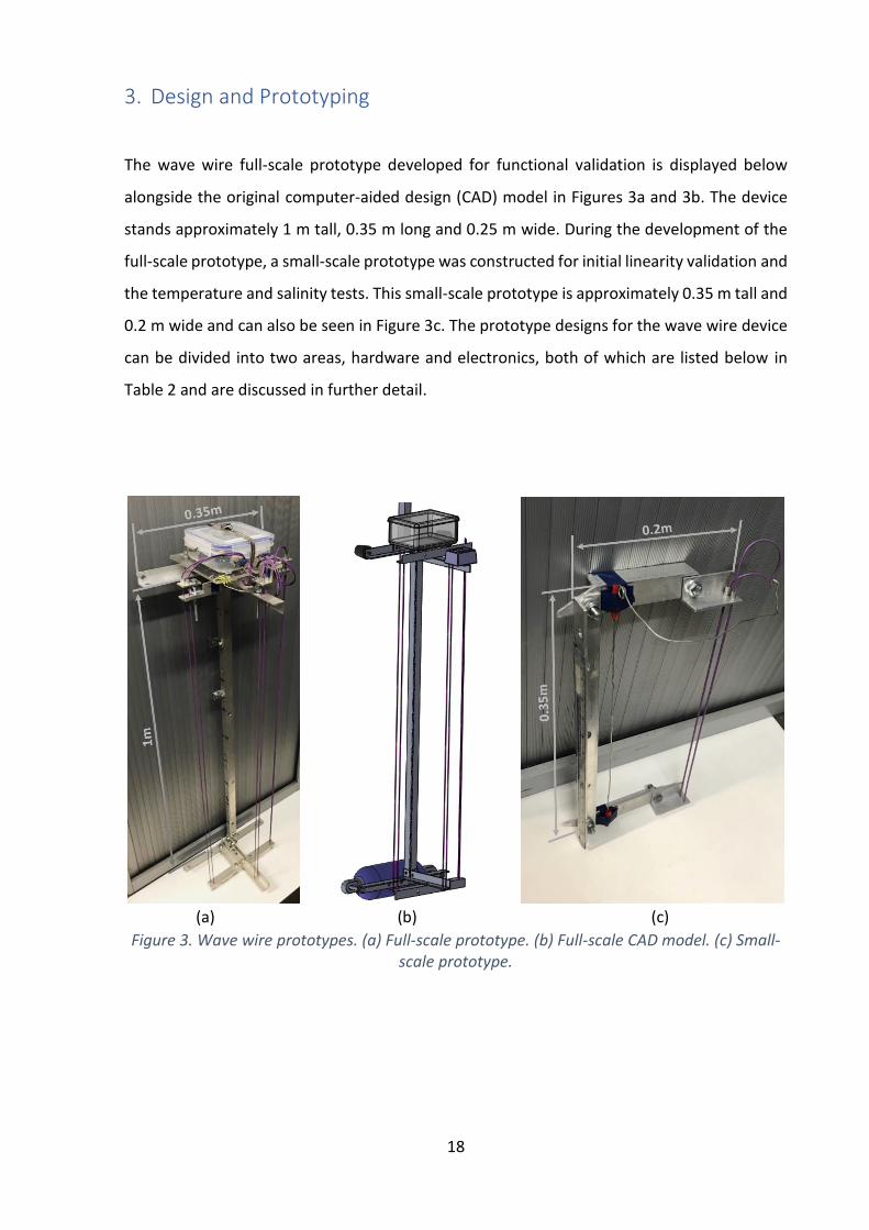
The wave wire full-scale prototype developed for functional validation is displayed below
alongside the original computer-aided design (CAD) model in Figures 3a and 3b. The device
stands approximately 1 m tall, 0.35 m long and 0.25 m wide. During the development of the
full-scale prototype, a small-scale prototype was constructed for initial linearity validation and
the temperature and salinity tests. This small-scale prototype is approximately 0.35 m tall and
0.2 m wide and can also be seen in Figure 3c. The prototype designs for the wave wire device
can be divided into two areas, hardware and electronics, both of which are listed below in
Table 2 and are discussed in further detail.
(a) (b) (c)
Figure 3. Wave wire prototypes. (a) Full-scale prototype. (b) Full-scale CAD model. (c) Small-scale prototype.
19
Table 2. Prototype components and materials list.
Item Use/Description Supplier H
ard
war
e Aluminium
6082-T6 Angle Stock
Device frame material, 1 x 1 x 0.125 in, 5m Farnell
Bolts Fasteners, 8M and 6M stainless steel Screwfix
Nuts Fasteners, 8M and 6M stainless steel Screwfix
Washers Fasteners, 8M and 6M stainless steel Screwfix
Acrylic plate Mounting platform, 30 x 30 x 1cm acrylic plate
IOM
Tupperware container
Electronic housing and waterproofing, 12.5 x 12.5 x 6 cm container
Tesco
Pipe band Electronic housing fastening, 400mm pipe band
DIY
Capacitive wires Multi-stranded, PVC insulated, 22 AWG, 0.5 mm²
Farnell
Grounding wire Tinned copper, 3.1mm2 IOM
Ele
ctro
nic
s
PCap02a evaluation
board
Capacitance-to-digital-converter, wire capacitance sensing
Mouser Electronics
Arduino Mega Microcontroller, master computational system to drive PCap02a board and log data
n/a
Accelerometer Adafruit MMA8451 3-axis accelerometer RS Components
70-piece jumper wires
Circuitry Active Robots
Breadboard Circuitry Active Robots
PCap02a battery 3V lithium battery Mouser Electronics
Arduino battery 5V portable battery Personal
MicroSD card module
SD card data storage Amazon
3.1. Hardware Design
3.1.1. The Frame
The hardware of the prototype is comprised of the structural materials, fasteners, capacitance
and grounding wires, as well as the waterproof encasement for housing electronics.
Aluminium 6082-T6 angle bar extrusion was selected for the structural framing due to the
material’s corrosion resistance in aquatic environments, mechanical strength and

20
affordability. The aluminium frame is assembled out of 5 meters of this angle extrusion and
fastened with 8M nuts and bolts.
The frame geometry was designed as a slim profile to reduce dragging forces induced by the
movement of water. The upper and lower portions of the frame are in a cross configuration
to mount the capacitive wires equidistant from the central grounding wire and to reduce the
materials needed for functionality. The detailed drawing and dimensions of the prototype can
be found in the appendix.
3.1.2. The Wires
The capacitive wires are multi-stranded, copper wires insulated by a PVC polymer coating. The
inner copper core is approximately 0.83 mm in diameter and the PVC outer diameter is
2.38mm. The PVC insulating material of the wire has a dielectric constant of 3.2. Using
Equation 1 with these dimensions and properties, the capacitance of the wire is approximately
158.1 pico-farad (pF) per meter of submerged wire.
The capacitive wires are set up in a double pass apparatus where the wire travels from the
evaluation board down into the water and back up to the board to eliminate the termination
of an electrical wire under water. Wire materials that have been used by previous developers
of wave wire devices include polytetrafluoroethylene (PTFE) coated multi-stranded copper
wires, oxide layer coated tantalum wires, and formvar-enamel coated wires (Pascal, 2009)
(Chapman, 1993) (Killen, 1952). The PVC insulating material is most similar to the PTFE coated
wire and was selected due to affordability, availability and hydrophobic characteristics which
resist material degradation and fouling due to the marine environment, as well as the
capacitance to length ratio calculated from Equation 1.
A wire tightening system was implemented to ensure the capacitive wires were held in tension
and not drastically deflected by the drag force of the water movement across the wires.
Inconsistent wire movement could result in increased uncertainty and measurement error.
The wire tightening system can be seen in Figure 4 below and is made up of the aluminium
extrusion, 6M x 100 mm bolts, aluminium wire crimps, and locking and wing nuts. The wing
nuts enable the wires to be tightened by hand during deployment if they were to lose tension
over time.

21
Figure 4. Visualisation of capacitive wire tension system.
3.1.3. Electronics Encasement
The final portion of the hardware design is the electronic housing, which must be
waterproofed to be deployed in the marine environment. For affordability, a simple
Tupperware container was used to shield the electronics from the weather and aquatic
environment. During the concept generation of the design, maintenance of the device was
evaluated and determined to entail capacitive wire replacement, battery replacement and
device cleaning from any fouling occurring. The connection of the wires to the circuit alongside
the waterproofing the electronics required external ports to protrude from the electronics
housing, which was executed using male wire termination tips that were mounted through
the Tupperware wall and sealed using hot-melt silicon adhesive. The container resulted in no
leaks when held underwater. More detailed photos of the prototype can be found in the
appendix.
3.2. Electronics Design
The electronic system is the core of this device and the system schematic can be seen in Figure
5 below. The design was structured around four of the design criteria: measurement accuracy,
high measurement rate, low power consumption and affordability. The following sections
break down the major electronic system components and functions.
22
Figure 5. Wave wire electronic system schematic. The Arduino Mega is the master device that
communicates with the PCap, MMA8451 accelerometer and micro SD module via I2C communication.
3.2.1. Capacitance Measurement
The data generation system selected is the PCap02a evaluation board (PCap) which is a printed
evaluation board centred around a capacitance-to-digital-converter (CDC) chip. This
evaluation board was selected due to its high measurement rate capabilities, low power
consumption, and high measurement resolution. The PCap is capable of a cycle rate of 50kHz
and a minimum current consumption of 2.5 µA at an operating voltage of 3V. The power
consumption and resolution vary with configuration setpoints, which will be discussed in the
configuration set points subsection. Regarding the electronic hardware, the PCap is capable
of connecting six wave wire sensors for CDC measurements with the additional capability to
measuring temperature using a thermistor (AMS, 2014).
The CDC measurement of each sensor is executed by capacitor discharge time using known
internally set discharge resistors, as well as a known reference capacitor. The time constant
for the reference capacitor is taken in sequence before the capacitive sensor and a ratio of the
time constants is given. With the internal resistors at set equal values, the time constant ratio
and the capacitance ratio of the sensor to reference capacitance are equivalent. The sensor
capacitance can then be calculated with the known reference capacitor value.
The reference capacitor has a capacitance of 47 pF and the PCap can compute ratios up to a
value of eight due to bit size restrictions. This means that the range of capacitance of the wires

23
must be 0 to 376 pf. Using Equation 1, an acceptable range for the PVC insulated wires was
calculated to be 0 to 306 pf.
3.2.2. Configuration Setpoints
The configuration of the PCap determines the power consumption and accuracy of the
capacitance measurement. The key setpoints for CDC operation are the cycle rate, measuring
rate and discharge resistors, which are 50 kHz, 12.5 Hz, and 10 kΩ respectively. The cycle and
measuring rate highly effect the power consumption and noise level. The 50 kHz cycle speed
was selected as it is the PCap pre-determined low-power mode and the measuring rate was
determined to be a minimum while still capturing data quickly enough to obtain readable
wave profiles. With these configurations, the noise reported by the manufacturer should be
in the 20 to 30 aF range and only consuming 16 to 17 µAh (AMS, 2014).
3.2.3. Microcontroller and Data Computation
The computational board chosen was the Arduino Mega 2560 microcontroller. The
communication interface between the Arduino and the PCap, as well as with the implemented
MMA8451 three-axis accelerometer, is I2C communication. The interface uses serial
communication which reads and writes from a master device, the Arduino, to single or
multiple slave devices, the PCap and the MMA8451. I2C interface uses two ports for
communication, a serial clock (SCL) port and serial data (SDA) port. These ports for each device
are all connected, simplifying circuitry wiring.
For PCap operation and data reading, the microcontroller must initially write an operation
command to start the CDC conversion and then read the data from each wave wire port in
sequence. Each port is 24 bits in size, which poses a problem for the eight-bit reading
capabilities of the Arduino. To solve this problem each port must read in eight-bit increments
from three different registers individually. The 24-bit data obtained from each port is
presented to the microcontroller as digitally converted hexadecimal values. Additional math
must be executed regarding the coding loop to combine these three individual bytes of data
into one capacitance ratio which can then be converted into wave height. The complete code
run by the Arduino can be found in the appendix.

24
The communication involved with the MMA8451 accelerometer is similar, but a
preconstructed Arduino library performs the math conversion and provides the device
acceleration data. This acceleration is further processed to approximate velocity and speed
using principle acceleration, velocity and position equations.
Different options were considered for the most appropriate deployment locations for the
device. The side of floating vessels or floating piers appeared to be the practical deployment
option to obtain the most wave measurements with changes in tide. This form of deployment,
however, causes vertical movement of the wave device with respect to the average water line.
The inclusion of the accelerometer eliminates this vertical movement, so wave heights are
truly represented in the final data.
These measurements from the PCap and the MMA8451 are all compiled to a text file that is
logged on a microSD card using the microSD module. This module was selected due to the
ease of functionality to log data straight to an SD card without need for special configuration
of the SD card.
The Arduino is the “master device” that controls all the components previously mentioned
and thus has the highest power consumption at 0.2Wh (40mA at 5V) (Arduino, 2017).
Although this power consumption limits long term deployment, for the initial prototype, the
Arduino was selected due to affordability, availability and the large quantity of development
resources to construct a functioning prototype. A portable battery at a 5V level with 2.2Ah
capacity is provided for the Arduino. Further investigation of low power microcontrollers
should be completed for long term deployment of this device.

25
4. Experiment and Testing Setup
The experimental efforts of this project can be divided into three separate sections: field
measurements, laboratory experiments and field testing. Each section will discuss in detail the
purpose of efforts and testing set up.
4.1. Field Measurements
To investigate the effects that salinity and temperature have on the capacitance wave
measurement method, the fluctuating salinity and temperature ranges of the Thames estuary
were measured throughout the summer months to develop a working range for laboratory
experiments. The equipment used for obtaining these measurements was the HI-98195 multi-
parameter meter logger.
Measurements of the river were taken in three different locations along the River Thames in
west London at Oyster Wharf, central London at Blackfriars Bridge and east of Canary Warf at
Trinity Buoy Warf. Two- to three-hour samples of the incoming and retreating tide were taken
at each location. The salinity measurements obtained were then compared to a report
produced by The City of London Port Health Authority in 2007 that compiled two years of
temperature and salinity data. The ranges represented in the report compared to those
gathered through the river measurements were similar. Therefore, the measurements from
the 2007 report containing full-year temperature ranges were used for the experiment to
include winter temperatures that could not be captured within this project. Salinity and
temperature ranges utilised for laboratory experiments were 0.5 to 5 parts-per-thousand
(ppt) and 5ºC to 25ºC respectively (Lane 2007).
4.2. Laboratory Tests
The tests performed in the laboratory included initial small-scale prototype tests, varying
salinity and temperature tests and final large-scale prototype tests.
For the initial small-scale prototype tests as well as the salinity and temperature variation
tests, the miniature wave wire prototype was used. This small-scale prototype eliminated the

26
need for large testing tanks for the initial functionality validation as well as reduced the
amount of salt and ice needed to varying salinity and temperature.
The initial functionality tests were performed to verify that the selected wire materials would
produce linear results with water depth as well as operate in the capacitive range specified by
the PCap. These initial tests were static tests which measured the capacitance of the wires as
the miniature prototype was lowered into the water in increments of 2 cm. The depth range
that was tested was from 8 cm to 18 cm of submerged wire. The capacitance was measured
using the PCap as well as a resistance-inductance-capacitance (RLC) meter to compare
measurements from different devices to the theoretical capacitance. These tests were run
multiple times to determine the consistency of the measurements against potential
experimental errors such as inaccuracy of water depth which was set using a ruler attached to
the miniature prototype.
The testing for the varying salinity and temperature tests was set up identically to the initial
functional tests with the inclusion of materials in the tank. The material used to increase the
salinity of the tank was Instant Ocean, a sodium compound which mimics actual materials in
brackish and sea water. Two salinity tests were performed. The first test investigated the
effect on capacitance by applying the salinity range that was measured from the River Thames
in increments of 0.2 ppt. The second test was similar but investigated a larger range of salinity,
ranging from fresh water to sea water in increments of 10 ppt to determine whether a drastic
difference in salinity would affect the capacitance measurements. To vary the temperature,
ice was added to the tank, reducing the temperature to 5ºC; hot water was then added to
increase the temperature to 25ºC in increments of 5ºC.
The final laboratory experiments involved the large-scale prototype design and the wave
generation tank in the UCL fluidics laboratory. The large-scale prototype was initially tested
statically, measuring capacitance with respect to submerged wire length from 0 to 90 cm
depth in increments of 10 cm. These static measurements were made to compare the linearity
of the large- and small-scale prototypes while obtaining calibration equations for the large-
scale prototype. Multiple runs of this test were performed to evaluate experimental error and
capacitance variance.

27
Following static testing of the large-scale prototype, dynamic wave tests were run in the wave
generation tank. The wave generation system is a 20 m long tank with oscillating paddles that
generate the waves at one end of the tank and a beach that absorbs the waves at the end of
the tank so minimal wave reflection is made at the end of the tank. The system was set to
generate simple sinusoidal waves with variation in amplitude and frequency for each run. The
ranges of amplitude and frequency were 3, 4 and 6 cm amplitudes and 0.6, 1 and 1.4 Hz. These
ranges were selected based on the typical frequency range of vessel wash waves (0.2 to 1 Hz)
and the capabilities of the wave generation tank system (Tan, 2012). The PCap was used to
measure and log the capacitance during the dynamic tests, and an HD GoPro camera was used
to record each run. A ruler was attached to the glass wall of the wave tank, so the actual wave
heights could be referenced by the video recording during the evaluation of the test capacitive
data.
4.3. Field Tests
After the completion and evaluation of the laboratory tests, the prototype was tested twice
on the River Thames at Oyster Wharf Pier in west London for final prototype testing including
capacitance, acceleration and temperature measurements. The prototype was mounted to
the floating pier so wave height measurements could be taken with the rise and fall of the
tide. The device faced the open river to prevent obstacles from disrupting the wave form of
the wash.
As the wave measurements were taken, each passing vessel type was recorded along with the
time the vessel wash hit the pier to examine wash timings and potential spikes in the data
upon evaluation. The multiparameter meter also logged temperature and salinity during this
test for correct calibration of the device. During the first river test, the capacitance
measurement was collected through the Arduino and printed to the serial monitor on the
connected PC. The data was collected to the PC as datalogging to the SD card was not fully
configured at the date of the first river test. However, the data logging for the final river test
was completely remote with successful datalogging to the SD card and the system running on
battery.

28
5. Results
5.1. Laboratory Experiment Results
5.1.1. Small-Scale Prototype Testing
The initial testing of the small-scale prototype resulted in a purely linear capacitance trend
with respect to submerged wire depth. The prototype was measured using both an RLC meter
and the PCap which both responded with linear trends but yielded different results as seen in
Figure 6 below.
Figure 6. Initial small-scale prototype testing results. RLC is represents the measurements
taken by the Resistance-Inductance-Capacitance Meter. PCap represents the measurements taken by the PCap. Theo represents the theoretical measurement obtained from Equation 1.
PCap shows higher accuracy of only 8.01% error.
The theoretical capacitance shown was calculated using Equation 1 with the actual dimensions
of the wire and a PVC dielectric constant of 3.2 as well as the actual submerged length of the
wire (National Physical Library, 2017). In comparing the two devices to the theoretical trend,
the PCap is more accurate with respect to the gradient, yielding a percent error of 8.01% as
opposed to the 54.07% from the RLC meter. This error from the Pcap could be a result of
inconsistent thickness of the dielectric coating in addition to experimental error when setting
the depth of the device while taking measurements. Manufacturing tolerances were
researched for the PVC wires but such specifications are not published by the manufacturer.
The vertical shift of the trend line is a reproducible systematic error of stray capacitance of
the prototype, i.e. the capacitance of the wires without submersion. Ideally, this capacitance
would be zero; however, internal capacitance in the CDC is unavoidable as well as additional
stray capacitance from the aluminium frame.
The near parallel gradient of the PCap to the theoretical capacitance trend is desired but not
necessary. Since the PCap capacitance trend with respect to water depth is linear, the

29
measurements can be calibrated and directly translated regardless of the accuracy relative to
the theoretical equation.
The first salinity variation test was conducted over the range of salinity, 0.5 ppt to 5 ppt,
measured on the River Thames throughout the project. The initial results showed salinity had
an insignificant effect on the capacitance, so a second test was conducted over a more
extreme range, spanning from brackish water salinity, 5 ppt, to typical oceanic salinity, 35 ppt,
in 10 ppt increments. The results of this test were similar to the initial test, so best-fit
trendlines were given to each salinity data set and were extrapolated to better examine the
deviations as shown below in Figure 7. The temperature in these tests was relatively constant
with a minimal decrease from 25.02°C to 24.49°C as the salinity was raised from 5 ppt to 35
ppt.
(a) (b)
Figure 7. Salinity variation test. (a) Extrapolated trend line from measured data. (b) Zoomed view of 90 cm to 100 cm depth range. There is no apparent trend of salinity effect on
capacitance measurement as the trendlines are not in sequence. Additionally, there is a maximum deviation of 0.83% across a 700% increase in salinity from 5 ppt to 35 ppt.
There are slight changes in gradient and vertical shifts to the data sets as the salinity varies;
however, there is no apparent pattern in the results shown in Figure 6b above. The 15 and 25
ppt data sets are out of sequence, revealing that fluctuation in salinity does not have a direct
effect on this capacitive measuring method. The largest deviation of these data sets was 2.86
pF between the 35 and 5 ppt points at a 100 cm depth, approximately a 0.83% deviation.
The temperature variation tests created more crucial results for determining the design of the
device. The change in the capacitive gradient can be observed in Figure 8 below. As the
temperature increased in increments of 5°C, the capacitance-water depth gradient increased

30
by approximately 5.56% on average. The y-intercepts of the trendline equations have minimal
shift with a standard deviation of 0.53 pF with a mean intercept of 10.41 pF.
Figure 8. Temperature variation test results show increase in capacitance by 5.56% on
average per 5°C increase.
5.1.2. Large-Scale Prototype Testing
After investigating the salinity and temperature parameters, the final prototype was statically
tested for calibration with water depth in increments of 10 cm. The capacitive trend for each
wire remained linear over the large range of depth with slightly smaller gradients from the
small-scale prototype as seen in Figure 9. There was a significant increase in vertical shift due
to increased stray capacitance. This increase is expected as the wires are more than tripled in
length from 95 to 285 cm. The stray capacitance shift resulted in an average 16 pF increase.
Figure 9. Large scale prototype static test calibration. Results still show linearity, but an
increased shift in stray capacitance of 16pF on average.
This calibration test was conducted in the wave generation tank just before the dynamic
testing occurred with a constant temperature of 24.05°C. The dynamic wave testing included
15 runs with varying amplitudes and frequencies of the wave generation setpoints. In-depth
analysis of three out of the 15 runs was conducted, analysing runs with frequencies of 0.6, 1,
and 1.4 Hz, at an amplitude setpoint of 4 cm. This analysis involved converting the raw

31
capacitance measurements into wave heights using the calibration curves in Figure 9 and
comparing the measurements to the data from the video footage. A breakdown of the 1 Hz
run results can be seen below in Figure 10.
Figure 10. Dynamic functional test results, full-scale prototype. 1Hz wave Generation. (a) Complete run - 60 second, 35 second of waves. (b) Relative zero shift – 15 to 60 second
period. (c) Stabilised waves – 35 to 45 second period. (d) Stabilised waves, wire 2 only – 35 to 45 second period. Results show an average percent error of 8.89% for the three wires.

32
In Figure 10a, the initial 22 seconds of the test are measurements of an idle tank to capture a
zero-baseline reference point. Within this period, the wave generation system was activated
and waves reached the wave wire device after 23 seconds. In analysing Figure 10a, as
generated waves pass, the average water level, i.e. the level at phases 0° and 180° of the
sinusoidal wave, slightly shifts vertically, approximately 1 cm. This shift is a reoccurring
systematic error and is suspected to be caused by the paddles that generate the waves in the
tank, creating a more positive displacement in the tank than negative. To compensate for the
vertical shift, an average of all the data points from the passing waves was taken for each wire
and subtracted from the original data. This shift can be seen in Figure 10b where the sinusoidal
waves have been centered to zero.
Additionally, in Figure 10b, the actual wave heights plotted using the video footage can be
compared to the wire measurements. Error bars have been added to the video generated data
with a value of ±0.5 mm due to experimental error with the uncertainty of ruler
measurements. Additionally, the waves seemed to stabilise at about 35 seconds where the
generated waves started hitting the beach at the end of the wave tank. The measured wave
heights show promising results for accuracy with the video plotted actual wave heights and
can be further examined in Figures 10c and 10d.
In the data displayed in Figures 10c and 10d, the average percent error for wires 1, 2, and 3
are 10.65%, 7.54%, and 9.95% respectively, as shown in Table 3 below, with additional percent
error data from all three runs. The wave curve data from the 0.6 and 1.6 Hz runs can be seen
in the appendix in the same format as Figures 10a through 10d.
Table 3. Percent error statistics for wave generation tests with varying frequency.
0.6 Hz
10 Wave Peaks
1 Hz
19 Wave Peaks
1.6 Hz
26 Wave Peaks
Wire 1 Wire 2 Wire 3 Wire 1 Wire 2 Wire 3 Wire 1 Wire 2 Wire 3
Average % Error 6.72% 8.98% 10.96% 10.65% 7.54% 9.95% 40.18% 44.80% 18.94%
Max % Error 14.86% 13.02% 23.50% 29.83% 39.74% 25.92% 79.04% 151.79% 37.81%
Min % Error 2.03% 5.18% 3.27% 0.09% 0.46% 1.59% 12.02% 6.60% 0.21%
Count >10% Error 3 4 5 9 3 8 26 24 20
33
5.2. Field Test Results
The field tests on the River Thames were simple functional tests to examine if the device shows
definitive spikes in capacitance as vessels generate large wash. For the two tests, the
prototype was launched and intended to log data for two hours. However, obstacles arose
when intermittently, the data stopped logging. Although identified quickly, the issue required
the data to be exported and saved before the data logging could recommence. This issue
occurred because of loose electronic wiring as well as the fact that the length of the wires was
too long for the I2C communication. The combination of these two issues resulted in disrupted
communication between the Arduino and the other devices, halting data logging at each
occurrence. Suitable amounts of data were collected regardless of the wiring issues.
A section of the first test can be seen in Figure 11 below. During this period of data collection,
three different vessels passed along the river. The vessels passing were a Thames Clipper (25
m), a Thames Clipper (38 m) and a small rib boat (6 m). The wash from each vessel reached
the pier at approximately 5.5, 13 and 13.5 minutes respectively. The data and wash events are
highlighted in Figure 11 below. It should be noted that these wave height measurements
include the movement of the floating pier. Therefore, these measurements are not actual
wave height measurements but do show spikes at each wash occurrence.
34
(b) (c)
Figure 11. River test 1 results section. Three vessels passing at 340, 780 and 810 second marks. (a) Full test. (b) Focus of Vessel 1 wash. (c) Focus of Vessels 2 and 3 wash.
The second test on the river was completely “hands-free”, meaning the SD card was inserted
into the system, the power was connected and the measurements were logged. The following
data in Figure 12 was collected when two vessels passed. The first vessel was a tour boat (30
m) and the wash reached the pier at approximately one minute. The second vessel was a slow-
moving houseboat (20 m) and the wash event occurred at 3.5 minutes. Both events are
highlighted in Figure 12.
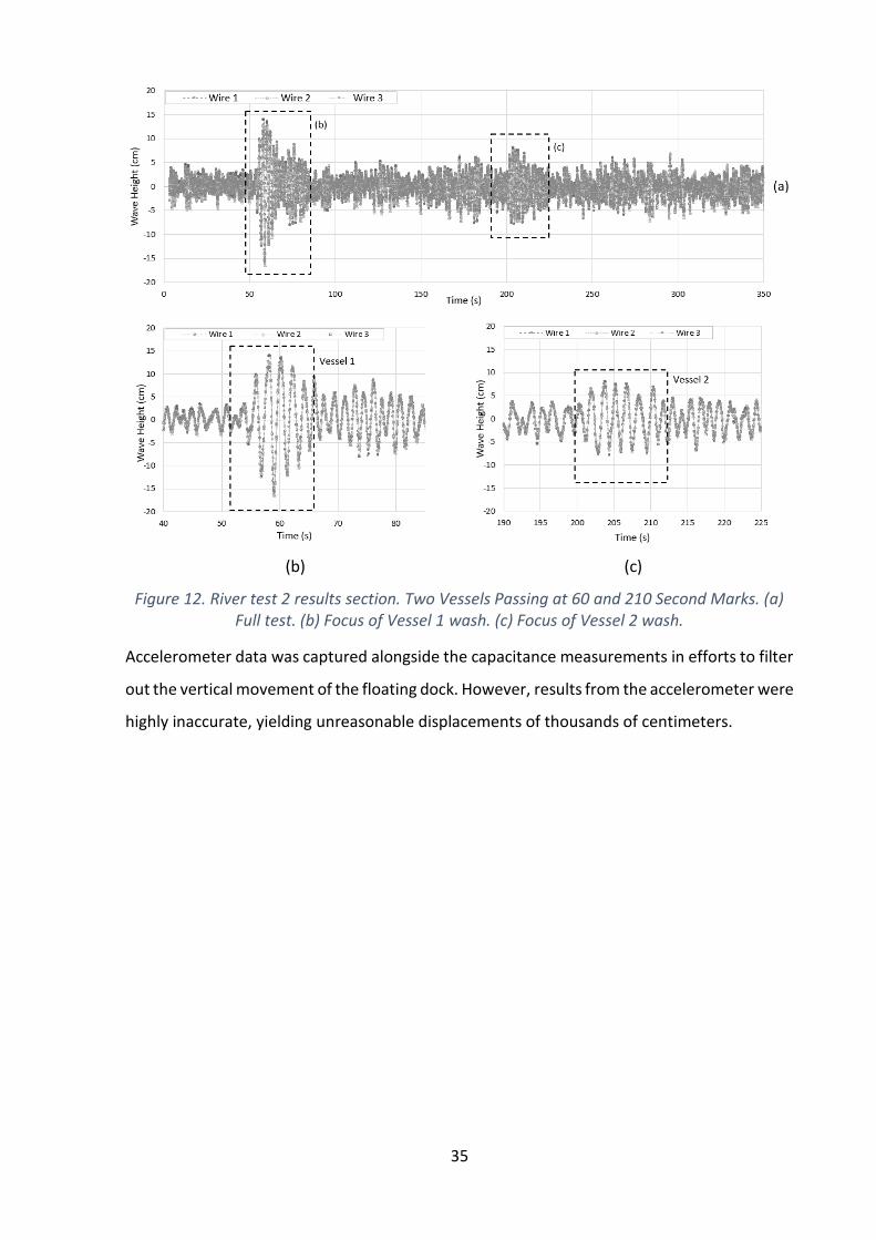
35
(b) (c)
Figure 12. River test 2 results section. Two Vessels Passing at 60 and 210 Second Marks. (a) Full test. (b) Focus of Vessel 1 wash. (c) Focus of Vessel 2 wash.
Accelerometer data was captured alongside the capacitance measurements in efforts to filter
out the vertical movement of the floating dock. However, results from the accelerometer were
highly inaccurate, yielding unreasonable displacements of thousands of centimeters.

36
6. Discussion
The main objectives in designing and testing the prototype were to meet the original design
criteria listed in Table 1. This section discusses the experimental results, prototype
performance against the design criteria as well as future steps to improve the overall design.
6.1. Test Result Discussion
As stated with the results of the salinity variation test, the fluctuation in salinity does not
directly effect this capacitive measuring method. The shifts and deviations shown in Figure 7
are a result of random experimental error in setting the miniature prototype at the specified
measurement depth imprecisely. A ruler was attached to the miniature prototype, and each
water depth was visually set with the waterline against the ruler. Typically, the uncertainty of
a ruler is 0.5 mm. The meniscus of the water on the ruler produced further uncertainty. To
confirm this experimental error, the small-scale prototype was tested a second time at each
salinity, and the data sets again produced no apparent pattern but held tight deviations. Due
to these results, salinity monitoring is unnecessary.
The variation in temperature, however, proves to have a significant effect on the measured
capacitance and thus the measurement of the wave height with the 5.56% increase in linear
gradient per 5°C increase. This result with consistent change in gradient suggests that the
dielectric constant fluctuates linearly with the change in temperature as discussed in the
literature review due movement of dipoles in the microstructure (Srivastava, 1956) (Yadav,
2010). If temperature is not monitored, wave heights measured at 100 cm could vary as much
as 20 cm within the 5°C and 25°C range. The system can self-calibrate with these trendlines if
a simple measurement of temperature is taken alongside the capacitance measurement using
a thermistor connected to the PCap.
The comparison of the percentage error statistics for each dynamic wave test run displayed
in Table 3 suggests the wave wire device has higher accuracy at lower wave frequency. This
result is expected due to the constant measuring rate of 12.5 Hz through all three runs and
thus greater resolution for the lower wave frequencies.
37
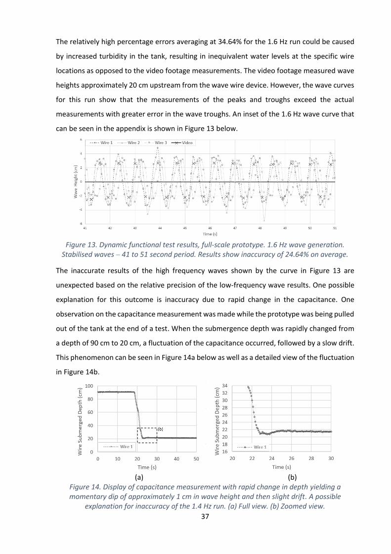
The relatively high percentage errors averaging at 34.64% for the 1.6 Hz run could be caused
by increased turbidity in the tank, resulting in inequivalent water levels at the specific wire
locations as opposed to the video footage measurements. The video footage measured wave
heights approximately 20 cm upstream from the wave wire device. However, the wave curves
for this run show that the measurements of the peaks and troughs exceed the actual
measurements with greater error in the wave troughs. An inset of the 1.6 Hz wave curve that
can be seen in the appendix is shown in Figure 13 below.
Figure 13. Dynamic functional test results, full-scale prototype. 1.6 Hz wave generation.
Stabilised waves – 41 to 51 second period. Results show inaccuracy of 24.64% on average.
The inaccurate results of the high frequency waves shown by the curve in Figure 13 are
unexpected based on the relative precision of the low-frequency wave results. One possible
explanation for this outcome is inaccuracy due to rapid change in the capacitance. One
observation on the capacitance measurement was made while the prototype was being pulled
out of the tank at the end of a test. When the submergence depth was rapidly changed from
a depth of 90 cm to 20 cm, a fluctuation of the capacitance occurred, followed by a slow drift.
This phenomenon can be seen in Figure 14a below as well as a detailed view of the fluctuation
in Figure 14b.
(a) (b)
Figure 14. Display of capacitance measurement with rapid change in depth yielding a momentary dip of approximately 1 cm in wave height and then slight drift. A possible
explanation for inaccuracy of the 1.4 Hz run. (a) Full view. (b) Zoomed view.

38
There is a momentary dip in the capacitance equating to approximately 1 cm at 23 seconds
and then a steady drift over the next 15 seconds. This occurrence potentially explains the
inaccuracy of the 1.6 Hz wave run; however, further research and tests must be done to
investigate this hypothesis.
A possibility for the drift in Figure 14 is delayed water run-off from the wires due to the
adhesion of the water to the wire. Further tests can be done to investigate this hypothesis and
compare water adhesion and run-off of different wire materials.
The accelerometer results that can be viewed in the appendix, indicate that the measuring
rate for the accelerometer was not fast enough to obtain accelerations that would balance in
magnitude. The instantaneous upward accelerations of the dock would be great in magnitude
but this magnitude would not me matched as the dock accelerated downward. With these
uneven accelerations, when the velocity and position changes were calculated through
integration, the resultant displacements drifted to magnitudes of thousands of centimeters,
whereas the vertical movement of the pier typically fluctuated by 2 to 7 cm. Due to the lack
of functionality from the accelerometers, the actual wave heights from the initial river tests
cannot be determined; however, the spikes at the appropriate times for passing wash in
Figures 11 and 12 provide assurance of the device functional capabilities in remote
deployments.
6.2. Prototype Design Criteria Evaluation
The first design criterion, measurement accuracy, required the capability to measure wave
heights to an accuracy within 10% error or 6 mm error for the peaks and troughs of the largest
waves on the River Thames. Based on the dynamic test results in the wave generation tank
and the percent error statistics shown in Table 3, this criterion is met acceptably for the initial
prototype, but improvements can be made. The inaccuracy of the device increases as the wave
frequency increases; however, from the results obtained from the 0.6 and 1 Hz wave
frequency tests, the combined average percent error for the three wires experienced was
8.89% and 9.38% respectively. The lower two wave frequencies are also within the typical
range of wave frequencies generated by wash, 0.2 to 1 Hz (Tan, 2012).

39
The second criterion involved the implementation of temperature and salinity measurements
alongside capacitance measurements. The effects of these parameters result in a capacitance
gradient shift that increases the capacitance measurements by 20% as temperature increases
in increments of 5°C. Salinity showed no apparent trend or direct effect on capacitance. The
PCap provides temperature measurement capabilities through the implementation of a
thermistor, which uses a similar time constant measurement principle as that of the
capacitance measurements where the resistance varies in the RC circuit instead of the
capacitance.
Affordability, balanced with measurement accuracy, was another imperative criterion. For this
prototype, the overall cost was approximately £337. This cost will fluctuate with the
refinement of the device, further discussed in the future steps section. Compared to the costs
of existing wave measurement devices, the relatively low cost of this product shows great
potential for affordability.
Although the materials chosen for the prototype are suitable for the marine environment, the
strength of the frame should be improved. Over the course of the project, as the wave wires
were tightened and loosened, the aluminium frame became slightly distorted. It is suspected
that long exposure to the marine environment could cause significant wear and damage. The
concept for strengthening the frame can be seen in the future steps section.
The electronics selected for the prototype matched the high measurement rate criterion with
the exception of the measuring rate required for accelerometer measurements. The
measuring rate of the PCap has capabilities that could potentially compensate for the higher
wave frequencies; however, higher measuring frequency can affect the dielectric material
properties which would distort the calibration curves generated throughout the project. The
measuring rate of 12.5 Hz was kept constant for this reason.
The PCap also revealed promising results for power consumption, only consuming 16 to
17µAh, which can operate on a 3V-R2032 battery for ideally two years. However, the Arduino,
a limitation for power consumption, operates at 40 mAh. The small capacity battery used for
the prototype was a 5 V, 2.2 Ah battery, so the Arduino could only operate for approximately

40
5.5 hours. This factor does not meet the design criteria, but can be improved for long-term
deployment applications.
Finally, the prototype was designed to be compact and easily manufactured. The overall
volume of the device equates to under 0.1 m2. The manufacturing of the device can be
performed using hand tools. Each component is standardised and can be purchased from any
hardware shop or distributer.
6.3. Future Steps
Overall, the prototype showed promising results for feasibility of the proposed application;
however, further development can refine and improve the short-comings of the device. The
largest area for improvement involves the filtering of movement created by the mounting
point like the floating pier. An accelerometer was implemented as the first potential solution
for this problem, but the sampling rate was insufficient to balance the upward and downward
accelerations. There is also a significant amount of uncertainty when using accelerometers to
measure displacement. If the accelerometer is mounted even a degree off the vertical axis,
the exact acceleration cannot be obtained.
A potential component to replace the accelerometer is a water depth measuring device that
can be attached to the wave wire frame. As the pier and the wave wire device oscillate
vertically with passing waves, the depth measured to the river bed fluctuates and filters the
displacement of the device.
Additional electronic and system updates include a security camera system that takes pictures
up and down the river when a certain wave height threshold is exceeded. This threshold could
be determined by the user or the local authorities in order to assist wash monitoring and
enforcement. The logging system would be developed to stream the wave height data and
photos wirelessly to users.
In order to implement these new components and functions, further work must be done to
reduce power consumption on the computational board and increase battery capacity. The
functions performed by the Arduino on this prototype are simple I2C communications that
41
can potentially be performed on less power-drawing microcontrollers. Renewable sources for
power, such as solar or tidal, will also be investigated but may increase the cost and
compromise the affordability of the product.
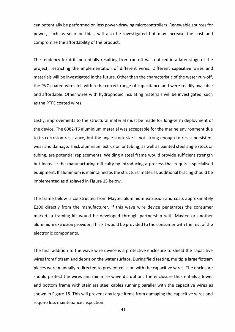
The tendency for drift potentially resulting from run-off was noticed in a later stage of the
project, restricting the implementation of different wires. Different capacitive wires and
materials will be investigated in the future. Other than the characteristic of the water run-off,
the PVC coated wires fell within the correct range of capacitance and were readily available
and affordable. Other wires with hydrophobic insulating materials will be investigated, such
as the PTFE coated wires.
Lastly, improvements to the structural material must be made for long-term deployment of
the device. The 6082-T6 aluminium material was acceptable for the marine environment due
to its corrosion resistance, but the angle stock size is not strong enough to resist persistent
wear and damage. Thick aluminium extrusion or tubing, as well as painted steel angle stock or
tubing, are potential replacements. Welding a steel frame would provide sufficient strength
but increase the manufacturing difficulty by introducing a process that requires specialised
equipment. If aluminium is maintained as the structural material, additional bracing should be
implemented as displayed in Figure 15 below.
The frame below is constructed from Maytec aluminium extrusion and costs approximately
£200 directly from the manufacturer. If this wave wire device penetrates the consumer
market, a framing kit would be developed through partnership with Maytec or another
aluminium extrusion provider. This kit would be provided to the consumer with the rest of the
electronic components.
The final addition to the wave wire device is a protective enclosure to shield the capacitive
wires from flotsam and debris on the water surface. During field testing, multiple large flotsam
pieces were manually redirected to prevent collision with the capacitive wires. The enclosure
should protect the wires and minimise wave disruption. The enclosure thus entails a lower
and bottom frame with stainless steel cables running parallel with the capacitive wires as
shown in Figure 15. This will prevent any large items from damaging the capacitive wires and
require less maintenance inspection.
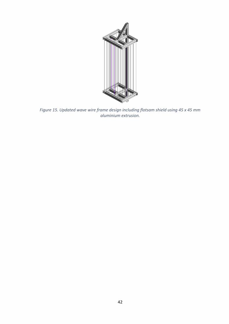
42
Figure 15. Updated wave wire frame design including flotsam shield using 45 x 45 mm aluminium extrusion.
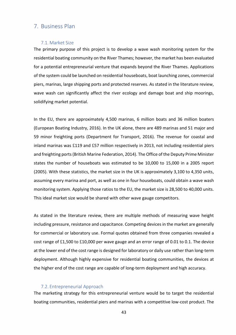
43
7. Business Plan
7.1. Market Size The primary purpose of this project is to develop a wave wash monitoring system for the
residential boating community on the River Thames; however, the market has been evaluated
for a potential entrepreneurial venture that expands beyond the River Thames. Applications
of the system could be launched on residential houseboats, boat launching zones, commercial
piers, marinas, large shipping ports and protected reserves. As stated in the literature review,
wave wash can significantly affect the river ecology and damage boat and ship moorings,
solidifying market potential.
In the EU, there are approximately 4,500 marinas, 6 million boats and 36 million boaters
(European Boating Industry, 2016). In the UK alone, there are 489 marinas and 51 major and
59 minor freighting ports (Department for Transport, 2016). The revenue for coastal and
inland marinas was £119 and £57 million respectively in 2013, not including residential piers
and freighting ports (British Marine Federation, 2014). The Office of the Deputy Prime Minister
states the number of houseboats was estimated to be 10,000 to 15,000 in a 2005 report
(2005). With these statistics, the market size in the UK is approximately 3,100 to 4,350 units,
assuming every marina and port, as well as one in four houseboats, could obtain a wave wash
monitoring system. Applying those ratios to the EU, the market size is 28,500 to 40,000 units.
This ideal market size would be shared with other wave gauge competitors.
As stated in the literature review, there are multiple methods of measuring wave height
including pressure, resistance and capacitance. Competing devices in the market are generally
for commercial or laboratory use. Formal quotes obtained from three companies revealed a
cost range of £1,500 to £10,000 per wave gauge and an error range of 0.01 to 0.1. The device
at the lower end of the cost range is designed for laboratory or daily use rather than long-term
deployment. Although highly expensive for residential boating communities, the devices at
the higher end of the cost range are capable of long-term deployment and high accuracy.
7.2. Entrepreneurial Approach
The marketing strategy for this entrepreneurial venture would be to target the residential
boating communities, residential piers and marinas with a competitive low-cost product. The
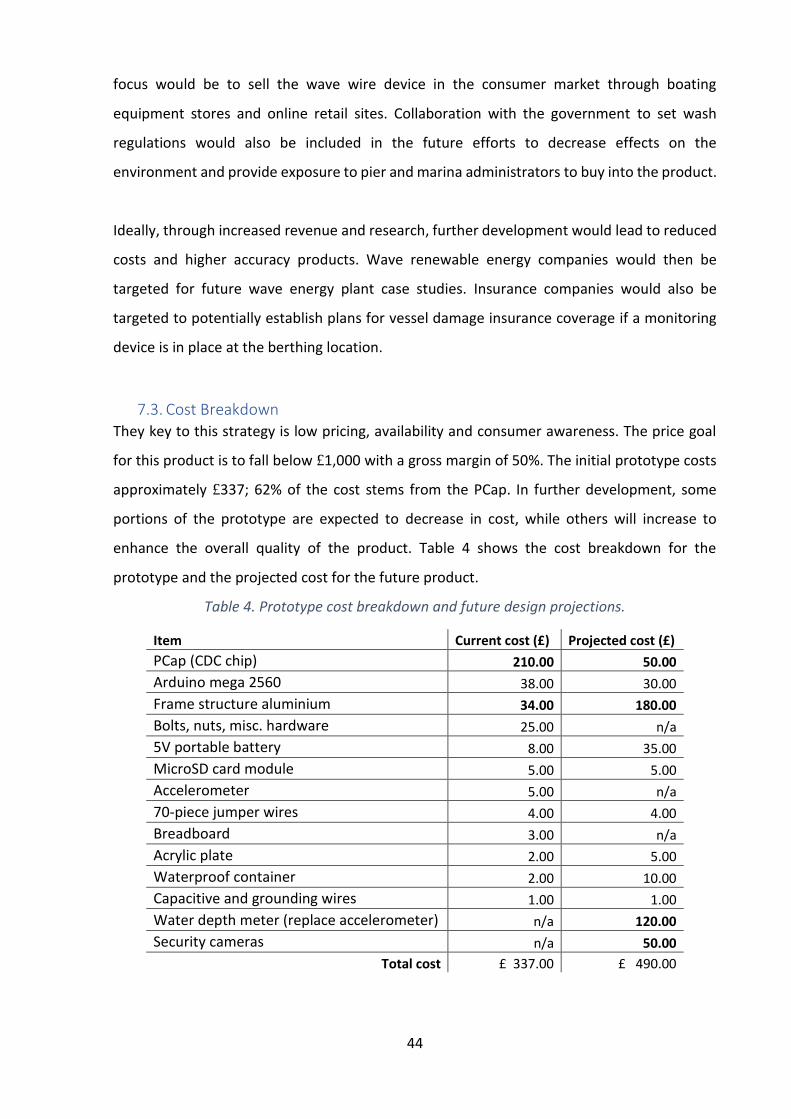
44
focus would be to sell the wave wire device in the consumer market through boating
equipment stores and online retail sites. Collaboration with the government to set wash
regulations would also be included in the future efforts to decrease effects on the
environment and provide exposure to pier and marina administrators to buy into the product.
Ideally, through increased revenue and research, further development would lead to reduced
costs and higher accuracy products. Wave renewable energy companies would then be
targeted for future wave energy plant case studies. Insurance companies would also be
targeted to potentially establish plans for vessel damage insurance coverage if a monitoring
device is in place at the berthing location.
7.3. Cost Breakdown They key to this strategy is low pricing, availability and consumer awareness. The price goal
for this product is to fall below £1,000 with a gross margin of 50%. The initial prototype costs
approximately £337; 62% of the cost stems from the PCap. In further development, some
portions of the prototype are expected to decrease in cost, while others will increase to
enhance the overall quality of the product. Table 4 shows the cost breakdown for the
prototype and the projected cost for the future product.
Table 4. Prototype cost breakdown and future design projections.
Item Current cost (£) Projected cost (£)
PCap (CDC chip) 210.00 50.00
Arduino mega 2560 38.00 30.00
Frame structure aluminium 34.00 180.00
Bolts, nuts, misc. hardware 25.00 n/a
5V portable battery 8.00 35.00
MicroSD card module 5.00 5.00
Accelerometer 5.00 n/a
70-piece jumper wires 4.00 4.00
Breadboard 3.00 n/a
Acrylic plate 2.00 5.00
Waterproof container 2.00 10.00
Capacitive and grounding wires 1.00 1.00
Water depth meter (replace accelerometer) n/a 120.00
Security cameras n/a 50.00
Total cost £ 337.00 £ 490.00

45
The main changes in the future cost structure are shown in bold text in the table. While the
PCap shows promising functionality, it has unnecessary capabilities for a functioning wave
wire product. For the capacitance computation, a self-printed electronics board would be
developed around a CDC chip, around £5. The rest of the cost allotted to the CDC chip includes
manufacturing and circuitry components. The aluminium frame requires increased structural
strength for long-term deployment. This results in a projected cost of £180 with the
assumption of a 10% discount from economies of scale. The future implementation of the
water depth meter and security cameras have been detailed in the discussion section, but are
projected to cost £120 and £50 respectively. The resultant projected cost for the future design
is within the 50% margin goal at approximately £490.
7.4. Financing The funding strategy for this venture would begin with an application for a government grant.
If awarded, a grant would ideally provide funding for the development of the first wave wire
product for at least one year and open communication with the government to implement
new regulations for river areas in the UK. Some available grants available include the European
Maritime and Fisheries Fund (EMFF) and the business innovation fund. The EMFF, established
in January 2016, has a budget of €92.1 million to provide funding for initiatives through 2020
that improve coastal sustainability, the health and safety of fishing vessels and ports and
landing sites (Gov, 2016). The wave wire monitoring device could aid in the health and safety
of fishing ports and berthing zones. The business innovation fund is a competitive fund where
a business or organisation can receive funding between £25,000 and £10 million (Gov, 2017).
Additional funding options would preferably involve a business angel with connections in the
boating and marina industries to increase awareness of the product.

46
8. Conclusion
The purpose and aims of this project are both to develop an affordable, easy-to-use wave
measurement prototype as a citizen science-tool using capacitive wire methods as well as to
investigate the effects of salinity and temperature on the capacitive measurements so the
device can be self-calibrating with the fluctuations in estuarian environments. Through the
construction and testing of two separate prototypes, linear relation between the measured
capacitance and the submerged wire is confirmed and compared to theoretical calculations,
yielding a maximum error of 8.01%.
The investigation proves salinity variation has no significance on the capacitance
measurement for this method. There is no sequential change in gradient or shift in the
capacitance to water depth relation due to salinity change. The largest deviation in
capacitance measurement was 0.83%, which is likely due to random experimental error in the
testing setup.
Noticeable effect on capacitance was observed in the temperature variation tests where the
capacitance to water depth gradient increases by a factor of 5.56% per 5°C temperature
increase. For the system to self-calibrate, a thermistor must be added to measure
temperature alongside the capacitance measurements. This implementation of a thermistor
is a simple addition only requiring soldering of the component to the PCap, calibration tests
and a slight change in microcontroller coding.
The results of the dynamic tests show that the accuracy of the device decreases as the wave
frequencies increase. The objective to achieve measurement accuracy below 10% error was
achieved by two of the three wires during the two lower wave frequency tests and had a
combined percent error of 8.89% and 9.38% across the three wires for the 0.6 and 1 Hz runs
respectively. The results of these two tests show promise for applications in the river
environments to detect wash, due to the standard wash wave frequency range being 0.2 Hz
to 1 Hz (Tan, 2012). The high errors experienced in the dynamic wave test were produced only
when operating outside of this wave frequency range.

47
Field tests on the River Thames proved that detection of wash events is obtainable; however,
filtering of the movement of the floating pier could not be accomplished with the
accelerometer selected. Future steps to improve the current prototype are to replace the
movement-filtering accelerometer with a water depth meter, implement a security camera
system, set up wireless data logging, investigate renewable sources for power, refine the
electronic components to reduce power consumption, add structural updates to protect the
device against damage from the environment and flotsam, as well as add a thermistor to self-
calibrate the wave measurements through temperature monitoring.
There is a potential market for the product, ranging from 28,500 to 40,000 potential units in
the EU marine community alone. Competition that has been observed primarily focuses on
industrial and commercial clients with products that are typically either large robust systems
that are permanently installed or small systems that would be used in the laboratory or for
daily use. A low-cost and easily obtainable device for long-term deployment seems to be
lacking in the market today. A device such as this can encourage boating residents and
authorities to monitor unnatural environmental processes that can cause damage to
residential boating structures and have a detrimental effect on marine ecology.
The efforts herein confirm the ability to construct an affordable, relatively accurate wash
monitoring device that self-calibrates with variation in temperature and can be deployed by
citizens and communities on the River Thames and in other marine environments.

48
References
Alexander C, Sadiku M, 2013. Ch. 6 Capacitors and Inductors and Ch. 7 First Order Circuits.
In: Lange M eds. Fundamentals of Electrical Circuits [online]. 5th ed. New York, NY:
McGraw-Hill, pp. 215-219, 254-257. Available from:
https://s3.amazonaws.com/academia.edu.documents/43400833/Alexander_-
_Fundamentals_of_Electric_Circuits_5th_c2013_txtbk.pdf?AWSAccessKeyId=AKIAIW
OWYYGZ2Y53UL3A&Expires=1504457686&Signature=o2gYMTJgjb3MSrZA%2FuTsKYn
F3gA%3D&response-content-
disposition=inline%3B%20filename%3DElectric_Circuits_FiFth_Edition_Electric.pdf
[Accessed 20 August 2017].
AMS. 2014. PCap02A Single-chip Solution for Capacitance Measurement Volume 1: General
Data and Front-end Description. Unterpremstaetten, Austria. AMS. Available from:
http://www.acam.de/products/picocap/documentation/ [Accessed 16 June 2017].
Arduino. 2017. Arduino Mega. [online] Available from:
https://www.arduino.cc/en/Main/arduinoBoardMega [Accessed 28 August 2017].
Bradbury J, Cullen P, Dixon G, Pemberton M, 1995. Monitoring and Management of
Streambank Erosion and Natural Revegetation on the Lower Gordon River,
Tasmanian Wilderness World Heritage Area, Australia. Environmental Management.
Vol. 19 (2). [online]. pp. 259-272. Available from:
https://link.springer.com/article/10.1007/BF02471995 [Accessed 18 August 2017].
British Marine Federation, 2014. Research Overview – Marinas [online]. Available from:
http://britishmarine.co.uk/~/media/BMF/Files%20and%20Documents/PDF/Statistics
/Marinas%20Overview%202014.ashx [Accessed 1 September 2017].
Broeders J, Pascal R, Cresens C, Waugh E, Cardwell C, Yelland M, 2016. Smart Electronics for
High Accuracy Wave Height Measurements in the Open Ocean. National
Oceanography Centre.
Chapman R., Monaldo F. M., 1993. A Novel Wave Height Sensor [online]. Vol. 12 Journal of
Atmospheric and Oceanic Technology. The John Hopkins University Applied Physics
Laboratory. pp. 190-196. Available from:
http://journals.ametsoc.org/doi/pdf/10.1175/1520-
0426%281995%29012%3C0190%3AANWHS%3E2.0.CO%3B2 [Accessed 16 June
2017].
Department for Transport, 2016. Port Freight Statistics 2016 [online]. pp. 18-19. Available
from:
https://www.gov.uk/government/uploads/system/uploads/attachment_data/file/64
1322/port-statistics-technical-note.pdf [Accessed 1 September 2017].
European Boating Industry, 2016. Facts and Figures [online]. Available from:
http://www.europeanboatingindustry.eu/facts-and-figures [Accessed 31 August
2017].
Garel E, Fernandez L, Collins M, 2008. Sediment resuspension events induced by the wake
wash of deep-draft vessels. Geo-Marine Letters. Vol. 28 (4). [online]. pp. 205-211.
Available from: https://link.springer.com/article/10.1007/s00367-008-0101-y
[Accessed 19 August 2017].
Giles T, 2017. UCL Marine Renewable Energy Lecture 1.

49
Gov.UK, 2016. Information about the available funding from the European Maritime and
Fisheries Fund (EMFF) scheme [online]. Available from:
https://www.gov.uk/guidance/european-maritime-and-fisheries-fund-emff-before-
you-apply [Accessed 8 September 2017].
Gov.UK, 2017. Business innovation: what funding you can apply for [online]. Available from:
https://www.gov.uk/guidance/innovation-apply-for-a-funding-award [Accessed 8
September 2017].
Killen, J. M. 1952. A Capacitive Wave Profile Recorder. In: R. M. Olson and M. F. Larson and L.
A. Johnson, eds. Technical Paper No. 11, Series B. University of Minnesota, pp. 1-3.
Kucera-Hirzinger V., Schludermann E., Zornig H., Weissenbacher A., Schabuss M., Schiemer F.
2009. Potential effects of navigation-induced wave wash on the early life history
stages of riverine fish. Aquatic Sciences. Vol. 71(1), pp. 94-101.
Kuphaldt T R, 2006. Chapter 13 Capacitors. Lessons in Electric Circuits (online). Vol. 1. 5th ed.
Design Science pp. 445. Available from: http://www-
mdp.eng.cam.ac.uk/web/library/enginfo/textbooks_dvd_only/lessons_pdf/DC.pdf
[Accessed 20 August 2017].
Lane C, Surman-Lee S, Sellwood J, Lee J, 2007. The Thames Recreational Users Study [online].
London, United Kingdom. pp. 18-21. Available from:
https://www.cityoflondon.gov.uk/services/port-health/international-health-
shipping/Documents/PH-Thames-final-HPA-PHES-report-summary.pdf [Accessed 6
March 2017].
Maritime and Coastguard Agency, 2003. Categorisation of Waters [online]. Southampton,
United Kingdom pp. 1-11. Available from:
http://solasv.mcga.gov.uk/m_notice/msn/msn1776.pdf [Accessed 15 June 2017].
Mosisch T, Arthington A, 1998. The impacts of power boating and water skiing on lakes and
reservoirs. Lakes & Reservoirs: Research and Management. Vol. 3 (1). [online]. pp. 1-
17. Available from: http://onlinelibrary.wiley.com/doi/10.1111/j.1440-
1770.1998.tb00028.x/abstract [Accessed 18 August 2017].
National Physical Library, 2017. Dielectric properties of materials. 2 General Physics [online].
Available from: http://www.kayelaby.npl.co.uk/general_physics/2_6/2_6_5.html
[Accessed 4 September 2017].
Office of the Deputy Prime Minister, 2005. Security of Tenure for Residential Boats
Consultation Paper [online]. Available from:
www.aina.org.uk/docs/Boat_numbers_0909.pdf [Accessed 1 September 2017].
Smallman R, Bishop R, 1999. Chapter 6: The Physical Properties of Materials. Modern
Physical Metallurgy & Materials Engineering [online]. Butterworth-Heinemann
Oxford, United Kingdom. 6th ed. pp.193. Available from:
https://books.google.co.uk/books?id=_y5VKbZmp4EC&pg=PA193&lpg=PA193&dq=p
vc+polarized+material&source=bl&ots=7B0FBcYOaf&sig=d1dE9Cf4fN1oXRjsU5Keoat
2VZY&hl=en&sa=X&ved=0ahUKEwjBt-
vY95XWAhWqCsAKHZByBXYQ6AEISzAJ#v=onepage&q=pvc%20polarized%20material
&f=false [Accessed 8 September 2017].
Srivastava G, Varshni Y, 1956. Variation of Dielectric Constant with Temperature [online].
Physica. Vol. 22. pp. 584-586. Available from:

50
https://docslide.net/documents/variation-of-dielectric-constant-with-
temperature.html [Accessed 4 September 2017].
Tan S W,2012. Predicting Boat-Generated Wave Heights: A Quantitative Analysis through
Video Observations of Vessel Wakes [online]. United States Naval Academy Trident
Scholar Report no. 409. pp. 41. Available from:
http://www.lakeannavirginia.org/USNA_Wave_Height_Study_5_18_12.pdf [Accessed
15 August 2017].
Terzic E, Terzic J, Nagarajah R, Alamgir M, 2012. Chapter 2: Capacitive Sensing Technology. A
Neural Network Approach to Fluid Quantity Measurement in Dynamic Environments
[online]. Springer-Verlag London. (1) pp. 19-26. Available from:
http://www.springer.com/gb/book/9781447140597 [Accessed 10 March 2017].
Velegrakis A, Vousdoukas M, Vagenas A, Karambas T, Dimou K, Zarkadas T, 2007. Field
observations of waves generated by passing ships: A note. Coastal Engineering. Vol.
54 (4). [online]. pp. 369-375. Available from:
http://www.sciencedirect.com/science/article/pii/S0378383906001645 [Accessed 18
August 2017].
Yadav V, Sahu D, Singh Y, Dhubkarya D, 2010. The Effect of Frequency and Temperature on
Dielectric Properties of Pure Poly Vinylidene Fluoride (PVDF) Thin Films [online].
Proceedings of the International Multi Conference of Engineers and Computer
Scientists. Vol. 3. pp. Available from:
http://www.iaeng.org/publication/IMECS2010/IMECS2010_pp1593-1596.pdf
[Accessed 8 September 2017].

51
Appendix
CAD Drawings .......................................................................................................................... 52
Prototype Photos ..................................................................................................................... 62
New Frame Design and Bill of Materials (Via Maytec Software) ............................................ 63
Arduino Code ........................................................................................................................... 70
Dynamic Wave Test Additional Results (0.6 Hz and 1.6 Hz Results) ....................................... 76
River Thames Temperature and Salinity Measurement Data ................................................. 79
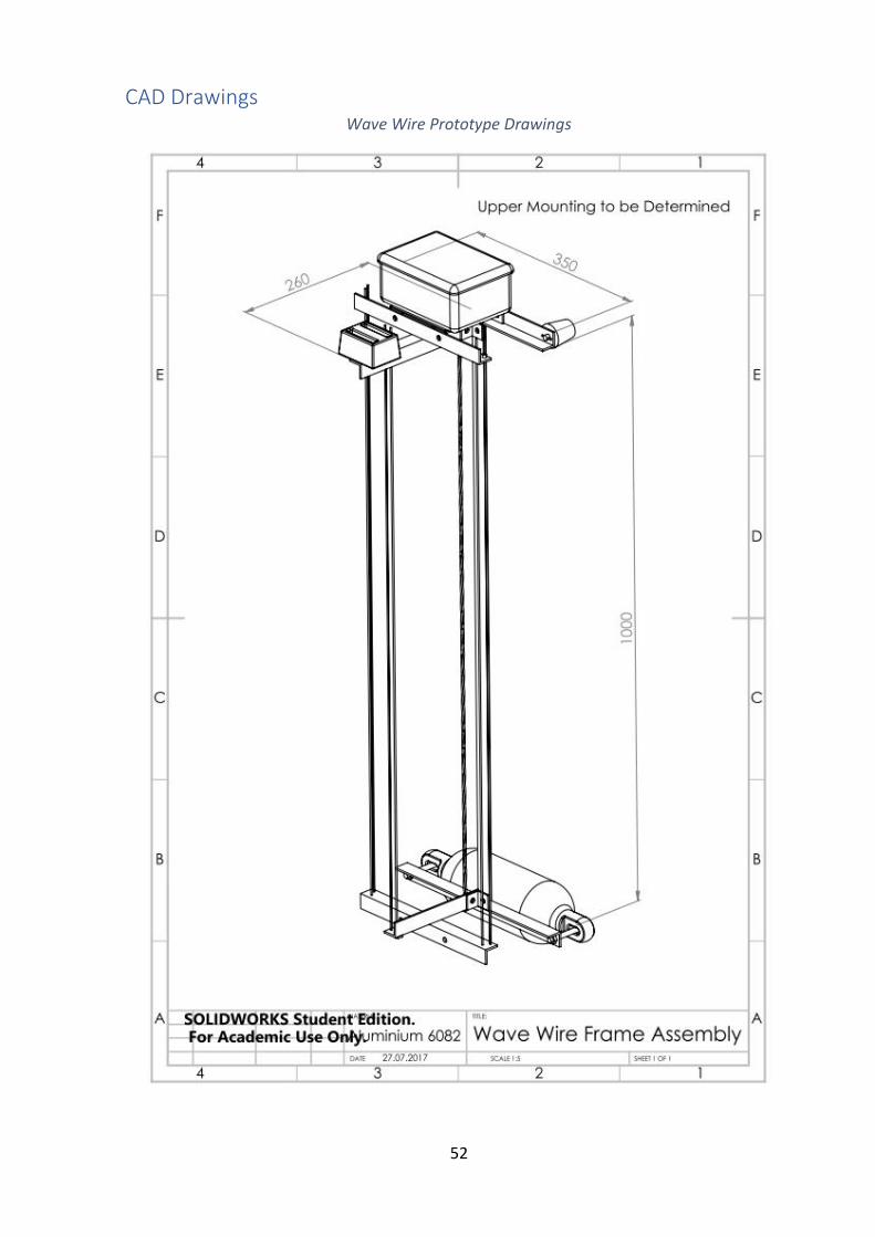
52
CAD Drawings Wave Wire Prototype Drawings
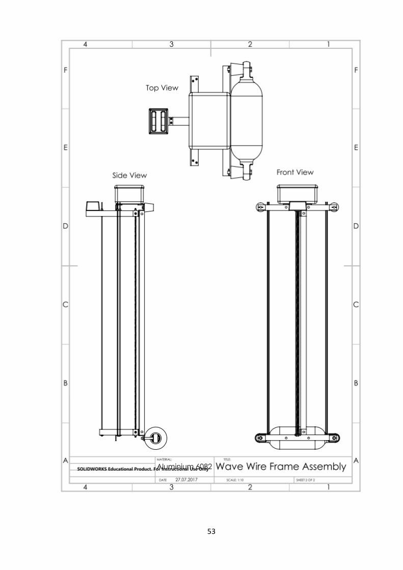
53
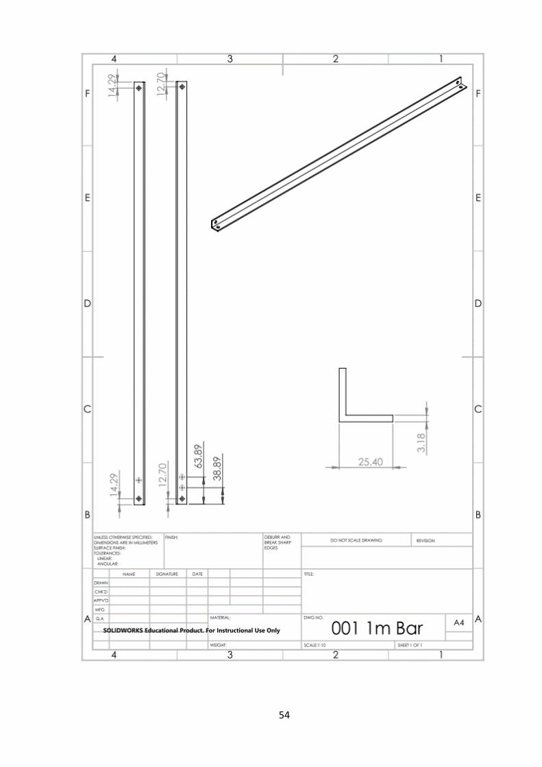
54

55
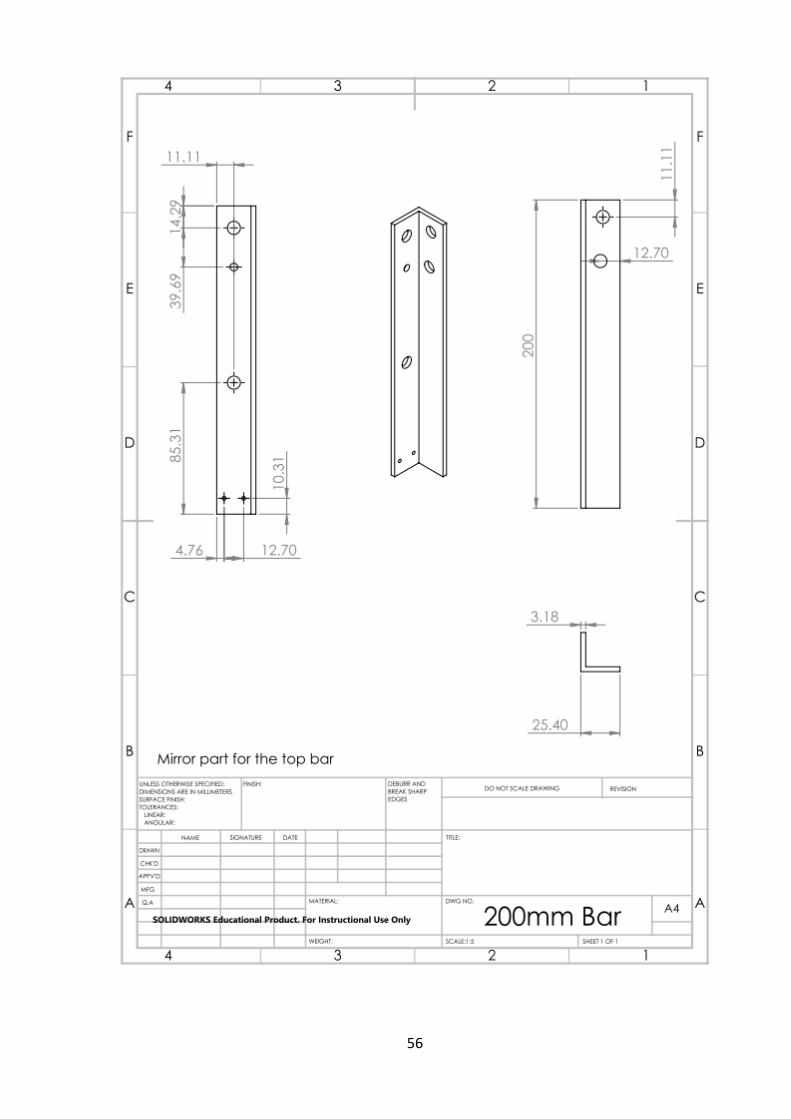
56

57
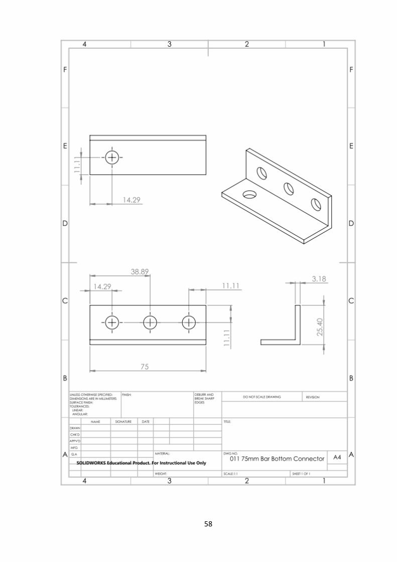
58

59

60
Front Isometric View Back Isometric View

61
Top Isometric View

62
Prototype Photos Overview Photo Top Prototype View
Wire Tightening System Water Tight Container and Wire Connections

63
New Frame Design and Bill of Materials (Via Maytec Software)

64
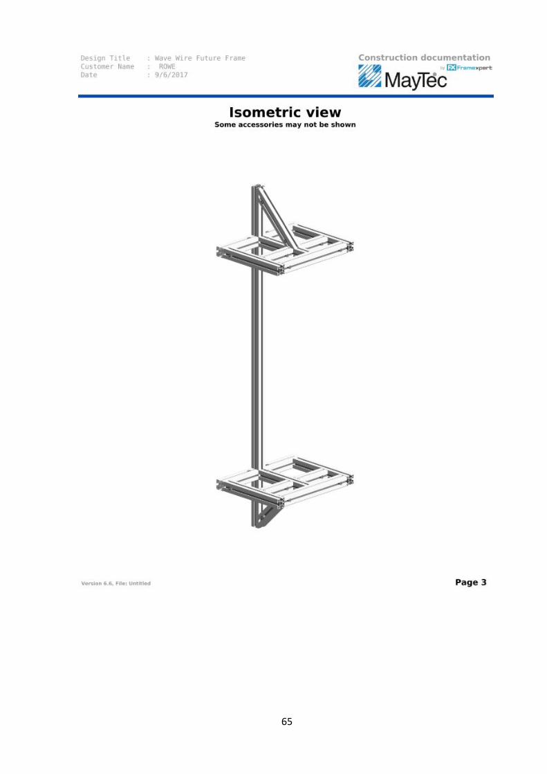
65

66

67
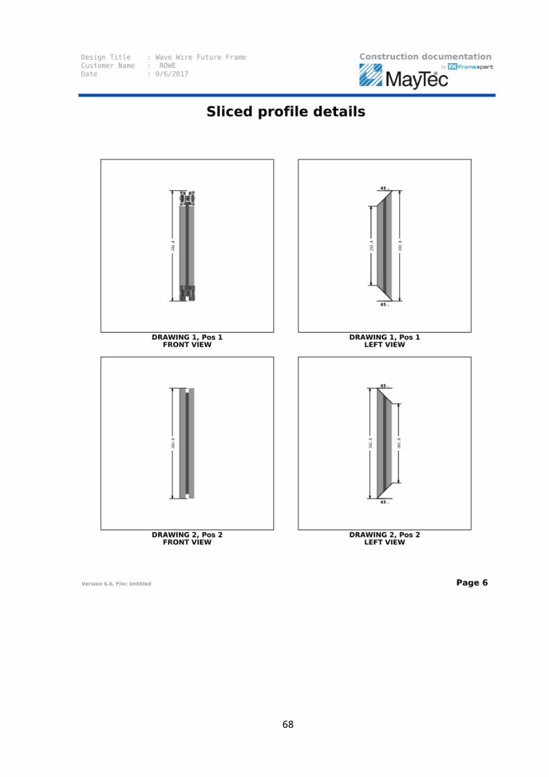
68

69

70
Arduino Code
#include <Wire.h>
#include <Adafruit_MMA8451.h>
#include <Adafruit_Sensor.h>
#include <SD.h>
#include <SPI.h>
unsigned long time;
File myFile;
Adafruit_MMA8451 mma = Adafruit_MMA8451();
#define ADDRESS 0x28
int s = 0;
int x = 0;
float y = 0.0000;
int pinCS = 53; // Pin 10 on Arduino Uno
void setup() {
Serial.begin(9600);
pinMode(pinCS, OUTPUT);
if (SD.begin()) // SD Card Initialization
{
Serial.println("SD card is ready to use.");
} else
{
Serial.println("SD card initialization failed");
return;
}
//----------------------
delay(1000);
Wire.begin();
Wire.beginTransmission(ADDRESS); //Partial
Reset
Wire.write(0x8A);
Wire.endTransmission();
//-----------------------
delay(1000);
Wire.beginTransmission(ADDRESS); //Start CDC
Wire.write(0x8C);
Wire.endTransmission();
//-----------------------
delay(1000);
Wire.beginTransmission(ADDRESS); //Status
Read
Wire.write(0x40);
Wire.write(0x24);
Wire.endTransmission();
Wire.requestFrom(ADDRESS, 1);
while(Wire.available() == 0);
int s = Wire.read();
Serial.print("Status");
Serial.println(s);
Serial.begin(9600);
Serial.println("Adafruit MMA8451 test!");
if (! mma.begin()) {
Serial.println("Couldnt start");
while (1);
}
Serial.println("MMA8451 found!");
mma.setRange(MMA8451_RANGE_2_G);
Serial.print("Range = "); Serial.print(2 <<
mma.getRange());
Serial.println("G");
Serial.print("Time: "); Serial.print("\t");
Serial.print("C1/C0"); Serial.print("\t");
Serial.print("C2/C0"); Serial.print("\t");
Serial.print("C3/C0"); Serial.print("\t");
Serial.println("C4/C0");
myFile = SD.open("wavewire.txt", FILE_WRITE);
if (myFile) {
myFile.println("Start");
myFile.print("Time mils"); myFile.print("\t");

71
myFile.print("C1/C0"); myFile.print("\t");
myFile.print("C2/C0"); myFile.print("\t");
myFile.print("C3/C0"); myFile.print("\t");
myFile.print("C4/C0"); myFile.print("\t");
myFile.println("Z accel");
myFile.close(); // close the file
}
// if the file didn't open, print an error:
else {
Serial.println("error opening test.txt");
}
}
void loop() {
//-----Read C1/C0
time = millis(); //prints time since program
started
Serial.print(time); Serial.print("\t");
Wire.beginTransmission(ADDRESS);
Wire.write(0x40);
Wire.write(0x05);
Wire.endTransmission();
Wire.requestFrom(ADDRESS, 1);
while(Wire.available() == 0);
int c1_3 = Wire.read();
//Serial.print(c1_3); Serial.print(" ");
//---
Wire.beginTransmission(ADDRESS);
Wire.write(0x40);
Wire.write(0x04);
Wire.endTransmission();
Wire.requestFrom(ADDRESS, 1);
while(Wire.available() == 0);
int c1_2 = Wire.read();
//Serial.print(c1_2); Serial.print(" ");
//---
Wire.beginTransmission(ADDRESS);
Wire.write(0x40);
Wire.write(0x03);
Wire.endTransmission();
Wire.requestFrom(ADDRESS, 1);
while(Wire.available() == 0);
int c1_1 = Wire.read();
//Serial.print(c1_1); Serial.print("\t");
float c1_3_f = c1_3;
float c1_2_f = c1_2;
float c1_1_f = c1_1;
float C1 = (c1_3_f * 65536 + c1_2_f * 256 +
c1_1_f)/2097152;
//Serial.print("C1/C0 ");
Serial.print(C1,6); Serial.print("\t");
//-----Read C2/C0
Wire.beginTransmission(ADDRESS);
Wire.write(0x40);
Wire.write(0x08);
Wire.endTransmission();
Wire.requestFrom(ADDRESS, 1);
while(Wire.available() == 0);
int c2_3 = Wire.read();
//Serial.print("C2/C0 "); Serial.print(c2_3);
Serial.print(" ");
//---
Wire.beginTransmission(ADDRESS);
Wire.write(0x40);
Wire.write(0x07);
Wire.endTransmission();
Wire.requestFrom(ADDRESS, 1);
while(Wire.available() == 0);
int c2_2 = Wire.read();
//Serial.print(c2_2); Serial.print(" ");
//---
Wire.beginTransmission(ADDRESS);

72
Wire.write(0x40);
Wire.write(0x06);
Wire.endTransmission();
Wire.requestFrom(ADDRESS, 1);
while(Wire.available() == 0);
int c2_1 = Wire.read();
//Serial.print(c2_1); Serial.print("\t");
float c2_3_f = c2_3;
float c2_2_f = c2_2;
float c2_1_f = c2_1;
float C2 = (c2_3_f * 65536 + c2_2_f * 256 +
c2_1_f)/2097152;
//Serial.print("C2/C0 ");
Serial.print(C2,6); Serial.print("\t");
//-----Read C3/C0
Wire.beginTransmission(ADDRESS);
Wire.write(0x40);
Wire.write(0x0B);
Wire.endTransmission();
Wire.requestFrom(ADDRESS, 1);
while(Wire.available() == 0);
int c3_3 = Wire.read();
// Serial.print("C3/C0 "); Serial.print(c3_3);
Serial.print(" ");
//---
Wire.beginTransmission(ADDRESS);
Wire.write(0x40);
Wire.write(0x0A);
Wire.endTransmission();
Wire.requestFrom(ADDRESS, 1);
while(Wire.available() == 0);
int c3_2 = Wire.read();
//Serial.print(c3_2); Serial.print(" ");
//---
Wire.beginTransmission(ADDRESS);
Wire.write(0x40);
Wire.write(0x09);
Wire.endTransmission();
Wire.requestFrom(ADDRESS, 1);
while(Wire.available() == 0);
int c3_1 = Wire.read();
// Serial.print(c3_1); Serial.print("\t");
float c3_3_f = c3_3;
float c3_2_f = c3_2;
float c3_1_f = c3_1;
float C3 = (c3_3_f * 65536 + c3_2_f * 256 +
c3_1_f)/2097152;
//Serial.print("C3/C0 ");
Serial.print(C3,6); Serial.print("\t");
//-----Read C4/C0
Wire.beginTransmission(ADDRESS);
Wire.write(0x40);
Wire.write(0x0E);
Wire.endTransmission();
Wire.requestFrom(ADDRESS, 1);
while(Wire.available() == 0);
int c4_3 = Wire.read();
//Serial.print("C4/C0 "); Serial.print(c4_3);
Serial.print(" ");
//---
Wire.beginTransmission(ADDRESS);
Wire.write(0x40);
Wire.write(0x0D);
Wire.endTransmission();
Wire.requestFrom(ADDRESS, 1);
while(Wire.available() == 0);
int c4_2 = Wire.read();
//Serial.print(c4_2); Serial.print(" ");
//---

73
Wire.beginTransmission(ADDRESS);
Wire.write(0x40);
Wire.write(0x0C);
Wire.endTransmission();
Wire.requestFrom(ADDRESS, 1);
while(Wire.available() == 0);
int c4_1 = Wire.read();
//Serial.print(c4_1); Serial.print("\t");
float c4_3_f = c4_3;
float c4_2_f = c4_2;
float c4_1_f = c4_1;
float C4 = (c4_3_f * 65536 + c4_2_f * 256 +
c4_1_f)/2097152;
//Serial.print("C4/C0 ");
Serial.print(C4,6); Serial.print("\t");
//------------------------------------------
// Read the 'raw' data in 14-bit counts
mma.read();
//Serial.print("X:\t"); Serial.print(mma.x);
//Serial.print("\tY:\t"); Serial.print(mma.y);
Serial.print("\tZ:\t"); Serial.print(mma.z);
//Serial.print();
Serial.print("\t");
/* Get a new sensor event */
sensors_event_t event;
mma.getEvent(&event);
/* Display the results (acceleration is measured in
m/s^2) */
//Serial.print("X: \t");
Serial.print(event.acceleration.x); Serial.print("\t");
//Serial.print("Y: \t");
Serial.print(event.acceleration.y); Serial.print("\t");
Serial.print("Z: \t");
Serial.print(event.acceleration.z); Serial.print("\t");
Serial.println("m/s^2 ");
/* Get the orientation of the sensor */
uint8_t o = mma.getOrientation();
//-------------------------------------------
myFile = SD.open("wavewire.txt", FILE_WRITE);
if (myFile) {
myFile.print(time); myFile.print("\t");
myFile.print(C1,6); myFile.print("\t");
myFile.print(C2,6); myFile.print("\t");
myFile.print(C3,6); myFile.print("\t");
myFile.print(C4,6); myFile.print("\t");
myFile.println(event.acceleration.z);
myFile.close(); // close the file
}
// if the file didn't open, print an error:
else {
Serial.println("error opening test.txt");
}
}
References
Accelerometer code portion developed alongside -
http://arduinolearning.com/code/arduino-mma8451-accelerometer.php
SD Card code portion developed alongside -
http://howtomechatronics.com/tutorials/arduino/arduino-sd-card-data-logging-excel-
tutorial/

74
Test Setup Photos
Small Scale Prototype Tests Setup (including initial functional tests, salinity variation tests, and temperature variation tests)
Large Scale Prototype Tests (including Static and Dynamic tests in the wave generation tank)

75
River Tests Setup

76
Dynamic Wave Test Additional Results (0.6 Hz and 1.6 Hz Results) 0.6 Hz Wave Test Curves
Dynamic functional test results of full-scale prototype. 0.6Hz, 4cm Amplitude Generation. (a) Complete run - 60 seconds, 42 seconds of waves. (b) Relative zero shift – 15 to 60 second period. (c) Stabilised waves –28 to 38 second period. (d) Stabilised waves, wire 2 only – 28 to 38 second period.

77
1.6 Hz Wave Test Curves
Dynamic functional test results of full-scale prototype. 1.6Hz, 4cm Amplitude Generation. (a) Complete run - 60 seconds, 32 seconds of waves. (b) Relative zero shift – 25 to 60 second period. (c) Stabilised waves – 41 to 51 second period. (d) Stabilised waves, wire 2 only – 41 to 51 second period.

78
Accelerometer Data
This data displays that between time 0 and 150 seconds, upward acceleration averaged higher than the downward acceleration. Between 150 and 325 seconds, negative acceleration averaged higher. After the 325 second mark, the positive acceleration average higher steadily drifting the displacement readings to about 20,000cm. This plot shows the complication of using accelerometers to track actual displacement and the fluctuations that can occur. Other test data shows similar or worse results, i.e. exponential drift instead of steady drift. The calculations used to find displacement from accelerations are equivalent to an integration, where the change in velocity from each previous acceleration data point was calculated with the sample rate time period. The displacement was also calculated this way with the previous velocity data point and the sample rate time period. The equations for these calculations are:
𝑣1 = 𝑣0 + 𝑎0𝑡
𝑦1 = 𝑦0 + 𝑣0𝑡
Where:
v1, is the instantaneous velocity
v0, is the initial velocity or previous data point velocity
a0, is the initial acceleration or previous data point acceleration
y1, is the instantaneous position
y0, is the initial position or previous data point position

79
River Thames Temperature and Salinity Measurement Data
Oyster Pier (West London), Tide In, 1.6.2017, 19:00-21:30
Oyster Pier (West London), Tide Out, 15.6.2017, 19:00-21:30
Blackfriars Bridge, Tide In, 19.7.2017, 8:45-10:45
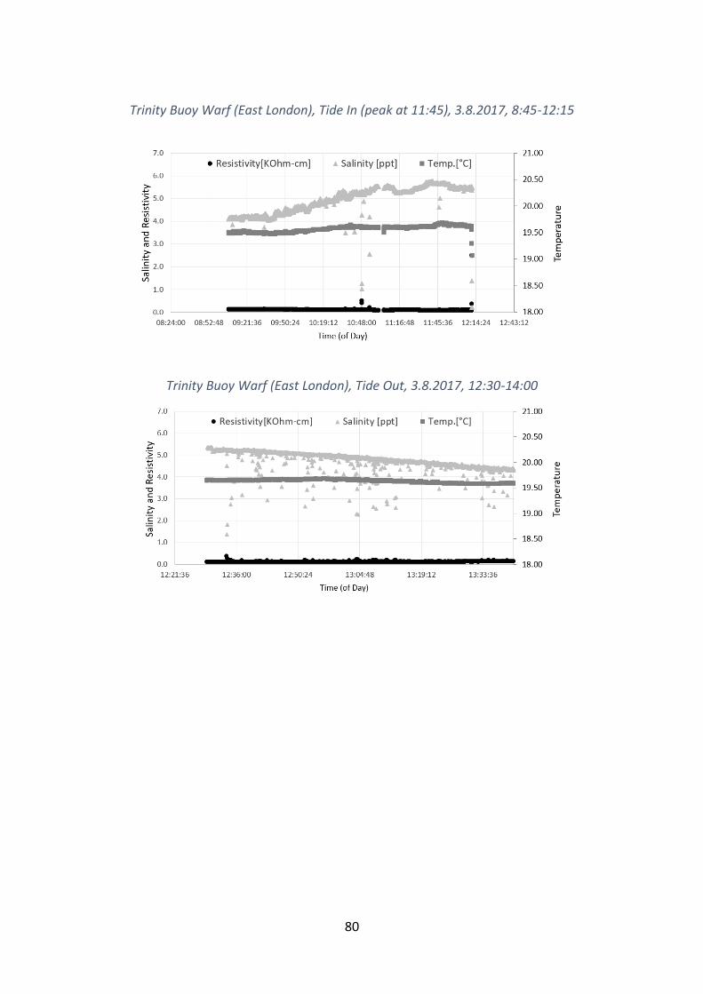
80
Trinity Buoy Warf (East London), Tide In (peak at 11:45), 3.8.2017, 8:45-12:15
Trinity Buoy Warf (East London), Tide Out, 3.8.2017, 12:30-14:00