Waterbed leakage drives EU ETS emissions: COVID-19, the Green Deal & the recovery planKenneth Bruninx 

KU LeuvenMarten Ovaere  ( marten.ovaere@ugent.be )

Ghent University https://orcid.org/0000-0002-8919-3325

Article

Keywords: European Emission Trading System, Waterbed leakage, Carbon Emis- sions, COVID-19,European Green Deal, European recovery plan

Posted Date: March 17th, 2021

DOI: https://doi.org/10.21203/rs.3.rs-270917/v1

License: This work is licensed under a Creative Commons Attribution 4.0 International License.  Read Full License

Version of Record: A version of this preprint was published at Nature Communications on March 4th,2022. See the published version at https://doi.org/10.1038/s41467-022-28398-2.

Waterbed leakage drives EU ETS emissions: COVID-19,

the Green Deal & the recovery plan

Kenneth Bruninx1,2 and Marten Ovaere3,4

1Department of Mechanical Engineering, Faculty of Engineering Science, KULeuven, Belgium

2EnergyVille, Belgium3Department of Economics, Faculty of Economics and Business

Administration, Ghent University, Belgium4School of the Environment, Yale University, USA

February 23, 2021

Because of the EU ETS’ cancellation policy, its fixed cap or waterbed is punctured, meaningthat shocks and overlapping policies can change cumulative carbon emissions, i.e., waterbedleakage. This paper explains the mechanisms behind waterbed leakage and quantifies the effectof COVID-19, the European Green Deal and the recovery stimulus package on cumulative EUETS emissions and allowance prices. We find that the negative demand shock of the pandemichas limited effect on the EU ETS price and is almost completely translated into lower carbonemissions, because of high waterbed leakage. Increasing the 2030 reduction target to -55%increases the price of allowances to 67 e/ton CO2 today and decreases carbon emissions in theperiod 2020-2050 by around 16.3 GtCO2 or 42% of the cumulative cap under current policies.These results are robust to significant changes in allowance demand triggered by overlappingpolicies in the period 2021-2031.

Keywords: European Emission Trading System, Waterbed leakage, Carbon Emis-

sions, COVID-19, European Green Deal, European recovery plan

We are grateful for very helpful comments from Grischa Perino, Arthur Van Benthem, Knut EinarRosendahl, Kenneth Gillingham, Reyer Gerlagh, Erik Delarue, Pieter Vingerhoets, Bram Claeys & RubenBaetens.

1

1 Introduction

The European Union Emissions Trading System (EU ETS), a cornerstone of EU climate policy,is being put to the test by three large shocks affecting carbon emissions: a temporary negativeallowance demand shock because of COVID-19, a positive or negative allowance demand shockbecause of overlapping policies from the NextGenerationEU reovery stimulus package, and apermanent negative allowance supply shock because of the increased emission reduction targetas part of the European Green Deal.

Under an emissions trading system with a fixed cap, these shocks would only affect the priceof carbon emissions, like in the EU ETS during the 2009 recession (Koch et al., 2014), butcumulative emissions would equal the cumulative emissions cap – the so-called waterbed ef-fect.1 However, because the EU ETS’ cancellation policy is conditional on the total numberof allowances in circulation (TNAC) (European Union, 2018), exogenous shocks impacting theTNAC – such as COVID-19, the recovery package or the Green Deal – will affect both carbonprices and cumulative carbon emissions, hence, causing waterbed leakage. Waterbed leakage isdefined as the net effect of a shock or policy on cumulative emissions in EU ETS. It is positivewhen a policy that increases (decreases) emissions in a particular year leads to increased (de-creased) cumulative emissions, and negative when a policy backfires. For example, waterbedleakage is 0.5 if a shock decreases emissions by 4 MtCO2 and cumulative emissions by 2 MtCO2.

First, we discuss the three factors that affect waterbed leakage and provide a graphical summaryof its magnitude, depending on the year of the shock and the year in which the waterbed issealed again. Second, we quantify the individual and joint effect of the COVID-19, EuropeanGreen deal and stimulus package shocks on allowance prices and total cumulative emissions.Because of the large uncertainty in this forward simulation, we present a range of results thatcrucially depend on when the waterbed will be sealed again.

2 The punctured waterbed of the EU ETS

The European Union Emissions Trading Scheme (EU ETS) limits emissions from the electricpower sector, the energy-intensive industry and intra-European aviation. This cap-and-tradesystem covers around 45% of the EU’s greenhouse gas emissions, equaling 1562 MtCO2 in 2019(European Commission, 2020a, 2019).

To address the large surplus of allowances in the system and to structurally signal future scarcityof emission allowances, the EU strengthened the EU ETS by adding a cancellation policy toits market stability reserve (MSR) (European Union, 2018). If the number of allowances incirculation (TNAC) surpasses 833 MtCO2, the MSR absorbs a share of the allowances to beauctioned, so that they can be released again from the reserve in the future when allowances arescarce. Starting in 2023, however, a cancellation policy will be in effect, such that allowancesheld in the MSR exceeding the amount auctioned during the previous year will be canceled(European Union, 2018).

Without the cancellation policy, individual actions to reduce emissions only affect who emitsand at what price, but not what ultimately matters, which is how much is emitted in totalunder the fixed cap – the waterbed effect (Perino, 2018). However, with a cancellation policy

1This effect is described using the analogy of a waterbed because you can push down on a waterbed in anylocation, but the total volume of water in the bed remains the same (Perino, 2018).

2

in effect, changes to allowance demand, such as overlapping policies (Bertram et al., 2015;Perino, 2018; Perino et al., 2020; Rosendahl, 2019b; Bruninx et al., 2019), strategies to buy,bank, and burn allowances (Gerlagh and Heijmans, 2019), or exogenous shocks may resultin changes to cumulative emissions – waterbed leakage. Waterbed leakage depends on threefactors: the direct effect of cancellation (Appendix A.1), the indirect effect of expectationsthrough adjustments of the price profile (Appendix A.2), and the (change in) duration of thewaterbed puncture (Appendix A.3).

3 Waterbed leakage: impact on cumulative emissions

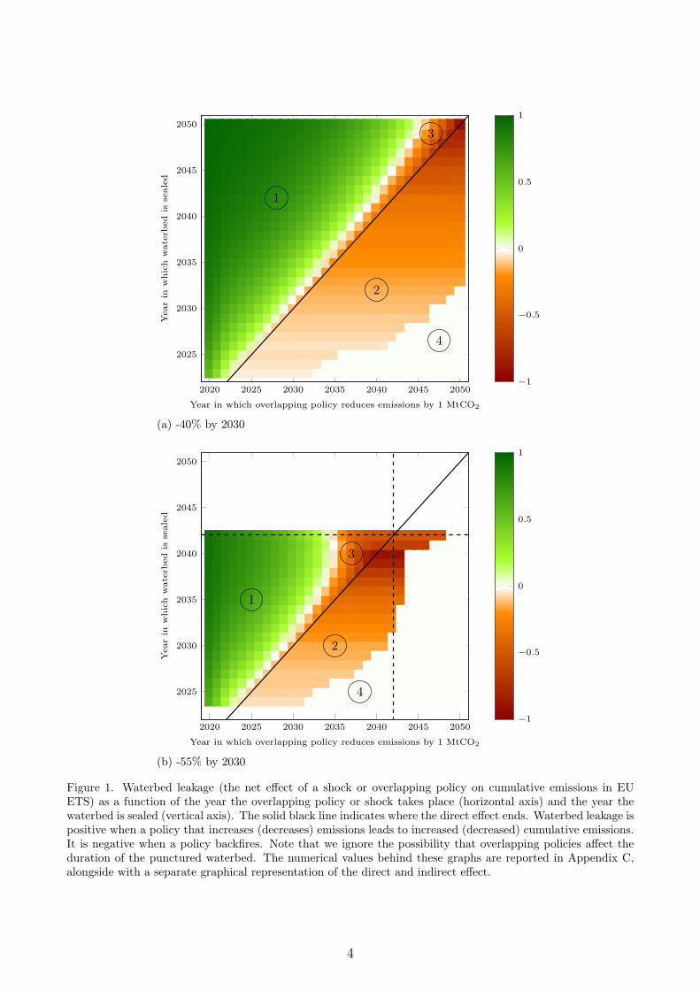
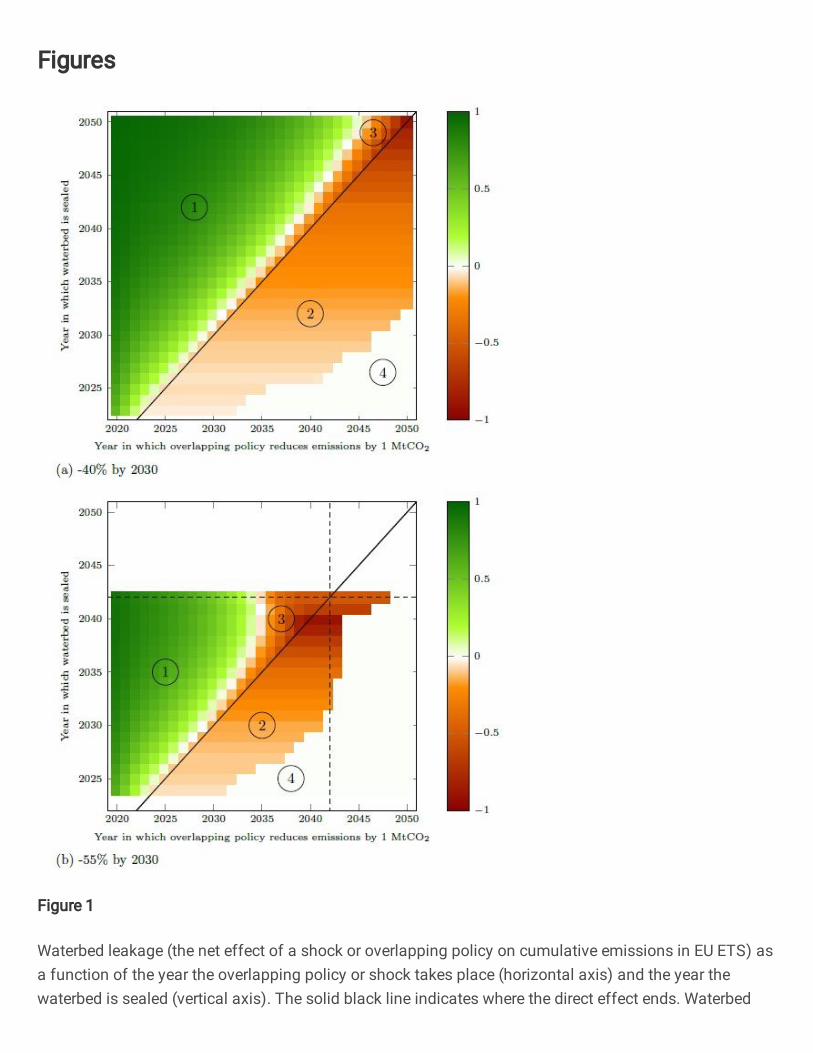
Because of the punctured waterbed, the effect of overlapping policies on cumulative emissions– waterbed leakage – is not obvious and depends on the year the policies are announced, thetime profile of their effect on emissions, and the year in which the waterbed is sealed (Beck andKruse, 2020; Bruninx et al., 2019; Gerlagh and Heijmans, 2019; Gerlagh et al., 2020b; Perinoet al., 2020; Rosendahl, 2019a). Figure 1 presents a graphical summary of waterbed leakagedepending on two of the above three dimensions: the year in which the overlapping policyreduces emissions on the horizontal axis and the year in which the waterbed is sealed on thevertical axis – assuming that the policy is announced in 2020. For details on the mathematicalmodel used to derive these results, we refer the reader to Appendix B. Importantly, we ignorethe possibility that overlapping policies affect the duration of the punctured waterbed, seeSection A.3, which could lead to waterbed leakage that can have any positive or negative value.Hence, in this section, waterbed leakage is always between -1 and 1.

We can identify four different regions in Figure 1, based on the relative importance of thedirect effect of the policy on emissions (Perino, 2018) and the indirect price effect caused bythe adjustment of the equilibrium price (Rosendahl, 2019b; Bruninx et al., 2019).2 First, inthe upper-left part of the figure, the direct effect dominates, because the overlapping policyis executed well before the waterbed is sealed. In that case, changes to the TNAC affectcancellation over an extended period, as explained by Perino (2018). In the most extreme case,i.e., executing an overlapping policy in 2020 and the waterbed sealing in 2050, direct waterbedleakage nearly equals one. In other words, abatement now decreases cumulative emissions bythe same amount. On the other hand, the closer the effect of the overlapping policy is to theyear in which the waterbed is sealed, the lower the direct effect.

Second, below the diagonal line, the direct effect is zero as the overlapping policy only reducesemissions after the waterbed is sealed again. However, waterbed leakage is not zero, because ofthe indirect effect of announced future overlapping policies on the equilibrium price path, whichaffects emissions before the waterbed is sealed. This indirect price effect is negative, meaningthat overlapping policies backfire: abatement efforts lead to an increase in cumulative emissions,announced increases in emissions lead to a decrease in cumulative emissions. This ‘new greenparadox’ was first described by Rosendahl (2019a). Importantly, for a given duration of thewaterbed puncture, the indirect effect increases with the time between the announcement of apolicy and when it takes place (Gerlagh et al., 2020b). But as soon as the waterbed is sealed,the indirect effect becomes independent of the year in which the policy is executed (Gerlaghet al., 2020b).

2Figure 3 in Appendix C presents the direct and indirect separately.

3

2020 2025 2030 2035 2040 2045 2050

2025

2030

2035

2040

2045

2050

Year in which overlapping policy reduces emissions by 1 MtCO2

Yearin

which

waterb

ed

issealed

−1

−0.5

0

0.5

1

1

3

2

4

(a) -40% by 2030

2020 2025 2030 2035 2040 2045 2050

2025

2030

2035

2040

2045

2050

Year in which overlapping policy reduces emissions by 1 MtCO2

Yearin

which

waterb

ed

issealed

−1

−0.5

0

0.5

1

1

3

2

4

(b) -55% by 2030

Figure 1. Waterbed leakage (the net effect of a shock or overlapping policy on cumulative emissions in EUETS) as a function of the year the overlapping policy or shock takes place (horizontal axis) and the year thewaterbed is sealed (vertical axis). The solid black line indicates where the direct effect ends. Waterbed leakage ispositive when a policy that increases (decreases) emissions leads to increased (decreased) cumulative emissions.It is negative when a policy backfires. Note that we ignore the possibility that overlapping policies affect theduration of the punctured waterbed. The numerical values behind these graphs are reported in Appendix C,alongside with a separate graphical representation of the direct and indirect effect.

4

Third, the indirect price effect is larger when the waterbed is sealed later and the policy isannounced today, but executed later. As a result, waterbed leakage tends to -1 in the upper-right corner of Figure 1. Note furthermore that the indirect effect may dominate the directeffect in the years preceding the year in which the waterbed is sealed, yielding negative waterbedleakage in regions where one intuitively expects positive values.

Fourth, as soon as there are no more banked allowances and the total number of allowancesin circulation is zero, there is no more inter-temporal arbitrage and waterbed leakage is zero.Both the direct effect and the indirect price effect will be zero and the EU ETS once again putsa strict cap on emissions. Overlapping policies will not have any effect on cumulative emissions,but will affect the EU ETS price.

4 The impact of COVID-19, the Green Deal and the

recovery plan

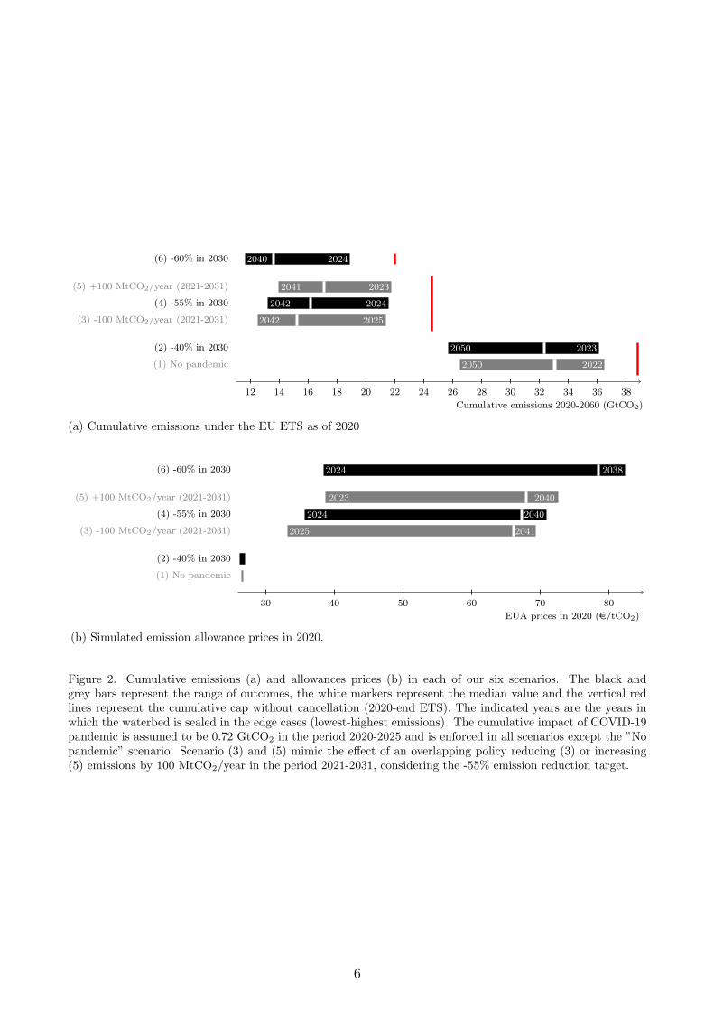
Figure 2 summarizes the simulated (a) cumulative emissions and (b) allowances prices for eachof six scenarios, which are constructed as follows.3 Scenario (1) and (2) consider the current-40% carbon reduction target by 2030, whereas scenarios (3)–(5) and (6) consider a reductiontarget of -55% and -60%, reflecting the implementation of the Green Deal.4 Scenario (1) doesnot consider the impact of COVID-19 (-0.72 GtCO2 in the period 2020-2025), whereas all otherscenarios do. Scenario (3) and (5) mimic the effect of an overlapping policy – induced by therecovery stimulus package – affecting emission allowance demand by 100 MtCO2/year in theperiod 2021-2031, considering the -55% emission reduction target.

The vertical red lines represent the cumulative cap (2020-end ETS), including the surplus atthe end of 2019 European Commission (2020b), in the absence of any cancellation. This meansa cumulative cap of 38.8 GtCO2 under the current policy scenario of a 40% carbon reductiontarget in 2030 (‘-40% in 2030’). Because the pandemic does not affect the cumulative cap,it is equal under the second scenario (‘-40% in 2030’). When the carbon reduction target in2030 is increased to -55% (‘-55% in 2030 pandemic’) and -60% (‘-60% in 2030 pandemic’), thecumulative cap lowers to 24.6 GtCO2 and 22.0 GtCO2.

The black and gray bars represent simulated cumulative emissions in each of the six scenarios.Because of cancellation, cumulative emissions are always lower than the cumulative emissionscap. In the pre-pandemic scenario (1), median expected cumulative emissions are 33.2 GtCO2,which is 5.6 GtCO2 lower than the fixed cap. However, there is a large range of uncertaintyaround these results, depending on when the waterbed is sealed again (indicated by the datesin the bars), which depends on a number of factors (see Appendix A.3). For example, totalcancellations are only 2.7 GtCO2 when the waterbed is already sealed in 2022. On the otherhand, when the waterbed only seals in 2050, more allowances are cancelled and cumulativeemissions in the pre-pandemic scenario are only 26.7 GtCO2.

3Detailed descriptions of the scenarios can be found in Appendix B.4For ease of referencing, we characterize our scenarios based on the overall European emission reduction target

(-40%, -55% or -60%) relative to 1990 emission levels. Recall, however, that the emission reduction targets forthe sectors covered by EU ETS are more stringent: -43%, -57.75% (estimated) and -63% (estimated), relativeto 2005 emission levels.

5

12 14 16 18 20 22 24 26 28 30 32 34 36 38

(1) No pandemic

(2) -40% in 2030

(3) -100 MtCO2/year (2021-2031)

(4) -55% in 2030

(5) +100 MtCO2/year (2021-2031)

(6) -60% in 2030

20222050

20232050

20252042

20242042

20232041

20242040

Cumulative emissions 2020-2060 (GtCO2)

(a) Cumulative emissions under the EU ETS as of 2020

30 40 50 60 70 80

(1) No pandemic

(2) -40% in 2030

(3) -100 MtCO2/year (2021-2031)

(4) -55% in 2030

(5) +100 MtCO2/year (2021-2031)

(6) -60% in 2030

2025 2041

2024 2040

2023 2040

2024 2038

EUA prices in 2020 (e/tCO2)

(b) Simulated emission allowance prices in 2020.

Figure 2. Cumulative emissions (a) and allowances prices (b) in each of our six scenarios. The black andgrey bars represent the range of outcomes, the white markers represent the median value and the vertical redlines represent the cumulative cap without cancellation (2020-end ETS). The indicated years are the years inwhich the waterbed is sealed in the edge cases (lowest-highest emissions). The cumulative impact of COVID-19pandemic is assumed to be 0.72 GtCO2 in the period 2020-2025 and is enforced in all scenarios except the ”Nopandemic” scenario. Scenario (3) and (5) mimic the effect of an overlapping policy reducing (3) or increasing(5) emissions by 100 MtCO2/year in the period 2021-2031, considering the -55% emission reduction target.

6

Adding the COVID-induced negative demand shock of 0.72 GtCO2 in the period 2020-2025(scenario (2)), we find that it is largely translated into lower cumulative emissions. As discussedin Section A.1, the longer the duration of the waterbed puncture, the larger the share of theadditional 0.72 GtCO2 allowances that is cancelled. Importantly, because the negative demandshock induced by COVID measures increases the number of allowances in circulation, it willprolong the waterbed puncture. For example, in cases where the total number of allowancesin circulation is low and the waterbed was expected to be closed in 2022, the negative demandshock of COVID extends the puncture to 2023.

Raising the ambition for 2030 to -55% or -60% (scenarios (4) and (6)), Figure 2 shows that theduration of the waterbed puncture increases to 2024 in the cases with the highest cumulativeemissions. In line with our discussion in Section A.3, we find that median expected cumulativecancellations increase with approximately 2 GtCO2 – from 5.6 GtCO2 to 7.6 GtCO2. Note thatthis counter-intuitive self-reinforcing effect, first discussed in (Bruninx et al., 2020, 2019), isless pronounced for the cases with lowest cumulative emissions, as these cases are characterizedby shorter waterbed punctures.5

Finally, in scenarios (3) and (5) we add a shock to scenario (4) of -100 or +100 MtCO2/year overthe 2021-2031 period. This is an illustration of the effect of an overlapping policy, like renewablesupport (scenario (3)) or electric vehicles (scenario (5)). In line with the values in Figure 1, wefind that the effect of these policies is almost completely translated into lower (3) or higher (5)cumulative emissions if the waterbed is punctured for a long time – indicating waterbed leakageclose to one – as the direct effect dominates (scenario (3) and (5)) and the waterbed is sealedsooner (scenario (5)). When the waterbed is sealed soon, the effect on cumulative emissions is,as expected, lower. In these cases, the overlapping policy extends beyond the year in which thewaterbed is sealed, such that the indirect effect dominates the direct effect in later years.

Zooming in on Figure 2(b), we find that the negative demand shock of the pandemic (scenario(2)) has a limited effect on the price of allowances in 2020. The raised ambitions, however,increase the price to a median value of 67 e/ton CO2 (-55%) to 79 e/ton CO2 (-60%) in2020. Although EU ETS prices are currently at all-time highs, just below 40 e/tCO2, which iswithin the estimated range in Figure 2(b), they are still at levels well below our median values,indicating that, for various reasons, the stringency of the new 2030 targets may have not yetbeen fully internalized by the market. The estimated EUA price is lower when the waterbed issealed sooner and cancellation is lower. The price changes because of the overlapping policies inscenario (3) and (5) are higher when the waterbed is sealed sooner, because a smaller fractionof the shock is absorbed through cancellation.

5This counter-intuitive, self-reinforcing effect may be explained via the relation between the future costof abatement and the cancellation volume. Cancellation volumes increase when the expected future cost ofabatement is higher, as it makes banking allowances today more profitable, which increases the TNAC. Thisimplies that the cancellation policy is more stringent when the cost of compliance is higher. Future abatementcosts increase when, e.g., the linear reduction factor increases or when overlapping policies increase emissionsin the future. For details, see Bruninx et al. (2020, 2019).

7

5 Conclusions

We quantify the effect of COVID-19, the European Green Deal and the recovery stimuluspackage on emission allowance prices and cumulative emissions in the EU ETS. Under a fixedcap, the negative allowance demand shock induced by the pandemic would only reduce pricesand keep emissions fixed. Because of the punctured waterbed, we find that the temporarydecrease in emissions almost one-to-one translates into a decrease of cumulative emissions, withlimited effect on the EU ETS price, in line with the observed price recovery in 2020. This makesclear that the increased price stability due to the introduction of the market stability reserveand the cancellation policy has come at the expense of increased uncertainty in cumulativeemissions.

Raising the ambition for 2030 to -55% or -60% will decrease cumulative EU ETS emission byanother 18 or 21 GtCO2. There is, however, a large range of uncertainty around these results,depending on when allowance cancellation stops and the waterbed is sealed again. This cruciallydepends on external shocks (e.g., COVID-19), overlapping policies (e.g., recovery stimuluspackage), European climate policy, and the shape of the abatement cost curve. The magnitudeof waterbed leakage depends on the relative importance of the direct effect of the policy onemissions and the indirect price effect. We find, among other things, that all overlapping policiesannounced now and affecting emissions after the waterbed is expected to be sealed will backfire.For example, announcing today to close a coal-fired power plant in the future, might actuallyincrease cumulative emissions over the lifetime of EU ETS, in absence of proper companionpolicies (e.g., voluntary cancellation of emission allowances (European Union, 2018)).

Most of the surprising and counter-intuitive aspects of the current EU ETS design that we iden-tified in this paper arise because the supply of allowances depends on the scarcity of allowancesin circulation, which makes cumulative emissions endogenous and exacerbates quantity uncer-tainty. In light of the upcoming 2021 review of the EU ETS, Perino et al. (2021) propose thatallowance supply could be conditioned on the price of allowances instead of the total number ofallowances in circulation, similar to the California cap-and-trade system. This has the potentialto stabilize prices, but might not sufficiently decrease the uncertainty on cumulative emissionsand might lead to oscillatory price behavior between the price cap and floor, as analyzed byBorenstein et al. (2019). This may be an interesting question for future research.

Acknowledgement

K. Bruninx is a post-doctoral research fellow of the Research Foundation - Flanders (FWO) atthe University of Leuven and EnergyVille. His work was funded under postdoctoral mandateno. 12J3320N, sponsored by FWO.

8

A Direct effect, indirect effect and duration of the wa-

terbed puncture

A.1 The direct effect

When actions change the TNAC, this will directly translate into changing levels of cancellation.This is not a one-to-one relationship, as the market stability reserve only absorbs a share ofthe TNAC in a given year – 24% from 2019 till 2023 and 12% from 2024 onward (EuropeanUnion, 2018). As a result, changes in allowance supply or demand are gradually transferred tothe market stability reserve and cancelled. For every ton of CO2 affected by the overlappingpolicy, direct cancellation of allowances equals (Perino, 2018):

1− (1− 0.24)n · (1− 0.12)m (1)

where n and m are the number of years between the time of increasing the TNAC and theyear the waterbed is sealed again (i.e., when the TNAC is below the 833 MtCO2 threshold),with intake rates of 24% and 12% (Bruninx et al., 2020). This means that the direct effect ishigher when the action is earlier and the waterbed is sealed later. Actions taking place afterthe waterbed has been sealed again will not have a direct effect.

A.2 The indirect price effect or new green paradox

All actions that are announced before they take place will have an effect on the TNAC, ir-respective of when the waterbed is sealed again, because of an indirect effect of expectationsthrough adjustments of the price profile (Bruninx et al., 2019; Gerlagh et al., 2020b; Perinoet al., 2020; Rosendahl, 2019a). For example, when a future action announced today, like acoal plant closure, is expected to increase the total number of allowances in circulation at somepoint in the future, market participants expect the future price of allowances to drop. BecauseEU ETS allowances have an infinite lifetime, the future drop in allowance prices will lead tolower prices today, assuming market participants are intertemporally optimizing. As a result,the incentive to abate today will decrease because of expected carbon abatement in the future.Similarly, announced future decreases of the TNAC will lead to higher abatement and a higherTNAC today.

Closed-form expressions for the indirect price effect do not exist – it may only be estimatednumerically (Section 3). However, in general, one may state that the indirect price effect (i)works in the opposite direction as the direct effect; (ii) persists as long as the policy affectsemissions in a period that the TNAC is not zero, hence, firms are still intertemporally optimizingor banking; (iii) is strongest when the policy affects emissions after the waterbed is sealed againand (iv) is stronger when the waterbed seals later.

A.3 The duration of the waterbed puncture

From the discussion above, it is evident that the duration of the waterbed puncture cruciallyaffects the relative importance of the direct and indirect effect. The duration of the waterbedpuncture is determined by the moment when the total number of allowances in circulation falls

9

below 833 MtCO2, i.e., when the market stability reserve stops absorbing allowances. As aresult, all changes to the TNAC can potentially affect the duration of the waterbed puncture,if it pushes the TNAC to be above or below the threshold. We discuss three distinct waysthe TNAC, hence, the duration of the waterbed puncture, may change: expectations aboutmarginal abatement costs, overlapping policies and exogenous shocks, and the design of EUETS itself.

First, expectations about future abatement costs will affect the TNAC today. If firms expecthigher abatement costs in the future, i.e., a more convex marginal abatement cost curve, theywould likely choose to abate more today and bank the surplus allowances for future use. Butbecause of the cancellation policy, if more allowances are banked today, the duration of the wa-terbed puncture may increase, more allowances will be cancelled, and the cumulative emissionsreductions would be greater. In contrast, if firms expect future abatement costs to be low, e.g.,because of technological learning (Creutzig et al., 2017), they would likely choose to postponeabatement and bank fewer allowances. With fewer banked allowances, the waterbed could besealed sooner, fewer allowances would be cancelled, and cumulative emissions reductions wouldbe lower (Rosendahl, 2019b). The design of the cancellation policy thus implies a counter-intuitive, self-reinforcing relation between the future cost of abatement and the cancellationvolume, making the cancellation policy more stringent when the cost of compliance is higher –an effect first discussed by Bruninx et al. (2020, 2019).6 Although future marginal abatementcosts are intrinsically uncertain (Borenstein et al., 2019), there is evidence that the marginalabatement cost curve is (highly) convex (Hintermayer et al., 2020; Landis, 2015).

Second, any European, national or local policy that affects the demand for allowances maychange the TNAC and the duration of the waterbed puncture. For example, support for electricvehicles increases the demand, because gasoline (not covered by EU ETS) is substituted byelectricity (covered by EU ETS), while support for renewable generation or the forced closureof a coal plant decreases it. As a result, the first measure may decrease the duration of thewaterbed puncture, while the second may increase it: depending on the amount of emissionsaffected and timing of the policy, the year in which the waterbed is sealed may change.

Third, expected changes to the design of EU ETS, i.e., the supply of allowances, will affect theTNAC today and hence potentially change the duration of the waterbed puncture. For example,increasing the future linear reduction factor may prolong the puncture of the waterbed, becausemore costly future abatement leads to more abatement now. As a result, the linear reductionfactor and cumulative emissions are positively correlated, meaning that decreasing the long-run supply of allowances increases cancellation volumes (Bruninx et al., 2020). Again, thisunderlines the counter-intuitive, self-reinforcing relation between the linear reduction factor –driving the cost of abatement – and the cancellation volume, making the cancellation policymore stringent when the cost of compliance is higher.

Note that the effect of any overlapping policy, shock or EU ETS design change on the durationof the waterbed puncture may be interpreted via its impact on firms’ expectation on the costof complying with the emissions cap.

6This surprising result crucially depends on the assumption that market participants are inter-temporally-optimizing over the full horizon of the EU ETS. Indeed, in models with a limited horizon, like in Quemin andTrotignon (2019), market participants do not consider the challenges further in the future and will abate less,which decreases cumulative cancellation. As a result, the positive correlation between the convexity of themarginal abatement cost curve and cancellation increases the more market participants look further into thefuture, assuming they face the same marginal abatement cost curve.

10

B Methods

B.1 Simulation model

We analyze the impact of these three shock on the emission allowance price and allowed emis-sions under EU ETS, leveraging our stylized EU-ETS-MSR model (Bruninx et al., 2019). Thismodel is based on the detailed long-term investment model of Bruninx et al. (2020) and as-sumes rational, price-taking and risk-neutral firms that optimize their abatement and bankingactions over the complete EU ETS horizon.

Since the marginal abatement cost curve of the EU ETS is fundamentally uncertain, we runeach demand shock scenario for a comprehensive set of marginal abatement cost curves, whichall adhere to the following functional form:

∀t∈T : pt = β · (E − qt)γ (2)

In each year t, the marginal abatement cost pt is defined by baseline emissions E, a slope β

and a curvature γ, following Bruninx et al. (2019).

Baseline emissions are set to 1900 MTCO2, as in Perino and Willner (2017). The real discountrate is set to 8%. The curvature γ is varied between 0.5 and 3.5, with increments of 0.05. Foreach curvature value, the slope of each abatement cost curve is calibrated to reproduce theaverage 2019 emission allowance prices (24.7 e/tCO2, based on EEX (Last accessed: April 1,2020)) without the negative demand shocks and assuming a -40% emission reduction targetby 2030, in line with 2019 policy, while imposing observed emissions in 2019 and the state ofthe EU ETS at the start of 2019 (European Commission, 2020a). Note that the Green Dealwas first announced in December 2019, and hence, is assumed not to be internalized by marketparties in the average 2019 prices. γ-values below 0.5 yield emissions in 2020 that would exceed2017 levels, which is, at current emission allowance prices, deemed unrealistic. γ-values above3.5 lead to waterbed closures after 2050.

This approach allows simulating the impact of waterbed closures in any year between 2022 and2050 (Fig. 2) in absence of a demand shock: as the curvature increases, the waterbed is sealedlater - as will be discussed in Section A.3. Note that we do not aim to quantify which abatementcost curve is more realistic and that all simulated abatement cost curves are consistent with2019 emission allowance prices.

For more information on the numerical model and the solution strategy, see Bruninx et al.(2019) and Bruninx et al. (2020).

B.2 Estimating waterbed leakage

To estimate the direct and indirect effect of an overlapping policy (Figure 1) , we take thefollowing approach. From the set of calibrated marginal abatement cost curves (see above), weselect a subset that ensures that each year in which the waterbed may be sealed (2023-2050)occurs in the output once. For each of these marginal abatement cost curves, we computea reference equilibrium emission and EUA price path assuming a -40% or -50% emission re-duction target for 2030, considering the impact of COVID-19. In a second set of simulations,considering the same marginal abatement cost curves and policy boundary conditions, we add

11

an overlapping policy reducing emissions by 1 MtCO2 in a year between 2020 and 2050. Com-paring cumulative emissions in the second set of simulations to the corresponding referenceresult yields an estimate of the waterbed effect.

Note that the estimates in Figure 1 pertain to policies affecting emissions in a single year. Thetotal waterbed leakage of a policy or a combination of policies spanning over different years canbe calculated as the weighted sum of its effect over time, assuming they do not affect the yearin which the waterbed is sealed:

∑t

∑i WLt(tsealed) · qit∑

t

∑i |qit|

(3)

where qit is the effect (in tons of CO2) of policy i in year t on the total number of allowances incirculation, while WLt(tsealed) is the magnitude waterbed leakage in year t, which is a functionof the year the waterbed is sealed tsealed. To make this more useful for researchers and policymakers, Tables C1 and C2 in Appendix C present the values of the waterbed leakageWLt(tsealed)for t ∈ [2020, 2050] and tsealed ∈ [2023, 2050].

B.3 The three exogenous shocks affecting the EU ETS

To estimate the impact of the three exogenous shocks, we compute an equilibrium emission andprice path for each of the calibrated marginal abatement cost curves in six policy scenarios.The sections below discuss in more detail the assumptions behind the six scenarios consideredin Section 4.

B.3.1 COVID-19: a temporary negative allowance demand shock

The coronavirus pandemic and lockdown measures that combat it have drastically reduced en-ergy demand throughout the world (Gillingham et al., 2020; Le Quere et al., 2020; Liu et al.,2020). The final effect on 2020 carbon emissions of EU ETS firms is still unclear until the nextpublication of the total number of allowances in circulation by May 2021 (European Commis-sion, 2020a). Other papers on EU ETS focusing entirely on COVID-19 (Azarova and Mier,2020; Bruninx and Ovaere, 2020; Gerlagh et al., 2020a) all study three alternative scenariosregarding the severity and duration of the negative demand shock, similar to a U-shaped fastrecovery, a V-shaped gradual recovery, and a profound recession or permanent demand shock.To limit the number of scenarios, in this paper we only simulate a U-shaped demand shock,which gradually vanishes between 2020 and 2025. We assume the demand shock linearly de-creases from its initial value in 2020, 240 MtCO2 (the worst-case estimate in (Bruninx andOvaere, 2020)), to zero at the end of 2025. The total negative demand shock is, hence, 720MtCO2.

B.3.2 Increased carbon abatement targets under the European Green Deal: per-

manent negative allowance supply shock

As part of the European Green Deal aiming to make the EU’s economy sustainable and reachclimate neutrality by 2050, the European Commission plans to reduce EU greenhouse gasemissions by at least 55% by 2030, compared to 1990 levels, up from the earlier target of 40%

12

(European Commission, 2020b). As of today, it is unclear how this target, covering all sectors,will translate into more ambitious targets for sectors covered under the EU ETS and higherlinear reduction factors in the 2021 EU ETS review. In line with the previous 2030 EU ETStarget of -43% relative to 2005 emission levels, we will assume that the future linear reductionfactor will increase to reach a 57.75% carbon reduction target in the EU ETS by 2030, relativeto emission levels in 2005 - which is achieved by increasing the linear reduction factor to 3.77 %.Because the European Parliament voted to update this target to a 60% reduction target relativeto 1990, we will also run a scenario with a -63% target relative to 2005 emission levels for sectorscovered by EU ETS, with a linear reduction factor of 4.33 %. Such increased linear reductionfactors are considered to be a permanent negative allowance supply shock. We assume that allconsidered linear reduction factors are kept constant after 2030 until the supply is zero.

B.3.3 NextGenerationEU recovery stimulus package: a short- to long-term nega-

tive or positive allowance demand shock

To help repair the economic and social damage caused by the coronavirus pandemic, the EUagreed on the e750 billion NextGenerationEU recovery stimulus package, of which 37% will bespent directly on European Green Deal objectives, like hydrogen, building renovations and onemillion electric charging points. In addition, the entire e1.1 trillion EU budget for 2021-2027will also have to follow the ‘Do No Significant Harm’ principle, which prohibits investments infossil fuels and other technologies deemed contrary to the EU’s environmental objectives. Asthe additional overlapping policies funded by this budget can affect the demand for EU ETSallowances at different times and in many different ways, we will only simulate two genericscenarios. One that increases demand for allowances by 100 MtCO2 per year from 2021 to 2031(e.g., electric vehicles), and one that decreases demand for allowances by 100 MtCO2 per yearfrom 2021 to 2031 (e.g., renewables support).

13

C Detailed results

2020 2025 2030 2035 2040 2045 2050

2025

2030

2035

2040

2045

2050

Year in which overlapping policy reduces emissions by 1 MtCO2

Yearin

which

waterb

ed

issealed

−1

−0.5

0

0.5

1

(a) Direct effect

2020 2025 2030 2035 2040 2045 2050

2025

2030

2035

2040

2045

2050

Year in which overlapping policy reduces emissions by 1 MtCO2

Yearin

which

waterb

ed

issealed

−1

−0.5

0

0.5

1

(b) Indirect effect

Figure 3. Direct (top) and indirect (bottom) waterbed leakage as a function of the year the overlapping policyor shock takes place (x-axis) and the year the waterbed is sealed (y-axis). The solid black line indicates wherethe direct effect ends. Total waterbed leakage can be calculated as the sum of both effects.

14

2020 2025 2030 2035 2040 2045 2050

2025

2030

2035

2040

2045

2050

Year in which overlapping policy reduces emissions by 1 MtCO2

Yearin

which

waterb

ed

issealed

−1

−0.5

0

0.5

1

(a) Direct effect

2020 2025 2030 2035 2040 2045 2050

2025

2030

2035

2040

2045

2050

Year in which overlapping policy reduces emissions by 1 MtCO2

Yearin

which

waterb

ed

issealed

−1

−0.5

0

0.5

1

(b) Indirect effect

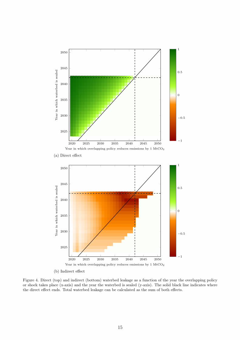
Figure 4. Direct (top) and indirect (bottom) waterbed leakage as a function of the year the overlapping policyor shock takes place (x-axis) and the year the waterbed is sealed (y-axis). The solid black line indicates wherethe direct effect ends. Total waterbed leakage can be calculated as the sum of both effects.

15

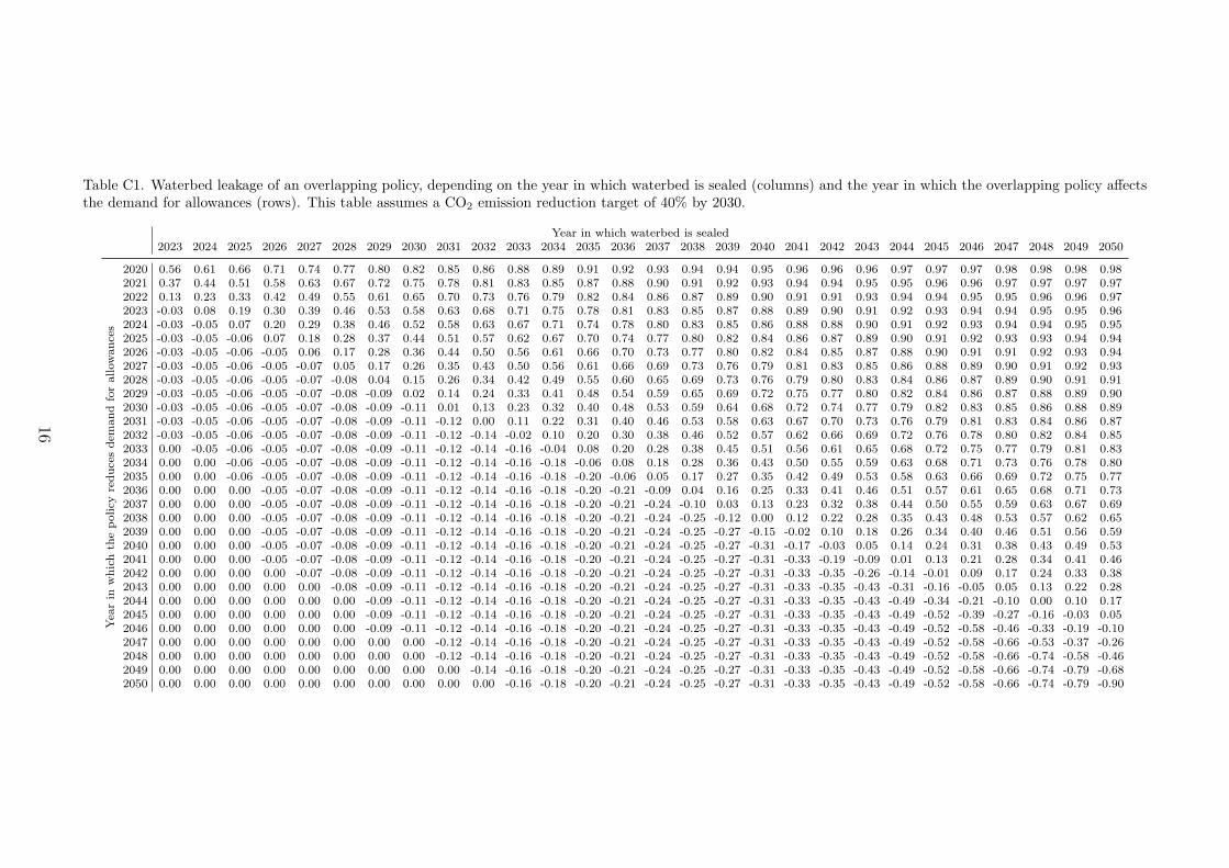
Table C1. Waterbed leakage of an overlapping policy, depending on the year in which waterbed is sealed (columns) and the year in which the overlapping policy affectsthe demand for allowances (rows). This table assumes a CO2 emission reduction target of 40% by 2030.

Year in which waterbed is sealed2023 2024 2025 2026 2027 2028 2029 2030 2031 2032 2033 2034 2035 2036 2037 2038 2039 2040 2041 2042 2043 2044 2045 2046 2047 2048 2049 2050

Yea

rin

whichth

epolicy

reducesdem

andforallowances

2020 0.56 0.61 0.66 0.71 0.74 0.77 0.80 0.82 0.85 0.86 0.88 0.89 0.91 0.92 0.93 0.94 0.94 0.95 0.96 0.96 0.96 0.97 0.97 0.97 0.98 0.98 0.98 0.982021 0.37 0.44 0.51 0.58 0.63 0.67 0.72 0.75 0.78 0.81 0.83 0.85 0.87 0.88 0.90 0.91 0.92 0.93 0.94 0.94 0.95 0.95 0.96 0.96 0.97 0.97 0.97 0.972022 0.13 0.23 0.33 0.42 0.49 0.55 0.61 0.65 0.70 0.73 0.76 0.79 0.82 0.84 0.86 0.87 0.89 0.90 0.91 0.91 0.93 0.94 0.94 0.95 0.95 0.96 0.96 0.972023 -0.03 0.08 0.19 0.30 0.39 0.46 0.53 0.58 0.63 0.68 0.71 0.75 0.78 0.81 0.83 0.85 0.87 0.88 0.89 0.90 0.91 0.92 0.93 0.94 0.94 0.95 0.95 0.962024 -0.03 -0.05 0.07 0.20 0.29 0.38 0.46 0.52 0.58 0.63 0.67 0.71 0.74 0.78 0.80 0.83 0.85 0.86 0.88 0.88 0.90 0.91 0.92 0.93 0.94 0.94 0.95 0.952025 -0.03 -0.05 -0.06 0.07 0.18 0.28 0.37 0.44 0.51 0.57 0.62 0.67 0.70 0.74 0.77 0.80 0.82 0.84 0.86 0.87 0.89 0.90 0.91 0.92 0.93 0.93 0.94 0.942026 -0.03 -0.05 -0.06 -0.05 0.06 0.17 0.28 0.36 0.44 0.50 0.56 0.61 0.66 0.70 0.73 0.77 0.80 0.82 0.84 0.85 0.87 0.88 0.90 0.91 0.91 0.92 0.93 0.942027 -0.03 -0.05 -0.06 -0.05 -0.07 0.05 0.17 0.26 0.35 0.43 0.50 0.56 0.61 0.66 0.69 0.73 0.76 0.79 0.81 0.83 0.85 0.86 0.88 0.89 0.90 0.91 0.92 0.932028 -0.03 -0.05 -0.06 -0.05 -0.07 -0.08 0.04 0.15 0.26 0.34 0.42 0.49 0.55 0.60 0.65 0.69 0.73 0.76 0.79 0.80 0.83 0.84 0.86 0.87 0.89 0.90 0.91 0.912029 -0.03 -0.05 -0.06 -0.05 -0.07 -0.08 -0.09 0.02 0.14 0.24 0.33 0.41 0.48 0.54 0.59 0.65 0.69 0.72 0.75 0.77 0.80 0.82 0.84 0.86 0.87 0.88 0.89 0.902030 -0.03 -0.05 -0.06 -0.05 -0.07 -0.08 -0.09 -0.11 0.01 0.13 0.23 0.32 0.40 0.48 0.53 0.59 0.64 0.68 0.72 0.74 0.77 0.79 0.82 0.83 0.85 0.86 0.88 0.892031 -0.03 -0.05 -0.06 -0.05 -0.07 -0.08 -0.09 -0.11 -0.12 0.00 0.11 0.22 0.31 0.40 0.46 0.53 0.58 0.63 0.67 0.70 0.73 0.76 0.79 0.81 0.83 0.84 0.86 0.872032 -0.03 -0.05 -0.06 -0.05 -0.07 -0.08 -0.09 -0.11 -0.12 -0.14 -0.02 0.10 0.20 0.30 0.38 0.46 0.52 0.57 0.62 0.66 0.69 0.72 0.76 0.78 0.80 0.82 0.84 0.852033 0.00 -0.05 -0.06 -0.05 -0.07 -0.08 -0.09 -0.11 -0.12 -0.14 -0.16 -0.04 0.08 0.20 0.28 0.38 0.45 0.51 0.56 0.61 0.65 0.68 0.72 0.75 0.77 0.79 0.81 0.832034 0.00 0.00 -0.06 -0.05 -0.07 -0.08 -0.09 -0.11 -0.12 -0.14 -0.16 -0.18 -0.06 0.08 0.18 0.28 0.36 0.43 0.50 0.55 0.59 0.63 0.68 0.71 0.73 0.76 0.78 0.802035 0.00 0.00 -0.06 -0.05 -0.07 -0.08 -0.09 -0.11 -0.12 -0.14 -0.16 -0.18 -0.20 -0.06 0.05 0.17 0.27 0.35 0.42 0.49 0.53 0.58 0.63 0.66 0.69 0.72 0.75 0.772036 0.00 0.00 0.00 -0.05 -0.07 -0.08 -0.09 -0.11 -0.12 -0.14 -0.16 -0.18 -0.20 -0.21 -0.09 0.04 0.16 0.25 0.33 0.41 0.46 0.51 0.57 0.61 0.65 0.68 0.71 0.732037 0.00 0.00 0.00 -0.05 -0.07 -0.08 -0.09 -0.11 -0.12 -0.14 -0.16 -0.18 -0.20 -0.21 -0.24 -0.10 0.03 0.13 0.23 0.32 0.38 0.44 0.50 0.55 0.59 0.63 0.67 0.692038 0.00 0.00 0.00 -0.05 -0.07 -0.08 -0.09 -0.11 -0.12 -0.14 -0.16 -0.18 -0.20 -0.21 -0.24 -0.25 -0.12 0.00 0.12 0.22 0.28 0.35 0.43 0.48 0.53 0.57 0.62 0.652039 0.00 0.00 0.00 -0.05 -0.07 -0.08 -0.09 -0.11 -0.12 -0.14 -0.16 -0.18 -0.20 -0.21 -0.24 -0.25 -0.27 -0.15 -0.02 0.10 0.18 0.26 0.34 0.40 0.46 0.51 0.56 0.592040 0.00 0.00 0.00 -0.05 -0.07 -0.08 -0.09 -0.11 -0.12 -0.14 -0.16 -0.18 -0.20 -0.21 -0.24 -0.25 -0.27 -0.31 -0.17 -0.03 0.05 0.14 0.24 0.31 0.38 0.43 0.49 0.532041 0.00 0.00 0.00 -0.05 -0.07 -0.08 -0.09 -0.11 -0.12 -0.14 -0.16 -0.18 -0.20 -0.21 -0.24 -0.25 -0.27 -0.31 -0.33 -0.19 -0.09 0.01 0.13 0.21 0.28 0.34 0.41 0.462042 0.00 0.00 0.00 0.00 -0.07 -0.08 -0.09 -0.11 -0.12 -0.14 -0.16 -0.18 -0.20 -0.21 -0.24 -0.25 -0.27 -0.31 -0.33 -0.35 -0.26 -0.14 -0.01 0.09 0.17 0.24 0.33 0.382043 0.00 0.00 0.00 0.00 0.00 -0.08 -0.09 -0.11 -0.12 -0.14 -0.16 -0.18 -0.20 -0.21 -0.24 -0.25 -0.27 -0.31 -0.33 -0.35 -0.43 -0.31 -0.16 -0.05 0.05 0.13 0.22 0.282044 0.00 0.00 0.00 0.00 0.00 0.00 -0.09 -0.11 -0.12 -0.14 -0.16 -0.18 -0.20 -0.21 -0.24 -0.25 -0.27 -0.31 -0.33 -0.35 -0.43 -0.49 -0.34 -0.21 -0.10 0.00 0.10 0.172045 0.00 0.00 0.00 0.00 0.00 0.00 -0.09 -0.11 -0.12 -0.14 -0.16 -0.18 -0.20 -0.21 -0.24 -0.25 -0.27 -0.31 -0.33 -0.35 -0.43 -0.49 -0.52 -0.39 -0.27 -0.16 -0.03 0.052046 0.00 0.00 0.00 0.00 0.00 0.00 -0.09 -0.11 -0.12 -0.14 -0.16 -0.18 -0.20 -0.21 -0.24 -0.25 -0.27 -0.31 -0.33 -0.35 -0.43 -0.49 -0.52 -0.58 -0.46 -0.33 -0.19 -0.102047 0.00 0.00 0.00 0.00 0.00 0.00 0.00 0.00 -0.12 -0.14 -0.16 -0.18 -0.20 -0.21 -0.24 -0.25 -0.27 -0.31 -0.33 -0.35 -0.43 -0.49 -0.52 -0.58 -0.66 -0.53 -0.37 -0.262048 0.00 0.00 0.00 0.00 0.00 0.00 0.00 0.00 -0.12 -0.14 -0.16 -0.18 -0.20 -0.21 -0.24 -0.25 -0.27 -0.31 -0.33 -0.35 -0.43 -0.49 -0.52 -0.58 -0.66 -0.74 -0.58 -0.462049 0.00 0.00 0.00 0.00 0.00 0.00 0.00 0.00 0.00 -0.14 -0.16 -0.18 -0.20 -0.21 -0.24 -0.25 -0.27 -0.31 -0.33 -0.35 -0.43 -0.49 -0.52 -0.58 -0.66 -0.74 -0.79 -0.682050 0.00 0.00 0.00 0.00 0.00 0.00 0.00 0.00 0.00 0.00 -0.16 -0.18 -0.20 -0.21 -0.24 -0.25 -0.27 -0.31 -0.33 -0.35 -0.43 -0.49 -0.52 -0.58 -0.66 -0.74 -0.79 -0.90

16

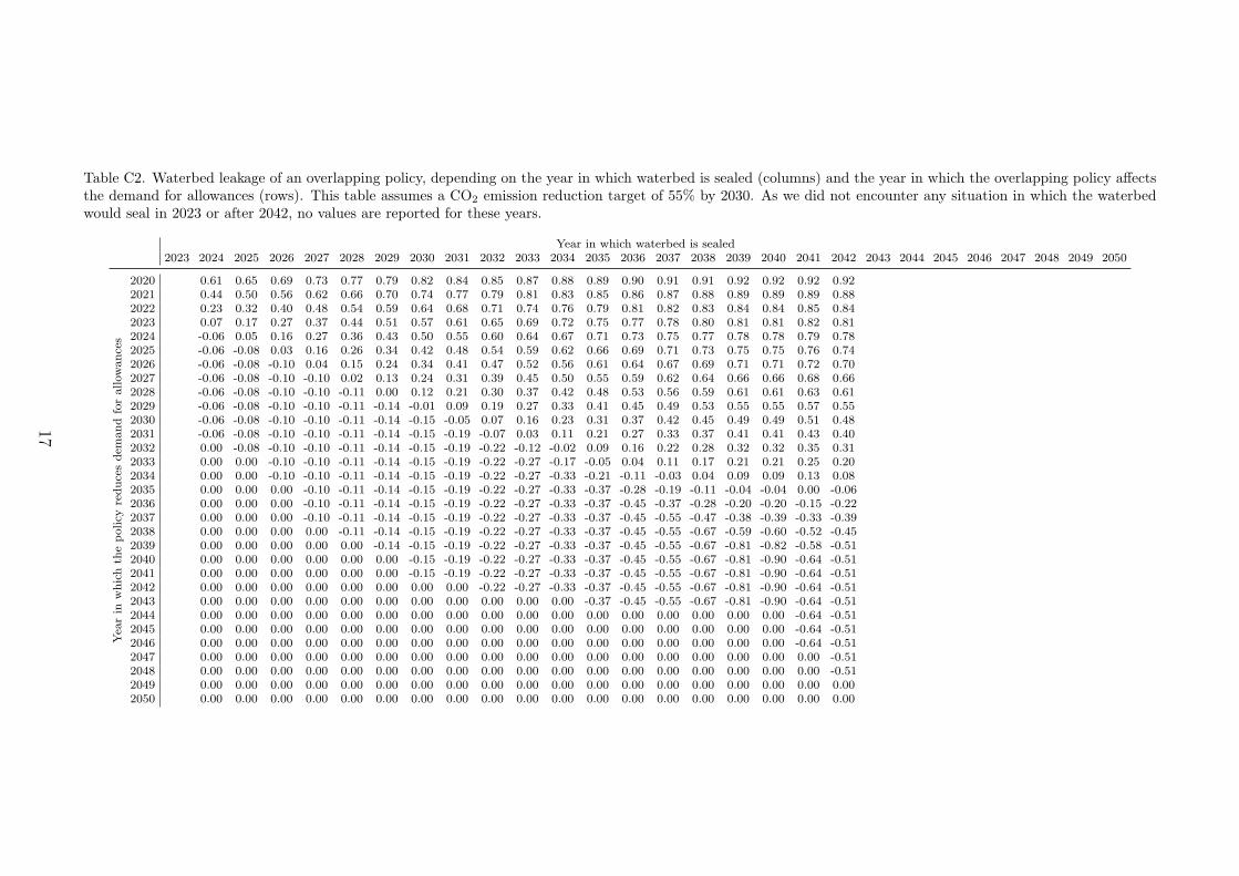
Table C2. Waterbed leakage of an overlapping policy, depending on the year in which waterbed is sealed (columns) and the year in which the overlapping policy affectsthe demand for allowances (rows). This table assumes a CO2 emission reduction target of 55% by 2030. As we did not encounter any situation in which the waterbedwould seal in 2023 or after 2042, no values are reported for these years.

Year in which waterbed is sealed2023 2024 2025 2026 2027 2028 2029 2030 2031 2032 2033 2034 2035 2036 2037 2038 2039 2040 2041 2042 2043 2044 2045 2046 2047 2048 2049 2050

Yea

rin

whichth

epolicy

reducesdem

andforallowances

2020 0.61 0.65 0.69 0.73 0.77 0.79 0.82 0.84 0.85 0.87 0.88 0.89 0.90 0.91 0.91 0.92 0.92 0.92 0.922021 0.44 0.50 0.56 0.62 0.66 0.70 0.74 0.77 0.79 0.81 0.83 0.85 0.86 0.87 0.88 0.89 0.89 0.89 0.882022 0.23 0.32 0.40 0.48 0.54 0.59 0.64 0.68 0.71 0.74 0.76 0.79 0.81 0.82 0.83 0.84 0.84 0.85 0.842023 0.07 0.17 0.27 0.37 0.44 0.51 0.57 0.61 0.65 0.69 0.72 0.75 0.77 0.78 0.80 0.81 0.81 0.82 0.812024 -0.06 0.05 0.16 0.27 0.36 0.43 0.50 0.55 0.60 0.64 0.67 0.71 0.73 0.75 0.77 0.78 0.78 0.79 0.782025 -0.06 -0.08 0.03 0.16 0.26 0.34 0.42 0.48 0.54 0.59 0.62 0.66 0.69 0.71 0.73 0.75 0.75 0.76 0.742026 -0.06 -0.08 -0.10 0.04 0.15 0.24 0.34 0.41 0.47 0.52 0.56 0.61 0.64 0.67 0.69 0.71 0.71 0.72 0.702027 -0.06 -0.08 -0.10 -0.10 0.02 0.13 0.24 0.31 0.39 0.45 0.50 0.55 0.59 0.62 0.64 0.66 0.66 0.68 0.662028 -0.06 -0.08 -0.10 -0.10 -0.11 0.00 0.12 0.21 0.30 0.37 0.42 0.48 0.53 0.56 0.59 0.61 0.61 0.63 0.612029 -0.06 -0.08 -0.10 -0.10 -0.11 -0.14 -0.01 0.09 0.19 0.27 0.33 0.41 0.45 0.49 0.53 0.55 0.55 0.57 0.552030 -0.06 -0.08 -0.10 -0.10 -0.11 -0.14 -0.15 -0.05 0.07 0.16 0.23 0.31 0.37 0.42 0.45 0.49 0.49 0.51 0.482031 -0.06 -0.08 -0.10 -0.10 -0.11 -0.14 -0.15 -0.19 -0.07 0.03 0.11 0.21 0.27 0.33 0.37 0.41 0.41 0.43 0.402032 0.00 -0.08 -0.10 -0.10 -0.11 -0.14 -0.15 -0.19 -0.22 -0.12 -0.02 0.09 0.16 0.22 0.28 0.32 0.32 0.35 0.312033 0.00 0.00 -0.10 -0.10 -0.11 -0.14 -0.15 -0.19 -0.22 -0.27 -0.17 -0.05 0.04 0.11 0.17 0.21 0.21 0.25 0.202034 0.00 0.00 -0.10 -0.10 -0.11 -0.14 -0.15 -0.19 -0.22 -0.27 -0.33 -0.21 -0.11 -0.03 0.04 0.09 0.09 0.13 0.082035 0.00 0.00 0.00 -0.10 -0.11 -0.14 -0.15 -0.19 -0.22 -0.27 -0.33 -0.37 -0.28 -0.19 -0.11 -0.04 -0.04 0.00 -0.062036 0.00 0.00 0.00 -0.10 -0.11 -0.14 -0.15 -0.19 -0.22 -0.27 -0.33 -0.37 -0.45 -0.37 -0.28 -0.20 -0.20 -0.15 -0.222037 0.00 0.00 0.00 -0.10 -0.11 -0.14 -0.15 -0.19 -0.22 -0.27 -0.33 -0.37 -0.45 -0.55 -0.47 -0.38 -0.39 -0.33 -0.392038 0.00 0.00 0.00 0.00 -0.11 -0.14 -0.15 -0.19 -0.22 -0.27 -0.33 -0.37 -0.45 -0.55 -0.67 -0.59 -0.60 -0.52 -0.452039 0.00 0.00 0.00 0.00 0.00 -0.14 -0.15 -0.19 -0.22 -0.27 -0.33 -0.37 -0.45 -0.55 -0.67 -0.81 -0.82 -0.58 -0.512040 0.00 0.00 0.00 0.00 0.00 0.00 -0.15 -0.19 -0.22 -0.27 -0.33 -0.37 -0.45 -0.55 -0.67 -0.81 -0.90 -0.64 -0.512041 0.00 0.00 0.00 0.00 0.00 0.00 -0.15 -0.19 -0.22 -0.27 -0.33 -0.37 -0.45 -0.55 -0.67 -0.81 -0.90 -0.64 -0.512042 0.00 0.00 0.00 0.00 0.00 0.00 0.00 0.00 -0.22 -0.27 -0.33 -0.37 -0.45 -0.55 -0.67 -0.81 -0.90 -0.64 -0.512043 0.00 0.00 0.00 0.00 0.00 0.00 0.00 0.00 0.00 0.00 0.00 -0.37 -0.45 -0.55 -0.67 -0.81 -0.90 -0.64 -0.512044 0.00 0.00 0.00 0.00 0.00 0.00 0.00 0.00 0.00 0.00 0.00 0.00 0.00 0.00 0.00 0.00 0.00 -0.64 -0.512045 0.00 0.00 0.00 0.00 0.00 0.00 0.00 0.00 0.00 0.00 0.00 0.00 0.00 0.00 0.00 0.00 0.00 -0.64 -0.512046 0.00 0.00 0.00 0.00 0.00 0.00 0.00 0.00 0.00 0.00 0.00 0.00 0.00 0.00 0.00 0.00 0.00 -0.64 -0.512047 0.00 0.00 0.00 0.00 0.00 0.00 0.00 0.00 0.00 0.00 0.00 0.00 0.00 0.00 0.00 0.00 0.00 0.00 -0.512048 0.00 0.00 0.00 0.00 0.00 0.00 0.00 0.00 0.00 0.00 0.00 0.00 0.00 0.00 0.00 0.00 0.00 0.00 -0.512049 0.00 0.00 0.00 0.00 0.00 0.00 0.00 0.00 0.00 0.00 0.00 0.00 0.00 0.00 0.00 0.00 0.00 0.00 0.002050 0.00 0.00 0.00 0.00 0.00 0.00 0.00 0.00 0.00 0.00 0.00 0.00 0.00 0.00 0.00 0.00 0.00 0.00 0.00

17

References

Azarova, V., Mier, M., 2020. Market Stability Reserve under exogenous shock: The case ofCOVID-19 pandemic. Applied Energy (December).

Beck, U., Kruse, P. K., 2020. Endogenizing the Cap in a Cap and Trade System : Assessingthe Agreement on EU ETS Phase 4. Vol. 77. Springer Netherlands.URL https://doi.org/10.1007/s10640-020-00518-w

Bertram, C., Luderer, G., Pietzcker, R. C., Schmid, E., Kriegler, E., Edenhofer, O., 2015.Complementing carbon prices with technology policies to keep climate targets within reach.Nature Climate Change 5 (3), 235–239.

Borenstein, S., Bushnell, J., Wolak, F. A., Zaragoza-Watkins, M., 2019. Expecting the Un-expected : Emissions Uncertainty and Environmental Market Design. American EconomicReview (Forthcoming).

Bruninx, K., Ovaere, M., 2020. Estimating the Impact of COVID-19 on Emissions and EmissionAllowance Prices Under EU ETS. Energy Forum (Covid-19 issue), 40–42.

Bruninx, K., Ovaere, M., Delarue, E., 2020. The long-term impact of the market stabilityreserve on the EU emission trading system. Energy Economics 89 (June).

Bruninx, K., Ovaere, M., Gillingham, K., Delarue, E., 2019. The unintended con-sequences of the eu ets cancellation policy. KU Leuven Energy Institute Work-ing Paper EN2019-11. Available online: www.mech.kuleuven.be/en/tme/research/

energy-systems-integration-modeling/publications.

Creutzig, F., Agoston, P., Goldschmidt, J. C., Luderer, G., Nemet, G., Pietzcker, R. C., 2017.The underestimated potential of solar energy to mitigate climate change. Nature Energy2 (9), 1–9.

EEX, Last accessed: April 1, 2020. Emission Spot Primary Market Auction Re-port. Available online: https://www.eex.com/en/products/environmental-markets/

emissions-auctions/archive.

European Commission, 2019. Communication from the Commission. Publication of the totalnumber of allowances in circulation in 2018 for the purposes of the Market Stability Reserveunder the EU Emissions Trading System established by Directive 2003/87/EC. Tech. Report.Brussels, Belgium.

European Commission, 2020a. Publication of the total number of allowances in circulationin 2019 for the purposes of the Market Stability Reserve under the EU Emissions TradingSystem established by Directive 2003/87/EC. Tech. rep.

European Commission, 2020b. State of the Union: Commission raises climate ambition andproposes 55% cut in emissions by 2030. Tech. rep.

European Union, 2018. Directive (EU) 2018/410 of the European Parliament and the Council of14 March 2018 amending Directive 2003/87/EC to enhance cost-effective emission reductionsand low-carbon investments, and Decision (EU) 2015/1814. Official Journal of the EuropeanUnion 76, 3–27.

Gerlagh, R., Heijmans, J., 2019. Climate-conscious consumers and the buy, bank, burn program.Nature Climate Change 9 (June), 431–433.

18

Gerlagh, R., Heijmans, R. J. R. K., Rosendahl, K. E., 2020a. COVID 19 Tests the MarketStability Reserve. Environmental and Resource Economics 76 (4), 855–865.URL https://doi.org/10.1007/s10640-020-00441-0

Gerlagh, R., Heijmans, R. J. R. K., Rosendahl, K. E., 2020b. Endogenous Emission CapsAlways Produce a Green Paradox.

Gillingham, K. T., Knittel, C. R., Li, J., Ovaere, M., Reguant, M., 2020. The short-run andlong-run effects of covid-19 on energy and the environment. Joule 4 (7), 1337–1341.

Hintermayer, M., Schmidt, L., Zinke, J., 2020. On the time-dependency of MAC curves and itsimplications for the EU ETS.

Koch, N., Fuss, S., Grosjean, G., Edenhofer, O., 2014. Causes of the EU ETS price drop:Recession, CDM, renewable policies or a bit of everything?-New evidence. Energy Policy 73,676–685.

Landis, F., 2015. Final report on marginal abatement cost curves for the evaluation of themarket stability reserve. ZEW-Dokumentation No. 15-01.

Le Quere, C., Jackson, R. B., Jones, M. W., Smith, A. J., Abernethy, S., Andrew, R. M.,De-Gol, A. J., Willis, D. R., Shan, Y., Canadell, J. G., et al., 2020. Temporary reduction indaily global co 2 emissions during the covid-19 forced confinement. Nature Climate Change,1–7.

Liu, Z., Ciais, P., Deng, Z., Lei, R., Davis, S. J., Feng, S., Zheng, B., Cui, D., Dou, X., Zhu,B., et al., 2020. Near-real-time monitoring of global co 2 emissions reveals the effects of thecovid-19 pandemic. Nature communications 11 (1), 1–12.

Perino, G., 2018. New EU ETS Phase 4 rules temporarily puncture waterbed. Nature ClimateChange 8 (4), 262–264.

Perino, G., Pahle, M., Pause, F., Quemin, S., Scheuing, H., 2021. EU ETS stability mechanismneeds new design (2018), 1–15.

Perino, G., Ritz, R. A., Benthem, A. A. V., 2020. Overlapping Climate Policies 1 (215), 1–54.

Perino, G., Willner, M., 2017. EU-ETS Phase IV: allowance prices, design choices and themarket stability reserve. Climate Policy 17 (7), 936–946.

Quemin, S., Trotignon, R., 2019. Emissions Trading with Rolling Horizons.

Rosendahl, K. E., 2019a. Eu ets and the new green paradox. NMBU Working Papers No.2/2019.

Rosendahl, K. E., 2019b. EU ETS and the waterbed effect. Nature Climate Change 9 (734),734–735.

19

Figures

Figure 1

Waterbed leakage (the net effect of a shock or overlapping policy on cumulative emissions in EU ETS) asa function of the year the overlapping policy or shock takes place (horizontal axis) and the year thewaterbed is sealed (vertical axis). The solid black line indicates where the direct effect ends. Waterbed

leakage is positive when a policy that increases (decreases) emissions leads to increased (decreased)cumulative emissions. It is negative when a policy back res. Note that we ignore the possibility thatoverlapping policies affect the duration of the punctured waterbed. The numerical values behind thesegraphs are reported in Appendix C, alongside with a separate graphical representation of the direct andindirect effect.

Figure 2

Cumulative emissions (a) and allowances prices (b) in each of our six scenarios. The black and grey barsrepresent the range of outcomes, the white markers represent the median value and the vertical red linesrepresent the cumulative cap without cancellation (2020-end ETS). The indicated years are the years inwhich the waterbed is sealed in the edge cases (lowest-highest emissions). The cumulative impact ofCOVID-19 pandemic is assumed to be 0.72 GtCO2 in the period 2020-2025 and is enforced in allscenarios except the "No pandemic" scenario. Scenario (3) and (5) mimic the effect of an overlappingpolicy reducing (3) or increasing (5) emissions by 100 MtCO2/year in the period 2021-2031, consideringthe -55% emission reduction target.

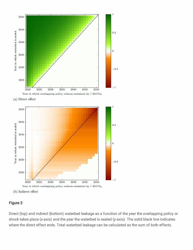
Figure 3

Direct (top) and indirect (bottom) waterbed leakage as a function of the year the overlapping policy orshock takes place (x-axis) and the year the waterbed is sealed (y-axis). The solid black line indicateswhere the direct effect ends. Total waterbed leakage can be calculated as the sum of both effects.

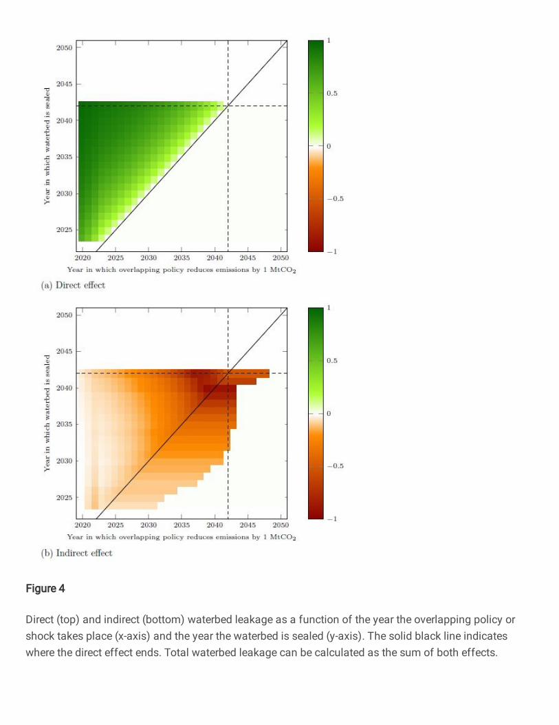
Figure 4

Direct (top) and indirect (bottom) waterbed leakage as a function of the year the overlapping policy orshock takes place (x-axis) and the year the waterbed is sealed (y-axis). The solid black line indicateswhere the direct effect ends. Total waterbed leakage can be calculated as the sum of both effects.