water urbanism: building more coherent cities
TRANSCRIPT

WATER URBANISM: BUILDING MORE COHERENT CITIES
by
HOPE HUI RISING
A DISSERTATION
Presented to the Department of Landscape Architecture
and the Graduate School of the University of Oregon
in partial fulfillment of the requirements
for the degree of
Doctor of Philosophy
June 2015

ii
DISSERTATION APPROVAL PAGE
Student: Hope Hui Rising
Title: Water Urbanism: Building More Coherent Cities
This dissertation has been accepted and approved in partial fulfillment of the
requirements for the Doctor of Philosophy degree in the Department of Landscape
Architecture by:
Robert Ribe Chairperson
Amy Lobben Core Member
Deni Ruggeri Core Member
Elliot Berkman Institutional Representative
and
Scott L. Pratt Dean of the Graduate School
Original approval signatures are on file with the University of Oregon Graduate School.
Degree awarded June 2015

iii
© 2015 Hope Hui Rising

iv
DISSERTATION ABSTRACT
Hope Hui Rising
Doctor of Philosophy
Department of Landscape Architecture
June 2015
Title: Water Urbanism: Building More Coherent Cities
A more water-coherent approach is postulated as a primary pathway through which
biophilic urbanism contributes to livability and climate change adaptation. Previous studies
have shown that upstream water retention is more cost-effective than downstream for
mitigating flood risks downstream. This dissertation proposes a research design for
generating an iconography of water urbanism to make upstream cities more coherent. I
tested a hypothesis of aquaphilic urbanism as a water-based sense of place that evokes
water-based place attachment to help adapt cities and individuals to water-coherent
urbanism.
Cognitive mapping, photovoice, and emotional recall protocols were conducted
during semi‐structured interviews with 60 residents and visitors sampled from eight water-
centric cities in the Netherlands, Germany, and Belgium. The participants provided 55
sketch maps. I performed content analyses, regression analyses, path analyses, and
mediation analyses to study the relationships of 1) pictorial aquaphilia (intrinsic attachment
to safe and clean water scenes) and waterscape imageability, 2) waterscape imageability
and the coherence of city image, 3) egocentric aquaphilia (attachment to water-based
spatial anchors) and allocentric aquaphilia (attachment to water-centric cities), and 4) the
coherence of city image, allocentric aquaphilia, and openness towards water-coherent

v
urbanism.
Content analyses show that waterscape imageability and pictorial aquaphilia were
the two most common reasons why participants mentioned the five waterscape types,
including water landmarks, canals, lakes, rivers, and harbors, during the three recall
protocols. Regression analyses indicate that water is a sixth element of imageability and
that the imageable structure of canals and rivers and the identifiability of water landmarks
significantly influenced the aesthetic coherence of city image. Path analyses suggest that
allocentric aquaphilia can be attributed to water-based familiarity, water-based place
identity (or identifiability), water-based comfort, and water-based place dependence (or
orientation) evoked by water-based spatial anchors. Mediation analyses reveal that water-
based goal affordance (as a construct of water-based comfort and water-based place
dependence) aided environmental adaptation, while water-based imageability (as a
construct of water-based familiarity and water-based place identity) helped adapt cities and
individuals to water-coherent urbanism. Canal mappability mediated the effects of gender
and of visitor versus resident on the coherence of city image to facilitate environmental
adaptation.

vi
CURRICULUM VITAE
NAME OF AUTHOR: Hope Hui Rising
GRADUATE AND UNDERGRADUATE SCHOOLS ATTENDED:
University of Oregon, Eugene
University of Michigan, Ann Arbor
National Taiwan University, Taipei
DEGREES AWARDED:
Doctor of Philosophy in Landscape Architecture, 2015, University of Oregon
Master of Landscape Architecture, 2000, University of Michigan
Master of Urban Planning, 2000, University of Michigan
Bachelor of Science in Engineering, 1996, National Taiwan University
AREAS OF SPECIAL INTEREST:
Public realm planning and design, water and ecological planning and design,
human aspects of environmental design, participatory design, water-sensitive
urban design
PROFESSIONAL EXPERIENCE:
Co-Instructor, Intermediate Design Studio, Department of Landscape
Architecture, University of Oregon, Spring 2015
Graduate Research Fellow, Informational Effect on Forest Perception,
Department of Landscape Architecture, University of Oregon, Spring 2014
Graduate Research Fellow, Medieval and Contemporary Science Gardens,
Department of Landscape Architecture, University of Oregon, Spring 2014
Co-Instructor, Undergraduate and Graduate Urban Design Terminal Studio,
Department of Architecture, University of Oregon, Winter 2014
Graduate Research Fellow, Urban Design Lab, University of Oregon, Spring 2013
Co-Instructor, Undergraduate Landscape Architecture Terminal Studio,
Department of Landscape Architecture, University of Oregon, Winter 2013
Roving Critic, Department of Landscape Architecture, Winter 2013
Instructor, Transformative Spaces Elective, Department of Landscape
Architecture and Department of Dance, University of Oregon, Spring 2012

vii
Partner, BioNova, 2012-2013
Research Assistant, Visual Neuroscience Lab, University of Oregon, 2011-2012
Research Assistant, Brain Electrophysiology Lab, University of Oregon, 2011-
2012
Director, Om Creation Studio, LLC, 2007-2013
Studio Lead Designer, Urban Design and Landscape Architecture Studio, HOK
Architecture & Planning New York Office, 2006-2007
Project Lead Designer and Manager, Design Studio, EDAW, Inc., Alexandria
Office, 2001-2006
Graduate Student Instructor, Site Planning and Engineering, Department of
Architecture, University of Michigan, Fall 2000
Landscape Architecture Intern, Design Studio, EDAW, Inc., Alexandria Office,
Summer 2000
Graduate Student Instructor, Landscape Ecology Design Studio, Department of
Landscape Architecture, University of Michigan, Spring 2000
Landscape Architecture Intern, Washtenaw Engineering Company, 1998-1999
Research Assistant, University of Michigan Transportation Research
Institute, 1998-1999
Survey Manager, Ann Arbor Area Transportation Authority/Department of Urban
and Regional Planning, University of Michigan, Summer, 1998
Research Assistant, Urban Security Group, University of Michigan, Fall 1997
GRANTS, AWARDS, AND HONORS:
Research Grant, Environmental Design Research Association, 2014-2015
Ministry of Education Scholarship, TECO, San Francisco, CA 2013-2015
Conference Scholarship, Environmental Design Research Association, 2014
Ph.D. Development Fund, Department of Landscape Architecture, University of
Oregon, 2014
Ph.D. Development Fund, Department of Landscape Architecture, University of
Oregon, 2013
Graduate (Dissertation) Research Fellowship, Department of Landscape
Architecture, University of Oregon, Fall 2013, Fall 2014, and Winter 2015
Gary Smith Summer Development Award, University of Oregon, 2012
Conference Scholarship, Environmental Design Research Association, 2012
Cluster Fellowship, International Smart Geometry Conference, 2012
International Finalist, the Union Colony Civic Center Public Art & Water Feature,
Greeley, CO, 2012 (Lead Designer and Public Artist with Om Creation Studio)
Promising Scholar Award, University of Oregon, 2011-2013
Berger Scholarship, Department of Landscape Architecture, University of
Oregon, 2011
One Percent Green Recipient, Portland Bureau of Environmental Services, 2010
(Lead Landscape Architect and Public Artist with Om Creation Studio)

viii
Conference Fellowship, Rail-Volution, Livable Portland, 2010
National Winner, Dorothy’s Place Public Art, Public Art St. Paul, 2010 (Lead
Landscape Architect and Public Artist with Om Creation Studio)
Cultural STAR Grant, St. Paul City Council, 2010 (Lead Landscape Architect and
Public Artist with Om Creation Studio)
Hankyung Grand Prize, New Songdo Central Park I Block 22, Incheon, Korea,
2009 (Lead Landscape Architect and Public Artist with HOK)
Potomac ASLA Honor Award, World of Wonders Children’s Garden, Norfolk,
VA, 2008 (Project Lead Designer and Manager with EDAW)
Maryland ASLA Honor Award, World of Wonders Children’s Garden, Norfolk,
VA, 2008 (Project Lead Designer and Manager with EDAW)
Potomac ASLA Honor Award, Wharf District Park, Boston, MA, 2008
(Project Designer and Assistant Project Manager with EDAW)
Northern Virginia AIA Merit Award, SallieMae Headquarters, Reston, VA, 2007
(Project Designer with EDAW)
Durham City-County Golden Leaf Merit Award for Community Properties,
Museum of Life and Science “Explore the Wild” Exhibit, Durham, NC, 2007
(Project Lead Designer and Manager with EDAW)
National Winner, Arverne East Oceanfront Development Competition,
New York Housing Preservation and Development, Queens, New York, 2006
(Lead Landscape Architect with HOK)
Carolinas Pinnacle Award, Museum of Life and Science, Durham, NC, 2006
(Project Lead Designer and Manager with EDAW)
Potomac Valley AIA Grand Honor Award, Katzen Arts Center at American
University, D.C., 2005 (Project Designer and Manager with EDAW)
Washington D.C. AIA Merit Award, Katzen Arts Center at American University,
D.C., 2005 (Project Designer and Manager with EDAW)
Inform Award of Honor for Landscape Architecture, Katzen Arts Center at
American University, D.C., 2005 (Project Designer and Manager with
EDAW)
Mid-Atlantic Construction Magazine Design Merit Award for Cultural, Museum,
and Entertainment Category, Katzen Arts Center at American University,
D.C., 2005 (Project Designer and Manager with EDAW)
National Finalist, Veterans Freedom Park Memorial Design Competition, Cary,
NC, 2004 (Lead Designer and Project Manager with EDAW)
International Finalist, Beale Street Landing Competition, Memphis Waterfront
Redevelopment Corporation, Memphis, TN, 2003 (Landscape Architect with
EDAW)
National ASLA Analysis and Planning Merit Award, Michigan Department of
Transportation Aesthetic Project Opportunities Inventory and Scenic Heritage
Route Designation Inventory in Michigan, 2001 (Landscape Architecture
Intern with Washtenaw Engineering Company)
Certificate of Honor, National Landscape Architecture Honor Society, 2000
Barbour Scholar Fellowship, University of Michigan, 1998-1999
Alumni Award, National Taiwan University, Taiwan, 1996
President’s Award, National Taiwan University, Taiwan, 1993-1996

ix
PUBLICATIONS:
Rising, H. (2015). Water urbanism: The influences of aquaphilia on urban
design. Journal of Urban Design. (Revise and Resubmit)
Rising, H. (2014). Placing “blue parkway” in the crosscurrents of water
urbanism. Building with Change: Proceedings of the 45th
Annual Conference
of the Environmental Design Research Association, p.315-316, New Orleans,
LA: Environmental Design Research Association.
Rising, H. (2014). Water-based place attachment: The role of water aesthetics in
adaptation. Building with Change: Proceedings of the 45th Annual
Conference of the Environmental Design Research Association, p.382, New
Orleans, LA: Environmental Design Research Association.
Rising, H. & Ribe, R. (2014). The image of the water city: Designing for
universal place attachment with water-coherent urbanism. Proceedings of the
2014 Council for Educators in Landscape Architecture Conference, p.220.
Baltimore, MD: Council for Educators in Landscape Architecture.
Rising, H. & Gillem, M. (2014). Mainstreaming water urbanism: In search of
public acceptance for urban design interventions as climate change adaptation
and sea level rise mitigation strategies. Proceedings of the 2014 Council for
Educators in Landscape Architecture Conference, p.305. Baltimore, MD:
Council for Educators in Landscape Architecture.

x
ACKNOWLEDGMENTS
This research was funded in part by graduate research fellowships from the
University of Oregon Department of Landscape Architecture, an EDRA research grant,
and a Ministry of Education Scholarship administered through TECO in San Francisco.
My department provided two Ph.D. Development Funds to cover airfare for my fieldwork
and for two presentations at the 2014 Annual CELA Conference. Special thanks also go
to EDRA for providing two conference scholarships to support my travel to the 2012 and
2014 Annual EDRA Conferences for three presentations.
My growth as an academic has been facilitated by an outstanding community of
scholars. Robert Ribe cultivated an incubator for interdisciplinary innovations and
inspired me with his dedication to student-centered education. Deni Ruggeri, Amy
Lobben, and Elliot Berkman brought relevant literature and methods to my attention.
David Hulse and Bart Johnson provided insightful feedback during Ph.D. progress
meetings. Liska Chan thoughtfully orchestrated opportunities for me to hone teaching and
research skills. Robert Melnick motivated me to become a better pedagogue. Kenneth
Helphand showed me how classroom instructions could be elevated into a form of art.
Nancy Chang provided me with opportunities to interact with a cutting-edge digital
media community and exchange scholars.
Mark Gillem, Yizhao Yang, Vicki Elmer, and Patricia Gwartney provided helpful
comments on earlier drafts of my dissertation proposal. David DeGarmo and Mark Van
Ryzin helped increase my data analysis productivity. Don Tucker, Margaret Sereno, and
Richard Taylor helped me gain invaluable hands-on research experience in neuroscience
labs. I am also very thankful for the assistance of my independent raters, Leona Chen,

xi
Nicole Blodgett, Dequah Hussein, and Josette Katcha. The wonderful students in my
department and college inspired me with their refreshing perspectives and dedication to
bettering the world.
The Dutch, Belgian, and German Embassies patiently helped me navigate local
IRB requirements and made me feel very welcome to conduct research in their countries.
Anonymous field participants were extremely generous with their time. Various experts
went beyond their duties to share their expertise: Irene Curulli (Eindhoven University of
Technology), Quinten Niessen (Municipal Water District of Central Amsterdam), Wouter
van de Veur (Amsterdam Department of Physical Planning and Policy Team), Reinier
Nijland (City of Almere), Han Meyer (Delft University), Jorg Pieneman (Rotterdam
Bureau of Water Management), Gloria Font (Amsterdam Academy of Architecture), and
Michelle Provoost and Han van Beusekom (International New Town Institute).
Many friends made me feel at home during my research trip. In Berlin, Isa hosted
me, Peter shared his local knowledge, and George organized a restaurant gathering with
friends. Gabrella shared her expertise in water and wetland management, and Rhoda
drove me around Giethoorn. Werner and Gervais assisted me in Ghent and Bruges. I am
grateful for my great grandfather, a landscape contractor known as “the waterman,” for
exposing me to landscape architecture, and my great grandmother for telling me many
stories about the waterways that used to exist during the Japanese Occupation. I am very
thankful for my parents for providing me with the opportunities to transcend cultural
boundaries. My deepest appreciation is due to two angels, Ben and Elias, for helping me
move many times, picking up household chores, and catering to my demanding
schedules. They made a tremendous personal sacrifice to uproot themselves to follow me.
xii
TABLE OF CONTENTS
Chapter Page
I. COHERENT URBANISM THROUGH WATER URBANISM ............................. 1
Definition of Terms................................................................................................ 1
Aquaphilia and Water Urbanism ..................................................................... 1
Water Urbanism and Aquaphilic Urbanism ..................................................... 1
Aquaphilia and Biophilia ................................................................................. 2
Behavioral and Structural Interpretations of Aquaphilia ................................. 2
Water-Resistant and Water-Coherent Urbanisms ............................................ 3
Background ............................................................................................................ 3
Projected Increase in Climate Refugee Population .......................................... 3
Environmental Adaptation of Voluntary Migrants in Safer Locations ............ 4
Mismatch of Jobs and Populations for Water Amenity-Driven Voluntary
Migration.................................................................................................... 4
Positive Pull and Negative Push Factors of Environmental Preference .......... 6
A Growing Need for Upstream Water-Retention ............................................ 6
A Water-Coherent Impetus in Green Infrastructure Movement ...................... 7
An Emerging Water-Coherent Urbanism for Upstream and Inland Cities ...... 8
The Image of the Water City ........................................................................... 8
Aquaphilia as the Function of Aesthetic Coherence in Adaptation ................. 9
Allocentric and Egocentric Perspectives of Aesthetic Coherence ................... 9
Aesthetic Coherence from the Picturesque Tradition ...................................... 10
An Urban Picturesque Theory of Emotional Coherence ................................. 11

xiii
Chapter Page
In Search of a Postmodern Urban Design Experiment .................................... 12
Determinism as Conundrum of Designing an Emancipating Public Realm .... 12
Lessons Learned from Previous Postmodern Urban Design Experiments ...... 15
Mainstreaming Urban Design Experiments with City Image Coherence ........ 16
Water-Coherent Urbanism – a Promising Form of Coherent Urbanism ......... 19
Study Objectives .................................................................................................... 20
Project Significance ............................................................................................... 20
Site Selection ......................................................................................................... 21
Chapter Descriptions .............................................................................................. 21
Chapter I – Coherent Urbanism Through Water Urbanism ............................. 21
Chapter II – Water Urbanism: The Influences of Aquaphilia on Urban
Design ........................................................................................................ 22
Chapter III – The Image of the Water City: Testing the Imageability
Theory for Structuring the Pluralistic Water City ...................................... 23
Chapter IV – Aquaphilic Urbanism: Water-Based Spatial Anchors as
Loci of Attachment .................................................................................... 25
Chapter V – Aquaphilia: The Function of Aquaphilic Urbanism for
Adaptation .................................................................................................. 27
Chapter VI – Toward an Iconography of Water Urbanism ............................. 28
Interrelationships Among Chapters Reporting Empirical Investigations ....... 29

xiv
Chapter Page
II. WATER URBANISM: THE INFLUENCES OF AQUAPHILIA ON URBAN
DESIGN ................................................................................................................. 33
Introduction ............................................................................................................ 33
Aquaphilia as a Timeless Concept ................................................................... 33
From Biophilic Urbanism to Aquaphilic Urbanism ......................................... 33
Project Objective .............................................................................................. 34
Literature Review................................................................................................... 34
In Search of an Aesthetic Discourse for Green Infrastructure ......................... 34
The Effects of Water’s Presence on Perception of Green Infrastructure ......... 35
Green Infrastructure as Locus of Attachment Due to Comfort ........................ 35
Green Infrastructure as a Spatial Anchor and Contributor to Attachment ....... 36
The Affordances of Green Infrastructure as a Locus of Attachment ............... 36
Coherence as an Urban Picturesque Concept .................................................. 37
Pictorial Coherence .................................................................................... 38
Egocentric Coherence ................................................................................ 38
Allocentric Coherence ............................................................................... 39
Emotional Coherence ................................................................................. 39
Research Design ..................................................................................................... 40
Site Selection .................................................................................................. 40
Data Collection ................................................................................................ 40
Analytical Framework ..................................................................................... 41
Descriptors of Urban Design Quality ........................................................ 41

xv
Chapter Page
Urban Design Attributes Based on Affordance Types .............................. 41
Data Analysis for Likes and Dislikes about Water Networks ............................... 43
Recall Sequence as an Emotional Salience Indicator ...................................... 43
Results and Discussions for Likes and Dislikes about Water Networks ............... 44
Urban Design Attributes as Contributors to Likes and Dislikes ...................... 44
Negative Influence from the Threats to Pictorial Aquaphilia .......................... 47
Intrinsic Urban Design Quality of Egocentric Aquaphilia .............................. 48
Data Analysis for Cognitive Mapping and Photovoice ......................................... 49
Waterscape Types Based on Elements of Imageability ................................... 49
Recall Sequence as an Indicator of Spatial Anchor Salience .......................... 50
Urban Design Attributes as Contributors to Waterscape Salience .................. 50
Results and Discussions for Cognitive Mapping ................................................... 50
Contribution of Imageability to Waterscape Allocentric Salience .................. 50
Dual-View Nature of Spatial Knowledge in Cognitive Maps ......................... 54
Waterscape Imageability and Urban Design Implications ............................... 55
Aquaphilia’s Influence on Allocentric Salience of Waterscapes ..................... 55
Accessibility’s Influence on Allocentric Salience of Waterscapes .................. 56
Canals, Rivers, Lakes, and Harbours as Distinct Waterscape Types ............... 56
Results and Discussions for Photovoice ................................................................ 57
Pictorial Coherence of Canals, Rivers, and Water Landmarks ........................ 57
Aquaphilia’s Influence on Egocentric Coherence of Water Cities .................. 60
Accessibility’s Influence on Egocentric Coherence of Water Cities ............... 61

xvi
Chapter Page
Conclusions ............................................................................................................ 61
Water-Based Comfort for Modeling Allocentric Aquaphilia .......................... 61
Water-Based Mappability and Identifiability for Modelling Allocentric
Aquaphilia .................................................................................................. 62
Water-Based Orientation for Modelling Allocentric Aquaphilia .................... 63
Emotional Recall Protocol for Water-Based Emotional Coherence ................ 63
Effects of Waterscape Mappability, Identifiability, and Attachment on
Coherence .................................................................................................. 63
Towards a Theory of Aquaphilic Urbanism .................................................... 64
III. THE IMAGE OF THE WATER CITY: TESTING THE IMAGEABILITY
THEORY FOR STRUCTURING THE PLURALISTIC WATER CITY ............. 66
1. Introduction ........................................................................................................ 66
1.1. Background ............................................................................................... 66
1.1.1. Imageability Due to Spatial Composition ........................................ 66
1.1.2. Relating the Definition of Imageability to Its Five Elements and
Three Components ............................................................................... 66
1.1.3. Comfort from Aquaphilia as Instinctual Human Affection
Toward Water ...................................................................................... 67
1.1.4. Water-based Anchors as a Sixth Element of Imageability .............. 67
1.1.5. In Search of Imageability for the Pluralistic City Image ................. 68
1.2. Study Goal and Objectives ........................................................................ 69
1.3. Definition of Terms................................................................................... 70

xvii
Chapter Page
1.3.1. Declarative ...................................................................................... 70
1.3.2. Procedural ........................................................................................ 70
1.3.3. Hierarchical ...................................................................................... 70
1.3.4. Typological ...................................................................................... 71
1.3.5. Configurational ................................................................................ 71
1.3.6. Projective ...................................................................................... 72
1.4. Theory and Applications ........................................................................... 72
1.4.1. The Effects of Gender and Visitors or Residents on Allocentric and
Egocentric Coherence .......................................................................... 72
1.4.2. Sketch-Map Coherence as a Measure of the Salience of
Waterscapes as Spatial Anchors .......................................................... 73
1.4.3. The Contribution of Egocentric Coherence to Water Landmark
Identifiability and Allocentric Coherence ............................................ 74
1.4.4. Education as a Control Variable for Informational
Influences on Sketch-Map Coherence ................................................. 74
1.4.5. Influences of Graphic Representational Capacities on
Sketch-Map Coherence ........................................................................ 75
2. Methods.............................................................................................................. 76
2.1. Selection of Water Cities .......................................................................... 76
2.2. Recruitment of Field Participants ............................................................. 78
2.3. Field Data Collection ................................................................................ 78

xviii
Chapter Page
2.4. Coding for Field Data ............................................................................... 80
2.5. Sketch Map Evaluation Protocol .............................................................. 81
2.5.1. Survey 1 with Raters 1 and 2 Using Rubric 1 with Uncolored
Sketch Maps ......................................................................................... 82
2.5.2. Survey 2 with Raters 1 and 2 Using Rubric 2 with Uncolored
Sketch Maps ......................................................................................... 83
2.5.3. Survey 3 with Raters 3 and 4 Using Rubric 2 with Colored
Sketch Maps ......................................................................................... 84
2.5.4. Sketch Map Coding Schemes Based on Numbers of Spatial
Knowledge Stages ................................................................................ 85
2.5.5. Coding Schemes for Allocentric Coherence Based on Sketch
Map Identifiability ............................................................................... 87
2.6. Data Analysis ............................................................................................ 87
3. Results ................................................................................................................ 89
3.1. Inter-Rater Reliability ............................................................................... 89
3.2. Internal Consistency Reliability ................................................................ 90
3.3. Regression Analyses ................................................................................. 92
3.3.1. Rubric Coherence Scores as Dependent Variables .......................... 92
3.3.2. Allocentric Coherence Measures as Dependent Variables .............. 94
3.3.3. Water-Based Allocentric and Egocentric Measures as
Dependent Variables ............................................................................ 97
4. Discussions and Conclusions ............................................................................. 99

xix
Chapter Page
4.1. Spatial Knowledge for Map-Identifiability Allocentric Coherence .......... 99
4.2. Canal Mappability as a Potential Mediator for the Effects of Gender and
Familiarity ................................................................................................. 100
4.3. Water as a Separate Element of Imageability ........................................... 101
4.4. Canal Mappability as the Nexus for Dual-Perspective Coherence ........... 101
4.5. Water Urbanism as an Enabling Environment .......................................... 102
4.6. Conclusions ............................................................................................... 103
4.7. Possible Limitations and Future Improvements ....................................... 103
IV. AQUAPHILIC URBANISM: WATER-BASED SPATIAL ANCHORS AS
LOCI OF ATTACHMENT.................................................................................... 105
1. Introduction ........................................................................................................ 105
1.1. Problem Statement .................................................................................... 105
1.1.1. Contemporary Relevance of Place in an Increasingly
Placeless World .................................................................................... 105
1.1.2. An Emerging Need to Aid Place-Bonding Through
Place-Making in Globalized Cities ...................................................... 105
1.1.3. A Dearth of Empirical Evidence Linking Place-Bonding with
Place-Making ....................................................................................... 106
1.1.4. Divergent Focuses on Place-Bonding and Place-Making as
Disconnected Discourses ..................................................................... 106
1.2. Background ............................................................................................... 107

xx
Chapter Page
1.2.1. From Specific Places to General Classes of the Physical
Environment ......................................................................................... 107
1.2.2. Aquaphilia as Water-Based Topophilia ........................................... 107
1.2.3. From Aquaphilic Sense of Places to Water-Based Place
Attachment ......................................................................................... 108
1.2.4. Spatial Anchors as Loci of the Environmental-Psychological
Theory of Attachment ........................................................................ 108
1.2.5. Waterscapes as Loci of the Social-Psychological Theory of
Attachment ......................................................................................... 109
1.3. Study Goal and Objectives ........................................................................ 109
2. Methods.............................................................................................................. 110
2.1. Selection of Study Sites ............................................................................ 109
2.2. Sampling ................................................................................................... 111
2.3. Data Collection ......................................................................................... 112
2.4. Coding Plan ............................................................................................... 112
2.5. Data Analysis ............................................................................................ 114
2.5.1. Path Analysis ................................................................................... 114
2.5.2. Multivariate Normality .................................................................... 115
2.5.3. Data Missing Completely at Random .............................................. 115
3. Theory ................................................................................................................ 116
3.1. The Social-Psychological (SP) Model of Attachment ............................. 116
3.2. The Environmental-Psychological (EP) Model of Attachment ................ 117

xxi
Chapter Page
3.3. The Social-Environmental-Psychological (SEP) Model of Attachment .. 118
3.4. Adapting SP, EP, and SEP Models for a Topophilic Sense of Place ........ 120
3.5. Adapting SP, EP, and SEP Models for an Aquaphilic Sense of Place ..... 121
4. Results ................................................................................................................ 123
4.1. Model Comparisons .................................................................................. 123
4.2. Power Analysis ......................................................................................... 124
4.3. Path Analysis ............................................................................................ 125
5. Discussions ........................................................................................................ 127
5.1. Interpretations of Regression Weights ...................................................... 127
5.2. Interpretation of Regression Weights and Significance Level
Comparisons ............................................................................................. 129
5.3. Possible Improvements ............................................................................. 132
6. Conclusions ........................................................................................................ 132
V. AQUAPHILIA: THE FUNCTION OF AQUAPHILIC URBANISM FOR
ADAPTATION ...................................................................................................... 134
1. Introduction ........................................................................................................ 134
1.1. Topophilia, Biophilia, Greening, and Green Urbanism ............................ 134
1.2. Biophilic Urbanism and the Biophilia Hypothesis ................................... 134
1.3. Topophilia, Aquaphilia, Water-Retention, and Water-Coherent
Urbanism ................................................................................................... 135
1.4. Design as a Potential Mediator of the Effect of Water Density on
Structuralist Aquaphilia ............................................................................ 136

xxii
Chapter Page
1.5. Study Goal and Objectives ........................................................................ 136
1.6. Project Significance .................................................................................. 137
1.7. Theory and Calculations ........................................................................... 137
1.7.1. Water-Based Imageability ............................................................... 137
1.7.2. Water-Based Goal Affordance ......................................................... 138
1.7.3. Contributions of Water-Based Imageability and Goal
Affordance to Aquaphilia .................................................................... 138
1.7.4. Allocentric Aquaphilia and People’s Openness Toward
Water-Coherent Urbanism .................................................................. 139
1.7.5. Accounting for Individual Factors with Aquaphilia Sensitivity
Baseline ................................................................................................ 139
1.7.6. Accounting for Environmental Factors with Waterscape
Variables .............................................................................................. 140
1.7.7. Investigating Water-Based Familiarity with Cognitive Mapping
Recall ................................................................................................... 140
1.7.8. Studying Water-Based Place Identity with Photovoice Recall ........ 141
2. Methods.............................................................................................................. 142
2.1. Site Selection ............................................................................................ 142
2.2. Sampling ................................................................................................... 142
2.3. Data Collection and Coding ...................................................................... 143
2.3.1. Measures for Water-Coherent Urbanism ......................................... 143
2.3.2. Aquaphilic Urbanism Measures ....................................................... 144

xxiii
Chapter Page
2.3.3. Waterscape Measures ....................................................................... 146
2.3.4. Measures for Individual Factors ...................................................... 147
2.3.5. City Image Coherence Measures ..................................................... 149
2.4. Data Analysis ............................................................................................ 151
2.4.1. Data Reduction................................................................................. 151
2.4.2. Mediation Analysis .......................................................................... 152
2.4.3. Macro-Level Mediation Analyses .................................................... 152
2.4.4. Micro-Level Mediation Analyses .................................................... 153
3. Results ................................................................................................................ 153
3.1. Data Reduction Based on Internal Consistency Reliability and PCA
Results ........................................................................................................ 153
3.1.1. Water-Based Goal Affordance and Water-Based Imageability ....... 153
3.1.2. People’s Openness Toward Water-Coherent Urbanism .................. 154
3.2. Macro-Level Mediation Analysis Results ................................................ 155
3.2.1. Aquaphilic Urbanism as a Mediator of the Effect of Water
Density on Allocentric Aquaphilia ...................................................... 155
3.2.2. Functional or Aesthetic Aspects of Aquaphilic Urbanism as
Adaptation Motivators ......................................................................... 156
3.2.3. Aquaphilia as the Function of Aquaphilic Urbanism for
Adaptation ............................................................................................ 157
3.2.4. Aquaphilia as the Function of Water-Based Imageability Toward
Human Adaptation ............................................................................... 158

xxiv
Chapter Page
3.3. Intervening Influences for Gender Effect on Coherent Measures ............ 159
3.3.1. No Gender Effect on Dual-Perspective Coherence ......................... 160
3.3.2. Mediation of Gender Effect on Water-Based Allocentric
Coherence by Canal Mappability ......................................................... 160
3.3.3. No Gender Effect on Egocentric Coherence .................................... 161
3.4. Intervening Influences for the Effect of Visitors or Residents on
Coherent Measures..................................................................................... 161
3.4.1. Mediation of Group Effect on Dual-Perspective Coherence Canal
Mappability .......................................................................................... 161
3.4.2. No Significant Effect of Visitors or Residents on Water-Based
Allocentric Coherence ......................................................................... 162
3.4.3. Significantly Higher Water-Based Egocentric Coherence for
Visitors ................................................................................................. 162
3.5. Mediation of the Canal Identifiability Effect on Coherence by Canal
Mappability ................................................................................................ 163
3.5.1. Dual-Perspective Coherence as a Dependent Variable .................... 164
3.5.2. Water-Based Allocentric Coherence as a Dependent Variable ....... 164
3.5.3. Water-Based Egocentric Coherence as a Dependent Variable ........ 165
3.6. Mediation of the Water-Based Allocentric Coherence Effect on Canal
Attachment by Canal Identifiability ........................................................... 165
3.6.1. Canal Identifiability Mediated Effect of Canal Mappability on
Canal Attachment................................................................................. 166

xxv
Chapter Page
3.7. Mediators for the Effect of Water-Based Egocentric Coherence on
Canal Attachment....................................................................................... 166
3.7.1. Canal Mappability Mediated the Effect of Water- Based
Egocentric Coherence on Canal Attachment ....................................... 166
3.7.2. Canal Mappability and Identifiability Combined Fully
Mediated the Effect of Water-Based Egocentric Coherence on
Canal Attachment................................................................................. 167
4. Discussions ........................................................................................................ 168
4.1. Constructs of Aquaphilic Urbanism as a Water-Based Sense of Place .... 168
4.2. Aquaphilic Urbanism for Inland and Upstream Cities with a Low
Water Density ............................................................................................ 168
4.3. Water-Based Goal Affordance for Facilitating Environmental
Adaptation .................................................................................................. 169
4.4. Water-Based Imageability for Facilitating Water-Coherent Urbanism
Through Allocentric Aquaphilia ................................................................ 169
4.5. Greater Canal Mappability and Identifiability for Men Likely Due to
Evolutionary Biology ................................................................................. 170
4.6. Creating an Adaptable Environment for Women with Mappable Canal
Structures ................................................................................................... 171
4.7. Creating an Enabling Environment for Newcomers through Mappable
Canal Structures ......................................................................................... 171

xxvi
Chapter Page
4.8. Creating an Adaptable Environment for Newcomers with More
Waterscapes ............................................................................................... 172
4.9. Mappability as the Prerequisite for the Identifiability of Water-Based
Spatial Anchors .......................................................................................... 172
4.10. Limitations and Possible Future Improvements ..................................... 173
5. Conclusion ......................................................................................................... 173
VI. TOWARD AN ICONOGRAPHY OF WATER URBANISM ............................. 175
1. Aesthetic, Emotional, Environmental, and Social Coherence of Water
Urbanism .......................................................................................................... 175
2. Inter-Chapter Connections ................................................................................ 176
3. Methodological Contributions .......................................................................... 179
3.1. Methodological Gaps ................................................................................ 176
3.1.1. Methodological Issues in Spatial Cognition Research ..................... 179
3.1.2. Methodological Pitfalls in Urban Picturesque Research ................. 180
3.1.3. Methodological Limitations in Place Attachment Research ............ 181
3.2. A Robust Sketch Map Evaluative Rubric Sensitive to Topological
Implications for Design.............................................................................. 181
3.2.1. Eight-Stage Rubric for Urban Picturesque Studies .......................... 181
3.2.2. Twelve-Stage Rubric for Controlling Differences in Graphic
Production Skills .................................................................................. 181
3.2.3. Content Validity of Rubric Categories and Variables for Urban
Picturesque Studies .............................................................................. 182

xxvii
Chapter Page
3.3. A More Reliable and Generalizable Multi-Sited Mixed-Methods
Research Design ......................................................................................... 182
3.3.1. Triangulation of Urban Picturesque Methods and Theories to
Generate Design Guidelines ................................................................ 183
3.3.2. A Mixed-Methods Research Design for Producing Urban
Picturesque Design Guidelines ............................................................ 183
4. Theoretical Contributions ................................................................................. 184
4.1. Connecting the Anchorpoint Theory and the Social-Psychological
Theory of Attachment ................................................................................ 184
4.1.1. Equal Salience of Water-Based Spatial Anchors in Residents’ and
Visitors’ Cognitive Maps ..................................................................... 184
4.1.2. Increasing Cities’ Adaptability to Newcomers with More
Water-Based Spatial Anchors .............................................................. 184
4.1.3. Empirical Evidence for Dominance of Egocentric Perspective
Among Newcomers ............................................................................. 185
4.1.4. Increasing Cities’ Imageability and Adaptability with the
Structural Salience of Canals ............................................................... 185
4.2. Linking the Environmental-Psychological and Social-Psychological
Theories of Attachment .............................................................................. 186
4.2.1. Water-Based Spatial Anchors as Salient Loci of Attachment ......... 186
4.2.2. A Potential Social-Environmental-Psychological Model of
Attachment ........................................................................................... 186

xxviii
Chapter Page
4.3. Connecting Place-Making with Place-Bonding ........................................ 186
4.3.1. Empirical Evidence for Linking Place-Making with
Place-Bonding Through Aquaphilia .................................................... 186
4.3.2. Confirming Water as a Sixth Element of Imageability Due to
Pictorial Aquaphilia ............................................................................. 187
4.4. Operationalizing and Empirically Testing Imageability ........................... 188
5. Practical Contributions ...................................................................................... 189
5.1. Locating Water Landmarks by District-Defining Continuous Edges and
Clusters of Landmarks ............................................................................... 189
5.2. Introducing Canals as a Salient Configuration Encompassing Multiple
Distinct Forms ............................................................................................ 190
5.3. The Image of the Water City for Aquaphilic Urbanism and
Water-Coherent Urbanism ......................................................................... 190
5.4. Water-Based Spatial Anchors for Environmental Adaptation .................. 190
5.5. Prioritizing Mappable Canal Structures over Recognizable Canal
Scenes ........................................................................................................ 191
6. Limitations and Possible Future Improvements ............................................... 191
6.1. Investigating Construct and Data Validity with Group-Invariant
Testing........................................................................................................ 191
6.2. Developing Scales for Expanding the Path Model with
Measurement Variables ............................................................................. 192

xxix
Chapter Page
6.3. Spatially Stratified Sampling for a Greater Number of Cities and
Participants ................................................................................................. 192
6.4. Making the Sketch Map Evaluative Rubric More Robust and
Generalizable ............................................................................................. 192
7. Possible Future Research Directions ................................................................ 193
7.1. Studying Aquaphilia with Psychophysiological Measurements and
Experience Recording ................................................................................ 193
7.2. Testing Alternative Relationships between Coherence and Aquaphilia
Sensitivity Baseline .................................................................................... 193
7.3. Examining the Effects of Water Quantity, Exposure Duration, and
Location on Imageability ........................................................................... 193
7.4. Investigating the Effects of Water Densities on Water-Based
Imageability and Goal Affordance ............................................................. 194
7.5. Testing the Effects of Scale on Research Design and Model
Performance ............................................................................................... 195
7.6. Comparing Efficiency of Spatial Acquisition through Maps versus
Environmental Exposure ............................................................................ 195
APPENDICES ............................................................................................................. 197
A. BRIEFING MATERIALS FOR THE FIRST SKETCH MAP EVALUATION
SURVEY USING RUBRIC ONE .................................................................. 197
B. REVISED BRIEFING MATERIALS FOR THE SECOND SKETCH MAP
EVALUATION SURVEY USING RUBRIC TWO ...................................... 203

xxx
Chapter Page
C. REGRESSION POWER ANALYSIS RESULTS FROM
G*POWER 3.1.9.2. ........................................................................................ 220
D. SPSS INTER-RATER RELIABILITY TEST RESULTS ................................ 221
E. SPSS INTERNAL CONSISTENCY RELIABILITY TEST RESULTS .......... 223
F. SPSS REGRESSION ANALYSIS RESULTS AND RESIDUAL PLOTS ...... 224
G. LITTLE’S MISSING COMPLETELY AT RANDOM TEST RESULTS ....... 329
H. NESTED MODEL TESTING RESULTS FROM AMOS ............................... 352
I. POWER ANALYSIS RESULTS FROM G*POWER 3.1.9.2 ........................... 380
J. PATH ANALYSIS RESULTS FOR THE COMPOSITE SEP MODEL .......... 386
K. WATER-COHERENT URBANISM MEASURES AND INTERVIEW
QUESTIONS .................................................................................................. 426
L. SKETCH MAP EVALUATION RUBRIC AND CODING SCHEME............ 429
M. INTERNAL CONSISTENCY TEST AND PRINCIPAL COMPONENTS
ANALYSIS RESULTS FOR THE MEASURES OF AQUAPHILIC
URBANISM ................................................................................................... 431
N. INTERNAL CONSISTENCY TEST AND PRINCIPAL COMPONENTS
ANALYSIS RESULTS FOR THE MEASURES OF THE OPENNESS
TOWARD WATER-COHERENT URBANISM ........................................... 437
O. RESULTS OF MACRO-LEVEL MEDIATION ANALYSES ........................ 442
P. RESULTS OF MICRO-LEVEL MEDIATION ANALYSES .......................... 449
REFERENCES CITED ................................................................................................ 472
Chapter I................................................................................................................. 472

xxxi
Chapter Page
Chapter II ............................................................................................................... 476
Chapter III .............................................................................................................. 478
Chapter IV .............................................................................................................. 481
Chapter V ............................................................................................................... 485
Chapter VI .............................................................................................................. 488

xxxii
LIST OF FIGURES
Figure Page
2.1. Weighted frequency totals (WFTs) of urban design descriptors associated with
likes and dislikes about the existing water networks ............................................ 49
2.2. Weighted frequency totals (WFTs) of urban design descriptors associated with
reasons for recalling five waterscape types during cognitive mapping. ............... 51
2.3. Weighted frequency totals (WFTs) of urban design descriptors associated with
reasons for recalling five waterscape types during photovoice. ........................... 57
3.1. Precipitation patterns in water cities ..................................................................... 77
4.1. The social-psychological (SP) model of attachment ............................................ 117
4.2. The environmental-psychological (EP) model of attachment .............................. 118
4.3. The social-environmental-psychological (SEP) model of attachment .................. 119
4.4. The SP, EP, and SEP models of an aquaphilic sense of place .............................. 122
4.5. Base model for nesting SP, EP, and SEP models of an aquaphilic sense of
place ....................................................................................................................... 123
4.6. Test of composite model (SEP model, N=60) with Length of Stay (Centered) ... 126

xxxiii
LIST OF TABLES
Table Page
1.1. Data collection methods and measures for model variables ................................ 30
2.1. Definitions of urban design quality descriptors ................................................... 42
2.2. Urban design attributes and affordance types ...................................................... 43
2.3. Reasons for likes and dislikes about water networks ........................................... 45
2.4. Cognitive mapping weighted frequency totals (WFT) for waterscapes ............... 52
2.5. Photovoice weighted frequency totals (WFTs) for waterscapes ........................... 58
2.6. Comparison of influences on emotional coherence with green infrastructure ..... 62
3.1. Interview items and coding for environmental factor variables ........................... 79
3.2. Interview items and coding for individual factor variables .................................. 80
3.3. Proposed rubric two for sketch map evaluation .................................................... 83
3.4. Survey questions and coding schemes for non-rubric-based coherence
measures ................................................................................................................ 85
3.5. Coding schemes for rubric-based coherence measures ....................................... 86
3.6. Proposed sketch map evaluation rubric coding schemes knowledge types .......... 86
3.7. Inter-rater reliability of sketch map coherence measures .................................... 90
3.8. Internal consistency reliability of sketch map coherence measures .................... 90
3.9. Regression model summary and ANOVA for predicting dual-perspective
coherence ............................................................................................................... 93
3.10. Regression coefficients for predicting dual-perspective coherence measures .... 94
3.11. Model summary and ANOVA for predicting allocentric coherence .................. 95
3.12. Regression coefficients for predicting allocentric coherence measures ............. 96

xxxiv
Table Page
3.13. Final regression model summary and ANOVA for predicting water-based
coherence measures ............................................................................................... 98
3.14. Regression coefficients for predicting water-based coherence measures ........... 98
4.1. Geomorphology and water density of coastal and inland water cities .................. 111
4.2. Protocols and interview questions for variable measures ..................................... 113
4.3. Descriptive statistics, including skewness and kurtosis ........................................ 116
5.1. Aquaphilic urbanism measures ............................................................................. 145
5.2. Waterscape measures ............................................................................................ 147
5.3. Measures for individual factors ............................................................................ 148
5.4. City image coherence measures ............................................................................ 150
5.5. Mediation analysis results for aspects of aquaphilic urbanism as mediators on
the relationship between watershed locations and allocentric aquaphilia. ............ 156
5.6. Mediation analysis results for exploring relationships among watershed
locations, allocentric aquaphilia, aquaphilic urbanism, and openness toward
water-coherent urbanism. ....................................................................................... 158
5.7. Mediation analysis results for the mediating effect of allocentric aquaphilia on
the relationship between aspects of aquaphilic urbanism and openness toward
water-coherent urbanism. ....................................................................................... 158
5.8. Intervening influences for gender effect on coherence measures ......................... 160
5.9. Intervening influences for the effect of visitors or residents on coherence
measures ................................................................................................................. 162

xxxv
Table Page
5.10. Mediation of the canal identifiability effect on coherence by canal
mappability ............................................................................................................ 163
5.11. Mediation analysis results for canal identifiability as a mediator for the
effects of water-based allocentric coherence and canal mappability on canal
attachment .............................................................................................................. 166
5.12. Mediation analysis results for the mediating effects of canal mappability and
identifiability on the relationship between water-based egocentric coherence
and canal attachment .............................................................................................. 167
1
CHAPTER I
COHERENT URBANISM THROUGH WATER URBANISM
DEFINITION OF TERMS
AQUAPHILIA AND WATER URBANISM
Many early human settlements originated in proximity to surface water bodies
(Hampton, 2002; Hooimeijer, 2011). This desired adjacency could possibly be
significantly motivated by aquaphilia, which literally translates into affection for water
from the Latin aqua for water and philia, one of the four ancient Greek words for love.
Inasmuch as aquaphilia implicates almost all human environments are arguably in
proximity to water to the extent possible, this research uses water urbanism to denote
water-centric environment as a subset of water-based environments where water is
intentionally integrated within urban fabrics as a substantial urban design element.
WATER URBANISM AND AQUAPHILIC URBANISM
Specifically, water urbanism in this study refers to the systematic and more
comprehensive integration of waterscapes with urban and suburban fabrics to produce
water-centric environments with better synergies of urban form and health outcomes for
individuals’ body and mind. The term “aquaphilic urbanism” is proposed here to allude to
the way in which water-based urban fabrics may facilitate the structuralist influence of
aquaphilia on topophilia, that is, the development of environment-place bonds with water-
centric environments. This statement is based on the assumption that these water-based
urban fabrics are well designed to afford more aesthetically coherent spatial experience and
perceptual schema than many conventional and technically pragmatic urban forms without
or with little water-based design elements.

2
AQUAPHILIA AND BIOPHILIA
To investigate aquaphilia as an important aspect of individual agency for
understanding self-determinism in the context of water urbanism, it is necessary to first
spotlight the affinities of aquaphilia and biophilia. Biophilia has been commonly defined
as people’s unusual innate affection toward natural environments with a partial basis in
evolutionary biology (Wilson, 1984). This genetically influenced emotional connection
potentially contributes to our strong preference for the presence of survival-based
advantages, including water, food, and defense in natural environments (Ulrich, 1993).
Based on such a kinship between these two forms of attachment, this study defines this
genetically predisposed notion of aquaphilia as human instinctual attachment to survival-
enabling waters.
BEHAVIORAL AND STRUCTURAL INTERPRETATIONS OF AQUAPHILIA
This definition considers aquaphilia as a predictable response to specific water-
based aesthetics associated with subsistence-based advantages in an urban environment,
such as those related to the perceptions of scenes containing clean and safe waters. The
author refers to this behaviorist interpretation of aquaphilia as pictorial aquaphilia.
Pictorial aquaphilia can potentially be criticized as positivist and thus environmentally
deterministic by structuralists who are more likely to perceive this survival-based aesthetics
of water-based urban environments as the exchanges between urban design attributes and
pictorial aquaphilia to evoke allocentric aquaphilia, that is, a structuralist notion of
aquaphilia as an acquired human preference for water-centric urban environments.

3
WATER-RESISTANT AND WATER-COHERENT URBANISMS
“Water-resistant urbanism” and “water-coherent urbanism” are coined here for
denoting two paradigms of water urbanism ideologies that shape planners’ and designers’
attitudes and approaches toward water: water-resistant urbanism, as a “land culture”, tends
to take a fight-or-flight approach to water as a threat. This urban design paradigm has
frequently resulted in environmental, economic and social costs in addition to little
perceptual and functional coherence, which is potentially cognitively associated with water
in cities. In contrast, water-coherent urbanism or “amphibious culture” advocates living
with water as a major urban landscape resource. This more amphibious public realm could
potentially make cities more aesthetically and socially coherent. It could also help increase
their adaptive capacities in the age of climate change and sea level rise by making them
socially successful and more environmentally and economically harmonious with forces of
nature.
BACKGROUND
PROJECTED INCREASE IN CLIMATE REFUGEE POPULATION
“When impacts of climate change fully take hold”, there could be as many as 200
million or more environmental refugees “overtaken by sea–level rise and coastal flooding,
by disruptions of monsoon systems and other rainfall regimes, and by droughts of
unprecedented severity and duration (Wilson, 1993).” It is likely that this projected
number of environmental refugees may be even greater, because by 2030, half of the global
population is projected to be within 100 km of ocean coasts with increasing flood risks due
to climate change and sea level rise (Adger, Hughes, Folke, Carpenter, & Rockström,
2005).

4
ENVIRONMENTAL ADAPTATION OF VOLUNTARY MIGRANTS IN SAFER LOCATIONS
In contrast to this predicted migration trend toward danger, climate change impacts
have had an increasing influence on voluntary migration, although many other factors also
underlie migration decisions (Black, Adger, et al., 2011). In fact, temporary and permanent
migration to safer places has been deemed the most effective means for individuals to adapt
to potentially life-threatening environmental changes in developing countries (Black,
Bennett, Thomas, & Beddington, 2011; Laczko & Aghazarm, 2009). These safer areas are
thus likely to have newer and more transient populations as the impacts of climate change
continue to unfold. Climate change adaptation analysts have also recognized a higher
preference for individuals to voluntarily relocate and the need for a greater attention to the
migrants’ environmental adaptation after their relocation (Penning-Rowsell, Sultana, &
Thompson, 2011). One way to facilitate voluntary migration is to provide basic
infrastructure to enable relocation and settlement in these safer areas in a sustainable way
(Black, Bennett, et al., 2011). No study has investigated how safer destinations can be
better designed to facilitate the environmental adaptation of newcomers.
MISMATCH OF JOBS AND POPULATIONS FOR WATER AMENITY-DRIVEN VOLUNTARY
MIGRATION
Similarly, compared with emergency evacuation and displacement prevention,
voluntary migration has been recommended as a more holistic approach to adaptation and
disaster planning for developed countries (Savvas, 2003). Unlike developing nations,
where voluntary migration has become increasingly driven by individuals’ desires to
circumvent climate change impacts, voluntary migration in developed countries has been
5
progressively influenced by proximity-seeking to natural amenities among those
individuals with growing wealth (Howe, McMahon, & Propst, 2012).
Nord and Cromartie (1997) define natural amenities as moderate, sunny winters and
summers with low humidity, as well as diverse topography with mountains and abundant
water. With the exception of water, other natural amenities cannot easily be created by
humans. In addition, natural amenities, water-based resources in particular, significantly
explain economic and population growth (Deller, Tsai, Marcouiller, & English, 2001;
Marcouiller, Kim, & Deller, 2004). Such a water amenity-driven migration pattern has,
however, been thought to potentially increase unemployment, as rural water amenities did
not seem to increase employment opportunities (Deller et al., 2001). At the same time,
Cohen (2000) noted that an increasing number of jobs had been migrating to high-amenity
cities due to theses cities’ appeal to well-educated workers in search of amenities as one
key relocation consideration.
Combined with other migration incentives, such as employment opportunities or
tax breaks, the implementation of upstream and inland water urbanism may help
contribute to a greater long-term positive pull toward safer high grounds in currently
amenity-poor upstream and inland cities. This integrated and proactive approach to
voluntary migration could potentially help inland and upstream cities attract more
individuals and businesses, minimizing involuntary displacement and damage to lives
and properties in downstream and coastal areas faced with increasing climate change
impacts.

6
POSITIVE PULL AND NEGATIVE PUSH FACTORS OF ENVIRONMENTAL PREFERENCE
Korpela (1989) noted that immigrants often sought out water bodies to facilitate a
process of environmental self-regulation and to reduce stress associated with being in an
unfamiliar environment. This dissertation investigated the influence of aquaphilia, that is,
instinctual human affection toward water or water-centric environment, on topophilia,
which Tuan (1974, p. 93) defines as human “affective ties with the material environment.”
This water-based place attachment may be one important pull factor for environmental
preference. According to Rapoport (1977), people are inclined to choose environments due
to their positive pull factors and avoid settings that embody negative push factors, and such
an environmental preference influences migration and habitat selection as a response.
Brown and Moore (1970) refer to migration as the decision to seek a new residence and
habitat selection as the relocation decision. They postulate that the migration decision is
largely influenced by household perception of stressors as a negative push and their
capacity to cope with stress in situ as a positive pull. The author speculates that the ability
of these households to regulate stress through environmental adaptation could be supported
by the presence of some positive-pull-generating spatial components, such as water.
A GROWING NEED FOR UPSTREAM WATER-RETENTION
Climate change has resulted in more extreme rainfall and more sustained droughts.
The rising sea level has also increased the imminent flood risks for downstream and coastal
areas, which are most vulnerable to flash floods caused by increasingly impervious
upstream watershed areas and extreme storm events. The increasing peak runoff
discharges from upstream cities and the growing scarcity of water supplies necessitate
greater upstream and inland retention capacities to prevent floods and mitigate droughts.

7
As most dam-suitable sites have already been put to use, these additional retention
capacities may require the use of a decentralized network of small-scale water retention
areas, which are a more water-coherent form of green infrastructure.
A WATER-COHERENT IMPETUS IN GREEN INFRASTRUCTURE MOVEMENT
Green infrastructure traditionally refers to interconnected networks of parks,
greenways, open spaces, and other natural landscape elements, which are essential
components of urban environments’ community benefits (Benedict & McMahon, 2006;
Kambites & Owen, 2006). Waterways have increasingly been regarded as the skeletons of
many systems of green infrastructure (Shafer, Scott, Baker, & Winemiller, 2013) and have
become more explicit in the following definition of green infrastructure: greenery and open
spaces linked by streets, waterways, and drainage ways around and between urban areas at
all spatial scales (Tzoulas et al., 2007). However, this definition implies that waterways go
around and between urban areas as opposed to being integrated with urban fabrics. Beatley
and Newman (2013) propose this more water-coherent approach to green infrastructure as a
primary pathway through which biophilic urbanism contributes to climate change
mitigation and adaptation. Biophilic urbanism is an urban design approach that uses nature
as a main driver for city planning, design, and management. According to Beatley and
Newman (2013), this climate-induced water-coherent impetus in biophilic urbanism may
have helped engender an increasing number of stream daylighting projects. Although these
stream daylighting projects have remained largely linear rather than networked, their
positive impacts on downtown revitalization indicate water as a potentially important driver
for urban design (Doran & Cannon, 2006; Lah, 2011).

8
AN EMERGING WATER-COHERENT URBANISM FOR UPSTREAM AND INLAND CITIES
“Living with water” has recently been adopted as a new approach to systematically
integrate water management with urban fabrics for reducing peak runoff volume
downstream. This water-coherent approach to urban design is more cost-effective when
implemented upstream and inland, as opposed to downstream along the coast, in the deltas,
and near floodplains (Hartmann, 2009). Furthermore, this approach could potentially make
inland and upstream cities more attractive to water amenity-driven migrants, including new
businesses, educated workers, and environmental refugees from flood-prone cities. There
has been no prominent discourse for a water-coherent approach to systematically
integrating water into inland and upstream cities. While many factors contribute to
migration choices by individuals and businesses, safer loci of attachment due to aquaphilia,
that is, instinctual human affection toward water or water-centric environments should be
studied as one potentially important factor. The potential of water-coherent urbanism to
produce more environmentally, economically, and socially coherent urban designs may
contribute to better-adapted inland and upstream cities as climate change and sea level rise
continue to cause many cities to both grow and change their forms.
THE IMAGE OF THE WATER CITY
The title of this dissertation, Water Urbanism: Building More Coherent Cities,
forefronts its aim to beget a more coherent city image with water urbanism. To this end,
the primary focus of this study is on the development of an approach to composing an
iconography of water urbanism. This iconography of water urbanism was envisioned by
the author to encompass specific ways to integrate water with urban and suburban fabrics
to evoke a more coherent city image through the enhancement of genius loci. The author

9
postulated that such heightened water-based sense of place may in turn evoke allocentric
aquaphilia. This structuralist influence of aquaphilia on topophilia is a form of water-based
place attachment, that is, human-environment bonds acquired through transactional
experiences with water-centric environments. While instinctual human attachment to water
is due in part to evolutionary biology (Coss, 1990) , the empirical investigation of this
genetically influenced human response to water is outside of the scope of this dissertation.
AQUAPHILIA AS THE FUNCTION OF AESTHETIC COHERENCE IN ADAPTATION
Overall, this research argues that the imageability, that is, the aesthetic coherence,
of a water city could potentially facilitate the environmental adaptation of individuals to
evoke allocentric aquaphilia as water-based place attachment to water-centric cities.
Allocentric aquaphilia as the outcome of an aquaphilic urbanism, in turn, may help
mainstream water-coherent urbanism in upstream and inland cities, making them more
environmentally coherent. The author coined “coherent urbanism” to refer to an arguably
less dichotomous urban design paradigm than other previous and predominant functional
models for city-making. Specifically, coherent urbanism foregrounds the urban
picturesque approach to engender a more aesthetically coherent city image. The aesthetic
coherence of city image is conceptualized as a means to evoke a more emotionally coherent
aquaphilic urbanism, which, in turn, helps adapt individuals and cities to a more
environmentally coherent functional model, such as water-coherent urbanism.
ALLOCENTRIC AND EGOCENTRIC PERSPECTIVES OF AESTHETIC COHERENCE
According to Raynsford (2011), Lynch (1960) intentionally omitted references to
the works of other urban picturesque theorists in The Image of the City and grounded his
theoretical interpretations in perceptual psychology, environmental anthropology, and even

10
animal behavior research. Researchers from these disciplines and other social science
fields, such as behavioral geography and neuroscience, subsequently provided empirical
evidence for allocentric coherence as two-dimensional configurational knowledge
exhibited in people’s cognitive images. Imageability, Lynch’s term for legibility, not only
refers to this gestalt quality in people’s map-like cognitive image from an allocentric
perspective but also to a coherent sequence of eye-level scenes as a form of egocentric
coherence.
AESTHETIC COHERENCE FROM THE PICTURESQUE TRADITION
Although Lynch (1960) might have introduced the concept of allocentric coherence
as the perception of imageable cities to the urban design literature, the idea of egocentric
coherence had long been incubated in an established picturesque tradition for urban
aesthetics. In the 18th-century empirical theories of aesthetics, picturesque was regarded as
a mediator between beauty and sublime. These two opposing aesthetic ideals, namely,
beauty and sublime, correspond with the feelings of pleasure and security associated with
the needs for stimulation and self-preservation (Burke, 1998). Concurrent to this discourse
of landscape aesthetics was an increasing focus on the irregularity of nature in landscape
design as a reaction to the formal geometries of French landscape. Specifically, landscape
painting principles were applied to the design of three-dimensional spaces to qualify a well-
designed garden as one that affords “a journey through a succession of pictures” (Fabricant,
1979, p. 112). The adaptation of the landscape picturesque tradition for European medieval
towns can be traced back to the “street picture,” made popular by Raymond Unwin
(Raynsford, 2011, p. 48). The picturesque perspective suggests that legible urban forms
produce salient “street pictures,” which encompass prominent objects (to anchor the eyes)

11
and contrasting elements (for the mind to make associations). As a genre of representation,
good “street pictures” are eye-level, one-point perspectives that provide a viewer with “a
stable set of spatial co-ordinates” about a perceived urban space, including scales,
distances, and directions (Raynsford, 2011, p. 48).
AN URBAN PICTURESQUE THEORY OF EMOTIONAL COHERENCE
Isaacs (2000) proposes the urban picturesque theory, suggesting that urban forms
derived from the landscape picturesque tradition could generate a universal aesthetic appeal
to potentially help encourage more pedestrian activities. The urban picturesque theory
implied that the unfolding of different scenes as eye-level perspectives could potentially
motivate proximity-seeking behaviors. Sitte (1945, p.1) believes that the aesthetic
principles he proposes in The Art of Building Cities would make urban inhabitants sense
“waves of harmony like the pure tones of sublime music” as emotional security and
happiness. This sense of harmony appeared to be associated with the notion of cinematic
coherence, as Sitte (1945) emphasizes the unfolding of an ever-changing eye-level scene as
a key criterion for an aesthetically appealing urban form. In highlighting the significance
of Sitte’s iconographic approach to city-making, Walker (1945) suggests that cities without
the aesthetic and emotional qualities that people find vital in visual art might fail to
encourage citizen participation, thereby prompting citizens to seek other cities with these
qualities. Although many socioeconomic factors affect habitat selection decisions,
Walker’s observation implies the aesthetic coherence of cities is one motivational pull that
helps people emotionally cohere to a city.

12
IN SEARCH OF A POSTMODERN URBAN DESIGN EXPERIMENT
This coherent approach to urbanism may be one possible way to instigate a
necessary postmodern turn in response to the arguably more dichotomous nature of past
and present models of city-making. Many of these urban design paradigms have often
been considered environmentally deterministic, an umbrella term that may potentially
imply either one of the following four distinct aspects: 1) environmental determinism (with
respect to forces of nature) refers to nature’s dominance over cities’ capacity for self-
determination to sustain their existence (Pelton, 2005); 2) technological determinism (in
regards to supremacies of technology) alludes to a promethean view that considers forces
of nature conquerable with technology and technology a necessity for modern cities’
survival (Frenkel, 1994); 3) physical determinism (with reference to the use of large-scale
physical solutions for social control of select populations) denotes a top-down urban design
approach that can jeopardize the individual agency of disadvantaged communities to enable
the survival of others during social and environmental crises in industrializing cities (Hirt,
2012; Vischer, 2001; Zukin, 2007); 4) behavioral determinism (relating to environmental
conditioning versus human free will) concerns the use of a positivist or behaviorist
approach in environment-behavior studies to objectify humans as having predictable
responses to environmental stimuli, with little consideration of free wills, subjectivity, and
individual differences (Mitchell, 1974).
DETERMINISM AS CONUNDRUM OF DESIGNING AN EMANCIPATING PUBLIC REALM
Many postmodern attempts to realize coherent urbanism started with reimagining
the discourse of public realm design from its tainted past of environmental determinism.
Most of these efforts have been united under a common goal to emancipate individual

13
agency from deterministic forces in order to enhance cities and individuals’ capacity for
self-determination in service of both collective and individual survival (Cosgrove &
Jackson, 1987). This collective aim engendered the birth of environment and behavior
research that applies theories and methods of environmental psychology and behavioral
geography to inform environmental design. Yet, these postmodern revolutionary
endeavors seem to have been undertaken as partial reactions to only some of these
aforementioned four aspects of determinism, potentially resulting in a dichotomous
intellectual landscape. For instance, while behavioral determinism may have instigated the
emergence of a humanistic approach that is apt to focus on subjectivity and individually
differentiated perceptions, few empirical studies have synergized positivist and humanistic
approaches. On the contrary, place research has encountered a growing divide between
humanistic and positivist approaches that prevents either approach from being effective
(Lewicka, 2011).
Some of the reactionary approaches to environmental determinism have become
new opposing forms of determinism in the absence of complete resolutions for human-
nature incoherence. For instance, new urbanism and landscape urbanism provide two
divergent perceptions toward the roles of density and nature in humanizing the urban
environment (Talen & Duany, 2013). Landscape urbanism may have been a response to
environmental determinism with respect to forces of nature. Yet it has been deemed
ecologically deterministic because landscape urbanism advocates the use of ecological
conditions to inform environmental changes in less developed areas. For urban areas,
landscape urbanism, as a city-wide application of green infrastructure, reintroduces open
spaces as restructuring devices for deindustrialized cities to increase their adaptive

14
capacities in the face of more extreme rainfall events and other climate change impacts. By
prioritizing landscape as the dominant urban design driver, landscape urbanism can
sometimes be at the expense of a necessary density required to support a safe and human-
scaled public realm (Corner, 2012; Schensul & LeCompte, 1999; Talen & Duany, 2013).
New urbanism, on the other hand, may have been a reaction to physical determinism as
indicated by its attempts to humanize large-scale top-down physical interventions as social
solutions. However, new urbanism has been considered a physically and behaviorally
deterministic approach, owing to its intent to rely on environmental alterations to
instigate expected behaviors and meet human needs (Gordon, 2002). Granting landscape
urbanism and new urbanism may have emerged as responses to environmental
determinism, they have been arguably referred to as environmental determinism when
ecological and physical principles are applied to public realm planning in a top-down
technocratic fashion to address economic, social, or environmental problems (Graham &
Healey, 1999; Karvonen, 2011; Maslow & Lewis, 1987; Pelton, 2005; Schensul &
LeCompte, 1999).
Many previous urban design paradigm shifts led to the majority of contemporary
urban forms. For instance, most cities bulldozed much of the fine-grained parts of their
public realm to accommodate automobile traffic when the mass production of personal
vehicles became possible. The advent of an underground sewer system transformed most
urban forms into water-resistant land developments with a large amount of impervious
surfaces. The Congrès internationaux d'architecture moderne (CIAM) rapidly popularized
the functionally segregated modernist urbanism around the world. In contrast, most
postmodern revolutionary endeavors, such as new urbanism, landscape urbanism, and

15
ecological urbanism, have often had to exorcise the ghost of environmental determinism
and have thus remained relatively limited in scope and impact. This may be attributable to
the stigmatization of public realm design as deterministic by previous top-down urban
design revolutions such as Baron Haussmann’s urban renovations in Paris, modern
urbanism in the lineage of CIAM, the City Beautiful Movement, and post-war urban
renewal in the United States.
LESSONS LEARNED FROM PREVIOUS POSTMODERN URBAN DESIGN EXPERIMENTS
Nonetheless, there were many successful small-scale postmodern urban design
experiments initiated through evidence-based design research. Some noteworthy examples
include 1) the emergence of crime prevention through environmental design (CPTED) as a
research field to address crimes in decaying neighborhoods and urban cores (Newman,
1972); 2) the effort of Clare Cooper Marcus to humanize postwar housing and public
spaces with insights from post-occupancy evaluations (Marcus & Francis, 1997; Marcus &
Sarkissian, 1988); 3) Kevin Lynch’s city image research for prescribing urban design
interventions for Boston, Jersey City, and Los Angeles (Lynch, 1960); 4) Donald
Appleyard’s (1976) sketch map scoring methods for investigating ways to design for a
pluralistic city; as well as 4) New York city’s zoning changes initiated by William Whyte
and the Project for Public Spaces through conducting participant observations in small
urban spaces (Whyte, 1980). These evidence-based design approaches may be considered
inevitably deterministic by some, due to their intent to prescribe design approaches for
large-scale environments in the public realm. In addition, their increasing growing concern
for validity and reliability can be perceived as a form of behavioral determinism, which
favors a positivist or behaviorist approach based on the stimulus-response paradigm. This

16
paradigm implies the predictability of collective responses to environmental stimuli, thus
relegating free wills, subjectivity, and individual differences to potential confounds.
On the contrary, a user-centered urban design experiment was instigated with the
use of participatory processes to help obtain green light in face of potential postmodern
attacks on the grounds of environmental determinism (Frediani & Boano, 2012). Such a
commonly revered and potentially politically correct approach has a persuasive appeal to
postmodernists possibly because its upfront goal, which is to engage individual agency in
reforming urban design, appears to help address environmental determinism as the
conundrum of an emancipating public realm. This is despite this participatory approach’s
potential danger to favor the self-preservation agendas of activists that are often less
disadvantaged than voiceless segments of society. Disadvantaged populations may be
designed out of a participatory process for large-scale environments as a result of their
frequent absence or lack of resources to affect environmental decisions (Platteau, 2008). In
light of these lessons learned, this study deployed an evidence-based research design to
engage participants to share their transactional experiences with water cities. This research
design mixed both humanistic/structuralist and positivist/behaviorist methods to probe both
subjectivity and objectivity inherent in people’s environmental perceptions and preferences.
Such a mixed-methods approach aspires to identify collective patterns from individual
idiosyncrasies in environmental images to inform public realm design for the benefits of all
to the extent possible.
MAINSTREAMING URBAN DESIGN EXPERIMENTS WITH CITY IMAGE COHERENCE
Environmental image is a cultural and psychological iconographic phenomenon
associated with people’s environmental perceptions and preferences. As an environment-

17
behavior research area, it has involved researchers from environmental design,
environmental psychology, behavioral geography, and neurophysiology (Moore &
Golledge, 1976). This research area has the potential to engage both behaviorist and
structuralist approaches, dissolve the objectivity-subjectivity divide, and blur disciplinary
boundaries to enable interdisciplinary synergies.
Many humanists regard environmental image as entirely pluralistic and subjective.
This standpoint may be inclined to use determinism to describe any effort to identify
collective patterns from individuals’ environmental images to inform public realm design.
The extreme version of this standpoint was well articulated by Huxtable (1973): There are
as many potential images of the world as there are eyes and minds to frame and interpret
them… images of the environment inevitably structure reality…Our urban concepts are
defined by certain key photographic images… (p. 26)
However, a descriptive or artistic approach to investigating environmental image
may be deterministic. Specifically, this approach only presents the environmental images
of select elites, such as humanistic researchers, artists, photographers, and documentary
makers, to represent an environment imbued with the lived experience of common people.
To behavioral geographers interested in studying participants’ environmental images for
public realm applications, this pluralistic and subjective view of environmental image at
best suggests a possible middle-ground. In other words, probable patterns may emerge
from similarities within specific user groups differentiated by socioeconomic factors,
including age, education level, gender, income level (Moore & Golledge, 1976). However,
a collective environmental image for a large-scale environment may still signify a
somewhat deterministic attempt in the eyes of behavioral geographers.

18
At the same time, a number of environmental design researchers engaged a similar
approach to environmental images in the context of participatory design. This approach
could be perceived as somewhat deterministic because it intends to distill from individuals’
environmental images a collective city image with public realm design implications. For
example, urban design researcher Kevin Lynch qualitatively condensed a collective city
image from participants’ sketch maps, in addition to results of photograph recognition and
interviews. This collective city image then became the basis for prescribing urban design
interventions for the participants’ respective city (Lynch, 1960). Based on classifications
of the topologies observed in sketch maps that were collected from Ciudad Guayana,
Donald Appleyard suggested the potential existence of urban design guidelines applicable
for multiple pluralistic cities (Appleyard, 1976). Appleyard’s more deterministic gesture
could be attributable to his use of a seemingly more positivist, quantitatively oriented or
objective research design to analyze sketch maps. His research design was composed of a
scoring rubric for categorizing sketch maps, a statistical method (called analysis of
variance) for analyzing sketch map differences between socioeconomic groups, and a
larger sample size than those used for Lynch’s studies in Boston, Jersey City, and Los
Angeles. More recent environmental image research conducted under the lens of
neurophysiology suggests the potential existence of non-locality-specific collective patterns
for describing the nature and formation of environmental images (Epstein & Vass, 2014).
The findings could potentially generate a more positivist thrust to the study of environment
image in the fields of behavioral geography and environmental psychology. This
dissertation is an example.

19
This brief review of environmental image research potentially implicates the
existence of a non-locality-specific and evidence-based shared iconography of water
urbanism as a genre of urban design. This iconography may be dissected into a water city’s
choreographic (two-dimensional structure), phenomenological (three-dimensional
composition), and narrative components (non-imageable impressions and ideologies). This
iconography of water urbanism may be extracted from people’s environmental images of
water cities to help us understand possible ways to enhance a city’s sense of place with
water urbanism.
WATER-COHERENT URBANISM – A PROMISING FORM OF COHERENT URBANISM
This dissertation sets forth a conscious decision to frame water-coherent urbanism
as a promising form of coherent urbanism. Water-coherent urbanism was invented to
denote a specific type of water urbanism located inland and upstream with the premise of
living with water as a resource. This research postulates this form of coherent urbanism
may be more likely to rise to the challenges of globalization and climate change than the
predominant urban design models in use today.
By reason of water’s essential role in human existence and many cultures, water
urbanism has a traceable pedigree with an extensive history since antiquity. Nevertheless,
this probable homecoming journey can only shed as much light on a destined
metamorphosis of cities to the extent that we are ready to conceive the likelihood of an
impending abyss due to the failure of current urban design paradigms and water-resistant
infrastructure to tackle contemporary challenges of globalization and climate change.

20
STUDY OBJECTIVES
This dissertation argues that the imageability of a water city could mediate the
relationship between water density/watershed location and allocentric aquaphilia, that is,
the structuralist influence of aquaphilia on topophilia. This water-based place attachment to
a water-centric city may mediate the relationship between the city’s imageability and
water-coherent urbanism. These two hypotheses aimed to support a potential theory of
aquaphilic urbanism, where a water-based sense of place helps engender a more sustainable
water-based place attachment to upstream and inland cities by making these cities more
aesthetically, emotionally, and environmentally coherent loci of attachment. To link
aesthetic with emotional coherence, this study examines allocentric aquaphilia, that is,
water-based place attachment at the city level, as one key perceptual aspect of aesthetic
coherence, which could be the best potential achievement of water urbanism. For relating
emotional with environmental coherence, this research studies the potential of allocentric
aquaphilia to instigate public acceptance of water-coherent urbanism as a more sustainable
and powerful basis of attachment.
PROJECT SIGNIFICANCE
This study demonstrates the feasibility of a multi-sited, mixed-methods research
design for exploring public perceptions toward possible ways to build more coherent and
thereby sustainable cities through water urbanism. When this research design is applied to
a greater number of participants and a more diverse array of water cities in future studies, it
may help generate a collection of evidence-based design guidelines for building more
coherent cities as an iconography of water urbanism. These aquaphilia-evoking urban
design guidelines could make relatively placeless suburbs and cities located in safer inland

21
and upstream areas more attractive and viable loci of attachment for new businesses,
educated workers, and environmental refugees, thereby making these suburbs and cities
more coherent aesthetically, emotionally, environmentally, economically, and socially.
SITE SELECTION
This study uses precipitation pattern similarity and geographical proximity as
selection criteria to identify eight water cities from all water cities known as “Venice of
the North”: Amsterdam, Rotterdam, Almere, and Giethoorn in the Netherlands, Ghent
and Bruges in Belgium, and Berlin and Hamburg in Germany. Geomorphology and
water density also differentiate these eight water cities into two subgroups for comparison
in Chapter V: coastal and downstream water cities versus inland and upstream water
cities. Although all eight water cities have canals, coastal and downstream water cities
have a water density greater than 10%, because of the presence of larger bodies of water
such as harbors and lakes. The water density for the sampled inland and upstream cities
is less than 10%.
CHAPTER DESCRIPTIONS
CHAPTER I – COHERENT URBANISM THROUGH WATER URBANISM
This introductory chapter presents an overview of problem statement, project
significance, definition of terms, study objectives, dissertation organization, site selection,
sampling, as well as chapter descriptions, including research questions and research
methods. It also introduces the central concept of “image of water city” as a potential
means to engender coherent urbanism using a user-centered, evidence-based research
design. This chapter also delimits a fully elaborated iconography of water-coherent
urbanism as a long-range goal beyond the scope of this study. However, the long-term

22
development of this iconography may be aided by this study because they are both
concerned with the same question of how to build more coherent cities with water
urbanism. This study intends to develop a feasible research design to begin to answer this
overarching question by dissecting it into a number of sub-questions, each of which is
addressed in Chapters II, III, IV, and V.
CHAPTER II –WATER URBANISM: THE INFLUENCES OF AQUAPHILIA ON URBAN DESIGN
The author performed a review of urban picturesque literature to investigate
coherence and aquaphilia based on pictorial, egocentric, allocentric, and emotional
perspectives. This literature review also identified nine urban design attributes as
evaluation criteria for content analysis of the following data: 1) participants’ responses
for what they liked or did not like about the existing water network, and 2) participants’
reasons for each feature that emerged during their cognitive mapping, photovoice, and
emotional recall procedures for the city where they were sampled. Chapter II attempted
to respond to the sub-question of how pictorial aquaphilia, as the behaviorist notion of
aquaphilia, interacts with urban design attributes to produce aquaphilic urbanism that
evokes egocentric and allocentric aquaphilia, that is, the structuralist influence of
pictorial aquaphilia. The ultimate purpose of this chapter is to identify promising
research designs and measures for subsequent quantitative research, including testing
Lynch’s theory of imageability in water-centric cities (Chapter III) and modeling the
influence of allocentric aquaphilia on topophilia (Chapter IV).

23
CHAPTER III –THE IMAGE OF THE WATER CITY: TESTING THE IMAGEABILITY THEORY
FOR STRUCTURING THE PLURALISTIC WATER CITY
Through regression analyses, Chapter III investigates the potential contributions
of waterscape attributes to imageability, that is, the aesthetic coherence of aquaphilic
urbanism, while accounting for the potential intervening effects of a participant’s status
as a visitor versus resident, aquaphilia sensitivity baselines, and socioeconomic
backgrounds, including gender, age, education level, and income level. Theoretically,
this chapter used spatial cognition theories from behavioral geography to combine
Appleyard’s sketch map scoring method with Lynch’s theory of imageability for
empirically testing possible ways to design pluralistic cities through the image of the
water city.
Specifically, this chapter targets five types of waterscapes that correspond to
Lynch’s five elements of imageability, which are landmarks, paths, nodes, edges, and
districts. These five waterscape types are water landmarks, canals, lakes, rivers, and
harbors. Water landmarks refers to salient features or scenes across or along water
bodies. For each waterscape type, mappability, identifiability, and attachment were
included as possible contributors to the aesthetic coherence of aquaphilic urbanism.
These three waterscape attributes accounted for each waterscape type’s allocentric,
egocentric, and emotional salience in participants’ recall memory related to Lynch’s three
components of imageability: structure, identity, and meaning. The perceived
imageability or aesthetic coherence of aquaphilic urbanism was measured by the
coherence of participants’ sketch maps. The coherence level of spatial cognition is

24
argued to be associated with the aesthetic coherence of water urbanism for participants
capable of fairly representing their environmental comprehension as sketch maps.
The first half of Chapter III strives to obtain a reliable measure for assessing the
coherence of the 55 sketch maps collected from 60 participants sampled from eight water
cities according to dual-view, allocentric, and egocentric perspectives. For assessing the
sketch maps’ dual-view coherence, the investigator recruited two independent raters to
score each sketch map using a proposed rubric based on the types of spatial knowledge
presented by the map. Unlike Appleyard’s empirically-derived rubric based on a
typological observation of sketch maps, the sketch map evaluative rubric in this study
was informed by spatial behavior literature in behavioral geography to provide content
validity for each rubric category. Due to divergent theoretical stands on the development
of spatial cognition, two scoring schemes were put forth and tested to code the rubric
ratings based on six versus eight stages of environmental comprehension. A third scoring
scheme was also included to acknowledge nuances within the eight stages of spatial
knowledge by adding four additional stages to account for the potential confounding
effects of varying graphic production skills among the participants.
The investigator then colored the water elements in the sketch maps in blue for
evaluation by two additional independent raters to derive the measures for the sketch
maps’ water-based allocentric and egocentric coherence. For water-based allocentric
coherence, the investigator asked the raters to glance at eight city maps for no more than
ten seconds before they attempted to identify the city associated with each colored sketch
map. The correct and incorrect map identification was coded as 1 and 0 to generate base
scores to be weighted by the extent to which water helps with map identification, which

25
was another indicator obtained through a separate question. To measure water-based
egocentric coherence, the investigator instructed the raters to assess the degree to which
non-blue features cluster along blue features in a different question. Inter-rater reliability
tests were conducted to identify reliable coherence measures for use as dependent
variables in regression analyses in the second half of the chapter.
The second half of Chapter III conducts regression analyses using the proven
reliable coherence measures as dependent variables and waterscape attributes and
socioeconomic factors as independent variables. For each coherence measure as an
independent variable, the investigator first uses stepwise subtractive regression analyses
to identify waterscape attributes that significantly improves the regression models for the
base models. Stepwise additive regression analyses are then conducted by adding one
socioeconomic variable at a time to the base models to identify socioeconomic variables
that significantly improve the regression models for the final models. The final
regression models help discern waterscape attributes and socioeconomic factors with
significant effects on each coherence measure or intervening effects on each other in
explaining coherence. This chapter provides empirical evidence to answer the question
of how waterscapes contribute to the perceived coherence of a water city image for both
visitors and residents with varying aquaphilia sensitivity baselines and socioeconomic
backgrounds, including gender, age, education, and income.
CHAPTER IV – AQUAPHILIC URBANISM: WATER-BASED SPATIAL ANCHORS AS LOCI OF
ATTACHMENT
In Chapter IV, the author uses path analysis to test three competing theoretical
models of attachment from social psychology and environmental psychology against

26
empirical data from the same participants. This model comparison identified a best-fitting
model for operationalizing allocentric aquaphilia, that is, the structuralist influence of
aquaphilia on topophilia as a form of water-based place attachment. Specifically,
allocentric aquaphilia was modeled as an outcome variable of four interrelated aspects of a
water-based sense of place based on a functional perspective of urban picturesque
aesthetics. These four constructs of allocentric aquaphilia were water-based familiarity,
water-based comfort, water-based place dependence, and water-based place identity.
Anchorpoint theory from behavioral geography was used to translate the social-
psychological theory of attachment into the context of wayfinding. This wayfinding
perspective was used to explain people’s psychological need to maintain proximity to
water-based spatial anchors as prominent features, instead of salient figures, as in
interpersonal attachment, due to the sense of familiarity and comfort provided by water-
based spatial anchors. Similarly, the author used the same wayfinding standpoint to
interpret the three constructs in the tripartite environmental-psychological theory of place
attachment, place identity, and place dependence as the extent to which water-based spatial
anchors provided emotional bonding, a sense of identifiability, and a sense of orientation.
This chapter addresses the following question of particular interest to landscape
architects and urban designers who strive to design the public realm to evoke a sense of
place for all: How do the functional aspects of water aesthetics in wayfinding, that is,
attributes of water-based spatial anchors, contribute to the structuralist influence of
aquaphilia on topophilia as acquired human attachment to water-centric environments?

27
CHAPTER V – AQUAPHILIA: THE FUNCTION OF AQUAPHILIC URBANISM FOR
ADAPTATION
Chapter V demonstrates the coherent image of a water city as a potential means to
mainstream water-coherent urbanism for public acceptance: by conducting mediation
analyses with variables derived from Chapters III and IV, this chapter investigates whether
the perceived imageability or aesthetic coherence of aquaphilic urbanism mediates the
relationship between water densities/watershed locations and allocentric aquaphilia to help
adapt cities and individuals to an upstream and inland water-coherent urbanism as a more
environmentally, economically, and socially coherent locus of attachment than water-
resistant urbanism.
In the first section of Chapter V, the investigator performs principal components
analyses to reduce four functional aspects of aquaphilic urbanism in Chapter IV into two
wayfinding factors, which are water-based imageability (as a component for water-based
familiarity and water-based place identity) and water-based goal affordance (as a
component for water-based comfort and water-based place dependence). These two
wayfinding factors were further reduced into aquaphilic urbanism as a component for all
four measures.
The investigator then conducts macro-level mediation analyses to investigate
whether each of these three components, namely, water-based imageability, water-based
goal affordance, and aquaphilic urbanism, mediated the effect of cities’ water
densities/watershed locations on allocentric aquaphilia. Another set of macro-level
mediation analyses are performed with allocentric aquaphilia as a possible mediator for the
relationship between each of the three components as independent variables and openness
28
toward water-coherent urbanism as the dependent variable. The measure for openness
toward water-coherent urbanism was obtained from a number of questionnaire items
associated with water-coherent urbanism. This second set of macro-level meditation
models examined allocentric aquaphilia as the function of aquaphilic urbanism for adapting
cities to inland/upstream water-coherent urbanism.
The last section of this chapter uses two groups of micro-level mediation analyses
to study waterscape attributes as probable intervening influences for the effects of gender
and visitor versus resident on coherence measures while controlling aquaphilia sensitivity
baseline. These waterscape attributes include the measures of waterscape mappability,
waterscape identifiability, and waterscape attachment for each of the five waterscape types,
namely, canals, harbors, lakes, rivers, and water landmarks. Dual-perspective coherence,
water-based allocentric coherence, and water-based egocentric coherence from Chapter III
are used as coherence measures.
Chapter V responds to the question of how components of aquaphilic urbanism, or
the perceived aesthetic coherence of water urbanism help adapt individuals and cities to
inland/upstream water-coherent urbanism. This question often preoccupies planners,
designers, policy makers, and geographers concerned with public acceptance of retrofitting
urban fabrics with water-coherent urbanism as a more sustainable form of cities and locus
of place attachment.
CHAPTER VI – TOWARD AN ICONOGRAPHY OF WATER URBANISM
Chapter VI provided conclusions for this dissertation by summarizing findings
from previous chapters, identifying possible theoretical and empirical contributions to the
literature of the urban picturesque, discussing research limitations, and suggesting future
29
research directions. It also put forward some potentially promising iconographic
components of water urbanism for building more coherent cities by triangulating results
from previous chapters.
INTERRELATIONSHIPS AMONG CHAPTERS REPORTING EMPIRICAL INVESTIGATIONS
Chapters II, III, IV, and V focus on empirical investigations with individuals as
primary units of analysis using the same field data from 60 participants sampled from eight
water cities. Overall, these chapters answer the aforementioned research questions by
conceptualizing allocentric aquaphilia and aquaphilic urbanism as hypothesized models for
empirical testing. They function as different data analysis phases, using complementary
methods to help triangulate results across chapters. For example, Chapter II content
analyzes field data to identify promising research designs and measures for use in Chapters
III-V. The regression models and variables derived from Chapter III helped identify the
potentially significant relationships between gender and the group variable of visitor versus
resident and select coherence measures, in addition to the probable intervening effects of
waterscape attributes. However, these effects could not be confirmed in the presence of
people’s aquaphilia sensitivity baseline’s significant effect on all coherence measures for
all regression models. Micro-level mediation analyses in Chapter V allows aquaphilia
sensitivity baseline to be controlled as a covariate to target specific waterscape attributes as
potential mediators of specific group effect on coherence measures. Chapter III also tests
the reliability of coherence measures for use in the mediation analyses in Chapter V.
The model derived from Chapters IV sets the stage for two macro-level research
agendas in Chapter V: 1) testing whether aesthetic coherence (as aquaphilic urbanism or its
aesthetic and functional subcomponents) mediates the relationship between environmental

30
factors (the effect of water density/watershed location) and emotional coherence (in the
sense of allocentric aquaphilia); and 2) testing whether emotional coherence (as allocentric
aquaphilia) mediates the influence of aesthetic coherence (in the sense of aquaphilic
urbanism or its aesthetic and functional subcomponents) on environment coherence (in the
form of upstream and inland water-coherent urbanism).
For Chapters II-V, the author employs a mixed-methods data collection protocol
in order to empirically test the ways in which water aesthetics related to allocentric
aquaphilia, aquaphilic urbanism, and water-coherent urbanism as possible theoretical
models. Table 1.1. provides an overview of model variables and their respective
measures.
Table 1.1.
Data collection methods and measures for model variables
Variables Methods Measures
Water-based
familiarity
Cognitive
mapping
recall
The extent to which water is in the first five features
that come to mind when recalling the city or site as a
two-dimensional map.
Water-based
place identity
Photovoice
recall
The extent to which water is in the first five pictures
that people intend show to friends about a city or site.
Water-based
comfort
Interview
The extent to which water helps people relax when
they are stressed.
Water-based
place dependence
Interview
The extent to which people use water to orient
themselves in a city.
(Allocentric)
aquaphilia
Emotional
recall
The extent to which water is among the first five
features people will miss about a city.
The author triangulated cognitive mapping (Quaiser-Pohl, Lehmann, & Eid, 2004),
photovoice (Ruggeri, 2014), and non-visual recall protocols as semi-structured questions
in an interview questionnaire to study people’s schemas of water cities as three types of
representations: 1) two-dimensional (allocentric) structure (Marcouiller et al., 2004); 2)

31
three-dimensional eye-level (egocentric) identity (Marcouiller et al., 2004); and 3) non-
imageable meaning.
While key measurement protocols can be found in detail in Chapters II-V, the
following section outlines some techniques the author employed to facilitate data
integration across chapters. Participants frequently had difficulty drawing sketch maps
by recalling cognitive maps from their spatial memories. As a result, before the
investigator asked the participants to draw sketch maps, they were instructed to envision
a particular city as a two-dimensional map and probe the recall sequence of the five most
salient elements in their cognitive maps. Similarly, for the questionnaire-administered
photovoice protocol, the investigator asked the participants to imagine taking five
pictures to describe a particular city to their friends who had never been there. They were
then instructed to describe five pictures that came to their mind sequentially before
locating these five pictures on a map to show where they would have been standing to
take each picture and the view shed associated with each picture. Each sketch map
element or photovoice scene that emerged from their spatial memory was assigned a base
score of one or zero depending upon whether or not it contained water. The order of the
recall sequence was then used as a basis for weighting the base score for each element or
scene to help account for its level of salience in spatial memory. The investigator took a
weighted average of these base scores as a measure of water-based familiarity for the
cognitive mapping results and as a measure of water-based place identity for the
photovoice outcomes. As described in detail in other chapters, participants were also
asked three more questions in order to obtain measures of non-imageable perceptions,
which were water-based comfort, water-based place dependence, and allocentric

32
aquaphilia as the structuralist influence of aquaphilia on topophilia. The participants
were also asked to provide reasons behind their answers for these indicator questions.
These answers are content-analyzed in Chapter II to help understand the influence of
pictorial aquaphilia on urban design quality of water urbanism and to inform the aesthetic
perceptions underlying functional measures identified for use in subsequent chapters.

33
CHAPTER II
WATER URBANISM:
THE INFLUENCES OF AQUAPHILIA ON URBAN DESIGN
Introduction
Aquaphilia as a Timeless Concept
Love for water is a timeless place-making concept that has received little attention in the
empirical urban design literature. By reviving the origins of ‘aqua’ in Latin as water and
‘philia’ in Greek as love, aquaphilia is used to denote innate human affection towards
water and water-centric environments. Historically, many flood-prone water cities, such
as those in the Yellow River Basin of China (Yu, Lei, & Dihua, 2008) and Angkor Wat in
Cambodia (Shannon & Manawadu, 2007), adopted a water-coherent approach in their
public realm to create adaptive measures for floods and droughts. Such water urbanism
was characterized by a systematic integration of waterscapes, including a large body of
water within the city limit, a moat or lake along the city perimeters, or an interconnected
network of canals, ponds and wetlands for flood retention, conveyance and groundwater
recharge. Yet, most of these historic water cities have been popularly discussed only as
tourist destinations, largely because the original hydrological functions of their
waterscapes have often been forgotten or substantially lost (Yu et al., 2008).
From Biophilic Urbanism to Aquaphilic Urbanism
Whereas most contemporary cities do not have interconnected waterscapes, green
infrastructure networks have been brought into the urban design discourse to encourage
water retention as a way to better adapt cities to the increasing flood risks due to climate
change impacts (Lennon, Scott, & O'Neill, 2014). This more water-coherent urbanism as

34
a green infrastructure movement has been proposed by Beatley and Newman (2013) as a
primary pathway through which biophilic urbanism contributes to climate change
mitigation and adaptation. Such a climate-induced water-coherent impetus in biophilic
urbanism may have helped engender an increasing number of stream daylighting projects
(Beatley and Newman 2013). Although most of these stream daylighting projects are
more linear than networked, this increasing water-coherent discourse as an emerging
trend in biophilic urbanism suggests a possible return to an aquaphilic urbanism
characteristic of many historic water cities. The pervasive appeal of historic water cities
as popular tourist destinations suggests that aquaphilia has contributed to a favourable
aesthetic perception of their urban design quality that has potentially motivated
proximity-seeking behaviours, such as tourism.
Project Objective
This paper intends to initiate a dialogue around a potential theory of aquaphilic urbanism
by qualitatively exploring the potential effects of aquaphilia on the perceived urban
design quality of water urbanism. This dialogue may help to suggest possible future
directions for quantitative research.
Literature Review
In Search of an Aesthetic Discourse for Green Infrastructure
The burgeoning discourse about green infrastructure has remained largely technical and
included best management practices, low-impact design, sustainable urban drainage
systems and water-sensitive urban design (Coombes, Argue, & Kuczera, 2000; Marsalek
& Chocat, 2002). Although design professions have searched for an appropriate aesthetic

35
for green infrastructure, the aesthetic performance of green infrastructure has received
little attention in the design literature (Backhaus & Fryd, 2013).
The Effects of Water’s Presence on Perception of Green Infrastructure
An evaluation of the aesthetic performance of twenty landscape-based storm water
management projects in Northern Europe reveals that the frequent absence of water made
these designs incoherent due to the lack of a strong connecting idea (Backhaus & Fryd,
2013). Whereas this study speculates that water may improve the aesthetics of green
infrastructure by increasing its connectivity, the presence of water does not necessarily
encourage proximity-seeking behaviours towards green infrastructure. One study
discovered that the presence of water was not a significant predictor for the recreational
use of undesignated open spaces along the urban and suburban stream corridors in
Houston’s Buffalo Bayou; instead, proximity to stream corridors, pedestrian access and
tree cover were the best predictors (Shafer, Scott, Baker, & Winemiller, 2013). Whereas
the presence of water could potentially help encourage people to visit the areas along the
stream corridors, it is likely that this motivational influence of water may have been
outcompeted by more powerful inhibitive factors affecting accessibility and comfort.
Likewise, there has been little empirical investigation into how the presence of water
interacts with urban design attributes to influence human affection or aversion towards
accessible water networks found in historic water cities known as alluring tourist
destinations.
Green Infrastructure as a Locus of Attachment Due to Comfort
An exploratory study investigates a similar system of green infrastructure as “greenery
and open spaces linked by streets, waterways and drainage ways around and between

36
urban areas” in an old town in central Peninsular Malaysia (Mansor & Said, 2008, p. 1).
The findings show a strong attachment to green infrastructure among most of the 335
residents surveyed due to the affordance of green infrastructure for relaxation and stress
reduction. Similar to the Houston study, comfort appears to be an influential attribute
associated with most residents’ frequent use of the green infrastructure’s open spaces.
Green Infrastructure as a Spatial Anchor and Contributor to Attachment
The findings from the survey conducted in the Malaysian old town also suggest that the
attachment to green infrastructure contributes to the attachment to the town through its
diversity, coherence and naturalness. The study defines diversity as “experiential choices
for urban residents”, naturalness as “the presence of lush greenery and water element that
attract residents to participate” and coherence as a composite concept of legibility,
connectivity and accessibility that facilitates the “wayfinding and orientation of
residents” (Mansor & Said, 2008, p. 3). This definition of coherence seems to refer to the
extent to which green infrastructure functions as a spatial anchor, that is, a salient feature
that contributes to the coherence of environmental image to aid orientation (Marquardt &
Schmieg, 2009; Park, Puglisi, & Lutz, 1982).
The Affordances of Green Infrastructure as a Locus of Attachment
According to the prospect-refuge theory (Appleton, 1975), diversity and coherence as a
composite concept of legibility, connectivity and accessibility seem to be associated with
prospect and escape based on the following speculations: legibility and visual
connectivity are similar to prospect, whereas physical connectivity and accessibility are
related to escape. Diversity (of experiential choices) may contribute to prospect through
balancing visual connectivity with complexity to increase legibility. Diversity may also

37
influence refuge by increasing complexity to generate more eyes on the street.
Naturalness seems to relate to aquaphilia and biophilia as instinctual human attachment to
water and living organisms. Both aquaphilia and biophilia may contribute to stress
reduction and increase comfort as a possible correlate of refuge. The findings from the
study support the speculation that residents’ attachments to their town may be attributed
to the affordances of a green infrastructure network for prospect and escape as a spatial
anchor and for refuge through aquaphilia and biophilia. However, it is unclear how the
presence of water interacts with certain urban design attributes associated with green
infrastructure’s affordances to influence residents’ attachments to the green infrastructure
and the town. In fact, coherence as legible connectivity has been identified as a desirable
aesthetic quality of green infrastructure associated with the presence of water (Backhaus
& Fryd, 2013). This finding indicates that the presence of water may contribute to certain
urban design attributes essential to the functioning of green infrastructure as a locus of
attachment or a spatial anchor that enhances residents’ attachments to their town or city.
Coherence as an Urban Picturesque Concept
Coherence refers to physical connectivity and visual continuity for unifying distinct parts
(Backhaus & Fryd, 2013) or a range of urban design attributes, such as legibility,
connectivity and accessibility (Mansor & Said, 2008). These definitions are similar to the
notion of coherence that juxtaposes the ‘identity’ of urban scenes and their connections as
complexity and unity. The ostensible duality in these descriptions of coherence is
harmonized under the premise that associations can be more readily made among
identifiable, rather than undifferentiated, urban landscape forms (Lynch, 1990).

38
Pictorial Coherence
Coherence as a dualistic concept of complexity and order can be traced back to the origin
of the urban picturesque tradition in the ‘street picture’, a term popularized by Unwin
(1908, 1914). The author coins pictorial coherence to allude to both the static eye-level
perspective and the good urbanistic composition found in the street picture as an
identifiable scene (Raynsford, 2011). The street picture provides “a stable set of spatial
co-ordinates for the viewer, establishing scales and distances between the viewing subject
the perceived urban space” (Raynsford, 2011, p. 48). The contrast and variety the picture
produces also enables “the eye to rest on prominent objects and the mind to make
associations among contrasting elements” (Raynsford, 2011, p. 48). These prominent
objects provide a pattern of continual guidance to connect one contrasting element with
another to evoke aesthetic experiences (Beardsley, 1958; Isaacs, 2000). The intensity of
such aesthetic experiences increases with a higher degree of complexity and decreases
after it peaks at an optimal level (Berlyne, 1974).
Egocentric Coherence
The author proposes the term egocentric coherence to refer to a visually captivating
sequence of street pictures as recognizable urban scenes and their connections based on a
dynamic eye-level perspective. This cinematic analogy characterizes the work of many
urban picturesque theorists as follows (Isaacs, 2000; Raynsford, 2011): Unwin’s (1909)
curved road proposal for generating a series of ever-changing street pictures; Sitte’s
(1945) artistic theory for arranging streets; and Cullen’s (1971) townscape movement for
the use of architecture to visually anchor a sequence of views to discourage visual
attention from scattering.
39
Allocentric Coherence
The author proposes the term allocentric coherence to emphasize the two-dimensional
map-like frame of reference, introduced by Lynch’s (1960) notion of imageability, to the
urban picturesque discourse of the pictorial as a kind of egocentric coherence. Unlike the
eye-level perspectives associated with pictorial and egocentric coherence, the allocentric
reference frame is based on the external environment and is independent of an observer’s
location. Imageability describes the urban design attribute of an environment that evokes
a strong image to generate a sense of identity as a gestalt greater than a legible
environment composed of the sum of map-able patterns and identifiable scenes (Lynch,
1960). Similar to egocentric coherence, imageability as allocentric coherence seems to be
a dual-view concept involving a strong two-dimensional image as a unified pattern of
allocentric mappability and pictorial identifiability. Although egocentric coherence refers
to the continuity of connections between identifiable scenes, such connections are not
necessarily map-able two-dimensional configurations. Lynch’s (1960) theory of
imageability for public city image has mainly focused on integrating structure and
identity as two distinctive concepts based on two different perspectives because meaning,
the third component of imageability, tends to be individually differentiated.
Emotional Coherence
Emotional coherence describes the emotional security underlying a sense of orientation
resulting from interactions with an imageable environment that facilitates psychological
integration (Raynsford, 2011). Based on the definition of coherence as legibility,
accessibility and connectivity, the coherence of green infrastructure as a spatial anchor
has been found to contribute to people’s town attachments (Mansor & Said, 2008). These

40
observations suggest that certain urban design attributes of spatial anchors may contribute
to emotional coherence with a city through the attributes’ influences on the city’s
imageability.
Research Design
Site Selection
Imageability has been speculated as a likely urban design quality associated with water-
centric cities, such as Venice and Dutch polder cities (Lynch, 1960). This study selected
six water cities, each known as ‘the Venice of the North’, including Amsterdam and
Giethoorn in the Netherlands, Hamburg and Berlin in Germany and Bruges and Ghent in
Belgium and the two fastest growing Dutch polder cities of Almere and Rotterdam to
investigate the influence of aquaphilia on the aesthetic coherence of water-centric cities.
These eight potentially imageable cities were chosen because of their similar
precipitation patterns and geographic proximity, which minimizes sampling costs.
Data Collection
Sixty participants were conveniently sampled from these eight water cities for semi-
structure interviews. Similar to Lynch’s (1960) methods in The Image of the City, each
interview engaged a participant to recall his or her urban environment as a cognitive map
and a series of eye-level snapshots in addition to answering questions. In the cognitive
mapping protocol, the investigator asked participants to imagine drawing a map of the
city from which they were sampled and name or describe the five features or locations
that came to mind first. Then, in the photovoice protocol, participants were guided to
describe the contents of five pictures they would take of the city to describe it to someone
who had never been there. Participants also had to provide a reason for recalling each

41
cognitive mapping and photovoice feature. Finally, the participants were asked to point
out three likes and dislikes about the city’s existing water networks. This question was
last so that the reference to water would not affect participants’ answers to the earlier
questions that did not mention water.
Analytical Framework
Descriptors of Urban Design Quality
To synthesize the inconsistent definitions of various nuanced urban design attributes in
the literature into evaluative criteria, the author generated Table 2.1. with definitions for
nine urban design quality descriptors derived from the use of ‘urban design’ as search-
key words. Some urban design theorists refer to coherence as a sense of visual order
derived from harmonious interrelationships among physical elements (Ewing, Handy,
Brownson, Clemente, & Winston, 2006). This term was replaced with ‘order’ in Table
2.1. to distinguish it from coherence as a dualistic concept in the urban picturesque
tradition. Although imageability could be dominated by either allocentric mappability or
pictorial identifiability, it was included in Table 2.1. as a perspective independent
attribute. Imageability was only differentiated as mappability and identifiability for
analyzing the results of cognitive mapping and photovoice protocols, respectively.
Urban Design Attributes Based on Affordance Types
Table 2.2. classifies these urban design attributes based on prospect, refuge and access
according to the following assumptions: Access is a more appropriate concept than
escape for referring to the ability to navigate to and between destinations easily in
contemporary cities because the prospect-refuge theory alludes to escape in the sense of
eluding predators as threats.

42
Table 2.1. Definitions of urban design quality descriptors.
Quality Definition Source
Imageability A coherent structure of physical arrangements
or elements that evoke a strong image and
identity.
(Lynch 1960; Ewing et
al. 2006)
Legibility A recognizable pattern of high continuity with
identifiable features that facilitate orientation.
(Lynch 1960; Ewing et
al. 2006)
Order A sense of visual order derived from
harmonious interrelationships among all
physical elements.
(Ewing et al. 2006)
Connectivity Visual or physical connections between
physical elements are continuous.
(Ewing et al. 2006;
Mansor and Said
2008)
Accessibility Proximity and affordance of access. (Mansor and Said
2008)
Openness The volume of space measured from all
possible observation points.
(Fisher-Gewirtzman &
Wagner, 2003)
Transparency The degree to which people can see physical
elements and human activities beyond an edge.
(Ewing et al. 2006)
Complexity Visual richness from a fine-grained mix of
diverse activities, experiences and forms.
(Ewing et al. 2006)
Comfort The result of elements that enhance wellbeing
and reduce stress.
(Mansor and Said
2008)

43
Table 2.2. Urban design attributes and affordance types.
Affordance Urban Design Attributes
Prospect Openness/transparency/imageability/legibility/order
Refuge Complexity/comfort
Access Connectivity/accessibility
Both connectivity and accessibility are potential correlates of access to account for the
continuity of linkages, the proximity of destinations and the ease of physical access
(Ewing et al., 2006; Mansor & Said, 2008). Since prospect involves the human capacity
to see, it may be related to openness, transparency, order, imageability and legibility
(Appleton, 1975; Dosen & Ostwald, 2013). Comfort and complexity may have affinities
with refuge because they imply relaxation in a secluded environment without being seen
or a safe environment with eyes on the street (Appleton, 1975; Dosen & Ostwald, 2013).
Data Analysis for Likes and Dislikes about Water Networks
Recall Sequence as an Emotional Salience Indicator
Participants’ reasons for likes and dislikes of the existing water networks were ranked on
a scale from 3 to 1, according to the sequence in which they were recalled, to indicate
their relative levels of emotional salience in recall memory. The author grouped these
reasons into response categories using participants’ original wordings as much as
possible before classifying the response categories based on the descriptors in Table 2.1.
to derive a weighted frequency total (WFT) for each descriptor. As these WFTs were not
intended as variables for quantitative research, their inter-rater reliabilities were not
tested. Instead, these WFTs were used to gauge the relative contributions of various

44
urban design attributes to the participants’ likes and dislikes about the existing water
networks to inform future quantitative research. The response categories generated from
the original wordings of participants’ reasons were presented with their WFTs so readers
could judge whether the proposed classifications were appropriate. Two other researchers
reviewed the classification results. Some response categories were classified under
aquaphilia or biophilia because they did not appear to fit in any urban design descriptors
from Table 2.1. and seemed to relate to love for water or nature. The author cross-
referenced the urban design descriptors in Table 2.1. with prospect, refuge and access in
Table 2.2. to generate bar charts of WFTs based on both urban design attributes and
affordances.
Results and Discussions for Likes and Dislikes about Water Networks
Urban Design Attributes as Contributors to Likes and Dislikes
As shown in Table 2.3., accessibility received the highest WFT (WFT = 47), followed by
aquaphilia (WFT = 42) and complexity (WFT = 42), comfort (WFT = 29), legibility
(WFT = 17), openness (WFT = 8), connectivity (WFT = 8), imageability (WFT = 7),
order (WFT = 4), biophilia (WFT = 3) and transparency (WFT = 1). In contrast,
participants’ aversions to the existing water networks seemed more affected by threats to
aquaphilia (WFT = 72) than the potentially influential urban design attributes of
accessibility (WFT = 28), complexity (WFT = 27), connectivity (WFT = 18), biophilia
(WFT = 3), legibility (WFT = 2) and transparency (WFT = 1). Compared with other
urban design attributes, these potential contributors to participants’ dislikes about the
existing water networks may be more vulnerable to structural factors, such as the
presence of locks and tall reeds as physical and visual barriers.

45
Table 2.3. Reasons for likes and dislikes about water networks.
Attribute WFT Categories of Reasons for Likes (WFT) and Dislikes (WFT)
Imageability 7 Likes: provides city identity (3); unique (3); iconic (1)
Order 4 Likes: organizes the city with openness vs. density (2); lack
of water transportation makes inner-city waterways more
integrated with the cityscape (2)
Connectivity 8 Likes: they are connected (3); we are linked to the world
through the water network (2); ports for world trade (3)
13 Dislikes: more bridges are needed (1); lack of a loop (3);
some locks are closed during off-peak times (2); not part of
the transportation system (1); not a network because separate
waters are connected by pipes or locks (6)
Legibility 17 Likes: provides orientation (3); well-defined edges (2); gives
reasons for bridges as spatial markers (8); it makes
wayfinding easy (1); people describe their locations as being
close to different bodies of water (3)
2 Dislikes: they look the same (2)
Complexity 42 Likes: provides a variety of sights (3); everything is built
along the waterways (1); spectacular lighting for waterfront
buildings (3); nice to watch people (4); fun (2); tourist
attractions (9); used for sports and recreation (20)
27 Dislikes: more waterfront programming is needed (2); too
busy with boats and tourists (18); does not offer a lot of

46
opportunities (2); commercial boats create visual clutters (5)
Comfort 29 Likes: helps me relax (11); cosy (2); exclusive (1);
quaintness (3); silence (5); peaceful (1); meditation (3);
makes hot summer enjoyable (2); creates a comfortable
microclimate (1)
Accessibility 47 Likes: saving commute time with ferries (6); access to water
transportation (29); nice to walk around (3); extensive (1);
omnipresent (8)
28 Dislikes: no regular schedule for water transportation (3);
water transportation is for tours only (1); opening the bridges
for commercial boats makes suburban commuters wait for a
long time (4); hampered land transportation (2); less space for
more convenient things (1); no water transportation (3); rent
rises because of proximity to water (2); expensive boat tours
(3); having to bike on steep slopes up to bridges (3); canals
make it hard to reach some houses without a boat (3); river
separates the city (3)
Transparency 1 Likes: I like the way water separates houses to provide
privacy for neighbours living close together without fences
(1)
1 Dislikes: tall reeds cause visibility issues (1)
Openness 8 Likes: openness (6); panorama of the landscape (2)
Aquaphilia 42 Likes: beautiful water (21); clean water (3); picturesque view

47
with water (3); reflection of light on water; (1) nice and still
water (1); good views with water (7); water creates nice
atmosphere (3); water doesn’t smell (3)
77 Dislikes: mosquitoes (11); smoke from boat exhaust pipes
(1); rats (3); trash in water (5); keep-the-canal-clean tax is not
being well used (1); smell (13); too noisy (3); not very clean
(19); not enough movement to keep water clean (5); no
rescue if I fall into the water (2); not swimmable (1); algae
growth (6); possibility of flood when it rains a lot (2); too
much water (1); not enough water (4)
Biophilia 3 Likes: beautiful nature (2); water birds (1)
3 Dislikes: not enough green along water (3)
Negative Influence from the Threats to Pictorial Aquaphilia
Among reasons underlying participants’ fondness for the existing water networks, those
classified under aquaphilia seemed to be mostly associated with instinctual human
affection towards clean and safe water, as perceived from a static eye-level perceptive.
As shown in Table 2.3., pictorial aquaphilia received the second highest WFT. This result
suggests that the contribution of pictorial aquaphilia to participants’ preferences for the
existing water networks may need to be controlled in future quantitative research to better
understand the influences of urban design attributes. Concurrently, threats to pictorial
aquaphilia (WFT = 71) seemed to be a more important contributor than the positive
influence of accessibility (WFT = 47) to the public perception of existing water networks.

48
The negative influence of pictorial aquaphilia also seemed to be a stronger factor than
poor accessibility (WFT = 28) in explaining people’s dislikes about the existing water
network. Whereas the presence of clean and safe water and accessibility may help
motivate emotional coherence with water networks, the sight of unclean and unsafe water
could potentially be a more powerful inhibitive force. The threats to pictorial aquaphilia
could possibly explain water-resistant urbanism, which is characterized by an avoidant
mindset stemming from a dominant desire to remove potentially harmful water sources
from the city.
Intrinsic Urban Design Quality of Egocentric Aquaphilia
Openness, order, imageability and comfort were the four urban design attributes not
influenced by dislikes. These attributes might be less vulnerable to structural factors and,
thus, potentially useful urban design attributes that realize egocentric aquaphilia due to
emotional coherence with water networks. As shown in Figure 2.1., pictorial aquaphilia
seemed to positively influence egocentric aquaphilia through access and refuge more than
prospect. The negative influences on egocentric aquaphilia seemed to originate mostly
from refuge, followed by access and prospect. Prospect could potentially be an inherent
affordance of egocentric aquaphilia because of its negligible contributions to the dislikes
of the existing water networks. In fact, among the four inherent urban design attributes of
water networks identified in the last section, openness, order and imageability can
reasonably be assumed potentially associated with prospect.

49
Figure 2.1. Weighted frequency totals (WFTs) of urban design descriptors associated
with likes and dislikes about the existing water networks.
However, the low WFTs of openness, coherence, imageability and legibility could
possibly support one of the following two alternative interpretations: These urban design
attributes of prospect could potentially require the use of visual recall methods, such as
cognitive mapping and photovoice, or these attributes associated with prospect might be
the least relevant to egocentric aquaphilia because they seem to be associated with either
pictorial or allocentric coherence.
Data Analysis for Cognitive Mapping and Photovoice
Waterscape Types Based on Elements of Imageability
Lynch’s (1960) five elements of imageability, including path, landmark, node, edge and
district, were used to categorize all water features into five waterscape types: canals
(water-based paths), water landmarks (water-based landmarks), lakes (water-based
nodes), rivers (water-based edges) and harbours (water-based districts). The basis for this

50
classification was on whether these terms were part of the participants’ answers or the
actual names of these waterscapes. Water landmarks refer to salient features along or
across water, such as canal houses, boathouses or bridges.
Recall Sequence as an Indicator of Spatial Anchor Salience
According to the anchorpoint theory (Golledge, 1984), higher-order spatial anchors tend
to be recollected first and surrounded by clusters of lower-order spatial anchors emerging
sequentially as a hierarchy of proximities in people’s cognitive maps. Thus, the responses
for cognitive mapping and photovoice recall protocols were ranked from 5 to 1 to reflect
the sequence in which they arose in each participant’s spatial memory from the first to
the last. These weighted frequencies were used to indicate the extent to which each
feature functioned as a spatial anchor, that is, a salient feature that aids wayfinding
(Marquardt & Schmieg, 2009; Park et al., 1982).
Urban Design Attributes as Contributors to Waterscape Salience
Each reason for recalling a waterscape was consolidated into response categories, which
were then classified by the author using the urban design attributes from Table 2.1. to
generate WFTs by waterscape types. Imageability was replaced by mappability for
cataloguing cognitive mapping and by identifiability for photovoice results to capture the
nuances of imageability in allocentric and egocentric frames of reference.
Results and Discussions for Cognitive Mapping
Contribution of Imageability to Waterscape Allocentric Salience
As in shown in Figure 2.2. and Table 2.4., with the exception of lakes, imageability
seemed to be the most common reason underlying the allocentric salience of canals as
spatial anchors (WFT = 49), followed by rivers (WFT = 21), harbours (WFT = 24) and

51
water landmarks (WFT = 29). In contrast, imageability (WFT = 7) was only the fourth
most frequently mentioned urban design attribute for lakes after complexity (WFT = 22),
aquaphilia (WFT = 17) and accessibility (WFT = 8). For each waterscape type in Figure
2.2., the WFTs for urban design attributes are presented from top to bottom in each
column for the table and from left to right for the bar chart.
Figure 2.2. Weighted frequency totals (WFTs) of urban design descriptors associated
with reasons for recalling five waterscape types during cognitive mapping protocol.
Weighted Frequency Totals for Urban Design Attributes of Waterscapes

52
Table 2.4. Cognitive mapping weighted frequency totals (WFT) for waterscapes.
Quality WFT Categories of reasons for recall waterscapes (WFT)
132 Canals (water paths) (WFT)
Imageability
(mappability)
49 Characteristic of Amsterdam (5); unique (5); gives a
distinct shape to the city (5); characteristic part on a map
(5); recognizable and symbolic (8); they structure the city
(3); I have seen them on the map (2); defines the shape of
the city (17)
Accessibility 32 That is where the boat tour starts (5); close to where I
work (5); the boat tour down the canals helped me learn
about the city (5); they are everywhere (9); in the middle
of the city centre (4); tourist boats (4)
Aquaphilia 28 Nice because they have water (5); I like it (17); the
effects of water look good (1); I am water-minded (5);
scenic and stuck in my head (1)
Complexity 12 It brings life (5); all life happens along the canal (5);
tourist attraction (2)
Meaning 10 That’s where I put my boat (1); that’s why the city was
called mini-Venice (4); the city is famous for its
waterways (5)
63 Lakes (water nodes) (WFT)
Complexity 22 Lots of activities around (5); it’s the city’s number one
attraction (15); that’s where people play football (2)

53
Aquaphilia 17 They are beautiful (4); I like it (13)
Accessibility 8 It’s in the centre of the city (7); they are everywhere (1)
Imageability
(mappability)
7 Major part of the city image (2); it defines the city centre
(5)
Comfort 5 Quiet because water absorbs ambient noises (5)
Meaning 4 Romantic place (4)
55 Rivers (water edges) (WFT)
Imageability
(mappability)
21 Recognizable shape in the city (7); it’s a salient feature
on the map (5); important for the city (4); it defines the
shape of the city (4); part of the city image (1)
Accessibility 15 It’s everywhere; you cannot miss it (5); goes through the
city centre and is part of the city (5); I have been on a
boat tour (5)
Legibility 9 Gives orientation (4); organizes the city aerial view (5)
Aquaphilia 6 The city was built along the river (5); nice to sit by water
(1)
Complexity 5 Busy with activities and people (5)
53 Harbours (water districts) (WFT)
Imageability
(mappability)
24 Biggest element of the city large water body (5); it’s a
large body of water and thus very visible on a map (3);
it’s big (12); it defines the northern edge of the city (4)
Aquaphilia 13 Beautiful open water (4); I like it (4); places with views
of water (4)

54
Accessibility 7 Ferries to the other side of town; (2); brings people to our
city (5)
Complexity 9 Touristy with ships (4)
47 Water landmarks (WFT)
Imageability
(identifiability)
29 Canal houses (5): I have seen people taking pictures of
canal houses (3); recall seeing canal houses during a boat
tour (7)
Boathouses (4): remember seeing boathouses during a
boat tour (4)
Bridges (19): iconic (10); visual quality (5); popular (4)
Accessibility 5 Bridges (5): they are everywhere (5)
Aquaphilia 5 Bridges (5): I like it (5)
Complexity 4 Bridges (4): tourist attraction (4)
Meaning 4 It has personal meaning because I used to live around
there (4)
Dual-View Nature of Spatial Knowledge in Cognitive Maps
The response categories classified under imageability for canals and rivers seemed to
describe the extent to which these two waterscape types were map-able as a recognizable
two-dimensional configuration. However, those categories classified under imageability
for water landmarks seemed to refer to the degree to which their forms were memorable
as a pictorial visual quality. The findings potentially indicate the dual-view nature of
spatial knowledge recalled from an allocentric cognitive image.

55
Waterscape Imageability and Urban Design Implications
The imageability related to harbours seemed to be associated with their large sizes and
resultant visibility on a map, creating extent-based mappability. The imageability of lakes
could potentially be related to their central locations in cities, serving as a type of
location-based mappability. Whereas harbours and rivers cannot be easily created,
retrofitting cities with map-able canals and identifiable bridges and waterfront features
could possibly help increase the imageability of these elements. Furthermore, whereas
incorporating centrally located lakes into new towns could possibly help increase the
lakes’ imageability, it might be more effective to focus on making lakefront edges more
vibrant through programming and designing because complexity was a more frequently
mentioned reason than the location-based imageability was for recalling lakes.
Aquaphilia’s Influence on Allocentric Salience of Waterscapes
Aquaphilia was the second most frequently mentioned reason for recalling both lakes
(WFT = 17) and harbours (WFT = 13). Aquaphilia (WFT = 28) was almost as frequently
stated as accessibility (WFT = 32) as a reason for recalling canals. Pictorial aquaphilia
was likely to have undeniable influences on the imageability of water-centric cities
through its contribution to the salience of lakes, harbours and canals in cognitive maps.
Given the greater presence of lakes and harbours in coastal than inland cities, systematic
integration of canals with urban fabrics might be one possible way to help increase the
imageability of inland cities by using aquaphilia to influence the salience of canals in
cognitive maps.

56
Accessibility’s Influence on Allocentric Salience of Waterscapes
Accessibility was the second most frequently mentioned reason for recalling canals
(WFT = 32), rivers (WFT = 15) and water landmarks (WFT = 5). As shown in Table 2.4.,
accessibility captured the notions of proximity and easy physical access related to a
waterscape’s location, extent, coverage and density in a city. These distributional factors
of waterscapes could potentially have implications on the waterscapes’ salience in
cognitive maps.
Canals, Rivers, Lakes and Harbours as Distinct Waterscape Types
Canals, rivers, lakes and harbours should be considered distinct waterscape types for
future quantitative research. As shown in Table 2.4., the most common reason for
recalling lakes as water nodes seemed to be related to complexity. In contrast, harbours as
water districts were recalled mostly because of their size-based imageability. By
removing legibility, imageability seemed to be the most common reason for recalling
both canals and rivers, followed by accessibility, aquaphilia and complexity. Legibility
seemed to distinguish rivers from canals as a distinct waterscape type. For example,
participants recalled a river because “it gave orientation” or “organized the city aerial
view”, whereas the reasons for recalling canals tended to be related to the distinct shape
they formed. One postulate could be that the greater lengths and widths of rivers create
more spatial references than canals create. On the contrary, Jonge (1962) believed the
concentric rings of canals in Amsterdam might provide a greater sense of direction due to
their multiple bends with more pronounced curvatures. Given the tendency of rivers to
have single-district edges with minimal curvatures, this perspective could potentially
suggest that canals with map-able configurations or pronounced curvatures might be

57
more legible than rivers. Future research may investigate the impacts of length, width and
curvature on the legibility and imageability of linear waterscapes.
Results and Discussions for Photovoice
Pictorial Coherence of Canals, Rivers and Water Landmarks
For each waterscape type listed in Figure 2.3., the WFTs for urban design attributes are
presented from top to bottom in each column for the table and from left to right for the
bar chart. As shown in Table 2.5., imageability explained most of the reasons for
recalling canals (WFT = 51), rivers (WFT = 30) and water landmarks (45) during the
photovoice protocol.
Figure 2.3. Weighted frequency totals (WFTs) of urban design descriptors associated
with reasons for recalling five waterscape types during photovoice protocol.
Weighted Frequency Totals for Urban Design Attributes of Waterscapes

58
Table 2.5. Photovoice weighted frequency totals (WFT) for waterscapes.
Quality WFT Reasons for recall waterscapes (WFT)
109 Canals (water paths) (WFT)
Imageability
(identifiability)
51 Great view of the cityscape across water (20); very
characteristic wherever you go (12); the view makes you feel
like being in Venice (8); picturesque landmarks that attract
people (4); canals with multiple bridges create good
compositions (7)
Aquaphilia 21 Presence of water (4); beautiful sight of water (12); clean
water (5)
Accessibility 12 You see them during the boat tour (3); because you have to
cross it (5); you can take a trip on a boat (3); nice to walk
around them (1)
Meaning 10 Famous postcard shots typically cover the canals (10)
Biophilia 7 Presence of vegetation (4); you can watch animals (3)
Comfort 5 It’s quiet (5)
Complexity 3 You can watch boats (3)
54 Lakes (water nodes) (weight)
Accessibility 16 It’s in the centre of the city (9); to swim at the beach (4);
typical (3)
Imageability
(identifiability)
5 Picturesque views of the city across the lake (5)
Aquaphilia 15 Presence of water (5); I like this lake (5); beautiful lake (5)

59
Biophilia 10 Presence of vegetation (7); I like how it is in a park (3)
Complexity 4 You can watch boats (4)
Comfort 4 It’s quiet (4)
37 Rivers (water edges) (weight)
Imageability
(identifiability)
30 Great view with an overall sense of the cityscape across the
river (19); scenic view with bridges (10); great views of the
big river with houseboats and historic bridges (1)
Aquaphilia 3 I like water (3)
Accessibility 2 The river is everywhere (2)
Biophilia 2 Nature (2)
82 Harbours (water districts) (weight)
Aquaphilia 11 Presence of water (6); large amount of water makes it
special as they are often too many boats in lakes (5)
Complexity 7 You can watch ships and tourists (7)
Imageability 6 Unique views of the skyline across the water (6)
Biophilia 6 Presence of vegetation (6)
Meaning 5 Historic significance (5)
Accessibility 2 Access to water transportation (2)
98 Water landmarks (weight)
Imageability
(identifiability)
45 Beautiful views (28); special views of the skyline and
bridges across the water (12); recognizable bridge (5)
Complexity 15 I like watching sail boats (3); variety of bridges (2)
Meaning 13 Famous (7); it connects two cities symbolically (4); my

60
boats (2)
Accessibility 11 Typical (10); nice boats for tourist trips (1)
Aquaphilia 9 Scenic view with water (9)
Openness 5 Openness created by water allows views to the skyline (5)
Aquaphilia’s Influence on Egocentric Coherence of Water Cities
Aquaphilia was the most frequently mentioned reason for recalling harbours (WFT = 11)
and second most frequent reason for recalling lakes (WFT = 15) and canals (WFT = 21).
Aquaphilia (WFT = 15) was almost as frequently stated as accessibility (WFT = 16) as a
reason for recalling lakes. Pictorial aquaphilia as instinctual human attachment to clean
and safe water scenes was likely to have incontestable influences on the pictorial
coherence of lakes and harbours and their salience as identifiable scenes. In contrast,
imageability was a more frequently declared reason than aquaphilia for recalling canals,
rivers and water landmarks as scenes. Participants’ wordings showed that these
imageable scenes were more likely to contain both types of linear waterscape as visual
anchors connecting water landmarks with visual interests. The contrast between
anchoring and differentiating features possibly made these scenes more identifiable than
aquaphilic pictures of clean and safe water scenes in the case of lakes and harbours.
Whereas lakes and harbours are more prevalent in coastal than inland cities, introducing
canals as continual patterns of guidance through areas with recognizable features may
help increase the imageability of inland cities.

61
Accessibility’s Influence on Egocentric Coherence of Water Cities
Accessibility was the most frequently stated reason for recalling lakes (WFT = 16), the
third reason for recalling canals (WFT = 12) and the fourth reason for recalling water
landmarks (WFT = 11). This factor was barely mentioned for both rivers (WFT = 2) and
harbours (WFT = 2). The findings could potentially suggest the proximity and ease of
access due to the lakes’ central locations. In contrast, for canals and water landmarks,
these factors were not as important as pictorial coherence in influencing the salience of
these systems in cognitive images. For rivers and lakes, these factors might have
negligible influences, or rivers and lakes were simply not easily accessible or actively
used.
Conclusions
Water-Based Comfort for Modelling Allocentric Aquaphilia
As shown in Table 2.6., comfort seemed to be a consistent contributor to people’s
emotional coherence with the water or green infrastructure networks and could
potentially be a promising indicator of refuge. However, comfort was rarely mentioned as
a reason for recalling waterscapes in the cognitive mapping and photovoice protocols. It
is likely that comfort contributed primarily to the salience of waterscapes as a spatial
anchor through its influence on people’s attachments to and proximity-seeking
behaviours towards waterscapes. For modelling allocentric aquaphilia as contributors to
water-based spatial anchors of emotional coherence with water-centric cities, future
research should use interview questions to capture water-based comfort as a potential
construct. Water-based comfort could also potentially be used as a pictorial aquaphilia
sensitivity baseline to account for its influences on allocentric aquaphilia.

62
Table 2.6. Comparison of influences on emotional coherence with green infrastructure.
Possible contributors to likes about the existing water networks:
Accessibility (47), complexity (42), aquaphilia (42) and comfort (29)
Possible contributors to dislikes about the existing water networks:
Threats to aquaphilia (77), accessibility (28), complexity (27) and connectivity (13)
Contributors to proximity-seeking towards green infrastructure (Shafer et al., 2013):
Accessibility (proximity and pedestrian access)/comfort (tree cover)
Contributors to attachment to green infrastructure (Mansor and Said 2008):
Comfort (relaxation and stress reduction)
Contributors to town attachment (Mansor and Said 2008):
Complexity (diversity)/aquaphilia/biophilia/legibility/accessibility/connectivity
Water-Based Mappability and Identifiability for Modelling Allocentric Aquaphilia
Prospect might be measured by water-based mappability and identifiability as the
allocentric and pictorial salience of waterscapes in environmental images. As shown in
Figures 2.2. and 2.3., the allocentric and pictorial salience of canals, rivers, lakes and
harbours as spatial anchors seemed to be mostly influenced by imageability, aquaphilia,
accessibility and complexity. As indicated by Tables 2.4. and 2.5., participants’ recall
reasons classified under imageability seemed to imply a juxtaposition of connectivity and
complexity. This finding suggests that cognitive mapping and photovoice recall protocols
captured most of the urban design attributes of green infrastructure identified by Mansor
and Said (2008) as possible contributors to town attachment.

63
Water-Based Orientation for Modelling Allocentric Aquaphilia
Whereas legibility was rarely a recall reason for cognitive mapping and photovoice
protocols, many of the reasons for imageability implied some level of legibility. In
addition, legibility was a rather intrinsic attribute associated with people’s likes about
water networks. Future research should use interview questions to measure water-based
orientation as one of the constructs for modelling allocentric aquaphilia. Water-based
orientation could potentially be a more promising indicator of access than connectivity
and accessibility. Whereas legibility received almost no WFTs, both connectivity and
accessibility received mid-range WFTs as reasons for dislikes about water networks. This
finding revealed the vulnerability of connectivity and accessibility to structural factors,
including the presence of tall reed grasses and locks.
Emotional Recall Protocol for Water-Based Emotional Coherence
Instead of investigating what people like or dislike about existing water networks, future
research should use an interview question to capture the emotional salience of
waterscapes in people’s recall memory as water-based emotional coherence. Water-based
emotional coherence can serve as an outcome variable for testing allocentric aquaphilia
as a path analysis model of water-based mappability, water-based identifiability, water-
based comfort and water-based orientation as four interrelated yet distinct constructs.
Effects of Waterscape Mappability, Identifiability and Attachment on Coherence
The WFTs of recall reasons based on urban design attributes only allowed a cursory
comparison of the relative importance of urban design attributes to each waterscape
type’s contribution to their allocentric and pictorial salience as the structure and identity
components of imageability. Future research may consider collecting and evaluating
64
sketch maps to create two measures: allocentric coherence as the extent to which
components of imageability form a coherent pattern to evoke a strong image and
egocentric coherence as the degree to which sketch map features cluster along
waterscapes to form continuous edges. Each coherence measure can serve as a dependent
variable to study the contributions of mappability, identifiability and attachment of five
waterscape types as independent variables. These independent variables can be generated
from their sequence of recall to indicate each waterscape type’s allocentric, pictorial and
emotional saliencies as spatial anchors. Because some of the reasons for recalling water
landmarks in cognitive maps were pictorial in nature, both allocentric and pictorial
saliencies of waterscapes as independent variables should be included to allow this
overlapping effect to be properly controlled. Similarly, pictorial aquaphilia contributed to
the allocentric and pictorial salience of waterscapes, whereas several urban design
attributes had influences on egocentric aquaphilia as attachment to water-based spatial
anchors and allocentric aquaphilia as emotional coherence with water-centric cities.
Including waterscape attachment could help account for the overlapping effect of all three
types of aquaphilia with allocentric and egocentric saliencies.
Towards a Theory of Aquaphilic Urbanism
Lynch (1960) postulated that people’s emotional coherence with their city was associated
with its imageability, and imageability was a likely urban design quality associated with
water-centric cities. His speculations suggested that the presence of water could
potentially help increase the aesthetic coherence and other urban design attributes of an
accessible water network. In addition, such a water network could potentially contribute
to allocentric aquaphilia as a developed emotional bond with a water-centric city by

65
improving its imageability. This exploratory study provided possible directions for
substantiating this hypothesized relationship between water-based aesthetic coherence
and emotional coherence for the best design of water networks to produce water-centric
cities that contribute to quality of life. Aquaphilic urbanism as an aesthetic discourse may
help adapt individuals and cities to a designed water-coherent urbanism, where
interconnected green infrastructure systems are systematically integrated within urban
fabrics to better address human needs and climate change impacts.

66
CHAPTER III
THE IMAGE OF THE WATER CITY: TESTING THE IMAGEABILITY
THEORY FOR STRUCTURING THE PLURALISTIC WATER CITY
1. Introduction
1.1. Background
1.1.1. Imageability Due to Spatial Composition
In The Image of the City, Lynch (1960, p. 13) speculated that Venice and Dutch
polder cites are probably imageable environments; specifically, he pointed out that Dutch
urban designers often created polder cities as “a total scene” that made it easy for users to
“identify its parts” and “structure the whole.” This statement suggests that spatial
composition is likely a main contributor to the aesthetic coherence of water-centric cities.
In this study, the author uses water urbanism to denote these potentially imageable water-
centric cities that are characterized by a systematic integration of urban fabrics with
waterscapes.
1.1.2. Relating the Definition of Imageability to Its Five Elements and Three Components
Lynch (1960) alluded to imageabilty as a pattern of high continuity with distinctive
yet interconnected parts. This definition seems to suggest that imageability could be
attributed to the combination of identity and structure provided by landmarks and
uninterrupted paths and edges. Lynch (1960) did not, however, explicitly clarify or
empirically test how this definition of imageability relates to his five elements of
imageability (landmark, path, node, edge, and district) with reference to his three
cognitive components of imageability (structure, identity, and meaning).

67
1.1.3. Comfort from Aquaphilia as Instinctual Human Affection Toward Water
Lynch (1960) pointed out that his participants’ favorite views were usually
panoramas with water and spatial openness. He also noted an emotional delight arising
from his participants who mentioned broad views with water. Coss (1990) attributed
people’s preferences for water scenes and the optical properties of water, especially
glossiness, to the evolutionary advantage of being able to identify clean drinking water.
These observations suggest a possible association between water-based imageability and
aquaphilia, which the author defines as an innate emotional bond with safe and clean
water or water-centric environments. As comfort has been found to affect people’s
emotional connection with networks of open spaces and waterways (Mansor & Said,
2008), the extent to which water helps participants relax was used to measure their
aquaphilia sensitivity baseline.
1.1.4. Water-based Spatial Anchors as the Sixth Element of Imageability
Lynch (1960) described the Charles River as an edge in Bostonians’ cognitive maps.
Milgram (1976) noted the appearance of the river Seine among the first elements on many
sketch maps of Paris. It is unclear if the salience of the river Seine in the cognitive maps for
Paris may be attributed to its cognitive form as an edge or to its simple presence as water.
In an imageability study conducted by De Jonge (1962) with visitors and residents in three
Dutch water cities, waterscapes seemed to emerge as the first features in sketch maps
regardless of the waterscapes’ cognitive forms as elements of imageability. He also
observed greater detail in sketch maps drawn at closer proximity to water bodies. These
results suggest the high likelihood that water-based elements may be higher-order spatial
anchors—organizers of spatial information in cognitive maps according the anchor-point

68
theory (Golledge, 1992; Osmond, 1963). Such water-based spatial anchors may be the sixth
element of imageability that emerges before other non-water paths, nodes, districts, and
edges during recall of a cognitive map, regardless of its imageability element. The salience
of waterscapes in cognitive maps as spatial anchors can be expected to contribute to the
imageability of water cities and facilitate the formation of more coherent cognitive maps
and images among newcomers and visitors. The aesthetic coherence of water urbanism
may facilitate environmental familiarity with cities, and therefore make them more
appealing as tourist destinations and places of residence.
1.1.5 In Search of Imageability for the Pluralistic City Image
Sketch maps have been used as a data source for design research since the 1960s.
These studies, however, have not produced generalizable design principles that would
facilitate the formation of a collective city image for the increasingly diverse and
transient populations of globalized cities. Lynch (1960) used frequency counts to compile
multiple sketch maps into a combined spatial representation to inform city-specific
design prescriptions without accounting for individual differences in spatial cognition. De
Jonge’s (1962) descriptive cross-city comparison of sketch maps did not produce
evidence-based design theories. Appleyard (1976) empirically derived an evaluation
rubric to quantitatively analyze sketch maps against socioeconomic data. Although his
method accounted for individual differences through group comparisons of sketch map
indicators, his design recommendations were not obviously generalizable beyond the
studied city of Ciudad Guayana. His sketch map rubric was not based on spatial cognition
theories, and the rubric was not tested for its validity and reliability. Instead, he used a

69
data-driven approach to derive his rubric from observations of the major typologies in the
sketch maps he collected from only the studied city.
1.2. Study Goal and Objectives
The main goal of this study was to investigate the feasibility of a multi-sited research
design for examining how urban waterscapes contributed to the perceived coherence of a
water-city image for visitors and residents of varying aquaphilia sensitivity baselines and
socioeconomic characteristics, such as gender, age, education, and income. To achieve
this goal, the author first proposed and tested the reliability of a rubric informed by
spatial cognition theories in behavioral geography to quantify the coherence of sketch
maps from multiple cities. For deriving potentially generalizable imageability theories
beyond one city, the author then analyzed the relationships between the city-level
imageability, as indicated by sketch-map coherence scores, and waterscape-specific
imageability. Waterscape-specific imageability was operationalized by the five elements
and three components of imageability as the variables of waterscape mappability,
identifiability, and attachment. These three waterscape variables were measured by
spatial memory recall frequency counts of waterscapes from cognitive mapping,
photovoice, and emotional recollection protocols. By investigating the effects of these
variables on sketch map coherence, this study strived to provide insights on the relative
egocentric (eye-level), allocentric (top-down or map-like), and emotional salience of
waterscapes as spatial anchors. This inquiry also aimed to clarify how to operationalize
imageability as a compositional concept for environmental configuration using Lynch’s
five elements and three components in the context of water-centric cities. Furthermore,
this inquiry was conducted for uncolored and colored (with water elements highlighted in
70
blue) sketch maps in the presence or absence of water’s contribution to sketch map
coherence. These comparisons revealed whether a water-based spatial anchor was a
separate element from the five conventional elements of imageability.
1.3. Definition of Terms
To operationalize the notion of coherence as a criterion for assessing sketch maps, the
author proposed evaluation rubrics based on the following six spatial knowledge types:
declarative, procedural, hierarchical, topological, configurational, and projective.
1.3.1. Declarative
Golledge and Stimson (1997) used declarative to refer to an ability to recognize
salient objects or scenes and ascertain their meanings. This landmark knowledge is the
first stage for the development of spatial knowledge in new environments (Siegel &
White, 1975). The author postulates that the declarative component is similar to landmark
as an element of imageability proposed by Lynch (1960).
1.3.2. Procedural
Consistent with Golledge and Stimson (1997), procedural knowledge alludes to the
rules that link declarative components or landmarks to develop route knowledge as a
sequence of eye-level views or egocentric images of landmarks together with movement
directions (Gillner & Mallot, 1998). The author postulates that procedural knowledge has
parallels to path as an element of imageability (Lynch, 1960) and declarative relations as
path structure cognitively instigate the element of node for imageability (Lynch, 1960).
1.3.3. Hierarchical
Gollege and Stimson (1997) employed hierarchical ideas to depict the mechanism
underlying the development of survey knowledge as the spatial concept of a sequence of

71
proximities to spatial anchors of different importance levels. The investigator posits that
hierarchical components can be wayside landmarks along a path or landmarks around a
node to form an edge as an element of imageability (Lynch, 1960). In addition,
hierarchical relations among spatial anchors of sequential orders spatially expand this
linear spillover effect potentially to suggest systems of landmarks as declarative relations.
1.3.4. Topological
Golledge and Stimson (1997) used topological to describe spatial properties unaltered
under elastic deformation by continuous planes, including proximity and separation,
openness and enclosure, and dispersion and clustering. Piaget and Inhelder (1967) used
topological to describe a transitional phase between egocentric and allocentric spatial
knowledge. According to Lynch (1960), the district as an element of imageability is an
aerial concept defined by the edge. Topological is thus construed here as a cognitively
integrating ability to perceive urban districts based on the following assumptions: 1) The
clustering of landmarks in proximity to a path potentially creates a sense of enclosure to
form cognitive edges; 2) these edges help delineate open areas as districts in cognitive
maps due to the edges’ contrast with separated elements in dispersion; 3) edges can also
be perceived due to the presence of linear spatial anchors, such as canals or rivers, or
through sequencing wayside spatial anchors into a continuous boundary; and 4) a district
can also be formed by clustering hierarchical knowledge in the form of a series of
proximities spread from spatial anchors.
1.3.5. Configurational
Many have posited configurational abilities as a general term to describe the
allocentric view of cognitive images with survey knowledge (Golledge & Stimson, 1997;

72
Kirasic, Allen, & Siegel, 1984). Similar to Merriam-Webster Dictionary’s definition of
configuration, Kaplan (1976) describes the cognitive map as a gestalt-like network of
elements that act as a whole rather than as a mere assortment of elements. This study thus
uses configurational to characterize the ultimate stage of allocentric or survey knowledge,
where the wholeness of a figure or pattern becomes identifiable as more than a collection
of declarative, procedural, hierarchical, and topological components and relations as
elements of imageability.
1.3.6. Projective
This study adopts the Merriam-Webster Dictionary’s definition for projective as
“relating to, produced by, or involving geometric projection” because it is in line with
Kuipers’ (1978) and Montello’s (1998) use of cognitive projective to describe abstract
survey knowledge with inferred spatial components or relations.
1.4. Theory and Applications
1.4.1. The Effects of Gender and Visitors or Residents on Allocentric and Egocentric
Coherence
Lawton (1994) discovered that women have a predisposition to use a more egocentric
frame of reference to acquire landmark knowledge for sequencing into route knowledge,
while men are more inclined to use an allocentric frame of reference to more quickly
translate landmark knowledge into route and survey knowledge. College and Stimson
(1997) pointed out newcomers may revert to a preoperational level of spatial
comprehension dominated by typological knowledge typically acquired through
egocentric cognition. It is unclear whether the dual-perspective sketch-map coherence
differed between visitors and residents, or that visitors were more likely to use egocentric

73
than allocentric perspective than residents. This study used allocentric and egocentric
perspectives for probing recall spatial memory and evaluating sketch-map coherence. Its
regression analyses also included a group variable for visitor versus resident, gender,
income, education, and age to study possible group effects on sketch-map coherence.
1.4.2. Sketch-Map Coherence as a Measure of the Salience of Waterscapes as Spatial
Anchors
Survey knowledge has often been assessed using sketch maps for studying spatial
abilities (Beck & Wood, 1976; Evans, 1980). Blades (1990) validated test-retest
reliability of sketch maps for evaluating spatial knowledge. This study asked participants
to draw sketch maps only once. Sketch-map coherence has been found to correlate with
environmental configuration (Kim & Penn, 2004) and to reflect environmental affordance
for self-orientation (Southworth, Cranz, Lindsay, & Morhayim, 2012). De Jonge (1962)
found that visitors and residents were likely to show a spatial arrangement composed of
separate elements with clear identity in their sketch maps for locations where self-
orientation was easy. Anchor-point theory (Golledge, 1992; Osmond, 1963) suggests that
spatial anchors, including spaces of frequent interactions and commonly recognized
places, tend to emerge first in cognitive maps as organizers of other spatial information
due to spatial anchors’ relatively higher level of significance to individuals. These
observations suggest that spatial anchors as salient features for orientation and way-
finding tend to emerge earlier during cognitive map and image recall procedures. These
spatial anchors may be salient to the structure, identity, or meaning components of
imageability proposed by Lynch (1960). The author assumed that the coherence of sketch
maps might be influenced by the allocentric, egocentric, and emotional salience of

74
cognitive map elements that correspond to the structure, identity, and meaning
components of imageability, respectively. This study assessed these three cognitive map
qualities using the cognitive image recall sequence based on the top-down, eye-level, and
emotional perspectives to generate waterscape mappability, identifiablity, and attachment
measures, respectively.
1.4.3. The Contribution of Egocentric Coherence to Water Landmark Identifiability and
Allocentric Coherence
Using spatial syntax to analyze the environment and its representation as sketch
maps, Kim and Penn (2004) discovered the contribution of locally integrated spatial
configuration (egocentric coherence) to the recall frequency of configurational elements
(landmarks or spatial anchors) and the global syntax of spatial configuration (allocentric
coherence) in sketch maps. Applying this result to the underlying mechanism of water-
based imageability as an aesthetic perception of water urbanism, the author postulated
that linear waterscapes may help interconnect landmarks into a high-continuity pattern
and increase egocentric coherence. Egocentric coherence, as the local integration of
salient elements along waterfronts, may be associated with the recall salience of these
water landmarks or spatial anchors and the allocentric coherence of sketch maps.
1.4.4. Education as a Control Variable for Informational Influences on Sketch-Map
Coherence
Previous investigations into the influence of map exposure on sketch maps and spatial
comprehension have been inconclusive. Some found no correlation between map
exposure frequency and sketch-map accuracy (Devlin, 1976), while others noted spatial
performance improvement due to map exposure (Devlin & Bernstein, 1995). Kreimer

75
(1973) discovered that the foregrounding of specific elements in environmental cognition
were often associated with the extensive use of secondary information sources, such as
television, newspapers, and radio. To study how direct environmental experience affected
sketch map coherence, the author proposed education as a rough proxy for map exposure
and secondary information sources.
1.4.5. Influences of Graphic Representational Capacities on Sketch-Map Coherence
Many sketch-map studies did not control for participants’ graphic representational
capacities (Anderson & Tindall, 1972; Rovine & Weisman, 1989). Yet Siegel (1981)
found that map production skills confounded the process of extracting environmental
knowledge from sketch maps. To control this potential confound, the author proposed
scoring rubrics using the following categories of graphic representational abilities, as
suggested by Moore and Golledge (1976): 1) Undifferentiated egocentric, 2)
differentiated and partly coordinated, 3) abstractly coordinated and hierarchically
integrated representational, and 4) hierarchically integrated representational levels. These
categories off representational abilities roughly correspond to the following spatial
knowledge types: 1) Declarative/procedural, 2) hierarchical/topological, 3)
configurational/projective, and 4) metric. Egocentric, typological, projective, and metric
knowledge types dominate the environmental cognition of the sensory-motor,
preoperational, concrete operational, and formal operational development stages
proposed by Piaget and Inhelder (1967). Egocentric knowledge is embedded within the
declarative and procedural categories for the proposed rubrics. While Golledge and
Stimson (1997) used configurational cognition as a generic term to refer to allocentric
knowledge, Kuipers (1978) and Montello (1998) repurposed this term as a transitional

76
phase between qualitative (typological) to quantitative (metric) spatial knowledge. As
this study is not concerned with the quantitative accuracy of sketch maps, metric
cognition was not investigated.
Assuming the presence of significantly different graphic representational capacities
among participants, scoring scheme A used configurational to denote a distinctive stage
between the topological and projective categories. Configurational refers to the most
common allocentric knowledge as concrete relations of actual elements, rather than as an
abstraction of inferred relationships that characterize projective. Topological refers to a
transitional phase between egocentric and allocentric; that is, it is a kind of
configurational knowledge (Golledge & Stimson, 1997; Piaget & Inhelder, 1967).
Scoring scheme B posited no significant difference for participants’ graphic
representational capacities and therefore no distinction among topological,
configurational, and projective knowledge types. These knowledge types were then
consolidated as allocentric knowledge, while egocentric knowledge alluded to declarative
and procedural knowledge. These delimitations of allocentric and egocentric knowledge
led to the positioning of hierarchical as an intermediate stage between egocentric and
allocentric knowledge.
In contrast, scoring scheme C hypothesized that all spatial knowledge types beyond
declarative and procedural components belonged to the overarching category of survey
knowledge characterized by relations. Declarative relations refer to systems of landmarks
as regional patterns of interrelationships between salient features, such as buildings,
movements, or bridges. Procedural relations denoted path structures in the sense of
interconnections of route knowledge for sequencing landmarks. Hierarchical components

77
described ordered immediacies around landmarks or paths as spatial anchors versus a
sequence of proximities around systems of landmarks or path structures for hierarchical
relations.
2. Methods
2.1. Selection of Water Cities
Google search indicated that 12 cities have been referred to as “Venice of the North”
because of their water-based appeal to visitors and residents. Wikipedia provides a list of
10 such cities: Amsterdam, Bruges, Copenhagen, Giethoorn, Hamburg, Henningsvær,
Manchester, 's-Hertogenbosch, Saint Petersburg, and Stockholm. Berlin (MacLean, 2011)
and Ghent (Raplee, 2010) have also been compared to Venice. Among this shortlist of
alluring water cities, the author chose six as study sites based on precipitation pattern
similarity (Figure 3.1.) and geographical proximity for cost of sampling as selection
criteria.
Figure 3.1. Precipitation patterns in water cities
(mm)

78
These first six cities selected were Amsterdam and Giethoorn in the Netherlands, Ghent
and Bruges in Belgium, and Berlin and Hamburg in Germany. Only Amsterdam and
Hamburg are coastal cities with harbors in proximity; the other four are inland water
cities. Rotterdam and Almere, the two fastest-growing polder cities in the Netherlands,
were also appealing water cities with easily accessible harbors (Kwadijk et al., 2010; Tao
& Zhengnan, 2013). These two coastal polder cities were thus added to the selection of
study sites, for a total of eight cities.
2.2. Recruitment of Field Participants
A simple and obvious sampling frame for residents and tourists in these eight cities
does not exist. The author therefore randomly sequenced sampling sites to create an
approximation of a random sample to represent a theoretical sampling frame. This
theoretical sampling frame assumed it was possible to capture all residents and visitors in
each water city. The investigator used a randomized order to sequence the eight cities.
Each city’s nine sampling sites always included major entry points (such as airports,
inter-city train stations, and bus stations), city halls, and tourist bureaus, and various
hotels, cafés, ethnic stores, and universities. The author chose these sites to sample a
representative mix of residents and visitors, high- and low-income populations,
environmental design experts and non-experts, and immigrants and visitors from various
countries of origin. Each sampling site was sampled for 5 hours, for a total of 45 hours
for each water city.
2.3. Field Data Collection
The author recruited 60 semi-structured interview participants from sampling sites in
all eight cities. As shown in Table 3.1., during each interview, the investigator conducted

79
cognitive mapping (item 1), photovoice (item 3), and non-visual protocols (item 4) to
prompt the participant to recall the city as the first five features to emerge from a two-
dimensional top-down cognitive map, the first five photograph-like eye-level cognitive
images to surface from spatial memory, and the five elements that would be most missed
if the participant had to leave the city the next day. The author used these three recall
protocols to assess the mappability, identifiability, and attachment of five waterscape
types in relation to their allocentric, egocentric, and emotional salience in spatial
memory.
Table 3.1. Interview items and coding for environmental factor variables
Variables Interview items for field participants
Waterscape
mappabilityab
1. Cognitive mapping protocol: Imagine you are drawing a map of the
city. Please name or describe the five features or locations that come to
mind first. Please do not consult a city map.
Coherencec
2. Sketch map protocol: Please draw a map of your city on the next page.
Include as many features as you can recall. Number the features directly
on the map to indicate the sequence in which they emerged from your
memory.
Waterscape
identifiabilitya
b
3. Photovoice protocol: If you were to take five pictures of the city to
describe it to someone who has never been there, what would you take
pictures of?
Waterscape
attachmentab
4. Non-visual protocol: What are the five things you would miss about
the physical environment if you had to leave the city tomorrow?
a. Code each answer 1 or 0 based on whether it contains a target waterscape, assign a
weight from 5 to 1 to account for the sequence of recall, and use a weighted average to
create variable measures.
b. A targeted waterscape can be a canal, river, lake, harbor, or a water landmark (a
landmark along and/or across a body of water).
c. The sketch map was used to generate various coherence measures as described in
Section 2.5.2.
The targeted waterscape types included canal, river, lake, harbor, and water landmark
(a landmark along and/or across a body of water). Immediately after the cognitive

80
mapping protocol, the investigator conducted the sketch-map protocol (item 2) to instruct
each participant to draw a map of the city while keeping track of the sequence in which
each feature appeared in his or her memory. Some 60 interviews resulted in 55 sketch
maps because 5 participants could not draw their cognitive maps from recall. Table 3.2.
illustrates other interview questions for measuring individual factors.
Table 3.2. Interview items and coding for individual factor variables
Independent
variables
Interview items for field participants
Coding
Age 5. In what year were you born? (convert answer to age)
Aquaphilia
baselinea
6. If you could live anywhere, would you choose to live?
□ Right on the water (5) □ With easy access to water (4)□ With visual
access to water only (3) □ Far away from water (2) □ As far away from
water as possible (1)
Educationa 7. What is the highest level of education you have completed?
□ Graduate degree (5) □ Higher education (Bachelor’s degree) (4) □ Some
college (3) □ Secondary school (2) □ Elementary school (1)
Gender 8. Which sex or gender do you identify with?
□ Female (2) □ Male (1) □ Other (0)
Incomea 9. Approximately what was your total household income for 2012? Please
include all income sources for every member in your household.
□ Less than €15,000 (4) □ €15,000–€30,000 (3) □ €30,000–€45,000 (2) □
More than €45,000 (1)
Visitor/
Resident
10. How many years/days have you lived in this city (altogether)?
Code length of exposure with 1 or 2 for less than or more than 90 days,
respectively, to differentiate visitors from residents.
a. Assume response categories as equally spaced points along a Likert scale to generate
scores as shown above in parentheses.
2.4. Coding for Field Data
For items 1, 2, and 4 in Table 3.1., the investigator assigned a base score of 1 or 0 to
each response depending on whether it contained one of the five targeted waterscapes. The
basis for classifying these waterscapes was on the literal use of the waterscape terms or the

81
names of actual water bodies in participants’ responses. When a waterscape type was
unclear in a response, the investigator asked the participant to clarify before ending the
interview. The author applied a weight of 5 to the base score for the first answer, 4 for the
second, and so forth, to account for the significance of each waterscape type’s recall
sequence. As shown in the following formula, the investigator took a weighted average
from the sum of all five weighted base scores:
Weighted average = (5 * first answer base score + 4 * second answer base score
+ 3 * third answer base score + 2 * fourth answer base score
+ 1 * fifth answer base score) / 5
This formula was used to derive, from the results of the cognitive mapping, photovoice,
and non-visual recall protocols in Table 3.1., the mappability, identifiability, and
attachment measures, respectively, for canal, harbor, lake, river, and water landmark.
As shown in Table 3.2., the investigator used a five-point Likert scale to ordinate the
score for aquaphilia baseline (item 6) and education (item 7), and a four-point scale for
income (item 9). For gender (item 8), female and male were coded 2 and 1, respectively.
Each participant’s birth year was subtracted from 2015 to calculate age (item 5). Length of
exposure was coded as 1 or 2 if it was less or more than 90 days, respectively, for the group
variable of visitor versus resident because the Schengen visitor visa allows its holder to stay
up to 90 days.
2.5. Sketch Map Evaluation Protocol
Several studies utilized two independent raters to score or analyze sketch maps to
establish inter-rater reliability for measures that could be influenced by subjective

82
judgments (Ferguson & Hegarty, 1994; Maguire, Burke, Phillips, & Staunton, 1996;
Quaiser-Pohl, Lehmann, & Eid, 2004). Two independent raters without previous
exposure to either the study or the eight cities were recruited for two evaluations of the 55
sketch maps using two rubrics and pre-survey briefing materials. These 55 maps were
presented in a randomized sequence for each rubric in Qualtrics, which enabled raters to
assign ratings to each sketch map. To control potential data entry errors and collect
insights for improving rubric 1, the investigator instructed the two raters to keep track of
their ratings in Qualtrics using a paper scoring sheet, and to provide one sentence
describing their reasons for each rubric category.
2.5.1. Survey 1 with Raters 1 and 2 Using Rubric 1 with Uncolored Sketch Maps
Appendix A shows rubric 1 and the pre-survey briefing readings provided to raters 1
and 2 for the first sketch map survey. The pre-survey readings included Lynch’s (1960,
pp. 46-49) explanations for landmark, path, node, edge, and district excerpted from The
Image of the City, a verbatim passage of the anchor-point theory from Spatial Behavior
(Golledge & Stimson, 1997, p. 167), and the Merriam-Webster Dictionary definitions of
topological and configurational.
During the first survey, raters 1 and 2 had difficulty discerning the extent to which a
sketch map covers the entire city and the differences between projective versus concrete
spatial components and relations. Based on the raters’ written explanations for their
rubric 1 ratings, both raters had difficulty discriminating components from relations
within each of the rubric’s six implicit spatial knowledge categories: declarative,
procedural, hierarchical, topological, configurational, and projective.

83
2.5.2. Survey 2 with Raters 1 and 2 Using Rubric 2 with Uncolored Sketch Maps
To address these two observations from survey 1 results, the investigator added 8 city
maps in the pre-survey briefing materials for the second survey and used the raters’
verbal explanations from survey 1 to revise rubric 1 into rubric 2 in Table 3.3. Rubric 2
made explicit the 6 spatial knowledge types as components and relations. The author also
added the definitions of these spatial knowledge types to the revised pre-survey briefing
materials exhibited in Appendix B.
Table 3.3. Proposed rubric two for sketch map evaluation
Please select one statement that best describes the sketch map. This sketch map appears to:
Declarative
component
1. Show an impressionist sketch of landmark/node characteristics.
Declarative
relations
2. Illustrate randomly distributed landmarks/nodes unconnected by
paths.
Procedural
component
3. Display landmarks/nodes as destinations connected by paths yet with
little information about pure path intersections or wayside landmarks.
Procedural
relations
4. Exhibit path segments without wayside landmarks but with some pure
path intersections that seem to have been drawn from turn-by-turn
instructions.
Hierarchical
component
5. Reveal landmarks/nodes in proximity to major paths, landmarks, or
nodes without enough pure path intersections to enable shortcut-
taking.
Hierarchical
relations
6. Reveal landmarks/nodes in proximity to major paths, landmarks, or
nodes with enough pure path intersections to enable shortcut-taking.
Topological
component
7. Contain districts that can be delineated based on continuous edges or
clusters of landmarks/nodes.
Topological
relations
8. Show a nested hierarchy of multiple districts that can be delineated
based on continuous edges or clusters of landmarks/nodes.
Configurational
component
9. Indicate a distinct form that resembles only a small part of the city
center.
Configurational
relations
10. Capture the entire city structure as one single configuration or a
collective pattern greater than the sum of multiple distinct forms.
Projective
component
11. Suggest abstract components from known topological or
configurational components instead of district-defining edges on the
ground.
Projective
relations
12. Infer abstract relationships from known topological or
configurational relationships instead of actual physical relationships
between districts.

84
During the second survey, raters 1 and 2 were guided by written instructions to first
select a rubric description for each sketch map and then glance at the 8 city maps for no
longer than 10 seconds to determine whether they could recognize the city represented by
each sketch map (item 1 in Table 3.4.). The author assigned a code of 1 or 0 to this item
when each sketch map was identified successfully or not, respectively, to generate the
measure of uncolored allocentric coherence (UAC) based on the identifiability of
uncolored sketch maps.
2.5.3. Survey 3 with Raters 3 and 4 Using Rubric 2 with Colored Sketch Maps
For the third sketch-map survey, the investigator colored the water elements in the 55
sketch maps in blue before presenting them at random to raters 3 and 4, who had no
previous exposure to the study or briefing materials. For each sketch map, the
investigator provided written instructions, asking the raters to choose the best-fitting
rubric category and then scan 8 city maps for no longer than 10 seconds to identify the
city associated with each colored sketch map (item two in Table 3.4.). The author then
assigned a code of 1 for correct and 0 for incorrect and unsure identification of each
sketch map to generate the measure for the variable of colored allocentric coherence
(CAC) based on the identifiability of colored sketch maps.
For water-based coherence measures, survey 3 asked raters 3 and 4 to evaluate the
extent to which non-blue features cluster along blue features (item 3 in Table 2.4.) and
the contribution of blue features to the identifiability of each map (item 4 in Table 2.4.).
Both items assumed their 3 response categories as equally spaced points along a 3-point
Likert scale to generate scores for water-based egocentric coherence (WEC) and
contribution of water (CW), respectively. The measure for water-based allocentric

85
coherence (WAC) was generated by multiplying colored allocentric coherence (CAC)
times the contribution of water (CW).
Table 3.4. Survey questions and coding schemes for non-rubric-based coherence
measures
Variable Descriptive Name Colored sketch map survey items
Coding schemes
UACac
/
CACbc
Uncolored/Colored
allocentric
coherence
1. This is a map of what city?
□ Almere □ Amsterdam □ Berlin □ Bruges □ Ghent
□ Giethoorn □ Hamburg □ Rotterdam □ Not Sure
WECd
Water-based
egocentric
coherence
3. To what extent do non-blue features cluster along blue
features?
□ Very much (3) □ Somewhat (2) □ Not (1)
CWd
Contribution of
water
4. To what extent do the map’s blue features help you
identify the city?
□ Very much (3) □ Somewhat (2) □ Not (1)
WAC
Water-based
allocentric
coherence
5. The contribution of water to correct colored map
identification. Colored allocentric coherence (CAC) *
contribution of water (CW)
a. For raters 1 and 2 during the second sketch map survey using uncolored sketch maps.
b. For raters 3 and 4 during the third sketch map survey using colored sketch maps.
c. Code 1 for correct or 0 or incorrect/unsure responses.
d. Assume response categories as equally spaced points along a Likert scale to generate
scores as shown above in parentheses.
2.5.4. Sketch Map Coding Schemes Based on Numbers of Spatial Knowledge Stages
The investigator also generated 7 rubric-based coherence measures (3 dual-perspective
coherence and 4 allocentric coherence measures) in Table 3.5. by coding the ratings from
the second survey with the 7 scoring schemes in Table 3.6. Twelve-stage coherence (12C)
was produced from coding rubric 2 ratings with scheme A, which hypothesized that all
knowledge types were distinct stages of spatial cognition that developed as represented by
a Likert scale of 12 equally spaced points. Using an 8-point Likert scale, scheme B posited
that topological, configurational, and projective were interchangeable terms for describing

86
the most advanced qualitative state of a sketch map, while declarative, procedural, and
hierarchical were distinct categories along a gradient for the development of spatial
knowledge. Coding rubric 2 ratings with scheme B created scores for 8-stage coherence
(8C). Finally, with a 3-point Likert scale, scheme C postulated that differences were found
only among 3 gradually more elaborated states of spatial comprehension as declarative,
procedural, and survey knowledge, which referred to all spatial knowledge types beyond
declarative and procedural categories. The investigator used scheme C to code rubric 2
ratings to derive values for 3-stage coherence (3C).
Table 3.5. Coding schemes for rubric-based coherence measures
Dual-perspective coherence Scheme Allocentric coherence Scheme
Twelve-stage coherence (12C) A Projective coherence (PC) D
Eight-stage coherence (8C) B Configurational coherence (CC) E
Three-stage coherence (3C) C Topological coherence (TC) F
Hierarchical coherence (HC) G
Table 3.6. Proposed sketch map evaluation rubric coding schemes knowledge type
A B C D E F G
1.Declarative component 1 1 1 0 0 0 0
2.Declarative relations 2 2 3 0 0 0 0
3.Procedural component 3 3 2 0 0 0 0
4.Procedural relations 4 4 3 0 0 0 0
5.Hierarchical component 5 5 3 0 0 0 1
6.Hierarchical relations 6 6 3 0 0 0 1
7.Topological component 7 7 3 0 0 1 1
8.Topological relations 8 8 3 0 0 1 1
9.Configurational component 9 7 3 0 1 1 1
10.Configurational relations 10 8 3 0 1 1 1
11.Projective component 11 7 3 1 1 1 1
12.Projective relations 12 8 3 1 1 1 1

87
2.5.5. Coding Schemes for Allocentric Coherence Based on Sketch Map Identifiability
The 4 measures of allocentric coherence in Table 3.6. were generated based on 4
premises concerning the minimal spatial knowledge types required for making a sketch
map identifiable. The investigator tested these 4 hypotheses by triangulating the 4
allocentric coherence indicators with the 2 map identifiability measures: uncolored and
colored allocentric coherence in Table 3.4. Among the 4 coding schemes for allocentric
coherence measures in Table 3.5., scheme D for projective coherence (PC) assumed that
only projective knowledge contributed to allocentric coherence by assigning a dummy
code of 1 to projective components and relations, and 0 to other spatial knowledge types.
Scheme E for configurational coherence (CC) hypothesized that allocentric coherence
required at least configurational knowledge by dummy-coding configurational and
projective components and relations as 1 and other categories as 0. Scheme F for
topological coherence (TC) assigned 1 as a dummy code to topological, configurational,
and projective components and relations and 0 to other classifications based on the
assumption that allocentric coherence necessitated no less than topological knowledge.
Finally, scheme G for hierarchical coherence (HC) postulated that allocentric coherence
was attributed to hierarchical knowledge as a bare minimum via allocating 1 to
hierarchical, topological, configurational, and projective components and relations and 0
to other states of spatial cognition.
2.6. Data Analysis
The investigator calculated the intra-class correlation coefficients (ICCs) of all
coherence measures in Table 3.6. in SPSS 22 using a 2-way mixed model and an absolute
agreement definition, as suggested by McGraw and Wong (1996), to assess their

88
reliabilities between raters and measures. Along with the Cronbach’s alpha as a
commonly used inter-rater and internal consistency reliability indicator, SPSS provided
the ICC average measure to assess the proportion of a variance attributable to judges for
the average ratings of two independent raters.
ICC values between 0.60 and 0.74 are commonly cited as cutoffs for good inter-rater
reliability (Cicchetti, 1994; Hallgren, 2012). Several studies used 0.6 as an acceptable
ICC threshold (Baumgartner & Chung, 2001; Ostroff & Schmitt, 1993) and as an
acceptable threshold for determining internal consistency reliability with Cronbach’s
alpha (Hume, Ball, & Salmon, 2006). As the lower bound of a reliability coefficient,
Cronbach’s alpha does not require measures of precision, such as confidence intervals
(Cronbach, 1951). This study used 0.6 as the cut-off value for both ICC and Cronbach’s
alpha to qualify reliability between raters and measures.
Each reliability coherence measure was then employed as a dependent variable with
all 15 independent waterscape variables in Table 3.1. in a subtractive stepwise regression
analysis, which eliminated variables whose omissions did not result in a significant F-
value change. The investigator subsequently conducted an additive stepwise regression
analysis with the 6 factors in Table 3.2. These 6 factors were added to the stepwise
regression as independent variables one at a time with the significant waterscape
variables identified by the subtractive stepwise regression analysis. If a change in F-value
was significant due to the addition of an independent variable, the variable was retained
in the final regression model for each coherence measure as the dependent variable. A
power analysis conducted in G*Power 3.1.9.2 (Appendix C) suggested that the sample
size (N=55) provided sufficient power (d=0.804>.8, α=0.05) for regression models with

89
one dependent variable and five independent variables. The regression model R2 was
evaluated based on Cohen’s (1988) standards of 0.02 for small, 0.13 for medium, and
0.26 for large effect sizes.
3. Results
Appendices 3D and 3E shows the results of all inter-rater reliability and internal
consistency reliability tests, respectively, conducted in SPSS using Cronbach's alpha and
ICC average measure. Appendix F exhibits the original SPSS outputs for the regression
analysis results discussed below.
3.1. Inter-rater Reliability
With 0.6 as an acceptable threshold for Cronbach’s alpha and ICC average measure
(McGraw & Wong, 1996), the 12-stage coherence (12C) and eight-stage coherence (8C)
from rubric 1 ratings did not have sufficient inter-rater reliability (α12C =.3<.6, ICC12C
=.3<.6, p12C>.05; α8C =.2<.6, ICC8C =.3<.6, p8C>.05). Although the 3-stage coherence
(3C) for rubric 1 was reliable (α3C =.7>.6, ICC3C =.7>.6, p3C<.001), it was excluded due
to the aforementioned flaws of rubric 1. The first 2 raters’ written descriptions indicated
that rubric 2 and the revised briefing materials enabled adequate differentiation of the 6
spatial knowledge categories and their respective components and relations. Table 3.7.
summarizes the results of inter-rater reliability test for the second and third sketch map
surveys. The author chose 12-stage coherence (12C), 8-stage coherence (8C), projective
coherence (PC), and topological coherence (TC), the average ratings from the rubric 2, as
coded with schemes A, B, D, and F, as possible coherence measures because their
Cronbach’s Alpha and ICC average measures were significantly greater or equal to 0.6
(α12C =.7>.6, ICC12C=.6, p12C<.001; α8C =.6, ICC8C =.6, p8C<.001; αPC =.6, ICCPC =.6,

90
pPC<.001; αTC =.7>.6, ICCTC =.6, pTC<.001). Both map identifiability measures,
uncolored allocentric coherence (UAC) and colored allocentric coherence (CAC), were
reliable (αUAC =.7>.6, ICCUAC=.7>.6, pUAC<.001; αCAC =.7>.6,ICCCAC =.7>.6,
pCAC<.001). Acceptable inter-reliability was also observed for water-based allocentric
coherence (WAC) and water-based egocentric coherence (WEC) (αWAC =.7>.6,
ICCWAC=.7>.6, pWAC<.001; αWEC =.7>.6, ICCWEC =.6, pWEC<.001).
Table 3.7. Inter-rater reliability of sketch map coherence measures
12C 8C 3C PC CC TC HC UAC CAC WAC WEC
α b .7
*** .6
*** .4
* .6
** .6
** .7
*** .4 .7
*** .7
*** .7
*** .7
***
ICCc .6
*** .6
*** .4
* .6
** .5
** .7
*** .4 .7
*** .7
*** .7
*** .6
***
a. *p<.05;
**p<.01;
***p<.001.
b. Cronbach’s Alpha
c. Intraclass Correlation Coefficient based on two-way mixed effects, absolute
agreement definition, and the assumption of zero interaction effect.
3.2. Internal Consistency Reliability
Table 3.8. summarizes the results of internal consistency reliability test using 0.6 as
an acceptable threshold for Cronbach's Alpha and ICC Average Measure (McGraw &
Wong, 1996).
Table 3.8. Internal Consistency Reliability of Sketch Map Coherence Measures
Measure 1 UAC UAC UAC UAC UAC UAC UAC UAC UAC
Measure 2 CAC CAC CAC WAC WAC WAC WEC WEC WEC
Measure 3 PC TC PC TC PC TC
α b .8
*** .7
*** .7
*** .7
*** .5
*** .6
*** .6
** .5
** .7
***
ICCc .8
** .6
*** .7
*** .5
*** .4
*** .5
*** .2
** .2
** .3
***
a. **p<.01;
***p<.001.
b. Cronbach’s alpha.
c. Based on two-way mixed effects, absolute agreement definition, and the assumption
of zero interaction effect.

91
The 2-measure internal consistency reliability test showed that uncolored allocentric
coherence (UAC) and colored allocentric coherence (CAC) were not significantly
different (αUAC/CAC =.8>.6, ICC UAC/CAC=.8>.6 UAC/CAC<.001).The author triangulated
these two measures with projective coherence (PC) and topological coherence (TC),
respectively, in 3-measure internal consistency reliability tests. Projective coherence
(PC), that is, the identification of projective components and relations alone, exhibited an
acceptable level of internal consistency reliability with the 2 map-identifiability-based
allocentric coherence measures (α UAC/CAC/PC=.7>.6, ICCUAC/CAC/PC=.6, pUAC/CAC/PC<.001).
This finding suggests that projective knowledge is a dominant allocentric cognition type
associated with the identifiability of sketch maps. Topological coherence (TC), which
combined projective, configurational, and topological components and relations into one
composite category using scoring scheme F, had a slightly greater internal consistency
reliability with uncolored allocentric coherence (UAC) and colored allocentric coherence
(CAC) based on the ICC average measure (αUAC/CAC/TC =.7>.6, ICCUAC/CAC/TC=.7>.6, p
UAC/CAC/TC<.001). The result indicates that the graphic representational capacities of this
participant sample did not significantly confound detection of these various coherence
schemas. These 3 knowledge types are thus interchangeable instead of distinct spatial
concepts for this participant sample. The allocentric knowledge for associating sketch
maps with cities is distinct from hierarchical spatial relations. Hierarchical spatial
knowledge is therefore likely to be a phase between egocentric and allocentric spatial
cognition abilities.

92
3.3. Regression Analyses
3.3.1. Rubric Coherence Scores as Dependent Variables
As illustrated in Tables 3.9. and 3.10., 35% of the variance in 12-stage coherence (12C)
and 43% in 8-stage coherence (8C) (R12C2=.35, F12C(5, 49)=5.17, p12C<.001; R8C
2=.43,
F8C(5, 49)=7.36, p8C<.001) could be explained by increases in water landmark
identifiability (β12C=.34, t12C (49)=2.78,p12C<.01; β8C=.37, t8C(49)=3.23,p8C<.01), river
mappability (β12C=.32, t12C (49)=2.64, p12C<.05; β8C=.28, t8C (49)=2.42,p8C<.05), and
canal mappability (β12C=.26, t12C(49)=2.10, p12C<.05; β8C=.26, t8C (49)=2.25,p8C<.05), and
a decrease in aquaphilia baseline (β12C=-.23, t12C(49)=-1.96, p12C<.10; β8C=-.33, t8C (49)=-
3.05,p8C<.01). Both final models were robust to multicollinearity because the tolerances
of all 4 independent variables were above 0.8. Appendix F shows that these 2 models
were free of heteroscedasticity and outliers because the relationship between the
standardized predicted value and standardized residual was fairly random in both
regression scatter plots.
The dual-perspective coherence of water urbanism, as expressed in participants’
sketch maps, was associated with water landmark identifiability and the mappability of
rivers and canals. Water landmark identifiability may be associated with the egocentric
salience of water landmarks, while the mappability of rivers and canals may be related to
the allocentric prominence of water-based paths, rivers, and canals in participants’
cognitive maps. The finding supports the feasibility of rubric 2 and spatial memory recall
protocols for assessing waterscape effects on the allocentric and egocentric coherence of
a cognitive image of cities.

93
Table 3.9. Regression model summary and ANOVA for predicting dual-perspective
coherence
Dependent Variable (x) R Rx 2 Rx
2_a SE df_m Dfddf_r F
12-stage coherence (12C) .59b .35 .28 2.74 5 49 5.17
***
8-stage coherence (8C) .66b .43 .37 1.69 5 5 99 9 7.36
***
a. ***p<.001.
b. Predictors: (Constant) Visitors or residents, aquaphilia baseline, canal mappability,
river mappability, water landmark identifiability
Although the first independent variable, the group variable of visitors or residents,
was significant in the additive stepwise regression models (β2A=.30, t2A(53)=2.28, p2A<05;
β2B=.35, t2B (53)=2.70,p2B <0.1), it became insignificant in the final regression models for
both dependent variables, 12-stage and 8-stage coherence (β2A=.13, t2A(49)=1.03, p2A
=.31>.05; β2B=.16, t2B (49)=1.42,p2B =.16>.05). Water landmark identifiability, river
mappability, and/or canal mappability may potentially mediate the significant group
effect of visitors or residents on both dual-perspective coherence scores. The regression
model was enhanced by combining topological, configurational, and projective categories
into one category for the 8-stage coherence (8C) measure, as opposed to keeping them
distinct for the 12-stage coherence (12C) measure: more variation in the dependent
variable was explained by the 8-stage coherence model because the regression R-square
increased from 0.35 to 0.43. The influence of aquaphilia sensitivity baseline on the
coherence score increased, as its standardized coefficient amplified from -0.23 to -
0.33.The results indicate that the influence of graphic representational abilities may be
ignored for this sample. In addition, the consolidation of these three categories increased
the influence of water landmark identifiability on the coherence score (β12C=.34, β8C=.37)
and decreased the effect of river mappability (β12C=.32, β8C=.28) without affecting the
effect of canal mappability (β12C=.26, β8C=.26). The finding potentially suggests that

94
water landmark identifiability, canal mappability, and river mappability may be
associated with topological, configurational, and projective spatial knowledge,
respectively.
Table 3.10. Regression coefficients for dual-perspective coherence measures
Unstandardized coefficients
t Sig.
Collinearity statistics
B
Std.
Error Beta Tolerance VIF
Dependent Variable: 12-stage coherence(12C)
(Constant) 5.52 1.68 3.29 .002
Visitors or
residents
.81 .78 .13 1.03 .31 .89 1.12
Aquaphilia
baseline
-1.03 .53 -.23 -1.96 .056 .98 1.02
Canal mappability .31 .15 .26 2.10 .041 .89 1.12
River mappability .48 .18 .32 2.64 .011 .90 1.11
Water landmark
identifiability
.37 .13 .34 2.78 .008 .89 1.12
Dependent Variable: 8-stage coherence (8C)
(Constant) 5.10 1.03 4.94 .000
Visitors or
residents
.69 .48 .16 1.42 .16 .89 1.12
Aquaphilia
baseline
-.99 .33 -.33 -3.05 .004 .98 1.02
Canal mappability .20 .09 .26 2.25 .029 .89 1.12
River mappability .27 .11 .28 2.42 .019 .90 1.11
Water landmark
identifiability
.27 .08 .37 3.23 .002 .89 1.12
3.3.2. Allocentric Coherence Measures as Dependent Variables
Tables 3.11. and 3.12. illustrate the final regression results for three map-
identifiability-based allocentric coherence measures with independent variables that
significantly improved their subtractive and additive stepwise regression results.

95
Education was a significant independent variable for colored allocentric coherence
(CAC) and marginally significant for water-based allocentric coherence (WAC).
Table 3.11. Model summary and ANOVA for predicting allocentric coherence
Dependent variable (x) R Rx 2 Rx
2_a SE
df_m
df_r
F
Uncolored allocentric coherence (UAC) .57b .32 .28 .37 3 51 51 7.96
***
Colored allocentric coherence (CAC) .62b .38 .35 .35 3 51 51 10.53
***
Water-based allocentric coherence (WAC) .70b .48 .45 .81 3 51 15.78
***
a. ***p<.001.
b. Predictors: (Constant) Aquaphilia baseline, canal mappability, education
For comparison, education was included for the uncolored allocentric coherence
(UAC) model, although it did not significantly improve its additive stepwise regression
(∆FUAC(1,53)=.91, pUAC=.35>.05). Some 32% of the variance in the uncolored allocentric
coherence (UAC) (RUAC2=.32, FUAC(3, 51)=7.96, pUAC<.001) could be attributed to the
significant positive effect of canal mappability (βUAC=.47, tUAC (51)=4.02,pUAC<.001) and
the significant negative effect of aquaphilia baseline (βUAC=-.30, tUAC (51)=-2.61,
pUAC<.05) with education, or map and informational exposure, as an insignificant control
variable (βUAC=.10, tUAC (51)=.83, pUAC=.41>.05).
In contrast, for colored sketch maps, 38% of the variance in their allocentric
coherence (CAC) (RCAC2=.38, FCAC(3, 51)=10.53, pCAC<.001) and 48% in their water-
based allocentric coherence (WAC) (RWAC2=.48, FCAC(3, 51)=15.78, pCAC<.001) could be
explained by the significant positive influences of canal mappability (βCAC=.47,
tCAC(51)=4.23,pCAC<.001; βWAC=.56, tWAC(51)=5.51,pWAC<.001), the significant and
marginally significant positive influences of education, or map and informational
exposure (βCAC=.24, tCAC(51)=2.11, pCAC<.05; βWAC=.19, tWAC(51)=1.82,pWAC=.07<.10),

96
and the significant negative influences of aquaphilia baseline (βCAC=-.32, tCAC(51)=-2.87,
pCAC<.01; βWAC=-.36, tWAC(51)=-3.57, pWAC<.001).
Table 3.12. Regression coefficients for predicting allocentric coherence measures
Unstandardized
Coefficients
Standardized
Coefficients
t Sig.
Collinearity
Statistics
B Std. Error Beta Tolerance VIF
Dependent Variable: Uncolored Allocentric Coherence (UAC)
(Constant) .50 .25 1.99 .052
Canal Mappability .08 .02 .47 4.02 .000 .98 1.02
Aquaphilia Baseline -.18 .07 -.30 -2.61 .012 .99 1.01
Education .04 .05 .10 .83 .413 .98 1.03
Dependent Variable: Colored Allocentric Coherence (CAC)
(Constant) .28 .24 1.18 .244
Canal Mappability .08 .02 .47 4.23 .000 .98 1.02
Aquaphilia Baseline -.19 .07 -.32 -2.87 .006 .99 1.01
Education .11 .05 .24 2.11 .039 .98 1.03
Dependent Variable: Water-Based Allocentric Coherence (WAC)
(Constant) .95 .54 1.74 .088
Canal Mappability .22 .04 .56 5.51 .000 .98 1.02
Aquaphilia Baseline -.55 .15 -.36 -3.57 .001 .99 1.01
Education .21 .12 .19 1.82 .074 .98 1.03
When the model accounted for the extent to which water contributes to colored map
identifiability, the author observed several model improvements: 1) The positive
influence of canal mappability and the negative influence of aquaphilia baseline
increased, 2) The positive influence and significance of education or map and
informational exposure as potential confounds decreased, and 3) As the tolerances of all
variables were above 0.8, these 3 models were robust to multicollinearity.
Since education, or map and informational exposure, was insignificant for the
allocentric coherence of uncolored maps, the salience of blue, which the investigator used

97
to highlight water elements on a city map, may have contributed to its effect for colored
maps. While education, or map and informational exposure, was significant for the
allocentric coherence of colored maps, it was marginally significant for water-based
allocentric coherence. That is, the allocentric coherence of colored maps was likely
weighted by the contribution of water. It is possible that the contribution of water may
have introduced other significant influences beyond the three significant predictors,
namely, canal mappability, aquaphilia baseline, and education. Finally, Appendix F
shows a negative linear trend between the standardized predicted value and standardized
residual in the scatter plots for all three models. The trend suggests that all three models
may be enhanced with additional significant variables to account for the remaining
systematic pattern in the scatter plots.
3.3.3. Water-Based Allocentric and Egocentric Measures as Dependent Variables
Tables 3.13. and 3.14. illustrate the results of final regression models using all
variables that significantly improved either the subtractive or additive stepwise regression
models using the dependent variables of water-based allocentric and egocentric
coherence, respectively. Some 48% of the variance in water-based allocentric coherence
(WAC)(R2
WAC =.48, FWAC(4, 50)=11.72, pWAC<.001) could be attributed to the significant
positive effect of canal mappability (βWAC =.55, tWAC(51)=5.22,pWAC<.001), the
marginally significant positive effect of education, map and informational exposure
(βWAC =.18, tWAC(51)=1.77,pWAC<.10), and/or the significant negative effect of aquaphilia
baseline (βWAC=-.35, tWAC(51)=-3.27, pWAC<.01). While gender significantly improved the
additive stepwise regression model (∆FWAC (1,53)=4.35, pWAC<.05), it became
insignificant in the final model (βWAC=-.05, tWAC(51)=-48, pWAC=64>.5). The individual

98
or combined effects of canal mappability, education, or aquaphilia baseline might have
mediated the gender effect on water-based allocentric coherence.
Table 3.13. Final regression model summary and ANOVA for predicting water-based
coherence measures
Dependent Variable (x) R Rx 2 Rx
2_a SE df_m df_r F
Water-Based Allocentric Coherence .70a .48 .45 .81 3 51 15.78
***
Water-Based Egocentric Coherence .72b .51 .44 .55 7 47 7.07
***
a. Predictors: (Constant), Aquaphilia Baseline, Canal Mappability, Education
b. Predictors: (Constant), Visitors or residents, Aquaphilia Baseline, Age, Income, Lake
Attachment, Canal Mappability
Table 3.14. Regression coefficientsa for predicting water-based coherence measures
Unstandardized
Coefficients
Standardized
Coefficients
T Sig.
Collinearity
Statistics
B
Std.
Error Beta Tolerance VIF
Dependent Variable: Water-Based Allocentric Coherence (WAC)
(Constant) 1.09 .62 1.75 .087
Canal Mappability .22 .04 .55 5.22 .000 .93 1.07
Aquaphilia Baseline -.53 .16 -.35 -3.27 .002 .92 1.09
Education .21 .12 .18 1.77 .084 .97 1.03
Gender -.12 .25 -.05 -.48 .635 .88 1.14
Dependent Variable: Water-Based Egocentric Coherence (WEC)
(Constant) 2.38 .41 5.83 .000
Canal Mappability .13 .03 .49 4.39 .000 .84 1.19
Lake Attachment .13 .05 .28 2.73 .009 .97 1.04
Aquaphilia Baseline -.36 .11 -.35 -3.20 .002 .88 1.14
Age -.001 .000 -.23 -2.08 .043 .87 1.15
Income .17 .07 .28 2.59 .013 .93 1.08
Visitors or residents -.29 .16 -.20 -1.86 .069 .89 1.12
Gender -.07 .17 -.04 -.39 .702 .84 1.19
In contrast, 51% of the variance in the water-based egocentric coherence (WEC), or
the extent of clustering non-water elements around water elements in colored sketch

99
maps (RWEC 2
=.51, FWEC(7, 47)=7.07, pWEC<.001), could be explained by: significant
positive influences of canal mappability (βWEC=.49, tWEC(47)=4.39,pWEC<.001), lake
attachment (βWEC=.28, tWEC(47)=2.73, pWEC<.001), and income (βWEC=.28, tWEC(47)=2.61,
pWEC<.05); the significant negative influences of aquaphilia baseline (βWEC=-.35,
tWEC(47)=-3.20, pWEC<.001) and age (βWEC=-.23, tWEC(47)=-2.08, pWEC<.05); and the
marginally significant negative influence of being a resident rather than a visitor (βWEC=-
.20, tWEC (47)=-1.86, pWEC<.10).
Although gender marginally significantly improved the additive stepwise regression
model (∆FWEC (1,53)=3.20, pWEC=.08<.10), it became insignificant in the final model
(βWEC=-.04, tWEC(47)=-39, pWEC=70>.5). One or more of the independent variables
mediated the gender effect on water-based egocentric coherence. These variables were
mappability, lake attachment, income, aquaphilia baseline, age, and the group effect of
visitors or residents. As the tolerances of all variables were above 0.8, both models were
robust to multicollinearity. Both scatter plots in Appendix F, however, show a negative
linear trend between the standardized predicted value and residual, indicating a non-
normal distribution error.
4. Discussions and Conclusions
4.1. Spatial Knowledge for Map-Identifiability Allocentric Coherence
The triangulation of internal consistency reliability and regression results indicate that
8-stage coherence and topological coherence (based on coding schemes B and F) perform
better than 12-stage coherence and projective coherence (generated from coding schemes
2A and 2D) in explaining the spatial knowledge types involved in making maps
identifiable. Since scoring schemes B and F were based on a composite category of

100
topological, configurational, and projective knowledge, these three knowledge types were
likely to be substitutable as developmentally nuanced categories for controlling varying
graphic representational capabilities. In addition, the findings also suggest hierarchical
knowledge as an intermediate phase between egocentric coherence (based on declarative
and procedural knowledge) and allocentric coherence (attributed to topological,
configurational, and projective knowledge).
4.2. Canal Mappability as a Potential Mediator for the Effects of Gender and
Familiarity
Canal mappability was the only significant effect of water urbanism for all three
allocentric coherence measures based on map identifiability, including uncolored,
colored, and water-based allocentric coherence. The comparison of regression models for
12-stage coherence and 8-stage coherence indicates that canal mappability was
potentially associated with configurational knowledge, which rubric 2 defines as closely
related to the concept of imageability: configurational relations are identifiable city
structures derived from the interconnections of distinct forms as configurational
components. Future research may examine whether canal mappability alone could
potentially moderate the significant gender effect on water-based allocentric and
egocentric coherence and the significant group effect of visitors or residents on the two
reliable dual-perspective coherence measures, namely, 12-stage coherence and 8-stage
coherence. As aquaphilia baseline was a significant independent variable for all
regression models, it should be included as a potential covariate in future mediation
studies.

101
4.3. Water as a Separate Element of Imageability
For the coherence measures based on the identifiability of colored sketch maps,
education was significant for allocentric coherence and marginally significant for water-
based allocentric coherence. Participants with more education were more likely to
produce identifiable colored sketch maps. This significant relationship became marginal,
however, when accounting for water’s contribution to the identifiability of these colored
sketch maps. The findings suggest that although those with more education are more
likely to have a higher level of map and informational exposure, participants’ greater
recall salience for blue water elements on cartographic maps and other informational
sources may have been attributed to aquaphilia baseline rather than education.
Furthermore, the significant effect of education on sketch map coherence was hidden for
the allocentric coherence measure based on the identifiability of uncolored sketch maps.
The result may indicate water as distinctively different from, and more cognitively
powerful than, the conventional elements of imageability, which are paths, landmarks,
nodes, edges, and districts.
4.4. Canal Mappability as the Nexus for Dual-Perspective Coherence
Dual-perspective coherence measures, 12-stage coherence and 8-stage coherence,
were significantly associated in people’s recall memory with the egocentric salience of
water landmarks and the allocentric prominence of water-based paths, including rivers
and canals. The result confirmed the dual-perspective of cognitive image. In addition,
canal mapablity was found to be a significant independent variable for water-based
allocentric and egocentric coherence (WAC and WEC). Overall, the findings suggest that
canal mappability not only significantly contributes to the identifiability of sketch maps

102
by providing configurational knowledge that makes a city imageable, but also serves as
the nexus that connects the allocentric and egocentric perspectives into a unified dual-
perspective cognitive image for water cities.
4.5. Water Urbanism as an Enabling Environment
While the group variable of visitor versus resident alone did not have a significant
effect on water-based egocentric coherence, the group variable became marginally
significant when the regression for water-based egocentric coherence included five other
significant independent variables: canal mappability, lake attachment, aquaphilia
baseline, age, and income. It is possible that the significant influence of canal mappability
on map identifiability led visitors to stay in proximity to canals as spatial anchors from
which to navigate unknown territories beyond. Compared to residents, visitors’ more
frequent transactions with canals may have resulted in more salient memory of landmarks
along canals, as captured by the independent variable of water landmark identifiability or
the dependent variable of water-based egocentric coherence. The use of canals as water-
based spatial anchors for environmental adaptation may be the underlying mechanism of
water urbanism as an enabling environment for newcomers.
Water-based egocentric coherence was significantly higher for younger, higher-
income participants with a higher level of lake attachment, while age, income, and lake
attachment had no significant influence on allocentric coherence measures. This specific
population may have more salient images of water landmarks due to their recreational use
of waterscapes. Finally, the significant negative relationship between allocentric and
egocentric coherence levels and aquaphilia sensitivity baseline can be interpreted as
follows. Those with the least sensitivity to water’s stress-reducing effect tended to have a

103
more coherent cognitive city image for allocentric and egocentric frames of reference.
Those with a less coherent cognitive city image were likely to have a greater water-based
comfort as sensitivity to the stress-regulating effects of waterscapes. It is possible that
this spatially challenged population tended to seek proximity to waterscapes for stress
reduction. This postulated frequent interaction suggests that waterscapes may serve as
spatial anchors for those with a higher aquaphilia baseline, helping them to develop a
more coherent cognitive city image for environmental adaptation.
4.6. Conclusions
This research demonstrated a possible multi-sited research design for investigating
the image of cities through cognitive mapping, photovoice, and emotional recall
protocols. It also proposed sketch-map evaluation rubrics that generated reliable
coherence measures to study spatial cognitions of an environmental image as a
combination of top-down and eye-level views. The salience of canals in a two-
dimensional cognitive map is a significant element for the integration of both
perspectives associated with a water-city image. The use of canals as water-based spatial
anchors to navigate unfamiliar terrains could help make cities more adaptable for visitors
and women by facilitating the formation of a more coherent city image.
4.7. Possible Limitations and Future Improvements
Mediation analyses may be conducted to identify which variable mediates the group
effects on the sketch-map coherence measures and other potential mediation effects to
help fine-tune the results into more discrete design principles. These mediation analyses
should include aquaphilia sensitivity baseline as a covariate to control its significant
effect on the coherence measures. Most behavioral geographers or environmental

104
psychologists tend to use survey knowledge as an overarching spatial knowledge
category for studying spatial abilities (Golledge & Stimson, 1997). In Appleyard’s (1970)
study, however, none of the spatially dominant maps with survey knowledge were
imageable. The 8- and 12-stage rubrics may still need to be deployed for design research
projects to provide sufficient morphological nuance between rubric categories to derive
meaningful spatial implications for building an empirical theory of imageability. The
rubrics should be tested against more water-centric cities with a larger number of raters to
make them more robust for multi-sited applications. But the complexity of the sketch-
map rubrics may make them difficult for large sample populations to use. Specific
categories may be consolidated if no significant difference between them has been found
in pilot data to make the rubrics more accessible to a larger group of non-researcher
participants. Furthermore, the results presented in this study may be generalizable only to
the sample participants or cities because a quasi-random sampling was used in the
absence of a theoretical sampling frame. The same research design should be replicated
for a greater number of water-centric cities with a more rigorous sampling procedure
before regarding the results as a generalizable theory of imageability for water-centric
cities. Finally, the research design should also be tested on non-water cities before
applying a unified theory of imageability to water-centric and non-water cities.

105
CHAPTER IV
AQUAPHILIC URBANISM: WATER-BASED SPATIAL ANCHORS AS LOCI
OF ATTACHMENT
1. Introduction
1.1. Problem statement
1.1.1. Contemporary relevance of place in an increasingly placeless world
Most phenomenological place researchers, such as Tuan (1977) and Relph (1976),
define place as a culturally bounded center of meanings associated with insidedness and
historical continuity. Lewicka (2011) questioned the contemporary relevance of this
classical definition of place due to a mounting sense of placelessness in today’s globalized
cities, which are growing in size and density with increasingly mobile and more diverse
populations (Beatley, 2005; Relph, 1976; Southworth & Ruggeri, 2010).
1.1.2. An emerging need to aid place-bonding through place-making in globalized cities
Wilson and Baldassare (1996) found a negative correlation between sense of
community and its size, density, and ethnic diversity as measures of urbanization.
Researchers observed that, compared to home and neighborhood, physical factors were
more important reasons than social factors underlying people’s attachment to the city
(Hidalgo & Hernandez, 2001; Scannell & Gifford, 2010b) as a place beyond a person’s
social network (Beckley, 2003). These empirical findings suggest an emerging need
among social scientists and practitioners in city planning and design to study possible ways
to help facilitate place-bonding through place-making in the public realm of globalized
cities.

106
1.1.3. A dearth of empirical evidence linking place-bonding with place-making
Yet, the disproportional emphasis of place research on the human and the process over
the physical factors has resulted in little empirical evidence for the theoretical connections
between place-making and place-bonding (Lewicka, 2011). Most positivist place
researchers define sense of place or place attachment as people-place bonds attributable to
both physical and social factors of the environment (Kyle, Graefe, & Manning, 2005;
Lewicka, 2011; Scannell & Gifford, 2010a). However, the historic overlap between
community and place attachment research (Fried, 1984) may have led to a socially
dominant view of the material environment as a stage of shared cultural and behavioral
processes, instead of a main subject of study (Gieryn, 2000; Gustafson, 2006; Lewicka,
2011). Likewise, many positivist place researchers have regarded sense of place as a social
construction more so than an attitudinal outcome of environmental interactions (Alkon &
Traugot, 2008; Greider & Garkovich, 1994; Stokowski, 2002).
1.1.4. Divergent focuses on place-bonding and place-making as disconnected discourses
A number of positivist environmental psychologists have frequently focused on
developing methods for measuring place constructs and testing the dimensionality of sense
of place (Jorgensen & Stedman, 2001, 2006; Stedman, 2002, 2003b), including place
meanings (Davenport & Anderson, 2005; Davenport, Baker, Leahy, & Anderson, 2010;
Williams, Watson, & Alessa, 2001), place attachment (Kyle et al., 2005; Raymond, Brown,
& Weber, 2010; Williams & Vaske, 2003), and the connectedness to nature (Mayer &
Frantz, 2004). To test measurement scales for symbolic meanings or cognitive attachment,
most of these researchers often minimized or preselected descriptions of environmental
features to generate statements of beliefs or attitudes for evaluation by participants.

107
In contrast, design-centric place researchers have often followed the urban picturesque
tradition to investigate place-bonding through the three dimensions of imageability as place
structure, identity, and meaning (Appleyard, 1970; Isaacs, 2000; Lynch, 1960; Ruggeri,
2014). These urban cognition researchers may have provided more ecologically valid
place-making implications by allowing participants to select salient environmental features
or attributes using visual recall methods, such as cognitive mapping and photovoice.
However, this line of place research has not substantiated a generalizable theory to link
place-making and place-bonding and has remained largely disconnected from the empirical
theories substantiated by quantitative place researchers.
1.2. Background
1.2.1. From specific places to general classes of the physical environment
Over the last decade, there has been a growing interest in attachment to places other
than permanent residences (Lewicka, 2011). Many of these emerging loci of attachment
have been high-amenity places with bodies of water (Bolund & Hunhammar, 1999;
Davenport & Anderson, 2005; Hammitt, Backlund, & Bixler, 2006; Lorenz & Kolb, 2009;
Stedman, 2003a). Feldman (1990) speculated that the loci of attachment for an
increasingly mobile population are likely to shift from specific places toward general
classes of the physical environment, such as water.
1.2.2. Aquaphilia as water-based topophilia
By using environmental attributes to model the dimensions of sense of place as the
cause of place attachment and place satisfaction as effects, Stedman (2003a) found lakes to
embody the sense of place of a lake-rich landscape due to their intrinsic symbolic
meanings. Ogunseitan (2005) validated the influence of water on topophilia, which, as
coined by Tuan (1974, p. 93), denotes all human “affective ties with the material

108
environment” developed primarily through the senses as aesthetic responses. The author
repurposes aquaphilia here to allude to an instinctual human affection toward water-based
spatial anchors as a water-based topophilia or an aquaphilic sense of place.
1.2.3. From aquaphilic sense of place to water-based place attachment
(Mansor & Said, 2008) found that the presence of water along a green infrastructure
network and the extent to which the network functioned as a spatial anchor both
contributed to residents’ attachment to their town. The findings suggest that an aquaphilic
sense of place could potentially contribute to a water-based place attachment at the city
level. Water-based place attachment depicts the influence of aquaphilia, which is the
intrinsic interconnectedness to water-based spatial anchors as material environments, on
people’s attachment to a water-centric city as a physically, socially, culturally, and
economically constructed locus of attachment.
1.2.4. Spatial anchors as loci of the environmental-psychological theory of attachment
Anchor-point theory from behavioral geography (Golledge, 1992; Osmond, 1963)
suggests that spatial anchors, which are functionally salient features for orientation, tend to
emerge first during spatial memory recall of environmental maps and images. These
spatial anchors are likely to be imageable features that provide place identity (as a sense of
identifiability) and place dependence (as a sense of orientation) (Lynch, 1960). These
urban cognition theories suggest that an environmental-psychological tripartite theory of
place attachment based on place identity and place dependence as key dimensions (Kyle et
al., 2005; Williams & Vaske, 2003) could possibly help explain the connections between
place-making and place-bonding underlying the nature of spatial anchors.
109
1.2.5. Waterscapes as loci of the social-psychological theory of attachment
As a traditional locus of attachment, home has been found to be the main spatial anchor
in cognitive maps (Golledge & Stimson, 1997). Several empirical studies have shown that
water bodies tend to be the first elements people draw in their sketch maps (De Jonge,
1962; Lynch, 1960; Milgram, 1976). In fact, newcomers have been found to seek out
urban water bodies for environmental self-regulation as a rudimentary form of place
attachment because of their resemblance to those in the cities of their previous residences
(Proshansky, Fabian, & Kaminoff, 1983). The findings of these studies suggest a social-
psychological theory of attachment (Bowlby, 1977; Bretherton, 1992; Douglas, Kearney, &
Leatherman, 2000; Holmes, 1993; Zimmer, 1999) may provide promising directions for
modeling water-based place attachment. Specifically, water-based place attachment could
potentially be predicted by sense of familiarity and comfort attributable to water-based
spatial anchors as potentially analogous loci to the salient figures in the social-
psychological theory of attachment.
1.3. Study goal and objectives
The ultimate aim of this research was to identify an adequately fitting model for
theorizing the relationship between place-making and place-bonding for a variety and
number of cities, physical factors, and participants. As a first attempt to tackle this long-
term goal, this study focused on the use of water-based measures for testing three
theoretically informed alternative models of sense of place as a set of interrelated
constructs. To produce these measures, the author employed cognitive mapping,
photovoice, and structured questions during 60 semi-structured field interviews in eight
water-centric cities. Each model represents an alternative postulate for operationalizing an

110
aquaphilic sense of place as a potential cause of water-based place attachment at the city
level.
2. Methods
2.1. Selection of study sites
Lynch (1960) speculated that water-centric cities, such as Venice, the lakefront of
Chicago, and Dutch polder cities, were likely to be imageable environments conducive to
psychological integration. The Google search engine indicates that 12 cities have been
referred to as “the Venice of the North” because they are known for their canals and
bridges. Wikipedia provides a list of 10 such cities as follows: Amsterdam, Bruges,
Copenhagen, Giethoorn, Hamburg, Henningsvær, Manchester's-Hertogenbosch, Saint
Petersburg, and Stockholm. Berlin (MacLean, 2011) and Ghent (Raplee, 2010) have also
been considered comparable to Venice. Among this shortlist of alluring water cities, the
author selected six as study sites based on precipitation pattern similarity and
geographical proximity to minimize sampling costs. The six cities chosen are
Amsterdam and Giethoorn in the Netherlands, Ghent and Bruges in Belgium, and Berlin
and Hamburg in Germany. Only Amsterdam and Hamburg are coastal water cities while
the other four are inland water cities. The author added Rotterdam, the second largest
Dutch city, and Almere, the fastest growing city in Europe, to the selection of study sites
because, similar to Amsterdam and Hamburg, these two Dutch polder cities are also
appealing coastal water cities. As shown in Table 4.1., the final list of study sites
comprises four coastal water cities and four inland water cities. This selection of water
cities allows for some level of variability in the amounts and types of water features;
although all eight water cities have canals, all four coastal water cities have a water

111
density greater than 10% due to the presence of larger water bodies such as harbors and
lakes. The water density for the inland cities is less than 10%. The author calculated
water density by dividing the total surface of water in each city by its total area of land.
Table 4.1.
Geomorphology and water density of coastal and inland water cities.
Water
Bodies
Coastal Water Towns Inland Water Towns
Almere Amsterdam Hamburg Rotterdam Berlin Bruges Ghent Giethoorn
Estuary Yes Yes Yes Yes No No No No
Harbor Yes Yes Yes Yes No No No No
Lake Yes Yes Yes Yes Yes Yes Yes Yes
Canal/
River Yes Yes Yes Yes Yes Yes Yes Yes
Water
Density >10% >10% >10% >10% <10% <10% <10% <10%
2.2. Sampling
As a sampling frame for residents and visitors in these eight cities does not exist, the
author randomly sequenced sampling sites to create an approximation of a random
sample that could be as representative of a theoretical sampling frame as possible. This
theoretical sampling frame assumes it is possible to capture all residents and visitors in
each water city. Specifically, the author first used a randomized order to sequence the
eight water cities in Table 4.1. and then each city’s nine sampling sites, which consisted
of major entry points (such as airports, inter-city train stations, and bus stations), hotels,
cafes, ethnic stores, universities, city halls, and tourist bureaus. The author chose these
sites to conveniently sample a good mix of residents and visitors, high- and low-income

112
populations, experts of environmental design, and non-experts, as well as immigrants and
visitors from varying countries of origin. The author allocated five hours of sampling
time for each sampling site, adding up to a total of 45 hours for all nine sites in each
water city.
2.3. Data collection
Across all eight cities, the investigator recruited a total of 60 participants for semi-
structured interviews. As shown in Table 4.2., these interviews included three recall
protocols, including cognitive mapping (instruction one), photovoice (instruction two)
(questions three and four), and emotional bonding (instruction three), followed by two
structured questions (questions three and four) and an open-ended question regarding
participants’ length of stay (question six). The author coded participants’ responses to
provide measures for the six variables used by the three competing path analysis models.
Section 3 describes the theoretical underpinnings of these three models and six variables.
2.4. Coding plan
To assess the respondents’ water-based familiarity, the investigator used a cognitive
mapping protocol to prompt them to recall the city as a map and identify five features or
locations that came to mind first when imagining drawing a map of the city (instruction
one). In addition, to obtain an indicator for water-based place identity, the author engaged
each participant in a photovoice exercise to recall five pictures of the city they would use to
describe the city to friends who had never been there (instruction two). Furthermore, to
quantify water-based place attachment, the investigator asked participants to recall five
things they would miss about the physical environment if they had to leave the city the next
day (instruction three). For generating three variables from interview items one, two, and

113
three, the investigator assigned 1 or 0 as the base score for each answer with or without
water first. Then, the author applied a weight of 5 to the base score for the first answer, 4
for the second answer, and so forth, to account for the significance of the recall sequence.
Table 4.2.
Protocols and interview questions for variable measures.
Variable Interview Questions and Instructions
Water-based
familiaritya
1. Imagine you are drawing a map of the city. Please name or
describe the five features or locations that come to mind first.
Please do not consult a city map.*
a) 5 for water /0 for non-water, b) 4/0, c) 3/0, d) 2/0, e) 1/0
Water-based place
identitya
2. If you were to take pictures of the city to describe it to someone
who has never been there, what would you take pictures of?
What comes to mind first? What comes next?
a) 5 for water /0 for non-water, b) 4/0, c) 3/0, d) 2/0, e) 1/0
Water-based place
attachmenta
3. What are the five things you would miss about the physical
environment if you had to leave the city tomorrow?
a) 5 for water /0 for non-water, b) 4/0, c) 3/0, d) 2/0, e) 1/0
Water-based
comfortb
4. How much do the bodies of water in the city help you relax when
you are stressed?
Water-based place
dependenceb
5. How much do you use the bodies of water in the city to orient
yourself? □ Very much (3) □ Somewhat (2) □ Not at all (1)
Length of Stayc 6. How many years/days have you been in this city (altogether)?
a Code each answer 1 or 0 based on whether or not it references water or not before
assigning a weight from 5 to 1 to account for the sequence of recall. Use a weighted
average to create variable measure. b Use Likert scale to generate scores for responses along the gradient offered.
c Convert response to number of days, center on the average, and divide by the average

114
As shown in the following formula, the investigator calculated an average from the sum of
all five weighted base scores to derive measures for water-based familiarity from the
cognitive mapping protocol results, water-based place identity from the photovoice
exercise responses, and water-based place attachment from the five responses to question
three:
Weighted average = (5 * first answer base score + 4 * second answer base score
+ 3 * third answer base score + 2 * fourth answer base score
+ 1 * fifth answer base score)/5
To ordinate the score for water-based comfort, the author asked the participants to use
a three-point Likert scale to assess the extent to which the water bodies in the city helped
them relax when stressed (question four). The investigator used the same Likert scale to
assess water-based place dependence by asking participants the degree to which these
water bodies helped them orient themselves (question five). To control for participants’
level of assimilation, the author asked how long residents had dwelled in the city of
residence or how long visitors had been visiting the host city (question six). In order to
derive the indicator for length of stay, all responses were normalized—that is, converted
to the number of days, centered on the average, and divided by the average. Please refer
to Sections 3 and 4 for justifications of these measures and coding schemes.
2.5. Data analysis
2.5.1. Path analysis
The author conducted path analysis to model complex multivariate relationships
between a number of variables as interactions or directed dependencies. Path analysis
provides simultaneous estimations of regression weights for a set of multiple linear

115
regression models with a focus on causalities. In addition, path analysis is a specific type
of structural equation modeling (Stokman) technique (Musil, Jones, & Warner, 1998):
Most SEM models combine factor analysis and regression models by using both latent and
manifest variables. In contrast, a path analysis model is composed of only manifest
variables with regression weights as path coefficients. As a form of SEM, path analysis
employs a maximum likelihood estimation procedure that assumes multivariate normality.
2.5.2. Multivariate normality
Table 4.3. indicates that five participants had missing data for length of stay, while
three participants’ data were missing for water-based comfort and water-based place
dependence. Before including their responses in the path analysis along with the other
participants’ complete data, the author conducted data screening to test the assumption of
multivariate normality and verify whether these participants’ omitted measures were
missing completely at random. SPSS provided the values and standard errors for
skewness and kurtosis to test for the assumption of multivariate normality. Their z scores
were calculated via dividing their values by standard errors. As shown in Table 4.3., with
the exception of length of stay, the assumption of multivariate normality was not violated
for the structural variables because the absolute values for their skewness and kurtosis z
scores were less than 3 (Tabachnick & Fidell, 2001, pp. 79-81).
2.5.3. Data missing completely at random
To confirm whether there was a systematic pattern for the missing data, the author
employed SAS (statistical analysis software) version 8.2 to run a macro for Little’s
missing completely at random (MCAR) test (Appendix G). The MCAR test result
indicated that missing values were randomly distributed across all observations and

116
missingness was not dependent on observed values in the data (p=0.92>.05). Regardless
of the missing data, the author estimated the path analysis model using results from all 60
interviews with full information maximum likelihood (FIML) in IBM® SPSS® Amos
22.0. Amos is a trademark of Amos Development Corporation. FIML used all the
information from the observed data. The mean and variance for missing portions of a
variable were estimated based on the observed portions of other variables in the
covariance matrix (Marcus & Sarkissian, 1988).
Table 4.3.
Descriptive statistics, including skewness and kurtosis.
Path Analysis Variables N Min. Max. Mean Standard
Deviation
Skewness Kurtosis
Z Score Z Score
Water-Based Familiarity 60 0.00 15.00 6.57 4.02 0.23 -1.44
Water-Based Place Identity 60 0.00 15.00 4.737 4.14 1.90 -1.11
Water-Based Place Attachment 60 0.00 13.00 3.82 3.75 2.45 -0.31
Water-Based Comfort 57 1.00 4.00 2.18 0.85 -0.53 -1.98
Water-Based Place Dependence 57 1.00 3.00 2.11 0.80 -0.59 -2.23
Length of Stay (Centered) 55 -1.00 5.39 -0.00 1.58 5.56 4.13
3. Theory
3.1. The social-psychological (SP) model of attachment
Many social psychologists define attachment primarily as a cross-cultural behavior of
proximity-maintenance, that is, the desire to be near salient figures we are attached to
because they provide us with security and comfort in the face of threats and
environmental stressors (Bowlby, 1977; Bretherton, 1992; Douglas, Kearney, &
Leatherman, 2000; Holmes, 1993; Zimmer, 1999). Similarly, some design or planning-

117
centric researchers and geographers apply this model toward place, as opposed to person,
as the locus of attachment, by describing attachment as “an affective bond that people
establish with specific areas where they prefer to remain and where they feel comfortable
and safe” (Hernández, Carmen Hidalgo, Salazar-Laplace, & Hess, 2007). Fig. 4.1. shows
a theoretical specification of an interpersonal attachment model for place attachment of
the first type above based on the assumption that a sense of familiarity provides
emotional security (Lynch, 1960). This sense of familiarity can promote a sense of
comfort and facilitate place attachment as people approach a place for environmental
self-regulation, such as relief from stress.
Fig. 4.1. The social-psychological (SP) model of attachment.
3.2. The environmental-psychological (EP) model of attachment
Jorgensen and Stedman (2001, 2006) validated a tripartite model of attitudes (Fig.
4.2.) proposed by Rosenberg and Hovland (1960) with the following three related place
dimensions: cognitive (place identity), behavioral (place dependence), and emotional
(place attachment). Although their model considers potential two-way interactions
between any two of these three constructs, many other validated models attribute place
attachment to both place identity and place dependence (Bricker & Kerstetter, 2000;
Kyle, Graefe, Manning, & Bacon, 2004; Moore & Graefe, 1994; Ning Chris, 2012;

118
Williams & Roggenbuck, 1989; Williams & Vaske, 2003). Whereas most researchers
have found theoretical, empirical, and applied distinctions between place identity and
dependence, Nicholls and Cazenave (2010) pointed out the influence of place dependence
on place identity.
Fig. 4.2. The environmental-psychological (EP) model of attachment.
3.3. The social-environmental-psychological (SEP) model of attachment
The diverse array of place attachment models appears to result from the use of
different terms and definitions for place attachment. Advocates of the EP model posit
place attachment as the people-place emotional bond sourced from place identity and
place dependence (Bricker & Kerstetter, 2000; Kyle et al., 2004; Moore & Graefe, 1994;
Ning Chris, 2012; Williams & Roggenbuck, 1989; Williams & Vaske, 2003). Other
environmental psychologists postulate emotional bonding—a narrower conception of
place attachment—as an emotional dimension within sense of place – a broader construct
for place attachment (Jorgensen & Stedman, 2001; Stedman, 2003). This wider construct
of place attachment as sense of place is posited to involve a tripartite process with
affective, cognitive and behavioral dimensions; these three dimensions of sense of place
appear to correspond to a narrow conception of place attachment as emotional bonding,
place identity, and place dependence respectively (Harmon, 2005; Scannell & Gifford,

119
2010). This view of place attachment as a wider sense of place construct suggests
proximity-maintaining to place, that is, social psychologists’ narrower definition of place
attachment, a behavioral dimension of sense of place, which is a broader conception of
place attachment (Jorgensen & Stedman, 2001; Scannell & Gifford, 2010). Proximity-
maintenance—a behavioral dimension of place attachment as sense of place—has been
equated with place dependence, which Stokols and Shumaker define as a goal-affordance
aspect of sense of place (Bolund & Hunhammar, 1999; Lorenz & Kolb, 2009; Stokols &
Shumaker, 1981).
To reconcile diverging definitions and terms associated with place attachment, this
study replaces proximity-maintenance, indicated as place attachment in the SP model
(Fig. 4.1.), with place dependence in the EP model (Fig. 4.2.) to propose a social-
environmental-psychological (SEP) model (Fig. 4.3.).
Fig. 4.3. The social-environmental-psychological (SEP) model of Attachment.
This composite model hypothesizes that proximity-maintenance, social psychologists’
narrower definition of place attachment in the SP model, equates with a behavioral
dimension of sense of place, which is also referred to as place dependence in the EP

120
model. The SEP model uses this common ground between the SP and EP models to
generate their composite, and postulates emotional bonding, that is, the narrower
conception of place attachment, as an affective dimension of sense of place (Scannell &
Gifford, 2010) in the composite model. These three models were empirically tested by
focusing on the contributions of water to each construct.
3.4. Adapting SP, EP, and SEP models for a topophilic sense of place
Kaplan (1984) defines a topophilic sense of place as what makes it easy to attach
oneself to a novel place because the place seems familiar and provides psychological
comfort. Similar to the SP model, this definition implicates sense of familiarity and sense
of comfort as two potential contributors to a sense of place that evokes topophilia. In line
with the EP model, Kaplan (1984) also points out sense of place as the extent to which a
place’s physical aspects influence its legibility as a cognitive map, make environmental
features identifiable, and facilitate goal affordance as the compatibility between
environmental affordance and human purposes. These three physical aspects of sense of
place appear to describe narrower conceptions of familiarity, place identity, and place
dependence in the absence of non-physical influences. For example, the legibility and
identifiability of environmental features in cognitive maps and eye-level recall images are
akin to the narrower aspects of familiarity and place identity, although these two constructs
are also attributable to non-physical factors that include cultural meanings, social
affordance, and past memories.
Kaplan’s (1981) interpretation of goal affordance from the perspective of fulfilling
human purposes remains a rather elusive goal because the development of social life and
human happiness is an optimal condition that is significantly afforded by an ideal public

121
realm (Southworth, Cranz, Lindsay, & Morhayim, 2012). In contrast, goal affordance from
the standpoint of wayfinding can be as simple as enabling individuals to orient themselves
with ease through maintaining proximity to environmental features as navigation aids.
In this study, goal affordance in relation to self-orientation through the maintenance of
proximity to salient features appears as the common ground between the SP and EP
models. Sense of orientation as one important “human purpose” refers to the extent to
which people rely on certain physical aspects of a public realm to find their way with ease.
It is proposed as a measure for capturing the physical aspect of place dependence in this
study. The SEP model appears to account for all the aforementioned constructs of a
topophilic sense of place based on a functional view of environmental aesthetics in the
context of wayfinding. Fig. 4.4. shows how the SP, EP, and SEP models described earlier
in Section 3 are adapted for operationalizing an aquaphilic sense of place as water-based
familiarity, comfort, place dependence, and place identity.
3.5. Adapting SP, EP, and SEP models for an aquaphilic sense of place
While the existence of idiosyncratic preferences has challenged the legitimacy of
universal aesthetics, evolutionary biology has provided some support to certain universal
aesthetics related to human preferences for survival-enabling habitats (Carlson,
Engebretson, & Chamberlain, 2006). Such life-inducing environments are often
characterized by the presence of water, food, and defense advantages (Ulrich, 1993).
This particular “functionalist” approach to aesthetics in the public realm is commonly
described as biophilia, that is, the innate human liking of life-inducing environments that
facilitate survival and wellbeing (Kellert, 1995). The author postulates aquaphilia as an
essential major sub-dimension of biophilia because almost all historic human settlements

122
originate from sources of water or areas in proximity to surface waters due in part to this
aesthetic preference. These water-based environments are also often associated with
greater water, food, and defense advantages than places with very few surface water
features. This functional approach to public realm aesthetics suggests that aquaphilia
may be associated with a water-based sense of place conducive to survival and wellbeing.
Aquaphilia may thus be conceptualized as a subset of a biophilia-based topophilia
attributable to the presence of water features.
Fig. 4.4. The SP, EP, and SEP models of an aquaphilic sense of place.
Water-based
place dependence
Water-based
place identity
Water-based
place attachment
Water-based
familiarity
Water-based
comfort
Water-based
place attachment
Water-based
place identity
Water-based
place dependence
Water-based
comfort Water-based
familiarity
Water-based
place attachment
SP Model EP Model
SEP Model

123
4. Results
4.1. Model comparisons
Fig. 4.5. shows a base model for testing the SP, EP, and SEP models as nested
models. Model testing results can be found in Appendix H. A base model incorporates
the paths from all nested models, each of which can be derived from the base model by
making irrelevant paths zero.
Fig. 4.5. Base model for nesting SP, EP, and SEP models of an aquaphilic sense of place.
The regression weights of the following paths are set to zero to create a nested model for
the SP model (to isolate Fig. 4.1.) because they only apply to the other two EP or SEP
models: FI (water-based familiarity and water-based place identity), CD (water-based
comfort and water-based place dependence), IA (water-based place identity and water-
based place attachment), DA (water-based place dependence and water-based place
attachment), and DI (water-based place dependence and water-based place identity).
Similarly, the EP model (that isolates Fig. 4.2.) assigns zero to the regression weights of
five paths as follows: FI (water-based familiarity and water-based place identity), FC

124
(water-based familiarity and water-based comfort), CD (water-based comfort and water-
based place dependence), FA (water-based familiarity and water-based place attachment),
and CA (water-based comfort and water-based place attachment). The SEP model (Fig.
4.3.) assumes zero for the regression weights of paths FA (water-based familiarity and
water-based place attachment) and CA (water-based comfort and water-based place
attachment) because they do not apply to the SEP model.
Since length of stay violated the assumption of multivariate normality, the author
tested these nested models both with and without length of stay to identify possible
problematic effects from including this parameter in the model. The SP model path
analysis did not have adequate fit with (p=.00<.05) or without length of stay (p=.00<.05).
There was also a lack of adequate fit for the EP model with (p=.00<.05) or without length
of stay (p=.00<.05). The SEP model had an adequate goodness of fit with (p=.89>.05)
and without length of stay (p=.94>.05). The investigator also conducted a data driven
model testing process to attempt many model forms across the constructs measured. As
the three models reported in this paper are those that worked the best and had a basis in
the literature, the author tested them as nested models to identify the best-fitting model.
4.2. Power analysis
As length of stay appeared to have improved the model fit, it was therefore always
included. As shown in Appendix I, the author conducted a power analysis to test whether
the sample size was sufficient (N=60) for comparing the SP, EP, and SEP nested models
with length of stay included. To compare each pair of nested models, the investigator
used an online calculator to compute power (d) in order to determine whether there was
adequate power (d=.8) based on a significance level of 5%, and each model’s root mean

125
square error of approximation (RMSEA). RMSEA is one of the fit indices generated in
AMOS 22.0 (Preacher & Coffman, 2006). The power analysis result shows that the
sample size (N=60) provided adequate power for claiming the SEP model as a
significantly better-fitting model than the SP (d=.99>.8, α=.05) or EP model (d=.98>.8,
α=.05).
According to Bentler and Chou (2012), the ratio of sample size to the number of free
parameters for SEM research is 5:1. This suggests that the minimum sample size for this
study should be 55, given that there are 11 free parameters (seven paths and four error
terms) to be estimated. In the case of multiple linear regressions, as researchers typically
use the number of variables to calculate the ratio, the minimum sample size can be
reduced to 30 for 6 variables instead of 11. This supports the assumption that this study
provides an adequate sample size for comparing the goodness of fit of the three proposed
models.
4.3. Path analysis
As the SEP model is the only adequately fitting model, and thus the best-fitting
alternative based on the nested-model testing results in Section 4.1, this section only
reports the path analysis outcome for the SEP model. All path analysis results can be
found in Appendix J. Fig. 4.6. shows the standardized beta path coefficients of the SEP
model with length of stay as a control variable. As the endogenous variables are also
affected by factors outside the model (including measurement error), the effects of these
extraneous variables are depicted by the error terms (e1, e2, e3, and e4) in the model.
Path analysis indicates that the SEP model provided adequate fit to the data (χ2
(8)=3.589, p=.892, CFI=1.00, RMSEA=.000; χ2/df=.449): The Chi-Square minimization

126
was non-significant; the comparative fit index (CFI) was above .90; the Chi-square Ratio
(χ2/df) was below 2.0; and the root mean square error or approximation was below .08
(Bentler & Chou, 1987; McDonald & Ho, 2002). As indicated by the R2 values within
Fig. 4.6., the SEP model explains 11% of the variance in water-based comfort, 14% of
the variance in water-based place dependence, 28% of the variance in water-based place
identity, and 35% of the variance in water-based place attachment.
Fig. 4.6. Test of composite model (SEP model, N=60) with Length of Stay (Centered).
Model fit: χ2 (8) = 3.589, p = .892, CFI = 1.00, RMSEA = .000; χ2/df = .449. Paths are
shown as standardized beta path coefficients. ***p < .001, **p < .01, *p < .05
The regression weights for the best model (SEP model) in Fig. 4.6., as opposed to
those for all the rejected inferior models, indicate the following:
1) water-based familiarity is significantly associated with water-based comfort (β=.34,
p<.01);
2) water-based familiarity is significantly related to water-based place identity (β=.43,
p<.001);

127
3) water-based comfort is significantly associated with water-based place dependence
(β=.37, p<.01);
4) water-based place dependence is significantly related to water-based place identity
(β=.26, p<.05);
5) water-based place dependence is significantly correlated with water-based place
attachment (β=.34, p<.01);
6) water-based place identity significantly explains water-based place attachment
(β=.39, p<.001); and
7) length of stay does not significantly explain water-based place attachment (β=-.01,
p=n.s.).
These interrelationships at varying significance levels and their regression weights are
interpreted in the next section with their potential implications for connecting place-
making with place attachment.
5. Discussions
5.1. Interpretations of regression weights
The regression weights from the SEP model suggest the following:
1) Water-based familiarity is significantly associated with water-based comfort (β=.34,
p<.01): The extent to which waterscapes serve as spatial anchors in a cognitive map
could be associated with aquaphilia sensitivity baseline as the level to which water is
stress-reducing to a participant. Waterscapes may help enable people to become used to
a city more easily, in particular for those more affected by the stress of urban living or
more responsive to water’s stress-regulating effect. This is possibly because waterscapes
are more likely to be salient spatial anchors for this population.

128
2) Water-based familiarity is significantly related to water-based place identity (β=.43,
p<.001): Survey and landmark knowledge related to water features acquired from the
allocentric (two-dimensional map-like) and egocentric (eye-level) frames of reference are
potentially mutually supportive. The more waterscapes anchor a participant’s cognitive
map from an allocentric perspective, the more they make scenes identifiable from an
egocentric frame of reference. Conversely, the more salient waterscapes are to
pedestrians’ eye-level experience, the higher-order they are as spatial anchors in their
cognitive map.
3) Water-based comfort is significantly associated with water-based place dependence
(β=.37, p<.01): waterscapes may help provide a sense of orientation to a greater extent
for urbanites with a more sensitive aquaphilia baseline and a higher degree of reliance on
water for stress-regulation compared to those more resilient to stress from urban living or
less sensitive to water’s stress-reducing influence. An alternative interpretation could be
that stress reduction due to exposure to waterscapes may enhance one’s sense of
orientation.
4) Water-based place dependence is significantly related to water-based place identity
(β=.26, p<.05): The more waterscapes contribute to a sense of orientation, the more they
provide a sense of identifiability as landmarks. The more salient waterscapes are as
landmarks, the more likely they are to help people orient themselves.
5) Water-based place dependence is significantly correlated with water-based place
attachment (β=.34, p<.01): The degree to which people use waterscapes for self-
orientation is likely to be linked to the extent to which people are attached to waterscapes
in the public realm and the extent to which these waterscapes contribute to place

129
attachment at the city level. In contrast, the more people are attached to water features in
the public realm or the more waterscapes contribute to city-level place attachment, the
more people rely on those water features to orient themselves.
6) Water-based place identity significantly explains water-based place attachment
(β=.39, p<.001): The more identifiable waterscapes are as landmarks, the more they
become loci of attachment in the public realm and contribute to people’s attachment to a
city. The level of emotional attachment to waterscapes or their contribution to place
attachment at the city level is associated with the degree of salience to which these
waterscapes function as spatial anchors to contribute to people’s attachment to a city.
7) Length of stay likely does not significantly explain water-based place attachment (β=-
.01, p=n.s.): Regardless of their length of exposure to a city, the attachment of residents,
newcomers, and visitors to a city can be attributed to an aquaphilic sense of place
composed of water-based familiarity, comfort, orientation, and identifiability.
5.2. Interpretations of regression weights and significance level comparisons
Regardless of participants’ length of stay, the most significant relationship was found
between water-based familiarity and water-based place identity (β=.43, p<.001), as well
as between water-based place identity and water-based place attachment (β=.39, p<.001);
moderately significant relationships were discerned between water-based familiarity and
water-based comfort (β=.34, p<.01), water-based comfort and water-based place
dependence (β=.37, p<.01), and water-based place dependence and water-based place
attachment (β=.34, p<.01). Water-based place dependence and water-based place
identity had the least significant relationship (β=.26, p<.05). These interrelationships of
varying significance levels and regression weights may indicate the following:

130
1) Compared to water-based place dependence (β=.34, p<.01), water-based place
identity (β=.39, p<.001) explains slightly more variance in water-based place attachment
at a greater level of significance. Although the difference in significance level could be
due to the use of the same weighted average coding scheme for water-based place
identity and water-based place attachment, their slight difference in regression weights
indicates that water-based place identity (the outcome of water-based imageability) and
water-based place dependence (the result of water-based goal affordance) may be equally
important contributors of water-based place attachment;
2) Compared to water-based place dependence (β=.26, p<.05), water-based familiarity
(β=.43, p<.001) explains much more variance in water-based place identity at a higher
significance level. The differences in significance levels and regression weights appear
to suggest either a potential confounding effect from the use of the same weighted
average coding scheme for water-based familiarity and water-based place identity or the
presence of water-based imageability as their shared underlying higher-order construct.
3) The effect of water-based familiarity on water-based comfort is .34 while controlling
all other variables (β=.34, p<.01). Since all variables are standardized to be the same as
Pearson’s r, this regression weight is also a partial Pearson’s r between water-based
familiarity and water-based comfort. Factor analysis’ item-to-total correlations are
typically judged satisfactory when their Pearson’s r values are greater than .3. Although
the author did not conduct a factor analysis, the regression weight for the significant path
between water-based familiarity and water-based comfort could suggest water-based
spatial anchor as a potential higher-order construct for these two variables. Since the
sample size is not large enough for performing a factor analysis, principal components

131
analysis may be conducted in the future to test whether these two variables could
potentially be reduced into a composite variable called water-based spatial anchor. In
this hypothesized reduced model, water-based spatial anchor serves as a potential
contributor to both a water-based sense of orientation and a water-based sense of
identifiability, which are measures of water-based place dependence and water-based
place identity.
4) Similarly, the regression weights are greater than .3 for the paths between water-
based familiarity and water-based place identity (β=.43, p<.001), as well as water-based
comfort and water-based place dependence (β=.37, p<.01). This indicates water-based
imageability and water-based goal affordance may be possible higher-order constructs.
Future principal components analysis may be performed to confirm whether water-based
imageability and water-based goal affordance are possible composite variables for water-
based familiarity and water-based place identity and water-based comfort and water-
based place dependence respectively. However, water-based imageability may be a
stronger construct than water-based goal affordance, explaining the higher level of
significance for the path between water-based familiarity and water-based place identity
compared to the path between water-based comfort and water-based place dependence.
Although the former pair (p<.001) uses the weighted average coding scheme and the
latter pair (p<.01) uses the three-point Likert scale, the latter pair has only a moderate
level of significance. In contrast to the discussions above for item 2, a shared coding
scheme may not be associated with a higher level of significance. Therefore, the
difference in coding schemes may not be a significant source of a potential confounding
effect.

132
5.3. Possible improvements
This dataset could be analyzed using group-invariant testing of path coefficients
between two randomly split subsamples to verify construct validity and data validity.
Another similar test could be conducted between high (coastal) and low (inland) water
cities to see if path coefficients differ significantly between these two city categories. If
so, it may be necessary to include a group variable of high and low water cities in the
model reported here. The model fit may be improved by consolidating measures for
higher-order constructs such as water-based imageability, water-based goal affordance,
and water-based spatial anchor. These constructs may be used to study their effects on
mediating the effect of the city type group variable of high or low water cities on water-
based place attachment. Since the author also asked participants to provide reasons for
each response, a content analysis of these reasons may provide specific environmental
attributes or features for generating statements of beliefs and attitudes as possible scales
for testing with a larger sample using exploratory factor analysis in the future. In
addition, generating water-based and non-water-based measures from participants’
responses could potentially help compare the relative contributions of water-based and
non-water-based features to the model constructs and explore the feasibility of using this
model beyond water-centric environments.
6. Conclusions
Although the results of this study are limited to a subset of water-centric cities, they
help fill the knowledge gap in relating place-making with place-bonding. More precisely,
this study lends some preliminary evidence to support a composite model of place
attachment (the SEP model) as better fitting than the two tripartite models of attachment

133
postulated from social and environmental psychology literature (the SP and EP models).
By focusing on water as one physical aspect of the public realm, this best fitting model
(SEP model) operationalizes water-based place attachment as an effect caused by an
aquaphilic sense of place based on four possible constructs that are interrelated in a
specific way with certain stronger and weaker relationships—water-based familiarity,
water-based comfort, water-based place dependence, and water-based place identity.
Akin to the role of primary care takers for infants and toddlers, water-based spatial
anchors can evidently help provide a sense of familiarity and regulate stress associated
with exploring and coping with unfamiliar environments. Once secure connections with
primary caretakers have been established, teenagers and adults are able to take risks and
depend on new salient people to help them navigate through the unknown domains
beyond home. They ultimately develop emotional attachment to both primary caretakers
and these new salient figures (Sommer, 1974). Likewise, aquaphilia—emotional
attachment to water in the public realm—may be attributed to both functional and
cognitive attachment. The former may be interpreted as seeking proximity to water-
based spatial anchors as secure bases for environmental self-regulation and self-
orientation, while the latter possibly entails recognition of water bodies as identifiable
landmarks for making sense of the unfamiliar territories beyond the immediate
surroundings of water-based spatial anchors. A public realm composed substantially of
well-designed water elements could potentially facilitate attachment for all people,
including newcomers, visitors, and particularly those more susceptible to the stress from
urban living.

134
CHAPTER V
AQUAPHILIA: THE FUNCTION OF AQUAPHILIC URBANISM FOR
ADAPTATION
1. Introduction
1.1. Topophilia, biophilia, greening, and green urbanism
Ogunseitan (2005) found that the presence of nature and water significantly contributes
to topophilia, which Tuan (1974, p. 93) defines as human “affective ties with the material
environment.” Building upon Kaplan’s (1995) view of biophilia as the underlying
mechanism of greening behaviors, Stedman and Ingalls (2013, p. 137) stated that the
intersection of biophilia and topophilia could potentially motivate greening behaviors as
“collective attempts to restore nature in places that serve as loci of attachment.” This
greening movement provides a possible self-organizing bottom-up momentum for
retrofitting cities with green urbanism for climate mitigation by offsetting carbon dioxide
emissions.
1.2. Biophilic urbanism and the biophilia hypothesis
In fact, one of the most prominent theories of green urbanism is Beatley’s (2009,
2011) biophilic urbanism, which is largely premised on Wilson’s (1984) behaviorist and
Kellert’s structuralist views of biophilia. Kellert (2012) argued that a biophilic genetic
tendency in human nature can diminish or grow due to human interactions with inhibiting
or motivating structural forces. Kellert (1995, p. 20) proposed the biophilia hypothesis,
which asserts an “all-encompassing form of attachment to life and lifelike processes,”

135
including human desires for “esthetic, intellectual, cognitive, and even spiritual meaning
and satisfaction.”
1.3. Topophilia, aquaphilia, water retention, and water-coherent urbanism
In this study, the author refers to water-coherent urbanism as an urban design approach
centered on the concept of “living with water” harmoniously to make cities psychologically
more supportive and more coherent environmentally, economically, and socially. This
approach is diametrically opposed to water-resistant urbanism, which the author uses to
denote a prevalent fight-or-flight urban design approach to life-threatening water to quickly
keep it out of sight and out of mind. Increasing water-retention within green infrastructure
systems has been proposed by Beatley and Newman (2013) as the primary pathway
through which biophilic urbanism contributes to climate change mitigation and adaptation.
This climate-induced water-coherent impetus within the movement of biophilic urbanism
may have helped encourage stream-daylighting in cities and provide momentum to the
ongoing shift from water-resistant to water-coherent urbanism (Beatley & Newman, 2013);
however, most of these stream daylighting projects remain quite limited and largely linear
rather than networked, and extensive water retention has often been built and discussed in
technical instead of aesthetic terms.
Lynch (1960) postulated that water-centric cities, such as Venice and Dutch polder
cities, are likely to be imageable environments and that polder cities tend to have a unifying
structure connecting identifiable parts. Lynch (1960) also speculated that the aesthetic
coherence of city image tends to help enhance people’s emotional coherence with their
cities. By defining aquaphilia as the instinctual human attachment to clean and safe water
and waterscapes, the author uses the term aquaphilic urbanism to depict the enhancement

136
of cities’ aesthetic coherence through a systematic integration of urban fabrics with
waterscapes as loci of attachment. The author postulates that such a water-based sense of
place facilitates the development of people’s emotional coherence with water-centric cities
as the structuralist influence of aquaphilia on topophilia, or water-based place attachment,
to help increase people’s openness toward water-coherent urbanism.
1.4. Design as a potential mediator of the effect of water density on structuralist
aquaphilia
A higher water amenity density has been found to be significantly associated with a
higher population growth in the presence of other favorable amenity-related and
socioeconomic variables as controls (Deller, Tsai, Marcouiller, & English, 2001). This
finding suggests that, with all other variables controlled, compared with inland and
upstream cities, the structuralist influence of aquaphilia may be stronger in coastal and
downstream cities because their watershed locations tend to be associated with higher
water densities. At the same time, for climate change adaptation, emergency flood retention
in forms consistent with water-coherent urbanism has been considered more cost-effective
when implemented upstream rather than downstream (Hartmann, 2010). No study has
investigated whether or how aquaphilic urbanism may mediate the effect of watershed
location or water density on the structuralist influence of aquaphilia as one possible
motivating force for introducing water-coherent urbanism for public acceptance.
1.5. Study goal and objectives
The overarching goal of this study was to demonstrate the feasibility of a mixed-
methods research design for studying whether and how aquaphilic urbanism may help
mainstream water-coherent urbanism in upstream and inland cities. The research intended

137
to investigate how water amenity density or watershed location may not determine the
structuralist influence of aquaphilia on the acquired human attachment to a water-centric
environment. For city-level adaptation, the study aimed to reveal the potential of the
structuralist influence of aquaphilia, as the aesthetic appeal of water-centric urban
environments, to help introduce water-coherent urbanism to upstream and inland cities for
public acceptance. At the individual level, this study explored how waterscape attributes
facilitated environmental adaptation to help derive possible evidence-based design
guidelines of aquaphilic urbanism.
1.6. Project significance
Overall, the findings suggest that aquaphilic urbanism can encourage the use of water-
coherent urbanism for retrofitting cities to facilitate environmental adaptation. One possible
long-term impact of this observation is that when water-coherent urbanism becomes
systematically integrated into upstream and inland cities at a watershed scale, it may aid
these cities to more attractively better cope with urban flooding and to mitigate their
contributions to downstream flooding.
1.7. Theory and calculations
1.7.1. Water-based imageability
Although water-based imageability has been discussed in some empirical studies due to
the salience of water elements in cognitive maps, the environmental image often involves
two frames of reference—a top-down map-like and eye-level photograph-like perspective.
These two facets of spatial schemas are widely discussed as allocentric and egocentric
frames of references by neuroscientists (Klatzky, 1998; Mou, McNamara, Valiquette, &
Rump, 2004). These perceptions seem to correspond to two components of imageability

138
proposed by Lynch (1960a): structure and identity. Structure is similar to the mappability-
based legibility, and identity is akin to the identifiability of environmental features, as
described in Kaplan’s (1984) functional view of aesthetics. The author postulates that these
two perspectives of water-imageability can be conceptualized as a water-based familiarity,
or a sense of familiarity attributable to water, and a water-based place identity in the sense
of water’s influence on a place’s identifiability.
1.7.2. Water-based goal affordance
Kaplan (1984) refers to goal affordance as a human-environment fit for the satisfaction
of goals and needs or the compatibility between environment and human purposes. Stress
reduction has been found to improve people’s sense of orientation (Brunyé, Mahoney,
Augustyn, & Taylor, 2009) and may provide a sense of comfort to aid a sense of
orientation, which is associated with people’s emotional coherence with the environment
(Lynch, 1960). Furthermore, the use of the environment to adjust the physiological self is a
form of environmental self-regulation (Korpela, Hartig, Kaiser, & Fuhrer, 2001), which is
related to topophilia (Korpela, 1989). The author posits that water-based goal affordance
can be composed of water-based comfort as water’s contribution to stress regulation, and
water-based place dependence as water’s contribution to people’s ability to self-orient in a
water-centric city.
1.7.3. Contributions of water-based imageability and goal affordance to aquaphilia
In the context of wayfinding for water-centric cities, the author refers to water-based
imageability as emotional attachment and to water-based goal affordance as functional
attachment. The author also refers to allocentric aquaphilia as the structuralist influence of
aquaphilia on topophilia, which is a water-based place attachment at the city level. Some

139
researchers substantiated that topophilia, or sense of place, can be attributed to both
symbolic and functional attachments (Williams, Patterson, Roggenbuck, & Watson, 1992;
Williams & Roggenbuck, 1989). The author postulates that both water-based imageability
and water-based goal affordance contribute to allocentric aquaphilia.
1.7.4. Allocentric aquaphilia and people’s openness toward water-coherent urbanism
Nicholls and Cazenave (2010) found that functional attachment influences emotional
attachment, which encourages environmentally responsible behavior. These findings
support the hypothesis that water-based goal affordance influences water-based
imageability, which contributes to people’s openness toward water-coherent urbanism;
however, it is unclear whether allocentric aquaphilia is an indispensable nexus between
water-based imageability and water-coherent urbanism.
1.7.5. Accounting for individual factors with aquaphilia sensitivity baseline
Despite aquaphilia’s ostensibly universal nature due to its partial genetic influence
(Coss, 1990), a water-centric environment does not necessarily reduce stress in all cases.
Water-based comfort, or water’s contributions to stress reduction, may double as an
aquaphilia sensitivity baseline to account for the influences of water’s aesthetic or
salutogenic quality on aquaphilia. People’s preferences have been found to change
depending on the quality of water, such as clarity and color, as well as its general environs
(Davies‐Colley & Smith, 2001; Maslow & Lewis, 1987; Newman, 1972). People’s varying
psycho-physiological baseline states may also lead to individual differences in
environmental stress responses related to water in landscapes (LaRue, 1974; Newman,
1973). It is possible that these individual and contextual differences may result in varying
perceptions of water’s restorative aesthetics. Moreover, aquaphobia could potentially be

140
induced by past traumatic events related to drowning (Sommer, 1967) or flood-induced
property damage (El-Sharkawy, 1979). Aquaphilia may also be affected in human
perceptions via cultural, political, economic, and social factors.
1.7.6. Accounting for environmental factors with waterscape variables
Waterscapes were differentiated into water landmarks, which are salient features
along or across water, canals, lakes, rivers, and harbors, because they roughly correspond
to Lynch’s (1960) five elements of imageability, which are landmarks, paths, nodes,
edges, and districts. For each of the five waterscape types, mappability, identifiability,
and attachment were proposed as indicators for Lynch’s (1960) cognitive components of
imageability, namely, structure, identity, and meaning.
1.7.7. Investigating water-based familiarity with cognitive mapping recall
Golledge (1992) stated that spatial anchors contribute to spatial familiarity, which he
defines as an ability to identify and locate features in addition to relating the them to other
features in spatial memory. Spatial anchors are predisposed to be among the first features
recalled from participants’ cognitive maps (Osmond, 1963). Cognitive mapping was
employed as a participatory method for studying water-based familiarity because it has
been used by a number of studies to investigate the extent to which water spatially anchors
people’s cognitive maps (Rasmussen, 1931; Southworth, Cranz, Lindsay, & Morhayim,
2012). Certain socioeconomic and age groups were found to have difficulty drawing
accurate sketch maps of a large-scale environment, although they were capable of
navigating the environment (Clayton & Woodyard, 1981; Downs & Siegel, 1981; Hart,
1981; Lewis, 1976). Instead of acquiring sketch maps, a survey-administered cognitive
mapping protocol (instruction two in Table 4.2.) was used as a prompt to obtain the recall

141
sequence of water-based features. These recall sequences served to determine the extent to
which these waterscapes were spatial anchors that contributed to water-based familiarity.
1.7.8. Studying water-based place identity with photovoice recall
Although Lynch used photograph recognition to supplement sketch maps and verbal
interviews with an egocentric perspective of spatial memory, the photographs were
preselected by investigators and may not have been as ecologically or cognitively valid as
those obtained from photovoice. Photovoice involves participants taking photographic
images to express their impressions of an environment and has been found to be an
effective method for place research (Ruggeri, 2014; Wang & Burris, 1997). Thus,
photovoice recall protocol was used to investigate a wayfinding aspect of water-based
place identity in the sense of identifiability because the most preferred scenes in
unfamiliar urban places have been found to be the most identifiable (Herzog, Kaplan, &
Kaplan, 1982). Therefore, a photovoice recall protocol was used instead of the actual
photovoice protocol during each interview. Participants were guided to recall five
pictures, articulate the content of each recalled photograph, and locate the observer’s
position and viewing angle on a city map because it was not possible for the investigator
to travel around the city to take five pictures. In addition, in the absence of the
investigator, participants may be inclined to take photographs of salient features to which
they have easy access as opposed to making an effort to travel to specific locations to
capture the most memorable pictures of an entire city.

142
2. Methods
2.1. Site selection
Among the alluring water cities that have been considered comparable to Venice
(MacLean, 2011; Raplee, 2010), the following six were chosen as study sites based on
precipitation pattern similarity and geographical proximity for minimizing sampling cost:
Amsterdam and Giethoorn in the Netherlands, Ghent and Bruges in Belgium, and Berlin
and Hamburg in Germany. Only Amsterdam and Hamburg are coastal cities with easily
accessible harbors, while the other four are inland water cities. Rotterdam, the second
largest Dutch city, and Almere, the fastest growing city in Europe, were added to the
selection of study sites because similar to Amsterdam and Hamburg, these two coastal
polder cities are also appealing water cities with easily accessible harbors (Kwadijk et al.,
2010; Tao & Zhengnan, 2013). The final list of study sites comprised four coastal water
cities and four inland water cities. This selection of water cities allowed for some level of
variability in the amounts and types of water features. All eight water cities have canals,
and all four coastal water cities have a water density greater than 10% due to the presence
of larger water bodies, such as harbors and lakes. The water density for the inland cities is
less than 10%. The water density was calculated by dividing the total surface of water in
each city by its total area of land.
2.2. Sampling
A simple and obvious field-interview sampling strategy for residents and visitors in
these eight cities does not exist. Each city’s nine sampling sites included major entry
points, such as airports, inter-city train stations, and bus stations, city halls, tourist
bureaus, and various randomly selected hotels, cafes, ethnic stores, and universities.

143
These sites were chosen to conveniently sample a sufficient mix of residents and visitors,
high- and low-income populations, experts of environmental design, non-experts, and
immigrants and visitors from varying countries of origin. A randomized order was first
used to sequence the eight water cities. A random sequencing of sampling sites was then
performed to create an approximation of a random sample that could be as representative
of a theoretical sampling frame as possible. This theoretical sampling frame assumed that
it is possible to capture all residents and visitors in each water city. Each sampling site
was assigned 5 hours of sampling time, which was a total of 45 hours for each water city.
2.3. Data collection and coding
A total of 60 semi-structure interview participants were recruited across all eight
water cities’ sampling sites to generate measures for aquaphilic urbanism, waterscape
attributes, individual factors, city image coherence, and the openness toward water-
coherent urbanism. To formulate questions for measuring openness toward water-
coherent urbanism, the investigator conducted two open-ended expert interviews with a
Landscape Architecture faculty member from a Dutch university and a Dutch consultant
with an international non-profit organization specialized in Urban Planning and Design
were conducted. Before deployment, four questions were reviewed by six faculty
members in Landscape Architecture, Architecture, Urban Planning, and Sociology from
an American university.
2.3.1. Measures for water-coherent urbanism
Structured questions were created based on the results of the expert interviews for
measuring the public acceptance of water-coherent urbanism as participants’ openness to
use the public realm for 1) storing public storm water runoff, 2) infiltrating public storm

144
water runoff, 3) water transportation, and 4) canals and creeks. As shown in Appendix L,
for the first two questions, a number of possible urban design solutions for storing and
infiltrating public runoff were to be rated based on participants’ level of support. For the
last two questions, participants were asked to rate the likelihood of a series of factors for
motivating their willingness to use water transportation or to include more canals or
creeks in the urban environment. The ratings were generated based on “very,”
“somewhat,” and “not” as response categories equally spaced along a three-point Likert
scale to generate the score of 3, 2, or 1. Each measure was based on the average score of
all response ratings.
2.3.2. Aquaphilic urbanism measures
Table 5.1. shows the interview items associated with four variables for measuring
aquaphilic urbanism. The cognitive mapping protocol (instruction one) and photovoice
exercise (question two) were administered as interview questions to measure water-based
familiarity and water-based place identity, respectively. Two structured questions
(questions three and four) were used to indicate water-based comfort and water-based place
dependence. To assess the respondents’ water-based familiarity, instruction one used a
cognitive mapping protocol to prompt each participant to recall the city as a map and to
identify five features or locations that came to mind first when imagining drawing a map of
the city. In addition, to obtain an indicator for water-based place identity, question two
engaged each participant in a photovoice exercise to recall five pictures of the city they
would use to describe the city to friends who had never been there. The two measures were
generated from interview items one and two, first by assigning 1 or 0 as the base score for
each answer with or without water. Then, a weight of 5 was applied to the base score for

145
the first answer given, 4 for the second answer, and so forth to account for the assumed
significance of the recall sequence.
Table 5.1.
Aquaphilic urbanism measures.
Variable Interview items for field participants
Water-based
familiarity a
1. Cognitive mapping protocol: imagine you are drawing a map of the
city. Please name or describe the five features or locations that come to
mind first. Please do not consult a city map.
Water-based
place identity
a
1. Photovoice protocol: if you were to take five pictures of the city to
describe it to someone who has never been there, what would you take
pictures of? What comes to mind first? What comes next?
Water-based
comfort b
2. How much do the bodies of water in the city help you relax when you
are stressed? □ Very much (3) □ Somewhat (2) □ Not at all (1)
Water-based
place
dependence b
3. How much do you use the bodies of water in the city to orient
yourself? □ Very much (3) □ Somewhat (2) □ Not at all (1)
a. Code each answer 1 or 0 based on whether or not it references water before assigning
a weight from 5 to 1 to account for the sequence of recall. Use a weighted average to
create variable measure.
b. Assume response categories as equally spaced points along a Likert scale to generate
scores as shown above in parentheses.
As shown in the following formula, an average was taken from the sum of all five
weighted base scores to derive measures for water-based familiarity from the cognitive
mapping protocol results and water-based place identity from the photovoice exercise
responses:

146
Weighted average = (5 * first answer base score + 4 * second answer base score
+ 3 * third answer base score + 2 * fourth answer base
score + 1 * fifth answer base score)/5
To measure water-based comfort (item 3 in Table 5.1.), participants were asked to
evaluate the extent to which they thought that the water bodies in the city helped them relax
when stressed. Similarly, for producing the indicator for water-based place dependence,
item 4 in Table 5.1. asked participants to assess the degree to which these water bodies
helped them orient themselves. To ordinate the scores for these two items, their response
categories were assumed to be equally spaced along a three-point Likert scale.
2.3.3. Waterscape measures
As shown in Table 5.2., to produce the measures of mappability and identifiability for
each waterscape type, the results of interview items 1 and 2 were recoded as 1 or 0,
depending on whether their answer involved one of the targeted waterscapes, which are
canal, harbor, lake, river, and water landmark, as opposed to water in general. The
classifications of these waterscapes were based on the literal use of these five waterscape
terms or the names of actual water bodies in participants’ responses. When a response’s
waterscape type was unclear, the participant was asked to provide clarification before
ending the interview. Mappability and identifiability accounted for the extent to which
each of these waterscape types was salient in each participant’s (top-down) cognitive map
and (eye-level) cognitive image.
A similar coding scheme was applied for interview items 1, 2, and 3 in Table 5.2. to
assess the degree to which each participant would likely seek proximity to each
waterscape type as a spatial anchor for navigating unknown territories. This arguably

147
generated the measures of canal attachment, harbor attachment, lake attachment, river
attachment, and water landmark attachment.
Table 5.2.
Waterscape measures.
Variable Interview items for field participants
Waterscape
mappability
1. Cognitive mapping protocol: imagine you are drawing a map of the
city. Please name or describe the five features or locations that come
to mind first. Please do not consult a city map.
Waterscape
identifiability
2. Photovoice protocol: if you were to take five pictures of the city to
describe it to someone who has never been there, what would you
take pictures of?
Waterscape
attachment
3. Non-visual protocol: what are the five things you would miss
about the physical environment if you had to leave the city
tomorrow?
a. Code each answer 1 or 0 based on whether or not it contains a targeted waterscapeb;
assign a weight from 5 to 1 to account for the sequence of recall; use weighted
averages for measures.
b. A targeted waterscape can be a canal, river, lake, harbor, or a water landmark; a water
landmark refers to a landmark along and across water bodies.
2.3.4. Measures for individual factors
Table 5.3. exhibits four interview items for indicating the participants’ level of
environmental familiarity through their status as a visitors or residents, gender,
aquaphilia, and aquaphilia baseline. The response to interview item 1 in Table 5.3. was
coded as 1 or 2 for visitors or residents based a length of stay less than or at least 90 days
to match the duration for a Schengen visitor visa. A male or female participant was given
a score of 1 or 2, respectively, for gender as a categorical variable (item 2 in Table 5.3.).
For allocentric aquaphilia, which is the structuralist influence of aquaphilia on acquired

148
human attachment to water-centric cities, each answer for item 3 in Table 5.3. was
assigned a base score of 1 or 0 based on whether or not it referenced water. A weighted
average was then generated by multiplying each base score with a weight from 5 to 1.
This weighting again accounted for the sequence of recall to reflect the level of emotional
salience of each water-based feature. A five-point Likert scale was used to ordinate the
score for aquaphilia sensitivity baseline (item 4 in Table 5.3.) based on the assumption of
equal spacing between response categories.
Table 5.3.
Measures for individual factors.
Variable Interview items for field participants
Visitor/Resident a
1. How many years/days have you been in this city (altogether)?
Gender b
2. Which sex or gender do you identify with?
□ Female (2) □ Male (1) □ Other (0)
Allocentric
aquaphilia c
3. What are the five things you would miss about the physical
environment if you had to leave the city tomorrow?
Aquaphilia
sensitivity
baseline d
4. If you could live anywhere, would you choose to live □ right on
the water (5) □ with easy access to water (4) □ with visual access to
water only (3) □ far away from water (2) □ as far away from water
as possible (1)?
a. Code the response with 2 and 1 for residents and visitors using 90 days as a cutoff.
b. Code female and male participants with 2 and 1 to generate a categorical variable.
c. For interview item 3, code each answer 1 or 0 based on whether or not it references
water before assigning a weight from 5 to 1 to account for the sequence of recall. Use
a weighted average to create variable measure.
d. Assume response categories as equally spaced points along a Likert scale to generate
scores as shown above in parentheses.

149
2.3.5. City image coherence measures
In between the cognitive mapping and photovoice protocol, participants were guided to
sketch their cognitive maps by the following instructions: “Please draw a map of your city
on the next page. Include as many features as you can recall. Number the features directly
on the map to indicate the sequence in which they emerge in your memory.”
Fifty-five sketch maps were collected from 60 field participants because five
participants could not draw their cognitive maps from recall. The sketch maps were
presented in a randomized sequence in Qualtrics for evaluation by two independent raters
without previous exposure to the study or the eight cities. Raters one and two were
instructed to read the pre-survey briefing materials exhibited in Appendix B before
selecting a description that best characterized each sketch map from the evaluation rubric
also shown in Appendix B. The best-fitting description for each sketch map was coded
into a rating using the scoring scheme shown in Appendix L. This scoring scheme that
was introduced in Chapter IV was found to generate adequately reliable average ratings
between raters one and two. These average ratings were used as the measure of dual-
perspective coherence (item 1 in Table 5.4.) in this chapter.
After the first sketch map survey using uncolored sketch maps, the water elements of
the 55 sketch maps were colored in blue. These colored sketch maps were presented in a
randomized sequence in Qualtrics again for evaluation by two other independent raters
(raters three and four) without previous exposure to the study or pre-survey briefing
materials. Raters three and four were instructed to scan eight city maps for no longer than
10 seconds to identify the city associated with each colored sketch map for item two in
Table 5.4.

150
Table 5.4.
City image coherence measures.
Variable Sketch map survey items
Dual-perspective
coherence
1. Ratings by raters 1 and 2 using uncolored sketch maps and the
evaluation rubric and coding scheme in Appendix M.
Colored allocentric
coherence a
2. Which city is this map about? □ Almere □ Amsterdam □ Berlin
□ Bruges □ Ghent □ Giethoorn □ Hamburg □ Rotterdam □ Not
Sure
Contribution of
water b
3. To what extent do the map’s blue features help you identify the
city? □ Very much (3) □ Somewhat (2) □ Not (1)
Water-based
allocentric
coherence
4. The contribution of water to correct map identification.
Colored allocentric coherence (CAC) * Contribution of water
(CW)
Water-based
egocentric
coherence b
5. To what extent do non-blue features cluster along blue features?
□ Very much (3) □ Somewhat (2) □ Not (1)
a. Code 1 or 0 for indicating correct or incorrect city identification.
b. Assume response categories as equally spaced points along a Likert scale to generate
scores as shown above in parentheses.
To generate the measure of colored map allocentric coherence, which is the
identifiability of colored sketch maps, a base score of 1 or 0 was assigned to indicate
correct or incorrect map identification. This base score was then multiplied by the
contribution of water as a weight to generate the measure of water-based allocentric
coherence (item 4 in Table 5.4.). Contribution of water (item 3 in Table 5.4.) was based
on the degree to which water helped the raters identify the city associated with each

151
sketch map. Lastly, raters three and four were asked to assess the extent to which non-
blue features clustered along the blue features on each sketch map to produce the
indicator of water-based egocentric coherence (item 5 in Table 5.4.). This interview
question measured the degree to which water helps the sequencing of identifiable scenes
into procedural knowledge. A three-point Likert scale was used to ordinate the responses
for contribution of water and water-based egocentric coherence. The measures for items
2-5 in Table 5.4. were derived from the average ratings between raters three and four,
which have been found to have sufficient inter-rater reliability, as shown in Chapter IV.
2.4. Data analysis
2.4.1. Data reduction
In Appendices M and N, the correlation tables for the measures of aquaphilic urbanism
and water-coherent urbanism showed that a number of these measures were correlated. As
a result, an internal consistency reliability test (based on Cronbach’s alpha) and a principal
component analysis (PCA) using the-eigenvalue-greater-than-one rule were conducted to
reduce these measures to a smaller set of uncorrelated variables as components (Kaiser,
1960; McGraw & Wong, 1996). The PCA was also used to provide content validity for the
measures of water-based imageability and water-based goal affordance by verifying
whether these measures were reducible into their respective component constructs.
Components are linear combinations of variables based on weights (eigenvectors)
developed by an analysis (Jolliffe, 2002). Principal components represent most of the
information in the original set of variables. The first principal component extracted
captures as much of the variability in the data as possible. Each succeeding component
accounts for as much of the remaining variability as possible. A correlation matrix was

152
used to perform the PCA because the units of measurement of the individual measures
differed.
2.4.2. Mediation analysis
Franck (2001) pointed out the importance of studying the indirect effects of
environment on behaviors to address the criticism of environmental determinism as a
dominant perspective or assumption in environment-behavior studies. To identify how
the design interventions mediated seemingly environmentally determined behaviors as a
basis for deriving evidence-based design guidelines, mediation analyses in SPSS
Statistics 22 using a macro written by Preacher and Hayes (2008) were conducted. A
mediation model is typically used to identify the underlying mechanism of an observed
relationship between an independent variable and a dependent variable by including one
or more mediators as explanatory variables (MacKinnon, Fairchild, & Fritz, 2007;
MacKinnon, Lockwood, Hoffman, West, & Sheets, 2002).
2.4.3. Macro-level mediation analyses
Macro-level mediation analyses were used to investigate the extent to which each of
the three components, aquaphilic urbanism, water-based goal affordance, and water-
based imageability, mediated the effect of water densities/watershed locations
(independent variable) on the amount of allocentric aquaphilia as measured by item 3 in
Table 5.3. This study also examined the effect of each of these three components (as an
independent variable) on the openness toward water-coherent urbanism (as the dependent
variable) with allocentric aquaphilia as a potential mediator.

153
2.4.4. Micro-level mediation analyses
Micro-level mediation analyses were conducted to understand how waterscape
attributes mediated the effects of gender and familiarity on individually perceived water-
based imageability while controlling aquaphilia sensitivity baseline as a covariate.
Gender and the group variable of visitors or residents rotated as the independent variable.
Dual-perspective coherence, water-based allocentric coherence, and water-based
egocentric coherence alternated as the dependent variable. A mediation analysis for each
combination of independent and dependent variable with each waterscape attribute
indicator as a mediator was conducted. Multiple mediation analyses were also conducted
when more than one waterscape attribute indicator significantly mediated the relationship
between the same independent and dependent variables. Only those analyses with
significant outcomes are reported in Appendix P and summarized in section 3.
3. Results
3.1. Data reduction based on internal consistency reliability and PCA results
3.1.1. Water-based goal affordance and water-based imageability
Appendix M shows the results of the internal consistency reliability tests and the PCA
conducted for the four measures of aquaphilic urbanism. Based on .6 as the threshold for
Cronbach’s alpha (Hume, Ball, & Salmon, 2006), these four measures could be
condensed into fewer variables because they had an acceptable internal consistency
reliability (α = .71> .6). With promax rotation and the-eigenvalue-greater-than-one rule
(Kaiser, 1960), the PCA extracted two principal components to explain approximately
2.44 and 1.08 of the variable worth, or 60.88% and 27.01% of the four measures’ total
variance, respectively. As illustrated in Appendix M, the loadings (simple correlations)

154
between each of the four measures and either of these two components were either close
to zero or much higher than the correlations between the same measures. In addition, the
residual correlations, or the differences between observed and reproduced correlations,
were less than .3, indicating an absence of uncaptured strong correlations between
residuals. Most residual correlations’ absolute values were less than .05, while the
residual correlation between water-based place identity and water-based familiarity was
less than .3. These relatively small residuals showed that the variances in the measures
were well-captured by the component scores. The PCA outcome in Appendix M suggests
water-based goal affordance, as the first principal component, parsimoniously represents
water-based place dependence and water-based comfort, while water-based imageability,
as the second principal component, effectively denotes water-based familiarity and water-
based place identity. A composite score for aquaphilia urbanism, which was the
dependent variable, was then produced by SPSS using the two component scores in the
covariance matrix to weight these two principal components as the independent variables
of a linear regression.
3.1.2. People’s openness toward water-coherent urbanism
Appendix N illustrates the internal consistency reliability test and the PCA results for
the four measures of participants’ openness toward water-coherent urbanism. These four
measures underwent data reduction because they had an adequate internal consistency
reliability (α=.86>.6). With 1 as the eigenvalue threshold, the PCA extracted one
component, which accounted for 3.02 of the variable worth and 60.31% of the total
variance in the four measures. The loadings or simple correlations between each of the
four measures and the component were greater than .3, and their residential correlations

155
were less than .3. These findings indicate that the principle component score for
participants’ openness toward water-based coherent urbanism effectively represents all
four measures. The score was calculated from summing the weighted measures generated
by multiplying each of the four measures with its corresponding coefficients as weights.
3.2. Macro-level mediation analysis results
Appendix O illustrates the results of the macro-level mediation analyses, which are
summarized in the following sections.
3.2.1. Aquaphilic urbanism as a mediator of the effect of water density on allocentric
aquaphilia
Model A in Table 5.5. shows that aquaphilia seemed to be environmentally
determined by high versus low water (density) city, that is, each city’s
coastal/downstream or inland/upstream location. However, this significant indirect effect,
or ostensible phenomenon of environmental determinism, was fully mediated by
aquaphilic urbanism as a water-based sense of place that evokes aquaphilia. Such a sense
of place encompasses water-based familiarity, water-based comfort, water-based place
dependence, and water-based place identity, to create a water-based sense of place that
evokes aquaphilia (βa= 1.46, pa<.001; βb= .33, pb<.001; βc= .64, pc<.01; βc’= .15, pc’ >.05;
R2=.34, F (2, 57) =14.96, p<.001). The results suggest that a higher level of water density
does not always lead to a higher level of allocentric aquaphilia because of the potential of
aquaphilic urbanism to be a mediator of this relation. In other words, inland and upstream
cities (with a lower water density than downstream cities along the coasts) can evoke a
greater level of allocentric aquaphilia by increasing their water densities.

156
Table 5.5.
Mediation analysis results for aspects of aquaphilic urbanism as mediators on the
relationship between watershed locations and allocentric aquaphilia.
Model A ta B tb C tc C’ tc’ R2 F
Aa 1.46*** 4.15 .33*** 4.45 .64** 2.76 .15 .65 .34 14.96***
A1b .51* 2.05 .41*** 3.77 .64** 2.75 .43 1.96 .29 11.75***
A2c 1.23*** 5.99 .41** 2.86 .64** 2.76 .15 .53 .23 8.37***
A31d .52* 2.06 .35** 3.19 .64** 2.76 .10 .39 .35 9.89***
A32d 1.23*** 5.99 .29* 2.16
Note: ***p<.001; ** p<.01; * p<.05; independent variable: high or low water city;
dependent variable: allocentric aquaphilia.
a. Mediator: aquaphilic urbanism.
b. Mediator: water-based goal affordance.
c. Mediator: water-based imageability.
d. Mediator 1: water-based goal affordance; mediator 2: water-based imageability.
3.2.2. Functional or aesthetic aspects of aquaphilic urbanism as adaptation motivators
Model A1 in Table 5.5. reveals that water-based goal affordance fully mediated 29%
of the contribution of the group variable of high or low water city to allocentric
aquaphilia (βa= .51, pa<.05; βb=.41, pb<.001; βc= .64, pc<.01; βc’= .15, pc’ >.05; R2=.29,
F(2, 57)=11.75, p<.001). In model A2, 23% of the influence of the group variable of high
or low water city on allocentric aquaphilia was fully mediated by water-based
imageability (βa= 1.23, pa<.001; βb= .41, pb<.01; βc= .64, pc<.01; βc’= .15, pc’ >.05;
R2=.23, F(2, 57)=8.37, p<.001). Compared to water-based imageability, the mediating
effect of water-based goal affordance was 6% higher. When both mediators were
included in model A3, they accounted for a total of 35% of the high and low water city’s
influence on allocentric aquaphilia (βa1= .52, pa1<.05; βb1= .35, pb1<.01; βa2= 1.23,
pa2<.001; βb2= .29, pb2<.05; βc= .1, pc>.05; βc’= .10, pc’ >.05; R2=.35, F(2, 57)=9.89,
p<.001). The combined effect of both mediators was only 6% higher than the mediating
effect of water-based goal affordance alone. A comparison of all four models suggests the

157
potential of either functional or aesthetic aspects of aquaphilic urbanism alone to increase
allocentric aquaphilia.
3.2.3. Aquaphilia as the function of aquaphilic urbanism for adaptation
In Table 5.6., model B (R2=.10, F(2, 57)=3.16, p<.05) indicates that a water city’s
watershed location did not influence public acceptance of water-coherent urbanism
because the group variable of high or low water city had no significant indirect or direct
effect on people’s openness toward water-coherent urbanism (βc= .31, pc>.05; βc’= .05,
pc’ >.05); however, model B’s a path indicates that high water cities in downstream
locations along the coast were more likely to embody aquaphilic urbanism than low water
cities further inland in upstream locations (βa= 1.46, pa<.001), and its b path shows that
aquaphilic urbanism had a significant positive effect on openness toward water-coherent
urbanism (βb= .18, pb<.05).
Model C shows that the significant influence of aquaphilic urbanism on openness
toward water-coherent urbanism was an indirect effect fully mediated by allocentric
aquaphilia (βa= .36, pa<.001; βb= .31, pb<.05; βc= .19, pc<.01; βc’= .08, pc’ >.05; R2=.17,
F(2, 57)=5.76, p<.01). This result indicates that aquaphilic urbanism helps introduce
water-coherent urbanism as one of the mainstream urban design approaches by tending to
produce allocentric aquaphilia. The findings of models A, B, and C suggest that water-
coherent urbanism could be applied more to instigate public acceptance through
allocentric aquaphilia as the product of aquaphilic urbanism.

158
Table 5.6.
Mediation analysis results for exploring relationships among watershed locations,
allocentric aquaphilia, aquaphilic urbanism, and openness toward water-coherent
urbanism.
Model A ta B tb C tc C’ tc’ R2 F
Ab 1.46*** 4.15 .33*** 4.45 .64** 2.76 .15 .65 .34 14.96***
Bc 1.46*** 4.16 .18* 2.11 .31 1.34 .05 .20 .10 3.16*
Cd .36*** 5.46 .31* 2.17 .19** 2.53 .08 .85 .17 5.76**
a. ***p<.001; ** p<.01; * p<.05.
b. Independent variable (IV): high or low water city; mediator: aquaphilic urbanism;
dependent variable (DV): allocentric aquaphilia.
c. IV: high or low water city; mediator: aquaphilic urbanism; DV: openness toward
water-coherent urbanism.
d. IV: aquaphilic urbanism; mediator: allocentric aquaphilia; DV: openness toward
water-coherent urbanism.
3.2.4. Aquaphilia as the function of water-based imageability toward human adaptation
Table 5.7. compares model C with models C1 and C2. Model C indicates that
allocentric aquaphilia fully mediated 17% of the indirect effect of aquaphilic urbanism on
participants’ openness toward water-coherent urbanism.
Table 5.7.
Mediation analysis results for the mediating effect of allocentric aquaphilia on the
relationship between aspects of aquaphilic urbanism and openness toward water-
coherent urbanism.
Model A ta B tb C tc C’ tc’ R2 F
Cb .36*** 5.46 .31* 2.17 .19** 2.53 .08 .85 .17 5.76**
C1c .47*** 4.33 .38** 2.82 .18 1.55 .00 .04 .16 5.33**
C2d .45*** 4.08 .28* 2.16 .33** 2.96 .20 1.67 .20 6.98**
a. ***p<.001; ** p<.01; * p<.05; mediator: allocentric aquaphilia; dependent variable:
openness toward water-coherent urbanism.
b. Independent variable (IV): aquaphilic urbanism.
c. IV: water-based goal affordance.
d. IV: water-based imageability.

159
Model C1 shows that allocentric aquaphilia had no mediating effect when water-based
goal affordance replaced aquaphilic urbanism as the independent variable (βa= .47,
pa<.001; βb= .39, pb<.01; βc= .17, pc>.05; βc’= -.01, pc’ >.05; R2=.16, F(2, 57)=5.44,
p<.01). In contrast, allocentric aquaphilia mediated 20% of the effect of water-based
imageability on participants’ openness to water-coherent urbanism in model C2 (βa= .45,
pa<.001; βb= .28, pb<.05; βc= .31, pc<.01; βc’= .20, pc’ >.05; R2=.20, F (2, 57) =6.97,
p<.01) as opposed to 17% in model C with aquaphilic urbanism as the independent
variable. In summary, functionally-derived allocentric aquaphilia did not fully mediate
the indirect impact of water-based goal affordance on the participants’ acceptance of
water-coherent urbanism. In contrast, aesthetically-derived allocentric aquaphilia
evidently fully mediated the indirect effect of water-based imageability on participants’
openness toward water-coherent urbanism. The findings reveal that water-based
imageability underpins the influence of allocentric aquaphilia. This influence is essential
for motivating cities and individuals to support a more widespread application of water-
coherent urbanism.
3.3. Intervening influences for gender effect on coherence measures
Canal mappability, canal identifiability, or both variables were included as
intervening variables for three different micro-level models using aquaphilia sensitivity
baseline as a covariate, gender as the independent variable, and each coherence measure
as the dependent variable. All model results can be found in Appendix P, but the
following sections only report results from the best-fitting model with the highest
adjusted R square for each coherence measure.

160
3.3.1. No gender effect on dual-perspective coherence
Using dual-perspective coherence as the dependent variable, model D (Adj-R2 = .20,
F (4, 46) = 4.11) in Table 5.8. shows that the best-fitting model contained both
intervening variables; however, while canal mappability significantly influenced dual-
perspective coherence (βb1= .35, pb1<.01), canal identifiability did not (βb2= -.26,
pb2>.05). The significant gender effect on canal identifiability (βa2= -1.37, pa2<.05) did
not induce a significant gender effect on dual-perspective coherence (βc= -.42, pc>.05;
βc’=-.23, pc’ >.05).
Table 5.8.
Intervening influences for gender effect on coherence measures.
Model A ta B tb C tc C’ tc’ Adj-R2 F
D1a -1.57 -1.83 .35** 2.93 -.42 -.66 -.23 -.36 .20 4.11**
D2a -1.37* -2.15 -.26 -1.59
Eb -1.74* -2.20 .21*** 5.21 -.62* -2.16 -.25 -1.02 .47 16.98***
Fc -1.57
- -1.83 .12** 3.43 -.36 -.84 -.29 -2.20 .31 6.96***
Note: ***p<.001; ** p<.01; * p<.05 - p<.10; independent variable: gender (1: male; 2:
female); control variable (d): aquaphilia sensitivity baseline.
a. Dependent variable (DV): dual-perspective coherence; mediator 1: canal mappability;
mediator 2: canal identifiability; βd= -.96*; td=-2.53
b. DV: water-based allocentric coherence; Mediator: canal mappability; β= -.55***; t=-
3.76.
c. DV: water-based egocentric coherence; Mediator: canal mappability; β= -.28*; t= -
2.20.
3.3.2. Mediation of gender effect on water-based allocentric coherence by canal
mappability
When water-based allocentric coherence was the dependent variable, the best-fitting
model (model E in Table 5.8.) only had canal mappability as an intervening variable.
Model E (Adj-R2 = .47, F (3, 52) = 16.98, p<.001) shows that canal mappability fully

161
mediated the significant gender effect on water-based allocentric coherence (βa= -1.74,
pa<.05; βb= .21, pb<.001; βc= -.62, pc<.05; βc’= -.25, pc’ >.05).
3.3.3. No gender effect on water-based egocentric coherence
Among the models using water-based egocentric coherence as the dependent variable,
the best-fitting model (model F) contained only canal mappability as an intervening
variable. Model F (Adj-R2=.31, F(3, 47)=6.96, p<.001) indicates that there was a
marginally significant gender effect on canal mappability (βa=-1.57, pa<.10), which then
significantly influenced water-based egocentric coherence (βb= .12, pb<.01); however,
gender had no significant effect on water-based egocentriccoherence (βc= -.36, pc>.05;
βc’=-.17, pc’ >.05).
3.4. Intervening influences for effect of visitors or residents on coherence measures
Similarly, using canal mappability, canal identifiability, or both as intervening
variables, three models were tested for the group variable of visitors or residents as the
independent variable with aquaphilia sensitivity baseline as a covariate and each
coherence measure as the dependent variable. All model outputs can be found in
Appendix P. For each coherence measure, the results from the best-fitting model with the
highest adjusted R square are summarized in the following sections.
3.4.1. Mediation of group effect on dual-perspective coherence by canal mappability
With dual-perspective coherence as the dependent variable, the best-fitting model
(model G in Table 5.9.) included both canal mappability and identifiability as intervening
variables. Unlike model D, which shows no significant gender effect on dual-perspective
coherence, model G (Adj-R2 =.22, F (3, 47) = 4.50, p<.01) indicates that dual-perspective
coherence significantly differed between visitors and residents (βc= 1.13, pc<.05). While

162
canal identifiability had no significant mediating effect (βa2=-.39, pa2>.05; βb2= -.19,
pb2>.05), canal mappability fully mediated the significant group effect of visitor versus
resident on dual-perspective coherence with a marginal significance (βa1=1.35, pa1<.10;
βb1= .30, pb1<.05; βc’=.64, pc’ >.05; βd= -.96, pd<.05).
Table 5.9.
Intervening influences for the effect of visitors or residents on coherence measures.
Model A tA B tB C tC C’ tC’ Adj-R2 F
G1a 1.35- 1.74 .30* 2.41 1.13* 2.04 .64 1.12 .22 4.50**
G2a -.39 -.66 -.19 -1.17
Hb 1.32 1.82 .24*** 5.92 .03 .12 -.28 -1.29 .47 17.37***
Ic 1.35 1.75 .14*** 4.34 -.20 -.97 -.40* -2.16 .32 8.85***
Note. ***p<.001; ** p<.01; * p<.05; -
p<.10; independent variable: visitors or residents
(1: visitor; 2: resident); control variable (d): aquaphilia sensitivity baseline.
a. Dependent variable (DV): dual-perspective coherence; mediator 1: canal mappability;
mediator 2: canal identifiability; βd=-.96*; td=-2.65.
b. DV: water-based allocentric coherence; mediator: canal mappability; β= -.35**; t=-
2.88.
c. DV: water-based egocentric coherence; mediator: canal mappability; βd= -.60***; td=
-4.27.
3.4.2. No significant effect of visitors or residents on water-based allocentric coherence
The best-fitting model (model H in Table 5.9.) for water-based allocentric coherence
as the dependent variable only had canal mappability as the intervening variable. Model
H indicates that canal mappability was significantly associated with water-based
allocentric coherence (βb= .24, pb<.001). In model H, no group effect of visitors or
residents was found for canal mappability (βa= 1.32, pa>.05) or water-based allocentric
coherence (βc= -.03, pc>.05; βc’=-.30, pc’ >.05).
3.4.3. Significantly higher water-based egocentric coherence for visitors
With water-based egocentric coherence as the dependent variable, the best-fitting
model (model I in Table 5.9.) (R2=.36, F (3, 47) =11.69, p <.001) shows no significant

163
group effect of visitors or residents on canal mappability (βa= 1.35, pa>.05) while canal
mappability had a significant positive relationship with water-based egocentric coherence
(βb= .14, pb<.001). Model I indicates that the intervening effect of canal mappability
made the group effect of visitors or residents on water-based egocentric coherence
significant (βc’= -.20, pc’ >.05; βc’= -.40, pc’ <.05).
3.5. Mediation of the canal identifiability effect on coherence by canal mappability
For mediation models J, K, and L in Table 5.10., canal identifiability was used as the
independent variable, canal mappability was used as the mediator, and each of the
following coherence measures were used as the dependent variable: dual-perspective
coherence, water-based allocentric coherence, and water-based egocentric coherence.
Table 5.10.
Mediation of the canal identifiability effect on coherence by canal mappability.
Model A tA B tB C tC C’ tC’ Adj-R2 F
J1a .72*** 4.33 .35** 2.93 -.00* -.03 -.26 -1.59 .20 4.11**
J2b .80*** 5.32 .30* 2.41 .05 .37 -.19 -1.17 .22 4.50**
K1c .66*** 4.08 .18*** 3.96 .19** 3.20 .08 1.20 .47 13.20***
K2d .79*** 5.25 .21*** 4.23 .23*** 3.68 .06 .93 .47 13.21***
L1 .72*** 4.33 .12** 2.82 .09- 1.77 .01 .10 .25 5.11**
L2 .80*** 5.32 .15*** 3.63 .10* 2.08 -.02 -.38 .31 6.55***
Note: ***p<.001; ** p<.01; * p<.05; -
p<.10; independent variable: canal identifiability;
mediator: canal mappability; covariate 1 (d1): aquaphilia sensitivity baseline.
a. Dependent variable (DV): dual-perspective coherence; covariate 2 (d2): gender (1:
male; 2: female); βd1= -.96*; td1= -2.53; βd2 = -.23; td2 = -.36.
b. DV: dual-perspective coherence; covariate 2 (d2): visitors or residents (1: visitor; 2:
resident); βd1= -.96**; td1=-2.65; βd1=.64; td1=1.12.
c. DV: water-based allocentric coherence; covariate 2 (d2): gender (1: male; 2: female);
βd1= -.55***; td1=-3.77; βd1= -.22; td1=-.89.
d. DV: water-based allocentric coherence; covariate 2 (d2): visitors or residents (1:
visitor; 2: resident); βd1= -.59*; td1= -4.20; βd1= -.21; td1= -.89.
e. DV: water-based egocentric coherence; covariate 2 (d2): gender (1: male; 2: female);
βd1= -.29*; td1=-2.18; βd1= -.17; td1=-.80.
f. DV: water-based egocentric coherence; covariate 2 (d2): visitors or residents (1:
visitor; 2: resident); βd1= -.35**; td1=-2.86; βd1=-.45*; td1=-2.16.

164
In addition to aquaphilia sensitivity baseline as a covariate, each model alternately
included either gender (for subscript model 1) or the group variable of visitors or
residents (for subscript model 2) as another covariate.
3.5.1. Dual-perspective coherence as a dependent variable
Model J1 (Table 5.10.) shows that canal mappability fully mediated the effect of canal
identifiability on dual-perspective coherence in the presence of gender as a second
covariate in addition to aquaphilia sensitivity baseline (βa= .73, pa<.001; βb= .35, pb<.01;
βc= -.00, pc<.05; βc’= -.26, pc’ >.05; βd1 = -.96, pd1<.05; βd2 = -.23, pd2>.05; Adj-R2=.20, F
(4, 46) = 4.11, p<.01).
In contrast, no mediation effect was observed (βc=.05, pc>.05; βc’= -.19, pc’ >.05; βd1 =
-.96, pd1<.01; βd2 =.64, pd2>.05; Adj-R2=.22, F (4, 46) = 4.50, p<.01) when the group
variable of visitors or residents replaced gender as a covariate in model J2; however, the
positive correlations between canal identifiability and canal mappability and between
canal mappability and dual-perspective coherence remained significant (βa= .80, pa<.001;
βb= .30, pb<.05) in model J2.
3.5.2. Water-based allocentric coherence as a dependent variable
Canal mappability fully mediated the effect of canal identifiability on water-based
allocentric coherence for both models K1 (βa= .66, pa<.001; βb= .18, pb<.001; βc=.19,
pc<.01; βc’= .08, pc’ >.05; βd1 = -.55, pd1<.001; βd2 = -.22, pd2>.05; Adj-R2=.47, F (4, 46) =
13.20, p<.001) and K2 (βa= .79, pa<.001; βb= .21, pb<.001; βc=.23, pc<.001; βc’= .06, pc’
>.05; βd1 = -.59, pd1<.05; βd2 = -.21, pd2>.05; Adj-R2=.47, F (4, 46) = 13.21, p<.001).
Gender was a significant covariate in model K1, while the group variable of visitors or
residents was not a significant covariate in Model K2.

165
3.5.3. Water-based egocentric coherence as a dependent variable
In model L1 (Table 5.9.), canal mappability fully mediated the marginally significant
effect of canal identifiability on water-based egocentric coherence when gender was
included as an insignificant covariate (βa= .72, pa<.001; βb= .12, pb<.01; βc= .09, pc<.10;
βc’= .01, pc’ >.05; βd1 = -.29, pd1<.05; βd2 = -.17, pd2>.05; Adj-R2=.25, F (4, 46) = 5.11,
p<.01). Model L2 (Table 5.9.) shows a full mediation of the canal identifiability effect’s
influence on water-based egocentric coherence by canal mappability with the group
variable of visitors or residents as a significant covariate (βa= .80, pa<.001; βb= .15,
pb<.001; βc=.10, pc<.05; βc’= -.02, pc’ >.05; βd1 = -.35, pd1<.01; βd2 = -.45, pd2<.05; Adj-
R2=.31, F (4, 46) = 6.55, p<.001).
3.6. Mediation of the water-based allocentric coherence effect on canal attachment by
canal identifiability
Using canal mappability, canal identifiability, or both variables as mediators, three
mediation models were analyzed to explore the significant relationship between water-
based allocentric coherence and canal attachment with gender, visitors or residents, and
aquaphilia sensitivity baseline as covariates. Model M in Table 5.11. reports the model
with canal identifiability as the mediator (model M) and the highest adjusted R square
(βa= .83, pa<.01; βb= .61, pb<.001; βc=.62, pc<.05; βc’=.11, pc’ <.05; βd1 =-.11, pd1>.05; βd2
=-.29, pd2>.05; βd3 =-.04, pd3>.05; Adj-R2=.32, F (5, 50) =11.69, p<.001). Appendix P
shows a full mediation for all three models.

166
Table 5.11.
Mediation analysis results for canal identifiability as a mediator for the effects of water-
based allocentric coherence and canal mappability on canal attachment.
Model a tA b tB c tC c’ tC’ Adj-R2 F
Ma .83** 3.20 .61*** 4.40 .62* 2.06 .11 .40 .32 6.09***
M11b 1.64*** 5.43 .09 .70 .62* 2.06 -.00 -.00 .31*** 5.11***
M12b .83** 3.20 .56*** 3.66
Nc .42*** 4.79 .56*** 3.71 .33** 3.11 .09 .82 .32 6.25***
Note: ***p<.001; ** p<.01; * p<.05; -
p<.10; dependent variable: canal attachment;
control variable 1 (d1): aquaphilia sensitivity baseline; control variable 2 (d2): gender;
control variable 3 (d3): visitors or residents.
a. Independent variable (IV): water-based allocentric coherence; mediator: canal
identifiability; βd1= -.11; td1= -.31; βd2= -.29; td2= -.50; βd3= -.04; td3= -.08.
b. IV: water-based allocentric coherence; mediator 1: canal mappability; mediator 2:
canal identifiability; βd1= -.19; td1= -.50; βd2= -.27; td2= -.47; βd3= -.18; td3= -.74.
c. IV: canal mappability; mediator: canal identifiability; βd1= -.19; td1= -.50; βd2= -.27;
td2= -.47; βd3= -.18; td3= -.34.
3.6.1. Canal identifiability mediated effect of canal mappability on canal attachment
Model M in Table 5.11. had a higher adjusted R square than Model M1 using both
canal identifiability and canal mappability as mediators. This result suggests that canal
identifiability may potentially mediate the effect of canal mappability on canal
attachment. Model N in Table 5.11. confirms that canal identifiability fully mediated the
significant path between canal mappability and canal attachment (βa= .42, pa<.001; βb=
.56, pb<.001; βc=.33, pc<.01; βc’=.09, pc’ >.05; βd1 =-.19, pd1>.05; βd2 =-.27, pd2>.05; βd3 =-
.18, pd3>.05; Adj-R2=.32, F (5, 50) =6.25, p<.001).
3.7. Mediators for the effect of water-based egocentric coherence on canal attachment
3.7.1. Canal mappability mediated the effect of water-based egocentric coherence on
canal attachment
Models O, O1, and O2 in Table 5.12. show three mediation analyses conducted for the
effect of water-based egocentric coherence on canal attachment using canal mappability,
canal identifiability, and both canal mappability and identifiability as mediators.

167
Table 5.12.
Mediation analysis results for the mediating effects of canal mappability and
identifiability on the relationship between water-based egocentric coherence and canal
attachment.
Model a tA b tB c tC c’ tC’ Adj-R2 F
Oa 1.89*** 3.98 .28* 2.31 1.04* 2.52 .51 1.11 .21 3.64**
O1b .65 1.63 .54*** 4.13 1.04** 2.52 .69
- 1.89 .36 6.58***
O21c 1.89*** 3.98 .04 .32 1.04* 2.52 .63 1.50 .35 5.39***
O22c .66 1.63 .51** 3.22
Note: ***p<.001; ** p<.01; * p<.05; -
p<.10; IV: water-based egocentric coherence;
DV: canal attachment; control variable 1 (d1): aquaphilia sensitivity baseline; control
variable 2 (d2): gender; control variable 3 (d3): visitors or residents.
a. Mediator: canal mappability; βd1= -.06; td1= -.14; βd2= -.86; td2= -1.34; βd3= -.38; td3= -
.63.
b. Mediator: canal identifiability; βd1= .07; td1= .18; βd2= -.43; td2= -.72; βd3=.30; td3=.58.
c. Mediator 1: canal mappability; mediator 2: canal identifiability; βd1= .04; td1= .10;
βd2= -.43; td2= -.72; βd3=.21; td3= .37.
Model O indicates that canal mappability fully mediated 21% of the relationship between
water-based egocentric coherence and canal attachment (βa=1.89, pa<.001; βb= .28,
pb<.05; βc=1.04, pc<.05; βc’=.51, pc’ >.05; βd1 =-.06, pd1>.05; βd2 =-.86, pd2>.05; βd3 =-.38,
pd3>.05; Adj-R2=.21, F (5, 50) =3.64, p<.01). In contrast, canal identifiability did not
fully mediate the relationship between water-based egocentric coherence and canal
attachment, although model O1 had the highest adjusted R square compared to Models O
and O2 (βa=.65, pa>.05; βb= .54, pb<.001; βc=1.04, pc<.01; βc’=.69, pc’ <.10; βd1 =.04,
pd1>.05; βd2 =-.43, pd2>.05; βd3 =.21, pd3>.05; Adj-R2=.36, F (5, 50) =6.58, p<.001).
3.7.2. Canal mappability and identifiability combined fully mediated the effect of water-
based egocentric coherence on canal attachment
Model O2 shows that an additional 14% of the influence of water-based egocentric
coherence on canal attachment could be explained by canal identifiability on top of the
21% by canal mappability in Model O (βa1= 1.89, pa1<.001;βb2= .51, pb2<.01; βc=1.04,
168
pc<.05; βc’=.63, pc’ >.05; βd1=-.04, pd1>.05; βd2=-.43, pd2>.05; βd3=.21, pd3>.05; Adj-
R2=.35, F (6, 49) =5.39, p<.001); however, the relationships between water-based
egocentric coherence and canal identifiability (βb1= .04, pb1>.05) and between canal
mappability and canal attachment became insignificant (βa2=.66, pa2>.05) due to a full
mediation of the relationship between canal mappability and canal attachment by canal
identifiability, as previously illustrated by model N.
4. Discussions
4.1. Constructs of aquaphilic urbanism as a water-based sense of place
Aquaphilic urbanism, or a water-based sense of place, is composed of water-based
imageability and water-based goal affordance as its interrelated aesthetic and functional
sub-aspects. Water-based imageability can be measured by waterscape salience in two-
dimensional cognitive maps (water-based familiarity), and waterscape identifiability can
be measured by eye-level cognitive images (water-based place identity). Water-based
goal affordance can be operationalized by the extent to which water helps mitigate stress
responses (water-based comfort) and facilitates self-orientation (water-based place
dependence) (section 3.1.1.).
4.2. Aquaphilic urbanism for inland and upstream cities with a low water density
Compared with inland and upstream cities, coastal and downstream water cities tend
to be associated with a greater presence of water bodies and are thus more likely to
embody aquaphilic urbanism; however, aquaphilic urbanism, as an urban design
intervention for retrofitting inland and upstream cities, can help defy this ostensible
phenomenon of environmental determinism (section 3.2.1.). Inland and upstream cities
with a low water density can potentially enhance their appeal to individuals and

169
businesses by increasing its water-based place attachment through implementing
aquaphilic urbanism.
4.3. Water-based goal affordance for facilitating environmental adaptation
While water-based goal affordance does not encourage more application of water-
coherent urbanism through allocentric aquaphilia (section 3.2.4.), it mediates the indirect
effect of watershed locations, or water density, on allocentric aquaphilia more effectively
than water-based imageability (section 3.2.2.). This result suggests that for drought-
challenged inland and upstream cities with little space in the public realm for large-scale
water retention, urban design can still evoke allocentric aquaphilia through the use of
smaller-scale waterscapes. These waterscapes can facilitate stress reduction and ease self-
orientation in the public realm to increase water-based goal affordance (section 3.2.2).
These attractive local waterscapes may help contribute to the environmental adaptation of
newcomers through the structuralist influence of aquaphilia on topophilia. Future
research should investigate how to design these waterscapes to better help with stress
reduction and navigation with less consumption of land and water by quantifying water
surface areas.
4.4. Water-based imageability for facilitating water-coherent urbanism through
allocentric aquaphilia
The potential of allocentric aquaphilia to motivate public acceptance of water-
coherent urbanism (section 3.2.3.) depends mainly upon the aesthetic aspect of aquaphilic
urban design, or water-based imageability (section 3.2.4.). For flood-prone watersheds,
canals or linear water features with salient regional structures can be used to unify
identifiable features and areas to create more aesthetically, environmentally, and

170
economically coherent cities. These mappable canal patterns facilitate the transformation
of inland and upstream suburban and rural land into imageable areas by increasing their
water-based familiarity and water-based place identity. Allocentric aquaphilia, which is
derived from water-based imageability, should also help build mainstream water-coherent
urbanism for public acceptance in inland and upstream areas (section 3.2.4.).
4.5. Greater canal mappability and identifiability for men likely due to evolutionary
biology
Compared to women, water contributes more to men’s survey knowledge likely
because canals tend to be more salient in men’s two-dimensional cognitive maps (section
3.3.2.). Men also tend to retain more identifiable canal scenes than women in their spatial
memory (section 3.3.1.); however, there is no gender difference in the acquisition of
water-based egocentric knowledge for sequencing recognizable landmarks along
waterfront edges. These findings may be a reflection of gender differences in
evolutionary biology perhaps due to labor division, which predisposes men and women to
favor the use of allocentric and egocentric spatial strategies, respectively (Cela-Conde et
al., 2009). Compared to women, men may be genetically more inclined to remember the
locations of waterscapes in their cognitive maps due to men’s higher likelihood in their
evolutionary past to use water bodies for nevigating as hunters and gatherers and to
collect water from distant territories. In contrast, women were likely exposed to a greater
use of egocentric knowledge for arranging non-water objects in a domestic environment
(Cela-Conde et al., 2009). Water is therefore not as salient in women’s egocentric
knowledge as in men’s allocentric knowledge (sections 3.3.2 and 3.3.3.).

171
4.6. Creating an adaptable environment for women with mappable canal structures
No gender difference has been found in dual-perspective spatial memory. This is
likely due to the mediating effect of mappable canal configurations on the significant
relationship between recognizable canal scenes in cognitive images and the formation of
non-water-based survey knowledge (as measured by dual-perspective coherence) (section
3.3.1.). The introduction of more memorable canal configurations helps make a water city
more adaptable to women. It is also possible that the gender-sensitive effect of water
cannot be properly accounted for by dual-perspective coherence because the measure
does not differentiate water from non-water elements on sketch maps (sections 3.3.2. and
3.3.3.). Future research should examine the gender effect on water-based dual-perspective
coherence as a comparison for the findings in this study to test this hypothesis.
4.7. Creating an enabling environment for newcomers through mappable canal
structures
Albeit gender-invariant, dual-perspective coherence is significantly higher among
residents with a greater level of environmental familiarity than visitors. This result
provides content validity for dual-perspective coherence as a strong measure of survey
knowledge. Compared to visitors, residents’ higher survey knowledge may be explained
by more salient canal configurations in their two-dimensional cognitive maps (section
3.4.1.). Making canal configurations more memorable in areas with attractions for
visitors can potentially make it easier for newcomers to become familiar with unknown
territories. Canals with salient regional structures, indicated by the measure of canal
mappability, help transform recognizable canal scenes into coherent canal edges, both of

172
which are egocentric in nature and more frequently used by newcomers than residents
(sections 3.4.3 and 3.5.3.).
4.8. Creating an adaptable environment for newcomers with more waterscapes
Water-based survey knowledge, or the salience of waterscapes in cognitive maps,
does not significantly differ between residents and visitors with less environmental
familiarity (section 3.4.2). This result suggests that visitors and residents have a relatively
similar level of command of water-based survey knowledge and that cities with more
waterscapes are more adaptable to less knowledgeable visitors.
4.9. Mappability as the prerequisite for the identifiability of water-based spatial
anchors
Recognizable canal scenes, such as waterfront landmarks and identifiable bridges,
help encourage proximity-seeking behaviors toward canals with a coherent two-
dimensional structure (section 3.6.). In the absence of mappable canal configurations,
distinguishable canal sights are not sufficient for evoking aquaphilic behaviors (section
3.6.1.). Most cities have coherent waterfront edges formed by the clustering of waterfront
features and developments; however, if these coherent waterfront edges do not form a
noticeable regional configuration as a unified whole, prominent canal scenes in cognitive
images alone do not necessarily contribute to the use of canals as water-based spatial
anchors. Instead, people’s attachment to canals necessitates a memorable canal
arrangement in cognitive maps for making spatial sense of coherent waterfront edges
(section 3.7.1.) and identifiable canal views (section 3.6.1. and 3.7.2.). Once mappable
canal configurations are in place, canals with more distinguishable scenes are more likely
to serve as spatial anchors for self-orientation. These findings suggest that in addition to

173
introducing more salient regional structures for canals, water cities can be made more
socially coherent by adding more pedestrian bridges across canals or making canals more
visible from the most frequently traversed rights-of-way.
4.10. Limitations and possible future improvements
As a theoretical sampling frame did not exist, a quasi-random sampling approach was
used to acquire the participant sample. This convenient sampling approach likely limited
the extent to which the results could be generalized beyond the sample. A more rigorous
sampling approach should be used to replicate this research design for a greater number
of participants and cities to generalize beyond the sample. The degree to which water
density influences water-based imageability and water-based goal affordance may need to
be further clarified in future research by targeting smaller sites in which the amounts of
water and surface areas can be precisely quantified for comparison with their
representations on potentially distorted sketch maps to identify potentially substantial
differences. This research direction could potentially determine whether water-based
imageability is a construct likely to involve more water exposure than water-based goal
affordance. This comparison can help determine more nuanced design guidelines, the
minimum water density, and the minimum duration of water exposure needed to induce
sufficient allocentric aquaphilia for motivating public acceptance of or attraction to
water-coherent urbanism.
5. Conclusion
The findings suggest that micro-level relationships between individual perceptions of
city image and attachment behaviors to waterscapes as spatial anchors can lead to pro-
environmental behaviors, such as people’s openness toward water-coherent urbanism.

174
When inland and upstream cities are made more aesthetically coherent with aquaphilic
urbanism, which is characterized in large by mappable canals and identifiable water
landmarks, these cities likely become more environmentally, economically, and socially
coherent through allocentric aquaphilia via the structuralist influence of aquaphilia on
topophilia. The aesthetic coherence of aquaphilic urbanism makes these cities 1) more
likely to readily adapt to water-coherent urbanism through the influence of water-based
imageability on allocentric aquaphilia; 2) more appealing for new businesses and
individuals through the influence of water-based goal affordance on allocentric aquaphilia;
and 3) more adaptable to women and newcomers due to a greater presence of visible and
mappable canal configurations, coherent waterfronts, and identifiable canal scenes. In
Lynch’s terms, water-centric cities are imageable because of the salient structures of water-
based paths (as canals), the continuity of edges along waterfronts, and the salient scenes of
water-based landmarks along canals. This aesthetic coherence of water urbanism assists
psychological integration due to greater emotional coherence. This motivational pull may
provide a self-organizing bottom-up momentum to make cities more environmentally,
economically, and socially coherent.

175
CHAPTER VI
TOWARD AN ICONOGRAPHY OF WATER URBANISM
1. Aesthetic, Emotional, Environmental, and Social Coherence of Water Urbanism
Overall, in Chapter II the author utilized urban design attributes and environmental
affordances to conduct content analyses of qualitative field data to inform research designs
and measures used in subsequent chapters. In Chapter III, the author employed regression
analyses to operationalize water-based aesthetic coherence with urban picturesque theories
from Appleyard and Lynch to examine the image of a pluralist water city. In Chapter IV,
the author conducted a path analysis to substantiate a composite model of social-
psychological and environmental-psychological theories of attachment. This composite
model helped inform a possible theory of aquaphilic urbanism for connecting the aesthetic
and emotional aspects of water-based coherence. In Chapter V, the author empirically
tested the relationships among all variables from previous chapters, and introduced
openness toward water-coherent urbanism as a measure for water-based environmental
coherence. This chapter identified measures of water-based aesthetic coherence as a
mediator between water density/watershed location and water-based emotional coherence.
In addition, the author found mediating effects of water-based emotional coherence
measures on the relationship between water-based aesthetic coherence and water-based
environmental coherence. Canal mappability was also substantiated as a mediator for the
effects of gender or the group variable of visitors or residents on coherence measures. This
finding suggests the potential of canal mappability in facilitating social coherence in a
water-centric city.

176
2. Inter-chapter Connections
In Chapter II, the author used urban design attributes and affordances as an evaluative
category to calculate weighted frequency totals from the following field data from 60
participants: 1) their likes or dislikes regarding existing water networks, 2) their reasons
for recollecting cognitive mapping features, and 3) their explanations for recalling
photovoice features. The author weighted response frequencies with the sequence in
which the participants recalled their responses. Chapter II qualitatively explored how
aquaphilia interacted with the perceived urban design quality of water-based spatial
anchors to contribute to the imageability of water-centric cities. Pictorial aquaphilia was
often the most or second most frequently mentioned reason for recalling several
waterscape types in cognitive mapping and photovoice protocols. The findings suggest
that the contribution of waterscape attachment to coherence measures overlaps with those
derived from waterscape mappability and identifiability.
Chapter II provided the following directions for quantitative research: 1) to account
for its possible contributions to the aesthetic coherence of the city image, aquaphilia—in
the sense of innate human affection toward safe and clean waterscapes—should be
included in waterscape mappability and identifiability processes as waterscape
attachment; 2) cognitive mapping and photovoice, as recall protocols, should be
complemented with interview questions to measure how aquaphilia and urban design
attributes affect people’s acquired attachment to water-based spatial anchors and water-
centric cities; 3) both water-based and non-water-based coherence measures should be
used to study whether water is the sixth element of imageability.

177
The first research direction informed the inclusion of aquaphilia sensitivity baseline
in the regression models in Chapter III and the path analysis model in Chapter IV. As
aquaphilia sensitivity baseline was significant in both Chapters III and IV, it was included
in all mediation analysis models in Chapter V. The second research direction derived
from Chapter II confirmed that a mixed-methods research design using both visual and
nonvisual recall protocols was necessary for generating measures for waterscape
mappability, identifiability, and attachment in Chapter III and indicators for the
constructs of aquaphilic urbanism and water-based place attachment in Chapter IV.
Chapter II also revealed that the five waterscape types were distinctively different. Thus,
Chapter III applied the three waterscapes components—that is, mappability,
identifiability, and attachment—to these five waterscape types to generate 15 possible
waterscape models for studying Lynch’s three components and five elements of
imageability in water-centric cities. The third research direction inspired the use of
water-based and nonwater-based coherence measures as regression dependent variables
in Chapter III. The comparison of regression results indicates that water was likely the
sixth element of imageability.
Chapter III investigated the how waterscapes contributed to the perceived aesthetic
coherence of a water city image for both visitors and residents with varying aquaphilia
sensitivity baselines and socioeconomic backgrounds, including gender, age, education,
and income. Sketch map coherence measures were used as dependent variables for
regression analyses while the allocentric, egocentric, and emotional salience of
waterscapes—namely, waterscape mappability, identifiability, and attachment—and
socioeconomic backgrounds of participants were employed as independent variables.

178
Inter-rater reliability tests were conducted to derive reliable coherence measures based on
the average ratings of two independent raters. These ratings were obtained from the use
of a rubric and survey questions to evaluate sketch maps. Chapter III identified possible
mediators of the effect of gender or the group variable of visitors or residents on
coherence measures. These mediators were tested in mediation analyses in Chapter IV.
Chapter IV used the anchorpoint theory to combine environmental-psychological and
social-psychological theories of attachment into a composite model. The author
conducted a nested path analysis choose this composite model over the environmental-
psychological and social-psychological models of attachment as competing hypotheses.
As water was substantiated as a sixth element of imageability in Chapter III, measures for
all waterscape types were aggregated to measure water-based constructs for a water-
based sense of place using the indicators suggested in Chapter II. Specifically, water-
based familiarity was generated from all waterscape mappability measures, water-based
place identity from all waterscape identifiability variables, and water-based place
attachment from all waterscape attachment indicators. While aquaphilia sensitivity
baseline from Chapter III was repurposed into water-based comfort, the extent to which
water helped with self-orientation was proposed as a measure for water-based orientation,
because legibility was identified as an intrinsic attribute associated with people’s liking
for water-based spatial anchors in Chapter II.
The results from Chapter IV indicate that aquaphilic urbanism as a water-based sense
of place can be operationalized into water-based familiarity, water-based comfort, water-
based identifiability, and water-based orientation to evoke water-based place attachment
in the sense of the influence of allocentric aquaphilia on topophilia. In addition, a

179
possible higher construct, which the author refers to as water-based imageability or
water-based symbolic attachment, may explain water-based familiarity and water-based
identifiability. Similarly, the author also alludes to water-based goal affordance or water-
based functional attachment as another possible higher construct underlying water-based
comfort and water-based orientation. In Chapter V, the investigator conducted principal
components analyses to confirm whether these two constructs parsimoniously explained
their respective measures. Thereafter, water-based imageability and water-based goal
affordance were tested as potential mediators between water density/watershed location
as the independent variable and water-based place attachment or openness toward water-
coherent urbanism as the dependent variable to study the relationship among aesthetic,
emotional, and environmental coherence of water-centric cities.
3. Methodological Contributions
3.1. Methodological gaps
3.1.1. Methodological issues in spatial cognition research
Because spatial cognition studies are primarily interested in investigating group
differences in spatial abilities, these studies have often used only three categories of
spatial knowledge with survey knowledge as the most advanced state of spatial
comprehension (Thorndyke and Hayes-Roth, 1982; Münzer et al., 2006). However,
many sketch maps classified under survey knowledge are not imageable. The three-
category classification is not sufficiently descriptive to distinguish imageable cognitive
maps from nonimageable ones. Furthermore, most spatial cognition studies did not
control for the influences of varying individual graphic production skills on sketch map
coherence.

180
Although many people with good wayfinding abilities have trouble drawing sketch
maps (Clayton and Woodyard, 1981; Downs and Siegel, 1981; Lewis, 1976; Hart, 1981),
most urban picturesque studies have rarely resorted to a nongraphic method for probing
participants’ spatial knowledge. In contrast, spatial cognition researchers (Golledge and
Stimson, 1997; Kirasic, Allen, and Siegel, 1984) tend to use nonsketch-map-based
quantitative measures and undervalue the topological information in sketch maps,
because these maps can be metrically inaccurate and these researchers are usually not as
interested in environmental configuration as spatial ability.
3.1.2. Methodological pitfalls in urban picturesque research
Urban picturesque researchers have not devised a method to integrate Appleyard’s
(1970) topological analysis of sketch maps with Lynch’s (1960) frequency analysis of
sketch map features. Appleyard’s (1970) concern for structuring a pluralistic city has
been disconnected from Lynch’s (1960) enthusiasm for creating an imageable city. In
addition, Lynch (1960) did not explicitly relate his definition of imageability with his five
elements and three components of imageability to provide guidance on how these
elements and components can be composed into an imageable city.
Furthermore, most previous urban picturesque studies have not adequately addressed
the issues of validity, reliability, and generalizability. For example, it is unclear whether
the results of Appleyard’s (1970) research for structuring a pluralistic city and Lynch’s
(1960) theory of imageability were influenced by their subjective judgments or
generalizable beyond the city under study. These urban picturesque methods have
largely been data driven and have not explicitly incorporated more rigorously tested
theories from spatial cognition research that employs experimental designs.

181
3.1.3. Methodological limitations in place attachment research
Although many place researchers use Likert scales to measure constructs for
functional attachment, symbolic attachment has largely been measured using statements
of beliefs or perceptions based on environmental features that have been preselected by
researchers (Stedman, 2003; Jorgensen and Stedman, 2001; Williams and Vaske, 2003).
As place research tends to be conducted by psychologists, their focus has been primarily
on developing scales to measure attitudes for multi-site projects. The environmental
features in these studies have remained limited in terms of description and their
ecological validity in linking place attachment with place-making has been compromised.
3.2. A robust sketch map evaluative rubric sensitive to topological implications for
design
3.2.1. Eight-stage rubric for urban picturesque studies
To address these methodological limitations, Chapter III tested the inter-rater
reliability of both the three-stage and eight-stage classifications of spatial comprehension
for the sketch map evaluative rubric. The three-stage rubric was eliminated because it
did not have adequate inter-rate reliability, while the eight-stage rubric was selected due
to its satisfactory inter-rater reliability. This suggests that using survey knowledge as an
overarching category for advanced spatial knowledge is inadequate for imageability
research. In other words, the research substantiated the feasibility of an eight-stage
sketch map evaluative rubric for urban picturesque studies.
3.2.2. Twelve-stage rubric for controlling differences in graphic production skills
The author also added four additional stages to the eight-stage classification to control
for differences in individual graphic production skills. This twelve-stage rubric also had

182
adequate inter-rater reliability. However, the eight-stage rubric was chosen over the
twelve-stage rubric because the coherence measure generated from the eight-stage rubric
resulted in a higher R2 value when it was used for the regression-dependent variable in
the presence of both environmental and socioeconomic backgrounds of participants as
independent variables. This study demonstrated the feasibility of site- and sample-
specific methods for controlling the differences in graphic production skills.
3.2.3. Content validity of rubric categories and variables for urban picturesque studies
Compared with Appleyard’s (1970) sketch map scoring method derived from a
topological assessment of collected sketch maps, the eight-stage classification of spatial
knowledge imbues the sketch map evaluative rubric with a greater level of content
validity. Specifically, these rubric categories as developmental stages of spatial
knowledge were used to generate rubric-based indicators—including hierarchical
coherence, topological coherence, configurational coherence, and projective coherence—
for triangulation with coherence and waterscape variables. This triangulation provides
these variables with a greater level of content validity, and empirically connects urban
picturesque with spatial cognition theories.
3.3. A more reliable and generalizable multi-sited mixed-methods research design
While Appleyard did not test the inter-rater reliability of his classification of sketch
maps using his empirically derived rubric, this study tested the inter-rater reliability of all
measures generated from this theory-informed scoring rubric. This method can be used
to fine-tune the rubric in the future with a greater number of cities and a larger sample of
participants to make it as reliable and generalizable as possible for used in multi-sited
mixed-methods research designs.

183
3.3.1. Triangulation of urban picturesque methods and theories to generate design
guidelines
The regression models in Chapter III provided a feasible multi-sited research design
to operationalize Lynch’s definition of imageability with a theoretically informed and
empirically tested sketch map rubric. Thereafter, this topological analysis of a sketch
map was triangulated with measures for Lynch’s components and elements of
imageability derived from frequency analysis of recall elements to account for the
components as both allocentric and pictorial perspectives and the elements as waterscape
types. The regression analysis also permitted controlling for the socioeconomic
backgrounds of participants, thereby enabling researchers to study how aspects of
imageability mediate group differences in spatial comprehension to inform possible ways
to design a more coherent public realm for a pluralistic city.
3.3.2. A mixed-methods research design for producing urban picturesque design
guidelines
Most importantly, the use of a mixed-methods research design—which includes
cognitive mapping, photovoice, and emotional recall protocols—helped to connect
Lynch’s structure, identity, and meaning—that is, his three components of imageability—
with spatial cognition theories, including the notion of spatial anchor based on the
anchorpoint theory and the dual perspectives of spatial knowledge. By asking
participants to follow up with a reason for recalling each feature, researchers can conduct
content analysis to better understand the nature of a component or element of
imageability and a spatial anchor in a specific frame of reference. Compared to
psychologists’ methods for measuring symbolic attachment with statements of attitude to

184
develop scales for multi-sited research, the recall protocols enable more ecologically
valid environmental features to emerge as allocentric, pictorial, and emotional anchors
for structure, identity, and meaning. This mixed-methods research design, when applied
to a larger number of cities and participants, could potentially produce generalizable
design guidelines for testing using quantitative methods in the future.
4. Theoretical Contributions
4.1. Connecting the anchorpoint theory and the social-psychological theory of
attachment
4.1.1. Equal salience of water-based spatial anchors in residents’ and visitors’ cognitive
maps
Chapter IV empirically supported a possible theoretical connection between the
anchorpoint theory in behavioral geography and the social-psychological theory of
attachment. Chapter V showed that dual-perspective coherence was significantly higher
for residents than visitors. In contrast, water-based survey knowledge—the salience of
waterscapes as spatial anchors in cognitive maps—did not significantly differ between
residents and visitors. This result suggests that water-based spatial anchors are likely to
be equally salient in the cognitive maps of both residents and visitors.
4.1.2. Increasing cities’ adaptability to newcomers with more water-based spatial
anchors
In addition, cities with more water-based spatial anchors could be more adaptable for
less spatially knowledgeable newcomers, because these water-based spatial anchors help
them self-orient in unknown territories and organize spatial information. Chapter V also
revealed that canal mappability fully mediated the significant group effect of visitor and

185
resident on dual-perspective coherence with a marginal significance. Specifically, canals
with salient regional structures helped to transform recognizable canal scenes into
coherent canal edges, both of which were egocentric in nature and more frequently used
by newcomers than residents.
4.1.3. Empirical evidence for dominance of egocentric perspective among newcomers
Overall, the findings helped substantiate the following theories regarding the
development of spatial knowledge: During the first environmental exposure, newcomers
may revert to a preoperational level of spatial comprehension (Golledge and Stimson,
1997). This preoperational level of spatial knowledge has been postulated to be
dominated by egocentric controls that are characteristic of the developmental period from
approximately two to seven years of age when interpersonal attachment is developed
(Piaget and Inhelder, 1967).
4.1.4. Increasing cities’ imageability and adaptability with the structural salience of
canals
The results contributed to the theory of structuring a pluralistic city and the theory of
imageability. Specifically, canals with salient regional structures were found to jumpstart
the allocentric coherence of cognitive maps for newcomers with a tendency to revert to
the egocentric mode of spatial comprehension and for women who tend to favor the
egocentric frame of reference more often than men do. Canal mappability increased the
extent to which cities can become imageable and, thus, made cities more adaptable to
newcomers and women.

186
4.2. Linking the environmental-psychological and social-psychological theories of
attachment
4.2.1. Water-based spatial anchors as salient loci of attachment
While Chapters III and V found that allocentric aquaphilia may be instinctual human
attachment to water-based spatial anchors that influence the aesthetic coherence of city
image, Chapter IV empirically substantiated the nature of water-based spatial anchors as
salient features that provide a sense of familiarity and comfort to motivate proximity-
maintenance behaviors and a sense of identifiability and orientation to evoke the
allocentric influence of aquaphilia on topophilia, which is a form of water-based place
attachment.
4.2.2. A potential social-environmental-psychological model of attachment
Chapter IV revealed the contributions of water-based spatial anchors to participants’
emotional coherence with water-centric cities as constructs from both the environmental-
psychological and social-psychological theories of attachment. Chapter IV showed that
this combined theory was a better fitting model than either theory alone in explaining
how water-based spatial anchors contributed to water-based place attachment in a water-
centric city. This result could potentially help to advance the theory of place attachment
if the same model can be applied to nonwater-centric cities and recall frequencies can be
tallied based on Lynch’s elements of imageability or actual spatial anchors of the highest
order in these cities.
4.3. Connecting place-making with place-bonding
4.3.1. Empirical evidence for linking place-making with place-bonding through
aquaphilia

187
There has been little empirical evidence for linking place-making with place-bonding
(Lewicka, 2011). An increasing number of place attachment studies have focused on
investigating the processes of place attachment with a specific water body as an
influential factor in developing a sense of place or people’s intrinsic connectedness with
nature in a specific locality. Although the presence of water has been found to contribute
to topophilia (Ogunseitan 2005), there is a lack of literature on how water can be
systematically integrated into an environment to affect topophilia. This research
provided cursory evidence for linking place-making and place attachment in water-
centric cities through the connections among pictorial, egocentric, and allocentric
aquaphilia.
4.3.2. Confirming water as a sixth element of imageability due to pictorial aquaphilia
In Chapter II, the author referred to Lynch’s imageability as a coherent structure of
physical arrangements of elements that evoke a strong image and identity. This
nonperspective aspect of (waterscape-specific) imageability seemed to be the most
common reason underlying the allocentric recall salience of canals as spatial anchors,
followed by rivers, harbors, and water landmarks. In contrast, (waterscape-specific)
imageability was only the fourth most frequently mentioned urban design attribute for lakes
after complexity, pictorial aquaphilia, and accessibility. Compared with other waterscape
types, the (elemental) imageability of canals contributed the most to their significance as
spatial anchors in cognitive maps.
For the cognitive mapping recall protocol, aquaphilia was the second most frequently
mentioned reason for recalling both lakes and harbors. Aquaphilia was as frequently stated
as accessibility as a reason for recalling canals. The imageability of harbors seemed to be

188
associated with their large sizes. For the photovoice recall protocol, aquaphilia was the
most commonly mentioned cause for recalling harbors and the second most frequent reason
for recalling lakes and canals. Aquaphilia was almost as frequently stated as accessibility
as a reason for recalling lakes. Pictorial aquaphilia as instinctual human attachment to
clean and safe water scenes was likely to have an undeniable influence on the imageability
of water-centric cities as well as the pictorial coherence of lakes and harbors and their
salience as identifiable scenes.
By comparing results using water-based and nonwater-based coherence measures as
regression dependent variables, Chapter III confirms that water may be distinctively
different from and more cognitively powerful than conventional elements of imageability,
which are paths, landmarks, nodes, edges, and districts.
4.4. Operationalizing and empirically testing imageability
In Chapter III, the author discovered that the dual-perspective coherence of water
urbanism, as measured by the sketch map rubric, was significantly associated with water
landmark identifiability as well as the mappability of rivers and canals. This finding
suggests that the imageability of a water city can be characterized as the juxtaposition of
the identity component from the element of water landmarks and the structure component
from the elements of water edges and paths. This empirically derived definition of
imageability for water urbanism confirms Lynch’s premise that an association can be more
readily made among identifiable, rather than undifferentiated, urban landscape forms
(Lynch, 1990). This result is also consistent with the general urban picturesque literature
related to the dual aspect of coherence, which allows the eye to rest on prominent objects as
a pattern of continual guidance to connect one contrasting element with another, thereby

189
facilitating the mind to form associations (Beardsley, 1958; Isaacs, 2000; Raynsford, 2011).
Although this study focused on water-centric environments, its results seemed to be in line
with Lynch’s general theory of imageability. This observation suggested that the research
design can be adopted for a nonwater-based environment by classifying responses using
Lynch’s components and elements of imageability.
5. Practical Contributions
This research resulted in the following design implications as possible guidelines for
an iconography of water urbanism. These guidelines can potentially enable cities to
become more coherent by retrofitting their public realm with waterscapes.
5.1. Locating water landmarks by district-defining continuous edges and clusters of
landmarks
As shown in Chapter III, water landmark identifiability is likely related to topological
knowledge. According to the definitions of topological knowledge in the sketch map
rubric, the identifiability of water landmarks, such as waterfront landmarks or bridges, is
potentially associated with the delineation of a district or multiple districts based on clusters
of landmarks or continuous edges formed by landmarks. This result indicates that water
landmarks are made identifiable possibly due to the presence of district-defining features,
such as continuous edges or clusters of landmarks. Urban designers may consider locating
waterfront landmarks or bridges in locations with continuous waterfront edges and clusters
of landmarks to maximize their potential to be identifiable and, thus, their contribution to
the coherence of city image.

190
5.2. Introducing canals as a salient configuration encompassing multiple distinct
forms
Similarly, the association between canal mappability and configurational knowledge
suggests that canal mappability is likely to be related to a single configuration as a
collective pattern greater than the sum of multiple distinct forms. This result implies that
retrofitting existing straight streets with canals or waterways—as in the case of the
Gheonggyecheon stream restoration project in Seoul, Korea—may not maximize the
potential of canals to contribute to the coherence of city image. Designers should strive to
combine street right-of-ways with public open spaces to create a salient canal configuration
comprising multiple distinct forms, like the concentric rings of canals in Amsterdam.
5.3. The image of the water city for aquaphilic urbanism and water-coherent urbanism
Chapter V suggested that to motivate public acceptance of water-coherent urbanism,
inland and upstream cities need to focus on water-based imageability by increasing the
mappability and identifiability of waterscapes. Increasing the extent to which water helps
with stress regulation and orientation alone is not sufficient. These cities could consider
retrofitting their upstream suburbs with structurally salient canals or prioritize the
implementation of these canals in identifiable urban areas with recognizable features. Such
design strategies could help to increase the imageability of these cities to evoke water-
based place attachment for facilitating individuals’ environmental adaptation and adapting
upstream and inland cities to water-coherent urbanism.
5.4. Water-based spatial anchors for environmental adaptation
Chapter V showed that water-based goal affordance did not support further
application of water-coherent urbanism through allocentric aquaphilia. However, it

191
mediated the indirect effect of watershed location or water density on allocentric
aquaphilia more effectively than water-based imageability. This result suggests that,
urban design can still evoke allocentric aquaphilia through the use of local waterscapes as
water-based spatial anchors that facilitate stress reduction and ease self-orientation.
These attractive local waterscapes may help contribute to environmental adaptation
through the structuralist influence of aquaphilia on topophilia. Future research should
investigate how to design these waterscapes to better help with stress reduction and
wayfinding with less consumption of land and water.
5.5. Prioritizing mappable canal structures over recognizable canal scenes
Chapter V indicated that in the absence of mappable canal configurations,
distinguishable canal sights are not sufficient for evoking such aquaphilic behaviors.
Instead, people’s attachment to canals necessitates a memorable canal arrangement in
cognitive maps first as spatial anchors in order to make sense of coherent waterfront
edges and identifiable canal views. Once mappable canal configurations are established,
canals with more distinguishable scenes are more likely to serve as spatial anchors for
self-orientation.
6. Limitations and Possible Future Improvements
6.1. Investigating construct and data validity with group-invariant testing
Although the power analysis revealed that the sample size was adequate, a larger
sample size could enable the use of group-invariant testing of the path coefficients in
Chapter IV. Specifically, by employing two randomly split subsamples to test the same
model, it is possible to test both construct validity and data validity. Another similar test
can also be conducted to ascertain if path coefficients differ significantly between

192
between high and low water density cities. If so, it may be necessary to include a group
variable of high and low density water cities in the model reported in Chapter IV.
6.2. Developing scales for expanding the path model with measurement variables
The results from Chapter II’s content analyses can be used to identify specific
environmental attributes or features as elements of imageability to generate statements of
beliefs and attitudes for testing possible scales for use with a larger sample. This
improvement adds measurement variables to the constructs used by the path model’s
structural variables in Chapter IV in order to increase the validity and reliability of each
construct with factor analysis. In addition, to test the applicability of this model beyond
water-centric environments, water-based and nonwater-based measures may be generated
from participants’ responses to compare the relative contributions of water-based and
nonwater-based elements of imageability to model constructs.
6.3. Spatially stratified sampling for a greater number of cities and participants
Because a theoretical sampling frame did not exist, the author employed a quasi-
random sampling approach to recruit participants. This convenient sampling approach
limited the extent of generalizability of the results beyond the existing sample. A more
rigorous sampling approach, such as spatially stratified sampling, should be used to
replicate this research design for a greater number of participants and cities to make the
results more generalizable.
6.4. Making the sketch map evaluative rubric more robust and generalizable
The complexity of eight- and twelve-stage rubrics makes it difficult to use them for a
larger sample of participants as raters. However, for imageability research, the three-stage
rubric was not adequate for capturing sufficient morphological nuances in sketch maps.

193
Future research may consider testing whether the component and relation can be combined
for each spatial knowledge category to reduce eight-stage to four-stage and twelve-stage to
six-stage. This modification to the rubric may make it more accessible for testing in more
water-centric cities with a larger number of raters to make it more robust and generalizable.
7. Possible Future Research Directions
7.1. Studying aquaphilia with psychophysiological measurements and experience
recording
Future research should investigate aquaphilia on smaller sites with the use of specific
spatial-temporal recording of environmental experience, eye-tracking data, and
psychophysiological measurement. Researchers should also measure participants’
psychophysiological baselines and obtain pre- and post-experience behavioral measures
using the same cognitive mapping, photovoice, and emotional recall measures. By
simultaneously recording participants’ psychophysiological measurements and eye-
tracking data, researchers can better differentiate changes in psychophysiological
measurements due to visual fixations on water-based versus nonwater-based
environmental features.
7.2. Testing alternative relationships between coherence and aquaphilia sensitivity
baseline
Chapter III found that lower allocentric and egocentric coherence levels were found
to be associated with a higher aquaphilia sensitivity baseline, that is, the extent to which
water helps with stress regulation. Acquiring participants’ before and after
psychophysiological baselines and behavioral measures can enable researchers to test the
following competing hypotheses: 1) stress-prone populations tend to seek out water

194
features as spatial anchors to reduce navigation anxiety because they are more likely to be
spatially challenged; or 2) due to greater navigation anxiety, those who are spatially
challenged tend to have a greater need for stress regulation and are more likely to
approach water to reduce stress.
7.3. Examining the effects of water quantity, exposure duration, and location on
imageability
Chapter II showed that imageability related to harbors seems to be associated with
their large sizes and resultant visibility on a map. The imageability of lakes could
potentially be related to their central locations in cities. By choosing study sites with
varying amounts and locations of waterscapes, this spatial-temporal research design can
also be utilized to study the effect of water quantity, duration of water exposure, and
location of waterscapes on the sense of familiarity, comfort, orientation, and
identifiability, as well as on water-based place attachment.
7.4. Investigating the effects of water densities on water-based imageability and goal
affordance
The degree to which water density influences water-based imageability and water-
based goal affordance requires further investigation. Future research may target smaller
sites where the amounts of water and surface areas can be precisely quantified and
compared to their representations on potentially distorted sketch maps. This research
direction could potentially shed light on whether water-based imageability is a construct
that is likely to involve more water exposure than water-based goal affordance to help
determine more nuanced design guidelines, minimum water density, and the minimum

195
duration of water exposure required to induce sufficient allocentric aquaphilia for
motivating public acceptance of water-coherent urbanism.
7.5. Testing the effects of scale on research design and model performance
The spatial cognition of a water-centric environment may differ significantly between
a site and city-scale investigation. This research design can be used to study possible
ways to quantify the amount of water on sketch maps and relate this information to the
actual amount of water in the environment to control possible topological distortions in
sketch maps. This control mechanism may be applied to a city scale to quantify the
amount of water that is represented in sketch maps and its contribution to sketch map
coherence measures. The duration of water exposure required to generate a water-based
sense of place may inform the length of linear waterscapes in right-of-ways of cities
where people are not able to dwell. In addition, the locational effects of waterscape
should also be studied in cities containing waterscapes with a wide range of locations.
7.6. Comparing efficiency of spatial acquisition through maps versus environmental
exposure
In Chapter III, canal mappability was the only significant effect of water urbanism for
all three allocentric coherence measures based on map identifiability, including
uncolored, colored, and water-based allocentric coherence. Canal mappability was also
found to be associated with configurational knowledge. Although education was used as
a proxy variable to control for exposure to maps and secondary information, it was not
clear whether visitors’ allocentric knowledge of city image was jumpstarted by the salient
structures of canals observed from maps or direct environmental experience. Future
research should establish comparison groups using either two-dimensional maps or a

196
visual reality walk-through to present a wide range of regional structures of linear
elements to assess the relative efficiency of each method of spatial acquisition and
identify topological principles for creating salient regional structures. This research
design could also be used to study the impacts of length, width, curvature, and location
on the imageability of linear waterscapes.

197
APPENDIX A
BRIEFING MATERIALS FOR THE FIRST SKETCH MAP EVALUATION
SURVEY USING RUBRIC ONE
Table 1. Proposed rubric one for sketch map evaluation
Please select one statement that best describes the sketch map. This sketch map appears
to…
1. show randomly distributed landmarks/nodes with few path connections or an
impressionist sketch of landmark characteristics.
2. illustrate an interrelated system of landmarks and nodes with few path connections.
3. display few path segments to connect nodes and landmarks as if drawn from turn-by-
turn navigation instructions.
4. exhibit a network of interrelated paths, making route improvisation possible.
5. reveal distinct landmark/node clusters around anchor points (major landmarks).
6. demonstrate a nested hierarchy of landmark/node clusters around anchor points.
7. delineate districts by continuous edges or the clustering of landmarks/nodes.
8. show a nested hierarchy of multiple districts.
9. indicate a distinct form that resembles only a small part of the city center.
10. capture the city structure as an identifiable configuration that can be easily recalled
without looking at the map.
11. conjecture abstract components from known topological or configurational
components.
12. infer abstract relationships from known topological or configurational relationships .
Briefing Materials for the First Sketch Map Scoring Rubric
From The City image and Its Elements by Lynch (1960, 46-49)
“There seems to be a public image of any given city which is the overlap of many
individual images. Or perhaps there is a series of public images, each held by some
significant number of citizens. Such group images are necessary if an individual is to
operate successfully within his environment and cooperate with his fellows. Each
individual picture is unique, with some content that is rarely or never communicated, yet
it approximates the public image, which, in different environments, is more or less
compelling, more or less embracing.

198
This analysis limits itself to the effects of physical, perceptible objects. There are
other influences on imageability, such as the social meaning of an area, its function, its
history, or even its name. These will be glossed over, since the objective here is to
uncover the role of form itself. It is taken for granted that in actual design form should be
used to reinforce meaning, and not to negate it. The contents of the city images so far
studied, which are referable to physical forms, can conveniently be classified into five
types of elements: paths, edges, districts, nodes, and landmarks. Indeed, these elements
may be of more general application, since 1hey seem to reappear in many types of
environmental images, as may be seen by reference co Appendix A. These elements may
he defined as follows:
l. Paths. Paths are the channels along which the observer customarily, occasionally,
or potentially moves. They may be streets, walkways, transit lines, canals, railroads. For
many people, these are the predominant elements in their image. People observe the city
while moving through it, and along these paths the other environmental elements are
arranged and related.
2. Edges. Edges are the linear elements not used or considered as paths by the
observer. They are the boundaries between two phases, linear breaks in continuity:
shores, railroad cuts, edges of development, walls. They are lateral references rather than
coordinate axes. Such edges may be barriers, more or less penetrable, which close one
region off from another; or they may be seams, lines along which two regions are related
and joined together. These edge elements, although probably not as dominant as paths,
are for many people important organizing features, particularly in the role of holding
together generalized areas, as in the outline of a city by water or wall.

199
3. Districts. Districts are the medium-to-large sections of the city, conceived of as
having two-dimensional extent, which the observer mentally enters "inside of," and
which are recognizable as having some common, identifying character. Always
identifiable from the inside, they are also used for exterior reference if visible from the
outside. Most people structure their city to some extent in this way, with individual
differences as to whether paths or districts are the dominant elements. It seems co depend
not only upon the individual but also upon the given city.
4. Nodes. Nodes are points, the strategic spots in a city into which an observer can
enter, and which are the intensive foci co and from which he is traveling. They may be
primarily junctions, places of a break in transportation, a crossing or convergence of
paths, moments of shift from one structure to another. Or the nodes may be simply
concentrations, which gain their importance from being the condensation of some use or
physical character, as a street-corner hangout or an enclosed square. Some of these
concentration nodes are the focus and epitome of a district, over which their influence
radiates and of which they stand as a symbol. They may be called cores. Many nodes, of
course, partake of the nature of both junctions and concentrations. The concept of node is
related to the concept of path, since junctions are typically the convergence of paths,
events on the journey. It is similarly related to the concept of district,
since cores are typically the intensive foci of districts, their polarizing center. In any
event, some nodal points are to be found in almost every image, and in certain cases they
may be the dominant feature.
5. Landmarks. Landmarks are another type of point-reference, bur in this case the
observer does not enter within them, they are external. They are usually a rather simply

200
defined physical object: building, sign, store, or mountain. Their use involves the singling
out of one element from a host of possibilities. Some landmarks are distant ones,
typically seen from many angles and distances, over the tops of smaller elements, and
used as radial references. They may be within the city or at such a distance that for all
practical purposes they symbolize a constant direction. Such are isolated rowers, golden
domes, and great hills. Even a mobile point, like the sun, whose motion is sufficiently
slow and regular, may be employed. Other landmarks are primarily local, being visible
only in restricted localities and from certain approaches. These are the innumerable signs,
storefronts, trees, doorknobs, and other urban derail, which fill in the image of most
observers. They are frequently used clues of identity and even of structure, and seem to
be increasingly relied upon as a journey becomes more and more familiar.
The image of a given physical reality may occasionally shift its type with different
circumstances of viewing. Thus an expressway may be a path for the driver, and edge for
the pedestrian. Or a central area may be a district when a city is organized on a medium
scale, and a node when the entire metropolitan area is considered. But the categories
seem to have stability for a given observer when he is operating at a given level.
None of the element types isolated above exist in isolation in the real case. Districts
are structured with nodes, defined by edges, penetrated by paths, and sprinkled with
landmarks. Elements regularly overlap and pierce one another. If this analysis begins
with the differentiation of the data into categories, it must end with their reintegration
into the whole image. Our studies have furnished much information about the visual
character of the element types. This will be discussed below. Only to a lesser extent,
unfortunately, did the work make revelations about the interrelations between elements,

201
or about image levels, image qualities, or the development of the image. These latter
topics will be treated at the end of this chapter.”
From Spatial Behavior – A Geographic Perspective by Golledge and Stimson (1997,
167)
5.6.3. Anchorpoint Theory and Knowledge Hierarchies
This characterization closely resembles the anchorpoint theory suggested by Golledge
(1975, 1978b), in which a hierarchical ordering of locations, paths, and areas within the
general spatial environment is based on the relative significance of each to the individual.
Initially locations that are critical in the interaction process - such as home, work, and
shopping places - anchor the set of spatial information developed by an individual and
condition the search for paths through segments of space capable of connecting the
primary nodes or anchorpoints. Both node and path
knowledge is organized hierarchically with primary, secondary, tertiary, and lower-order
nodes and paths forming a skeletal structure upon which additional node, path, and areal
information is grafted . Home, work, and shopping tend to serve as the initial primary
nodes and are among the major anchorpoints from which the rest of the hierarchy
develops. Other anchorpoints may include commonly recognized, known, and often-used
places in the environment.
A total set of anchorpoints then is a combination of those selected in common with
others as part of a general pattern of recognition of critical things in an environment (i.e.,
the common cues that identify cities as being distinct one from another), together with the
principal idiosyncratic sets of points at are relevant to any single individual’s activity
patterns. As interactions occur along the paths between the primary nodes, there is a
202
spillover or spread effect and the development of the concepts of neighborhood,
community, region, and so on. Neighborhoods surrounding the primary node sets become
known first, and continued interactions along developing node-path networks strengthen
the image of segments of the environment for each individual at the same time as they
formalize the content and order
of the basic common knowledge structure.”
Topological. Merriam-Webster Dictionary defines topological as involving
configurational properties (i.e. continuity, connectivity, and proximity) unaltered under
elastic deformation by continuous planes such as stretching or twisting. For instance,
circle, triangle, and square can be considered topologically identical because they are all
formed by a continuous line with conjoined beginning and end points to separate a space
into inside and outside areas. Topological component thus introduces aerial concepts of
districts, while declarative component implies the point nature of a landmark or node and
procedural component refers to the linear nature of a path.
Configurational. According to Merriam-Webster Dictionary, configurational means
being characterized by configuration or a distinctive form. The dictionary defines
configuration as a figure or pattern resulting from relative arrangement of parts or
elements. Configuration has also been equated with gestalt that is more than the sum of
its parts. This study thus uses configurational to refer to the wholeness of a figure or
pattern as an entity that is more than a collection of declarative, procedural, and
topological components and relations.

203
APPENDIX B
REVISED BRIEFING MATERIALS FOR THE SECOND SKETCH MAP
EVALUATION SURVEY USING RUBRIC TWO
From The City image and Its Elements by Lynch (1960, 46-49)
“There seems to be a public image of any given city which is the overlap of many
individual images. Or perhaps there is a series of public images, each held by some
significant number of citizens. Such group images are necessary if an individual is to
operate successfully within his environment and cooperate with his fellows. Each
individual picture is unique, with some content that is rarely or never communicated, yet
it approximates the public image, which, in different environments, is more or less
compelling, more or less embracing.
This analysis limits itself to the effects of physical, perceptible objects. There are
other influences on imageability, such as the social meaning of an area, its function, its
history, or even its name. These will be glossed over, since the objective here is to
uncover the role of form itself. It is taken for granted that in actual design form should be
used to reinforce meaning, and not to negate it. The contents of the city images so far
studied, which are referable to physical forms, can conveniently be classified into five
types of elements: paths, edges, districts, nodes, and landmarks. Indeed, these elements
may be of more general application, since they seem to reappear in many types of
environmental images, as may be seen by reference to Appendix A. These elements may
he defined as follows:

204
l. Paths. Paths are the channels along which the observer customarily, occasionally,
or potentially moves. They may be streets, walkways, transit lines, canals, railroads. For
many people, these are the predominant elements in their image. People observe the city
while moving through it, and along these paths the other environmental elements are
arranged and related.
2. Edges. Edges are the linear elements not used or considered as paths by the
observer. They are the boundaries between two phases, linear breaks in continuity:
shores, railroad cuts, edges of development, walls. They are lateral references rather than
coordinate axes. Such edges may be barriers, more or less penetrable, which close one
region off from another; or they may be seams, lines along which two regions are related
and joined together. These edge elements, although probably not as dominant as paths,
are for many people important organizing features, particularly in the role of holding
together generalized areas, as in the outline of a city by water or wall.
3. Districts. Districts are the medium-to-large sections of the city, conceived of as
having two-dimensional extent, which the observer mentally enters "inside of," and
which are recognizable as having some common, identifying character. Always
identifiable from the inside, they are also used for exterior reference if visible from the
outside. Most people structure their city to some extent in this way, with individual
differences as to whether paths or districts are the dominant elements. It seems co depend
not only upon the individual but also upon the given city.
4. Nodes. Nodes are points, the strategic spots in a city into which an observer can
enter, and which are the intensive foci co and from which he is traveling. They may be
primarily junctions, places of a break in transportation, a crossing or convergence of

205
paths, moments of shift from one structure to another. Or the nodes may be simply
concentrations, which gain their importance from being the condensation of some use or
physical character, as a street-corner hangout or an enclosed square. Some of these
concentration nodes are the focus and epitome of a district, over which their influence
radiates and of which they stand as a symbol. They may be called cores. Many nodes, of
course, partake of the nature of both junctions and concentrations. The concept of node is
related to the concept of path, since junctions are typically the convergence of paths,
events on the journey. It is similarly related to the concept of district,
since cores are typically the intensive foci of districts, their polarizing center. In any
event, some nodal points are to be found in almost every image, and in certain cases they
may be the dominant feature.
5. Landmarks. Landmarks are another type of point-reference, bur in this case the
observer does not enter within them, they are external. They are usually a rather simply
defined physical object: building, sign, store, or mountain. Their use involves the singling
out of one element from a host of possibilities. Some landmarks are distant ones,
typically seen from many angles and distances, over the tops of smaller elements, and
used as radial references. They may be within the city or at such a distance that for all
practical purposes they symbolize a constant direction. Such are isolated rowers, golden
domes, great hills. Even a mobile point, like the sun, whose motion is sufficiently slow
and regular, may be employed. Other landmarks are primarily local, being visible only in
restricted localities and from certain approaches. These are the innumerable signs,
storefronts, trees, doorknobs, and other urban derail, which fill in the image of most

206
observers. They are frequently used clues of identity and even of structure, and seem to
be increasingly relied upon as a journey becomes more and more familiar.
The image of a given physical reality may occasionally shift its type with different
circumstances of viewing. Thus an expressway may be a path for the driver, and edge for
the pedestrian. Or a central area may be a district when a city is organized on a medium
scale, and a node when the entire metropolitan area is considered. But the categories
seem to have stability for a given observer when he is operating at a given level.
None of the element types isolated above exist in isolation in the real case. Districts
are structured with nodes, defined by edges, penetrated by paths, and sprinkled with
landmarks. Elements regularly overlap and pierce one another. If this analysis begins
with the differentiation of the data into categories, it must end with their reintegration
into the whole image. Our studies have furnished much information about the visual
character of the element types. This will be discussed below. Only to a lesser extent,
unfortunately, did the work make revelations about the interrelations between elements,
or about image levels, image qualities, or the development of the image. These latter
topics will be treated at the end of this chapter.”
From Spatial Behavior – A Geographic Perspective by Golledge and Stimson (1997,
167)
5.6.3. Anchorpoint Theory and Knowledge Hierarchies
This characterization closely resembles the anchorpoint theory suggested by Golledge
(1975, 1978b), in which a hierarchical ordering of locations, paths, and areas within the
general spatial environment is based on the relative significance of each to the individual.
Initially locations that are critical in the interaction process - such as home, work, and

207
shopping places - anchor the set of spatial information developed by an individual and
condition the search for paths through segments of space capable of connecting the
primary nodes or anchorpoints. Both node and path
knowledge is organized hierarchically with primary, secondary, tertiary, and lower-order
nodes and paths forming a skeletal structure upon which additional node, path, and areal
information is grafted . Home, work, and shopping tend to serve as the initial primary
nodes and are among the major anchorpoints from which the rest of the hierarchy
develops. Other anchorpoints may include commonly recognized, known, and often-used
places in the environment.
A total set of anchorpoints then is a combination of those selected in common with
others as part of a general pattern of recognition of critical things in an environment (i.e.,
the common cues that identify cities as being distinct one from another), together with the
principal idiosyncratic sets of points at are relevant to any single individual’s activity
patterns. As interactions occur along the paths between the primary nodes, there is a
spillover or spread effect and the development of the concepts of neighborhood,
community, region, and so on. Neighborhoods surrounding the primary node sets become
known first, and continued interactions along developing node-path networks strengthen
the image of segments of the environment for each individual at the same time as they
formalize the content and order
of the basic common knowledge structure.”
1.3. Definitions of Terms.
To operationalize the notion of coherence as a criterion for assessing sketch maps,
this study proposes a rubric for evaluating sketch maps (Table 3.2. in Section 3) using the

208
terms defined in this section: declarative, procedural, hierarchical, topological,
configurational, projective, and relational. However, for some of these terms, theoretical
convergences and divergences on the nature of spatial knowledge have resulted in
varying definitions (see section 3 for detail): for instance, relational knowledge has been
used interchangeably with configurational knowledge to qualitatively characterize the
concept of proximity and sequence as a more advanced component of spatial knowledge
than declarative and procedural knowledge (Golledge and Stimson, 1997, p163).
Furthermore, the concept of proximity and sequence is thought to allow for the
development of various knowledge structures that may be considered hierarchical.
Finally, it is also unclear as to whether relational is considered synonymous, or similar,
to other qualitative descriptors for cognitive maps including hierarchical, topological,
and projective. In order to reconcile these varying ways of deploying these terms, this
study proposes to reframe relational from a possible equivalent of other specific terms to
an all-encompassing term meaning “characterized by relations” with relation as an
antonym of component. This perspective forms the basis of the proposed sketch map
evaluation rubric in section 3. The nuances for other definitions are also discussed in
section 3 to situate this study’s hypotheses (see Section 1.4) within the literature
concerning the nature of spatial knowledge. The following definitions provide a brief
introduction to the various rules contained within the rubric for scoring sketch maps
(Table 3.2. in Section 3)
1.3.1. Declarative
Merriam-Webster Dictionary describes declarative as “comprising memory
characterized by the conscious recall of facts and events.” Golledge and Stimson (1997)

209
use declarative to refer to one of the components concerning the nature of spatial
knowledge. In this context, declarative component “includes knowledge of objects
and/or places together with meanings and significances attached to them.” Declarative
knowledge is about being able to recognize patterns and scenes associated with
destinations of significance.
1.3.2. Procedural
Procedural is defined, by Merriam-Webster Dictionary, as “comprising memory or
knowledge concerned with how to manipulate symbols, concepts, and rules to
accomplish a task or solve a problem.” According to Golledge and Stimson (1997), the
development of locomotive abilities (such as wayfinding and route learning) requires the
development of object and procedure association. As a component of spatial knowledge,
procedural alludes to consisting of “procedural rules that link bits of the declarative
structure.”
1.3.3. Hierarchical
According to Merriam-Webster Dictionary, hierarchical is defined as consisting of “a
series of levels with different importance.” This generic definition of hierarchical is
similar to the concept of a sequence of proximity underlying relational component, one of
the three components of spatial knowledge put forth by Golledge and Stimson (1997,
p163). Hierarchical is thus proposed as a more specific term to replace a more generic
term relational for referring to a sequence of proximity that reflects different levels of
importance as a spatial knowledge structure.

210
1.3.4. Topological
Merriam-Webster Dictionary defines topological as involving configurational
properties (i.e. continuity, connectivity, and proximity) unaltered under elastic
deformation by continuous planes such as stretching or twisting. For instance, circle,
triangle, and square can be considered topologically identical because they are all formed
by a continuous line with conjoined beginning and end points to separate a space into
inside and outside areas. Topological component thus introduces aerial concepts of
districts, while declarative component implies the point nature of a landmark or node and
procedural component refers to the linear nature of a path.
1.3.5. Configurational
According to Merriam-Webster Dictionary, configurational means being
characterized by configuration or a distinctive form. The dictionary defines configuration
as a figure or pattern resulting from relative arrangement of parts or elements.
Configuration has also been equated with gestalt that is more than the sum of its parts.
This study thus uses configurational to refer to the wholeness of a figure or pattern as an
entity that is more than a collection of declarative, procedural, and topological
components and relations.
1.3.6. Projective
Projective is described as “relating to, produced by, or involving geometric
projection” by Merriam-Webster Dictionary. This research speculates that projective
components and relations may be more abstract than topological and configurational
counterparts. Furthermore, it postulates that geometric projection may be either
topological or configurational: in the absence of strong forms as perceivable

211
configurations, spatial knowledge about topological properties such as continuity,
connectivity, and proximity may be interpolated, extrapolated, and integrated to infer
unknown spatial relationships. The existence of a perceived configuration, on the other
hand, may also provide a basis for cognitive prognosis beyond known or projected
topological properties (such as continuity, connectivity, and proximity).
Sketch Map Evaluation Rubric Two
Knowledge
Type
Please select one statement that best describes the sketch map.
This sketch map appears to…
Declarative
Component
1. Show an impressionist sketch of landmark/node characteristics.
Declarative
Relations
2. Illustrate randomly distributed landmarks/nodes unconnected by
paths.
Procedural
Component
3. Display landmarks/nodes as destinations connected by paths yet
with little information about pure path intersections or wayside
landmarks.
Procedural
Relations
4. Exhibit path segments without wayside landmarks but with some
pure path intersections that seem to have been drawn from turn-by-
turn instructions.
Hierarchical
Component
5. Reveal landmarks/nodes in proximity to major paths, landmark, or
nodes without enough pure path intersections to enable shortcut-
taking.
Hierarchical
Relations
5. Reveal landmarks/nodes in proximity to major paths, landmarks,
nodes with enough pure path intersections to enable shortcut-taking.
Topological
Component
7. Contain districts that can be delineated based on continuous edges
or the clustering of landmarks/nodes.
Topological
Relations
8. Show a nested hierarchy of multiple districts that can be delineated
based on continuous edges or the clustering of landmarks/nodes.
Configurational
Component
9. Indicate a distinct form that resembles only a small part of the city
center.
Configurational
Relations
10. Capture the entire city structure as one single configuration or a
collective pattern greater than the sum of multiple distinct forms.
Projective
Component
11. Suggest abstract components from known topological or
configurational components instead of district-defining edges on the
ground.
Projective
Relations
12. Infer abstract relationships from known topological or
configurational relationships instead of actual physical relationships
between districts.

212
Amsterdam

213
East Berlin
Almere

214
West Berlin
East Berlin

215
Bruges

216
Ghent

217
Giethoorn

218
Hamburg

219
Rotterdam

220
APPENDIX C
REGRESSION POWER ANALYSIS RESULTS FROM G*POWER 3.1.9.2.

221
APPENDIX D
SPSS INTER-RATER RELIABILITY TEST RESULTS
Inter-Rater Reliability of Sketch Map Coherence Measures (N=55)
Variable Cronbach's
Alpha
95%
Confidence
Interval F Test with True Value 0
Case
N
Raters ICC
Average
Measures
Lower
Bound
Upper
Bound Value df1 df2 Sig
Case
%
Coherence_1A .300 -.092 .423 1.429 54 54 .096 55
1&2 .303b -.202 .595 1.429 54 54 .096 91.7
Coherence_1B .182 -.089 .427 1.439 54 54 .092 55
1&2 .308b -.195 .598 1.439 54 54 .092 91.7
Coherence_1C .658a .263 .668 2.926 54 54 .000 55
1&2 .659b .416 .801 2.926 54 54 .000 91.7
Coherence_2A .656a .239 .651 2.909 54 54 .000 55
1&2 .640b .386 .789 2.909 54 54 .000 91.7
Coherence_2B .606a .166 .605 2.540 54 54 .000 55
1&2 .580b .285 .754 2.540 54 54 .000 91.7
Coherence_2C .423 .006 .499 1.734 54 54 .023 55
1&2 .426b .013 .665 1.734 54 54 .023 91.7
Coherence_2D .563 .146 .596 2.289 54 54 .001 55
1&2 .566b .254 .747 2.289 54 54 .001 91.7
Coherence_2E .545 .120 .571 2.196 54 54 .002 55
1&2 .536b .215 .727 2.196 54 54 .002 91.7
Coherence_2F .680a .238 .664 3.125 54 54 .000 55
1&2 .649b .384 .798 3.125 54 54 .000 91.7
Coherence_2G .358 -.044 .441 1.559 54 54 .053 55
1&2 .346b -.091 .612 1.559 54 54 .053 91.7
Coherence_N .657a .262 .669 2.911 54 54 .000 55
1&2 .659b .415 .802 2.911 54 54 .000 91.7
Coherence_C .702a .328 .692 3.353 59 59 .000 55
3&4 .696c .494 .818 3.353 59 59 .000 91.7
Coherence_CWA .682a .270 .664 3.149 59 59 .000 55
3&4 .660c .425 .798 3.149 59 59 .000 91.7
Coherence_CWE .673a .222 .656 3.058 54 54 .000 55
3&4 .638c .363 .792 3.058 54 54 .000 91.7

222
Two-way mixed effects model where people effects are random and measures effects
are fixed.
a. This value indicates acceptable inter-rater reliability based on .6 as the threshold
(McGraw & Wong, 1996).
b. Type A intraclass correlation coefficients using an absolute agreement definition;
this estimate is computed assuming the interaction effect is absent, because it is not
estimable otherwise.

223
APPENDIX E
SPSS INTERNAL CONSISTENCY RELIABILITY TEST RESULTS
Internal Consistency of Sketch Map Coherence Measures – Cronbach’s Alpha &
Intraclass Correlation Coefficient (ICC)
Variable Names Cronbach's
Alpha
95%
Confidence
Interval F Test with True Value 0
Case
N
No. of Variables ICC
Average
Measures
Lower
Bound
Upper
Bound Value df1 df2 Sig
Case
%
Coherence_N&C .811a .514 .803 5.278 54 54 .000 55
2 .813c .679 .891 5.278 54 54 .000 91.7
Coherence_N&2A .081 -.043 .089 1.089 54 54 .378 55
2 .019c -.090 .163 1.089 54 54 .378 91.7
Coherence_N&2F .356 -.050 .457 1.553 54 54 .055 55
2 .359c -.105 .628 1.553 54 54 .055 91.7
Coherence_C&2A .147 -.042 .106 1.172 54 54 .281 55
2 .036c -.087 .192 1.172 54 54 .281 91.7
Coherence_C&2F .470 .049 .530 1.888 54 54 .011 55
2 .472c .094 .693 1.888 54 54 .011 91.7
Coherence_2A/2F .411 -.051 .218 1.698 54 54 .027 55
2 .111c -.108 .358 1.698 54 54 .027 91.7
Coherence_N/C/2A .188 -.021 .074 1.231 54 108 .180 55
3 .048c -.064 .194 1.231 54 108 .180 91.7
Coherence_N/C/2F .656 .225 .556 2.906 54 108 .000 55
3 .659c .465 .790 2.906 54 108 .000 91.7
Coherence_N/C/2A/2F .388 -.009 .096 1.634 54 162 .010 55
4 .117c -.038 .299 1.634 54 162 .010 91.7
Two-way mixed effects model where people effects are random and measures effects
are fixed.
a. This value indicates acceptable inter-rater reliability based on .6 as the threshold
(McGraw & Wong, 1996).
b. Type A intraclass correlation coefficients using an absolute agreement definition;
this estimate is computed assuming the interaction effect is absent, because it is not
estimable otherwise.

224
APPENDIX F
SPSS REGRESSION ANALYSIS RESULTS AND RESIDUAL PLOTS
REGRESSION
/MISSING LISTWISE
/STATISTICS COEFF OUTS R ANOVA
/CRITERIA=PIN(.05) POUT(.10)
/NOORIGIN
/DEPENDENT Coherence_2A
/METHOD=ENTER TR.
Regression
Variables Entered/Removeda
Model Variables Entered Variables Removed Method
1 Visitor or Residentb . Enter
a. Dependent Variable: Average 12-Stage Coherence (12C)
b. All requested variables entered.
Model Summary
Model R R Square Adjusted R Square
Std. Error of the
Estimate
1 .298a .089 .072 3.10991
a. Predictors: (Constant), Visitor or Resident
ANOVAa
Model
Sum of
Squares df Mean Square F Sig.
1 Regression 50.043 1 50.043 5.174 .027b
Residual 512.593 53 9.672
Total 562.636 54
a. Dependent Variable: Average 12-Stage Coherence (12C)
b. Predictors: (Constant), Visitor or Resident

225
Coefficientsa
Model
Unstandardized
Coefficients
Standardized
Coefficients
t Sig. B Std. Error Beta
1 (Constant) 3.610 1.319 2.737 .008
Visitor or Resident 1.908 .839 .298 2.275 .027
a. Dependent Variable: Average 12-Stage Coherence (12C)
REGRESSION
/MISSING LISTWISE
/STATISTICS COEFF OUTS R ANOVA
/CRITERIA=PIN(.05) POUT(.10)
/NOORIGIN
/DEPENDENT Coherence_2A
/METHOD=ENTER TR
/METHOD=ENTER A1_C
/METHOD=ENTER A1_R
/METHOD=ENTER B1_M.
Variables Entered/Removeda
Model Variables Entered Variables Removed Method
1 Visitor or Residentb . Enter
2 Canal Mappabilityb . Enter
3 River Mappabilityb . Enter
4 Water Landmark
Identifiabilityb
. Enter
a. Dependent Variable: Average 12-Stage Coherence (12C)
b. All requested variables entered.
Model Summary
Model R R Square Adjusted R Square
Std. Error of the
Estimate
1 .298a .089 .072 3.10991
2 .371b .138 .104 3.05484
3 .450c .202 .155 2.96648
4 .542d .294 .238 2.81862
a. Predictors: (Constant), Visitor or Resident
b. Predictors: (Constant), Visitor or Resident, Canal Mappability
c. Predictors: (Constant), Visitor or Resident, Canal Mappability, River Mappability
d. Predictors: (Constant), Visitor or Resident, Canal Mappability, River Mappability,
Water Landmark Identifiability

226
ANOVA
Model Sum of Squares df Mean Square F Sig.
1 Regression 50.043 1 50.043 5.174 .027b
Residual 512.593 53 9.672
Total 562.636 54
2 Regression 77.371 2 38.686 4.145 .021c
Residual 485.265 52 9.332
Total 562.636 54
3 Regression 113.837 3 37.946 4.312 .009d
Residual 448.799 51 8.800
Total 562.636 54
4 Regression 165.406 4 41.352 5.205 .001e
Residual 397.230 50 7.945
Total 562.636 54
a. Dependent Variable: Average 12-Stage Coherence (12C)
b. Predictors: (Constant), Visitor or Resident
c. Predictors: (Constant), Visitor or Resident, Canal Mappability
d. Predictors: (Constant), Visitor or Resident, Canal Mappability, River Mappability
e. Predictors: (Constant), Visitor or Resident, Canal Mappability, River Mappability,
Water Landmark Identifiability
Excluded Variablesa
Model Beta In t Sig.
Partial
Correlation
Collinearity
Statistics
Tolerance
1 Canal Mappability .226b 1.711 .093 .231 .950
River Mappability .200b 1.537 .130 .208 .993
Water Landmark
Identifiability
.280b 2.172 .034 .288 .963
2 River Mappability .262c 2.036 .047 .274 .943
Water Landmark
Identifiability
.251c 1.939 .058 .262 .939
3 Water Landmark
Identifiability
.319d 2.548 .014 .339 .899
a. Dependent Variable: Average 12-Stage Coherence (12C)
b. Predictors in the Model: (Constant), Visitor or Resident
c. Predictors in the Model: (Constant), Visitor or Resident, Canal Mappability
d. Predictors in the Model: (Constant), Visitor or Resident, Canal Mappability, River
Mappability

227
Coefficientsa
Model
Unstandardized
Coefficients
Standardized
Coefficients
t Sig. B Std. Error Beta
1 (Constant) 3.610 1.319 2.737 .008
Visitor or Resident 1.908 .839 .298 2.275 .027
2 (Constant) 3.493 1.297 2.693 .010
Visitor or Resident 1.584 .845 .248 1.873 .067
Canal Mappability .268 .157 .226 1.711 .093
3 (Constant) 3.284 1.264 2.598 .012
Visitor or Resident 1.356 .829 .212 1.637 .108
Canal Mappability .339 .156 .286 2.172 .035
River Mappability .390 .192 .262 2.036 .047
4 (Constant) 3.165 1.202 2.633 .011
Visitor or Resident .980 .801 .153 1.223 .227
Canal Mappability .296 .149 .250 1.986 .053
River Mappability .488 .186 .328 2.624 .011
Water Landmark
Identifiability
.348 .137 .319 2.548 .014
a. Dependent Variable: Average 12-Stage Coherence (12C)
REGRESSION
/MISSING LISTWISE
/STATISTICS COEFF OUTS R ANOVA
/CRITERIA=PIN(.05) POUT(.10)
/NOORIGIN
/DEPENDENT Coherence_2A
/METHOD=ENTER TR
/METHOD=ENTER A1_C
/METHOD=ENTER A1_R
/METHOD=ENTER H5_N.
Variables Entered/Removeda
Model Variables Entered Variables Removed Method
1 Visitor or Residentb . Enter
2 Canal Mappabilityb . Enter
3 River Mappabilityb . Enter
4 Length of Exposure
Normalizedb
. Enter
a. Dependent Variable: Average 12-Stage Coherence (12C)
b. All requested variables entered.

228
Model Summary
Model R R Square Adjusted R Square
Std. Error of the
Estimate
1 .271a .073 .054 3.05954
2 .331b .109 .072 3.03059
3 .394c .155 .101 2.98284
4 .394d .155 .082 3.01491
a. Predictors: (Constant), Visitor or Resident
b. Predictors: (Constant), Visitor or Resident, Canal Mappability
c. Predictors: (Constant), Visitor or Resident, Canal Mappability, River Mappability
d. Predictors: (Constant), Visitor or Resident, Canal Mappability, River Mappability,
Length of Exposure Normalized
ANOVAa
Model
Sum of
Squares df Mean Square F Sig.
1 Regression 36.302 1 36.302 3.878 .055b
Residual 458.678 49 9.361
Total 494.980 50
2 Regression 54.125 2 27.062 2.947 .062c
Residual 440.856 48 9.184
Total 494.980 50
3 Regression 76.805 3 25.602 2.877 .046d
Residual 418.175 47 8.897
Total 494.980 50
4 Regression 76.855 4 19.214 2.114 .094e
Residual 418.125 46 9.090
Total 494.980 50
a. Dependent Variable: Average 12-Stage Coherence (12C)
b. Predictors: (Constant), Visitor or Resident
c. Predictors: (Constant), Visitor or Resident, Canal Mappability
d. Predictors: (Constant), Visitor or Resident, Canal Mappability, River Mappability
e. Predictors: (Constant), Visitor or Resident, Canal Mappability, River Mappability,
Length of Exposure Normalized

229
Coefficientsa
Model
Unstandardized
Coefficients
Standardized
Coefficients
t Sig. B Std. Error Beta
1 (Constant) 4.005 1.347 2.973 .005
Visitor or Resident 1.688 .857 .271 1.969 .055
2 (Constant) 3.842 1.339 2.869 .006
Visitor or Resident 1.461 .864 .234 1.690 .097
Canal Mappability .220 .158 .193 1.393 .170
3 (Constant) 3.585 1.328 2.700 .010
Visitor or Resident 1.316 .856 .211 1.538 .131
Canal Mappability .288 .161 .253 1.788 .080
River Mappability .318 .199 .222 1.597 .117
4 (Constant) 3.631 1.477 2.458 .018
Visitor or Resident 1.265 1.099 .203 1.152 .255
Canal Mappability .290 .164 .255 1.764 .084
River Mappability .320 .203 .224 1.577 .122
Length of Exposure
Normalized
.027 .368 .013 .074 .941
a. Dependent Variable: Average 12-Stage Coherence (12C)
Excluded Variablesa
Model Beta In t Sig.
Partial
Correlation
Collinearity
Statistics
Tolerance
1 Canal Mappability .193b 1.393 .170 .197 .965
River Mappability .156b 1.138 .261 .162 .997
Length of Exposure
Normalized
-.044b -.252 .802 -.036 .634
2 River Mappability .222c 1.597 .117 .227 .927
Length of Exposure
Normalized
-.020c -.113 .911 -.016 .627
3 Length of Exposure
Normalized
.013d .074 .941 .011 .618
a. Dependent Variable: Average 12-Stage Coherence (12C)
b. Predictors in the Model: (Constant), Visitor or Resident
c. Predictors in the Model: (Constant), Visitor or Resident, Canal Mappability
d. Predictors in the Model: (Constant), Visitor or Resident, Canal Mappability, River
Mappability

230
REGRESSION
/MISSING LISTWISE
/STATISTICS COEFF OUTS R ANOVA
/CRITERIA=PIN(.05) POUT(.10)
/NOORIGIN
/DEPENDENT Coherence_2A
/METHOD=ENTER H5_N
/METHOD=ENTER A1_C
/METHOD=ENTER A1_R
/METHOD=ENTER B1_M
/METHOD=ENTER D1_R.
Variables Entered/Removeda
Model Variables Entered Variables Removed Method
1 Length of Exposure
Normalizedb
. Enter
2 Canal Mappabilityb . Enter
3 River Mappabilityb . Enter
4 Water Landmark
Identifiabilityb
. Enter
5 Aquaphilia Sensitivity
Baselineb
. Enter
a. Dependent Variable: Average 12-Stage Coherence (12C)
b. All requested variables entered.
Model Summary
Model R R Square Adjusted R Square
Std. Error of the
Estimate
1 .125a .016 -.006 3.15670
2 .292b .085 .045 3.07655
3 .374c .140 .081 3.01755
4 .480d .230 .158 2.88766
5 .551e .304 .221 2.77878
a. Predictors: (Constant), Length of Exposure Normalized
b. Predictors: (Constant), Length of Exposure Normalized, Canal Mappability
c. Predictors: (Constant), Length of Exposure Normalized, Canal Mappability, River
Mappability
d. Predictors: (Constant), Length of Exposure Normalized, Canal Mappability, River
Mappability, Water Landmark Identifiability
e. Predictors: (Constant), Length of Exposure Normalized, Canal Mappability, River
Mappability, Water Landmark Identifiability, Aquaphilia Sensitivity Baseline

231
ANOVAa
Model
Sum of
Squares df Mean Square F Sig.
1 Regression 7.289 1 7.289 .731 .397b
Residual 458.378 46 9.965
Total 465.667 47
2 Regression 39.735 2 19.868 2.099 .134c
Residual 425.931 45 9.465
Total 465.667 47
3 Regression 65.021 3 21.674 2.380 .082d
Residual 400.646 44 9.106
Total 465.667 47
4 Regression 107.107 4 26.777 3.211 .022e
Residual 358.559 43 8.339
Total 465.667 47
5 Regression 141.358 5 28.272 3.661 .008f
Residual 324.308 42 7.722
Total 465.667 47
a. Dependent Variable: Average Coherence 2A
b. Predictors: (Constant), Length of Exposure Normalized
c. Predictors: (Constant), Length of Exposure Normalized, Canal Mappability
d. Predictors: (Constant), Length of Exposure Normalized, Canal Mappability, River
Mappability
e. Predictors: (Constant), Length of Exposure Normalized, Canal Mappability, River
Mappability, Water Landmark Identifiability
f. Predictors: (Constant), Length of Exposure Normalized, Canal Mappability, River
Mappability, Water Landmark Identifiability, Aquaphilia Sensitivity Baseline

232
Coefficientsa
Model
Unstandardized
Coefficients
Standardized
Coefficients
t Sig. B Std. Error Beta
1 (Constant) 6.189 .528 11.721 .000
Length of Exposure
Normalized
.261 .305 .125 .855 .397
2 (Constant) 5.531 .625 8.844 .000
Length of Exposure
Normalized
.236 .297 .113 .793 .432
Canal Mappability .294 .159 .264 1.851 .071
3 (Constant) 5.034 .682 7.382 .000
Length of Exposure
Normalized
.259 .292 .124 .888 .379
Canal Mappability .356 .160 .320 2.222 .032
River Mappability .341 .204 .240 1.666 .103
4 (Constant) 4.489 .696 6.449 .000
Length of Exposure
Normalized
.144 .284 .069 .506 .616
Canal Mappability .307 .155 .276 1.984 .054
River Mappability .419 .199 .295 2.110 .041
Water Landmark
Identifiability
.327 .146 .316 2.247 .030
5 (Constant) 6.837 1.301 5.257 .000
Length of Exposure
Normalized
.078 .275 .037 .283 .779
Canal Mappability .316 .149 .284 2.121 .040
River Mappability .411 .191 .289 2.147 .038
Water Landmark
Identifiability
.365 .141 .353 2.583 .013
Aquaphilia
Sensitivity Baseline
-1.166 .554 -.275 -2.106 .041
a. Dependent Variable: Average 12-Stage Coherence (12C)

233
Excluded Variablesa
Model Beta In t Sig.
Partial
Correlation
Collinearity
Statistics
Tolerance
1 Canal Mappability .264b 1.851 .071 .266 .998
River Mappability .166b 1.137 .262 .167 .997
Water Landmark
Identifiability
.304b 2.118 .040 .301 .963
Aquaphilia Sensitivity
Baseline
-.226b -1.563 .125 -.227 .992
2 River Mappability .240c 1.666 .103 .244 .944
Water Landmark
Identifiability
.264c 1.834 .073 .267 .931
Aquaphilia Sensitivity
Baseline
-.242c -1.727 .091 -.252 .989
3 Water Landmark
Identifiability
.316d 2.247 .030 .324 .903
Aquaphilia Sensitivity
Baseline
-.232d -1.686 .099 -.249 .987
4 Aquaphilia Sensitivity
Baseline
-.275e -2.106 .041 -.309 .971
a. Dependent Variable: Average 12-Stage Coherence (12C)
b. Predictors in the Model: (Constant), Length of Exposure Normalized
c. Predictors in the Model: (Constant), Length of Exposure Normalized, Canal
Mappability
d. Predictors in the Model: (Constant), Length of Exposure Normalized, Canal
Mappability, River Mappability
e. Predictors in the Model: (Constant), Length of Exposure Normalized, Canal
Mappability, River Mappability, Water Landmark Identifiability
REGRESSION
/MISSING LISTWISE
/STATISTICS COEFF OUTS R ANOVA
/CRITERIA=PIN(.05) POUT(.10)
/NOORIGIN
/DEPENDENT Coherence_2B
/METHOD=ENTER H5_N
/METHOD=ENTER A1_C
/METHOD=ENTER A1_R
/METHOD=ENTER B1_M
/METHOD=ENTER D1_R.

234
Variables Entered/Removeda
Model Variables Entered Variables Removed Method
1 Length of Exposure
Normalizedb
. Enter
2 Canal Mappabilityb . Enter
3 River Mappabilityb . Enter
4 Water Landmark
Identifiabilityb
. Enter
5 Aquaphilia Sensitivity
Baselineb
. Enter
a. Dependent Variable: Average 8-Stage Coherence (8C)
b. All requested variables entered.
Model Summary
Model R R Square Adjusted R Square
Std. Error of the
Estimate
1 .148a .022 .001 2.09965
2 .321b .103 .063 2.03297
3 .377c .142 .083 2.01063
4 .502d .252 .182 1.89940
5 .637e .405 .335 1.71318
a. Predictors: (Constant), Length of Exposure Normalized
b. Predictors: (Constant), Length of Exposure Normalized, Canal Mappability
c. Predictors: (Constant), Length of Exposure Normalized, Canal Mappability, River
Mappability
d. Predictors: (Constant), Length of Exposure Normalized, Canal Mappability, River
Mappability, Water Landmark Identifiability
e. Predictors: (Constant), Length of Exposure Normalized, Canal Mappability, River
Mappability, Water Landmark Identifiability, Aquaphilia Sensitivity Baseline

235
ANOVAa
Model
Sum of
Squares df Mean Square F Sig.
1 Regression 4.521 1 4.521 1.026 .317b
Residual 202.792 46 4.409
Total 207.312 47
2 Regression 21.330 2 10.665 2.580 .087c
Residual 185.983 45 4.133
Total 207.312 47
3 Regression 29.437 3 9.812 2.427 .078d
Residual 177.876 44 4.043
Total 207.312 47
4 Regression 52.180 4 13.045 3.616 .013e
Residual 155.133 43 3.608
Total 207.312 47
5 Regression 84.043 5 16.809 5.727 .000f
Residual 123.269 42 2.935
Total 207.312 47
a. Dependent Variable: Average 8-Stage Coherence (8C)
b. Predictors: (Constant), Length of Exposure Normalized
c. Predictors: (Constant), Length of Exposure Normalized, Canal Mappability
d. Predictors: (Constant), Length of Exposure Normalized, Canal Mappability, River
Mappability
e. Predictors: (Constant), Length of Exposure Normalized, Canal Mappability, River
Mappability, Water Landmark Identifiability
f. Predictors: (Constant), Length of Exposure Normalized, Canal Mappability, River
Mappability, Water Landmark Identifiability, Aquaphilia Sensitivity Baseline

236
Coefficientsa
Model
Unstandardized
Coefficients
Standardized
Coefficients
t Sig. B Std. Error Beta
1 (Constant) 5.133 .351 14.616 .000
Length of Exposure
Normalized
.205 .203 .148 1.013 .317
2 (Constant) 4.659 .413 11.275 .000
Length of Exposure
Normalized
.187 .196 .135 .954 .345
Canal Mappability .212 .105 .285 2.017 .050
3 (Constant) 4.378 .454 9.636 .000
Length of Exposure
Normalized
.201 .195 .144 1.031 .308
Canal Mappability .246 .107 .332 2.311 .026
River Mappability .193 .136 .204 1.416 .164
4 (Constant) 3.978 .458 8.687 .000
Length of Exposure
Normalized
.116 .187 .083 .619 .539
Canal Mappability .211 .102 .284 2.070 .044
River Mappability .251 .131 .265 1.918 .062
Water Landmark
Identifiability
.241 .096 .349 2.511 .016
5 (Constant) 6.242 .802 7.784 .000
Length of Exposure
Normalized
.052 .170 .038 .307 .760
Canal Mappability .219 .092 .296 2.390 .021
River Mappability .242 .118 .256 2.055 .046
Water Landmark
Identifiability
.277 .087 .401 3.179 .003
Aquaphilia
Sensitivity Baseline
-1.125 .341 -.398 -3.295 .002
a. Dependent Variable: Average 8-Stage Coherence (8C)

237
Excluded Variablesa
Model Beta In t Sig.
Partial
Correlation
Collinearity
Statistics
Tolerance
1 Canal Mappability .285b 2.017 .050 .288 .998
River Mappability .127b .866 .391 .128 .997
Water Landmark
Identifiability
.345b 2.441 .019 .342 .963
Aquaphilia Sensitivity
Baseline
-.339b -2.440 .019 -.342 .992
2 River Mappability .204c 1.416 .164 .209 .944
Water Landmark
Identifiability
.302c 2.143 .038 .307 .931
Aquaphilia Sensitivity
Baseline
-.357c -2.685 .010 -.375 .989
3 Water Landmark
Identifiability
.349d 2.511 .016 .358 .903
Aquaphilia Sensitivity
Baseline
-.349d -2.649 .011 -.375 .987
4 Aquaphilia Sensitivity
Baseline
-.398e -3.295 .002 -.453 .971
a. Dependent Variable: Average 8-Stage Coherence (8C)
b. Predictors in the Model: (Constant), Length of Exposure Normalized
c. Predictors in the Model: (Constant), Length of Exposure Normalized, Canal
Mappability
d. Predictors in the Model: (Constant), Length of Exposure Normalized, Canal
Mappability, River Mappability
e. Predictors in the Model: (Constant), Length of Exposure Normalized, Canal
Mappability, River Mappability, Water Landmark Identifiability
REGRESSION
/MISSING LISTWISE
/STATISTICS COEFF OUTS R ANOVA
/CRITERIA=PIN(.05) POUT(.10)
/NOORIGIN
/DEPENDENT Coherence_2B
/METHOD=ENTER TR
/METHOD=ENTER A1_C
/METHOD=ENTER A1_R
/METHOD=ENTER B1_M
/METHOD=ENTER D1_R.

238
Variables Entered/Removeda
Model Variables Entered Variables Removed Method
1 Visitor or Residentb . Enter
2 Canal Mappabilityb . Enter
3 River Mappabilityb . Enter
4 Water Landmark
Identifiabilityb
. Enter
5 Aquaphilia Sensitivity
Baselineb
. Enter
a. Dependent Variable: Average 8-Stage Coherence (8C)
b. All requested variables entered.
Model Summary
Model R R Square Adjusted R Square
Std. Error of the
Estimate
1 .298a .089 .070 2.05664
2 .389b .151 .116 2.00592
3 .432c .187 .135 1.98386
4 .543d .295 .234 1.86682
5 .646e .417 .353 1.71635
a. Predictors: (Constant), Visitor or Resident
b. Predictors: (Constant), Visitor or Resident, Canal Mappability
c. Predictors: (Constant), Visitor or Resident, Canal Mappability, River Mappability
d. Predictors: (Constant), Visitor or Resident, Canal Mappability, River Mappability,
Water Landmark Identifiability
e. Predictors: (Constant), Visitor or Resident, Canal Mappability, River Mappability,
Water Landmark Identifiability, Aquaphilia Sensitivity Baseline

239
ANOVAa
Model
Sum of
Squares df Mean Square F Sig.
1 Regression 20.222 1 20.222 4.781 .034b
Residual 207.258 49 4.230
Total 227.480 50
2 Regression 34.343 2 17.171 4.268 .020c
Residual 193.138 48 4.024
Total 227.480 50
3 Regression 42.502 3 14.167 3.600 .020d
Residual 184.978 47 3.936
Total 227.480 50
4 Regression 67.169 4 16.792 4.818 .002e
Residual 160.311 46 3.485
Total 227.480 50
5 Regression 94.917 5 18.983 6.444 .000f
Residual 132.563 45 2.946
Total 227.480 50
a. Dependent Variable: Average 8-Stage Coherence (8C)
b. Predictors: (Constant), Visitor or Resident
c. Predictors: (Constant), Visitor or Resident, Canal Mappability
d. Predictors: (Constant), Visitor or Resident, Canal Mappability, River Mappability
e. Predictors: (Constant), Visitor or Resident, Canal Mappability, River Mappability,
Water Landmark Identifiability
f. Predictors: (Constant), Visitor or Resident, Canal Mappability, River Mappability,
Water Landmark Identifiability, Aquaphilia Sensitivity Baseline

240
Coefficientsa
Model
Unstandardized
Coefficients
Standardized
Coefficients
t Sig. B Std. Error Beta
1 (Constant) 3.331 .896 3.718 .001
Visitor or Resident 1.262 .577 .298 2.187 .034
2 (Constant) 3.278 .874 3.749 .000
Visitor or Resident 1.001 .580 .237 1.727 .091
Canal Mappability .197 .105 .257 1.873 .067
3 (Constant) 3.134 .871 3.599 .001
Visitor or Resident .926 .576 .219 1.608 .114
Canal Mappability .232 .107 .302 2.173 .035
River Mappability .192 .133 .195 1.440 .157
4 (Constant) 3.016 .820 3.676 .001
Visitor or Resident .693 .549 .164 1.263 .213
Canal Mappability .198 .101 .258 1.950 .057
River Mappability .251 .127 .254 1.969 .055
Water Landmark
Identifiability
.246 .092 .345 2.660 .011
5 (Constant) 5.343 1.069 4.996 .000
Visitor or Resident .508 .508 .120 1.001 .322
Canal Mappability .206 .093 .269 2.215 .032
River Mappability .236 .117 .240 2.015 .050
Water Landmark
Identifiability
.269 .085 .377 3.149 .003
Aquaphilia
Sensitivity Baseline
-1.013 .330 -.353 -3.069 .004
a. Dependent Variable: Average 8-Stage Coherence (8C)

241
Excluded Variablesa
Model Beta In t Sig.
Partial
Correlation
Collinearity
Statistics
Tolerance
1 Canal Mappability .257b 1.873 .067 .261 .942
River Mappability .128b .934 .355 .134 .999
Water Landmark
Identifiability
.335b 2.546 .014 .345 .966
Aquaphilia Sensitivity
Baseline
-.317b -2.422 .019 -.330 .990
2 River Mappability .195c 1.440 .157 .206 .947
Water Landmark
Identifiability
.301c 2.285 .027 .316 .938
Aquaphilia Sensitivity
Baseline
-.332c -2.625 .012 -.358 .987
3 Water Landmark
Identifiability
.345d 2.660 .011 .365 .910
Aquaphilia Sensitivity
Baseline
-.322d -2.569 .014 -.354 .984
4 Aquaphilia Sensitivity
Baseline
-.353e -3.069 .004 -.416 .976
a. Dependent Variable: Average 8-Stage Coherence (8C)
b. Predictors in the Model: (Constant), Visitor or Resident
c. Predictors in the Model: (Constant), Visitor or Resident, Canal Mappability
d. Predictors in the Model: (Constant), Visitor or Resident, Canal Mappability, River
Mappability
e. Predictors in the Model: (Constant), Visitor or Resident, Canal Mappability, River
Mappability, Water Landmark Identifiability
REGRESSION
/MISSING LISTWISE
/STATISTICS COEFF OUTS R ANOVA CHANGE
/CRITERIA=PIN(.05) POUT(.10)
/NOORIGIN
/DEPENDENT Coherence_2B
/METHOD=ENTER H5_N
/METHOD=ENTER A1_C
/METHOD=ENTER A1_R
/METHOD=ENTER B1_M
/METHOD=ENTER D1_R.

242
Variables Entered/Removeda
Model Variables Entered Variables Removed Method
1 Length of Exposure
Normalizedb
. Enter
2 Canal Mappabilityb . Enter
3 River Mappabilityb . Enter
4 Water Landmark
Identifiabilityb
. Enter
5 Aquaphilia Sensitivity
Baselineb
. Enter
a. Dependent Variable: Average 8-Stage Coherence (8C)
b. All requested variables entered.
Model Summary
Model R
R
Square
Adjusted
R Square
Std.
Error of
the
Estimate
Change Statistics
R Square
Change
F
Change df1 df2
Sig. F
Change
1 .148a .022 .001 2.09965 .022 1.026 1 46 .317
2 .321b .103 .063 2.03297 .081 4.067 1 45 .050
3 .377c .142 .083 2.01063 .039 2.005 1 44 .164
4 .502d .252 .182 1.89940 .110 6.304 1 43 .016
5 .637e .405 .335 1.71318 .154 10.856 1 42 .002
a. Predictors: (Constant), Length of Exposure Normalized
b. Predictors: (Constant), Length of Exposure Normalized, Canal Mappability
c. Predictors: (Constant), Length of Exposure Normalized, Canal Mappability, River
Mappability
d. Predictors: (Constant), Length of Exposure Normalized, Canal Mappability, River
Mappability, Water Landmark Identifiability
e. Predictors: (Constant), Length of Exposure Normalized, Canal Mappability, River
Mappability, Water Landmark Identifiability, Aquaphilia Sensitivity Baseline

243
ANOVAa
Model
Sum of
Squares df Mean Square F Sig.
1 Regression 4.521 1 4.521 1.026 .317b
Residual 202.792 46 4.409
Total 207.312 47
2 Regression 21.330 2 10.665 2.580 .087c
Residual 185.983 45 4.133
Total 207.312 47
3 Regression 29.437 3 9.812 2.427 .078d
Residual 177.876 44 4.043
Total 207.312 47
4 Regression 52.180 4 13.045 3.616 .013e
Residual 155.133 43 3.608
Total 207.312 47
5 Regression 84.043 5 16.809 5.727 .000f
Residual 123.269 42 2.935
Total 207.312 47
a. Dependent Variable: Average 8-Stage Coherence (8C)
b. Predictors: (Constant), Length of Exposure Normalized
c. Predictors: (Constant), Length of Exposure Normalized, Canal Mappability
d. Predictors: (Constant), Length of Exposure Normalized, Canal Mappability, River
Mappability
e. Predictors: (Constant), Length of Exposure Normalized, Canal Mappability, River
Mappability, Water Landmark Identifiability
f. Predictors: (Constant), Length of Exposure Normalized, Canal Mappability, River
Mappability, Water Landmark Identifiability, Aquaphilia Sensitivity Baseline

244
Coefficientsa
Model
Unstandardized
Coefficients
Standardized
Coefficients
t Sig. B Std. Error Beta
1 (Constant) 5.133 .351 14.616 .000
Length of Exposure
Normalized
.205 .203 .148 1.013 .317
2 (Constant) 4.659 .413 11.275 .000
Length of Exposure
Normalized
.187 .196 .135 .954 .345
Canal Mappability .212 .105 .285 2.017 .050
3 (Constant) 4.378 .454 9.636 .000
Length of Exposure
Normalized
.201 .195 .144 1.031 .308
Canal Mappability .246 .107 .332 2.311 .026
River Mappability .193 .136 .204 1.416 .164
4 (Constant) 3.978 .458 8.687 .000
Length of Exposure
Normalized
.116 .187 .083 .619 .539
Canal Mappability .211 .102 .284 2.070 .044
River Mappability .251 .131 .265 1.918 .062
Water Landmark
Identifiability
.241 .096 .349 2.511 .016
5 (Constant) 6.242 .802 7.784 .000
Length of Exposure
Normalized
.052 .170 .038 .307 .760
Canal Mappability .219 .092 .296 2.390 .021
River Mappability .242 .118 .256 2.055 .046
Water Landmark
Identifiability
.277 .087 .401 3.179 .003
Aquaphilia
Sensitivity Baseline
-1.125 .341 -.398 -3.295 .002
a. Dependent Variable: Average 8-Stage Coherence (8C)

245
Excluded Variablesa
Model Beta In t Sig.
Partial
Correlation
Collinearity
Statistics
Tolerance
1 Canal Mappability .285b 2.017 .050 .288 .998
River Mappability .127b .866 .391 .128 .997
Water Landmark
Identifiability
.345b 2.441 .019 .342 .963
Aquaphilia Sensitivity
Baseline
-.339b -2.440 .019 -.342 .992
2 River Mappability .204c 1.416 .164 .209 .944
Water Landmark
Identifiability
.302c 2.143 .038 .307 .931
Aquaphilia Sensitivity
Baseline
-.357c -2.685 .010 -.375 .989
3 Water Landmark
Identifiability
.349d 2.511 .016 .358 .903
Aquaphilia Sensitivity
Baseline
-.349d -2.649 .011 -.375 .987
4 Aquaphilia Sensitivity
Baseline
-.398e -3.295 .002 -.453 .971
a. Dependent Variable: Average 8-Stage Coherence (8C)
b. Predictors in the Model: (Constant), Length of Exposure Normalized
c. Predictors in the Model: (Constant), Length of Exposure Normalized, Canal
Mappability
d. Predictors in the Model: (Constant), Length of Exposure Normalized, Canal
Mappability, River Mappability
e. Predictors in the Model: (Constant), Length of Exposure Normalized, Canal
Mappability, River Mappability, Water Landmark Identifiability
REGRESSION
/MISSING LISTWISE
/STATISTICS COEFF OUTS R ANOVA CHANGE
/CRITERIA=PIN(.05) POUT(.10)
/NOORIGIN
/DEPENDENT Coherence_2B
/METHOD=ENTER TR
/METHOD=ENTER A1_C
/METHOD=ENTER A1_R
/METHOD=ENTER B1_M
/METHOD=ENTER D1_R.

246
Variables Entered/Removeda
Model Variables Entered Variables Removed Method
1 Visitor or Residentb . Enter
2 Canal Mappabilityb . Enter
3 River Mappabilityb . Enter
4 Water Landmark
Identifiabilityb
. Enter
5 Aquaphilia Sensitivity
Baselineb
. Enter
a. Dependent Variable: Average 8-Stage Coherence (8C)
b. All requested variables entered.
Model Summary
Model R
R
Square
Adjusted
R Square
Std.
Error of
the
Estimate
Change Statistics
R Square
Change
F
Change df1 df2
Sig. F
Change
1 .298a .089 .070 2.05664 .089 4.781 1 49 .034
2 .389b .151 .116 2.00592 .062 3.509 1 48 .067
3 .432c .187 .135 1.98386 .036 2.073 1 47 .157
4 .543d .295 .234 1.86682 .108 7.078 1 46 .011
5 .646e .417 .353 1.71635 .122 9.419 1 45 .004
a. Predictors: (Constant), Visitor or Resident
b. Predictors: (Constant), Visitor or Resident, Canal Mappability
c. Predictors: (Constant), Visitor or Resident, Canal Mappability, River Mappability
d. Predictors: (Constant), Visitor or Resident, Canal Mappability, River Mappability,
Water Landmark Identifiability
e. Predictors: (Constant), Visitor or Resident, Canal Mappability, River Mappability,
Water Landmark Identifiability, Aquaphilia Sensitivity Baseline

247
ANOVAa
Model
Sum of
Squares df Mean Square F Sig.
1 Regression 20.222 1 20.222 4.781 .034b
Residual 207.258 49 4.230
Total 227.480 50
2 Regression 34.343 2 17.171 4.268 .020c
Residual 193.138 48 4.024
Total 227.480 50
3 Regression 42.502 3 14.167 3.600 .020d
Residual 184.978 47 3.936
Total 227.480 50
4 Regression 67.169 4 16.792 4.818 .002e
Residual 160.311 46 3.485
Total 227.480 50
5 Regression 94.917 5 18.983 6.444 .000f
Residual 132.563 45 2.946
Total 227.480 50
a. Dependent Variable: Average 8-Stage Coherence (8C)
b. Predictors: (Constant), Visitor or Resident
c. Predictors: (Constant), Visitor or Resident, Canal Mappability
d. Predictors: (Constant), Visitor or Resident, Canal Mappability, River Mappability
e. Predictors: (Constant), Visitor or Resident, Canal Mappability, River Mappability,
Water Landmark Identifiability
f. Predictors: (Constant), Visitor or Resident, Canal Mappability, River Mappability,
Water Landmark Identifiability, Aquaphilia Sensitivity Baseline

248
Coefficientsa
Model
Unstandardized
Coefficients
Standardized
Coefficients
t Sig. B Std. Error Beta
1 (Constant) 3.331 .896 3.718 .001
Visitor or Resident 1.262 .577 .298 2.187 .034
2 (Constant) 3.278 .874 3.749 .000
Visitor or Resident 1.001 .580 .237 1.727 .091
Canal Mappability .197 .105 .257 1.873 .067
3 (Constant) 3.134 .871 3.599 .001
Visitor or Resident .926 .576 .219 1.608 .114
Canal Mappability .232 .107 .302 2.173 .035
River Mappability .192 .133 .195 1.440 .157
4 (Constant) 3.016 .820 3.676 .001
Visitor or Resident .693 .549 .164 1.263 .213
Canal Mappability .198 .101 .258 1.950 .057
River Mappability .251 .127 .254 1.969 .055
Water Landmark
Identifiability
.246 .092 .345 2.660 .011
5 (Constant) 5.343 1.069 4.996 .000
Visitor or Resident .508 .508 .120 1.001 .322
Canal Mappability .206 .093 .269 2.215 .032
River Mappability .236 .117 .240 2.015 .050
Water Landmark
Identifiability
.269 .085 .377 3.149 .003
Aquaphilia
Sensitivity Baseline
-1.013 .330 -.353 -3.069 .004
a. Dependent Variable: Average 8-Stage Coherence (8C)

249
Excluded Variablesa
Model Beta In t Sig.
Partial
Correlation
Collinearity
Statistics
Tolerance
1 Canal Mappability .257b 1.873 .067 .261 .942
River Mappability .128b .934 .355 .134 .999
Water Landmark
Identifiability
.335b 2.546 .014 .345 .966
Aquaphilia Sensitivity
Baseline
-.317b -2.422 .019 -.330 .990
2 River Mappability .195c 1.440 .157 .206 .947
Water Landmark
Identifiability
.301c 2.285 .027 .316 .938
Aquaphilia Sensitivity
Baseline
-.332c -2.625 .012 -.358 .987
3 Water Landmark
Identifiability
.345d 2.660 .011 .365 .910
Aquaphilia Sensitivity
Baseline
-.322d -2.569 .014 -.354 .984
4 Aquaphilia Sensitivity
Baseline
-.353e -3.069 .004 -.416 .976
a. Dependent Variable: Average 8-Stage Coherence (8C)
b. Predictors in the Model: (Constant), Visitor or Resident
c. Predictors in the Model: (Constant), Visitor or Resident, Canal Mappability
d. Predictors in the Model: (Constant), Visitor or Resident, Canal Mappability, River
Mappability
e. Predictors in the Model: (Constant), Visitor or Resident, Canal Mappability, River
Mappability, Water Landmark Identifiability

250
Regression
Variables Entered/Removeda
Model Variables Entered Variables Removed Method
1 Length of Exposure
Normalizedb
. Enter
2 Canal Mappabilityb . Enter
3 River Mappabilityb . Enter
4 Water Landmark
Identifiabilityb
. Enter
5 Aquaphilia Sensitivity
Baselineb
. Enter
a. Dependent Variable: Water-Based Egocentric Coherence (Colored Map Procedural
Knowledge)
b. All requested variables entered.
Model Summary
Model R
R
Square
Adjusted
R Square
Std.
Error of
the
Estimate
Change Statistics
R Square
Change
F
Change df1 df2
Sig. F
Change
1 .050a .002 -.019 .77195 .002 .114 1 46 .738
2 .444b .197 .161 .70031 .194 10.892 1 45 .002
3 .444c .197 .143 .70800 .000 .027 1 44 .869
4 .445d .198 .124 .71570 .001 .058 1 43 .811
5 .534e .285 .200 .68403 .086 5.075 1 42 .030
a. Predictors: (Constant), Length of Exposure Normalized
b. Predictors: (Constant), Length of Exposure Normalized, Canal Mappability
c. Predictors: (Constant), Length of Exposure Normalized, Canal Mappability, River
Mappability
d. Predictors: (Constant), Length of Exposure Normalized, Canal Mappability, River
Mappability, Water Landmark Identifiability
e. Predictors: (Constant), Length of Exposure Normalized, Canal Mappability, River
Mappability, Water Landmark Identifiability, Aquaphilia Sensitivity Baseline

251
ANOVAa
Model
Sum of
Squares df Mean Square F Sig.
1 Regression .068 1 .068 .114 .738b
Residual 27.412 46 .596
Total 27.479 47
2 Regression 5.410 2 2.705 5.515 .007c
Residual 22.070 45 .490
Total 27.479 47
3 Regression 5.423 3 1.808 3.606 .021d
Residual 22.056 44 .501
Total 27.479 47
4 Regression 5.453 4 1.363 2.661 .045e
Residual 22.026 43 .512
Total 27.479 47
5 Regression 7.828 5 1.566 3.346 .012f
Residual 19.652 42 .468
Total 27.479 47
a. Dependent Variable: Water-Based Egocentric Coherence (Colored Map Procedural
Knowledge)
b. Predictors: (Constant), Length of Exposure Normalized
c. Predictors: (Constant), Length of Exposure Normalized, Canal Mappability
d. Predictors: (Constant), Length of Exposure Normalized, Canal Mappability, River
Mappability
e. Predictors: (Constant), Length of Exposure Normalized, Canal Mappability, River
Mappability, Water Landmark Identifiability
f. Predictors: (Constant), Length of Exposure Normalized, Canal Mappability, River
Mappability, Water Landmark Identifiability, Aquaphilia Sensitivity Baseline

252
Coefficientsa
Model
Unstandardized
Coefficients
Standardized
Coefficients
t Sig. B Std. Error Beta
1 (Constant) 1.918 .129 14.854 .000
Length of Exposure
Normalized
-.025 .075 -.050 -.337 .738
2 (Constant) 1.651 .142 11.597 .000
Length of Exposure
Normalized
-.035 .068 -.070 -.520 .606
Canal Mappability .119 .036 .441 3.300 .002
3 (Constant) 1.662 .160 10.390 .000
Length of Exposure
Normalized
-.036 .069 -.071 -.522 .604
Canal Mappability .118 .038 .436 3.138 .003
River Mappability -.008 .048 -.023 -.165 .869
4 (Constant) 1.648 .173 9.551 .000
Length of Exposure
Normalized
-.039 .070 -.077 -.551 .584
Canal Mappability .117 .038 .431 3.040 .004
River Mappability -.006 .049 -.017 -.119 .906
Water Landmark
Identifiability
.009 .036 .035 .241 .811
5 (Constant) 2.266 .320 7.078 .000
Length of Exposure
Normalized
-.056 .068 -.111 -.829 .412
Canal Mappability .119 .037 .440 3.244 .002
River Mappability -.008 .047 -.024 -.172 .864
Water Landmark
Identifiability
.019 .035 .074 .536 .595
Aquaphilia
Sensitivity Baseline
-.307 .136 -.298 -2.253 .030
a. Dependent Variable: Water-Based Egocentric Coherence

253
Excluded Variablesa
Model Beta In t Sig.
Partial
Correlation
Collinearity
Statistics
Tolerance
1 Canal Mappability .441b 3.300 .002 .441 .998
River Mappability -.124b -.837 .407 -.124 .997
Water Landmark
Identifiability
.118b .784 .437 .116 .963
Aquaphilia Sensitivity
Baseline
-.261b -1.807 .077 -.260 .992
2 River Mappability -.023c -.165 .869 -.025 .944
Water Landmark
Identifiability
.038c .269 .789 .041 .931
Aquaphilia Sensitivity
Baseline
-.288c -2.235 .031 -.319 .989
3 Water Landmark
Identifiability
.035d .241 .811 .037 .903
Aquaphilia Sensitivity
Baseline
-.289d -2.221 .032 -.321 .987
4 Aquaphilia Sensitivity
Baseline
-.298e -2.253 .030 -.328 .971
a. Dependent Variable: Water-Based Egocentric Coherence
b. Predictors in the Model: (Constant), Length of Exposure Normalized
c. Predictors in the Model: (Constant), Length of Exposure Normalized, Canal
Mappability
d. Predictors in the Model: (Constant), Length of Exposure Normalized, Canal
Mappability, River Mappability
e. Predictors in the Model: (Constant), Length of Exposure Normalized, Canal
Mappability, River Mappability, Water Landmark Identifiability
REGRESSION
/MISSING LISTWISE
/STATISTICS COEFF OUTS R ANOVA CHANGE
/CRITERIA=PIN(.05) POUT(.10)
/NOORIGIN
/DEPENDENT Coherence_Ce
/METHOD=ENTER TR
/METHOD=ENTER B1_M
/METHOD=ENTER A1_C
/METHOD=ENTER A1_R
/METHOD=ENTER D1_R.

254
Variables Entered/Removeda
Model Variables Entered Variables Removed Method
1 Visitor or Residentb . Enter
2 Water Landmark
Identifiabilityb
. Enter
3 Canal Mappabilityb . Enter
4 River Mappabilityb . Enter
5 Aquaphilia Sensitivity
Baselineb
. Enter
a. Dependent Variable: Water-Based Egocentric Coherence (Colored Map Procedural
Knowledge)
b. All requested variables entered.
Model Summary
Model R
R
Square
Adjusted
R Square
Std.
Error of
the
Estimate
Change Statistics
R Square
Change
F
Change df1 df2
Sig. F
Change
1 .102a .010 -.010 .76720 .010 .519 1 49 .475
2 .189b .036 -.004 .76517 .025 1.260 1 48 .267
3 .504c .254 .207 .68011 .218 13.757 1 47 .001
4 .506d .256 .191 .68681 .001 .088 1 46 .769
5 .611e .374 .304 .63694 .118 8.486 1 45 .006
a. Predictors: (Constant), Visitor or Resident
b. Predictors: (Constant), Visitor or Resident, Water Landmark Identifiability
c. Predictors: (Constant), Visitor or Resident, Water Landmark Identifiability, Canal
Mappability
d. Predictors: (Constant), Visitor or Resident, Water Landmark Identifiability, Canal
Mappability, River Mappability
e. Predictors: (Constant), Visitor or Resident, Water Landmark Identifiability, Canal
Mappability, River Mappability, Aquaphilia Sensitivity Baseline

255
ANOVAa
Model
Sum of
Squares df Mean Square F Sig.
1 Regression .306 1 .306 .519 .475b
Residual 28.841 49 .589
Total 29.147 50
2 Regression 1.044 2 .522 .891 .417c
Residual 28.103 48 .585
Total 29.147 50
3 Regression 7.407 3 2.469 5.338 .003d
Residual 21.740 47 .463
Total 29.147 50
4 Regression 7.448 4 1.862 3.947 .008e
Residual 21.699 46 .472
Total 29.147 50
5 Regression 10.891 5 2.178 5.369 .001f
Residual 18.256 45 .406
Total 29.147 50
a. Dependent Variable: Water-Based Egocentric Coherence (Colored Map Procedural
Knowledge)
b. Predictors: (Constant), Visitor or Resident
c. Predictors: (Constant), Visitor or Resident, Water Landmark Identifiability
d. Predictors: (Constant), Visitor or Resident, Water Landmark Identifiability, Canal
Mappability
e. Predictors: (Constant), Visitor or Resident, Water Landmark Identifiability, Canal
Mappability, River Mappability
f. Predictors: (Constant), Visitor or Resident, Water Landmark Identifiability, Canal
Mappability, River Mappability, Aquaphilia Sensitivity Baseline

256
Coefficientsa
Model
Unstandardized
Coefficients
Standardized
Coefficients
t Sig. B Std. Error Beta
1 (Constant) 2.081 .334 6.226 .000
Visitor or Resident -.155 .215 -.102 -.721 .475
2 (Constant) 2.067 .334 6.195 .000
Visitor or Resident -.200 .218 -.132 -.918 .363
Water Landmark
Identifiability
.041 .037 .162 1.123 .267
3 (Constant) 2.038 .297 6.870 .000
Visitor or Resident -.355 .199 -.234 -1.789 .080
Water Landmark
Identifiability
.021 .033 .081 .619 .539
Canal Mappability .134 .036 .488 3.709 .001
4 (Constant) 2.027 .302 6.715 .000
Visitor or Resident -.362 .202 -.239 -1.793 .079
Water Landmark
Identifiability
.022 .034 .087 .655 .515
Canal Mappability .136 .037 .496 3.657 .001
River Mappability .014 .047 .039 .296 .769
5 (Constant) 2.846 .397 7.172 .000
Visitor or Resident -.427 .189 -.282 -2.265 .028
Water Landmark
Identifiability
.030 .032 .119 .957 .344
Canal Mappability .139 .035 .508 4.032 .000
River Mappability .009 .044 .025 .201 .842
Aquaphilia
Sensitivity Baseline
-.357 .123 -.348 -2.913 .006
a. Dependent Variable: Water-Based Egocentric Coherence (Colored Map Procedural
Knowledge)

257
Excluded Variablesa
Model Beta In t Sig.
Partial
Correlation
Collinearity
Statistics
Tolerance
1 Water Landmark
Identifiability
.162b 1.123 .267 .160 .966
Canal Mappability .502b 3.894 .000 .490 .942
River Mappability -.089b -.619 .539 -.089 .999
Aquaphilia Sensitivity
Baseline
-.310b -2.256 .029 -.310 .990
2 Canal Mappability .488c 3.709 .001 .476 .916
River Mappability -.058c -.399 .692 -.058 .957
Aquaphilia Sensitivity
Baseline
-.329c -2.414 .020 -.332 .979
3 River Mappability .039d .296 .769 .044 .918
Aquaphilia Sensitivity
Baseline
-.349d -2.955 .005 -.399 .978
4 Aquaphilia Sensitivity
Baseline
-.348e -2.913 .006 -.398 .976
a. Dependent Variable: Water-Based Egocentric Coherence (Colored Map Procedural
Knowledge)
b. Predictors in the Model: (Constant), Visitor or Resident
c. Predictors in the Model: (Constant), Visitor or Resident, Water Landmark
Identifiability
d. Predictors in the Model: (Constant), Visitor or Resident, Water Landmark
Identifiability, Canal Mappability
e. Predictors in the Model: (Constant), Visitor or Resident, Water Landmark
Identifiability, Canal Mappability, River Mappability
REGRESSION
/MISSING LISTWISE
/STATISTICS COEFF OUTS R ANOVA CHANGE
/CRITERIA=PIN(.05) POUT(.10)
/NOORIGIN
/DEPENDENT Coherence_2A
/METHOD=ENTER TR
/METHOD=ENTER B1_M
/METHOD=ENTER A1_C
/METHOD=ENTER A1_R
/METHOD=ENTER D1_R.

258
Variables Entered/Removeda
Model Variables Entered Variables Removed Method
1 Visitor or Residentb . Enter
2 Water Landmark
Identifiabilityb
. Enter
3 Canal Mappabilityb . Enter
4 River Mappabilityb . Enter
5 Aquaphilia Sensitivity
Baselineb
. Enter
a. Dependent Variable: Average 12-Stage Coherence (12C)
b. All requested variables entered.
Model Summary
Model R
R
Square
Adjusted
R Square
Std.
Error of
the
Estimate
Change Statistics
R Square
Change
F
Change df1 df2
Sig. F
Change
1 .234a .055 .035 3.10663 .055 2.827 1 49 .099
2 .380b .145 .109 2.98567 .090 5.051 1 48 .029
3 .426c .182 .129 2.95112 .037 2.131 1 47 .151
4 .509d .259 .195 2.83823 .078 4.813 1 46 .033
5 .567e .321 .246 2.74718 .062 4.100 1 45 .049
a. Predictors: (Constant), Visitor or Resident
b. Predictors: (Constant), Visitor or Resident, Water Landmark Identifiability
c. Predictors: (Constant), Visitor or Resident, Water Landmark Identifiability, Canal
Mappability
d. Predictors: (Constant), Visitor or Resident, Water Landmark Identifiability, Canal
Mappability, River Mappability
e. Predictors: (Constant), Visitor or Resident, Water Landmark Identifiability, Canal
Mappability, River Mappability, Aquaphilia Sensitivity Baseline

259
ANOVAa
Model
Sum of
Squares df Mean Square F Sig.
1 Regression 27.280 1 27.280 2.827 .099b
Residual 472.906 49 9.651
Total 500.186 50
2 Regression 72.302 2 36.151 4.055 .024c
Residual 427.884 48 8.914
Total 500.186 50
3 Regression 90.859 3 30.286 3.478 .023d
Residual 409.327 47 8.709
Total 500.186 50
4 Regression 129.632 4 32.408 4.023 .007e
Residual 370.555 46 8.056
Total 500.186 50
5 Regression 160.572 5 32.114 4.255 .003f
Residual 339.615 45 7.547
Total 500.186 50
a. Dependent Variable: Average 12-Stage Coherence (12C)
b. Predictors: (Constant), Visitor or Resident
c. Predictors: (Constant), Visitor or Resident, Water Landmark Identifiability
d. Predictors: (Constant), Visitor or Resident, Water Landmark Identifiability, Canal
Mappability
e. Predictors: (Constant), Visitor or Resident, Water Landmark Identifiability, Canal
Mappability, River Mappability
f. Predictors: (Constant), Visitor or Resident, Water Landmark Identifiability, Canal
Mappability, River Mappability, Aquaphilia Sensitivity Baseline

260
Coefficientsa
Model
Unstandardized
Coefficients
Standardized
Coefficients
t Sig. B Std. Error Beta
1 (Constant) 4.090 1.353 3.022 .004
Visitor or Resident 1.465 .872 .234 1.681 .099
2 (Constant) 3.978 1.302 3.056 .004
Visitor or Resident 1.111 .852 .177 1.304 .198
Water Landmark
Identifiability
.323 .144 .305 2.247 .029
3 (Constant) 3.929 1.287 3.053 .004
Visitor or Resident .847 .862 .135 .983 .331
Water Landmark
Identifiability
.287 .144 .272 1.995 .052
Canal Mappability .229 .157 .201 1.460 .151
4 (Constant) 3.593 1.247 2.881 .006
Visitor or Resident .635 .834 .101 .762 .450
Water Landmark
Identifiability
.341 .141 .322 2.424 .019
Canal Mappability .297 .154 .261 1.928 .060
River Mappability .425 .194 .291 2.194 .033
5 (Constant) 6.050 1.712 3.534 .001
Visitor or Resident .441 .813 .070 .542 .591
Water Landmark
Identifiability
.365 .137 .345 2.670 .011
Canal Mappability .306 .149 .269 2.053 .046
River Mappability .410 .188 .280 2.183 .034
Aquaphilia
Sensitivity Baseline
-1.070 .528 -.252 -2.025 .049
a. Dependent Variable: Average 12-Stage Coherence (12C)

261
Excluded Variablesa
Model Beta In t Sig.
Partial
Correlation
Collinearity
Statistics
Tolerance
1 Water Landmark
Identifiability
.305b 2.247 .029 .309 .966
Canal Mappability .248b 1.768 .083 .247 .942
River Mappability .168b 1.211 .232 .172 .999
Aquaphilia Sensitivity
Baseline
-.221b -1.607 .115 -.226 .990
2 Canal Mappability .201c 1.460 .151 .208 .916
River Mappability .239c 1.793 .079 .253 .957
Aquaphilia Sensitivity
Baseline
-.255c -1.941 .058 -.272 .979
3 River Mappability .291d 2.194 .033 .308 .918
Aquaphilia Sensitivity
Baseline
-.263d -2.034 .048 -.287 .978
4 Aquaphilia Sensitivity
Baseline
-.252e -2.025 .049 -.289 .976
a. Dependent Variable: Average 12-Stage Coherence (12C)
b. Predictors in the Model: (Constant), Visitor or Resident
c. Predictors in the Model: (Constant), Visitor or Resident, Water Landmark
Identifiability
d. Predictors in the Model: (Constant), Visitor or Resident, Water Landmark
Identifiability, Canal Mappability
e. Predictors in the Model: (Constant), Visitor or Resident, Water Landmark
Identifiability, Canal Mappability, River Mappability
REGRESSION
/MISSING LISTWISE
/STATISTICS COEFF OUTS R ANOVA CHANGE
/CRITERIA=PIN(.05) POUT(.10)
/NOORIGIN
/DEPENDENT Coherence_2B
/METHOD=ENTER TR
/METHOD=ENTER B1_M
/METHOD=ENTER A1_C
/METHOD=ENTER A1_R
/METHOD=ENTER D1_R.

262
Variables Entered/Removeda
Model Variables Entered Variables Removed Method
1 Visitor or Residentb . Enter
2 Water Landmark
Identifiabilityb
. Enter
3 Canal Mappabilityb . Enter
4 River Mappabilityb . Enter
5 Aquaphilia Sensitivity
Baselineb
. Enter
a. Dependent Variable: Average 8-Stage Coherence (8C)
b. All requested variables entered.
Model Summary
Model R
R
Square
Adjusted
R Square
Std.
Error of
the
Estimate
Change Statistics
R Square
Change
F
Change df1 df2
Sig. F
Change
1 .298a .089 .070 2.05664 .089 4.781 1 49 .034
2 .444b .197 .164 1.95043 .108 6.482 1 48 .014
3 .486c .236 .187 1.92312 .039 2.373 1 47 .130
4 .543d .295 .234 1.86682 .059 3.877 1 46 .055
5 .646e .417 .353 1.71635 .122 9.419 1 45 .004
a. Predictors: (Constant), Visitor or Resident
b. Predictors: (Constant), Visitor or Resident, Water Landmark Identifiability
c. Predictors: (Constant), Visitor or Resident, Water Landmark Identifiability, Canal
Mappability
d. Predictors: (Constant), Visitor or Resident, Water Landmark Identifiability, Canal
Mappability, River Mappability
e. Predictors: (Constant), Visitor or Resident, Water Landmark Identifiability, Canal
Mappability, River Mappability, Aquaphilia Sensitivity Baseline

263
ANOVAa
Model
Sum of
Squares df Mean Square F Sig.
1 Regression 20.222 1 20.222 4.781 .034b
Residual 207.258 49 4.230
Total 227.480 50
2 Regression 44.880 2 22.440 5.899 .005c
Residual 182.600 48 3.804
Total 227.480 50
3 Regression 53.657 3 17.886 4.836 .005d
Residual 173.824 47 3.698
Total 227.480 50
4 Regression 67.169 4 16.792 4.818 .002e
Residual 160.311 46 3.485
Total 227.480 50
5 Regression 94.917 5 18.983 6.444 .000f
Residual 132.563 45 2.946
Total 227.480 50
a. Dependent Variable: Average 8-Stage Coherence (8C)
b. Predictors: (Constant), Visitor or Resident
c. Predictors: (Constant), Visitor or Resident, Water Landmark Identifiability
d. Predictors: (Constant), Visitor or Resident, Water Landmark Identifiability, Canal
Mappability
e. Predictors: (Constant), Visitor or Resident, Water Landmark Identifiability, Canal
Mappability, River Mappability
f. Predictors: (Constant), Visitor or Resident, Water Landmark Identifiability, Canal
Mappability, River Mappability, Aquaphilia Sensitivity Baseline

264
Coefficientsa
Model
Unstandardized
Coefficients
Standardized
Coefficients
t Sig. B Std. Error Beta
1 (Constant) 3.331 .896 3.718 .001
Visitor or Resident 1.262 .577 .298 2.187 .034
2 (Constant) 3.248 .850 3.820 .000
Visitor or Resident 1.000 .557 .236 1.795 .079
Water Landmark
Identifiability
.239 .094 .335 2.546 .014
3 (Constant) 3.214 .839 3.832 .000
Visitor or Resident .818 .562 .193 1.457 .152
Water Landmark
Identifiability
.214 .094 .301 2.285 .027
Canal Mappability .157 .102 .205 1.540 .130
4 (Constant) 3.016 .820 3.676 .001
Visitor or Resident .693 .549 .164 1.263 .213
Water Landmark
Identifiability
.246 .092 .345 2.660 .011
Canal Mappability .198 .101 .258 1.950 .057
River Mappability .251 .127 .254 1.969 .055
5 (Constant) 5.343 1.069 4.996 .000
Visitor or Resident .508 .508 .120 1.001 .322
Water Landmark
Identifiability
.269 .085 .377 3.149 .003
Canal Mappability .206 .093 .269 2.215 .032
River Mappability .236 .117 .240 2.015 .050
Aquaphilia
Sensitivity Baseline
-1.013 .330 -.353 -3.069 .004
a. Dependent Variable: Average 8-Stage Coherence (8C)

265
Excluded Variablesa
Model Beta In t Sig.
Partial
Correlation
Collinearity
Statistics
Tolerance
1 Water Landmark
Identifiability
.335b 2.546 .014 .345 .966
Canal Mappability .257b 1.873 .067 .261 .942
River Mappability .128b .934 .355 .134 .999
Aquaphilia Sensitivity
Baseline
-.317b -2.422 .019 -.330 .990
2 Canal Mappability .205c 1.540 .130 .219 .916
River Mappability .204c 1.564 .125 .222 .957
Aquaphilia Sensitivity
Baseline
-.354c -2.917 .005 -.392 .979
3 River Mappability .254d 1.969 .055 .279 .918
Aquaphilia Sensitivity
Baseline
-.363d -3.054 .004 -.411 .978
4 Aquaphilia Sensitivity
Baseline
-.353e -3.069 .004 -.416 .976
a. Dependent Variable: Average 8-Stage Coherence (8C)
b. Predictors in the Model: (Constant), Visitor or Resident
c. Predictors in the Model: (Constant), Visitor or Resident, Water Landmark
Identifiability
d. Predictors in the Model: (Constant), Visitor or Resident, Water Landmark
Identifiability, Canal Mappability
e. Predictors in the Model: (Constant), Visitor or Resident, Water Landmark
Identifiability, Canal Mappability, River Mappability
REGRESSION
/MISSING LISTWISE
/STATISTICS COEFF OUTS R ANOVA CHANGE
/CRITERIA=PIN(.05) POUT(.10)
/NOORIGIN
/DEPENDENT Coherence_2B
/METHOD=ENTER TR
/METHOD=ENTER A1_C
/METHOD=ENTER A1_R
/METHOD=ENTER B1_M
/METHOD=ENTER D1_R.

266
Variables Entered/Removeda
Model Variables Entered Variables Removed Method
1 Visitor or Residentb . Enter
2 Canal Mappabilityb . Enter
3 River Mappabilityb . Enter
4 Water Landmark
Identifiabilityb
. Enter
5 Aquaphilia Sensitivity
Baselineb
. Enter
a. Dependent Variable: Average 8-Stage Coherence (8C)
b. All requested variables entered.
Model Summary
Model R
R
Square
Adjusted
R Square
Std.
Error of
the
Estimate
Change Statistics
R Square
Change
F
Change df1 df2
Sig. F
Change
1 .298a .089 .070 2.05664 .089 4.781 1 49 .034
2 .389b .151 .116 2.00592 .062 3.509 1 48 .067
3 .432c .187 .135 1.98386 .036 2.073 1 47 .157
4 .543d .295 .234 1.86682 .108 7.078 1 46 .011
5 .646e .417 .353 1.71635 .122 9.419 1 45 .004
a. Predictors: (Constant), Visitor or Resident
b. Predictors: (Constant), Visitor or Resident, Canal Mappability
c. Predictors: (Constant), Visitor or Resident, Canal Mappability, River Mappability
d. Predictors: (Constant), Visitor or Resident, Canal Mappability, River Mappability,
Water Landmark Identifiability
e. Predictors: (Constant), Visitor or Resident, Canal Mappability, River Mappability,
Water Landmark Identifiability, Aquaphilia Sensitivity Baseline

267
ANOVAa
Model
Sum of
Squares df Mean Square F Sig.
1 Regression 20.222 1 20.222 4.781 .034b
Residual 207.258 49 4.230
Total 227.480 50
2 Regression 34.343 2 17.171 4.268 .020c
Residual 193.138 48 4.024
Total 227.480 50
3 Regression 42.502 3 14.167 3.600 .020d
Residual 184.978 47 3.936
Total 227.480 50
4 Regression 67.169 4 16.792 4.818 .002e
Residual 160.311 46 3.485
Total 227.480 50
5 Regression 94.917 5 18.983 6.444 .000f
Residual 132.563 45 2.946
Total 227.480 50
a. Dependent Variable: Average 8-Stage Coherence (8C)
b. Predictors: (Constant), Visitor or Resident
c. Predictors: (Constant), Visitor or Resident, Canal Mappability
d. Predictors: (Constant), Visitor or Resident, Canal Mappability, River Mappability
e. Predictors: (Constant), Visitor or Resident, Canal Mappability, River Mappability,
Water Landmark Identifiability
f. Predictors: (Constant), Visitor or Resident, Canal Mappability, River Mappability,
Water Landmark Identifiability, Aquaphilia Sensitivity Baseline

268
Coefficientsa
Model
Unstandardized
Coefficients
Standardized
Coefficients
t Sig. B Std. Error Beta
1 (Constant) 3.331 .896 3.718 .001
Visitor or Resident 1.262 .577 .298 2.187 .034
2 (Constant) 3.278 .874 3.749 .000
Visitor or Resident 1.001 .580 .237 1.727 .091
Canal Mappability .197 .105 .257 1.873 .067
3 (Constant) 3.134 .871 3.599 .001
Visitor or Resident .926 .576 .219 1.608 .114
Canal Mappability .232 .107 .302 2.173 .035
River Mappability .192 .133 .195 1.440 .157
4 (Constant) 3.016 .820 3.676 .001
Visitor or Resident .693 .549 .164 1.263 .213
Canal Mappability .198 .101 .258 1.950 .057
River Mappability .251 .127 .254 1.969 .055
Water Landmark
Identifiability
.246 .092 .345 2.660 .011
5 (Constant) 5.343 1.069 4.996 .000
Visitor or Resident .508 .508 .120 1.001 .322
Canal Mappability .206 .093 .269 2.215 .032
River Mappability .236 .117 .240 2.015 .050
Water Landmark
Identifiability
.269 .085 .377 3.149 .003
Aquaphilia
Sensitivity Baseline
-1.013 .330 -.353 -3.069 .004
a. Dependent Variable: Average 8-Stage Coherence (8C)

269
Excluded Variablesa
Model Beta In t Sig.
Partial
Correlation
Collinearity
Statistics
Tolerance
1 Canal Mappability .257b 1.873 .067 .261 .942
River Mappability .128b .934 .355 .134 .999
Water Landmark
Identifiability
.335b 2.546 .014 .345 .966
Aquaphilia Sensitivity
Baseline
-.317b -2.422 .019 -.330 .990
2 River Mappability .195c 1.440 .157 .206 .947
Water Landmark
Identifiability
.301c 2.285 .027 .316 .938
Aquaphilia Sensitivity
Baseline
-.332c -2.625 .012 -.358 .987
3 Water Landmark
Identifiability
.345d 2.660 .011 .365 .910
Aquaphilia Sensitivity
Baseline
-.322d -2.569 .014 -.354 .984
4 Aquaphilia Sensitivity
Baseline
-.353e -3.069 .004 -.416 .976
a. Dependent Variable: Average 8-Stage Coherence (8C)
b. Predictors in the Model: (Constant), Visitor or Resident
c. Predictors in the Model: (Constant), Visitor or Resident, Canal Mappability
d. Predictors in the Model: (Constant), Visitor or Resident, Canal Mappability, River
Mappability
e. Predictors in the Model: (Constant), Visitor or Resident, Canal Mappability, River
Mappability, Water Landmark Identifiability
REGRESSION
/MISSING LISTWISE
/STATISTICS COEFF OUTS R ANOVA CHANGE
/CRITERIA=PIN(.05) POUT(.10)
/NOORIGIN
/DEPENDENT Coherence_2B
/METHOD=ENTER TR
/METHOD=ENTER A1_C A1_R B1_M
/METHOD=ENTER D1_R.

270
Variables Entered/Removeda
Model Variables Entered Variables Removed Method
1 Visitor or Resident . Enter
2 River Mappability, Water Landmark
Identifiability, Canal Mappability
. Enter
3 Aquaphilia Sensitivity Baseline . Enter
a. Dependent Variable: Average 8-Stage Coherence (8C)
Model Summary
Model R
R
Square
Adjusted
R Square
Std.
Error of
the
Estimate
Change Statistics
R Square
Change
F
Change df1 df2
Sig. F
Change
1 .298a .089 .070 2.05664 .089 4.781 1 49 .034
2 .543b .295 .234 1.86682 .206 4.490 3 46 .008
3 .646c .417 .353 1.71635 .122 9.419 1 45 .004
a. Predictors: (Constant), Visitor or Resident
b. Predictors: (Constant), Visitor or Resident, River Mappability, Water Landmark
Identifiability, Canal Mappability
c. Predictors: (Constant), Visitor or Resident, River Mappability, Water Landmark
Identifiability, Canal Mappability, Aquaphilia Sensitivity Baseline
ANOVAa
Model
Sum of
Squares df Mean Square F Sig.
1 Regression 20.222 1 20.222 4.781 .034a
Residual 207.258 49 4.230
Total 227.480 50
2 Regression 67.169 4 16.792 4.818 .002b
Residual 160.311 46 3.485
Total 227.480 50
3 Regression 94.917 5 18.983 6.444 .000c
Residual 132.563 45 2.946
Total 227.480 50
a. Predictors: (Constant), Visitor or Resident
b. Predictors: (Constant), Visitor or Resident, River Mappability, Water Landmark
Identifiability, Canal Mappability
c. Predictors: (Constant), Visitor or Resident, River Mappability, Water Landmark
Identifiability, Canal Mappability, Aquaphilia Sensitivity Baseline

271
Coefficientsa
Model
Unstandardized
Coefficients
Standardized
Coefficients
t Sig. B Std. Error Beta
1 (Constant) 3.331 .896 3.718 .001
Visitor or Resident 1.262 .577 .298 2.187 .034
2 (Constant) 3.016 .820 3.676 .001
Visitor or Resident .693 .549 .164 1.263 .213
Canal Mappability .198 .101 .258 1.950 .057
River Mappability .251 .127 .254 1.969 .055
Water Landmark
Identifiability
.246 .092 .345 2.660 .011
3 (Constant) 5.343 1.069 4.996 .000
Visitor or Resident .508 .508 .120 1.001 .322
Canal Mappability .206 .093 .269 2.215 .032
River Mappability .236 .117 .240 2.015 .050
Water Landmark
Identifiability
.269 .085 .377 3.149 .003
Aquaphilia
Sensitivity Baseline
-1.013 .330 -.353 -3.069 .004
a. Dependent Variable: Average 8-Stage Coherence (8C)
Excluded Variablesa
Model Beta In t Sig.
Partial
Correlation
Collinearity
Statistics
Tolerance
1 Canal Mappability .257b 1.873 .067 .261 .942
River Mappability .128b .934 .355 .134 .999
Water Landmark
Identifiability
.335b 2.546 .014 .345 .966
Aquaphilia Sensitivity
Baseline
-.317b -2.422 .019 -.330 .990
2 Aquaphilia Sensitivity
Baseline
-.353c -3.069 .004 -.416 .976
a. Dependent Variable: Average 8-Stage Coherence (8C)
b. Predictors in the Model: (Constant), Visitor or Resident
c. Predictors in the Model: (Constant), Visitor or Resident, River Mappability, Water
Landmark Identifiability, Canal Mappability

272
REGRESSION
/MISSING LISTWISE
/STATISTICS COEFF OUTS R ANOVA CHANGE
/CRITERIA=PIN(.05) POUT(.10)
/NOORIGIN
/DEPENDENT Coherence_2B
/METHOD=ENTER TR
/METHOD=ENTER D1_R
/METHOD=ENTER A1_C A1_R B1_M.
Variables Entered/Removeda
Model Variables Entered
Variables
Removed Method
1 Visitor or Residentb . Enter
2 Aquaphilia Sensitivity Baselineb . Enter
3 River Mappability, Water Landmark
Identifiability, Canal Mappabilityb
. Enter
a. Dependent Variable: Average 8-Stage Coherence (8C)
b. All requested variables entered.
Model Summary
Model R R Square
Adjusted
R
Square
Std. Error
of the
Estimate
Change Statistics
R Square
Change
F
Change df1 df2
Sig. F
Change
1 .298a .089 .070 2.05664 .089 4.781 1 49 .034
2 .434b .188 .154 1.96156 .099 5.865 1 48 .019
3 .646c .417 .353 1.71635 .229 5.898 3 45 .002
a. Predictors: (Constant), Visitor or Resident
b. Predictors: (Constant), Visitor or Resident, Aquaphilia Sensitivity Baseline
c. Predictors: (Constant), Visitor or Resident, Aquaphilia Sensitivity Baseline, River
Mappability, Water Landmark Identifiability, Canal Mappability

273
ANOVAa
Model Sum of Squares df Mean Square F Sig.
1 Regression 20.222 1 20.222 4.781 .034b
Residual 207.258 49 4.230
Total 227.480 50
2 Regression 42.790 2 21.395 5.561 .007c
Residual 184.690 48 3.848
Total 227.480 50
3 Regression 94.917 5 18.983 6.444 .000d
Residual 132.563 45 2.946
Total 227.480 50
a. Dependent Variable: Average 8-Stage Coherence (8C)
b. Predictors: (Constant), Visitor or Resident
c. Predictors: (Constant), Visitor or Resident, Aquaphilia Sensitivity Baseline
d. Predictors: (Constant), Visitor or Resident, Aquaphilia Sensitivity Baseline, River
Mappability, Water Landmark Identifiability, Canal Mappability
Coefficientsa
Model
Unstandardized
Coefficients
Standardized
Coefficients
t Sig. B Std. Error Beta
1 (Constant) 3.331 .896 3.718 .001
Visitor or Resident 1.262 .577 .298 2.187 .034
2 (Constant) 5.415 1.213 4.465 .000
Visitor or Resident 1.127 .553 .266 2.038 .047
Aquaphilia
Sensitivity Baseline
-.907 .375 -.317 -2.422 .019
3 (Constant) 5.343 1.069 4.996 .000
Visitor or Resident .508 .508 .120 1.001 .322
Aquaphilia
Sensitivity Baseline
-1.013 .330 -.353 -3.069 .004
Canal Mappability .206 .093 .269 2.215 .032
River Mappability .236 .117 .240 2.015 .050
Water Landmark
Identifiability
.269 .085 .377 3.149 .003
a. Dependent Variable: Average 8-Stage Coherence (8C)

274
Excluded Variablesa
Model Beta In t Sig.
Partial
Correlation
Collinearity
Statistics
Tolerance
1 Aquaphilia Sensitivity
Baseline
-.317b -2.422 .019 -.330 .990
Canal Mappability .257b 1.873 .067 .261 .942
River Mappability .128b .934 .355 .134 .999
Water Landmark
Identifiability
.335b 2.546 .014 .345 .966
2 Canal Mappability .276c 2.130 .038 .297 .939
River Mappability .107c .815 .419 .118 .994
Water Landmark
Identifiability
.372c 3.024 .004 .404 .956
a. Dependent Variable: Average 8-Stage Coherence (8C)
b. Predictors in the Model: (Constant), Visitor or Resident
c. Predictors in the Model: (Constant), Visitor or Resident, Aquaphilia Sensitivity
Baseline
REGRESSION
/MISSING LISTWISE
/STATISTICS COEFF OUTS R ANOVA CHANGE
/CRITERIA=PIN(.05) POUT(.10)
/NOORIGIN
/DEPENDENT Coherence_2A
/METHOD=ENTER TR
/METHOD=ENTER D1_R
/METHOD=ENTER A1_C A1_R B1_M.

275
Variables Entered/Removeda
Model Variables Entered Variables Removed Method
1 Visitor or Resident . Enter
2 Aquaphilia Sensitivity Baseline . Enter
3 River Mappability, Water
Landmark Identifiability, Canal
Mappability
. Enter
a. Dependent Variable: Average 12-Stage Coherence (12C)
Model Summary
Model R
R
Square
Adjusted
R Square
Std.
Error of
the
Estimate
Change Statistics
R Square
Change
F
Change df1 df2
Sig. F
Change
1 .234a .055 .035 3.10663 .055 2.827 1 49 .099
2 .321b .103 .065 3.05766 .048 2.582 1 48 .115
3 .567c .321 .246 2.74718 .218 4.821 3 45 .005
a. Predictors: (Constant), Visitor or Resident
b. Predictors: (Constant), Visitor or Resident, Aquaphilia Sensitivity Baseline
c. Predictors: (Constant), Visitor or Resident, Aquaphilia Sensitivity Baseline, River
Mappability, Water Landmark Identifiability, Canal Mappability
ANOVAa
Model
Sum of
Squares df Mean Square F Sig.
1 Regression 27.280 1 27.280 2.827 .099b
Residual 472.906 49 9.651
Total 500.186 50
2 Regression 51.421 2 25.710 2.750 .074c
Residual 448.766 48 9.349
Total 500.186 50
3 Regression 160.572 5 32.114 4.255 .003d
Residual 339.615 45 7.547
Total 500.186 50
a. Dependent Variable: Average 12-Stage Coherence (12C)
b. Predictors: (Constant), Visitor or Resident
c. Predictors: (Constant), Visitor or Resident, Aquaphilia Sensitivity Baseline
d. Predictors: (Constant), Visitor or Resident, Aquaphilia Sensitivity Baseline, River
Mappability, Water Landmark Identifiability, Canal Mappability

276
Coefficientsa
Model
Unstandardized
Coefficients
Standardized
Coefficients
t Sig. B Std. Error Beta
1 (Constant) 4.090 1.353 3.022 .004
Visitor or Resident 1.465 .872 .234 1.681 .099
2 (Constant) 6.245 1.890 3.304 .002
Visitor or Resident 1.326 .862 .211 1.538 .131
Aquaphilia
Sensitivity Baseline
-.939 .584 -.221 -1.607 .115
3 (Constant) 6.050 1.712 3.534 .001
Visitor or Resident .441 .813 .070 .542 .591
Aquaphilia
Sensitivity Baseline
-1.070 .528 -.252 -2.025 .049
Canal Mappability .306 .149 .269 2.053 .046
River Mappability .410 .188 .280 2.183 .034
Water Landmark
Identifiability
.365 .137 .345 2.670 .011
a. Dependent Variable: Average 12-Stage Coherence (12C)
Excluded Variablesa
Model Beta In t Sig.
Partial
Correlation
Collinearity
Statistics
Tolerance
1 Aquaphilia Sensitivity
Baseline
-.221b -1.607 .115 -.226 .990
Canal Mappability .248b 1.768 .083 .247 .942
River Mappability .168b 1.211 .232 .172 .999
Water Landmark
Identifiability
.305b 2.247 .029 .309 .966
2 Canal Mappability .261c 1.902 .063 .267 .939
River Mappability .153c 1.122 .268 .161 .994
Water Landmark
Identifiability
.332c 2.499 .016 .342 .956
a. Dependent Variable: Average 12-Stage Coherence (12C)
b. Predictors in the Model: (Constant), Visitor or Resident
c. Predictors in the Model: (Constant), Visitor or Resident, Aquaphilia Sensitivity
Baseline

277
REGRESSION
/MISSING LISTWISE
/STATISTICS COEFF OUTS R ANOVA CHANGE
/CRITERIA=PIN(.05) POUT(.10)
/NOORIGIN
/DEPENDENT Coherence_2B
/METHOD=ENTER TR
/METHOD=ENTER D1_R.
Variables Entered/Removeda
Model Variables Entered Variables Removed Method
1 Visitor or Residentb . Enter
2 Aquaphilia Sensitivity
Baselineb
. Enter
a. Dependent Variable: Average 8-Stage Coherence (8C)
b. All requested variables entered.
Model Summary
Model R
R
Square
Adjusted
R Square
Std.
Error of
the
Estimate
Change Statistics
R Square
Change
F
Change df1 df2
Sig. F
Change
1 .298a .089 .070 2.05664 .089 4.781 1 49 .034
2 .434b .188 .154 1.96156 .099 5.865 1 48 .019
a. Predictors: (Constant), Visitor or Resident
b. Predictors: (Constant), Visitor or Resident, Aquaphilia Sensitivity Baseline
ANOVAa
Model
Sum of
Squares df Mean Square F Sig.
1 Regression 20.222 1 20.222 4.781 .034b
Residual 207.258 49 4.230
Total 227.480 50
2 Regression 42.790 2 21.395 5.561 .007c
Residual 184.690 48 3.848
Total 227.480 50
a. Dependent Variable: Average 8-Stage Coherence (8C)
b. Predictors: (Constant), Visitor or Resident
c. Predictors: (Constant), Visitor or Resident, Aquaphilia Sensitivity Baseline

278
Coefficientsa
Model
Unstandardized
Coefficients
Standardized
Coefficients
t Sig. B Std. Error Beta
1 (Constant) 3.331 .896 3.718 .001
Visitor or Resident 1.262 .577 .298 2.187 .034
2 (Constant) 5.415 1.213 4.465 .000
Visitor or Resident 1.127 .553 .266 2.038 .047
Aquaphilia
Sensitivity
Baseline
-.907 .375 -.317 -2.422 .019
a. Dependent Variable: Average 8-Stage Coherence (8C)
Excluded Variablesa
Model Beta In t Sig.
Partial
Correlation
Collinearity
Statistics
Tolerance
1 Aquaphilia
Sensitivity Baseline
-.317b -2.422 .019 -.330 .990
a. Dependent Variable: Average 8-Stage Coherence (8C)
b. Predictors in the Model: (Constant), Visitor or Resident
/METHOD=ENTER A1_C
Error # 1. Command name: /METHOD
The first word in the line is not recognized as an SPSS Statistics command.
Execution of this command stops.
/METHOD=ENTER A1_R
/METHOD=ENTER B1_M.
REGRESSION
/MISSING LISTWISE
/STATISTICS COEFF OUTS R ANOVA CHANGE
/CRITERIA=PIN(.05) POUT(.10)
/NOORIGIN
/DEPENDENT Coherence_2B
/METHOD=ENTER TR
/METHOD=ENTER D1_R
/METHOD=ENTER A1_C
/METHOD=ENTER A1_R
/METHOD=ENTER B1_M.

279
Variables Entered/Removeda
Model Variables Entered Variables Removed Method
1 Visitor or Residentb . Enter
2 Aquaphilia Sensitivity
Baselineb
. Enter
3 Canal Mappabilityb . Enter
4 River Mappabilityb . Enter
5 Water Landmark
Identifiabilityb
. Enter
a. Dependent Variable: Average 8-Stage Coherence (8C)
b. All requested variables entered.
Model Summary
Model R
R
Square
Adjusted
R Square
Std.
Error of
the
Estimate
Change Statistics
R Square
Change
F
Change df1 df2
Sig. F
Change
1 .298a .089 .070 2.05664 .089 4.781 1 49 .034
2 .434b .188 .154 1.96156 .099 5.865 1 48 .019
3 .509c .260 .212 1.89307 .071 4.536 1 47 .038
4 .537d .289 .227 1.87532 .029 1.894 1 46 .175
5 .646e .417 .353 1.71635 .128 9.916 1 45 .003
a. Predictors: (Constant), Visitor or Resident
b. Predictors: (Constant), Visitor or Resident, Aquaphilia Sensitivity Baseline
c. Predictors: (Constant), Visitor or Resident, Aquaphilia Sensitivity Baseline, Canal
Mappability
d. Predictors: (Constant), Visitor or Resident, Aquaphilia Sensitivity Baseline, Canal
Mappability, River Mappability
e. Predictors: (Constant), Visitor or Resident, Aquaphilia Sensitivity Baseline, Canal
Mappability, River Mappability, Water Landmark Identifiability

280
ANOVAa
Model
Sum of
Squares df Mean Square F Sig.
1 Regression 20.222 1 20.222 4.781 .034b
Residual 207.258 49 4.230
Total 227.480 50
2 Regression 42.790 2 21.395 5.561 .007c
Residual 184.690 48 3.848
Total 227.480 50
3 Regression 59.045 3 19.682 5.492 .003d
Residual 168.435 47 3.584
Total 227.480 50
4 Regression 65.706 4 16.426 4.671 .003e
Residual 161.775 46 3.517
Total 227.480 50
5 Regression 94.917 5 18.983 6.444 .000f
Residual 132.563 45 2.946
Total 227.480 50
a. Dependent Variable: Average 8-Stage Coherence (8C)
b. Predictors: (Constant), Visitor or Resident
c. Predictors: (Constant), Visitor or Resident, Aquaphilia Sensitivity Baseline
d. Predictors: (Constant), Visitor or Resident, Aquaphilia Sensitivity Baseline, Canal
Mappability
e. Predictors: (Constant), Visitor or Resident, Aquaphilia Sensitivity Baseline, Canal
Mappability, River Mappability
f. Predictors: (Constant), Visitor or Resident, Aquaphilia Sensitivity Baseline, Canal
Mappability, River Mappability, Water Landmark Identifiability

281
Coefficientsa
Model
Unstandardized
Coefficients
Standardized
Coefficients
t Sig. B Std. Error Beta
1 (Constant) 3.331 .896 3.718 .001
Visitor or Resident 1.262 .577 .298 2.187 .034
2 (Constant) 5.415 1.213 4.465 .000
Visitor or Resident 1.127 .553 .266 2.038 .047
Aquaphilia
Sensitivity Baseline
-.907 .375 -.317 -2.422 .019
3 (Constant) 5.458 1.171 4.663 .000
Visitor or Resident .841 .550 .199 1.527 .133
Aquaphilia
Sensitivity Baseline
-.951 .362 -.332 -2.625 .012
Canal Mappability .212 .099 .276 2.130 .038
4 (Constant) 5.263 1.168 4.505 .000
Visitor or Resident .777 .547 .184 1.421 .162
Aquaphilia
Sensitivity Baseline
-.923 .359 -.322 -2.569 .014
Canal Mappability .243 .101 .317 2.405 .020
River Mappability .174 .126 .176 1.376 .175
5 (Constant) 5.343 1.069 4.996 .000
Visitor or Resident .508 .508 .120 1.001 .322
Aquaphilia
Sensitivity Baseline
-1.013 .330 -.353 -3.069 .004
Canal Mappability .206 .093 .269 2.215 .032
River Mappability .236 .117 .240 2.015 .050
Water Landmark
Identifiability
.269 .085 .377 3.149 .003
a. Dependent Variable: Average 8-Stage Coherence (8C)

282
Excluded Variablesa
Model Beta In t Sig.
Partial
Correlation
Collinearity
Statistics
Tolerance
1 Aquaphilia Sensitivity
Baseline
-.317b -2.422 .019 -.330 .990
Canal Mappability .257b 1.873 .067 .261 .942
River Mappability .128b .934 .355 .134 .999
Water Landmark
Identifiability
.335b 2.546 .014 .345 .966
2 Canal Mappability .276c 2.130 .038 .297 .939
River Mappability .107c .815 .419 .118 .994
Water Landmark
Identifiability
.372c 3.024 .004 .404 .956
3 River Mappability .176d 1.376 .175 .199 .944
Water Landmark
Identifiability
.336d 2.758 .008 .377 .930
4 Water Landmark
Identifiability
.377e 3.149 .003 .425 .903
a. Dependent Variable: Average 8-Stage Coherence (8C)
b. Predictors in the Model: (Constant), Visitor or Resident
c. Predictors in the Model: (Constant), Visitor or Resident, Aquaphilia Sensitivity
Baseline
d. Predictors in the Model: (Constant), Visitor or Resident, Aquaphilia Sensitivity
Baseline, Canal Mappability
e. Predictors in the Model: (Constant), Visitor or Resident, Aquaphilia Sensitivity
Baseline, Canal Mappability, River Mappability
REGRESSION
/MISSING LISTWISE
/STATISTICS COEFF OUTS R ANOVA CHANGE
/CRITERIA=PIN(.05) POUT(.10)
/NOORIGIN
/DEPENDENT Coherence_2B
/METHOD=ENTER TR
/METHOD=ENTER D1_R
/METHOD=ENTER A1_C
/METHOD=ENTER B1_M
/METHOD=ENTER A1_R.

283
Variables Entered/Removeda
Model Variables Entered Variables Removed Method
1 Visitor or Residentb . Enter
2 Aquaphilia Sensitivity
Baselineb
. Enter
3 Canal Mappabilityb . Enter
4 Water Landmark
Identifiabilityb
. Enter
5 River Mappabilityb . Enter
a. Dependent Variable: Average 8-Stage Coherence (8C)
b. All requested variables entered.
Model Summary
Model R
R
Square
Adjusted
R Square
Std.
Error of
the
Estimate
Change Statistics
R Square
Change
F
Change df1 df2
Sig. F
Change
1 .298a .089 .070 2.05664 .089 4.781 1 49 .034
2 .434b .188 .154 1.96156 .099 5.865 1 48 .019
3 .509c .260 .212 1.89307 .071 4.536 1 47 .038
4 .604d .365 .309 1.77255 .105 7.609 1 46 .008
5 .646e .417 .353 1.71635 .053 4.062 1 45 .050
a. Predictors: (Constant), Visitor or Resident
b. Predictors: (Constant), Visitor or Resident, Aquaphilia Sensitivity Baseline
c. Predictors: (Constant), Visitor or Resident, Aquaphilia Sensitivity Baseline, Canal
Mappability
d. Predictors: (Constant), Visitor or Resident, Aquaphilia Sensitivity Baseline, Canal
Mappability, Water Landmark Identifiability
e. Predictors: (Constant), Visitor or Resident, Aquaphilia Sensitivity Baseline, Canal
Mappability, Water Landmark Identifiability, River Mappability

284
ANOVAa
Model
Sum of
Squares df Mean Square F Sig.
1 Regression 20.222 1 20.222 4.781 .034b
Residual 207.258 49 4.230
Total 227.480 50
2 Regression 42.790 2 21.395 5.561 .007c
Residual 184.690 48 3.848
Total 227.480 50
3 Regression 59.045 3 19.682 5.492 .003d
Residual 168.435 47 3.584
Total 227.480 50
4 Regression 82.952 4 20.738 6.600 .000e
Residual 144.528 46 3.142
Total 227.480 50
5 Regression 94.917 5 18.983 6.444 .000f
Residual 132.563 45 2.946
Total 227.480 50
a. Dependent Variable: Average 8-Stage Coherence (8C)
b. Predictors: (Constant), Visitor or Resident
c. Predictors: (Constant), Visitor or Resident, Aquaphilia Sensitivity Baseline
d. Predictors: (Constant), Visitor or Resident, Aquaphilia Sensitivity Baseline, Canal
Mappability
e. Predictors: (Constant), Visitor or Resident, Aquaphilia Sensitivity Baseline, Canal
Mappability, Water Landmark Identifiability
f. Predictors: (Constant), Visitor or Resident, Aquaphilia Sensitivity Baseline, Canal
Mappability, Water Landmark Identifiability, River Mappability

285
Coefficientsa
Model
Unstandardized
Coefficients
Standardized
Coefficients
t Sig. B Std. Error Beta
1 (Constant) 3.331 .896 3.718 .001
Visitor or Resident 1.262 .577 .298 2.187 .034
2 (Constant) 5.415 1.213 4.465 .000
Visitor or Resident 1.127 .553 .266 2.038 .047
Aquaphilia
Sensitivity Baseline
-.907 .375 -.317 -2.422 .019
3 (Constant) 5.458 1.171 4.663 .000
Visitor or Resident .841 .550 .199 1.527 .133
Aquaphilia
Sensitivity Baseline
-.951 .362 -.332 -2.625 .012
Canal Mappability .212 .099 .276 2.130 .038
4 (Constant) 5.591 1.097 5.096 .000
Visitor or Resident .621 .522 .147 1.191 .240
Aquaphilia
Sensitivity Baseline
-1.040 .341 -.363 -3.054 .004
Canal Mappability .169 .094 .220 1.791 .080
Water Landmark
Identifiability
.240 .087 .336 2.758 .008
5 (Constant) 5.343 1.069 4.996 .000
Visitor or Resident .508 .508 .120 1.001 .322
Aquaphilia
Sensitivity Baseline
-1.013 .330 -.353 -3.069 .004
Canal Mappability .206 .093 .269 2.215 .032
Water Landmark
Identifiability
.269 .085 .377 3.149 .003
River Mappability .236 .117 .240 2.015 .050
a. Dependent Variable: Average 8-Stage Coherence (8C)

286
Excluded Variablesa
Model Beta In t Sig.
Partial
Correlation
Collinearity
Statistics
Tolerance
1 Aquaphilia Sensitivity
Baseline
-.317b -2.422 .019 -.330 .990
Canal Mappability .257b 1.873 .067 .261 .942
Water Landmark
Identifiability
.335b 2.546 .014 .345 .966
River Mappability .128b .934 .355 .134 .999
2 Canal Mappability .276c 2.130 .038 .297 .939
Water Landmark
Identifiability
.372c 3.024 .004 .404 .956
River Mappability .107c .815 .419 .118 .994
3 Water Landmark
Identifiability
.336d 2.758 .008 .377 .930
River Mappability .176d 1.376 .175 .199 .944
4 River Mappability .240e 2.015 .050 .288 .917
a. Dependent Variable: Average 8-Stage Coherence (8C)
b. Predictors in the Model: (Constant), Visitor or Resident
c. Predictors in the Model: (Constant), Visitor or Resident, Aquaphilia Sensitivity
Baseline
d. Predictors in the Model: (Constant), Visitor or Resident, Aquaphilia Sensitivity
Baseline, Canal Mappability
e. Predictors in the Model: (Constant), Visitor or Resident, Aquaphilia Sensitivity
Baseline, Canal Mappability, Water Landmark Identifiability
REGRESSION
/MISSING LISTWISE
/STATISTICS COEFF OUTS R ANOVA CHANGE
/CRITERIA=PIN(.05) POUT(.10)
/NOORIGIN
/DEPENDENT Coherence_2A
/METHOD=ENTER TR
/METHOD=ENTER D1_R
/METHOD=ENTER A1_C
/METHOD=ENTER B1_M
/METHOD=ENTER A1_R.

287
Variables Entered/Removeda
Model Variables Entered Variables Removed Method
1 Visitor or Residentb . Enter
2 Aquaphilia Sensitivity
Baselineb
. Enter
3 Canal Mappabilityb . Enter
4 Water Landmark
Identifiabilityb
. Enter
5 River Mappabilityb . Enter
a. Dependent Variable: Average 12-Stage Coherence (12C)
b. All requested variables entered.
Model Summary
Model R
R
Square
Adjusted
R Square
Std.
Error of
the
Estimate
Change Statistics
R Square
Change
F
Change df1 df2
Sig. F
Change
1 .234a .055 .035 3.10663 .055 2.827 1 49 .099
2 .321b .103 .065 3.05766 .048 2.582 1 48 .115
3 .409c .167 .114 2.97753 .064 3.618 1 47 .063
4 .499d .249 .184 2.85735 .082 5.037 1 46 .030
5 .567e .321 .246 2.74718 .072 4.764 1 45 .034
a. Predictors: (Constant), Visitor or Resident
b. Predictors: (Constant), Visitor or Resident, Aquaphilia Sensitivity Baseline
c. Predictors: (Constant), Visitor or Resident, Aquaphilia Sensitivity Baseline, Canal
Mappability
d. Predictors: (Constant), Visitor or Resident, Aquaphilia Sensitivity Baseline, Canal
Mappability, Water Landmark Identifiability
e. Predictors: (Constant), Visitor or Resident, Aquaphilia Sensitivity Baseline, Canal
Mappability, Water Landmark Identifiability, River Mappability

288
ANOVAa
Model
Sum of
Squares df Mean Square F Sig.
1 Regression 27.280 1 27.280 2.827 .099b
Residual 472.906 49 9.651
Total 500.186 50
2 Regression 51.421 2 25.710 2.750 .074c
Residual 448.766 48 9.349
Total 500.186 50
3 Regression 83.498 3 27.833 3.139 .034d
Residual 416.689 47 8.866
Total 500.186 50
4 Regression 124.621 4 31.155 3.816 .009e
Residual 375.565 46 8.164
Total 500.186 50
5 Regression 160.572 5 32.114 4.255 .003f
Residual 339.615 45 7.547
Total 500.186 50
a. Dependent Variable: Average 12-Stage Coherence (12C)
b. Predictors: (Constant), Visitor or Resident
c. Predictors: (Constant), Visitor or Resident, Aquaphilia Sensitivity Baseline
d. Predictors: (Constant), Visitor or Resident, Aquaphilia Sensitivity Baseline, Canal
Mappability
e. Predictors: (Constant), Visitor or Resident, Aquaphilia Sensitivity Baseline, Canal
Mappability, Water Landmark Identifiability
f. Predictors: (Constant), Visitor or Resident, Aquaphilia Sensitivity Baseline, Canal
Mappability, Water Landmark Identifiability, River Mappability

289
Coefficientsa
Model
Unstandardized
Coefficients
Standardized
Coefficients
t Sig. B Std. Error Beta
1 (Constant) 4.090 1.353 3.022 .004
Visitor or Resident 1.465 .872 .234 1.681 .099
2 (Constant) 6.245 1.890 3.304 .002
Visitor or Resident 1.326 .862 .211 1.538 .131
Aquaphilia
Sensitivity Baseline
-.939 .584 -.221 -1.607 .115
3 (Constant) 6.306 1.841 3.425 .001
Visitor or Resident .924 .866 .147 1.067 .291
Aquaphilia
Sensitivity Baseline
-1.000 .570 -.235 -1.755 .086
Canal Mappability .297 .156 .261 1.902 .063
4 (Constant) 6.481 1.768 3.665 .001
Visitor or Resident .636 .841 .101 .756 .453
Aquaphilia
Sensitivity Baseline
-1.117 .549 -.263 -2.034 .048
Canal Mappability .241 .152 .212 1.587 .119
Water Landmark
Identifiability
.314 .140 .297 2.244 .030
5 (Constant) 6.050 1.712 3.534 .001
Visitor or Resident .441 .813 .070 .542 .591
Aquaphilia
Sensitivity Baseline
-1.070 .528 -.252 -2.025 .049
Canal Mappability .306 .149 .269 2.053 .046
Water Landmark
Identifiability
.365 .137 .345 2.670 .011
River Mappability .410 .188 .280 2.183 .034
a. Dependent Variable: Average 12-Stage Coherence (12C)

290
Excluded Variablesa
Model Beta In t Sig.
Partial
Correlation
Collinearity
Statistics
Tolerance
1 Aquaphilia Sensitivity
Baseline
-.221b -1.607 .115 -.226 .990
Canal Mappability .248b 1.768 .083 .247 .942
Water Landmark
Identifiability
.305b 2.247 .029 .309 .966
River Mappability .168b 1.211 .232 .172 .999
2 Canal Mappability .261c 1.902 .063 .267 .939
Water Landmark
Identifiability
.332c 2.499 .016 .342 .956
River Mappability .153c 1.122 .268 .161 .994
3 Water Landmark
Identifiability
.297d 2.244 .030 .314 .930
River Mappability .222d 1.649 .106 .236 .944
4 River Mappability .280e 2.183 .034 .309 .917
a. Dependent Variable: Average 12-Stage Coherence (12C)
b. Predictors in the Model: (Constant), Visitor or Resident
c. Predictors in the Model: (Constant), Visitor or Resident, Aquaphilia Sensitivity
Baseline
d. Predictors in the Model: (Constant), Visitor or Resident, Aquaphilia Sensitivity
Baseline, Canal Mappability
e. Predictors in the Model: (Constant), Visitor or Resident, Aquaphilia Sensitivity
Baseline, Canal Mappability, Water Landmark Identifiability
/* Stepwise Regression Analysis with Successive Removal of Variables*/
REGRESSION
/MISSING MEANSUBSTITUTION
/STATISTICS COEFF OUTS R ANOVA
/CRITERIA=PIN(.05) POUT(.10)
/NOORIGIN
/DEPENDENT Coherence_CWA
/METHOD=STEPWISE A1_M A1_C A1_R A1_L A1_H B1_M B1_C B1_R B1_L
B1_H C1_M C1_C C1_R C1_L C1_H.

291
Model Summary
Model R R Square
Adjusted R
Square
Std. Error of
the Estimate
1 .573a .329 .316 .89918
a. Predictors: (Constant), Canal Mappability
ANOVAa
Model Sum of Squares df Mean Square F Sig.
1 Regression 20.984 1 20.984 25.954 .000b
Residual 42.852 53 .809
Total 63.836 54
a. Dependent Variable: Average Water-Based Allocentric Coherence (Colored Map
Identifiability)
b. Predictors: (Constant), Canal Mappability
Coefficientsa
Model
Unstandardized
Coefficients
Standardized
Coefficients
t Sig. B Std. Error Beta
1 (Constant) .633 .158 4.020 .000
Canal Mappability .229 .045 .573 5.094 .000
a. Dependent Variable: Average Water-Based Allocentric Coherence (Colored Map
Identifiability)

292
Excluded Variablesa
Model
Beta
In t Sig.
Partial
Correlation
Collinearity
Statistics
Tolerance
1 Waterfront Landmark
Mappability
-.161b -1.422 .161 -.194 .966
River Mappability -.025b -.216 .829 -.030 .961
Lake Mappability -.070b -.618 .539 -.085 .987
Harbour Mappability .111b .968 .338 .133 .970
Water Landmark
Identifiability
.033b .286 .776 .040 .962
Canal Identitifiability .028b .204 .839 .028 .671
River Identitifiability -.041b -.362 .719 -.050 .983
Lake Identifiability -.009b -.077 .939 -.011 .998
Harbour Identifiability -.044b -.383 .703 -.053 .961
Waterfront Landmark
Attachment
-.168b -1.504 .139 -.204 .994
Canal Attachment .012b .094 .925 .013 .786
River Attachment .017b .149 .882 .021 1.000
Lake Attachment .077b .681 .499 .094 .996
Harbour Attachment -.104b -.922 .361 -.127 .992
a. Dependent Variable: Average Water-Based Allocentric Coherence (Colored Map
Identifiability)
b. Predictors in the Model: (Constant), Canal Mappability
/* Stepwise Regression Analysis with Successive Addition of Variables*/
REGRESSION
/MISSING MEANSUBSTITUTION
/STATISTICS COEFF OUTS R ANOVA CHANGE
/CRITERIA=PIN(.05) POUT(.10)
/NOORIGIN
/DEPENDENT Coherence_CWA
/METHOD=STEPWISE A1_C A1_R B1_M
/METHOD=ENTER D1_R
/METHOD=ENTER H5_N
/METHOD=ENTER H2
/METHOD=ENTER AGE
/METHOD=ENTER H13
/METHOD=ENTER H14.

293
Variables Entered/Removeda
Model Variables Entered
Variables
Removed Method
1 Canal Mappability . Stepwise (Criteria: Probability-
of-F-to-enter <= .050,
Probability-of-F-to-remove >=
.100).
2 Aquaphilia Sensitivity Baseline . Enter
3 Length of Stay Normalized . Enter
4 Sex . Enter
5 Age . Enter
6 Income . Enter
7 Education . Enter
a. Dependent Variable: Average Water-Based Allocentric Coherence (Colored Map
Identifiability)
Model Summary
Model R
R
Square
Adjusted
R Square
Std. Error
of the
Estimate
Change Statistics
R Square
Change
F
Change df1 df2
Sig. F
Change
1 .573a .329 .316 .89918 .329 25.954 1 53 .000
2 .669b .448 .426 .82344 .119 11.199 1 52 .002
3 .671c .451 .418 .82919 .003 .280 1 51 .599
4 .674d .455 .411 .83433 .004 .375 1 50 .543
5 .694e .481 .428 .82211 .026 2.497 1 49 .120
6 .700f .490 .426 .82349 .009 .836 1 48 .365
7 .723g .522 .451 .80545 .032 3.174 1 47 .081
a. Predictors: (Constant), Canal Mappability
b. Predictors: (Constant), Canal Mappability, Aquaphilia Sensitivity Baseline
c. Predictors: (Constant), Canal Mappability, Aquaphilia Sensitivity Baseline, Length of
Stay Normalized
d. Predictors: (Constant), Canal Mappability, Aquaphilia Sensitivity Baseline, Length of
Stay Normalized, Sex
e. Predictors: (Constant), Canal Mappability, Aquaphilia Sensitivity Baseline, Length of
Stay Normalized, Sex, Age
f. Predictors: (Constant), Canal Mappability, Aquaphilia Sensitivity Baseline, Length of
Stay Normalized, Sex, Age, Income
g. Predictors: (Constant), Canal Mappability, Aquaphilia Sensitivity Baseline, Length of
Stay Normalized, Sex, Age, Income, Education

294
ANOVAa
Model
Sum of
Squares df Mean Square F Sig.
1 Regression 20.984 1 20.984 25.954 .000b
Residual 42.852 53 .809
Total 63.836 54
2 Regression 28.578 2 14.289 21.074 .000c
Residual 35.258 52 .678
Total 63.836 54
3 Regression 28.771 3 9.590 13.948 .000d
Residual 35.066 51 .688
Total 63.836 54
4 Regression 29.031 4 7.258 10.426 .000e
Residual 34.805 50 .696
Total 63.836 54
5 Regression 30.719 5 6.144 9.090 .000f
Residual 33.117 49 .676
Total 63.836 54
6 Regression 31.286 6 5.214 7.689 .000g
Residual 32.551 48 .678
Total 63.836 54
7 Regression 33.345 7 4.764 7.343 .000h
Residual 30.491 47 .649
Total 63.836 54
a. Dependent Variable: Average Water-Based Allocentric Coherence (Colored Map
Identifiability)
b. Predictors: (Constant), Canal Mappability
c. Predictors: (Constant), Canal Mappability, Aquaphilia Sensitivity Baseline
d. Predictors: (Constant), Canal Mappability, Aquaphilia Sensitivity Baseline, Length of
Stay Normalized
e. Predictors: (Constant), Canal Mappability, Aquaphilia Sensitivity Baseline, Length of
Stay Normalized, Sex
f. Predictors: (Constant), Canal Mappability, Aquaphilia Sensitivity Baseline, Length of
Stay Normalized, Sex, Age
g. Predictors: (Constant), Canal Mappability, Aquaphilia Sensitivity Baseline, Length of
Stay Normalized, Sex, Age, Income
h. Predictors: (Constant), Canal Mappability, Aquaphilia Sensitivity Baseline, Length of
Stay Normalized, Sex, Age, Income, Education

295
Coefficientsa
Model
Unstandardized
Coefficients
Standardized
Coefficients
t Sig. B Std. Error Beta
1 (Constant) .633 .158 4.020 .000
Canal Mappability .229 .045 .573 5.094 .000
2 (Constant) 1.713 .353 4.847 .000
Canal Mappability .233 .041 .584 5.660 .000
Aquaphilia
Sensitivity Baseline
-.524 .157 -.345 -3.347 .002
3 (Constant) 1.763 .368 4.788 .000
Canal Mappability .234 .042 .586 5.636 .000
Aquaphilia
Sensitivity Baseline
-.531 .158 -.350 -3.356 .001
Length of Stay
Normalized
-.042 .080 -.055 -.529 .599
4 (Constant) 1.929 .459 4.202 .000
Canal Mappability .228 .043 .570 5.302 .000
Aquaphilia
Sensitivity Baseline
-.504 .165 -.332 -3.051 .004
Length of Stay
Normalized
-.043 .080 -.056 -.537 .594
Sex -.154 .252 -.068 -.612 .543
5 (Constant) 1.792 .460 3.892 .000
Canal Mappability .239 .043 .599 5.572 .000
Aquaphilia
Sensitivity Baseline
-.470 .164 -.309 -2.859 .006
Length of Stay
Normalized
-.050 .079 -.065 -.627 .534
Sex -.083 .252 -.037 -.329 .744
Age -.001 .000 -.170 -1.580 .120
6 (Constant) 1.627 .495 3.283 .002
Canal Mappability .239 .043 .599 5.560 .000
Aquaphilia
Sensitivity Baseline
-.490 .166 -.323 -2.951 .005
Length of Stay
Normalized
-.060 .080 -.078 -.746 .459
Sex -.087 .253 -.038 -.344 .733
Age -.001 .000 -.187 -1.709 .094
Income .090 .099 .098 .914 .365

296
7 (Constant) .857 .649 1.319 .194
Canal Mappability .233 .042 .582 5.505 .000
Aquaphilia
Sensitivity Baseline
-.499 .162 -.329 -3.075 .004
Length of Stay
Normalized
-.043 .079 -.056 -.540 .592
Sex -.033 .249 -.015 -.132 .895
Age -.001 .000 -.204 -1.898 .064
Income .019 .105 .021 .182 .856
Education .229 .128 .200 1.782 .081
a. Dependent Variable: Average Water-Based Allocentric Coherence
Excluded Variablesa
Model Beta In t Sig.
Partial
Correlation
Collinearity
Statistics
Tolerance
1 River Mappability -.025b -.216 .829 -.030 .961
Water Landmark
Identifiability
.033b .286 .776 .040 .962
Aquaphilia Sensitivity
Baseline
-.345b -3.347 .002 -.421 .999
Length of Stay
Normalized
-.025b -.224 .823 -.031 .999
Sex -.157b -1.374 .175 -.187 .952
Age -.232b -2.109 .040 -.281 .982
Income -.002b -.015 .988 -.002 .999
Education .154b 1.365 .178 .186 .983
2 River Mappability -.048c -.447 .656 -.063 .957
Water Landmark
Identifiability
.060c .566 .574 .079 .957
Length of Stay
Normalized
-.055c -.529 .599 -.074 .992
Sex -.067c -.607 .547 -.085 .883
Age -.173c -1.659 .103 -.226 .948
Income .056c .529 .599 .074 .973
Education .186c 1.822 .074 .247 .975
3 River Mappability -.050d -.463 .645 -.065 .956
Water Landmark
Identifiability
.073d .674 .504 .095 .923

297
Sex -.068d -.612 .543 -.086 .883
Age -.176d -1.681 .099 -.231 .945
Income .064d .597 .553 .084 .957
Education .183d 1.775 .082 .244 .971
4 River Mappability -.042e -.387 .700 -.055 .941
Water Landmark
Identifiability
.081e .736 .465 .105 .913
Age -.170e -1.580 .120 -.220 .915
Income .067e .623 .536 .089 .955
Education .179e 1.717 .092 .238 .965
5 River Mappability -.053f -.495 .623 -.071 .937
Water Landmark
Identifiability
.058f .525 .602 .076 .894
Income .098f .914 .365 .131 .928
Education .208f 2.024 .049 .280 .944
6 River Mappability -.066g -.612 .544 -.089 .923
Water Landmark
Identifiability
.040g .361 .720 .053 .863
Education .200g 1.782 .081 .252 .806
7 River Mappability -.123h -1.136 .262 -.165 .860
Water Landmark
Identifiability
.035h .320 .751 .047 .863
a. Dependent Variable: Average Water-Based Allocentric Coherence
b. Predictors in the Model: (Constant), Canal Mappability
c. Predictors in the Model: (Constant), Canal Mappability, Aquaphilia Sensitivity
Baseline
d. Predictors in the Model: (Constant), Canal Mappability, Aquaphilia Sensitivity
Baseline, Length of Stay Normalized
e. Predictors in the Model: (Constant), Canal Mappability, Aquaphilia Sensitivity
Baseline, Length of Stay Normalized, Sex
f. Predictors in the Model: (Constant), Canal Mappability, Aquaphilia Sensitivity
Baseline, Length of Stay Normalized, Sex, Age
g. Predictors in the Model: (Constant), Canal Mappability, Aquaphilia Sensitivity
Baseline, Length of Stay Normalized, Sex, Age, Income
h. Predictors in the Model: (Constant), Canal Mappability, Aquaphilia Sensitivity
Baseline, Length of Stay Normalized, Sex, Age, Income, Education

298
/* Final Regression Analysis with IVs identified by Stepwise Regression Analyses.*/
REGRESSION
/MISSING MEANSUBSTITUTION
/STATISTICS COEFF OUTS R ANOVA COLLIN TOL
/CRITERIA=PIN(.05) POUT(.10)
/NOORIGIN
/DEPENDENT Coherence_CWA
/METHOD=ENTER A1_C D1_R
/SCATTERPLOT=(*ZRESID ,*ZPRED)
/SAVE PRED ZPRED COOK LEVER RESID DFBETA SDBETA.
Variables Entered/Removeda
Model Variables Entered Variables Removed Method
1 Aquaphilia Sensitivity
Baseline, Canal
Mappabilityb
. Enter
a. Dependent Variable: Average Water-Based Allocentric Coherence (Colored Map
Identifiability)
b. All requested variables entered.
Model Summaryb
Model R R Square Adjusted R Square
Std. Error of the
Estimate
1 .669a .448 .426 .82344
a. Predictors: (Constant), Aquaphilia Sensitivity Baseline, Canal Mappability
b. Dependent Variable: Average Water-Based Allocentric Coherence (Colored Map
Identifiability)
ANOVAa
Model
Sum of
Squares df Mean Square F Sig.
1 Regression 28.578 2 14.289 21.074 .000b
Residual 35.258 52 .678
Total 63.836 54
a. Dependent Variable: Average Water-Based Allocentric Coherence (Colored Map
Identifiability)
b. Predictors: (Constant), Aquaphilia Sensitivity Baseline, Canal Mappability

299
Coefficientsa
Model
Unstandardized
Coefficients
Standardized
Coefficients
t Sig.
Collinearity
Statistics
B Std. Error Beta Tolerance VIF
1 (Constant) 1.713 .353 4.847 .000
Canal
Mappability
.233 .041 .584 5.660 .000 .999 1.001
Aquaphilia
Sensitivity
Baseline
-.524 .157 -.345 -3.347 .002 .999 1.001
a. Dependent Variable: Average Water-Based Allocentric Coherence
Collinearity Diagnosticsa
Model Dimension Eigenvalue
Condition
Index
Variance Proportions
(Constant)
Canal
Mappability
Aquaphilia
Sensitivity
Baseline
1 1 2.476 1.000 .01 .06 .02
2 .471 2.292 .02 .92 .03
3 .053 6.838 .96 .01 .95
a. Dependent Variable: Average Water-Based Allocentric Coherence
Residuals Statisticsa
Minimum Maximum Mean Std. Deviation N
Predicted Value .1411 2.7637 1.1455 .72748 55
Std. Predicted Value -1.381 2.224 .000 1.000 55
Standard Error of Predicted Value .111 .301 .186 .048 55
Adjusted Predicted Value .0504 2.8042 1.1461 .72704 55
Residual -1.83096 1.40966 .00000 .80804 55
Std. Residual -2.224 1.712 .000 .981 55
Stud. Residual -2.267 1.728 .000 1.005 55
Deleted Residual -1.90257 1.44956 -.00064 .84718 55
Stud. Deleted Residual -2.365 1.762 -.002 1.018 55
Mahal. Distance .008 6.211 1.964 1.537 55
Cook's Distance .000 .067 .016 .019 55
Centered Leverage Value .000 .115 .036 .028 55
a. Dependent Variable: Average Water-Based Allocentric Coherence (Colored Map
Identifiability)
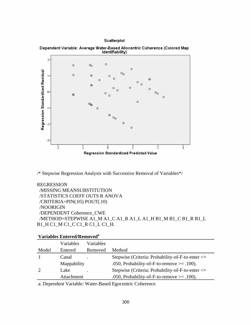
300
/* Stepwise Regression Analysis with Successive Removal of Variables*/
REGRESSION
/MISSING MEANSUBSTITUTION
/STATISTICS COEFF OUTS R ANOVA
/CRITERIA=PIN(.05) POUT(.10)
/NOORIGIN
/DEPENDENT Coherence_CWE
/METHOD=STEPWISE A1_M A1_C A1_R A1_L A1_H B1_M B1_C B1_R B1_L
B1_H C1_M C1_C C1_R C1_L C1_H.
Variables Entered/Removeda
Model
Variables
Entered
Variables
Removed Method
1 Canal
Mappability
. Stepwise (Criteria: Probability-of-F-to-enter <=
.050, Probability-of-F-to-remove >= .100).
2 Lake
Attachment
. Stepwise (Criteria: Probability-of-F-to-enter <=
.050, Probability-of-F-to-remove >= .100).
a. Dependent Variable: Water-Based Egocentric Coherence

301
Model Summary
Model R R Square Adjusted R Square
Std. Error of the
Estimate
1 .438a .192 .177 .67195
2 .505b .255 .226 .65135
a. Predictors: (Constant), Canal Mappability
b. Predictors: (Constant), Canal Mappability, Lake Attachment
ANOVAa
Model
Sum of
Squares df Mean Square F Sig.
1 Regression 5.678 1 5.678 12.576 .001b
Residual 23.931 53 .452
Total 29.609 54
2 Regression 7.547 2 3.774 8.895 .000c
Residual 22.062 52 .424
Total 29.609 54
a. Dependent Variable: Water-Based Egocentric Coherence (Colored Map Procedural
Knowledge)
b. Predictors: (Constant), Canal Mappability
c. Predictors: (Constant), Canal Mappability, Lake Attachment
Coefficientsa
Model
Unstandardized
Coefficients
Standardized
Coefficients
t Sig. B Std. Error Beta
1 (Constant) 1.606 .118 13.646 .000
Canal
Mappability
.119 .034 .438 3.546 .001
2 (Constant) 1.546 .118 13.141 .000
Canal
Mappability
.115 .033 .421 3.511 .001
Lake Attachment .114 .054 .252 2.099 .041
a. Dependent Variable: Water-Based Egocentric Coherence (Colored Map Procedural
Knowledge)

302
Excluded Variablesa
Model Beta In t Sig.
Partial
Correlation
Collinearity
Statistics
Tolerance
1 Waterfront Landmark
Mappability
-.144b -1.153 .254 -.158 .966
River Mappability .000b .001 .999 .000 .961
Lake Mappability .164b 1.330 .189 .181 .987
Harbour Mappability .119b .952 .346 .131 .970
Water Landmark
Identifiability
.066b .521 .604 .072 .962
Canal Identitifiability .002b .011 .991 .002 .671
River Identitifiability .149b 1.199 .236 .164 .983
Lake Identifiability .246b 2.045 .046 .273 .998
Harbour Identifiability .027b .212 .833 .029 .961
Waterfront Landmark
Attachment
-.037b -.298 .767 -.041 .994
Canal Attachment .206b 1.497 .140 .203 .786
River Attachment -.060b -.481 .632 -.067 1.000
Lake Attachment .252b 2.099 .041 .279 .996
Harbour Attachment .006b .047 .962 .007 .992
2 Waterfront Landmark
Mappability
-.090c -.718 .476 -.100 .915
River Mappability .044c .355 .724 .050 .934
Lake Mappability .069c .512 .611 .072 .807
Harbour Mappability .036c .275 .784 .038 .855
Water Landmark
Identifiability
.093c .751 .456 .105 .953
Canal Identitifiability .038c .257 .798 .036 .661
River Identitifiability .183c 1.524 .134 .209 .968
Lake Identifiability .128c .679 .501 .095 .409
Harbour Identifiability -.183c -1.227 .225 -.169 .638
Waterfront Landmark
Attachment
-.020c -.161 .873 -.022 .989
Canal Attachment .243c 1.827 .074 .248 .775
River Attachment -.040c -.329 .743 -.046 .993
Harbour Attachment -.132c -.984 .330 -.137 .796

303
a. Dependent Variable: Water-Based Egocentric Coherence (Colored Map Procedural
Knowledge)
b. Predictors in the Model: (Constant), Canal Mappability
c. Predictors in the Model: (Constant), Canal Mappability, Lake Attachment
/* Stepwise Regression Analysis with Successive Addition of Variables*/
REGRESSION
/MISSING MEANSUBSTITUTION
/STATISTICS COEFF OUTS R ANOVA CHANGE
/CRITERIA=PIN(.05) POUT(.10)
/NOORIGIN
/DEPENDENT Coherence_CWE
/METHOD=STEPWISE A1_C A1_R B1_M
/METHOD=ENTER D1_R
/METHOD=ENTER H5_N
/METHOD=ENTER H2
/METHOD=ENTER AGE
/METHOD=ENTER H13
/METHOD=ENTER H14.
Regression
Variables Entered/Removeda
Model Variables Entered
Variables
Removed Method
1 Canal Mappability . Stepwise (Criteria: Probability-of-
F-to-enter <= .050, Probability-of-
F-to-remove >= .100).
2 Aquaphilia Sensitivity
Baselineb
. Enter
3 Length of Stay Normalizedb . Enter
4 Sexb . Enter
5 Ageb . Enter
6 Incomeb . Enter
7 Educationb . Enter
a. Dependent Variable: Water-Based Egocentric Coherence (Colored Map Procedural
Knowledge)
b. All requested variables entered.

304
Model Summary
Model R
R
Square
Adjusted
R Square
Std. Error
of the
Estimate
Change Statistics
R Square
Change
F
Change df1 df2
Sig. F
Change
1 .438a .192 .177 .67195 .192 12.576 1 53 .001
2 .535b .286 .259 .63761 .094 6.864 1 52 .012
3 .542c .294 .252 .64022 .008 .577 1 51 .451
4 .546d .299 .242 .64449 .005 .326 1 50 .571
5 .573e .328 .260 .63709 .030 2.169 1 49 .147
6 .641f .410 .337 .60310 .082 6.679 1 48 .013
7 .645g .416 .329 .60646 .006 .469 1 47 .497
a. Predictors: (Constant), Canal Mappability
b. Predictors: (Constant), Canal Mappability, Aquaphilia Sensitivity Baseline
c. Predictors: (Constant), Canal Mappability, Aquaphilia Sensitivity Baseline, Length of
Stay Normalized
d. Predictors: (Constant), Canal Mappability, Aquaphilia Sensitivity Baseline, Length of
Stay Normalized, Sex
e. Predictors: (Constant), Canal Mappability, Aquaphilia Sensitivity Baseline, Length of
Stay Normalized, Sex, Age
f. Predictors: (Constant), Canal Mappability, Aquaphilia Sensitivity Baseline, Length of
Stay Normalized, Sex, Age, Income
g. Predictors: (Constant), Canal Mappability, Aquaphilia Sensitivity Baseline, Length of
Stay Normalized, Sex, Age, Income, Education
ANOVAa
Model
Sum of
Squares df Mean Square F Sig.
1 Regression 5.678 1 5.678 12.576 .001b
Residual 23.931 53 .452
Total 29.609 54
2 Regression 8.469 2 4.234 10.416 .000c
Residual 21.140 52 .407
Total 29.609 54
3 Regression 8.705 3 2.902 7.079 .000d
Residual 20.904 51 .410
Total 29.609 54
4 Regression 8.841 4 2.210 5.321 .001e
Residual 20.768 50 .415
Total 29.609 54

305
5 Regression 9.721 5 1.944 4.790 .001f
Residual 19.888 49 .406
Total 29.609 54
6 Regression 12.150 6 2.025 5.567 .000g
Residual 17.459 48 .364
Total 29.609 54
7 Regression 12.323 7 1.760 4.786 .000h
Residual 17.286 47 .368
Total 29.609 54
a. Dependent Variable: Water-Based Egocentric Coherence (Colored Map Procedural
Knowledge)
b. Predictors: (Constant), Canal Mappability
c. Predictors: (Constant), Canal Mappability, Aquaphilia Sensitivity Baseline
d. Predictors: (Constant), Canal Mappability, Aquaphilia Sensitivity Baseline, Length of
Stay Normalized
e. Predictors: (Constant), Canal Mappability, Aquaphilia Sensitivity Baseline, Length of
Stay Normalized, Sex
f. Predictors: (Constant), Canal Mappability, Aquaphilia Sensitivity Baseline, Length of
Stay Normalized, Sex, Age
g. Predictors: (Constant), Canal Mappability, Aquaphilia Sensitivity Baseline, Length of
Stay Normalized, Sex, Age, Income
h. Predictors: (Constant), Canal Mappability, Aquaphilia Sensitivity Baseline, Length of
Stay Normalized, Sex, Age, Income, Education
Coefficientsa
Model
Unstandardized
Coefficients
Standardized
Coefficients
t Sig. B Std. Error Beta
1 (Constant) 1.606 .118 13.646 .000
Canal Mappability .119 .034 .438 3.546 .001
2 (Constant) 2.261 .274 8.261 .000
Canal Mappability .122 .032 .447 3.814 .000
Aquaphilia
Sensitivity Baseline
-.318 .121 -.307 -2.620 .012
3 (Constant) 2.316 .284 8.148 .000
Canal Mappability .123 .032 .450 3.823 .000
Aquaphilia
Sensitivity Baseline
-.325 .122 -.315 -2.664 .010

306
Length of Stay
Normalized
-.047 .062 -.090 -.759 .451
4 (Constant) 2.436 .355 6.869 .000
Canal Mappability .118 .033 .434 3.558 .001
Aquaphilia
Sensitivity Baseline
-.306 .128 -.296 -2.398 .020
Length of Stay
Normalized
-.048 .062 -.091 -.765 .448
Sex -.111 .195 -.072 -.571 .571
5 (Constant) 2.337 .357 6.549 .000
Canal Mappability .126 .033 .465 3.798 .000
Aquaphilia
Sensitivity Baseline
-.281 .127 -.272 -2.209 .032
Length of Stay
Normalized
-.052 .061 -.100 -.849 .400
Sex -.060 .195 -.039 -.305 .761
Age -.001 .000 -.180 -1.473 .147
6 (Constant) 1.994 .363 5.496 .000
Canal Mappability .126 .032 .464 4.004 .000
Aquaphilia
Sensitivity Baseline
-.323 .122 -.313 -2.659 .011
Length of Stay
Normalized
-.073 .059 -.140 -1.245 .219
Sex -.068 .185 -.044 -.366 .716
Age -.001 .000 -.232 -1.969 .055
Income .187 .072 .297 2.584 .013
7 (Constant) 1.772 .489 3.623 .001
Canal Mappability .124 .032 .457 3.905 .000
Aquaphilia
Sensitivity Baseline
-.326 .122 -.315 -2.665 .011
Length of Stay
Normalized
-.068 .060 -.131 -1.146 .258
Sex -.052 .187 -.034 -.278 .782
Age -.001 .000 -.239 -2.011 .050
Income .167 .079 .265 2.113 .040
Education .066 .097 .085 .685 .497
a. Dependent Variable: Water-Based Egocentric Coherence (Colored Map Procedural
Knowledge)

307
Excluded Variablesa
Model Beta In t Sig.
Partial
Correlation
Collinearity
Statistics
Tolerance
1 River Mappability .000b .001 .999 .000 .961
Water Landmark
Identifiability
.066b .521 .604 .072 .962
Aquaphilia Sensitivity
Baseline
-.307b -2.620 .012 -.341 .999
Length of Stay
Normalized
-.063b -.506 .615 -.070 .999
Sex -.150b -1.188 .240 -.163 .952
Age -.233b -1.918 .061 -.257 .982
Income .184b 1.504 .139 .204 .999
Education .137b 1.099 .277 .151 .983
2 River Mappability -.020c -.164 .871 -.023 .957
Water Landmark
Identifiability
.090c .751 .456 .105 .957
Length of Stay
Normalized
-.090c -.759 .451 -.106 .992
Sex -.070c -.560 .578 -.078 .883
Age -.181c -1.526 .133 -.209 .948
Income .240c 2.081 .042 .280 .973
Education .165c 1.406 .166 .193 .975
3 River Mappability -.023d -.190 .850 -.027 .956
Water Landmark
Identifiability
.111d .908 .368 .127 .923
Sex -.072d -.571 .571 -.081 .883
Age -.187d -1.566 .124 -.216 .945
Income .255d 2.201 .032 .297 .957
Education .160d 1.351 .183 .188 .971
4 River Mappability -.015e -.119 .906 -.017 .941
Water Landmark
Identifiability
.120e .966 .339 .137 .913
Age -.180e -1.473 .147 -.206 .915
Income .259e 2.221 .031 .302 .955
Education .156e 1.299 .200 .182 .965
5 River Mappability -.026f -.214 .832 -.031 .937

308
Water Landmark
Identifiability
.096f .771 .444 .111 .894
Income .297f 2.584 .013 .349 .928
Education .185f 1.560 .125 .220 .944
6 River Mappability -.064g -.549 .586 -.080 .923
Water Landmark
Identifiability
.041g .339 .736 .049 .863
Education .085g .685 .497 .099 .806
7 River Mappability -.091h -.751 .457 -.110 .860
Water Landmark
Identifiability
.039h .319 .751 .047 .863
a. Dependent Variable: Water-Based Egocentric Coherence (Colored Map Procedural
Knowledge)
b. Predictors in the Model: (Constant), Canal Mappability
c. Predictors in the Model: (Constant), Canal Mappability, Aquaphilia Sensitivity
Baseline
d. Predictors in the Model: (Constant), Canal Mappability, Aquaphilia Sensitivity
Baseline, Length of Stay Normalized
e. Predictors in the Model: (Constant), Canal Mappability, Aquaphilia Sensitivity
Baseline, Length of Stay Normalized, Sex
f. Predictors in the Model: (Constant), Canal Mappability, Aquaphilia Sensitivity
Baseline, Length of Stay Normalized, Sex, Age
g. Predictors in the Model: (Constant), Canal Mappability, Aquaphilia Sensitivity
Baseline, Length of Stay Normalized, Sex, Age, Income
h. Predictors in the Model: (Constant), Canal Mappability, Aquaphilia Sensitivity
Baseline, Length of Stay Normalized, Sex, Age, Income, Education
/* Final Regression Analysis with IVs identified by Stepwise Regression Analyses.*/
REGRESSION
/MISSING MEANSUBSTITUTION
/STATISTICS COEFF OUTS R ANOVA COLLIN TOL
/CRITERIA=PIN(.05) POUT(.10)
/NOORIGIN
/DEPENDENT Coherence_CWE
/METHOD=ENTER A1_C D1_R
/SCATTERPLOT=(*ZRESID ,*ZPRED)
/SAVE PRED ZPRED COOK LEVER RESID DFBETA SDBETA.

309
Variables Entered/Removeda
Model Variables Entered Variables Removed Method
1 Aquaphilia Sensitivity
Baseline, Canal
Mappability
. Enter
a. Dependent Variable: Water-Based Egocentric Coherence
Model Summaryb
Model R R Square Adjusted R Square
Std. Error of the
Estimate
1 .535a .286 .259 .63761
a. Predictors: (Constant), Aquaphilia Sensitivity Baseline, Canal Mappability
b. Dependent Variable: Water-Based Egocentric Coherence (Colored Map Procedural
Knowledge)
ANOVAa
Model
Sum of
Squares df Mean Square F Sig.
1 Regression 8.469 2 4.234 10.416 .000b
Residual 21.140 52 .407
Total 29.609 54
a. Dependent Variable: Water-Based Egocentric Coherence
b. Predictors: (Constant), Aquaphilia Sensitivity Baseline, Canal Mappability
Coefficientsa
Model
Unstandardized
Coefficients
Standardized
Coefficients
t Sig.
Collinearity
Statistics
B
Std.
Error Beta Tolerance VIF
1 (Constant) 2.261 .274 8.261 .000
Canal
Mappability
.122 .032 .447 3.814 .000 .999 1.001
Aquaphilia
Sensitivity
Baseline
-.318 .121 -.307 -
2.620
.012 .999 1.001
a. Dependent Variable: Water-Based Egocentric Coherence

310
Collinearity Diagnosticsa
Model Dimension Eigenvalue
Condition
Index
Variance Proportions
(Constant)
Canal
Mappability
Aquaphilia
Sensitivity
Baseline
1 1 2.476 1.000 .01 .06 .02
2 .471 2.292 .02 .92 .03
3 .053 6.838 .96 .01 .95
a. Dependent Variable: Water-Based Egocentric Coherence (Colored Map Procedural
Knowledge)
Residuals Statisticsa
Minimum Maximum Mean Std. Deviation N
Predicted Value 1.3080 2.7204 1.8727 .39602 55
Std. Predicted Value -1.426 2.141 .000 1.000 55
Standard Error of
Predicted Value
.086 .233 .144 .037 55
Adjusted Predicted
Value
1.2618 2.7543 1.8738 .39612 55
Residual -1.11218 2.37441 .00000 .62569 55
Std. Residual -1.744 3.724 .000 .981 55
Stud. Residual -1.768 3.783 -.001 1.002 55
Deleted Residual -1.14219 2.44992 -.00108 .65232 55
Stud. Deleted Residual -1.806 4.400 .012 1.055 55
Mahal. Distance .008 6.211 1.964 1.537 55
Cook's Distance .000 .152 .014 .024 55
Centered Leverage
Value
.000 .115 .036 .028 55
a. Dependent Variable: Water-Based Egocentric Coherence

311
REGRESSION
/MISSING LISTWISE
/STATISTICS COEFF OUTS R ANOVA
/CRITERIA=PIN(.05) POUT(.10)
/NOORIGIN
/DEPENDENT D1_R
/METHOD=STEPWISE H5_N AGE H2 H13 H14.
Variables Entered/Removeda
Model
Variables
Entered
Variables
Removed Method
1 Canal
Mappability
. Stepwise (Criteria: Probability-of-F-to-enter
<= .050, Probability-of-F-to-remove >= .100).
2 Length of Stay
Normalized
. Enter
3 Gender . Enter
4 Age . Enter
5 Income . Enter
6 Education . Enter
a. Dependent Variable: Water-Based Egocentric Coherence (Colored Map Procedural
Knowledge)

312
Model Summary
Model R
R
Square
Adjusted
R Square
Std.
Error of
the
Estimate
Change Statistics
R Square
Change
F
Change df1 df2
Sig. F
Change
1 .438a .192 .177 .67195 .192 12.576 1 53 .001
2 .442b .196 .165 .67672 .004 .256 1 52 .615
3 .467c .218 .172 .67385 .022 1.444 1 51 .235
4 .511d .261 .202 .66134 .044 2.947 1 50 .092
5 .569e .324 .254 .63935 .062 4.499 1 49 .039
6 .573f .328 .244 .64386 .004 .316 1 48 .576
a. Predictors: (Constant), Canal Mappability
b. Predictors: (Constant), Canal Mappability, Length of Stay Normalized
c. Predictors: (Constant), Canal Mappability, Length of Stay Normalized, Gender
d. Predictors: (Constant), Canal Mappability, Length of Stay Normalized, Gender, Age
e. Predictors: (Constant), Canal Mappability, Length of Stay Normalized, Gender, Age,
Income
f. Predictors: (Constant), Canal Mappability, Length of Stay Normalized, Gender, Age,
Income, Education

313
ANOVAa
Model
Sum of
Squares df Mean Square F Sig.
1 Regression 5.678 1 5.678 12.576 .001b
Residual 23.931 53 .452
Total 29.609 54
2 Regression 5.796 2 2.898 6.328 .003c
Residual 23.813 52 .458
Total 29.609 54
3 Regression 6.451 3 2.150 4.736 .005d
Residual 23.158 51 .454
Total 29.609 54
4 Regression 7.740 4 1.935 4.424 .004e
Residual 21.869 50 .437
Total 29.609 54
5 Regression 9.579 5 1.916 4.687 .001f
Residual 20.030 49 .409
Total 29.609 54
6 Regression 9.710 6 1.618 3.904 .003g
Residual 19.899 48 .415
Total 29.609 54
a. Dependent Variable: Water-Based Egocentric Coherence (Colored Map Procedural
Knowledge)
b. Predictors: (Constant), Canal Mappability
c. Predictors: (Constant), Canal Mappability, Length of Stay Normalized
d. Predictors: (Constant), Canal Mappability, Length of Stay Normalized, Gender
e. Predictors: (Constant), Canal Mappability, Length of Stay Normalized, Gender, Age
f. Predictors: (Constant), Canal Mappability, Length of Stay Normalized, Gender, Age,
Income
g. Predictors: (Constant), Canal Mappability, Length of Stay Normalized, Gender, Age,
Income, Education

314
Coefficientsa
Model
Unstandardized
Coefficients
Standardized
Coefficients
t Sig. B Std. Error Beta
1 (Constant) 1.606 .118 13.646 .000
Canal Mappability .119 .034 .438 3.546 .001
2 (Constant) 1.634 .130 12.537 .000
Canal Mappability .120 .034 .440 3.536 .001
Length of Stay
Normalized
-.033 .065 -.063 -.506 .615
3 (Constant) 1.974 .311 6.341 .000
Canal Mappability .111 .035 .407 3.203 .002
Length of Stay
Normalized
-.036 .065 -.069 -.556 .580
Gender -.236 .196 -.153 -1.202 .235
4 (Constant) 1.900 .308 6.162 .000
Canal Mappability .121 .034 .446 3.522 .001
Length of Stay
Normalized
-.043 .064 -.082 -.672 .505
Gender -.162 .197 -.105 -.820 .416
Age -.001 .000 -.216 -1.717 .092
5 (Constant) 1.549 .341 4.539 .000
Canal Mappability .121 .033 .443 3.616 .001
Length of Stay
Normalized
-.060 .062 -.114 -.961 .341
Gender -.182 .191 -.118 -.953 .345
Age -.001 .000 -.265 -2.139 .037
Income .161 .076 .256 2.121 .039
6 (Constant) 1.351 .491 2.750 .008
Canal Mappability .119 .034 .437 3.525 .001
Length of Stay
Normalized
-.055 .063 -.106 -.877 .385
Gender -.169 .193 -.110 -.874 .387
Age -.001 .000 -.272 -2.167 .035
Income .143 .083 .228 1.722 .091
Education .058 .103 .074 .562 .576
a. Dependent Variable: Water-Based Egocentric Coherence (Colored Map Procedural
Knowledge)

315
Excluded Variablesa
Model Beta In t Sig.
Partial
Correlation
Collinearity
Statistics
Tolerance
1 River Mappability .000b .001 .999 .000 .961
Water Landmark
Identifiability
.066b .521 .604 .072 .962
Length of Stay
Normalized
-.063b -.506 .615 -.070 .999
Gender -.150b -1.188 .240 -.163 .952
Age -.233b -1.918 .061 -.257 .982
Income .184b 1.504 .139 .204 .999
Education .137b 1.099 .277 .151 .983
2 River Mappability -.002c -.014 .989 -.002 .960
Water Landmark
Identifiability
.080c .619 .539 .086 .931
Gender -.153c -1.202 .235 -.166 .950
Age -.239c -1.949 .057 -.263 .978
Income .193c 1.563 .124 .214 .987
Education .133c 1.056 .296 .146 .978
3 River Mappability .014d .108 .914 .015 .950
Water Landmark
Identifiability
.101d .776 .442 .109 .917
Age -.216d -1.717 .092 -.236 .931
Income .208d 1.695 .096 .233 .979
Education .125d .994 .325 .139 .975
4 River Mappability -.002e -.019 .985 -.003 .945
Water Landmark
Identifiability
.073e .565 .575 .080 .900
Income .256e 2.121 .039 .290 .945
Education .162e 1.311 .196 .184 .951
5 River Mappability -.031f -.254 .801 -.037 .933
Water Landmark
Identifiability
.022f .176 .861 .025 .866
Education .074f .562 .576 .081 .807
6 River Mappability -.052g -.408 .685 -.059 .872
Water Landmark
Identifiability
.020g .159 .875 .023 .865
a. Dependent Variable: Water-Based Egocentric Coherence

316
b. Predictors in the Model: (Constant), Canal Mappability
c. Predictors in the Model: (Constant), Canal Mappability, Length of Stay Normalized
d. Predictors in the Model: (Constant), Canal Mappability, Length of Stay Normalized,
Gender
e. Predictors in the Model: (Constant), Canal Mappability, Length of Stay Normalized,
Gender, Age
f. Predictors in the Model: (Constant), Canal Mappability, Length of Stay Normalized,
Gender, Age, Income
g. Predictors in the Model: (Constant), Canal Mappability, Length of Stay Normalized,
Gender, Age, Income, Education
/* Final Regression Analysis with IVs identified by Previous Stepwise Regression
Analyses.*/
REGRESSION
/MISSING MEANSUBSTITUTION
/STATISTICS COEFF OUTS R ANOVA COLLIN TOL
/CRITERIA=PIN(.05) POUT(.10)
/NOORIGIN
/DEPENDENT Coherence_CWE
/METHOD=ENTER A1_C D1_R
/SCATTERPLOT=(*ZRESID ,*ZPRED)
/SAVE PRED ZPRED COOK LEVER RESID DFBETA SDBETA.
Variables Entered/Removeda
Model Variables Entered Variables Removed Method
1 Aquaphilia Sensitivity
Baseline, Canal
Mappabilityb
. Enter
a. Dependent Variable: Water-Based Egocentric Coherence (Colored Map Procedural
Knowledge)
b. All requested variables entered.
Model Summaryb
Model R R Square Adjusted R Square
Std. Error of the
Estimate
1 .535a .286 .259 .63761
a. Predictors: (Constant), Aquaphilia Sensitivity Baseline, Canal Mappability
b. Dependent Variable: Water-Based Egocentric Coherence

317
ANOVAa
Model
Sum of
Squares df Mean Square F Sig.
1 Regression 8.469 2 4.234 10.416 .000b
Residual 21.140 52 .407
Total 29.609 54
a. Dependent Variable: Water-Based Egocentric Coherence (Colored Map Procedural
Knowledge)
b. Predictors: (Constant), Aquaphilia Sensitivity Baseline, Canal Mappability
Coefficientsa
Model
Unstandardized
Coefficients
Standardized
Coefficients
t Sig.
Collinearity
Statistics
B
Std.
Error Beta Tolerance VIF
1 (Constant) 2.261 .274 8.261 .000
Canal
Mappability
.122 .032 .447 3.814 .000 .999 1.001
Aquaphilia
Sensitivity
Baseline
-.318 .121 -.307 -2.620 .012 .999 1.001
a. Dependent Variable: Water-Based Egocentric Coherence
Collinearity Diagnosticsa
Model Dimension Eigenvalue
Condition
Index
Variance Proportions
(Constant)
Canal
Mappability
Aquaphilia
Sensitivity
Baseline
1 1 2.476 1.000 .01 .06 .02
2 .471 2.292 .02 .92 .03
3 .053 6.838 .96 .01 .95
a. Dependent Variable: Water-Based Egocentric Coherence

318
Residuals Statisticsa
Minimum Maximum Mean Std. Deviation N
Predicted Value 1.3080 2.7204 1.8727 .39602 55
Std. Predicted Value -1.426 2.141 .000 1.000 55
Standard Error of
Predicted Value
.086 .233 .144 .037 55
Adjusted Predicted
Value
1.2618 2.7543 1.8738 .39612 55
Residual -1.11218 2.37441 .00000 .62569 55
Std. Residual -1.744 3.724 .000 .981 55
Stud. Residual -1.768 3.783 -.001 1.002 55
Deleted Residual -1.14219 2.44992 -.00108 .65232 55
Stud. Deleted Residual -1.806 4.400 .012 1.055 55
Mahal. Distance .008 6.211 1.964 1.537 55
Cook's Distance .000 .152 .014 .024 55
Centered Leverage
Value
.000 .115 .036 .028 55
a. Dependent Variable: Water-Based Egocentric Coherence (Colored Map Procedural
Knowledge)

319
/* Final Regression Analysis with IVs identified by Stepwise Regression Analyses.*/
REGRESSION
/MISSING MEANSUBSTITUTION
/STATISTICS COEFF OUTS R ANOVA COLLIN TOL
/CRITERIA=PIN(.05) POUT(.10)
/NOORIGIN
/DEPENDENT Coherence_CWE
/METHOD=ENTER A1_C D1_R AGE H13
/SCATTERPLOT=(*ZRESID ,*ZPRED)
/SAVE PRED ZPRED COOK LEVER RESID DFBETA SDBETA.
Variables Entered/Removeda
Model Variables Entered Variables Removed Method
1 Income, Canal
Mappability, Aquaphilia
Sensitivity Baseline,
Ageb
. Enter
a. Dependent Variable: Water-Based Egocentric Coherence (Colored Map Procedural
Knowledge)
b. All requested variables entered.

320
Model Summaryb
Model R R Square Adjusted R Square
Std. Error of the
Estimate
1 .624a .390 .341 .60113
a. Predictors: (Constant), Income, Canal Mappability, Aquaphilia Sensitivity Baseline,
Age
b. Dependent Variable: Water-Based Egocentric Coherence (Colored Map Procedural
Knowledge)
ANOVAa
Model
Sum of
Squares df Mean Square F Sig.
1 Regression 11.541 4 2.885 7.984 .000b
Residual 18.068 50 .361
Total 29.609 54
a. Dependent Variable: Water-Based Egocentric Coherence (Colored Map Procedural
Knowledge)
b. Predictors: (Constant), Income, Canal Mappability, Aquaphilia Sensitivity Baseline,
Age
Coefficientsa
Model
Unstandardized
Coefficients
Standardized
Coefficients
t Sig.
Collinearity
Statistics
B
Std.
Error Beta Tolerance VIF
1 (Constant) 1.862 .297 6.272 .000
Canal
Mappability
.128 .030 .469 4.207 .000 .982 1.018
Aquaphilia
Sensitivity
Baseline
-.320 .117 -.310 -
2.727
.009 .947 1.056
Age -.001 .000 -.228 -
1.980
.053 .922 1.085
Income .174 .071 .277 2.438 .018 .946 1.057
a. Dependent Variable: Water-Based Egocentric Coherence (Colored Map Procedural
Knowledge)
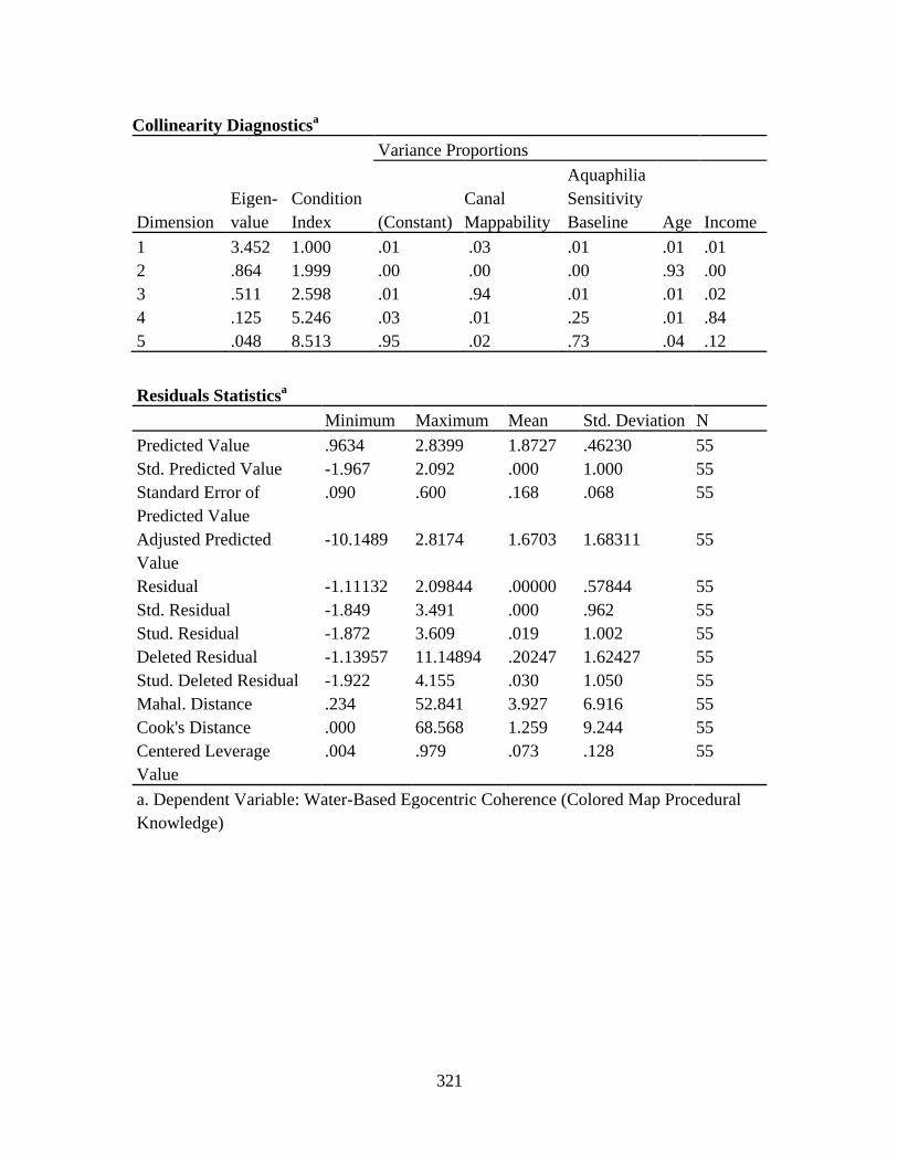
321
Collinearity Diagnosticsa
Dimension
Eigen-
value
Condition
Index
Variance Proportions
(Constant)
Canal
Mappability
Aquaphilia
Sensitivity
Baseline Age
Income
1 3.452 1.000 .01 .03 .01 .01 .01
2 .864 1.999 .00 .00 .00 .93 .00
3 .511 2.598 .01 .94 .01 .01 .02
4 .125 5.246 .03 .01 .25 .01 .84
5 .048 8.513 .95 .02 .73 .04 .12
Residuals Statisticsa
Minimum Maximum Mean Std. Deviation N
Predicted Value .9634 2.8399 1.8727 .46230 55
Std. Predicted Value -1.967 2.092 .000 1.000 55
Standard Error of
Predicted Value
.090 .600 .168 .068 55
Adjusted Predicted
Value
-10.1489 2.8174 1.6703 1.68311 55
Residual -1.11132 2.09844 .00000 .57844 55
Std. Residual -1.849 3.491 .000 .962 55
Stud. Residual -1.872 3.609 .019 1.002 55
Deleted Residual -1.13957 11.14894 .20247 1.62427 55
Stud. Deleted Residual -1.922 4.155 .030 1.050 55
Mahal. Distance .234 52.841 3.927 6.916 55
Cook's Distance .000 68.568 1.259 9.244 55
Centered Leverage
Value
.004 .979 .073 .128 55
a. Dependent Variable: Water-Based Egocentric Coherence (Colored Map Procedural
Knowledge)

322
REGRESSION
/MISSING LISTWISE
/STATISTICS COEFF OUTS R ANOVA
/CRITERIA=PIN(.05) POUT(.10)
/NOORIGIN
/DEPENDENT Coherence_2B
/METHOD=STEPWISE A1_M A1_C A1_R A1_L A1_H B1_M B1_C B1_R B1_L
B1_H C1_M C1_C C1_R C1_L C1_H.
Variables Entered/Removeda
Model Variables Entered Variables Removed Method
1 Water Landmark
Identifiability
. Stepwise (Criteria: Probability-of-
F-to-enter <= .050, Probability-of-
F-to-remove >= .100).
2 River Mappability . Stepwise (Criteria: Probability-of-
F-to-enter <= .050, Probability-of-
F-to-remove >= .100).
3 Canal Mappability . Stepwise (Criteria: Probability-of-
F-to-enter <= .050, Probability-of-
F-to-remove >= .100).
a. Dependent Variable: Coherence Score 2B

323
Model Summary
Model R R Square Adjusted R Square
Std. Error of the
Estimate
1 .365a .133 .117 2.00472
2 .452b .204 .173 1.93941
3 .533c .284 .241 1.85800
a. Predictors: (Constant), Water Landmark Identifiability
b. Predictors: (Constant), Water Landmark Identifiability, River Mappability
c. Predictors: (Constant), Water Landmark Identifiability, River Mappability, Canal
Mappability
ANOVAa
Model
Sum of
Squares df Mean Square F Sig.
1 Regression 32.743 1 32.743 8.147 .006b
Residual 213.002 53 4.019
Total 245.745 54
2 Regression 50.157 2 25.079 6.668 .003c
Residual 195.588 52 3.761
Total 245.745 54
3 Regression 69.685 3 23.228 6.729 .001d
Residual 176.060 51 3.452
Total 245.745 54
a. Dependent Variable: Coherence Score 2B
b. Predictors: (Constant), Water Landmark Identifiability
c. Predictors: (Constant), Water Landmark Identifiability, River Mappability
d. Predictors: (Constant), Water Landmark Identifiability, River Mappability, Canal
Mappability
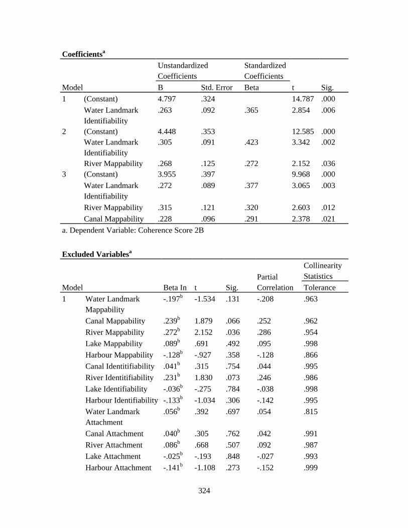
324
Coefficientsa
Model
Unstandardized
Coefficients
Standardized
Coefficients
t Sig. B Std. Error Beta
1 (Constant) 4.797 .324 14.787 .000
Water Landmark
Identifiability
.263 .092 .365 2.854 .006
2 (Constant) 4.448 .353 12.585 .000
Water Landmark
Identifiability
.305 .091 .423 3.342 .002
River Mappability .268 .125 .272 2.152 .036
3 (Constant) 3.955 .397 9.968 .000
Water Landmark
Identifiability
.272 .089 .377 3.065 .003
River Mappability .315 .121 .320 2.603 .012
Canal Mappability .228 .096 .291 2.378 .021
a. Dependent Variable: Coherence Score 2B
Excluded Variablesa
Model Beta In t Sig.
Partial
Correlation
Collinearity
Statistics
Tolerance
1 Water Landmark
Mappability
-.197b -1.534 .131 -.208 .963
Canal Mappability .239b 1.879 .066 .252 .962
River Mappability .272b 2.152 .036 .286 .954
Lake Mappability .089b .691 .492 .095 .998
Harbour Mappability -.128b -.927 .358 -.128 .866
Canal Identitifiability .041b .315 .754 .044 .995
River Identitifiability .231b 1.830 .073 .246 .986
Lake Identifiability -.036b -.275 .784 -.038 .998
Harbour Identifiability -.133b -1.034 .306 -.142 .995
Water Landmark
Attachment
.056b .392 .697 .054 .815
Canal Attachment .040b .305 .762 .042 .991
River Attachment .086b .668 .507 .092 .987
Lake Attachment -.025b -.193 .848 -.027 .993
Harbour Attachment -.141b -1.108 .273 -.152 .999

325
2 Water Landmark
Mappability
-.173c -1.376 .175 -.189 .954
Canal Mappability .291c 2.378 .021 .316 .937
Lake Mappability .102c .818 .417 .114 .996
Harbour Mappability -.070c -.511 .612 -.071 .827
Canal Identitifiability .113c .883 .381 .123 .934
River Identitifiability .183c 1.454 .152 .200 .944
Lake Identifiability .009c .073 .942 .010 .970
Harbour Identifiability -.077c -.601 .551 -.084 .946
Water Landmark
Attachment
.068c .489 .627 .068 .813
Canal Attachment .078c .616 .541 .086 .972
River Attachment -.003c -.022 .982 -.003 .878
Lake Attachment .030c .233 .817 .033 .953
Harbour Attachment -.083c -.650 .518 -.091 .943
3 Water Landmark
Mappability
-.107d -.855 .397 -.120 .894
Lake Mappability .073d .611 .544 .086 .985
Harbour Mappability .031d .222 .826 .031 .745
Canal Identitifiability -.088d -.580 .565 -.082 .613
River Identitifiability .131d 1.054 .297 .147 .908
Lake Identifiability .005d .044 .965 .006 .970
Harbour Identifiability -.010d -.076 .940 -.011 .894
Water Landmark
Attachment
.072d .545 .588 .077 .813
Canal Attachment -.061d -.449 .655 -.063 .782
River Attachment -.024d -.189 .851 -.027 .874
Lake Attachment .014d .116 .908 .016 .950
Harbour Attachment -.046d -.372 .711 -.053 .927
a. Dependent Variable: Coherence Score 2B
b. Predictors in the Model: (Constant), Water Landmark Identifiability
c. Predictors in the Model: (Constant), Water Landmark Identifiability, River
Mappability
d. Predictors in the Model: (Constant), Water Landmark Identifiability, River
Mappability, Canal Mappability

326
REGRESSION
/MISSING LISTWISE
/STATISTICS COEFF OUTS R ANOVA
/CRITERIA=PIN(.05) POUT(.10)
/NOORIGIN
/DEPENDENT Coherence_2B
/METHOD=STEPWISE A1_C A1_R B1_M D1_R.
Variables Entered/Removeda
Model
Variables
Entered
Variables
Removed Method
1 Water
Landmark
Identifiability
. Stepwise (Criteria: Probability-of-F-to-enter <=
.050, Probability-of-F-to-remove >= .100).
2 Aquaphilia
Baseline
. Stepwise (Criteria: Probability-of-F-to-enter <=
.050, Probability-of-F-to-remove >= .100).
3 Canal
Mappability
. Stepwise (Criteria: Probability-of-F-to-enter <=
.050, Probability-of-F-to-remove >= .100).
4 River
Mappability
. Stepwise (Criteria: Probability-of-F-to-enter <=
.050, Probability-of-F-to-remove >= .100).
a. Dependent Variable: Dual-Perspective Coherence (Coding Scheme 2B)
Model Summary
Model R R Square Adjusted R Square
Std. Error of the
Estimate
1 .379a .143 .126 1.99419
2 .533b .285 .255 1.84137
3 .587c .345 .303 1.78040
4 .636d .404 .352 1.71637
a. Predictors: (Constant), Water Landmark Identifiability
b. Predictors: (Constant), Water Landmark Identifiability, Aquaphilia Baseline
c. Predictors: (Constant), Water Landmark Identifiability, Aquaphilia Baseline, Canal
Mappability
d. Predictors: (Constant), Water Landmark Identifiability, Aquaphilia Baseline, Canal
Mappability, River Mappability

327
ANOVAa
Model Sum of Squares df Mean Square F Sig.
1 Regression 32.618 1 32.618 8.202 .006b
Residual 194.863 49 3.977
Total 227.480 50
2 Regression 64.730 2 32.365 9.545 .000c
Residual 162.751 48 3.391
Total 227.480 50
3 Regression 78.498 3 26.166 8.255 .000d
Residual 148.982 47 3.170
Total 227.480 50
4 Regression 91.968 4 22.992 7.805 .000e
Residual 135.513 46 2.946
Total 227.480 50
a. Dependent Variable: Average 8-Stage Coherence (8C)
b. Predictors: (Constant), Water Landmark Identifiability
c. Predictors: (Constant), Water Landmark Identifiability, Aquaphilia Baseline
d. Predictors: (Constant), Water Landmark Identifiability, Aquaphilia Baseline, Canal
Mappability
e. Predictors: (Constant), Water Landmark Identifiability, Aquaphilia Baseline, Canal
Mappability, River Mappability
Excluded Variablesa
Model Beta In t Sig.
Partial
Correlation
Collinearity
Statistics
Tolerance
1 Canal Mappability .246b 1.867 .068 .260 .958
River Mappability .220b 1.661 .103 .233 .962
Aquaphilia Baseline -.377b -3.077 .003 -.406 .993
2 Canal Mappability .251c 2.084 .043 .291 .958
River Mappability .199c 1.625 .111 .231 .959
3 River Mappability .253d 2.138 .038 .301 .928
a. Dependent Variable: Average 8-Stage Coherence (8C)
b. Predictors in the Model: (Constant), Water Landmark Identifiability
c. Predictors in the Model: (Constant), Water Landmark Identifiability, Aquaphilia
Baseline
d. Predictors in the Model: (Constant), Water Landmark Identifiability, Aquaphilia
Baseline, Canal Mappability

328
Coefficientsa
Model
Unstandardized
Coefficients
Standardized
Coefficients
t Sig. B
Std.
Error Beta
1 (Constant) 4.657 .335 13.909 .000
Water Landmark Identifiability .270 .094 .379 2.864 .006
2 (Constant) 6.860 .780 8.798 .000
Water Landmark Identifiability .292 .087 .410 3.344 .002
Aquaphilia Baseline -1.081 .351 -.377 -3.077 .003
3 (Constant) 6.525 .771 8.464 .000
Water Landmark Identifiability .255 .086 .358 2.962 .005
Aquaphilia Baseline -1.090 .340 -.380 -3.211 .002
Canal Mappability .193 .093 .251 2.084 .043
4 (Constant) 6.084 .771 7.890 .000
Water Landmark Identifiability .283 .084 .397 3.365 .002
Aquaphilia Baseline -1.052 .328 -.367 -3.210 .002
Canal Mappability .228 .091 .297 2.512 .016
River Mappability .249 .117 .253 2.138 .038
a. Dependent Variable: Average 8-Stage Coherence (8C)

329
APPENDIX G
LITTLE’S MISSING COMPLETELY AT RANDOM TEST RESULTS
The Composite SEP Model Variables:
Water-Based Familiarity, Water-Based Comfort, Water-Based Place Identity, Water-
Based Place Dependence, Water-Based Place Attachment, Length of Stay
Number of Observed Variables = 6
Number of Missing Data Patterns = 3
Summary of Missing Data Patterns (0 = Missing, 1 = Observed)
Frequency | Pattern | d2j
1 | 1 1 1 0 0 1 | 1.759307
3 | 1 1 1 1 1 0 | 7.449280
26 | 1 1 1 1 1 1 | 0.950342
Sum of the Number of Observed Variables Across Patterns (Sigma psubj) = 15
Little's (1988) Chi-Square Test of MCAR
Chi-Square (d2) = 10.159
df (Sigma psubj - p) = 9
p-value = 0.338

330
SAS SCRIPT
/***********************************************************************
*******************************************/
* *
* This SAS macro implements the chi-square test for a missing completely at random
(MCAR) mechanism, as *
* outlined in Little's (1998) JASA article. Note that the macro requires SAS version 8.2
(or higher) because *
* PROC MI is used to obtain ML estimates of the covariance matrix and mean vector.
* *
* *
/***********************************************************************
*******************************************/;
%macromcartest;
/* SPECIFY FILE PATH FOR THE INPUT DATA */
%letdatafile= 'C:\Users\Owner\Desktop\Data Analysis\SAS\WU.csv';
/* SPECIFY INPUT DATA VARIABLE LIST */
%letvarlist = a1 a2 a3 a4 a5 a6 a7 a8 a9 a10 a11 a12 a13 a14 a15 a16 a17 a18 a19 a20
a21 a22 a23 a24 a25 a26 a27 a28 a29;
/* SPECIFY VARIABLE SET FOR THE MCAR TEST */
%lettestvars = a2 a3 a4 a5 a6 a16;
/* SPECIFY THE MISSING VALUE CODE */
%letmisscode = 9999;
/*******************************/
/* DO NOT ALTER THE CODE BELOW */
/*******************************/
data one;
infile&datafile ;
input&varlist;
%letnumvars = %sysfunc(countw(&testvars));
array m[&numvars] &testvars ;

331
array r[&numvars] r1 - r&numvars ;
doi = 1 to &numvars;
if m[i] = &misscode then m[i] = .;
end;
dropi;
doi = 1 to &numvars;
r[i] = 1;
if m[i] = .then r[i] = 0;
end;
dropi;
proc sort;
by r1-r&numvars;
proc mi data = one nimpute = 0noprint;
var&testvars;
emoutem = emcov;
prociml;
use one;
read all var {&testvars} into y;
read all var {%doi = 1%to&numvars; r&i%end;} into r;
useemcov;
read all var {&testvars} into em;
mu = em[1,];
sigma = em[2:nrow(em),];
/* ASSIGN AN INDEX VARIABLE DENOTING EACH CASE'S PATTERN */
jcol = j(nrow(y), 1 , 1);
doi = 2 to nrow(y);
rdiff = r[i,] - r[i - 1,];
if max(rdiff) = 0& min(rdiff) = 0 then jcol[i,] = jcol[i - 1,];
elsejcol[i,] = jcol[i - 1,] + 1;
end;
/* NUMBER OF DISTINCT MISSING DATA PATTERNS */
j = max(jcol);
/* PUT THE NUMBER OF CASES IN EACH PATTERN IN A COL VECTOR M */

332
/* PUT THE MISSING DATA INDICATORS FOR EACH PATTERN IN A MATRIX
RJ */
m = j(j, 1, 0);
rj = j(j, ncol(r), 0);
doi = 1 to j;
count = 0;
do k = 1 to nrow(y);
ifjcol[k,] = i then do;
count = count + 1;
end;
ifjcol[k,] = i& count = 1 then rj[i,] = r[k,];
m[i,] = count;
end;
end;
/* COMPUTE D^2 STATISTIC FOR EACH J PATTERN */
d2j = j(j, 1, 0);
doi = 1 to j;
/* OBSERVED VALUES FOR PATTERN J */
yj = y[loc(jcol = i),loc(rj[i,] = 1)];
/* VARIABLE MEANS FOR PATTERN J */
ybarobsj = yj[+,]/nrow(yj);
/* D = P X Pj MATRIX OF INDICATORS (SEE P. 1199) */
Dj = j(ncol(y), rj[i,+], 0);
count = 1;
do k = 1 to ncol(rj);
ifrj[i,k] = 1 then do;
Dj[k, count] = 1;
count = count + 1;
end;
end;
/* REDUCE EM ESTIMATES TO CONTAIN OBSERVED ELEMENTS */
muobsj = mu * Dj;
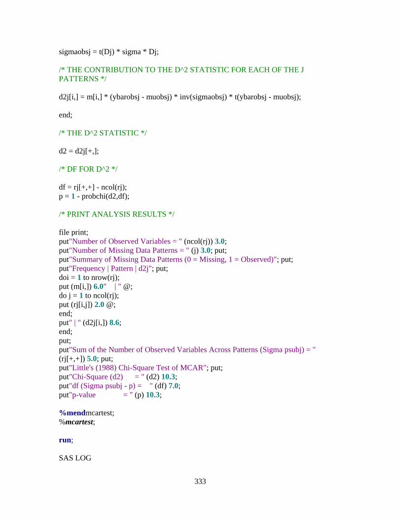
333
sigmaobsj = t(Dj) * sigma * Dj;
/* THE CONTRIBUTION TO THE D^2 STATISTIC FOR EACH OF THE J
PATTERNS */
d2j[i,] = m[i,] * (ybarobsj - muobsj) * inv(sigmaobsj) * t(ybarobsj - muobsj);
end;
/* THE D^2 STATISTIC */
d2 = d2j[+,];
/* DF FOR D^2 */
df = rj[+,+] - ncol(rj);
p = 1 - probchi(d2,df);
/* PRINT ANALYSIS RESULTS */
file print;
put"Number of Observed Variables = " (ncol(rj)) 3.0;
put"Number of Missing Data Patterns = " (j) 3.0; put;
put"Summary of Missing Data Patterns (0 = Missing, 1 = Observed)"; put;
put"Frequency | Pattern | d2j"; put;
doi = 1 to nrow(rj);
put (m[i,]) 6.0" | " @;
do j = 1 to ncol(rj);
put (rj[i,j]) 2.0 @;
end;
put" | " (d2j[i,]) 8.6;
end;
put;
put"Sum of the Number of Observed Variables Across Patterns (Sigma psubj) = "
(rj[+,+]) 5.0; put;
put"Little's (1988) Chi-Square Test of MCAR"; put;
put"Chi-Square (d2) = " (d2) 10.3;
put"df (Sigma psubj - p) = " (df) 7.0;
put"p-value = " (p) 10.3;
%mendmcartest;
%mcartest;
run;
SAS LOG

334
1 The SAS System 14:49 Friday, October 3, 2014
1 ;*';*";*/;quit;run;
2 OPTIONS PAGENO=MIN;
3 %LET _CLIENTTASKLABEL='littles_mcar_test for composite model1';
4 %LET _CLIENTPROJECTPATH='C:\Users\Owner\Desktop\Data
Analysis\SAS\Littles MCAR Test for
4 ! Composite Model.egp';
5 %LET _CLIENTPROJECTNAME='Littles MCAR Test for Composite
Model.egp';
6 %LET _SASPROGRAMFILE=;
7
8 ODS _ALL_ CLOSE;
9 OPTIONS DEV=ACTIVEX;
NOTE: Procedures may not support all options or statements for all devices. For details,
see the
documentation for each procedure.
10 GOPTIONS XPIXELS=0 YPIXELS=0;
11 FILENAME EGSR TEMP;
12 ODS tagsets.sasreport12(ID=EGSR) FILE=EGSR STYLE=Analysis
12 !
STYLESHEET=(URL="file:///C:/Program%20Files/SASHome/x86/BIClientStyles/4.2/
Analysis.css")
12 ! NOGTITLE NOGFOOTNOTE GPATH=&sasworklocation
ENCODING=UTF8 options(rolap="on");
NOTE: Writing TAGSETS.SASREPORT12(EGSR) Body file: EGSR
13
14 GOPTIONS ACCESSIBLE;
15
/***********************************************************************
*****************
15 ! **************************/
16 *
16 ! *
17 * This SAS macro implements the chi-square test for a missing completely at
random
17 ! (MCAR) mechanism, as *
18 * outlined in Little's (1998) JASA article. Note that the macro requires SAS
version
18 ! 8.2 (or higher) because *
19 * PROC MI is used to obtain ML estimates of the covariance matrix and mean
vector.
19 ! * *
20 *
20 ! *

335
21
/***********************************************************************
*****************
21 ! **************************/;
22
23 %macro mcartest;
24
25 /* SPECIFY FILE PATH FOR THE INPUT DATA */
26
27 %let datafile= 'C:\Users\Owner\Desktop\Data Analysis\SAS\WU.csv';
28
29
30 /* SPECIFY INPUT DATA VARIABLE LIST */
31
32 %let varlist = a1 a2 a3 a4 a5 a6 a7 a8 a9 a10 a11 a12 a13 a14 a15 a16 a17 a18
a19 a20 a21
32 ! a22 a23 a24 a25 a26 a27 a28 a29;
33
34 /* SPECIFY VARIABLE SET FOR THE MCAR TEST */
35
36 %let testvars = a2 a3 a4 a5 a6 a16;
37
38 /* SPECIFY THE MISSING VALUE CODE */
39
40 %let misscode = 9999;
2 The SAS System 14:49 Friday, October 3, 2014
41
42 /*******************************/
43 /* DO NOT ALTER THE CODE BELOW */
44 /*******************************/
45
46 data one;
47 infile&datafile ;
48 input &varlist;
49
50 %let numvars = %sysfunc(countw(&testvars));
51
52 array m[&numvars] &testvars ;
53 array r[&numvars] r1 - r&numvars ;
54
55 do i = 1 to &numvars;
56 if m[i] = &misscode then m[i] = .;
57 end;
58 drop i;
59

336
60 do i = 1 to &numvars;
61 r[i] = 1;
62 if m[i] = .then r[i] = 0;
63 end;
64 drop i;
65
66 proc sort;
67 by r1-r&numvars;
68
69 proc mi data = one nimpute = 0 noprint;
70 var&testvars;
71 emoutem = emcov;
72
73 prociml;
74
75 use one;
76 read all var {&testvars} into y;
77 read all var {%do i = 1 %to &numvars; r&i %end;} into r;
78 use emcov;
79 read all var {&testvars} into em;
80
81 mu = em[1,];
82 sigma = em[2:nrow(em),];
83
84 /* ASSIGN AN INDEX VARIABLE DENOTING EACH CASE'S PATTERN */
85
86 jcol = j(nrow(y), 1 , 1);
87
88 do i = 2 to nrow(y);
89 rdiff = r[i,] - r[i - 1,];
90 if max(rdiff) = 0 & min(rdiff) = 0 then jcol[i,] = jcol[i - 1,];
91 else jcol[i,] = jcol[i - 1,] + 1;
92 end;
93
94 /* NUMBER OF DISTINCT MISSING DATA PATTERNS */
3 The SAS System 14:49 Friday, October 3, 2014
95
96 j = max(jcol);
97
98 /* PUT THE NUMBER OF CASES IN EACH PATTERN IN A COL VECTOR
M */
99 /* PUT THE MISSING DATA INDICATORS FOR EACH PATTERN IN A
MATRIX RJ */
100
101 m = j(j, 1, 0);

337
102 rj = j(j, ncol(r), 0);
103
104 do i = 1 to j;
105 count = 0;
106 do k = 1 to nrow(y);
107 if jcol[k,] = i then do;
108 count = count + 1;
109 end;
110 if jcol[k,] = i& count = 1 then rj[i,] = r[k,];
111 m[i,] = count;
112 end;
113 end;
114
115 /* COMPUTE D^2 STATISTIC FOR EACH J PATTERN */
116
117 d2j = j(j, 1, 0);
118
119 do i = 1 to j;
120
121 /* OBSERVED VALUES FOR PATTERN J */
122
123 yj = y[loc(jcol = i),loc(rj[i,] = 1)];
124
125 /* VARIABLE MEANS FOR PATTERN J */
126
127 ybarobsj = yj[+,]/nrow(yj);
128
129 /* D = P X Pj MATRIX OF INDICATORS (SEE P. 1199) */
130
131 Dj = j(ncol(y), rj[i,+], 0);
132
133 count = 1;
134 do k = 1 to ncol(rj);
135 if rj[i,k] = 1 then do;
136 Dj[k, count] = 1;
137 count = count + 1;
138 end;
139 end;
140
141 /* REDUCE EM ESTIMATES TO CONTAIN OBSERVED ELEMENTS */
142
143 muobsj = mu * Dj;
144 sigmaobsj = t(Dj) * sigma * Dj;
145
146 /* THE CONTRIBUTION TO THE D^2 STATISTIC FOR EACH OF THE J
PATTERNS */

338
147
148 d2j[i,] = m[i,] * (ybarobsj - muobsj) * inv(sigmaobsj) * t(ybarobsj - muobsj);
4 The SAS System 14:49 Friday, October 3, 2014
149
150 end;
151
152 /* THE D^2 STATISTIC */
153
154 d2 = d2j[+,];
155
156 /* DF FOR D^2 */
157
158 df = rj[+,+] - ncol(rj);
159 p = 1 - probchi(d2,df);
160
161 /* PRINT ANALYSIS RESULTS */
162
163 file print;
164 put "Number of Observed Variables = " (ncol(rj)) 3.0;
165 put "Number of Missing Data Patterns = " (j) 3.0; put;
166 put "Summary of Missing Data Patterns (0 = Missing, 1 = Observed)"; put;
167 put "Frequency | Pattern | d2j"; put;
168 do i = 1 to nrow(rj);
169 put (m[i,]) 6.0 " | " @;
170 do j = 1 to ncol(rj);
171 put (rj[i,j]) 2.0 @;
172 end;
173 put " | " (d2j[i,]) 8.6;
174 end;
175 put;
176 put "Sum of the Number of Observed Variables Across Patterns (Sigma psubj) =
" (rj[+,+])
176 ! 5.0; put;
177 put "Little's (1988) Chi-Square Test of MCAR"; put;
178 put "Chi-Square (d2) = " (d2) 10.3;
179 put "df (Sigma psubj - p) = " (df) 7.0;
180 put "p-value = " (p) 10.3;
181
182 %mend mcartest;
183 %mcartest;
NOTE: The infile 'C:\Users\Owner\Desktop\Data Analysis\SAS\WU.csv' is:
Filename=C:\Users\Owner\Desktop\Data Analysis\SAS\WU.csv,
RECFM=V,LRECL=256,File Size (bytes)=9026,
Last Modified=03Oct2014:14:48:02,

339
Create Time=02Oct2014:13:41:03
NOTE: 60 records were read from the infile 'C:\Users\Owner\Desktop\Data
Analysis\SAS\WU.csv'.
The minimum record length was 103.
The maximum record length was 193.
NOTE: SAS went to a new line when INPUT statement reached past the end of a line.
NOTE: The data set WORK.ONE has 30 observations and 35 variables.
NOTE: DATA statement used (Total process time):
real time 0.00 seconds
cpu time 0.00 seconds
NOTE: There were 30 observations read from the data set WORK.ONE.
5 The SAS System 14:49 Friday, October 3, 2014
NOTE: The data set WORK.ONE has 30 observations and 35 variables.
NOTE: PROCEDURE SORT used (Total process time):
real time 0.00 seconds
cpu time 0.00 seconds
NOTE: The EM algorithm (MLE) converges in 14 iterations.
NOTE: The data set WORK.EMCOV has 7 observations and 8 variables.
NOTE: PROCEDURE MI used (Total process time):
real time 0.01 seconds
cpu time 0.01 seconds
NOTE: IML Ready
184
185 run;
NOTE: Module MAIN is undefined in IML; cannot be RUN.
186
187
188 GOPTIONS NOACCESSIBLE;
189 %LET _CLIENTTASKLABEL=;
190 %LET _CLIENTPROJECTPATH=;
191 %LET _CLIENTPROJECTNAME=;
192 %LET _SASPROGRAMFILE=;
193
194 ;*';*";*/;quit;
NOTE: Exiting IML.
NOTE: PROCEDURE IML used (Total process time):
real time 0.00 seconds
cpu time 0.01 seconds

340
194 ! run;
195 ODS _ALL_ CLOSE;
196
197
198 QUIT; RUN;
199
The Composite SEP Model Variables (Without Length of Stay):
Water-Based Familiarity, Water-Based Comfort, Water-Based Place Identity, Water-
Based Place Dependence, Water-Based Place Attachment
Number of Observed Variables = 5
Number of Missing Data Patterns = 3
Summary of Missing Data Patterns (0 = Missing, 1 = Observed)
Frequency | Pattern | d2j
1 | 1 1 1 0 0 | 1.414392
5 | 1 1 1 1 0 | 0.933336
24 | 1 1 1 1 1 | 0.290190
Sum of the Number of Observed Variables Across Patterns (Sigma psubj) = 12
Little's (1988) Chi-Square Test of MCAR
Chi-Square (d2) = 2.638
df (Sigma psubj - p) = 7
p-value = 0.916

341
SAS SCRIPT
/***********************************************************************
*******************************************/
* *
* This SAS macro implements the chi-square test for a missing completely at random
(MCAR) mechanism, as *
* outlined in Little's (1998) JASA article. Note that the macro requires SAS version 8.2
(or higher) because *
* PROC MI is used to obtain ML estimates of the covariance matrix and mean vector.
* *
* *
/***********************************************************************
*******************************************/;
%macromcartest;
/* SPECIFY FILE PATH FOR THE INPUT DATA */
%letdatafile= 'C:\Users\Owner\Desktop\Data Analysis\SAS\WU.csv';
/* SPECIFY INPUT DATA VARIABLE LIST */
%letvarlist = a1 a2 a3 a4 a5 a6 a7 a8 a9 a10 a11 a12 a13 a14 a15 a16 a17 a18 a19 a20
a21 a22 a23 a24 a25 a26 a27 a28 a29;
/* SPECIFY VARIABLE SET FOR THE MCAR TEST */
%lettestvars = a2 a3 a4 a6 a7;
/* SPECIFY THE MISSING VALUE CODE */
%letmisscode = 9999;
/*******************************/
/* DO NOT ALTER THE CODE BELOW */
/*******************************/
data one;
infile&datafile ;
input&varlist;
%letnumvars = %sysfunc(countw(&testvars));
array m[&numvars] &testvars ;
array r[&numvars] r1 - r&numvars ;
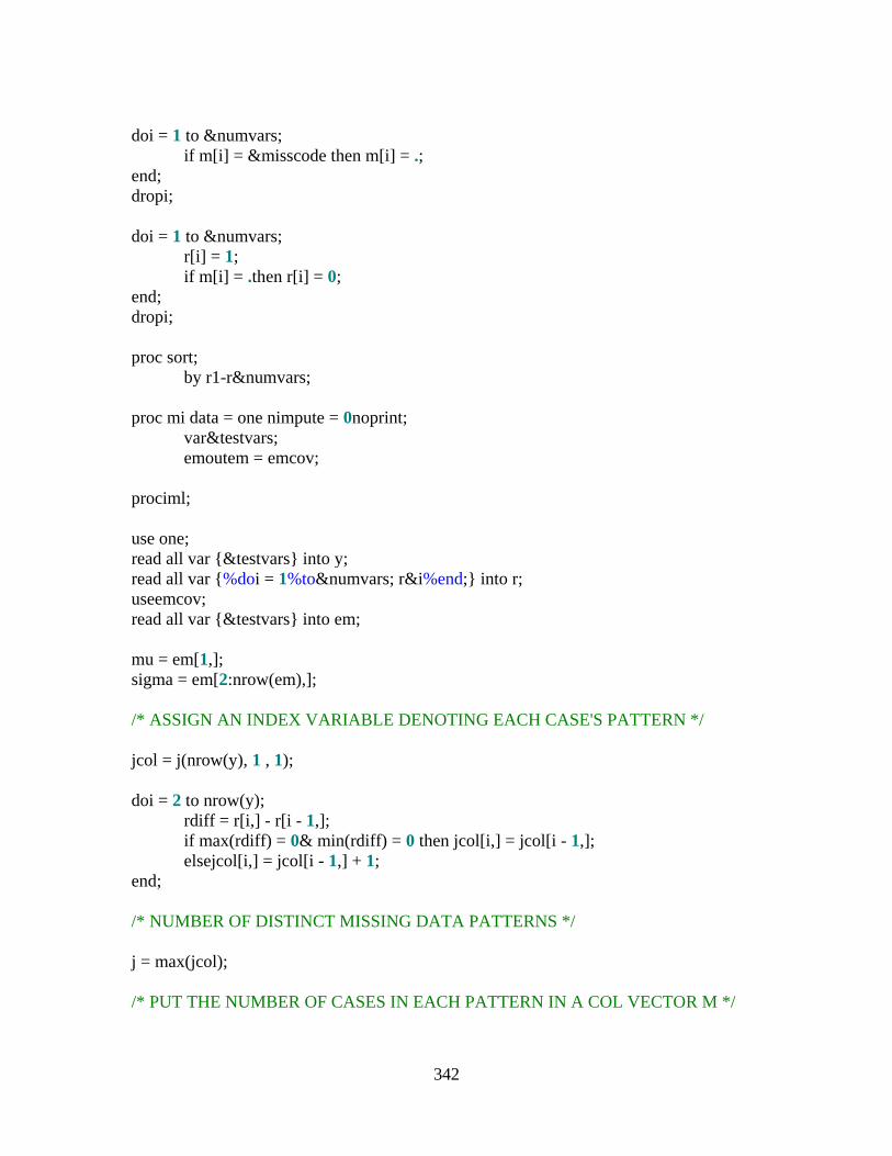
342
doi = 1 to &numvars;
if m[i] = &misscode then m[i] = .;
end;
dropi;
doi = 1 to &numvars;
r[i] = 1;
if m[i] = .then r[i] = 0;
end;
dropi;
proc sort;
by r1-r&numvars;
proc mi data = one nimpute = 0noprint;
var&testvars;
emoutem = emcov;
prociml;
use one;
read all var {&testvars} into y;
read all var {%doi = 1%to&numvars; r&i%end;} into r;
useemcov;
read all var {&testvars} into em;
mu = em[1,];
sigma = em[2:nrow(em),];
/* ASSIGN AN INDEX VARIABLE DENOTING EACH CASE'S PATTERN */
jcol = j(nrow(y), 1 , 1);
doi = 2 to nrow(y);
rdiff = r[i,] - r[i - 1,];
if max(rdiff) = 0& min(rdiff) = 0 then jcol[i,] = jcol[i - 1,];
elsejcol[i,] = jcol[i - 1,] + 1;
end;
/* NUMBER OF DISTINCT MISSING DATA PATTERNS */
j = max(jcol);
/* PUT THE NUMBER OF CASES IN EACH PATTERN IN A COL VECTOR M */

343
/* PUT THE MISSING DATA INDICATORS FOR EACH PATTERN IN A MATRIX
RJ */
m = j(j, 1, 0);
rj = j(j, ncol(r), 0);
doi = 1 to j;
count = 0;
do k = 1 to nrow(y);
ifjcol[k,] = i then do;
count = count + 1;
end;
ifjcol[k,] = i& count = 1 then rj[i,] = r[k,];
m[i,] = count;
end;
end;
/* COMPUTE D^2 STATISTIC FOR EACH J PATTERN */
d2j = j(j, 1, 0);
doi = 1 to j;
/* OBSERVED VALUES FOR PATTERN J */
yj = y[loc(jcol = i),loc(rj[i,] = 1)];
/* VARIABLE MEANS FOR PATTERN J */
ybarobsj = yj[+,]/nrow(yj);
/* D = P X Pj MATRIX OF INDICATORS (SEE P. 1199) */
Dj = j(ncol(y), rj[i,+], 0);
count = 1;
do k = 1 to ncol(rj);
ifrj[i,k] = 1 then do;
Dj[k, count] = 1;
count = count + 1;
end;
end;
/* REDUCE EM ESTIMATES TO CONTAIN OBSERVED ELEMENTS */
muobsj = mu * Dj;

344
sigmaobsj = t(Dj) * sigma * Dj;
/* THE CONTRIBUTION TO THE D^2 STATISTIC FOR EACH OF THE J
PATTERNS */
d2j[i,] = m[i,] * (ybarobsj - muobsj) * inv(sigmaobsj) * t(ybarobsj - muobsj);
end;
/* THE D^2 STATISTIC */
d2 = d2j[+,];
/* DF FOR D^2 */
df = rj[+,+] - ncol(rj);
p = 1 - probchi(d2,df);
/* PRINT ANALYSIS RESULTS */
file print;
put"Number of Observed Variables = " (ncol(rj)) 3.0;
put"Number of Missing Data Patterns = " (j) 3.0; put;
put"Summary of Missing Data Patterns (0 = Missing, 1 = Observed)"; put;
put"Frequency | Pattern | d2j"; put;
doi = 1 to nrow(rj);
put (m[i,]) 6.0" | " @;
do j = 1 to ncol(rj);
put (rj[i,j]) 2.0 @;
end;
put" | " (d2j[i,]) 8.6;
end;
put;
put"Sum of the Number of Observed Variables Across Patterns (Sigma psubj) = "
(rj[+,+]) 5.0; put;
put"Little's (1988) Chi-Square Test of MCAR"; put;
put"Chi-Square (d2) = " (d2) 10.3;
put"df (Sigma psubj - p) = " (df) 7.0;
put"p-value = " (p) 10.3;
%mendmcartest;
%mcartest;
run;
1 ;*';*";*/;quit;run;

345
2 OPTIONS PAGENO=MIN;
3 %LET _CLIENTTASKLABEL='littles_mcar_test without length of stay';
4 %LET _CLIENTPROJECTPATH='';
5 %LET _CLIENTPROJECTNAME='';
6 %LET _SASPROGRAMFILE='C:\Users\Owner\Desktop\Data
Analysis\Final\littles_mcar_test
6 ! without length of stay.sas';
7
8 ODS _ALL_ CLOSE;
9 OPTIONS DEV=ACTIVEX;
NOTE: Procedures may not support all options or statements for all devices. For details,
see the
documentation for each procedure.
10 GOPTIONS XPIXELS=0 YPIXELS=0;
11 FILENAME EGSR TEMP;
12 ODS tagsets.sasreport12(ID=EGSR) FILE=EGSR STYLE=Analysis
12 !
STYLESHEET=(URL="file:///C:/Program%20Files/SASHome/x86/BIClientStyles/4.2/
Analysis.css")
12 ! NOGTITLE NOGFOOTNOTE GPATH=&sasworklocation
ENCODING=UTF8 options(rolap="on");
NOTE: Writing TAGSETS.SASREPORT12(EGSR) Body file: EGSR
13
14 GOPTIONS ACCESSIBLE;
15
/***********************************************************************
*****************
15 ! **************************/
16 *
16 ! *
17 * This SAS macro implements the chi-square test for a missing completely at
random
17 ! (MCAR) mechanism, as *
18 * outlined in Little's (1998) JASA article. Note that the macro requires SAS
version
18 ! 8.2 (or higher) because *
19 * PROC MI is used to obtain ML estimates of the covariance matrix and mean
vector.
19 ! * *
20 *
20 ! *
21
/***********************************************************************
*****************
21 ! **************************/;
22

346
23 %macro mcartest;
24
25 /* SPECIFY FILE PATH FOR THE INPUT DATA */
26
27 %let datafile= 'C:\Users\Owner\Desktop\Data Analysis\SAS\WU.csv';
28
29
30 /* SPECIFY INPUT DATA VARIABLE LIST */
31
32 %let varlist = a1 a2 a3 a4 a5 a6 a7 a8 a9 a10 a11 a12 a13 a14 a15 a16 a17 a18
a19 a20 a21
32 ! a22 a23 a24 a25 a26 a27 a28 a29;
33
34 /* SPECIFY VARIABLE SET FOR THE MCAR TEST */
35
36 %let testvars = a2 a3 a4 a6 a7;
37
38 /* SPECIFY THE MISSING VALUE CODE */
39
2 The SAS System 19:44 Friday, October 3, 2014
40 %let misscode = 9999;
41
42 /*******************************/
43 /* DO NOT ALTER THE CODE BELOW */
44 /*******************************/
45
46 data one;
47 infile&datafile ;
48 input &varlist;
49
50 %let numvars = %sysfunc(countw(&testvars));
51
52 array m[&numvars] &testvars ;
53 array r[&numvars] r1 - r&numvars ;
54
55 do i = 1 to &numvars;
56 if m[i] = &misscode then m[i] = .;
57 end;
58 drop i;
59
60 do i = 1 to &numvars;
61 r[i] = 1;
62 if m[i] = .then r[i] = 0;
63 end;
64 drop i;

347
65
66 proc sort;
67 by r1-r&numvars;
68
69 proc mi data = one nimpute = 0 noprint;
70 var&testvars;
71 emoutem = emcov;
72
73 prociml;
74
75 use one;
76 read all var {&testvars} into y;
77 read all var {%do i = 1 %to &numvars; r&i %end;} into r;
78 use emcov;
79 read all var {&testvars} into em;
80
81 mu = em[1,];
82 sigma = em[2:nrow(em),];
83
84 /* ASSIGN AN INDEX VARIABLE DENOTING EACH CASE'S PATTERN */
85
86 jcol = j(nrow(y), 1 , 1);
87
88 do i = 2 to nrow(y);
89 rdiff = r[i,] - r[i - 1,];
90 if max(rdiff) = 0 & min(rdiff) = 0 then jcol[i,] = jcol[i - 1,];
91 else jcol[i,] = jcol[i - 1,] + 1;
92 end;
93
3 The SAS System 19:44 Friday, October 3, 2014
94 /* NUMBER OF DISTINCT MISSING DATA PATTERNS */
95
96 j = max(jcol);
97
98 /* PUT THE NUMBER OF CASES IN EACH PATTERN IN A COL VECTOR
M */
99 /* PUT THE MISSING DATA INDICATORS FOR EACH PATTERN IN A
MATRIX RJ */
100
101 m = j(j, 1, 0);
102 rj = j(j, ncol(r), 0);
103
104 do i = 1 to j;
105 count = 0;
106 do k = 1 to nrow(y);
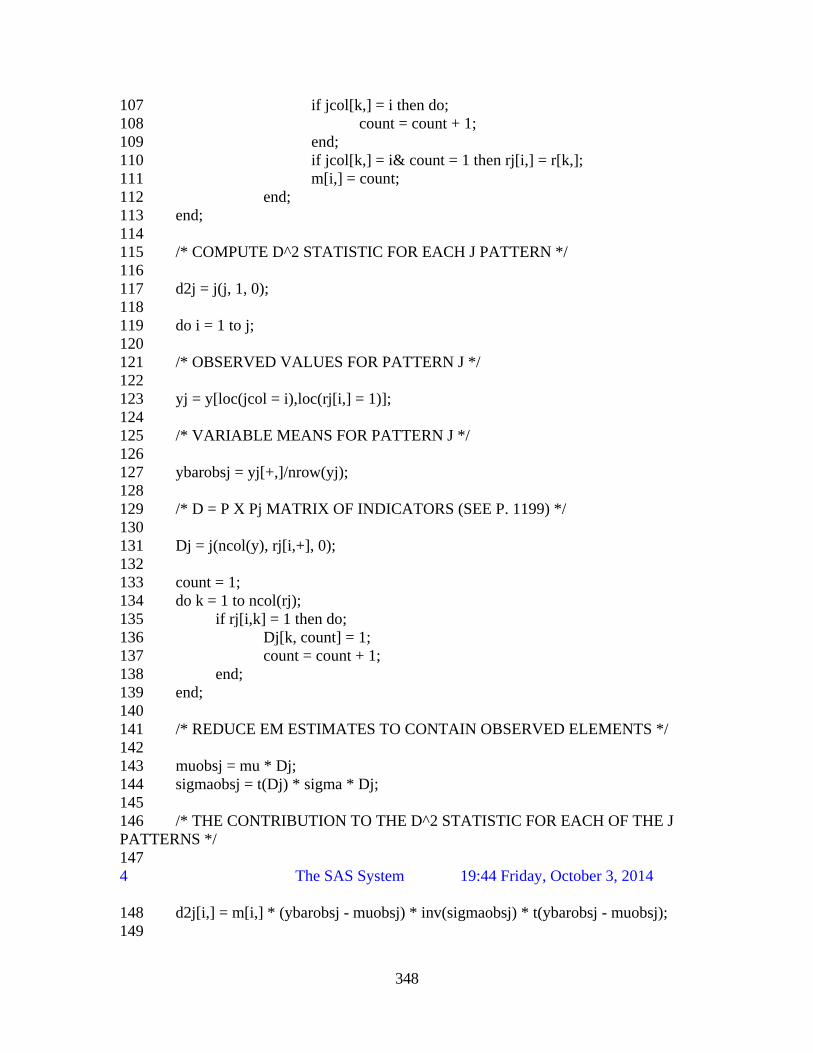
348
107 if jcol[k,] = i then do;
108 count = count + 1;
109 end;
110 if jcol[k,] = i& count = 1 then rj[i,] = r[k,];
111 m[i,] = count;
112 end;
113 end;
114
115 /* COMPUTE D^2 STATISTIC FOR EACH J PATTERN */
116
117 d2j = j(j, 1, 0);
118
119 do i = 1 to j;
120
121 /* OBSERVED VALUES FOR PATTERN J */
122
123 yj = y[loc(jcol = i),loc(rj[i,] = 1)];
124
125 /* VARIABLE MEANS FOR PATTERN J */
126
127 ybarobsj = yj[+,]/nrow(yj);
128
129 /* D = P X Pj MATRIX OF INDICATORS (SEE P. 1199) */
130
131 Dj = j(ncol(y), rj[i,+], 0);
132
133 count = 1;
134 do k = 1 to ncol(rj);
135 if rj[i,k] = 1 then do;
136 Dj[k, count] = 1;
137 count = count + 1;
138 end;
139 end;
140
141 /* REDUCE EM ESTIMATES TO CONTAIN OBSERVED ELEMENTS */
142
143 muobsj = mu * Dj;
144 sigmaobsj = t(Dj) * sigma * Dj;
145
146 /* THE CONTRIBUTION TO THE D^2 STATISTIC FOR EACH OF THE J
PATTERNS */
147
4 The SAS System 19:44 Friday, October 3, 2014
148 d2j[i,] = m[i,] * (ybarobsj - muobsj) * inv(sigmaobsj) * t(ybarobsj - muobsj);
149

349
150 end;
151
152 /* THE D^2 STATISTIC */
153
154 d2 = d2j[+,];
155
156 /* DF FOR D^2 */
157
158 df = rj[+,+] - ncol(rj);
159 p = 1 - probchi(d2,df);
160
161 /* PRINT ANALYSIS RESULTS */
162
163 file print;
164 put "Number of Observed Variables = " (ncol(rj)) 3.0;
165 put "Number of Missing Data Patterns = " (j) 3.0; put;
166 put "Summary of Missing Data Patterns (0 = Missing, 1 = Observed)"; put;
167 put "Frequency | Pattern | d2j"; put;
168 do i = 1 to nrow(rj);
169 put (m[i,]) 6.0 " | " @;
170 do j = 1 to ncol(rj);
171 put (rj[i,j]) 2.0 @;
172 end;
173 put " | " (d2j[i,]) 8.6;
174 end;
175 put;
176 put "Sum of the Number of Observed Variables Across Patterns (Sigma psubj) =
" (rj[+,+])
176 ! 5.0; put;
177 put "Little's (1988) Chi-Square Test of MCAR"; put;
178 put "Chi-Square (d2) = " (d2) 10.3;
179 put "df (Sigma psubj - p) = " (df) 7.0;
180 put "p-value = " (p) 10.3;
181
182 %mend mcartest;
183 %mcartest;
NOTE: The infile 'C:\Users\Owner\Desktop\Data Analysis\SAS\WU.csv' is:
Filename=C:\Users\Owner\Desktop\Data Analysis\SAS\WU.csv,
RECFM=V,LRECL=256,File Size (bytes)=9026,
Last Modified=03Oct2014:14:48:02,
Create Time=02Oct2014:13:41:03
NOTE: 60 records were read from the infile 'C:\Users\Owner\Desktop\Data
Analysis\SAS\WU.csv'.
The minimum record length was 103.

350
The maximum record length was 193.
NOTE: SAS went to a new line when INPUT statement reached past the end of a line.
NOTE: The data set WORK.ONE has 30 observations and 34 variables.
NOTE: DATA statement used (Total process time):
real time 0.00 seconds
cpu time 0.00 seconds
5 The SAS System 19:44 Friday, October 3, 2014
NOTE: There were 30 observations read from the data set WORK.ONE.
NOTE: The data set WORK.ONE has 30 observations and 34 variables.
NOTE: PROCEDURE SORT used (Total process time):
real time 0.01 seconds
cpu time 0.00 seconds
NOTE: The EM algorithm (MLE) converges in 24 iterations.
NOTE: The data set WORK.EMCOV has 6 observations and 7 variables.
NOTE: PROCEDURE MI used (Total process time):
real time 0.01 seconds
cpu time 0.01 seconds
NOTE: IML Ready
184
185 run;
NOTE: Module MAIN is undefined in IML; cannot be RUN.
186
187
188 GOPTIONS NOACCESSIBLE;
189 %LET _CLIENTTASKLABEL=;
190 %LET _CLIENTPROJECTPATH=;
191 %LET _CLIENTPROJECTNAME=;
192 %LET _SASPROGRAMFILE=;
193
194 ;*';*";*/;quit;
NOTE: Exiting IML.
NOTE: PROCEDURE IML used (Total process time):
real time 0.01 seconds
cpu time 0.00 seconds
194 ! run;
195 ODS _ALL_ CLOSE;
196

351
197
198 QUIT; RUN;
199

352
APPENDIX H
NESTED MODEL TESTING RESULTS FROM AMOS
Path Analysis
C:\Users\Owner\Desktop\Dissertation results\Tripartite Comparison.amw
Analysis Summary
Date and Time
Date: Friday, October 03, 2014
Time: 12:25:02 PM
Title
Tripartite comparison: Friday, October 03, 2014 12:25 PM

353
Groups
Group number 1 (Group number 1)
Notes for Group (Group number 1)
The model is recursive.
Sample size = 60
Variable Summary (Tripartite Models)
Your model contains the following variables (Tripartite Models)
Observed, endogenous variables
B1U (water-based place identity or identifiability)
D6 (water-based place dependence or orientation)
C0 (water-based place attachment or allocentric aquaphilia)
D8 (water-based comfort)
H5_C (length of stay normalized)
Observed, exogenous variables
A1U (water-based familiarity)
Unobserved, exogenous variables
e1
e3
e4
e2
e5
Variable counts (Tripartite Models)
Number of variables in your model: 11
Number of observed variables: 6
Number of unobserved variables: 5
Number of exogenous variables: 6
Number of endogenous variables: 5

354
Parameter Summary (Tripartite Models)
Weights Covariances Variances Means Intercepts Total
Fixed 5 0 0 0 0 5
Labeled 9 0 0 0 0 9
Unlabeled 0 0 6 1 5 12
Total 14 0 6 1 5 26
Models
Model 1: Social-Psychological (DI=IA=DA=FI=CD=0) (Model 1: Social-
Psychological (DI=IA=DA=FI=CD=0))
Notes for Model (Model 1: Social-Psychological (DI=IA=DA=FI=CD=0))
Computation of degrees of freedom (Model 1: Social-Psychological
(DI=IA=DA=FI=CD=0))
Number of distinct sample moments: 27
Number of distinct parameters to be estimated: 16
Degrees of freedom (27 - 16): 11
Result (Model 1: Social-Psychological (DI=IA=DA=FI=CD=0))
Minimum was achieved
Chi-square = 52.001
Degrees of freedom = 11
Probability level = .000
Tripartite Models (Tripartite Models - Model 1: Social-Psychological
(DI=IA=DA=FI=CD=0))
Estimates (Tripartite Models - Model 1: Social-Psychological
(DI=IA=DA=FI=CD=0))
Scalar Estimates (Tripartite Models - Model 1: Social-Psychological
(DI=IA=DA=FI=CD=0))
Maximum Likelihood Estimates
Regression Weights: (Tripartite Models - Model 1: Social-Psychological
(DI=IA=DA=FI=CD=0))
Estimate S.E. C.R. P Label
D8 <--- A1U 0.072 0.026 2.709 0.007 FC
D6 <--- D8 0.000
B1U <--- D6 0.000
B1U <--- A1U 0.000

355
Estimate S.E. C.R. P Label
C0 <--- D8 0.137 0.596 0.229 0.819 CA
C0 <--- B1U 0.000
C0 <--- D6 0.000
C0 <--- A1U 0.290 0.123 2.365 0.018 FA
C0 <--- H5_C -0.090 0.306 -0.292 0.770 LA
Standardized Regression Weights: (Tripartite Models - Model 1: Social-Psychological
(DI=IA=DA=FI=CD=0))
Estimate
D8 <--- A1U 0.340
D6 <--- D8 0.000
B1U <--- D6 0.000
B1U <--- A1U 0.000
C0 <--- D8 0.031
C0 <--- B1U 0.000
C0 <--- D6 0.000
C0 <--- A1U 0.311
C0 <--- H5_C -0.038
Means: (Tripartite Models - Model 1: Social-Psychological (DI=IA=DA=FI=CD=0))
Estimate S.E. C.R. P Label
A1U
6.567 0.519 12.658 *** par_6
Intercepts: (Tripartite Models - Model 1: Social-Psychological
(DI=IA=DA=FI=CD=0))
Estimate S.E. C.R. P Label
D8
1.705 0.203 8.396 *** par_7
D6
2.105 0.105 20.009 *** par_8
B1U
4.733 0.534 8.863 *** par_9
H5_C
-0.001 0.212 -0.006 0.995 par_10
C0
1.615 1.346 1.200 0.230 par_5
Variances: (Tripartite Models - Model 1: Social-Psychological
(DI=IA=DA=FI=CD=0))
Estimate S.E. C.R. P Label
A1U
15.879 2.924 5.431 *** par_11
e2
0.622 0.118 5.294 *** par_12
e3
0.620 0.117 5.294 *** par_13
e1
16.829 3.098 5.431 *** par_14
e5
2.441 0.469 5.200 *** par_15
e4
12.375 2.279 5.430 *** par_16

356
Squared Multiple Correlations: (Tripartite Models - Model 1: Social-Psychological
(DI=IA=DA=FI=CD=0))
Estimate
D8
.116
D6
.000
H5_C
.000
B1U
.000
C0
.105
Matrices (Tripartite Models - Model 1: Social-Psychological
(DI=IA=DA=FI=CD=0))
Total Effects (Tripartite Models - Model 1: Social-Psychological
(DI=IA=DA=FI=CD=0))
A1U D8 D6 H5_C B1U
D8 0.072 0.000 0.000 0.000 0.000
D6 0.000 0.000 0.000 0.000 0.000
B1U 0.000 0.000 0.000 0.000 0.000
C0 0.300 0.137 0.000 -0.090 0.000
Standardized Total Effects (Tripartite Models - Model 1: Social-Psychological
(DI=IA=DA=FI=CD=0))
A1U D8 D6 H5_C B1U
D8 0.340 0.000 0.000 0.000 0.000
D6 0.000 0.000 0.000 0.000 0.000
B1U 0.000 0.000 0.000 0.000 0.000
C0 0.321 0.031 0.000 -0.038 0.000
Direct Effects (Tripartite Models - Model 1: Social-Psychological
(DI=IA=DA=FI=CD=0))
A1U D8 D6 H5_C B1U
D8 0.072 0.000 0.000 0.000 0.000
D6 0.000 0.000 0.000 0.000 0.000
B1U 0.000 0.000 0.000 0.000 0.000
C0 0.290 0.137 0.000 -0.090 0.000
Standardized Direct Effects (Tripartite Models - Model 1: Social-Psychological
(DI=IA=DA=FI=CD=0))
A1U D8 D6 H5_C B1U
D8 0.340 0.000 0.000 0.000 0.000
D6 0.000 0.000 0.000 0.000 0.000
B1U 0.000 0.000 0.000 0.000 0.000

357
A1U D8 D6 H5_C B1U
C0 0.311 0.031 0.000 -0.038 0.000
Indirect Effects (Tripartite Models - Model 1: Social-Psychological
(DI=IA=DA=FI=CD=0))
A1U D8 D6 H5_C B1U
D8 0.000 0.000 0.000 0.000 0.000
D6 0.000 0.000 0.000 0.000 0.000
B1U 0.000 0.000 0.000 0.000 0.000
C0 0.010 0.000 0.000 0.000 0.000
Standardized Indirect Effects (Tripartite Models - Model 1: Social-Psychological
(DI=IA=DA=FI=CD=0))
A1U D8 D6 H5_C B1U
D8 0.000 0.000 0.000 0.000 0.000
D6 0.000 0.000 0.000 0.000 0.000
B1U 0.000 0.000 0.000 0.000 0.000
C0 0.010 0.000 0.000 0.000 0.000
Minimization History (Model 1: Social-Psychological (DI=IA=DA=FI=CD=0))
Iteration
Negative
eigen-
values
Condition
# Diameter F NTries Ratio
0 e 0 122.080 9999.000 93.894 0 9999.000
1 e 0 108.718 1.800 77.559 1 0.322
2 e 0 108.894 0.416 56.732 1 1.198
3 e 0 107.552 0.214 52.522 1 1.180
4 e 0 106.413 0.103 52.015 1 1.099
5 e 0 107.043 0.021 52.001 1 1.024
6 e 0 107.117 0.001 52.001 1 1.001
Pairwise Parameter Comparisons (Model 1: Social-Psychological
(DI=IA=DA=FI=CD=0))

358
Variance-covariance Matrix of Estimates (Model 1: Social-Psychological (DI=IA=DA=FI=CD=0))
FC CA FA LA par_5 par_6 par_7 par_8 par_9 par_10 par_11 par_12 par_13 par_14 par_15 par_16
FC 0.001
CA 0.000 0.355
FA 0.000 -0.025 0.015
LA 0.000 0.000 0.000 0.094
par_5 0.000 -0.605 -0.043 0.000 1.811
par_6 0.000 0.000 0.000 0.000 0.000 0.269
par_7 -0.005 0.000 0.000 0.000 0.000 0.000 0.041
par_8 0.000 0.000 0.000 0.000 0.000 0.000 0.000 0.011
par_9 0.000 0.000 0.000 0.000 0.000 0.000 0.000 0.000 0.285
par_10 0.000 0.000 0.000 0.000 0.000 0.000 0.000 0.000 0.000 0.045
par_11 0.000 0.000 0.000 0.000 0.000 0.000 0.000 0.000 0.000 0.000 8.547
par_12 0.000 0.000 0.000 0.000 0.000 0.000 0.000 0.000 0.000 0.000 0.000 0.014
par_13 0.000 0.000 0.000 0.000 0.000 0.000 0.000 0.000 0.000 0.000 0.000 0.000 0.014
par_14 0.000 0.000 0.000 0.000 0.000 0.000 0.000 0.000 0.000 0.000 0.000 0.000 0.000 9.600
par_15 0.000 0.000 0.000 0.000 0.000 0.000 0.000 0.000 0.000 0.000 0.000 0.000 0.000 0.000 0.220
par_16 0.000 -0.003 0.000 0.003 0.005 0.000 0.000 0.000 0.000 0.000 0.000 0.000 0.000 0.000 0.000 5.193

359
Correlations of Estimates (Model 1: Social-Psychological (DI=IA=DA=FI=CD=0))
FC CA FA LA par_5 par_6 par_7 par_8 par_9 par_10 par_11 par_12 par_13 par_14 par_15 par_16
FC 1.000
CA 0.000 1.000
FA -0.001 -0.348 1.000
LA 0.000 0.000 0.000 1.000
par_5 0.001 -0.755 -0.263 0.000 1.000
par_6 0.000 0.000 0.000 0.000 0.000 1.000
par_7 -0.855 0.000 0.001 0.000 -0.001 0.000 1.000
par_8 0.000 0.000 0.000 0.000 0.000 0.000 0.000 1.000
par_9 0.000 0.000 0.000 0.000 0.000 0.000 0.000 0.000 1.000
par_10 0.000 0.000 0.000 0.000 0.001 0.000 0.000 0.000 0.000 1.000
par_11 0.000 0.000 0.000 0.000 0.000 0.000 0.000 0.000 0.000 0.000 1.000
par_12 0.000 0.000 0.000 0.000 0.000 0.000 0.000 0.000 0.000 0.000 0.000 1.000
par_13 0.000 0.000 0.000 0.000 0.000 0.000 0.000 0.000 0.000 0.000 0.000 0.000 1.000
par_14 0.000 0.000 0.000 0.000 0.000 0.000 0.000 0.000 0.000 0.000 0.000 0.000 0.000 1.000
par_15 0.000 0.000 0.000 0.000 0.000 0.000 0.000 0.000 0.000 0.000 0.000 0.000 0.000 0.000 1.000
par_16 0.000 -0.002 0.001 0.005 0.002 0.000 0.000 0.000 0.000 0.000 0.000 0.000 0.000 0.000 0.000 1.000

360
Model 2: Environmental-Psychological (FC=CD=FA=CA=FI=0) (Model 2:
Environmental-Psychological (FC=CD=FA=CA=FI=0))
Notes for Model (Model 2: Environmental-Psychological (FC=CD=FA=CA=FI=0))
Computation of degrees of freedom (Model 2: Environmental-Psychological
(FC=CD=FA=CA=FI=0))
Number of distinct sample moments: 27
Number of distinct parameters to be estimated: 16
Degrees of freedom (27 - 16): 11
Result (Model 2: Environmental-Psychological (FC=CD=FA=CA=FI=0))
Minimum was achieved
Chi-square = 31.276
Degrees of freedom = 11
Probability level = .001
Tripartite Models (Tripartite Models - Model 2: Environmental-Psychological
(FC=CD=FA=CA=FI=0))
Estimates (Tripartite Models - Model 2: Environmental-Psychological
(FC=CD=FA=CA=FI=0))
Scalar Estimates (Tripartite Models - Model 2: Environmental-Psychological
(FC=CD=FA=CA=FI=0))
Maximum Likelihood Estimates
Regression Weights: (Tripartite Models - Model 2: Environmental-Psychological
(FC=CD=FA=CA=FI=0))
Estimate S.E. C.R. P Label
D8 <--- A1U 0.000
D6 <--- D8 0.000
B1U <--- D6 1.903 0.641 2.970 0.003 DI
B1U <--- A1U 0.000
C0 <--- D8 0.000
C0 <--- B1U 0.353 0.101 3.474 *** IA
C0 <--- D6 1.611 0.535 3.013 0.003 DA
C0 <--- A1U 0.000
C0 <--- H5_C -0.024 0.258 -0.094 0.925 LA

361
Standardized Regression Weights: (Tripartite Models - Model 2: Environmental-
Psychological (FC=CD=FA=CA=FI=0))
Estimate
D8 <--- A1U 0.000
D6 <--- D8 0.000
B1U <--- D6 0.366
B1U <--- A1U 0.000
C0 <--- D8 0.000
C0 <--- B1U 0.389
C0 <--- D6 0.342
C0 <--- A1U 0.000
C0 <--- H5_C -0.010
Means: (Tripartite Models - Model 2: Environmental-Psychological
(FC=CD=FA=CA=FI=0))
Estimate S.E. C.R. P Label
A1U
6.567 0.519 12.658 *** par_6
Intercepts: (Tripartite Models - Model 2: Environmental-Psychological
(FC=CD=FA=CA=FI=0))
Estimate S.E. C.R. P Label
D8
2.175 0.112 19.383 *** par_7
D6
2.081 0.105 19.862 *** par_8
B1U
0.772 1.424 0.542 0.588 par_9
H5_C
-0.001 0.212 -0.005 0.996 par_10
C0
-1.205 1.105 -1.091 0.275 par_5
Variances: (Tripartite Models - Model 2: Environmental-Psychological
(FC=CD=FA=CA=FI=0))
Estimate S.E. C.R. P Label
A1U
15.879 2.924 5.431 *** par_11
e2
0.706 0.133 5.294 *** par_12
e3
0.624 0.118 5.302 *** par_13
e1
14.571 2.698 5.401 *** par_14
e5
2.440 0.469 5.200 *** par_15
e4
8.754 1.623 5.395 *** par_16

362
Squared Multiple Correlations: (Tripartite Models - Model 2: Environmental-
Psychological (FC=CD=FA=CA=FI=0))
Estimate
D8
0.000
D6
0.000
H5_C
0.000
B1U
0.134
C0
0.366
Matrices (Tripartite Models - Model 2: Environmental-Psychological
(FC=CD=FA=CA=FI=0))
Total Effects (Tripartite Models - Model 2: Environmental-Psychological
(FC=CD=FA=CA=FI=0))
A1U D8 D6 H5_C B1U
D8 0.000 0.000 0.000 0.000 0.000
D6 0.000 0.000 0.000 0.000 0.000
B1U 0.000 0.000 1.903 0.000 0.000
C0 0.000 0.000 2.282 -0.024 0.353
Standardized Total Effects (Tripartite Models - Model 2: Environmental-
Psychological (FC=CD=FA=CA=FI=0))
A1U D8 D6 H5_C B1U
D8 0.000 0.000 0.000 0.000 0.000
D6 0.000 0.000 0.000 0.000 0.000
B1U 0.000 0.000 0.366 0.000 0.000
C0 0.000 0.000 0.485 -0.010 0.389
Direct Effects (Tripartite Models - Model 2: Environmental-Psychological
(FC=CD=FA=CA=FI=0))
A1U D8 D6 H5_C B1U
D8 0.000 0.000 0.000 0.000 0.000
D6 0.000 0.000 0.000 0.000 0.000
B1U 0.000 0.000 1.903 0.000 0.000
C0 0.000 0.000 1.611 -0.024 0.353

363
Standardized Direct Effects (Tripartite Models - Model 2: Environmental-
Psychological (FC=CD=FA=CA=FI=0))
A1U D8 D6 H5_C B1U
D8 0.000 0.000 0.000 0.000 0.000
D6 0.000 0.000 0.000 0.000 0.000
B1U 0.000 0.000 0.366 0.000 0.000
C0 0.000 0.000 0.342 -0.010 0.389
Indirect Effects (Tripartite Models - Model 2: Environmental-Psychological
(FC=CD=FA=CA=FI=0))
A1U D8 D6 H5_C B1U
D8 0.000 0.000 0.000 0.000 0.000
D6 0.000 0.000 0.000 0.000 0.000
B1U 0.000 0.000 0.000 0.000 0.000
C0 0.000 0.000 0.671 0.000 0.000
Standardized Indirect Effects (Tripartite Models - Model 2: Environmental-
Psychological (FC=CD=FA=CA=FI=0))
A1U D8 D6 H5_C B1U
D8 0.000 0.000 0.000 0.000 0.000
D6 0.000 0.000 0.000 0.000 0.000
B1U 0.000 0.000 0.000 0.000 0.000
C0 0.000 0.000 0.143 0.000 0.000
Minimization History (Model 2: Environmental-Psychological
(FC=CD=FA=CA=FI=0))
Iteration
Negative
eigenvalues
Condition
# Diameter F NTries Ratio
0 e 0 323.527 9999.000 87.995 0 9999.000
1 e 0 233.550 1.612 65.534 3 0.000
2 e 0 141.372 0.917 38.763 1 1.063
3 e 0 117.333 0.180 32.590 1 1.215
4 e 0 108.712 0.092 31.372 1 1.154
5 e 0 99.809 0.032 31.277 1 1.063
6 e 0 100.466 0.004 31.276 1 1.007
7 e 0 100.547 0.000 31.276 1 1.000

364
Pairwise Parameter Comparisons (Model 2: Environmental-Psychological (FC=CD=FA=CA=FI=0))
Variance-covariance Matrix of Estimates (Model 2: Environmental-Psychological (FC=CD=FA=CA=FI=0))
DI IA DA LA par_5 par_6 par_7 par_8 par_9 par_10 par_11 par_12 par_13 par_14 par_15 par_16
DI 0.410
IA -0.001 0.010
DA 0.001 -0.020 0.286
LA 0.000 0.000 0.000 0.067
par_5 0.003 -0.007 -0.500 0.000 1.222
par_6 0.000 0.000 0.000 0.000 0.000 0.269
par_7 0.000 0.000 0.000 0.000 0.000 0.000 0.013
par_8 0.000 0.000 0.000 0.000 -0.001 0.000 0.000 0.011
par_9 -0.854 0.002 -0.001 0.000 -0.004 0.000 0.000 -0.001 2.027
par_10 0.000 0.000 0.000 0.000 0.000 0.000 0.000 0.000 0.000 0.045
par_11 0.000 0.000 0.000 0.000 0.000 0.000 0.000 0.000 0.000 0.000 8.547
par_12 0.000 0.000 0.000 0.000 0.000 0.000 0.000 0.000 0.000 0.000 0.000 0.018
par_13 0.000 0.000 0.000 0.000 0.001 0.000 0.000 0.000 0.001 0.000 0.000 0.000 0.014
par_14 -0.033 0.002 -0.001 0.000 -0.009 0.000 0.000 0.000 0.068 0.000 0.000 0.000 -0.001 7.280
par_15 0.000 0.000 0.000 0.000 0.000 0.000 0.000 0.000 0.000 0.000 0.000 0.000 0.000 0.000 0.220
par_16 0.003 0.001 -0.019 0.001 0.033 0.000 0.000 0.000 -0.006 0.000 0.000 0.000 -0.001 -0.004 0.000 2.633

365
Correlations of Estimates (Model 2: Environmental-Psychological (FC=CD=FA=CA=FI=0))
DI IA DA LA par_5 par_6 par_7 par_8 par_9 par_10 par_11 par_12 par_13 par_14 par_15 par_16
DI 1.000
IA -0.013 1.000
DA 0.002 -0.371 1.000
LA 0.000 0.000 0.000 1.000
par_5 0.004 -0.061 -0.845 0.000 1.000
par_6 0.000 0.000 0.000 0.000 0.000 1.000
par_7 0.000 0.000 0.000 0.000 0.000 0.000 1.000
par_8 0.000 0.000 0.000 0.000 -0.006 0.000 0.000 1.000
par_9 -0.937 0.012 -0.002 0.000 -0.003 0.000 0.000 -0.005 1.000
par_10 0.000 0.000 0.000 0.000 0.000 0.000 0.000 0.000 0.000 1.000
par_11 0.000 0.000 0.000 0.000 0.000 0.000 0.000 0.000 0.000 0.000 1.000
par_12 0.000 0.000 0.000 0.000 0.000 0.000 0.000 0.000 0.000 0.000 0.000 1.000
par_13 -0.005 -0.007 -0.003 0.000 0.006 0.000 0.000 0.000 0.005 0.000 0.000 0.000 1.000
par_14 -0.019 0.008 0.000 0.000 -0.003 0.000 0.000 0.000 0.018 0.000 0.000 0.000 -0.004 1.000
par_15 0.000 0.000 0.000 0.000 0.000 0.000 0.000 0.000 0.000 0.000 0.000 0.000 0.000 0.000 1.000
par_16 0.003 0.008 -0.022 0.002 0.018 0.000 0.000 0.000 -0.003 0.000 0.000 0.000 -0.005 -0.001 0.000 1.000

366
Model 3: Composite (FA=CA=0) (Model 3: Composite (FA=CA=0))
Notes for Model (Model 3: Composite (FA=CA=0))
Computation of degrees of freedom (Model 3: Composite (FA=CA=0))
Number of distinct sample moments: 27
Number of distinct parameters to be estimated: 19
Degrees of freedom (27 - 19): 8
Result (Model 3: Composite (FA=CA=0))
Minimum was achieved
Chi-square = 3.589
Degrees of freedom = 8
Probability level = .892
Tripartite Models (Tripartite Models - Model 3: Composite (FA=CA=0))
Estimates (Tripartite Models - Model 3: Composite (FA=CA=0))
Scalar Estimates (Tripartite Models - Model 3: Composite (FA=CA=0))
Maximum Likelihood Estimates
Regression Weights: (Tripartite Models - Model 3: Composite (FA=CA=0))
Estimate S.E. C.R. P Label
D8 <--- A1U 0.071 0.026 2.691 0.007 FC
D6 <--- D8 0.346 0.117 2.963 0.003 CD
B1U <--- D6 1.357 0.582 2.333 0.020 DI
B1U <--- A1U 0.432 0.113 3.810 *** FI
C0 <--- D8 0.000
C0 <--- B1U 0.353 0.101 3.498 *** IA
C0 <--- D6 1.606 0.525 3.061 0.002 DA
C0 <--- A1U 0.000
C0 <--- H5_C -0.024 0.258 -0.092 0.927 LA

367
Standardized Regression Weights: (Tripartite Models - Model 3: Composite
(FA=CA=0))
Estimate
D8 <--- A1U 0.338
D6 <--- D8 0.368
B1U <--- D6 0.265
B1U <--- A1U 0.425
C0 <--- D8 0.000
C0 <--- B1U 0.388
C0 <--- D6 0.344
C0 <--- A1U 0.000
C0 <--- H5_C -0.010
Means: (Tripartite Models - Model 3: Composite (FA=CA=0))
Estimate S.E. C.R. P Label
A1U 6.567 0.519 12.658 *** par_9
Intercepts: (Tripartite Models - Model 3: Composite (FA=CA=0))
Estimate S.E. C.R. P Label
D8 1.702 0.203 8.379 *** par_10
D6 1.331 0.272 4.901 *** par_11
B1U -0.929 1.412 -0.658 0.510 par_12
H5_C -0.001 0.212 -0.005 0.996 par_13
C0 -1.200 1.111 -1.080 0.280 par_8
Variances: (Tripartite Models - Model 3: Composite (FA=CA=0))
Estimate S.E. C.R. P Label
A1U 15.879 2.924 5.431 *** par_14
e2 0.623 0.118 5.294 *** par_15
e3 0.539 0.102 5.299 *** par_16
e1 11.802 2.181 5.411 *** par_17
e5 2.440 0.469 5.200 *** par_18
e4 8.761 1.624 5.394 *** par_19

368
Squared Multiple Correlations: (Tripartite Models - Model 3: Composite
(FA=CA=0))
Estimate
D8 0.114
D6 0.135
H5_C 0.000
B1U 0.279
C0 0.354
Matrices (Tripartite Models - Model 3: Composite (FA=CA=0))
Total Effects (Tripartite Models - Model 3: Composite (FA=CA=0))
A1U D8 D6 H5_C B1U
D8 0.071 0.000 0.000 0.000 0.000
D6 0.025 0.346 0.000 0.000 0.000
B1U 0.465 0.470 1.357 0.000 0.000
C0 0.204 0.722 2.086 -0.024 0.353
Standardized Total Effects (Tripartite Models - Model 3: Composite (FA=CA=0))
A1U D8 D6 H5_C B1U
D8 0.338 0.000 0.000 0.000 0.000
D6 0.124 0.368 0.000 0.000 0.000
B1U 0.458 0.097 0.265 0.000 0.000
C0 0.221 0.164 0.447 -0.010 0.388
Direct Effects (Tripartite Models - Model 3: Composite (FA=CA=0))
A1U D8 D6 H5_C B1U
D8 0.071 0.000 0.000 0.000 0.000
D6 0.000 0.346 0.000 0.000 0.000
B1U 0.432 0.000 1.357 0.000 0.000
C0 0.000 0.000 1.606 -0.024 0.353
Standardized Direct Effects (Tripartite Models - Model 3: Composite (FA=CA=0))
A1U D8 D6 H5_C B1U
D8 0.338 0.000 0.000 0.000 0.000
D6 0.000 0.368 0.000 0.000 0.000
B1U 0.425 0.000 0.265 0.000 0.000
C0 0.000 0.000 0.344 -0.010 0.388

369
Indirect Effects (Tripartite Models - Model 3: Composite (FA=CA=0))
A1U D8 D6 H5_C B1U
D8 0.000 0.000 0.000 0.000 0.000
D6 0.025 0.000 0.000 0.000 0.000
B1U 0.033 0.470 0.000 0.000 0.000
C0 0.204 0.722 0.479 0.000 0.000
Standardized Indirect Effects (Tripartite Models - Model 3: Composite (FA=CA=0))
A1U D8 D6 H5_C B1U
D8 0.000 0.000 0.000 0.000 0.000
D6 0.124 0.000 0.000 0.000 0.000
B1U 0.033 0.097 0.000 0.000 0.000
C0 0.221 0.164 0.103 0.000 0.000
Minimization History (Model 3: Composite (FA=CA=0))
Iteration
Negative
eigenvalues
Condition
# Diameter F NTries Ratio
0 e 0 405.617 9999.000 88.734 0 9999.000
1 e 0 157.121 1.854 43.802 3 .000
2 e 0 126.051 .921 10.855 1 1.034
3 e 0 104.748 .195 4.714 1 1.199
4 e 0 91.224 .089 3.661 1 1.144
5 e 0 93.426 .028 3.589 1 1.056
6 e 0 94.272 .003 3.589 1 1.006
7 e 0 94.597 .000 3.589 1 1.000

370
Pairwise Parameter Comparisons (Model 3: Composite (FA=CA=0))
Variance-covariance Matrix of Estimates (Model 3: Composite (FA=CA=0))
DI FC FI CD IA DA LA par_8 par_9 par_10 par_11 par_12 par_13 par_14 par_15 par_16 par_17 par_18 par_19
DI 0.338
FC 0.000 0.001
FI -0.008 0.000 0.013
CD 0.000 0.000 0.000 0.014
IA -0.001 0.000 0.000 0.000 0.010
DA 0.000 0.000 0.000 0.000 -0.017 0.275
LA 0.000 0.000 0.000 0.000 0.000 0.000 0.067
par_8 0.003 0.000 0.000 0.000 -0.013 -0.493 0.000 1.235
par_9 0.000 0.000 0.000 0.000 0.000 0.000 0.000 0.000 0.269
par_10 0.000 -0.005 0.000 0.000 0.000 0.000 0.000 0.000 0.000 0.041
par_11 0.000 0.000 0.000 -0.030 0.000 0.000 0.000 -0.002 0.000 0.000 0.074
par_12 -0.650 0.000 -0.067 0.001 0.001 -0.001 0.000 -0.004 0.000 -0.001 -0.002 1.994
par_13 0.000 0.000 0.000 0.000 0.000 0.000 0.000 0.000 0.000 0.000 0.000 0.000 0.045
par_14 0.000 0.000 0.000 0.000 0.000 0.000 0.000 0.000 0.000 0.000 0.000 0.000 0.000 8.547
par_15 0.000 0.000 0.000 0.000 0.000 0.000 0.000 0.000 0.000 0.000 0.000 0.000 0.000 0.000 0.014
par_16 0.000 0.000 0.000 0.000 0.000 0.000 0.000 0.001 0.000 0.000 0.000 0.000 0.000 0.000 0.000 0.010
par_17 -0.021 0.000 0.001 0.000 0.001 0.000 0.000 -0.006 0.000 0.000 0.001 0.040 0.000 0.000 0.000 -0.001 4.758
par_18 0.000 0.000 0.000 0.000 0.000 0.000 0.000 0.000 0.000 0.000 0.000 0.000 0.000 0.000 0.000 0.000 0.000 0.220
par_19 0.002 0.000 0.000 0.000 0.001 -0.018 0.001 0.033 0.000 0.000 0.001 -0.005 0.000 0.000 0.000 -0.001 -0.002 0.000 2.638
Correlations of Estimates (Model 3: Composite (FA=CA=0))
DI FC FI CD IA DA LA par_8 par_9 par_10 par_11 par_12 par_13 par_14 par_15 par_16 par_17 par_18 par_19
DI 1.000
FC 0.000 1.000
FI -0.126 -0.004 1.000
CD -0.002 -0.001 -0.004 1.000
IA -0.013 -0.003 0.004 -0.005 1.000
DA 0.001 0.000 0.000 -0.001 -0.322 1.000
LA 0.000 0.000 0.000 0.000 0.000 0.000 1.000
par_8 0.004 0.001 -0.001 0.003 -0.113 -0.845 0.000 1.000
par_9 0.000 0.000 0.000 0.000 0.000 0.000 0.000 0.000 1.000
par_10 0.000 -0.855 0.004 0.001 0.002 0.000 0.000 -0.002 0.000 1.000
par_11 0.001 0.001 0.003 -0.933 0.004 0.001 0.000 -0.005 0.000 -0.002 1.000
par_12 -0.791 0.002 -.0419 0.003 0.009 -0.001 0.000 -0.002 0.000 -0.003 -0.004 1.000
par_13 0.000 0.000 .0000 0.000 0.000 0.000 0.000 0.000 0.000 0.000 0.000 0.000 1.000
par_14 0.000 0.000 .0000 0.000 0.000 0.000 0.000 0.000 0.000 0.000 0.000 0.000 0.000 1.000
par_15 0.000 0.000 .0000 0.000 -0.001 0.000 0.000 0.001 0.000 0.000 0.000 0.000 0.000 0.000 1.000
par_16 -0.003 0.000 .0000 -0.001 -0.004 -0.003 0.000 0.005 0.000 0.000 0.001 0.003 0.000 0.000 0.000 1.000
par_17 -0.016 0.000 .0002 -0.001 0.006 0.000 0.000 -0.002 0.000 0.000 0.001 0.013 0.000 0.000 0.000 -0.003 1.000
par_18 0.000 0.000 .0000 0.000 0.000 0.000 0.000 0.000 0.000 0.000 0.000 0.000 0.000 0.000 0.000 0.000 0.000 1.000
par_19 0.002 0.000 .0000 -0.002 0.007 -0.022 0.001 0.018 0.000 0.000 0.002 -0.002 0.000 0.000 -0.001 -0.005 -0.001 0.000 1.000

371
Model 4: Composite without controlling Length of Stay (FA=CA=LA=0) (Model 4:
Composite without controlling Length of Stay (FA=CA=LA=0))
Notes for Model (Model 4: Composite without controlling Length of Stay
(FA=CA=LA=0))
Computation of degrees of freedom (Model 4: Composite without controlling Length
of Stay (FA=CA=LA=0))
Number of distinct sample moments: 27
Number of distinct parameters to be estimated: 18
Degrees of freedom (27 - 18): 9
Result (Model 4: Composite without controlling Length of Stay (FA=CA=LA=0))
Minimum was achieved
Chi-square = 3.596
Degrees of freedom = 9
Probability level = .936
Tripartite Models (Tripartite Models - Model 4: Composite without controlling
Length of Stay (FA=CA=LA=0))
Estimates (Tripartite Models - Model 4: Composite without controlling Length of
Stay (FA=CA=LA=0))
Scalar Estimates (Tripartite Models - Model 4: Composite without controlling Length
of Stay (FA=CA=LA=0))
Maximum Likelihood Estimates
Regression Weights: (Tripartite Models - Model 4: Composite without controlling
Length of Stay (FA=CA=LA=0))
Estimate S.E. C.R. P Label
D8 <--- A1U 0.071 0.026 2.691 0.007 FC
D6 <--- D8 0.346 0.117 2.963 0.003 CD
B1U <--- D6 1.358 0.582 2.333 0.020 DI
B1U <--- A1U 0.432 0.113 3.810 *** FI
C0 <--- D8 0.000
C0 <--- B1U 0.354 0.101 3.502 *** IA
C0 <--- D6 1.605 0.525 3.057 0.002 DA
C0 <--- A1U 0.000
C0 <--- H5_C 0.000

372
Standardized Regression Weights: (Tripartite Models - Model 4: Composite without
controlling Length of Stay (FA=CA=LA=0))
Estimate
D8 <--- A1U .338
D6 <--- D8 .368
B1U <--- D6 .265
B1U <--- A1U .425
C0 <--- D8 .000
C0 <--- B1U .388
C0 <--- D6 .344
C0 <--- A1U .000
C0 <--- H5_C .000
Means: (Tripartite Models - Model 4: Composite without controlling Length of Stay
(FA=CA=LA=0))
Estimate S.E. C.R. P Label
A1U
6.567 .519 12.658 *** par_8
Intercepts: (Tripartite Models - Model 4: Composite without controlling Length of
Stay (FA=CA=LA=0))
Estimate S.E. C.R. P Label
D8 1.702 0.203 8.379 *** par_9
D6 1.331 0.272 4.901 *** par_10
B1U -0.930 1.412 -0.658 0.510 par_11
H5_C 0.000 0.212 0.000 1.000 par_12
C0 -1.198 1.112 -1.078 0.281 par_7
Variances: (Tripartite Models - Model 4: Composite without controlling Length of
Stay (FA=CA=LA=0))
Estimate S.E. C.R. P Label
A1U 15.879 2.924 5.431 *** par_13
e2 0.623 0.118 5.294 *** par_14
e3 0.539 0.102 5.299 *** par_15
e1 11.802 2.181 5.411 *** par_16
e5 2.440 0.469 5.200 *** par_17
e4 8.762 1.624 5.394 *** par_18

373
Squared Multiple Correlations: (Tripartite Models - Model 4: Composite without
controlling Length of Stay (FA=CA=LA=0))
Estimate
D8 0.114
D6 0.135
H5_C 0.000
B1U 0.279
C0 0.354
Matrices (Tripartite Models - Model 4: Composite without controlling Length of Stay
(FA=CA=LA=0))
Total Effects (Tripartite Models - Model 4: Composite without controlling Length of
Stay (FA=CA=LA=0))
A1U D8 D6 H5_C B1U
D8 0.071 0.000 0.000 0.000 0.000
D6 0.025 0.346 0.000 0.000 0.000
B1U 0.465 0.470 1.358 0.000 0.000
C0 0.204 0.722 2.085 0.000 0.354
Standardized Total Effects (Tripartite Models - Model 4: Composite without
controlling Length of Stay (FA=CA=LA=0))
A1U D8 D6 H5_C B1U
D8 0.338 0.000 0.000 0.000 0.000
D6 0.124 0.368 0.000 0.000 0.000
B1U 0.458 0.097 0.265 0.000 0.000
C0 0.221 0.164 0.447 0.000 0.388
Direct Effects (Tripartite Models - Model 4: Composite without controlling Length of
Stay (FA=CA=LA=0))
A1U D8 D6 H5_C B1U
D8 0.071 0.000 0.000 0.000 0.000
D6 0.000 0.346 0.000 0.000 0.000
B1U 0.432 0.000 1.358 0.000 0.000
C0 0.000 0.000 1.605 0.000 0.354
Standardized Direct Effects (Tripartite Models - Model 4: Composite without
controlling Length of Stay (FA=CA=LA=0))
A1U D8 D6 H5_C B1U
D8 0.338 0.000 0.000 0.000 0.000
D6 0.000 0.368 0.000 0.000 0.000
B1U 0.425 0.000 0.265 0.000 0.000

374
A1U D8 D6 H5_C B1U
C0 0.000 0.000 0.344 0.000 0.388
Indirect Effects (Tripartite Models - Model 4: Composite without controlling Length
of Stay (FA=CA=LA=0))
A1U D8 D6 H5_C B1U
D8 0.000 0.000 0.000 0.000 0.000
D6 0.025 0.000 0.000 0.000 0.000
B1U 0.033 0.470 0.000 0.000 0.000
C0 0.204 0.722 0.480 0.000 0.000
Standardized Indirect Effects (Tripartite Models - Model 4: Composite without
controlling Length of Stay (FA=CA=LA=0))
A1U D8 D6 H5_C B1U
D8 0.000 0.000 0.000 0.000 0.000
D6 0.124 0.000 0.000 0.000 0.000
B1U 0.033 0.097 0.000 0.000 0.000
C0 0.221 0.164 0.103 0.000 0.000
Minimization History (Model 4: Composite without controlling Length of Stay
(FA=CA=LA=0))
Iteration
Negative
eigenvalues
Condition
# Diameter F NTries Ratio
0 e 0 400.458 9999.000 87.873 0 9999.000
1 e 0 155.279 1.836 41.320 3 0.000
2 e 0 118.862 0.896 9.869 1 1.035
3 e 0 104.094 0.189 4.479 1 1.192
4 e 0 96.105 0.083 3.644 1 1.133
5 e 0 92.210 0.023 3.597 1 1.047
6 e 0 95.627 0.002 3.596 1 1.004
7 e 0 95.782 0.000 3.596 1 1.000

375
Pairwise Parameter Comparisons (Model 4: Composite without controlling Length of Stay (FA=CA=LA=0))
Variance-covariance Matrix of Estimates (Model 4: Composite without controlling Length of Stay (FA=CA=LA=0))
DI FC FI CD IA DA par_7 par_8 par_9 par_10 par_11 par_12 par_13 par_14 par_15 par_16 par_17 par_18
DI 0.338
FC 0.000 0.001
FI -0.008 0.000 0.013
CD 0.000 0.000 0.000 0.014
IA -0.001 0.000 0.000 0.000 0.010
DA 0.000 0.000 0.000 0.000 -0.017 0.275
par_7 0.003 0.000 0.000 0.000 -0.013 -0.493 1.236
par_8 0.000 .000 0.000 0.000 0.000 0.000 0.000 0.269
par_9 0.000 -0.005 0.000 0.000 0.000 0.000 0.000 0.000 .041
par_10 0.000 0.000 0.000 -0.030 0.000 0.000 -0.002 0.000 .000 .074
par_11 -0.650 0.000 -0.067 0.001 0.001 -0.001 -0.004 0.000 -.001 -.002 1.995
par_12 0.000 0.000 0.000 0.000 0.000 0.000 0.000 0.000 0.000 0.000 0.000 0.045
par_13 0.000 0.000 0.000 0.000 0.000 0.000 0.000 0.000 0.000 0.000 0.000 0.000 8.547
par_14 0.000 0.000 0.000 0.000 0.000 0.000 0.000 0.000 0.000 0.000 0.000 0.000 0.000 0.014
par_15 0.000 0.000 0.000 0.000 0.000 0.000 0.001 0.000 0.000 0.000 0.000 0.000 0.000 0.000 0.010
par_16 -0.021 0.000 0.001 0.000 0.001 0.000 -0.006 0.000 0.000 0.001 0.040 0.000 0.000 0.000 -0.001 4.758
par_17 0.000 0.000 0.000 0.000 0.000 0.000 0.000 0.000 0.000 0.000 0.000 0.000 0.000 0.000 0.000 0.000 0.220
par_18 0.002 0.000 0.000 0.000 0.001 -0.018 0.033 00.000 00.000 0.001 -0.005 0.000 0.000 00.000 -0.001 -0.002 0.000 2.639
Correlations of Estimates (Model 4: Composite without controlling Length of Stay (FA=CA=LA=0))
DI FC FI CD IA DA par_7 par_8 par_9 par_10 par_11 par_12 par_13 par_14 par_15 par_16 par_17 par_18
DI 1.000
FC 0.000 1.000
FI -0.126 -0.004 1.000
CD -0.002 -0.001 -0.004 1.000
IA -0.013 -0.003 0.004 -0.005 1.000
DA 0.001 0.000 0.000 -0.001 -0.322 1.000
par_7 0.004 0.001 -0.001 0.003 -0.113 -0.845 1.000
par_8 0.000 0.000 0.000 0.000 0.000 0.000 0.000 1.000
par_9 0.000 -0.855 0.004 0.001 0.002 0.000 -0.002 0.000 1.000
par_10 0.001 0.001 0.003 -0.933 0.004 0.001 -0.005 0.000 -0.002 1.000
par_11 -0.791 0.002 -0.419 0.003 0.009 -0.001 -0.002 0.000 -0.003 -0.004 1.000
par_12 0.000 0.000 0.000 0.000 0.000 0.000 0.000 0.000 0.000 0.000 0.000 1.000
par_13 0.000 0.000 0.000 0.000 0.000 0.000 0.000 0.000 0.000 0.000 0.000 0.000 1.000
par_14 0.000 0.000 0.000 0.000 -0.001 0.000 0.001 0.000 0.000 0.000 0.000 0.000 0.000 1.000
par_15 -0.003 0.000 0.000 -0.001 -0.004 -0.003 0.005 0.000 0.000 0.001 0.003 0.000 0.000 0.000 1.000
par_16 -0.016 0.000 0.002 -0.001 0.006 0.000 -0.002 0.000 0.000 0.001 0.013 0.000 0.000 0.000 -0.003 1.000
par_17 0.000 0.000 0.000 0.000 0.000 0.000 0.000 0.000 0.000 0.000 0.000 0.000 0.000 0.000 0.000 0.000 1.000
par_18 0.002 0.000 0.000 -0.002 0.007 -0.022 0.018 0.000 0.000 0.002 -0.002 0.000 0.000 -0.001 -0.005 -0.001 0.000 1.000

376
Model Fit Summary
CMIN
Model NPAR CMIN DF P CMIN/DF
Model 1: Social-Psychological
(DI=IA=DA=FI=CD=0) 16 52.001 11 0.000 4.727
Model 2: Environmental-
Psychological
(FC=CD=FA=CA=FI=0)
16 31.276 11 0.001 2.843
Model 3: Composite (FA=CA=0) 19 3.589 8 0.892 0.449
Model 4: Composite without
controlling Length of Stay
(FA=CA=LA=0)
18 3.596 9 0.936 0.400
Saturated model 27 0.000 0
Independence model 6 65.563 21 0.000 3.122
Baseline Comparisons
Model NFI
Delta1
RFI
rho1
IFI
Delta2
TLI
rho2 CFI
Model 1: Social-Psychological
(DI=IA=DA=FI=CD=0) 0.207 -.514 0.249 -0.756 0.080
Model 2: Environmental-Psychological
(FC=CD=FA=CA=FI=0) 0.523 0.089 0.628 0.131 0.545
Model 3: Composite (FA=CA=0) 0.945 0.856 1.077 1.260 1.000
Model 4: Composite without controlling
Length of Stay (FA=CA=LA=0) 0.945 0.872 1.096 1.283 1.000
Saturated model 1.000
1.000
1.000
Independence model 0.000 0.000 0.000 0.000 0.000
Parsimony-Adjusted Measures
Model PRATIO PNFI PCFI
Model 1: Social-Psychological (DI=IA=DA=FI=CD=0) 0.524 0.108 0.042
Model 2: Environmental-Psychological
(FC=CD=FA=CA=FI=0) 0.524 0.274 0.285
Model 3: Composite (FA=CA=0) 0.381 0.360 0.381
Model 4: Composite without controlling Length of Stay
(FA=CA=LA=0) 0.429 0.405 0.429
Saturated model 0.000 0.000 0.000
Independence model 1.000 0.000 0.000

377
NCP
Model NCP LO 90 HI 90
Model 1: Social-Psychological (DI=IA=DA=FI=CD=0) 41.001 22.221 67.313
Model 2: Environmental-Psychological
(FC=CD=FA=CA=FI=0) 20.276 7.245 40.937
Model 3: Composite (FA=CA=0) 0.000 0.000 2.276
Model 4: Composite without controlling Length of Stay
(FA=CA=LA=0) 0.000 0.000 0.715
Saturated model 0.000 0.000 0.000
Independence model 44.563 23.861 72.881
FMIN
Model FMIN F0 LO
90
HI
90
Model 1: Social-Psychological
(DI=IA=DA=FI=CD=0) 0.881 0.695 0.377 1.141
Model 2: Environmental-Psychological
(FC=CD=FA=CA=FI=0) 0.530 0.344 0.123 0.694
Model 3: Composite (FA=CA=0) 0.061 0.000 0.000 0.039
Model 4: Composite without controlling Length of
Stay (FA=CA=LA=0) 0.061 0.000 0.000 0.012
Saturated model 0.000 0.000 0.000 0.000
Independence model 1.111 0.755 0.404 1.235
RMSEA
Model RMSEA LO
90
HI
90 PCLOSE
Model 1: Social-Psychological
(DI=IA=DA=FI=CD=0) 0.251 0.185 0.322 0.000
Model 2: Environmental-Psychological
(FC=CD=FA=CA=FI=0) 0.177 0.106 0.251 0.004
Model 3: Composite (FA=CA=0) 0.000 0.000 0.069 0.927
Model 4: Composite without controlling
Length of Stay (FA=CA=LA=0) 0.000 0.000 0.037 0.960
Independence model 0.190 0.139 0.243 0.000

378
AIC
Model AIC BCC
Model 1: Social-Psychological (DI=IA=DA=FI=CD=0) 84.001 88.308
Model 2: Environmental-Psychological (FC=CD=FA=CA=FI=0) 63.276 67.583
Model 3: Composite (FA=CA=0) 41.589 46.704
Model 4: Composite without controlling Length of Stay
(FA=CA=LA=0) 39.596 44.443
Saturated model 54.000 61.269
Independence model 77.563 79.178
ECVI
Model ECVI LO
90
HI
90 MECVI
Model 1: Social-Psychological
(DI=IA=DA=FI=CD=0) 1.424 1.105 1.870 1.497
Model 2: Environmental-Psychological
(FC=CD=FA=CA=FI=0) 1.072 0.852 1.423 1.145
Model 3: Composite (FA=CA=0) 0.705 0.780 0.818 0.792
Model 4: Composite without controlling Length
of Stay (FA=CA=LA=0) 0.671 0.763 0.775 0.753
Saturated model 0.915 0.915 0.915 1.038
Independence model 1.315 0.964 1.795 1.342
HOELTER
Model HOELTER
.05
HOELTER
.01
Model 1: Social-Psychological (DI=IA=DA=FI=CD=0) 23 29
Model 2: Environmental-Psychological
(FC=CD=FA=CA=FI=0) 38 47
Model 3: Composite (FA=CA=0) 255 331
Model 4: Composite without controlling Length of Stay
(FA=CA=LA=0) 278 356
Independence model 30 36

379
Nested Model Comparisons
Assuming model Model 3: Composite (FA=CA=0) to be correct:
Model DF CMIN P
NFI
Delta-
1
IFI
Delta-
2
RFI
rho-1
TLI
rho2
Model 2:
Environmental-
Psychological
(FC=CD=FA=CA=FI=0)
3 27.687 0.000 0.422 0.481 0.767 1.128
Model 4: Composite
without controlling
Length of Stay
(FA=CA=LA=0)
1 0.008 0.930 0.000 0.000 -0.016 -0.023
Execution time summary
Minimization: 0.000
Miscellaneous: 0.350
Bootstrap: 0.000
Total: 0.350

380
APPENDIX I
POWER ANALYSIS RESULTS FROM G*POWER 3.1.9.2.
Power Analysis
Preacher, K. J., & Coffman, D. L. (2006, May).Computing power and minimum
sample size for RMSEA [Computer software].Available from http://quantpsy.org/.
Model A: Model 2: Environmental-Psychological (FC=CD=FA=CA=FI=0)
Model B: Model 3:Composite (FA=CA=0)
Results from Rweb
You are using Rweb1.03 on the server at rweb.quant.ku.edu
R version 2.13.0 (2011-04-13)
Copyright (C) 2011 The R Foundation for Statistical Computing
ISBN 3-900051-07-0
Platform: x86_64-redhat-linux-gnu (64-bit)
R is free software and comes with ABSOLUTELY NO WARRANTY.
You are welcome to redistribute it under certain conditions.

381
Type 'license()' or 'licence()' for distribution details.
R is a collaborative project with many contributors.
Type 'contributors()' for more information and
'citation()' on how to cite R or R packages in publications.
Type 'demo()' for some demos, 'help()' for on-line help, or
'help.start()' for an HTML browser interface to help.
Type 'q()' to quit R.
Rweb:>png(file= "/tmp/Rout.31156-
90462%03d.png",bg="white",height=800,width=800)
Rweb:>
Rweb:> #Power analysis for nested CSMs
Rweb:>
Rweb:> alpha <- 0.05 #alpha level
Rweb:> da <- 11 #degrees of freedom Model A
Rweb:>db<- 8 #degrees of freedom Model B
Rweb:> n <- 60 #sample size
Rweb:>rmseaa<- 0.177 #RMSEA Model A
Rweb:>rmseab<- 0 #RMSEA Model B
Rweb:>
Rweb:> #Code below need not be changed by user
Rweb:>ddiff<- da-db
Rweb:> fa <- da*rmseaa^2
Rweb:> fb <- db*rmseab^2
Rweb:>ncp<- (n-1)*(fa-fb)
Rweb:>
Rweb:> #Compute power
Rweb:>cval<- qchisq(1-alpha,ddiff,ncp=0)
Rweb:> pow <- pchisq(cval,ddiff,ncp=ncp,lower.tail=F)
Rweb:>
Rweb:> print(pow)
[1] 0.977082
Rweb:>
Rweb:>dev.off()
null device
1
Rweb:>

382
Model A: Model 1: Social-Psychological (DI=IA=DA=FI=CD=0)
Model B: Model 2: Composite (FA=CA=0)
Results from Rweb
You are using Rweb1.03 on the server at rweb.quant.ku.edu
R version 2.13.0 (2011-04-13)
Copyright (C) 2011 The R Foundation for Statistical Computing
ISBN 3-900051-07-0
Platform: x86_64-redhat-linux-gnu (64-bit)
R is free software and comes with ABSOLUTELY NO WARRANTY.
You are welcome to redistribute it under certain conditions.
Type 'license()' or 'licence()' for distribution details.
R is a collaborative project with many contributors.
Type 'contributors()' for more information and
'citation()' on how to cite R or R packages in publications.
Type 'demo()' for some demos, 'help()' for on-line help, or
'help.start()' for an HTML browser interface to help.
Type 'q()' to quit R.

383
Rweb:>png(file= "/tmp/Rout.31398-
29974%03d.png",bg="white",height=800,width=800)
Rweb:>
Rweb:> #Power analysis for nested CSMs
Rweb:>
Rweb:> alpha <- 0.05 #alpha level
Rweb:> da <- 11 #degrees of freedom Model A
Rweb:>db<- 8 #degrees of freedom Model B
Rweb:> n <- 60 #sample size
Rweb:>rmseaa<- 0.251 #RMSEA Model A
Rweb:>rmseab<- 0 #RMSEA Model B
Rweb:>
Rweb:> #Code below need not be changed by user
Rweb:>ddiff<- da-db
Rweb:> fa <- da*rmseaa^2
Rweb:> fb <- db*rmseab^2
Rweb:>ncp<- (n-1)*(fa-fb)
Rweb:>
Rweb:> #Compute power
Rweb:>cval<- qchisq(1-alpha,ddiff,ncp=0)
Rweb:> pow <- pchisq(cval,ddiff,ncp=ncp,lower.tail=F)
Rweb:>
Rweb:> print(pow)
[1] 0.9999363
Rweb:>
Rweb:>dev.off()
null device
1
Rweb:>

384
Model A: Model 1: Composite without Controlling Length of Stay
(FA=CA=LA=0)
Model B: Model 2: Composite (FA=CA=0)
Results from Rweb
You are using Rweb1.03 on the server at rweb.quant.ku.edu
R version 2.13.0 (2011-04-13)
Copyright (C) 2011 The R Foundation for Statistical Computing
ISBN 3-900051-07-0
Platform: x86_64-redhat-linux-gnu (64-bit)
R is free software and comes with ABSOLUTELY NO WARRANTY.
You are welcome to redistribute it under certain conditions.
Type 'license()' or 'licence()' for distribution details.
R is a collaborative project with many contributors.
Type 'contributors()' for more information and
'citation()' on how to cite R or R packages in publications.
Type 'demo()' for some demos, 'help()' for on-line help, or

385
'help.start()' for an HTML browser interface to help.
Type 'q()' to quit R.
Rweb:>png(file= "/tmp/Rout.3144-
43292%03d.png",bg="white",height=800,width=800)
Rweb:>
Rweb:> #Power analysis for nested CSMs
Rweb:>
Rweb:> alpha <- 0.05 #alpha level
Rweb:> da <- 9 #degrees of freedom Model A
Rweb:>db<- 8 #degrees of freedom Model B
Rweb:> n <- 60 #sample size
Rweb:>rmseaa<- 0 #RMSEA Model A
Rweb:>rmseab<- 0 #RMSEA Model B
Rweb:>
Rweb:> #Code below need not be changed by user
Rweb:>ddiff<- da-db
Rweb:> fa <- da*rmseaa^2
Rweb:> fb <- db*rmseab^2
Rweb:>ncp<- (n-1)*(fa-fb)
Rweb:>
Rweb:> #Compute power
Rweb:>cval<- qchisq(1-alpha,ddiff,ncp=0)
Rweb:> pow <- pchisq(cval,ddiff,ncp=ncp,lower.tail=F)
Rweb:>
Rweb:> print(pow)
[1] 0.05
Rweb:>
Rweb:>dev.off()
null device
1
Rweb:>

386
APPENDIX J
PATH ANALYSIS RESULTS FOR THE COMPOSITE SEP MODEL
C:\Users\Owner\Desktop\Dissertation results\Composite exploratory analysis.amw
Analysis Summary
Date and Time
Date: Friday, October 03, 2014
Time: 1:13:52 PM
Title
Composite exploratory analysis: Friday, October 03, 2014 1:13 PM
Groups
Group number 1 (Group number 1)
Notes for Group (Group number 1)
The model is recursive.
Sample size = 60
Variable Summary (Tripartite Models)
Your model contains the following variables (Tripartite Models)
Observed, endogenous variables
B1U
D6
C0
D8
H5_C
Observed, exogenous variables
A1U
Unobserved, exogenous variables
e1
e3
e4
e2
e5
Variable counts (Tripartite Models)
Number of variables in your model: 11
Number of observed variables: 6

387
Number of unobserved variables: 5
Number of exogenous variables: 6
Number of endogenous variables: 5
Parameter Summary (Tripartite Models)
Weights Covariances Variances Means Intercepts Total
Fixed 5 0 0 0 0 5
Labeled 9 0 0 0 0 9
Unlabeled 0 0 6 1 5 12
Total 14 0 6 1 5 26
Models
Model 3: Composite (FA=CA=0) (Model 3: Composite (FA=CA=0))
Notes for Model (Model 3: Composite (FA=CA=0))
Computation of degrees of freedom (Model 3: Composite (FA=CA=0))
Number of distinct sample moments: 27
Number of distinct parameters to be estimated: 19
Degrees of freedom (27 - 19): 8
Result (Model 3: Composite (FA=CA=0))
Minimum was achieved
Chi-square = 3.589
Degrees of freedom = 8
Probability level = .892
Tripartite Models (Tripartite Models - Model 3: Composite (FA=CA=0))
Estimates (Tripartite Models - Model 3: Composite (FA=CA=0))
Scalar Estimates (Tripartite Models - Model 3: Composite (FA=CA=0))
Maximum Likelihood Estimates

388
Regression Weights: (Tripartite Models - Model 3: Composite (FA=CA=0))
Estimate S.E. C.R. P Label
D8 <--- A1U 0.071 0.026 2.691 0.007 FC
D6 <--- D8 0.346 0.117 2.963 0.003 CD
B1U <--- D6 1.357 0.582 2.333 0.020 DI
B1U <--- A1U 0.432 0.113 3.810 *** FI
C0 <--- D8 0.000
C0 <--- B1U 0.353 0.101 3.498 *** IA
C0 <--- D6 1.606 0.525 3.061 0.002 DA
C0 <--- A1U 0.000
C0 <--- H5_C -0.024 0.258 -0.092 0.927 LA
Standardized Regression Weights: (Tripartite Models - Model 3: Composite
(FA=CA=0))
Estimate
D8 <--- A1U 0.338
D6 <--- D8 0.368
B1U <--- D6 0.265
B1U <--- A1U 0.425
C0 <--- D8 0.000
C0 <--- B1U 0.388
C0 <--- D6 0.344
C0 <--- A1U 0.000
C0 <--- H5_C -0.010
Means: (Tripartite Models - Model 3: Composite (FA=CA=0))
Estimate S.E. C.R. P Label
A1U
6.567 .519 12.658 *** par_9
Intercepts: (Tripartite Models - Model 3: Composite (FA=CA=0))
Estimate S.E. C.R. P Label
D8
1.702 0.203 8.379 *** par_10
D6
1.331 0.272 4.901 *** par_11
B1U
-0.929 1.412 -0.658 0.510 par_12
H5_C
-0.001 0.212 -0.005 0.996 par_13
C0
-1.200 1.111 -1.080 0.280 par_8

389
Variances: (Tripartite Models - Model 3: Composite (FA=CA=0))
Estimate S.E. C.R. P Label
A1U
15.879 2.924 5.431 *** par_14
e2
0.623 0.118 5.294 *** par_15
e3
0.539 0.102 5.299 *** par_16
e1
11.802 2.181 5.411 *** par_17
e5
2.440 0.469 5.200 *** par_18
e4
8.761 1.624 5.394 *** par_19
Squared Multiple Correlations: (Tripartite Models - Model 3: Composite
(FA=CA=0))
Estimate
D8
0.114
D6
0.135
H5_C
0.000
B1U
0.279
C0
0.354
Matrices (Tripartite Models - Model 3: Composite (FA=CA=0))
Total Effects (Tripartite Models - Model 3: Composite (FA=CA=0))
A1U D8 D6 H5_C B1U
D8 0.071 0.000 0.000 0.000 0.000
D6 0.025 0.346 0.000 0.000 0.000
B1U 0.465 0.470 1.357 0.000 0.000
C0 0.204 0.722 2.086 -0.024 0.353
Standardized Total Effects (Tripartite Models - Model 3: Composite (FA=CA=0))
A1U D8 D6 H5_C B1U
D8 0.338 0.000 0.000 0.000 0.000
D6 0.124 0.368 0.000 0.000 0.000
B1U 0.458 0.097 0.265 0.000 0.000
C0 0.221 0.164 0.447 -0.010 0.388

390
Direct Effects (Tripartite Models - Model 3: Composite (FA=CA=0))
A1U D8 D6 H5_C B1U
D8 0.071 0.000 0.000 0.000 0.000
D6 0.000 0.346 0.000 0.000 0.000
B1U 0.432 0.000 1.357 0.000 0.000
C0 0.000 0.000 1.606 -0.024 0.353
Standardized Direct Effects (Tripartite Models - Model 3: Composite (FA=CA=0))
A1U D8 D6 H5_C B1U
D8 0.338 0.000 0.000 0.000 0.000
D6 0.000 0.368 0.000 0.000 0.000
B1U 0.425 0.000 0.265 0.000 0.000
C0 0.000 0.000 0.344 -0.010 0.388
Indirect Effects (Tripartite Models - Model 3: Composite (FA=CA=0))
A1U D8 D6 H5_C B1U
D8 0.000 0.000 0.000 0.000 0.000
D6 0.025 0.000 0.000 0.000 0.000
B1U 0.033 0.470 0.000 0.000 0.000
C0 0.204 0.722 0.479 0.000 0.000
Standardized Indirect Effects (Tripartite Models - Model 3: Composite (FA=CA=0))
A1U D8 D6 H5_C B1U
D8 0.000 0.000 0.000 0.000 0.000
D6 0.124 0.000 0.000 0.000 0.000
B1U 0.033 0.097 0.000 0.000 0.000
C0 0.221 0.164 0.103 0.000 0.000
Minimization History (Model 3: Composite (FA=CA=0))
Iteration
Negative
eigenvalues
Condition
# Diameter F NTries Ratio
0 e 0 405.617 9999.000 88.734 0 9999.000
1 e 0 157.121 1.854 43.802 3 0.000
2 e 0 126.051 0.921 10.855 1 1.034
3 e 0 104.748 0.195 4.714 1 1.199
4 e 0 91.224 0.089 3.661 1 1.144
5 e 0 93.426 0.028 3.589 1 1.056
6 e 0 94.272 0.003 3.589 1 1.006
7 e 0 94.597 0.000 3.589 1 1.000

391
Pairwise Parameter Comparisons (Model 3: Composite (FA=CA=0))
Variance-covariance Matrix of Estimates (Model 3: Composite (FA=CA=0))
DI FC FI CD IA DA LA par_8 par_9 par_10 par_11 par_12 par_13 par_14 par_15 par_16 par_17 par_18 par_19
DI 0.338
FC 0.000 0.001
FI -0.008 0.000 0.013
CD 0.000 0.000 0.000 0.014
IA -0.001 0.000 0.000 0.000 0.010
DA 0.000 0.000 0.000 0.000 -0.017 0.275
LA 0.000 0.000 0.000 0.000 0.000 0.000 0.067
par_8 0.003 0.000 0.000 0.000 -0.013 -0.493 0.000 1.235
par_9 0.000 0.000 0.000 0.000 0.000 0.000 0.000 0.000 0.269
par_10 0.000 -0.005 0.000 0.000 0.000 0.000 0.000 0.000 0.000 0.041
par_11 0.000 0.000 0.000 -0.030 0.000 0.000 0.000 -0.002 0.000 0.000 0.074
par_12 -0.650 0.000 -0.067 0.001 0.001 -0.001 0.000 -0.004 0.000 -0.001 -0.002 1.994
par_13 0.000 0.000 0.000 0.000 0.000 0.000 0.000 0.000 0.000 0.000 0.000 0.000 0.045
par_14 0.000 0.000 0.000 0.000 0.000 0.000 0.000 0.000 0.000 0.000 0.000 0.000 0.000 8.547
par_15 0.000 0.000 0.000 0.000 0.000 0.000 0.000 0.000 0.000 0.000 0.000 0.000 0.000 0.000 0.014
par_16 0.000 0.000 0.000 0.000 0.000 0.000 0.000 0.001 0.000 0.000 0.000 0.000 0.000 0.000 0.000 0.010
par_17 -0.021 0.000 0.001 0.000 0.001 0.000 0.000 -0.006 0.000 0.000 0.001 0.040 0.000 0.000 0.000 -0.001 4.758
par_18 0.000 0.000 0.000 0.000 0.000 0.000 0.000 0.000 0.000 0.000 0.000 0.000 0.000 0.000 0.000 0.000 0.000 0.220
par_19 0.002 0.000 0.000 0.000 0.001 -0.018 0.001 0.033 0.000 0.000 0.001 -0.005 0.000 0.000 0.000 -0.001 -0.002 0.000 2.638
Correlations of Estimates (Model 3: Composite (FA=CA=0))
DI FC FI CD IA DA LA par_8 par_9 par_10 par_11 par_12 par_13 par_14 par_15 par_16 par_17 par_18 par_19
DI 1.000
FC 0.000 1.000
FI -0.126 -0.004 1.000
CD -0.002 -0.001 -0.004 1.000
IA -0.013 -0.003 0.004 -0.005 1.000
DA 0.001 0.000 0.000 -0.001 -0.322 1.000
LA 0.000 0.000 0.000 0.000 0.000 0.000 1.000
par_8 0.004 0.001 -0.001 0.003 -0.113 -0.845 0.000 1.000
par_9 0.000 0.000 0.000 0.000 0.000 0.000 0.000 0.000 1.000
par_10 0.000 -0.855 0.004 0.001 0.002 0.000 0.000 -0.002 0.000 1.000
par_11 0.001 0.001 0.003 -0.933 0.004 0.001 0.000 -0.005 0.000 -0.002 1.000
par_12 -0.791 0.002 -0.419 0.003 0.009 -0.001 0.000 -0.002 0.000 -0.003 -0.004 1.000
par_13 0.000 0.000 0.000 0.000 0.000 0.000 0.000 0.000 0.000 0.000 0.000 0.000 1.000
par_14 0.000 0.000 0.000 0.000 0.000 0.000 0.000 0.000 0.000 0.000 0.000 0.000 0.000 1.000
par_15 0.000 0.000 0.000 0.000 -0.001 0.000 0.000 0.001 0.000 0.000 0.000 0.000 0.000 0.000 1.000
par_16 -0.003 0.000 0.000 -0.001 -0.004 -0.003 0.000 0.005 0.000 0.000 0.001 0.003 0.000 0.000 0.000 1.000
par_17 -0.016 0.000 0.002 -0.001 0.006 0.000 0.000 -0.002 0.000 0.000 0.001 0.013 0.000 0.000 0.000 -0.003 1.000
par_18 0.000 0.000 0.000 0.000 0.000 0.000 0.000 0.000 0.000 0.000 0.000 0.000 0.000 0.000 0.000 0.000 0.000 1.000
par_19 0.002 0.000 0.000 -0.002 0.007 -0.022 0.001 0.018 0.000 0.000 0.002 -0.002 0.000 0.000 -0.001 -0.005 -0.001 0.000 1.000

392
Model 5: FA=CA=FI=0 (Model 5: FA=CA=FI=0)
Notes for Model (Model 5: FA=CA=FI=0)
Computation of degrees of freedom (Model 5: FA=CA=FI=0)
Number of distinct sample moments: 27
Number of distinct parameters to be estimated: 18
Degrees of freedom (27 - 18): 9
Result (Model 5: FA=CA=FI=0)
Minimum was achieved
Chi-square = 16.040
Degrees of freedom = 9
Probability level = .066
Tripartite Models (Tripartite Models - Model 5: FA=CA=FI=0)
Estimates (Tripartite Models - Model 5: FA=CA=FI=0)
Scalar Estimates (Tripartite Models - Model 5: FA=CA=FI=0)
Maximum Likelihood Estimates
Regression Weights: (Tripartite Models - Model 5: FA=CA=FI=0)
Estimate S.E. C.R. P Label
D8 <--- A1U 0.071 0.026 2.699 0.007 FC
D6 <--- D8 0.346 0.117 2.968 0.003 CD
B1U <--- D6 1.897 0.641 2.957 0.003 DI
B1U <--- A1U 0.000
C0 <--- D8 0.000
C0 <--- B1U 0.353 0.101 3.481 *** IA
C0 <--- D6 1.611 0.535 3.013 0.003 DA
C0 <--- A1U 0.000
C0 <--- H5_C -0.025 0.258 -0.098 0.922 LA

393
Standardized Regression Weights: (Tripartite Models - Model 5: FA=CA=FI=0)
Estimate
D8 <--- A1U 0.339
D6 <--- D8 0.368
B1U <--- D6 0.365
B1U <--- A1U 0.000
C0 <--- D8 0.000
C0 <--- B1U 0.390
C0 <--- D6 0.342
C0 <--- A1U 0.000
C0 <--- H5_C -0.011
Means: (Tripartite Models - Model 5: FA=CA=FI=0)
Estimate S.E. C.R. P Label
A1U
6.567 0.519 12.658 *** par_8
Intercepts: (Tripartite Models - Model 5: FA=CA=FI=0)
Estimate S.E. C.R. P Label
D8
1.700 0.203 8.375 *** par_9
D6
1.331 0.271 4.907 *** par_10
B1U
0.783 1.426 0.550 0.583 par_11
H5_C
-0.001 0.212 -0.005 0.996 par_12
C0
-1.209 1.106 -1.093 0.274 par_7
Variances: (Tripartite Models - Model 5: FA=CA=FI=0)
Estimate S.E. C.R. P Label
A1U
15.879 2.924 5.431 *** par_13
e2
0.623 0.118 5.294 *** par_14
e3
0.538 0.102 5.300 *** par_15
e1
14.589 2.701 5.401 *** par_16
e5
2.440 0.469 5.200 *** par_17
e4
8.755 1.623 5.395 *** par_18
Squared Multiple Correlations: (Tripartite Models - Model 5: FA=CA=FI=0)
Estimate
D8
.115
D6
.136
H5_C
.000
B1U
.133
C0
.366

394
Matrices (Tripartite Models - Model 5: FA=CA=FI=0)
Total Effects (Tripartite Models - Model 5: FA=CA=FI=0)
A1U D8 D6 H5_C B1U
D8 0.071 0.000 0.000 0.000 0.000
D6 0.025 0.346 0.000 0.000 0.000
B1U 0.047 0.657 1.897 0.000 0.000
C0 0.056 0.790 2.281 -0.025 0.353
Standardized Total Effects (Tripartite Models - Model 5: FA=CA=FI=0)
A1U D8 D6 H5_C B1U
D8 0.339 0.000 0.000 0.000 0.000
D6 0.125 0.368 0.000 0.000 0.000
B1U 0.046 0.134 0.365 0.000 0.000
C0 0.060 0.178 0.484 -0.011 0.390
Direct Effects (Tripartite Models - Model 5: FA=CA=FI=0)
A1U D8 D6 H5_C B1U
D8 0.071 0.000 0.000 0.000 0.000
D6 0.000 0.346 0.000 0.000 0.000
B1U 0.000 0.000 1.897 0.000 0.000
C0 0.000 0.000 1.611 -0.025 0.353
Standardized Direct Effects (Tripartite Models - Model 5: FA=CA=FI=0)
A1U D8 D6 H5_C B1U
D8 0.339 0.000 0.000 0.000 0.000
D6 0.000 0.368 0.000 0.000 0.000
B1U 0.000 0.000 0.365 0.000 0.000
C0 0.000 0.000 0.342 -0.011 0.390
Indirect Effects (Tripartite Models - Model 5: FA=CA=FI=0)
A1U D8 D6 H5_C B1U
D8 0.000 0.000 0.000 0.000 0.000
D6 0.025 0.000 0.000 0.000 0.000
B1U 0.047 0.657 0.000 0.000 0.000
C0 0.056 0.790 0.670 0.000 0.000

395
Standardized Indirect Effects (Tripartite Models - Model 5: FA=CA=FI=0)
A1U D8 D6 H5_C B1U
D8 0.000 0.000 0.000 0.000 0.000
D6 0.125 0.000 0.000 0.000 0.000
B1U 0.046 0.134 0.000 0.000 0.000
C0 0.060 0.178 0.142 0.000 0.000
Minimization History (Model 5: FA=CA=FI=0)
Iteration
Negative
eigenvalues
Condition
# Diameter F NTries Ratio
0 e 0 398.049 9999.000 86.761 0 9999.000
1 e 0 220.409 1.600 52.964 3 0.000
2 e 0 132.550 1.014 22.378 1 1.005
3 e 0 118.382 0.197 16.933 1 1.192
4 e 0 103.778 0.085 16.087 1 1.133
5 e 0 102.247 0.023 16.040 1 1.046
6 e 0 98.906 0.002 16.040 1 1.004
7 e 0 98.575 0.000 16.040 1 1.000

396
Pairwise Parameter Comparisons (Model 5: FA=CA=FI=0)
Variance-covariance Matrix of Estimates (Model 5: FA=CA=FI=0)
DI FC CD IA DA LA par_7 par_8 par_9 par_10 par_11 par_12 par_13 par_14 par_15 par_16 par_17 par_18
DI 0.411
FC 0.000 0.001
CD 0.000 0.000 0.014
IA -0.001 0.000 0.000 0.010
DA 0.001 0.000 0.000 -0.020 0.286
LA 0.000 0.000 0.000 0.000 0.000 0.067
par_7 0.003 0.000 0.000 -0.007 -0.500 0.000 1.224
par_8 0.000 0.000 0.000 0.000 0.000 0.000 0.000 0.269
par_9 0.000 -0.005 0.000 0.000 0.000 0.000 0.000 0.000 0.041
par_10 0.000 0.000 -0.030 0.000 0.000 0.000 -0.001 0.000 0.000 0.074
par_11 -0.857 0.000 0.000 0.002 -0.001 0.000 -0.004 0.000 0.000 -0.002 2.033
par_12 0.000 0.000 0.000 0.000 0.000 0.000 0.000 0.000 0.000 0.000 0.000 0.045
par_13 0.000 0.000 0.000 0.000 0.000 0.000 0.000 0.000 0.000 0.000 0.000 0.000 8.547
par_14 0.000 0.000 0.000 0.000 0.000 0.000 0.000 0.000 0.000 0.000 0.000 0.000 0.000 0.014
par_15 0.000 0.000 0.000 0.000 0.000 0.000 0.001 0.000 0.000 0.000 0.001 0.000 0.000 0.000 0.010
par_16 -0.032 0.000 -0.001 0.002 -0.001 0.000 -0.009 0.000 0.000 0.001 0.067 0.000 0.000 0.000 -0.001 7.296
par_17 0.000 0.000 0.000 0.000 0.000 0.000 0.000 0.000 0.000 0.000 0.000 0.000 0.000 0.000 0.000 0.000 0.220
par_18 0.003 0.000 0.000 0.001 -0.019 0.001 0.032 0.000 0.000 0.001 -0.006 0.000 0.000 0.000 -0.001 -0.004 0.000 2.633
Correlations of Estimates (Model 5: FA=CA=FI=0)
DI FC CD IA DA LA par_7 par_8 par_9 par_10 par_11 par_12 par_13 par_14 par_15 par_16 par_17 par_18
DI 1.000
FC -0.001 1.000
CD -0.003 -0.001 1.000
IA -0.013 0.000 -0.003 1.000
DA 0.002 -0.001 -0.002 -0.370 1.000
LA 0.000 0.000 0.000 0.000 0.000 1.000
par_7 0.004 0.001 0.003 -0.062 -0.846 0.000 1.000
par_8 0.000 0.000 0.000 0.000 0.000 0.000 0.000 1.000
par_9 0.001 -0.855 0.001 0.000 0.001 0.000 -0.002 0.000 1.000
par_10 0.003 0.001 -0.933 0.003 0.002 0.000 -0.005 0.000 -0.002 1.000
par_11 -0.937 0.001 0.003 0.012 -0.002 0.000 -0.003 0.000 -0.001 -0.004 1.000
par_12 0.000 0.000 0.000 0.000 0.000 0.000 0.000 0.000 0.000 0.000 0.000 1.000
par_13 0.000 0.000 0.000 0.000 0.000 0.000 0.000 0.000 0.000 0.000 0.000 0.000 1.000
par_14 -0.001 0.000 0.000 -0.001 0.000 0.000 0.001 0.000 0.000 0.000 0.001 0.000 0.000 1.000
par_15 -0.005 0.000 -0.001 -0.006 -0.002 0.000 0.005 0.000 0.000 0.001 0.004 0.000 0.000 0.000 1.000
par_16 -0.019 0.000 -0.002 0.008 0.000 0.000 -0.003 0.000 0.000 0.002 0.017 0.000 0.000 -0.001 -0.004 1.000
par_17 0.000 0.000 0.000 0.000 0.000 0.000 0.000 0.000 0.000 0.000 0.000 0.000 0.000 0.000 0.000 0.000 1.000
par_18 0.003 0.000 -0.002 0.008 -0.021 0.002 0.018 0.000 0.000 0.002 -0.003 0.000 0.000 -0.001 -0.005 -0.001 0.000 1.000

397
Model 6: FA=CA=FC=0 (Model 6: FA=CA=FC=0)
Notes for Model (Model 6: FA=CA=FC=0)
Computation of degrees of freedom (Model 6: FA=CA=FC=0)
Number of distinct sample moments: 27
Number of distinct parameters to be estimated: 18
Degrees of freedom (27 - 18): 9
Result (Model 6: FA=CA=FC=0)
Minimum was achieved
Chi-square = 10.544
Degrees of freedom = 9
Probability level = .308
Tripartite Models (Tripartite Models - Model 6: FA=CA=FC=0)
Estimates (Tripartite Models - Model 6: FA=CA=FC=0)
Scalar Estimates (Tripartite Models - Model 6: FA=CA=FC=0)
Maximum Likelihood Estimates
Regression Weights: (Tripartite Models - Model 6: FA=CA=FC=0)
Estimate S.E. C.R. P Label
D8 <--- A1U 0.000
D6 <--- D8 0.349 0.117 2.991 0.003 CD
B1U <--- D6 1.370 0.576 2.379 0.017 DI
B1U <--- A1U 0.432 0.112 3.845 *** FI
C0 <--- D8 0.000
C0 <--- B1U 0.353 0.101 3.497 *** IA
C0 <--- D6 1.605 0.516 3.110 0.002 DA
C0 <--- A1U 0.000
C0 <--- H5_C -0.023 0.258 -0.087 0.930 LA

398
Standardized Regression Weights: (Tripartite Models - Model 6: FA=CA=FC=0)
Estimate
D8 <--- A1U 0.000
D6 <--- D8 0.371
B1U <--- D6 0.272
B1U <--- A1U 0.432
C0 <--- D8 0.000
C0 <--- B1U 0.385
C0 <--- D6 0.348
C0 <--- A1U 0.000
C0 <--- H5_C -0.010
Means: (Tripartite Models - Model 6: FA=CA=FC=0)
Estimate S.E. C.R. P Label
A1U
6.567 0.519 12.658 *** par_8
Intercepts: (Tripartite Models - Model 6: FA=CA=FC=0)
Estimate S.E. C.R. P Label
D8
2.166 0.112 19.304 *** par_9
D6
1.326 0.271 4.896 *** par_10
B1U
-0.955 1.477 -0.647 0.518 par_11
H5_C
-0.001 0.212 -0.005 0.996 par_12
C0
-1.194 1.118 -1.068 0.285 par_7
Variances: (Tripartite Models - Model 6: FA=CA=FC=0)
Estimate S.E. C.R. P Label
A1U
15.879 2.924 5.431 *** par_13
e2
0.707 0.134 5.294 *** par_14
e3
0.539 0.102 5.299 *** par_15
e1
11.778 2.177 5.410 *** par_16
e5
2.440 0.469 5.200 *** par_17
e4
8.761 1.624 5.394 *** par_18
Squared Multiple Correlations: (Tripartite Models - Model 6: FA=CA=FC=0)
Estimate
D8
0.000
D6
0.138
H5_C
0.000
B1U
0.260
C0
0.342

399
Matrices (Tripartite Models - Model 6: FA=CA=FC=0)
Total Effects (Tripartite Models - Model 6: FA=CA=FC=0)
A1U D8 D6 H5_C B1U
D8 0.000 0.000 0.000 0.000 0.000
D6 0.000 0.349 0.000 0.000 0.000
B1U 0.432 0.478 1.370 0.000 0.000
C0 0.152 0.728 2.089 -0.023 0.353
Standardized Total Effects (Tripartite Models - Model 6: FA=CA=FC=0)
A1U D8 D6 H5_C B1U
D8 0.000 0.000 0.000 0.000 0.000
D6 0.000 0.371 0.000 0.000 0.000
B1U 0.432 0.101 0.272 0.000 0.000
C0 0.166 0.168 0.452 -0.010 0.385
Direct Effects (Tripartite Models - Model 6: FA=CA=FC=0)
A1U D8 D6 H5_C B1U
D8 0.000 0.000 0.000 0.000 0.000
D6 0.000 0.349 0.000 0.000 0.000
B1U 0.432 0.000 1.370 0.000 0.000
C0 0.000 0.000 1.605 -0.023 0.353
Standardized Direct Effects (Tripartite Models - Model 6: FA=CA=FC=0)
A1U D8 D6 H5_C B1U
D8 0.000 0.000 0.000 0.000 0.000
D6 0.000 0.371 0.000 0.000 0.000
B1U 0.432 0.000 0.272 0.000 0.000
C0 0.000 0.000 0.348 -0.010 0.385
Indirect Effects (Tripartite Models - Model 6: FA=CA=FC=0)
A1U D8 D6 H5_C B1U
D8 0.000 0.000 0.000 0.000 0.000
D6 0.000 0.000 0.000 0.000 0.000
B1U 0.000 0.478 0.000 0.000 0.000
C0 0.152 0.728 0.483 0.000 0.000

400
Standardized Indirect Effects (Tripartite Models - Model 6: FA=CA=FC=0)
A1U D8 D6 H5_C B1U
D8 0.000 0.000 0.000 0.000 0.000
D6 0.000 0.000 0.000 0.000 0.000
B1U 0.000 0.101 0.000 0.000 0.000
C0 0.166 0.168 0.105 0.000 0.000
Minimization History (Model 6: FA=CA=FC=0)
Iteration
Negative
eigenvalues
Condition
# Diameter F NTries Ratio
0 e 0 413.893 9999.000 90.527 0 9999.000
1 e 0 159.231 1.864 48.884 3 0.000
2 e 0 124.112 0.876 17.967 1 1.056
3 e 0 108.330 0.187 11.760 1 1.206
4 e 0 93.037 0.091 10.627 1 1.149
5 e 0 97.041 0.030 10.545 1 1.060
6 e 0 94.685 0.003 10.544 1 1.007
7 e 0 94.248 0.000 10.544 1 1.000

401
Pairwise Parameter Comparisons (Model 6: FA=CA=FC=0)
Variance-covariance Matrix of Estimates (Model 6: FA=CA=FC=0)
DI FI CD IA DA LA par_7 par_8 par_9
par_
10
par_
11
par_
12
par_
13
par_
14
par_
15
par_
16
par_
17
par_
18
DI 0.332
FI 0.000 0.013
CD 0.000 0.000 0.014
IA -0.001 0.000 0.000 0.010
DA 0.000 0.000 0.000 -0.014 0.266
LA 0.000 0.000 0.000 0.000 0.000 0.067
par_7 0.003 0.000 0.000 -0.018 -0.487 0.000 1.249
par_8 0.000 0.000 0.000 0.000 0.000 0.000 0.000 0.269
par_9 0.000 0.000 0.000 0.000 0.000 0.000 0.000 0.000 0.013
par_10 0.000 0.000 -0.029 0.000 0.000 0.000 -0.001 0.000 0.000 0.073
par_11 -0.690 -0.083 0.000 0.001 0.000 0.000 -0.005 0.000 0.000 -0.001 2.182
par_12 0.000 0.000 0.000 0.000 0.000 0.000 0.000 0.000 0.000 0.000 0.000 0.045
par_13 0.000 0.000 0.000 0.000 0.000 0.000 0.000 0.000 0.000 0.000 0.000 0.000 8.547
par_14 0.000 0.000 0.000 0.000 0.000 0.000 0.000 0.000 0.000 0.000 0.000 0.000 0.000 0.018
par_15 0.000 0.000 0.000 0.000 0.000 0.000 0.001 0.000 0.000 0.000 0.000 0.000 0.000 0.000 0.010
par_16 -0.021 0.000 0.000 0.001 0.000 0.000 -0.007 0.000 0.000 0.001 0.043 0.000 0.000 0.000 -0.001 4.739
par_17 0.000 0.000 0.000 0.000 0.000 0.000 0.000 0.000 0.000 0.000 0.000 0.000 0.000 0.000 0.000 0.000 0.220
par_18 0.002 0.000 -0.001 0.001 -0.018 0.001 0.033 0.000 0.000 0.001 -0.005 0.000 0.000 0.000 -0.001 -0.002 0.000 2.638
Correlations of Estimates (Model 6: FA=CA=FC=0)
DI FI CD IA DA LA par_7 par_8 par_9 par_10 par_11 par_12 par_13 par_14 par_15 par_16 par_17 par_18
DI 1.000
FI 0.000 1.000
CD -0.002 0.000 1.000
IA -0.013 0.002 -0.003 1.000
DA 0.001 -0.001 -0.002 -0.275 1.000
LA 0.000 0.000 0.000 0.000 0.000 1.000
par_7 0.005 0.000 0.003 -0.162 -0.844 0.000 1.000
par_8 0.000 0.000 0.000 0.000 0.000 0.000 0.000 1.000
par_9 0.000 0.000 0.000 0.000 0.000 0.000 -0.002 0.000 1.000
par_10 0.002 0.000 -0.933 0.002 0.002 0.000 -0.005 0.000 -0.001 1.000
par_11 -0.812 -0.499 0.002 0.009 0.000 0.000 -0.003 0.000 -0.001 -0.003 1.000
par_12 0.000 0.000 0.000 0.000 0.000 0.000 0.000 0.000 0.000 0.000 0.000 1.000
par_13 0.000 0.000 0.000 0.000 0.000 0.000 0.000 0.000 0.000 0.000 0.000 0.000 1.000
par_14 -0.001 0.000 0.000 -0.001 -0.001 0.000 0.001 0.000 0.000 0.000 0.000 0.000 0.000 1.000
par_15 -0.003 0.000 -0.001 -0.005 -0.003 0.000 0.005 0.000 0.000 0.001 0.003 0.000 0.000 0.000 1.000
par_16 -0.016 0.000 -0.002 0.006 0.000 0.000 -0.003 0.000 0.000 0.001 0.013 0.000 0.000 0.000 -0.003 1.000
par_17 0.000 0.000 0.000 0.000 0.000 0.000 0.000 0.000 0.000 0.000 0.000 0.000 0.000 0.000 0.000 0.000 1.000
par_18 0.003 0.000 -0.003 0.006 -0.022 0.001 0.018 0.000 0.000 0.003 -0.002 0.000 0.000 -0.001 -0.005 -0.001 0.000 1.000

402
Model 7: FA=CA=CD=0 (Model 7: FA=CA=CD=0)
Notes for Model (Model 7: FA=CA=CD=0)
Computation of degrees of freedom (Model 7: FA=CA=CD=0)
Number of distinct sample moments: 27
Number of distinct parameters to be estimated: 18
Degrees of freedom (27 - 18): 9
Result (Model 7: FA=CA=CD=0)
Minimum was achieved
Chi-square = 11.704
Degrees of freedom = 9
Probability level = .231
Tripartite Models (Tripartite Models - Model 7: FA=CA=CD=0)
Estimates (Tripartite Models - Model 7: FA=CA=CD=0)
Scalar Estimates (Tripartite Models - Model 7: FA=CA=CD=0)
Maximum Likelihood Estimates
Regression Weights: (Tripartite Models - Model 7: FA=CA=CD=0)
Estimate S.E. C.R. P Label
D8 <--- A1U 0.072 0.026 2.712 0.007 FC
D6 <--- D8 0.000
B1U <--- D6 1.370 0.576 2.379 0.017 DI
B1U <--- A1U 0.432 0.112 3.845 *** FI
C0 <--- D8 0.000
C0 <--- B1U 0.353 0.101 3.497 *** IA
C0 <--- D6 1.605 0.516 3.110 0.002 DA
C0 <--- A1U 0.000
C0 <--- H5_C -0.023 0.258 -0.087 0.930 LA

403
Standardized Regression Weights: (Tripartite Models - Model 7: FA=CA=CD=0)
Estimate
D8 <--- A1U 0.341
D6 <--- D8 0.000
B1U <--- D6 0.272
B1U <--- A1U 0.432
C0 <--- D8 0.000
C0 <--- B1U 0.385
C0 <--- D6 0.348
C0 <--- A1U 0.000
C0 <--- H5_C -0.010
Means: (Tripartite Models - Model 7: FA=CA=CD=0)
Estimate S.E. C.R. P Label
A1U
6.567 0.519 12.658 *** par_8
Intercepts: (Tripartite Models - Model 7: FA=CA=CD=0)
Estimate S.E. C.R. P Label
D8
1.706 0.203 8.400 *** par_9
D6
2.081 0.105 19.819 *** par_10
B1U
-0.955 1.477 -0.647 0.518 par_11
H5_C
-0.001 0.212 -0.005 0.996 par_12
C0
-1.194 1.118 -1.068 0.285 par_7
Variances: (Tripartite Models - Model 7: FA=CA=CD=0)
Estimate S.E. C.R. P Label
A1U
15.879 2.924 5.431 *** par_13
e2
0.622 0.118 5.294 *** par_14
e3
0.625 0.118 5.300 *** par_15
e1
11.778 2.177 5.410 *** par_16
e5
2.440 0.469 5.200 *** par_17
e4
8.761 1.624 5.394 *** par_18

404
Squared Multiple Correlations: (Tripartite Models - Model 7: FA=CA=CD=0)
Estimate
D8
0.116
D6
0.000
H5_C
0.000
B1U
0.260
C0
0.342
Matrices (Tripartite Models - Model 7: FA=CA=CD=0)
Total Effects (Tripartite Models - Model 7: FA=CA=CD=0)
A1U D8 D6 H5_C B1U
D8 0.072 0.000 0.000 0.000 0.000
D6 0.000 0.000 0.000 0.000 0.000
B1U 0.432 0.000 1.370 0.000 0.000
C0 0.152 0.000 2.089 -0.023 0.353
Standardized Total Effects (Tripartite Models - Model 7: FA=CA=CD=0)
A1U D8 D6 H5_C B1U
D8 0.341 0.000 0.000 0.000 0.000
D6 0.000 0.000 0.000 0.000 0.000
B1U 0.432 0.000 0.272 0.000 0.000
C0 0.166 0.000 0.452 -0.010 0.385
Direct Effects (Tripartite Models - Model 7: FA=CA=CD=0)
A1U D8 D6 H5_C B1U
D8 0.072 0.000 0.000 0.000 0.000
D6 0.000 0.000 0.000 0.000 0.000
B1U 0.432 0.000 1.370 0.000 0.000
C0 0.000 0.000 1.605 -0.023 0.353
Standardized Direct Effects (Tripartite Models - Model 7: FA=CA=CD=0)
A1U D8 D6 H5_C B1U
D8 0.341 0.000 0.000 0.000 0.000
D6 0.000 0.000 0.000 0.000 0.000
B1U 0.432 0.000 0.272 0.000 0.000
C0 0.000 0.000 0.348 -0.010 0.385

405
Indirect Effects (Tripartite Models - Model 7: FA=CA=CD=0)
A1U D8 D6 H5_C B1U
D8 0.000 0.000 0.000 0.000 0.000
D6 0.000 0.000 0.000 0.000 0.000
B1U 0.000 0.000 0.000 0.000 0.000
C0 0.152 0.000 0.483 0.000 0.000
Standardized Indirect Effects (Tripartite Models - Model 7: FA=CA=CD=0)
A1U D8 D6 H5_C B1U
D8 0.000 0.000 0.000 0.000 0.000
D6 0.000 0.000 0.000 0.000 0.000
B1U 0.000 0.000 0.000 0.000 0.000
C0 0.166 0.000 0.105 0.000 0.000
Minimization History (Model 7: FA=CA=CD=0)
Iteration
Negative
eigenvalues
Condition
# Diameter F NTries Ratio
0 e 0 373.616 9999.000 88.116 0 9999.000
1 e 0 168.807 1.886 52.508 3 0.000
2 e 0 129.060 0.846 20.679 1 1.078
3 e 0 110.702 0.186 13.403 1 1.219
4 e 0 96.928 0.097 11.854 1 1.167
5 e 0 93.891 0.038 11.706 1 1.076
6 e 0 91.306 0.005 11.704 1 1.011
7 e 0 91.308 0.000 11.704 1 1.000

406
Pairwise Parameter Comparisons (Model 7: FA=CA=CD=0)
Variance-covariance Matrix of Estimates (Model 7: FA=CA=CD=0)
DI FC FI IA DA LA par_7 par_8 par_9 par_10 par_11 par_12 par_13 par_14 par_15 par_16 par_17 par_18
DI 0.332
FC 0.000 0.001
FI 0.000 0.000 0.013
IA -0.001 0.000 0.000 0.010
DA 0.000 0.000 0.000 -0.014 0.266
LA 0.000 0.000 0.000 0.000 0.000 0.067
par_7 0.003 0.000 0.000 -0.018 -0.487 0.000 1.249
par_8 0.000 0.000 0.000 0.000 0.000 0.000 0.000 0.269
par_9 0.000 -0.005 0.000 0.000 0.000 0.000 0.000 0.000 0.041
par_10 0.000 0.000 0.000 0.000 0.000 0.000 -0.001 0.000 0.000 0.011
par_11 -0.690 0.000 -0.083 0.001 0.000 0.000 -0.005 0.000 0.000 -0.001 2.182
par_12 0.000 0.000 0.000 0.000 0.000 0.000 0.000 0.000 0.000 0.000 0.000 0.045
par_13 0.000 0.000 0.000 0.000 0.000 0.000 0.000 0.000 0.000 0.000 0.000 0.000 8.547
par_14 0.000 0.000 0.000 0.000 0.000 0.000 0.000 0.000 0.000 0.000 0.000 0.000 0.000 0.014
par_15 0.000 0.000 0.000 0.000 0.000 0.000 0.001 0.000 0.000 0.000 0.001 0.000 0.000 0.000 0.014
par_16 -0.021 0.000 0.000 0.001 0.000 0.000 -0.007 0.000 0.000 0.000 0.043 0.000 0.000 0.000 -0.001 4.739
par_17 0.000 0.000 0.000 0.000 0.000 0.000 0.000 0.000 0.000 0.000 0.000 0.000 0.000 0.000 0.000 0.000 0.220
par_18 0.002 0.000 0.000 0.001 -0.018 0.001 0.033 0.000 0.000 0.000 -0.005 0.000 0.000 0.000 -0.001 -0.002 0.000 2.638
Correlations of Estimates (Model 7: FA=CA=CD=0)
DI FC FI IA DA LA par_7 par_8 par_9 par_10 par_11 par_12 par_13 par_14 par_15 par_16 par_17 par_18
DI 1.000
FC 0.000 1.000
FI 0.000 0.000 1.000
IA -0.013 0.000 0.002 1.000
DA 0.001 0.000 -0.001 -0.275 1.000
LA 0.000 0.000 0.000 0.000 0.000 1.000
par_7 0.005 0.000 0.000 -0.162 -0.844 0.000 1.000
par_8 0.000 0.000 0.000 0.000 0.000 0.000 0.000 1.000
par_9 0.000 -0.855 0.000 0.000 0.000 0.000 0.000 0.000 1.000
par_10 0.000 0.000 0.000 0.000 0.000 0.000 -0.006 0.000 0.000 1.000
par_11 -0.812 0.000 -0.499 0.009 0.000 0.000 -0.003 0.000 0.000 -0.004 1.000
par_12 0.000 0.000 0.000 0.000 0.000 0.000 0.000 0.000 0.000 0.000 0.000 1.000
par_13 0.000 0.000 0.000 0.000 0.000 0.000 0.000 0.000 0.000 0.000 0.000 0.000 1.000
par_14 0.000 0.000 0.000 0.000 0.000 0.000 0.000 0.000 0.000 0.000 0.000 0.000 0.000 1.000
par_15 -0.004 0.000 0.000 -0.005 -0.004 0.000 0.006 0.000 0.000 0.000 0.003 0.000 0.000 0.000 1.000
par_16 -0.016 0.000 0.000 0.006 0.000 0.000 -0.003 0.000 0.000 0.000 0.013 0.000 0.000 0.000 -0.003 1.000
par_17 0.000 0.000 0.000 0.000 0.000 0.000 0.000 0.000 0.000 0.000 0.000 0.000 0.000 0.000 0.000 0.000 1.000
par_18 0.003 0.000 0.000 0.006 -0.022 0.001 0.018 0.000 0.000 0.000 -0.002 0.000 0.000 0.000 -0.006 -0.001 0.000 1.000

407
Model 8: FA=CA=DI=0 (Model 8: FA=CA=DI=0)
Notes for Model (Model 8: FA=CA=DI=0)
Computation of degrees of freedom (Model 8: FA=CA=DI=0)
Number of distinct sample moments: 27
Number of distinct parameters to be estimated: 18
Degrees of freedom (27 - 18): 9
Result (Model 8: FA=CA=DI=0)
Minimum was achieved
Chi-square = 8.347
Degrees of freedom = 9
Probability level = .500
Tripartite Models (Tripartite Models - Model 8: FA=CA=DI=0)
Estimates (Tripartite Models - Model 8: FA=CA=DI=0)
Scalar Estimates (Tripartite Models - Model 8: FA=CA=DI=0)
Maximum Likelihood Estimates
Regression Weights: (Tripartite Models - Model 8: FA=CA=DI=0)
Estimate S.E. C.R. P Label
D8 <--- A1U 0.072 0.026 2.712 0.007 FC
D6 <--- D8 0.346 0.116 2.970 0.003 CD
B1U <--- D6 0.000
B1U <--- A1U 0.499 0.117 4.253 *** FI
C0 <--- D8 0.000
C0 <--- B1U 0.361 0.095 3.811 *** IA
C0 <--- D6 1.562 0.503 3.109 0.002 DA
C0 <--- A1U 0.000
C0 <--- H5_C -0.024 0.259 -0.093 0.926 LA
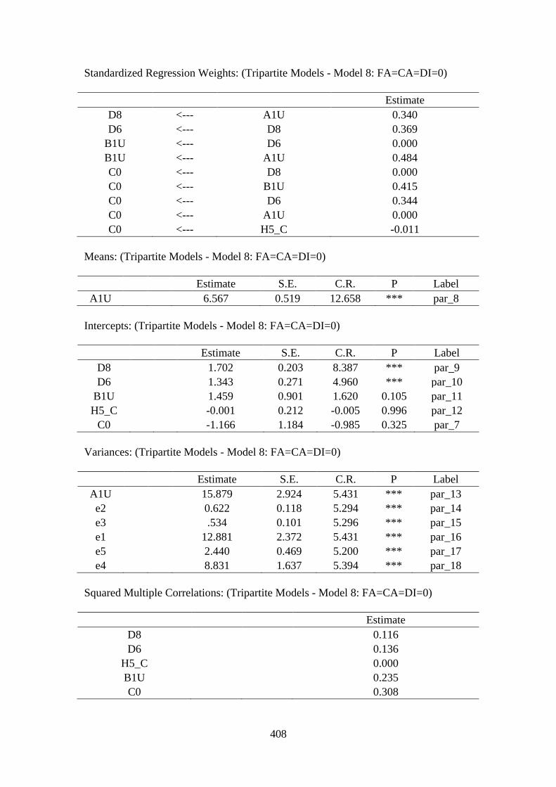
408
Standardized Regression Weights: (Tripartite Models - Model 8: FA=CA=DI=0)
Estimate
D8 <--- A1U 0.340
D6 <--- D8 0.369
B1U <--- D6 0.000
B1U <--- A1U 0.484
C0 <--- D8 0.000
C0 <--- B1U 0.415
C0 <--- D6 0.344
C0 <--- A1U 0.000
C0 <--- H5_C -0.011
Means: (Tripartite Models - Model 8: FA=CA=DI=0)
Estimate S.E. C.R. P Label
A1U
6.567 0.519 12.658 *** par_8
Intercepts: (Tripartite Models - Model 8: FA=CA=DI=0)
Estimate S.E. C.R. P Label
D8
1.702 0.203 8.387 *** par_9
D6
1.343 0.271 4.960 *** par_10
B1U
1.459 0.901 1.620 0.105 par_11
H5_C
-0.001 0.212 -0.005 0.996 par_12
C0
-1.166 1.184 -0.985 0.325 par_7
Variances: (Tripartite Models - Model 8: FA=CA=DI=0)
Estimate S.E. C.R. P Label
A1U
15.879 2.924 5.431 *** par_13
e2
0.622 0.118 5.294 *** par_14
e3
.534 0.101 5.296 *** par_15
e1
12.881 2.372 5.431 *** par_16
e5
2.440 0.469 5.200 *** par_17
e4
8.831 1.637 5.394 *** par_18
Squared Multiple Correlations: (Tripartite Models - Model 8: FA=CA=DI=0)
Estimate
D8
0.116
D6
0.136
H5_C
0.000
B1U
0.235
C0
0.308

409
Matrices (Tripartite Models - Model 8: FA=CA=DI=0)
Total Effects (Tripartite Models - Model 8: FA=CA=DI=0)
A1U D8 D6 H5_C B1U
D8 0.072 0.000 0.000 0.000 0.000
D6 0.025 0.346 0.000 0.000 0.000
B1U 0.499 0.000 0.000 0.000 0.000
C0 0.219 0.540 1.562 -0.024 0.361
Standardized Total Effects (Tripartite Models - Model 8: FA=CA=DI=0)
A1U D8 D6 H5_C B1U
D8 0.340 0.000 0.000 0.000 0.000
D6 0.126 0.369 0.000 0.000 0.000
B1U 0.484 0.000 0.000 0.000 0.000
C0 0.244 0.127 0.344 -0.011 0.415
Direct Effects (Tripartite Models - Model 8: FA=CA=DI=0)
A1U D8 D6 H5_C B1U
D8 0.072 0.000 0.000 0.000 0.000
D6 0.000 0.346 0.000 0.000 0.000
B1U 0.499 0.000 0.000 0.000 0.000
C0 0.000 0.000 1.562 -0.024 0.361
Standardized Direct Effects (Tripartite Models - Model 8: FA=CA=DI=0)
A1U D8 D6 H5_C B1U
D8 0.340 0.000 0.000 0.000 0.000
D6 0.000 0.369 0.000 0.000 0.000
B1U 0.484 0.000 0.000 0.000 0.000
C0 0.000 0.000 0.344 -0.011 0.415
Indirect Effects (Tripartite Models - Model 8: FA=CA=DI=0)
A1U D8 D6 H5_C B1U
D8 0.000 0.000 0.000 0.000 0.000
D6 0.025 0.000 0.000 0.000 0.000
B1U 0.000 0.000 0.000 0.000 0.000
C0 0.219 0.540 0.000 0.000 0.000

410
Standardized Indirect Effects (Tripartite Models - Model 8: FA=CA=DI=0)
A1U D8 D6 H5_C B1U
D8 0.000 0.000 0.000 0.000 0.000
D6 0.126 0.000 0.000 0.000 0.000
B1U 0.000 0.000 0.000 0.000 0.000
C0 0.244 0.127 0.000 0.000 0.000
Minimization History (Model 8: FA=CA=DI=0)
Iteration
Negative
eigenvalues
Condition
# Diameter F NTries Ratio
0 e 0 370.752 9999.000 82.351 0 9999.000
1 e 0 105.794 1.513 41.481 3 0.000
2 e 0 92.990 0.993 13.034 1 0.973
3 e 0 91.609 0.198 8.813 1 1.166
4 e 0 91.874 00.073 8.360 1 1.099
5 e 0 93.467 00.013 8.347 1 1.025
6 e 0 92.283 .001 8.347 1 1.001

411
Pairwise Parameter Comparisons (Model 8: FA=CA=DI=0)
Variance-covariance Matrix of Estimates (Model 8: FA=CA=DI=0)
FC FI CD IA DA LA par_7 par_8 par_9 par_10 par_11 par_12 par_13 par_14 par_15 par_16 par_17 par_18
FC 0.001
FI 0.000 0.014
CD 0.000 0.000 0.014
IA 0.000 0.000 0.000 0.009
DA 0.000 0.000 0.000 -0.003 0.253
LA 0.000 0.000 0.000 0.000 0.000 0.067
par_7 0.000 0.000 0.000 -0.036 -0.515 0.000 1.402
par_8 0.000 0.000 0.000 0.000 0.000 0.000 0.000 0.269
par_9 -0.005 0.000 0.000 0.000 0.000 0.000 -0.001 0.000 0.041
par_10 0.000 0.000 -0.029 0.000 0.000 0.000 -0.002 0.000 0.000 0.073
par_11 0.000 -0.090 0.000 0.000 0.000 0.000 0.000 0.000 0.000 0.000 0.811
par_12 0.000 0.000 0.000 0.000 0.000 0.000 0.000 0.000 0.000 0.000 0.000 0.045
par_13 0.000 0.000 0.000 0.000 0.000 0.000 0.000 0.000 0.000 0.000 0.000 0.000 8.547
par_14 0.000 0.000 0.000 0.000 0.000 0.000 0.000 0.000 0.000 0.000 0.000 0.000 0.000 0.014
par_15 0.000 0.000 0.000 0.000 0.000 0.000 0.000 0.000 0.000 0.000 0.000 0.000 0.000 0.000 0.010
par_16 0.000 0.000 0.000 0.000 0.000 0.000 0.000 0.000 0.000 0.000 0.000 0.000 0.000 0.000 0.000 5.624
par_17 0.000 0.000 0.000 0.000 0.000 0.000 0.000 0.000 0.000 0.000 0.000 0.000 0.000 0.000 0.000 0.000 0.220
par_18 0.000 0.000 -0.001 0.000 -0.018 0.001 0.036 0.000 0.000 0.001 0.000 0.000 0.000 0.000 -0.001 0.000 0.000 2.681
Correlations of Estimates (Model 8: FA=CA=DI=0)
FC FI CD IA DA LA par_7 par_8 par_9 par_10 par_11 par_12 par_13 par_14 par_15 par_16 par_17 par_18
FC 1.000
FI 0.000 1.000
CD -0.001 0.000 1.000
IA -0.003 0.000 -0.003 1.000
DA -0.001 0.000 -0.002 -0.062 1.000
LA 0.000 0.000 0.000 0.000 0.000 1.000
par_7 0.002 0.000 0.003 -0.324 -0.866 0.000 1.000
par_8 0.000 0.000 0.000 0.000 0.000 0.000 0.000 1.000
par_9 -0.855 0.000 0.001 0.003 0.001 0.000 -0.003 0.000 1.000
par_10 0.001 0.000 -0.933 0.002 0.002 0.000 -0.005 0.000 -0.001 1.000
par_11 0.000 -0.855 0.000 0.000 0.000 0.000 0.000 0.000 0.000 0.000 1.000
par_12 0.000 0.000 0.000 0.000 0.000 0.000 0.000 0.000 0.000 0.000 0.000 1.000
par_13 00.000 0.000 0.000 0.000 0.000 0.000 0.000 0.000 0.000 0.000 0.000 0.000 1.000
par_14 0.000 0.000 0.000 0.000 0.000 0.000 0.000 0.000 0.000 0.000 0.000 0.000 0.000 1.000
par_15 0.000 0.000 0.000 0.000 -0.003 0.000 0.003 0.000 0.000 0.000 0.000 0.000 0.000 0.000 1.000
par_16 0.000 0.000 0.000 0.000 0.000 0.000 0.000 0.000 0.000 0.000 0.000 0.000 0.000 0.000 0.000 1.000
par_17 0.000 0.000 0.000 0.000 0.000 0.000 0.000 0.000 0.000 0.000 0.000 0.000 0.000 0.000 0.000 0.000 1.000
par_18 0.000 0.000 -0.003 0.001 -0.022 0.001 0.019 0.000 0.000 .003 0.000 0.000 0.000 -0.001 -0.006 0.000 0.000 1.000

412
Model 9: FA=CA=DA=0 (Model 9: FA=CA=DA=0)
Notes for Model (Model 9: FA=CA=DA=0)
Computation of degrees of freedom (Model 9: FA=CA=DA=0)
Number of distinct sample moments: 27
Number of distinct parameters to be estimated: 18
Degrees of freedom (27 - 18): 9
Result (Model 9: FA=CA=DA=0)
Minimum was achieved
Chi-square = 12.073
Degrees of freedom = 9
Probability level = .209
Tripartite Models (Tripartite Models - Model 9: FA=CA=DA=0)
Estimates (Tripartite Models - Model 9: FA=CA=DA=0)
Scalar Estimates (Tripartite Models - Model 9: FA=CA=DA=0)
Maximum Likelihood Estimates
Regression Weights: (Tripartite Models - Model 9: FA=CA=DA=0)
Estimate S.E. C.R. P Label
D8 <--- A1U 0.071 0.026 2.690 0.007 FC
D6 <--- D8 0.345 0.117 2.956 0.003 CD
B1U <--- D6 1.298 0.587 2.212 0.027 DI
B1U <--- A1U 0.435 0.114 3.820 *** FI
C0 <--- D8 0.000
C0 <--- B1U 0.467 0.102 4.553 *** IA
C0 <--- D6 0.000
C0 <--- A1U 0.000
C0 <--- H5_C 0.005 0.277 0.017 0.986 LA

413
Standardized Regression Weights: (Tripartite Models - Model 9: FA=CA=DA=0)
Estimate
D8 <--- A1U 0.338
D6 <--- D8 0.367
B1U <--- D6 0.253
B1U <--- A1U 0.428
C0 <--- D8 0.000
C0 <--- B1U 0.510
C0 <--- D6 0.000
C0 <--- A1U 0.000
C0 <--- H5_C 0.002
Means: (Tripartite Models - Model 9: FA=CA=DA=0)
Estimate S.E. C.R. P Label
A1U
6.567 0.519 12.658 *** par_8
Intercepts: (Tripartite Models - Model 9: FA=CA=DA=0)
Estimate S.E. C.R. P Label
D8
1.705 0.203 8.395 *** par_9
D6
1.342 0.272 40.938 *** par_10
B1U
-.838 1.427 -0.587 0.557 par_11
H5_C
0.000 0.212 0.001 0.999 par_12
C0
1.608 0.638 2.520 0.012 par_7
Variances: (Tripartite Models - Model 9: FA=CA=DA=0)
Estimate S.E. C.R. P Label
A1U
15.879 2.924 5.431 *** par_13
e2
0.623 0.118 5.294 *** par_14
e3
0.537 0.102 5.295 *** par_15
e1
11.898 2.199 5.410 *** par_16
e5
2.440 0.469 5.200 *** par_17
e4
10.154 1.869 5.431 *** par_18

414
Squared Multiple Correlations: (Tripartite Models - Model 9: FA=CA=DA=0)
Estimate
D8
0.114
D6
0.135
H5_C
0.000
B1U
0.274
C0
0.260
Matrices (Tripartite Models - Model 9: FA=CA=DA=0)
Total Effects (Tripartite Models - Model 9: FA=CA=DA=0)
A1U D8 D6 H5_C B1U
D8 0.071 0.000 0.000 0.000 0.000
D6 0.025 0.345 0.000 0.000 0.000
B1U 0.467 0.448 1.298 0.000 0.000
C0 0.218 0.209 0.606 0.005 0.467
Standardized Total Effects (Tripartite Models - Model 9: FA=CA=DA=0)
A1U D8 D6 H5_C B1U
D8 0.338 0.000 0.000 0.000 0.000
D6 0.124 0.367 0.000 0.000 0.000
B1U 0.459 0.093 0.253 0.000 0.000
C0 0.234 0.047 0.129 0.002 0.510
Direct Effects (Tripartite Models - Model 9: FA=CA=DA=0)
A1U D8 D6 H5_C B1U
D8 0.071 0.000 0.000 0.000 0.000
D6 0.000 0.345 0.000 0.000 0.000
B1U 0.435 0.000 1.298 0.000 0.000
C0 0.000 0.000 0.000 0.005 0.467
Standardized Direct Effects (Tripartite Models - Model 9: FA=CA=DA=0)
A1U D8 D6 H5_C B1U
D8 0.338 0.000 0.000 0.000 0.000
D6 0.000 0.367 0.000 0.000 0.000
B1U 0.428 0.000 0.253 0.000 0.000
C0 0.000 0.000 0.000 0.002 0.510

415
Indirect Effects (Tripartite Models - Model 9: FA=CA=DA=0)
A1U D8 D6 H5_C B1U
D8 0.000 0.000 0.000 0.000 0.000
D6 0.025 0.000 0.000 0.000 0.000
B1U 0.032 0.448 0.000 0.000 0.000
C0 0.218 0.209 0.606 0.000 0.000
Standardized Indirect Effects (Tripartite Models - Model 9: FA=CA=DA=0)
A1U D8 D6 H5_C B1U
D8 0.000 0.000 0.000 0.000 0.000
D6 0.124 0.000 0.000 0.000 0.000
B1U 0.031 0.093 0.000 0.000 0.000
C0 0.234 0.047 0.129 0.000 0.000
Minimization History (Model 9: FA=CA=DA=0)
Iteration
Negative
eigenvalues Condition # Diameter F NTries Ratio
0 e 0 246.371 9999.000 85.035 0 9999.000
1 e 0 107.280 2.079 64.614 2 0.000
2 e 0 96.446 0.414 28.956 1 1.241
3 e 0 96.553 0.185 16.694 1 1.253
4 e 0 98.071 0.124 12.844 1 1.218
5 e 0 97.877 0.078 12.116 1 1.139
6 e 0 97.756 0.025 12.074 1 1.045
7 e 0 98.620 0.002 12.073 1 1.004
8 e 0 98.624 0.000 12.073 1 1.000

416
Pairwise Parameter Comparisons (Model 9: FA=CA=DA=0)
Variance-covariance Matrix of Estimates (Model 9: FA=CA=DA=0)
DI FC FI CD IA LA par_7 par_8 par_9 par_10 par_11 par_12 par_13 par_14 par_15 par_16 par_17 par_18
DI 0.345
FC 0.000 0.001
FI -0.008 0.000 0.013
CD 0.000 0.000 0.000 0.014
IA 0.000 0.000 0.000 0.000 0.011
LA 0.000 0.000 0.000 0.000 0.000 0.077
par_7 0.000 0.000 0.000 0.000 -0.050 0.000 0.407
par_8 0.000 0.000 0.000 0.000 0.000 0.000 0.000 0.269
par_9 0.000 -0.005 0.000 0.000 0.000 0.000 0.000 0.000 0.041
par_10 0.000 0.000 0.000 -0.030 0.000 0.000 0.000 0.000 0.000 0.074
par_11 -0.665 0.000 -0.067 0.000 0.000 0.000 0.000 0.000 -0.001 -0.002 20.037
par_12 0.000 0.000 0.000 0.000 0.000 0.000 0.000 0.000 0.000 0.000 0.000 0.045
par_13 0.000 0.000 0.000 0.000 0.000 0.000 0.000 0.000 0.000 0.000 0.000 0.000 8.547
par_14 0.000 0.000 0.000 0.000 0.000 0.000 0.000 0.000 0.000 0.000 0.000 0.000 0.000 0.014
par_15 0.000 0.000 0.000 0.000 0.000 0.000 0.000 0.000 0.000 0.000 0.000 0.000 0.000 0.000 0.010
par_16 -0.023 0.000 0.001 0.000 0.000 0.000 0.000 0.000 0.000 0.001 0.045 0.000 0.000 0.000 -0.001 4.838
par_17 0.000 0.000 0.000 0.000 0.000 0.000 0.000 0.000 0.000 0.000 0.000 0.000 0.000 0.000 0.000 0.000 0.220
par_18 0.000 0.000 0.000 0.000 0.000 0.000 0.000 0.000 0.000 0.000 0.000 0.000 0.000 0.000 0.000 0.000 0.000 3.495
Correlations of Estimates (Model 9: FA=CA=DA=0)
DI FC FI CD IA LA par_7 par_8 par_9 par_10 par_11 par_12 par_13 par_14 par_15 par_16 par_17 par_18
DI 1.000
FC 0.000 1.000
FI -0.127 -0.005 1.000
CD -0.001 0.000 -0.004 1.000
IA 0.000 0.000 0.000 0.000 1.000
LA 0.000 0.000 0.000 0.000 0.000 1.000
par_7 0.000 0.000 0.000 0.000 -0.760 0.000 1.000
par_8 0.000 0.000 0.000 0.000 0.000 0.000 0.000 1.000
par_9 0.000 -0.855 0.004 0.000 0.000 0.000 0.000 0.000 1.000
par_10 0.001 0.000 0.004 -0.933 0.000 0.000 0.000 0.000 -0.001 1.000
par_11 -0.794 0.003 -0.415 0.003 0.000 0.000 0.000 0.000 -0.003 -0.004 1.000
par_12 0.000 0.000 0.000 0.000 0.000 0.000 0.000 0.000 0.000 0.000 0.000 1.000
par_13 0.000 0.000 0.000 0.000 0.000 0.000 0.000 0.000 0.000 0.000 0.000 0.000 1.000
par_14 0.000 0.000 0.000 0.000 0.000 0.000 0.000 0.000 0.000 0.000 0.000 0.000 0.000 1.000
par_15 -0.001 0.000 0.000 0.000 0.000 0.000 0.000 0.000 0.000 0.000 0.001 0.000 0.000 0.000 1.000
par_16 -0.018 0.000 0.002 -0.002 0.000 0.000 0.000 0.000 0.000 0.002 0.014 0.000 0.000 0.000 -0.003 1.000
par_17 0.000 0.000 0.000 0.000 0.000 0.000 0.000 0.000 0.000 0.000 0.000 0.000 0.000 0.000 0.000 0.000 1.000
par_18 0.000 0.000 0.000 0.000 0.000 0.000 0.000 0.000 0.000 0.000 0.000 0.000 0.000 0.000 0.000 0.000 0.000 1.000

417
Model 10: FA=CA=IA=0 (Model 10: FA=CA=IA=0)
Notes for Model (Model 10: FA=CA=IA=0)
Computation of degrees of freedom (Model 10: FA=CA=IA=0)
Number of distinct sample moments: 27
Number of distinct parameters to be estimated: 18
Degrees of freedom (27 - 18): 9
Result (Model 10: FA=CA=IA=0)
Minimum was achieved
Chi-square = 14.541
Degrees of freedom = 9
Probability level = .104
Tripartite Models (Tripartite Models - Model 10: FA=CA=IA=0)
Estimates (Tripartite Models - Model 10: FA=CA=IA=0)
Scalar Estimates (Tripartite Models - Model 10: FA=CA=IA=0)
Maximum Likelihood Estimates
Regression Weights: (Tripartite Models - Model 10: FA=CA=IA=0)
Estimate S.E. C.R. P Label
D8 <--- A1U 0.071 0.026 2.684 0.007 FC
D6 <--- D8 0.348 0.117 2.969 0.003 CD
B1U <--- D6 1.403 0.576 2.436 0.015 DI
B1U <--- A1U 0.430 0.113 3.810 *** FI
C0 <--- D8 0.000
C0 <--- B1U 0.000
C0 <--- D6 2.304 0.539 4.271 *** DA
C0 <--- A1U 0.000
C0 <--- H5_C -0.070 0.283 -0.247 0.805 LA

418
Standardized Regression Weights: (Tripartite Models - Model 10: FA=CA=IA=0)
Estimate
D8 <--- A1U 0.337
D6 <--- D8 0.368
B1U <--- D6 0.275
B1U <--- A1U 0.424
C0 <--- D8 0.000
C0 <--- B1U 0.000
C0 <--- D6 0.492
C0 <--- A1U 0.000
C0 <--- H5_C -0.029
Means: (Tripartite Models - Model 10: FA=CA=IA=0)
Estimate S.E. C.R. P Label
A1U
6.567 0.519 12.658 *** par_8
Intercepts: (Tripartite Models - Model 10: FA=CA=IA=0)
Estimate S.E. C.R. P Label
D8
1.700 0.203 8.368 *** par_9
D6
1.320 0.272 4.848 *** par_10
B1U
-1.003 1.398 -0.718 0.473 par_11
H5_C
-0.001 0.212 -0.006 0.996 par_12
C0
-0.963 1.197 -0.805 0.421 par_7
Variances: (Tripartite Models - Model 10: FA=CA=IA=0)
Estimate S.E. C.R. P Label
A1U
15.879 2.924 5.431 *** par_13
e2
0.624 0.118 5.294 *** par_14
e3
0.544 0.103 5.303 *** par_15
e1
11.716 2.165 5.411 *** par_16
e5
2.441 0.469 5.200 *** par_17
e4
10.470 1.948 5.376 *** par_18
Squared Multiple Correlations: (Tripartite Models - Model 10: FA=CA=IA=0)
Estimate
D8
0.114
D6
0.136
H5_C
0.000
B1U
0.284
C0
0.243

419
Matrices (Tripartite Models - Model 10: FA=CA=IA=0)
Total Effects (Tripartite Models - Model 10: FA=CA=IA=0)
A1U D8 D6 H5_C B1U
D8 0.071 0.000 0.000 0.000 0.000
D6 0.025 0.348 0.000 0.000 0.000
B1U 0.465 0.489 1.403 0.000 0.000
C0 0.057 0.803 2.304 -0.070 0.000
Standardized Total Effects (Tripartite Models - Model 10: FA=CA=IA=0)
A1U D8 D6 H5_C B1U
D8 0.337 0.000 0.000 0.000 0.000
D6 0.124 0.368 0.000 0.000 0.000
B1U 0.458 0.101 0.275 0.000 0.000
C0 0.061 0.181 0.492 -0.029 0.000
Direct Effects (Tripartite Models - Model 10: FA=CA=IA=0)
A1U D8 D6 H5_C B1U
D8 0.071 0.000 0.000 0.000 0.000
D6 0.000 0.348 0.000 0.000 0.000
B1U 0.430 0.000 1.403 0.000 0.000
C0 0.000 0.000 2.304 -0.070 0.000
Standardized Direct Effects (Tripartite Models - Model 10: FA=CA=IA=0)
A1U D8 D6 H5_C B1U
D8 0.337 0.000 0.000 0.000 0.000
D6 0.000 0.368 0.000 0.000 0.000
B1U 0.424 0.000 0.275 0.000 0.000
C0 0.000 0.000 0.492 -0.029 0.000
Indirect Effects (Tripartite Models - Model 10: FA=CA=IA=0)
A1U D8 D6 H5_C B1U
D8 0.000 0.000 0.000 0.000 0.000
D6 0.025 0.000 0.000 0.000 0.000
B1U 0.035 0.489 0.000 0.000 0.000
C0 0.057 0.803 0.000 0.000 0.000

420
Standardized Indirect Effects (Tripartite Models - Model 10: FA=CA=IA=0)
A1U D8 D6 H5_C B1U
D8 0.000 0.000 0.000 0.000 0.000
D6 0.124 0.000 0.000 0.000 0.000
B1U 0.034 0.101 0.000 0.000 0.000
C0 0.061 0.181 0.000 0.000 0.000
Minimization History (Model 10: FA=CA=IA=0)
Iteration
Negative
eigenvalues
Condition
# Diameter F NTries Ratio
0 e 0 285.157 9999.000 89.417 0 9999.000
1 e 0 154.163 1.280 40.428 3 0.000
2 e 0 111.376 1.138 16.262 1 0.931
3 e 0 112.408 0.172 14.612 1 1.112
4 e 0 113.235 0.045 14.542 1 1.046
5 e 0 112.967 0.004 14.541 1 1.005
6 e 0 112.967 0.000 14.541 1 1.000

421
Pairwise Parameter Comparisons (Model 10: FA=CA=IA=0)
Variance-covariance Matrix of Estimates (Model 10: FA=CA=IA=0)
DI FC FI CD DA LA par_7 par_8 par_9 par_10 par_11 par_12 par_13 par_14 par_15 par_16 par_17 par_18
DI 0.332
FC 0.000 0.001
FI -0.008 0.000 0.013
CD 0.000 0.000 0.000 0.014
DA -0.001 0.000 0.000 0.000 0.291
LA 0.000 0.000 0.000 0.000 0.000 0.080
par_7 0.002 0.000 0.000 0.001 -0.604 0.000 1.432
par_8 0.000 0.000 0.000 0.000 0.000 0.000 0.000 0.269
par_9 0.000 -0.005 0.000 0.000 0.000 0.000 0.000 0.000 0.041
par_10 0.000 0.000 0.000 -0.030 0.001 0.000 -0.002 0.000 0.000 0.074
par_11 -0.634 0.000 -0.067 0.001 0.001 0.000 -0.001 0.000 -0.001 -0.002 1.954
par_12 0.000 0.000 0.000 0.000 0.000 0.000 0.000 0.000 0.000 0.000 0.000 0.045
par_13 0.000 0.000 0.000 0.000 0.000 0.000 0.000 0.000 0.000 0.000 0.000 0.000 8.547
par_14 0.000 0.000 0.000 0.000 0.000 0.000 0.000 0.000 0.000 0.000 0.000 0.000 0.000 0.014
par_15 0.000 0.000 0.000 0.000 0.000 0.000 0.001 0.000 0.000 0.000 0.000 0.000 0.000 0.000 0.011
par_16 -0.019 0.000 0.000 0.000 0.003 0.000 -0.005 0.000 0.000 0.001 0.036 0.000 0.000 0.000 -0.001 4.687
par_17 0.000 0.000 0.000 0.000 0.000 0.000 0.000 0.000 0.000 0.000 0.000 0.000 0.000 0.000 0.000 0.000 0.220
par_18 0.004 0.000 0.000 -0.001 -0.023 0.002 0.048 0.000 0.000 0.002 -0.008 0.000 0.000 0.000 -0.001 -0.004 0.000 3.794
Correlations of Estimates (Model 10: FA=CA=IA=0)
DI FC FI CD DA LA par_7 par_8 par_9 par_10 par_11 par_12 par_13 par_14 par_15 par_16 par_17 par_18
DI 1.000
FC 0.000 1.000
FI -0.126 -0.004 1.000
CD -0.002 -0.002 -0.003 1.000
DA -0.003 -0.001 0.001 -0.004 1.000
LA 0.000 0.000 0.000 0.000 0.000 1.000
par_7 0.003 0.001 -0.001 0.004 -0.935 0.000 1.000
par_8 0.000 0.000 0.000 0.000 0.000 0.000 0.000 1.000
par_9 0.000 -0.855 0.003 0.001 0.001 0.000 -0.002 0.000 1.000
par_10 0.002 0.002 0.003 -0.933 0.004 0.000 -0.006 0.000 -0.002 1.000
par_11 -0.788 0.002 -0.423 0.004 0.002 0.000 -0.001 0.000 -0.003 -0.005 1.000
par_12 0.000 0.000 0.000 0.000 0.000 0.000 0.001 0.000 0.000 0.000 0.000 1.000
par_13 0.000 0.000 0.000 0.000 0.000 0.000 0.000 0.000 0.000 0.000 0.000 0.000 1.000
par_14 -0.001 0.000 0.000 0.000 -0.001 0.000 0.001 0.000 0.000 0.000 0.000 0.000 0.000 1.000
par_15 -0.004 0.000 0.001 -0.002 -0.007 0.000 0.007 0.000 0.000 0.002 0.003 0.000 0.000 0.000 1.000
par_16 -0.015 0.000 0.002 -0.001 0.002 0.000 -0.002 0.000 0.000 0.001 0.012 0.000 0.000 0.000 -0.002 1.000
par_17 0.000 0.000 0.000 0.000 0.000 0.000 0.000 0.000 0.000 0.000 0.000 0.000 0.000 0.000 0.000 0.000 1.000
par_18 0.004 0.000 0.000 -0.003 -0.022 0.004 0.021 0.000 0.000 0.003 -0.003 0.000 0.000 -0.001 -0.007 -0.001 0.000 1.000

422
Model Fit Summary
CMIN
Model NPAR CMIN DF P CMIN/DF
Model 3: Composite (FA=CA=0) 19 3.589 8 0.892 0.449
Model 5: FA=CA=FI=0 18 16.040 9 0.066 1.782
Model 6: FA=CA=FC=0 18 10.544 9 0.308 1.172
Model 7: FA=CA=CD=0 18 11.704 9 0.231 1.300
Model 8: FA=CA=DI=0 18 8.347 9 0.500 0.927
Model 9: FA=CA=DA=0 18 12.073 9 0.209 1.341
Model 10: FA=CA=IA=0 18 14.541 9 0.104 1.616
Saturated model 27 .000 0
Independence model 6 65.563 21 0.000 3.122
Baseline Comparisons
Model NFI
Delta1
RFI
rho1
IFI
Delta2
TLI
rho2 CFI
Model 3: Composite (FA=CA=0) 0.945 0.856 1.077 1.260 1.000
Model 5: FA=CA=FI=0 0.755 0.429 0.876 0.631 0.842
Model 6: FA=CA=FC=0 0.839 0.625 0.973 0.919 0.965
Model 7: FA=CA=CD=0 0.821 0.583 0.952 0.858 .939
Model 8: FA=CA=DI=0 0.873 0.703 1.012 1.034 1.000
Model 9: FA=CA=DA=0 0.816 0.570 0.946 0.839 0.931
Model 10: FA=CA=IA=0 0.778 0.482 0.902 0.710 0.876
Saturated model 1.000
1.000
1.000
Independence model 0.000 0.000 0.000 0.000 0.000
Parsimony-Adjusted Measures
Model PRATIO PNFI PCFI
Model 3: Composite (FA=CA=0) 0.381 0.360 0.381
Model 5: FA=CA=FI=0 0.429 0.324 0.361
Model 6: FA=CA=FC=0 0.429 0.360 0.414
Model 7: FA=CA=CD=0 0.429 0.352 0.403
Model 8: FA=CA=DI=0 0.429 0.374 0.429
Model 9: FA=CA=DA=0 0.429 0.350 0.399
Model 10: FA=CA=IA=0 0.429 0.334 0.375
Saturated model 0.000 0.000 0.000
Independence model 1.000 0.000 0.000

423
NCP
Model NCP LO 90 HI 90
Model 3: Composite (FA=CA=0) 0.000 0.000 2.276
Model 5: FA=CA=FI=0 7.040 0.000 22.310
Model 6: FA=CA=FC=0 1.544 0.000 13.919
Model 7: FA=CA=CD=0 2.704 0.000 15.761
Model 8: FA=CA=DI=0 0.000 0.000 10.266
Model 9: FA=CA=DA=0 3.073 0.000 16.339
Model 10: FA=CA=IA=0 5.541 0.000 20.096
Saturated model 0.000 0.000 0.000
Independence model 44.563 23.861 72.881
FMIN
Model FMIN F0 LO 90 HI 90
Model 3: Composite (FA=CA=0) 0.061 0.000 0.000 0.039
Model 5: FA=CA=FI=0 0.272 0.119 0.000 0.378
Model 6: FA=CA=FC=0 0.179 0.026 0.000 0.236
Model 7: FA=CA=CD=0 0.198 0.046 0.000 0.267
Model 8: FA=CA=DI=0 0.141 0.000 0.000 0.174
Model 9: FA=CA=DA=0 0.205 0.052 0.000 0.277
Model 10: FA=CA=IA=0 0.246 0.094 0.000 0.341
Saturated model 0.000 0.000 0.000 0.000
Independence model 1.111 0.755 0.404 1.235
RMSEA
Model RMSEA LO 90 HI 90 PCLOSE
Model 3: Composite (FA=CA=0) 0.000 0.000 0.069 0.927
Model 5: FA=CA=FI=0 0.115 0.000 0.205 0.122
Model 6: FA=CA=FC=0 0.054 0.000 0.162 0.421
Model 7: FA=CA=CD=0 0.071 0.000 0.172 0.335
Model 8: FA=CA=DI=0 0.000 0.000 0.139 0.611
Model 9: FA=CA=DA=0 0.076 0.000 0.175 0.310
Model 10: FA=CA=IA=0 0.102 0.000 0.195 0.177
Independence model 0.190 0.139 0.243 0.000

424
AIC
Model AIC BCC
Model 3: Composite (FA=CA=0) 41.589 46.704
Model 5: FA=CA=FI=0 52.040 56.886
Model 6: FA=CA=FC=0 46.544 51.390
Model 7: FA=CA=CD=0 47.704 52.550
Model 8: FA=CA=DI=0 44.347 49.193
Model 9: FA=CA=DA=0 48.073 52.920
Model 10: FA=CA=IA=0 50.541 55.387
Saturated model 54.000 61.269
Independence model 77.563 79.178
ECVI
Model ECVI LO 90 HI 90 MECVI
Model 3: Composite (FA=CA=0) 0.705 0.780 0.818 0.792
Model 5: FA=CA=FI=0 0.882 0.763 1.141 0.964
Model 6: FA=CA=FC=0 0.789 0.763 0.999 0.871
Model 7: FA=CA=CD=0 0.809 0.763 1.030 0.891
Model 8: FA=CA=DI=0 0.752 0.763 0.937 0.834
Model 9: FA=CA=DA=0 0.815 0.763 1.040 0.897
Model 10: FA=CA=IA=0 0.857 0.763 1.103 0.939
Saturated model 0.915 0.915 0.915 1.038
Independence model 1.315 .964 1.795 1.342
HOELTER
Model HOELTER
.05
HOELTER
.01
Model 3: Composite (FA=CA=0) 255 331
Model 5: FA=CA=FI=0 63 80
Model 6: FA=CA=FC=0 95 122
Model 7: FA=CA=CD=0 86 110
Model 8: FA=CA=DI=0 120 154
Model 9: FA=CA=DA=0 83 106
Model 10: FA=CA=IA=0 69 88
Independence model 30 36

425
Nested Model Comparisons
Assuming model Model 3: Composite (FA=CA=0) to be correct:
Model DF CMIN P NFI
Delta-1
IFI
Delta-2
RFI
rho-1
TLI
rho2
Model 5: FA=CA=FI=0 1 12.452 0.000 0.190 0.216 0.427 0.628
Model 6: FA=CA=FC=0 1 6.955 0.008 0.106 0.121 0.232 0.341
Model 7: FA=CA=CD=0 1 8.115 0.004 0.124 0.141 0.273 0.401
Model 8: FA=CA=DI=0 1 4.759 0.029 0.073 0.083 0.153 0.226
Model 9: FA=CA=DA=0 1 8.485 0.004 0.129 0.147 0.286 0.421
Model 10: FA=CA=IA=0 1 10.953 0.001 0.167 0.190 0.374 0.550
Execution time summary
Minimization: 0.000
Miscellaneous: 0.459
Bootstrap: 0.000
Total: 0.459

426
APPENDIX K
WATER-COHERENT URBANISM MEASURES AND INTERVIEW
QUESTIONS
Variable: openness toward storing runoffs
1. Flood-prone cities are considering the following ways to address flooding issues in the
public spaces. How likely would you support storing 90% of the stormwater from public
roads and properties during storms by…
a. converting auto lanes to 1m deep canals with bike paths
□ Very (3) □ Somewhat (2) □ Not (1)
b. deepening existing canals from 1m to 3m □ Very (3) □ Somewhat (2) □ Not (1)
c. lowering the grounds of plazas and playgrounds □ Very (3) □ Somewhat (2) □ Not (1)
d. retrofitting plazas to float on top of water □ Very (3) □ Somewhat (2) □ Not (1)
e. retrofitting underground parking for storage □ Very (3) □ Somewhat (2) □ Not (1)
f. building big underground pipes for storage □ Very (3) □ Somewhat (2) □ Not (1)
g. Please specify or explain why you did not support any of the above solutions________
Variable: openness toward infiltrating runoffs
2. How likely would you support returning 90% of the stormwater from public roads and
properties after storms by…
a. converting auto lanes to creeks with bike paths □ Very (3) □ Somewhat (2) □ Not (1)
b. converting parking lots into parks □ Very (3) □ Somewhat (2) □ Not (1)
c. converting plazas into parks □ Very (3) □ Somewhat (2) □ Not (1)
d. making roads porous □ Very (3) □ Somewhat (2) □ Not (1)
e. Please specify or explain why you did not support any of the above solutions________
Variable: openness toward water transportation
3. How likely would you travel by water more…
a. if you had an amphibious car? □ Very (3) □ Somewhat (2) □ Not (1)
b. if water were near your home? □ Very (3) □ Somewhat (2) □ Not (1)
c. if water were near where you typically go? □ Very (3) □ Somewhat (2) □ Not (1)
d. if you could take your bicycle along? □ Very (3) □ Somewhat (2) □ Not (1)
e. if the water network were expanded? □ Very (3) □ Somewhat (2) □ Not (1)

427
f. if water movement generated energy? □ Very (3) □ Somewhat (2) □ Not (1)
g. if it improved water quality? □ Very (3) □ Somewhat (2) □ Not (1)
h. if there were more security docking? □ Very (3) □ Somewhat (2) □ Not (1)
i. if it improved your wellbeing? □ Very (3) □ Somewhat (2) □ Not (1)
j. if flood evacuation were likely in your area? □ Very (3) □ Somewhat (2) □ Not (1)
k. if there were no fuel cost? □ Very (3) □ Somewhat (2) □ Not (1)
l. if it reduced climate change impacts? □ Very (3) □ Somewhat (2) □ Not (1)
m. if it decreased sea level rise? □ Very (3) □ Somewhat (2) □ Not (1)
n. if it reduced risks of flooding in your city? □ Very (3) □ Somewhat (2) □ Not (1)
o. if it reduced risks of flooding in other cities? □ Very (3) □ Somewhat (2) □ Not (1)
Variable: openness toward canals and creeks
4. Would you like to see more canals or creeks…
a. supported floating parks? □ Very (3) □ Somewhat (2) □ Not (1)
b. supported floating greenhouses? □ Very (3) □ Somewhat (2) □ Not (1)
c. generated renewable energy? □ Very (3) □ Somewhat (2) □ Not (1)
d. supplied clean water? □ Very (3) □ Somewhat (2) □ Not (1)
e. reduced floods? □ Very (3) □ Somewhat (2) □ Not (1)
f. supported water transportation? □ Very (3) □ Somewhat (2) □ Not (1)
g. improved water quality? □ Very (3) □ Somewhat (2) □ Not (1)
h. supported floating bicycle paths? □ Very (3) □ Somewhat (2) □ Not (1)
i. supported floating traffic lanes? □ Very (3) □ Somewhat (2) □ Not (1)
j. supported boathouses? □ Very (3) □ Somewhat (2) □ Not (1)
k. reduced heat in urban areas? □ Very (3) □ Somewhat (2) □ Not (1)
l. if it reduced climate change impacts? □ Very (3) □ Somewhat (2) □ Not (1)
m.if it decreased sea level rise? □ Very (3) □ Somewhat (2) □ Not (1)
n. provided water during droughts? □ Very (3) □ Somewhat (2) □ Not (1)
o. supported vegetation? □ Very (3) □ Somewhat (2) □ Not (1)
a. were necessary for distributing water? □ Very (3) □ Somewhat (2) □ Not (1)
b. were necessary for distributing energy? □ Very (3) □ Somewhat (2) □ Not (1)
c. were necessary for distributing food? □ Very (3) □ Somewhat (2) □ Not (1)
d. supported wildlife? □ Very (3) □ Somewhat (2) □ Not (1)

428
e. returned stormwater to the ground? □ Very (3) □ Somewhat (2) □ Not (1)
f. supported floating parks? □ Very (3) □ Somewhat (2) □ Not (1)
g. were more straight? □ Very (3) □ Somewhat (2) □ Not (1)
h. were more meandering? □ Very (3) □ Somewhat (2) □ Not (1)
i. needed energy to keep water in it? □ Very (3) □ Somewhat (2) □ Not (1)
c. Assume response categories as equally spaced points along a Likert scale to generate
scores as shown above in parentheses. Use the average score across all responses to
create variable measure.

429
APPENDIX L
SKETCH MAP EVALUATION RUBRIC AND CODING SCHEME
Type Score Description
Declarative
Component
1 Show an impressionist sketch of landmark/node
characteristics.
Declarative
Relations
2 Illustrate randomly distributed landmarks/nodes
unconnected by paths.
Procedural
Component
3 Display landmarks/nodes as destinations connected by paths
yet with little information about pure path intersections or
wayside landmarks.
Procedural
Relations
4 Exhibit path segments without wayside landmarks but with
some pure path intersections that seem to have been drawn
from turn-by-turn instructions.
Hierarchical
Component
5 Reveal landmarks/nodes in proximity to major paths,
landmark, or nodes without enough pure path intersections
to enable shortcut-taking.
Hierarchical
Relations
6 Reveal landmarks/nodes in proximity to major paths,
landmarks, nodes with enough pure path intersections to
enable shortcut-taking.
Topological
Component
7 Delineate districts by continuous edges or the clustering of
landmarks/nodes.
Topological
Relations
8 Show a nested hierarchy of multiple districts delineated
based on continuous edges or the clustering of
landmarks/nodes.
Configurational
Component
7 Indicate a distinct form that resembles only a small part of
the city center.

430
Configurational
Relations
8 Capture the entire city structure as one single configuration
or a collective pattern greater than the sum of multiple
distinct forms.
Projective
Component
7 Conjecture abstract components from known topological or
configurational components instead of district-defining
edges on the ground.
Projective
Relations
8 Infer abstract relationships from known topological or
configurational relationships instead of actual physical
relationships between districts.
c. Code 1 or 0 for indicating correct or incorrect city identification.
d. Assume response categories as equally spaced points along a Likert scale to generate
scores as shown above in parentheses.
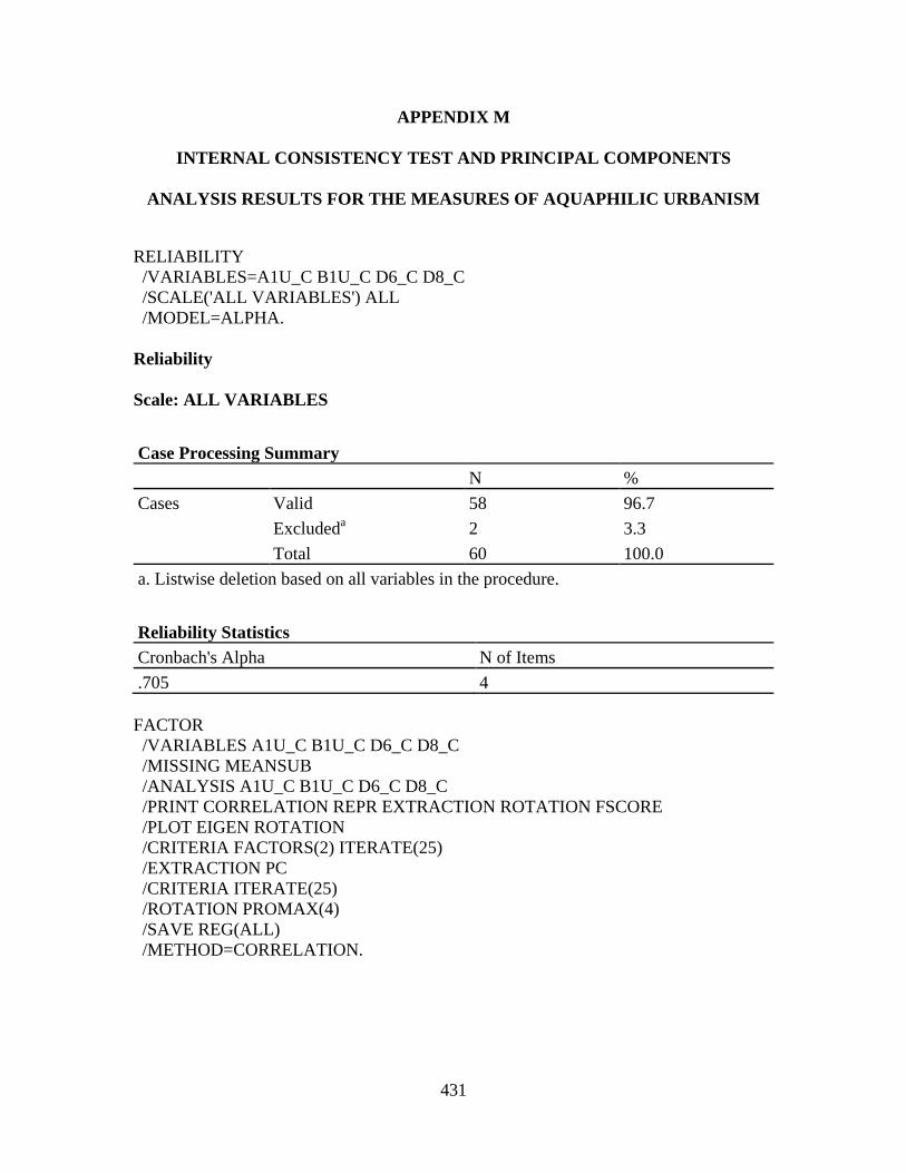
431
APPENDIX M
INTERNAL CONSISTENCY TEST AND PRINCIPAL COMPONENTS
ANALYSIS RESULTS FOR THE MEASURES OF AQUAPHILIC URBANISM
RELIABILITY
/VARIABLES=A1U_C B1U_C D6_C D8_C
/SCALE('ALL VARIABLES') ALL
/MODEL=ALPHA.
Reliability
Scale: ALL VARIABLES
Case Processing Summary
N %
Cases Valid 58 96.7
Excludeda 2 3.3
Total 60 100.0
a. Listwise deletion based on all variables in the procedure.
Reliability Statistics
Cronbach's Alpha N of Items
.705 4
FACTOR
/VARIABLES A1U_C B1U_C D6_C D8_C
/MISSING MEANSUB
/ANALYSIS A1U_C B1U_C D6_C D8_C
/PRINT CORRELATION REPR EXTRACTION ROTATION FSCORE
/PLOT EIGEN ROTATION
/CRITERIA FACTORS(2) ITERATE(25)
/EXTRACTION PC
/CRITERIA ITERATE(25)
/ROTATION PROMAX(4)
/SAVE REG(ALL)
/METHOD=CORRELATION.

432
Factor Analysis
Correlation Matrixa
Water-
Based
Familiarity
Water-
Based Place
Identity
Water-
Based Place
Dependence
Water-
Based
Comfort
Correlation Water-Based
Familiarity
1.000 .506 .264 .264
Water-Based Place
Identity
.506 1.000 .368 .368
Water-Based Place
Dependence
.264 .368 1.000 1.000
Water-Based
Comfort
.264 .368 1.000 1.000
a. This matrix is not positive definite.

433
Component Matrixa
Component
1 2
Water-Based Familiarity .571 .680
Water-Based Place Identity .669 .534
Water-Based Place Dependence .912 -.408
Water-Based Comfort .912 -.408
Extraction Method: Principal Component Analysis.
a. 2 components extracted.
Communalities
Extraction
Water-Based Familiarity .787
Water-Based Place Identity .732
Water-Based Place Dependence .998
Water-Based Comfort .998
Extraction Method: Principal Component Analysis.
Total Variance Explained
Component
Extraction Sums of Squared Loadings
Rotation Sums
of Squared
Loadingsa
Total % of Variance Cumulative % Total
1 2.435 60.880 60.880 2.209
2 1.080 27.008 87.888 1.759
Extraction Method: Principal Component Analysis.
a. When components are correlated, sums of squared loadings cannot be added to obtain
a total variance.

434
Reproduced Correlations
Water-
Based
Familiarity
Water-
Based
Place
Identity
Water-
Based Place
Dependence
Water-
Based
Comfort
Reproduced
Correlation
Water-Based
Familiarity
.787a .744 .243 .243
Water-Based
Place Identity
.744 .732a .392 .392
Water-Based
Place Dependence
.243 .392 .998a .998
Water-Based
Comfort
.243 .392 .998 .998a
Residualb Water-Based
Familiarity
-.239 .021 .021
Water-Based
Place Identity
-.239
-.024 -.024
Water-Based
Place Dependence
.021 -.024
.002
Water-Based
Comfort
.021 -.024 .002
Extraction Method: Principal Component Analysis.
a. Reproduced communalities
b. Residuals are computed between observed and reproduced correlations. There are 1
(16.0%) nonredundant residuals with absolute values greater than 0.05.
Pattern Matrixa
Component
1 2
Water-Based Familiarity -.084 .914
Water-Based Place Identity .102 .814
Water-Based Place Dependence .999 -.001
Water-Based Comfort .999 -.001
Extraction Method: Principal Component Analysis.
Rotation Method: Promax with Kaiser Normalization.a
a. Rotation converged in 3 iterations.

435
Structure Matrix
Component
1 2
Water-Based Familiarity .243 .884
Water-Based Place Identity .393 .850
Water-Based Place Dependence .999 .357
Water-Based Comfort .999 .357
Extraction Method: Principal Component Analysis.
Rotation Method: Promax with Kaiser Normalization.
Component Correlation Matrix
Component 1 2
1 1.000 .358
2 .358 1.000
Extraction Method: Principal Component Analysis.
Rotation Method: Promax with Kaiser Normalization.

436
Component Score Coefficient Matrix
Component
1 2
Water-Based Familiarity -.043 .610
Water-Based Place Identity .049 .543
Water-Based Place Dependence .496 -.002
Water-Based Comfort .496 -.002
Extraction Method: Principal Component Analysis.
Rotation Method: Promax with Kaiser Normalization.
Component Scores.
Component Score Covariance Matrix
Component 1 2
1 1.128 .715
2 .715 1.128
Extraction Method: Principal Component Analysis.
Rotation Method: Promax with Kaiser Normalization.
Component Scores.

437
APPENDIX N
INTERNAL CONSISTENCY TEST AND PRINCIPAL COMPONENTS
ANALYSIS RESULTS FOR THE MEASURES OF THE OPENNESS TOWARD
WATER-COHERENT URBANISM
RELIABILITY
/VARIABLES=F3_R_C F4_R_C G1_R_C G2_R_C
/SCALE('ALL VARIABLES') ALL
/MODEL=ALPHA.
Reliability
Scale: ALL VARIABLES
Case Processing Summary
N %
Cases Valid 42 70.0
Excludeda 18 30.0
Total 60 100.0
a. Listwise deletion based on all variables in the procedure.
Reliability Statistics
Cronbach's Alpha N of Items
.859 4
FACTOR
/VARIABLES F3_R_C F4_R_C G1_R_C G2_R_C
/MISSING MEANSUB
/ANALYSIS F3_R_C F4_R_C G1_R_C G2_R_C
/PRINT UNIVARIATE INITIAL CORRELATION REPR EXTRACTION
ROTATION FSCORE
/PLOT EIGEN ROTATION
/CRITERIA FACTORS(1) ITERATE(25)
/EXTRACTION PC
/CRITERIA ITERATE(25)
/ROTATION PROMAX(4)
/SAVE REG(ALL)
/METHOD=CORRELATION.

438
Factor Analysis
Descriptive Statistics
Mean Std. Deviationa Analysis N
a Missing N
Openness to Storing Public
Runoffs
.0000 .27989 50 2
Openness to Infiltrating
Public Runoffs
.0000 .30735 50 1
Openness to Water
Transportation
.0000 .24915 50 2
Openness to Canals and
Creeks
.0000 .18379 50 5
a. For each variable, missing values are replaced with the variable mean.
Correlation Matrix
Openness
to Storing
Public
Runoffs
Openness
to
Infiltrating
Public
Runoffs
Openness to
Water
Transportation
Openness
to Canals
and Creeks
Correlation Openness to Storing
Public Runoffs
1.000 .710 .540 .493
Openness to
Infiltrating Public
Runoffs
.710 1.000 .542 .487
Openness to Water
Transportation
.540 .542 1.000 .857
Openness to Canals
and Creeks
.493 .487 .857 1.000
Communalities
Initial Extraction
Openness to Storing Public Runoffs 1.000 .656
Openness to Infiltrating Public Runoffs 1.000 .653
Openness to Water Transportation 1.000 .781
Openness to Canals and Creeks 1.000 .728
Extraction Method: Principal Component Analysis.

439
Total Variance Explained
Component
Initial Eigenvalues Extraction Sums of Squared Loadings
Total
% of
Variance
Cumulative
% Total
% of
Variance
Cumulative
%
1 2.818 70.440 70.440 2.818 70.440 70.440
2 .752 18.810 89.250
3 .290 7.252 96.502
4 .140 3.498 100.000
Extraction Method: Principal Component Analysis.
Component Matrixa
Component
1
Openness to Storing Public Runoffs .810
Openness to Infiltrating Public Runoffs .808
Openness to Water Transportation .884
Openness to Canals and Creeks .853
Extraction Method: Principal Component Analysis.
a. 1 components extracted.

440
Reproduced Correlations
Openness
to Storing
Public
Runoffs
Openness
to
Infiltrating
Public
Runoffs
Openness to
Water
Transportation
Openness
to Canals
and
Creeks
Reproduced
Correlation
Openness to
Storing Public
Runoffs
.656a .654 .716 .691
Openness to
Infiltrating Public
Runoffs
.654 .653a .714 .689
Openness to
Water
Transportation
.716 .714 .781a .754
Openness to
Canals and
Creeks
.691 .689 .754 .728a
Residualb Openness to
Storing Public
Runoffs
.056 -.176 -.197
Openness to
Infiltrating Public
Runoffs
.056
-.172 -.203
Openness to
Water
Transportation
-.176 -.172
.103
Openness to
Canals and
Creeks
-.197 -.203 .103
Extraction Method: Principal Component Analysis.
a. Reproduced communalities
b. Residuals are computed between observed and reproduced correlations. There are 6
(100.0%) nonredundant residuals with absolute values greater than 0.05.

441
Component Score Coefficient Matrix
Component
1
Openness to Storing Public Runoffs .287
Openness to Infiltrating Public Runoffs .287
Openness to Water Transportation .314
Openness to Canals and Creeks .303
Extraction Method: Principal Component Analysis.
Rotation Method: Promax with Kaiser Normalization.
Component Scores.
Component Score Covariance Matrix
Component 1
1 1.000
Extraction Method: Principal Component Analysis.
Rotation Method: Promax with Kaiser Normalization.
Component Scores.

442
APPENDIX O
RESULTS OF MACRO-LEVEL MEDIATION ANALYSES
Run MATRIX procedure:
*****************************************************************
Preacher and Hayes (2008) SPSS Macro for Multiple Mediation
Written by Andrew F. Hayes, The Ohio State University
http://www.comm.ohio-state.edu/ahayes/
For details, see Preacher, K. J., & Hayes, A. F. (2008). Asymptotic
and resampling strategies for assessing and comparing indirect effects
in multiple mediator models. Behavior Research Methods, 40, 879-891.
*****************************************************************
------ END MATRIX -----
Model A
Dependent, Independent, and Proposed Mediator Variables:
DV = C0_C (allocentric aquaphilia)
IV = WQ (high or low water city)
MEDS = PCS_AU (aquaphilic urbanism)
Sample size
60
IV to Mediators (a paths)
Coeff se t p
PCS_AU 1.4604 .3512 4.1586 .0001
Direct Effects of Mediators on DV (b paths)
Coeff se t p
PCS_AU .3384 .0759 4.4568 .0000
Total Effect of IV on DV (c path)
Coeff se t p
WQ .6441 .2338 2.7553 .0078

443
Direct Effect of IV on DV (c' path)
Coeff se t p
WQ .1499 .2314 .6479 .5196
Model Summary for DV Model
R-sq Adj R-sq F df1 df2 p
.3443 .3212 14.9621 2.0000 57.0000 .0000
*****************************************************************
BOOTSTRAP RESULTS FOR INDIRECT EFFECTS
Indirect Effects of IV on DV through Proposed Mediators (ab paths)
Data Boot Bias SE
TOTAL .4942 .4979 .0037 .1791
PCS_AU .4942 .4979 .0037 .1791
Bias Corrected Confidence Intervals
Lower Upper
TOTAL .1913 .8970
PCS_AU .1913 .8970
*****************************************************************
Level of Confidence for Confidence Intervals:
95
Number of Bootstrap Resamples:
1000
********************************* NOTES********************************
------ END MATRIX -----
Model B
Dependent, Independent, and Proposed Mediator Variables:
DV = FAC1_2 (openness toward water-coherent urbanism)
IV = WQ (high or low water city)
MEDS = PCS_AU (aquaphilic urbanism)
Sample size
60
IV to Mediators (a paths)
Coeff se t p
PCS_AU 1.4604 .3512 4.1586 .0001

444
Direct Effects of Mediators on DV (b paths)
Coeff se t p
PCS_AU .1788 .0849 2.1057 .0396
Total Effect of IV on DV (c path)
Coeff se t p
WQ .3127 .2337 1.3378 .1862
Direct Effect of IV on DV (c' path)
Coeff se t p
WQ .0516 .2588 .1992 .8428
Model Summary for DV Model
R-sq Adj R-sq F df1 df2 p
.0999 .0684 3.1648 2.0000 57.0000 .0497
*****************************************************************
BOOTSTRAP RESULTS FOR INDIRECT EFFECTS
Indirect Effects of IV on DV through Proposed Mediators (ab paths)
Data Boot Bias SE
TOTAL .2611 .2717 .0106 .1487
PCS_AU .2611 .2717 .0106 .1487
Bias Corrected Confidence Intervals
Lower Upper
TOTAL .0314 .6102
PCS_AU .0314 .6102
*****************************************************************
Level of Confidence for Confidence Intervals:
95
Number of Bootstrap Resamples:
1000
********************************* NOTES********************************
------ END MATRIX -----
Model C
Dependent, Independent, and Proposed Mediator Variables:
DV = FAC1_2 (openness toward water-coherent urbanism)
IV = PCS_AU (aquaphilic urbanism)
MEDS = C0_C (allocentric aquaphilia)

445
Sample size
60
IV to Mediators (a paths)
Coeff se t p
C0_C .3620 .0663 5.4592 .0000
Direct Effects of Mediators on DV (b paths)
Coeff se t p
C0_C .3083 .1419 2.1730 .0339
Total Effect of IV on DV (c path)
Coeff se t p
PCS_AU .1869 .0739 2.5290 .0142
Direct Effect of IV on DV (c' path)
Coeff se t p
PCS_AU .0753 .0882 .8544 .3965
Model Summary for DV Model
R-sq Adj R-sq F df1 df2 p
.1682 .1390 5.7641 2.0000 57.0000 .0052
*****************************************************************
BOOTSTRAP RESULTS FOR INDIRECT EFFECTS
Indirect Effects of IV on DV through Proposed Mediators (ab paths)
Data Boot Bias SE
TOTAL .1116 .1070 -.0046 .0438
C0_C .1116 .1070 -.0046 .0438
Bias Corrected Confidence Intervals
Lower Upper
TOTAL .0413 .2225
C0_C .0413 .2225
*****************************************************************
Level of Confidence for Confidence Intervals:
95
Number of Bootstrap Resamples:
1000

446
********************************* NOTES********************************
------ END MATRIX -----
Model C1
Dependent, Independent, and Proposed Mediator Variables:
DV = FAC1_2 (openness toward water-coherent urbanism)
IV = FAC1_1 (water-based goal affordance)
MEDS = C0_C (allocentric aquaphilia)
Sample size
60
IV to Mediators (a paths)
Coeff se t p
C0_C .4716 .1090 4.3271 .0001
Direct Effects of Mediators on DV (b paths)
Coeff se t p
C0_C .3766 .1335 2.8215 .0066
Total Effect of IV on DV (c path)
Coeff se t p
FAC1_1 .1821 .1172 1.5534 .1258
Direct Effect of IV on DV (c' path)
Coeff se t p
FAC1_1 .0045 .1274 .0355 .9718
Model Summary for DV Model
R-sq Adj R-sq F df1 df2 p
.1576 .1280 5.3316 2.0000 57.0000 .0075
*****************************************************************
BOOTSTRAP RESULTS FOR INDIRECT EFFECTS
Indirect Effects of IV on DV through Proposed Mediators (ab paths)
Data Boot Bias SE
TOTAL .1776 .1746 -.0030 .0593
C0_C .1776 .1746 -.0030 .0593
Bias Corrected Confidence Intervals
Lower Upper
TOTAL .0878 .3381
C0_C .0878 .3381

447
*****************************************************************
Level of Confidence for Confidence Intervals:
95
Number of Bootstrap Resamples:
1000
********************************* NOTES********************************
------ END MATRIX -----
Model C2
Dependent, Independent, and Proposed Mediator Variables:
DV = FAC1_2 (openness toward water-coherent urbanism)
IV = FAC2_1 (water-based imageability)
MEDS = C0_C (allocentric aquaphilia)
Sample size
60
IV to Mediators (a paths)
Coeff se t p
C0_C .4511 .1105 4.0839 .0001
Direct Effects of Mediators on DV (b paths)
Coeff se t p
C0_C .2777 .1286 2.1594 .0350
Total Effect of IV on DV (c path)
Coeff se t p
FAC2_1 .3298 .1116 2.9568 .0045
Direct Effect of IV on DV (c' path)
Coeff se t p
FAC2_1 .2046 .1228 1.6663 .1011
Model Summary for DV Model
R-sq Adj R-sq F df1 df2 p
.1967 .1685 6.9788 2.0000 57.0000 .0019
*****************************************************************
BOOTSTRAP RESULTS FOR INDIRECT EFFECTS
Indirect Effects of IV on DV through Proposed Mediators (ab paths)
Data Boot Bias SE

448
TOTAL .1253 .1194 -.0059 .0541
C0_C .1253 .1194 -.0059 .0541
Bias Corrected Confidence Intervals
Lower Upper
TOTAL .0417 .2859
C0_C .0417 .2859
*****************************************************************
Level of Confidence for Confidence Intervals:
95
Number of Bootstrap Resamples:
1000
********************************* NOTES********************************

449
APPENDIX P
RESULTS OF MICRO-LEVEL MEDIATION ANALYSES
Run MATRIX procedure:
*****************************************************************
Preacher and Hayes (2008) SPSS Macro for Multiple Mediation
Written by Andrew F. Hayes, The Ohio State University
http://www.comm.ohio-state.edu/ahayes/
For details, see Preacher, K. J., & Hayes, A. F. (2008). Asymptotic
and resampling strategies for assessing and comparing indirect effects
in multiple mediator models. Behavior Research Methods, 40, 879-891.
*****************************************************************
------ END MATRIX -----
Model D
Dependent, Independent, and Proposed Mediator Variables:
DV = Co_2B (dua-perspective coherence)
IV = H2 (gender)
MEDS = A1_C (canal mappability)
B1_C (canal identifiability)
Statistical Controls:
CONTROL= D1_R (aquaphilia sensitivity baseline)
Sample size
51
IV to Mediators (a paths)
Coeff se t p
A1_C -1.5726 .8602 -1.8281 .0738
B1_C -1.3638 .6357 -2.1454 .0370
Direct Effects of Mediators on DV (b paths)
Coeff se t p
A1_C .3480 .1188 2.9305 .0053
B1_C -.2557 .1607 -1.5913 .1184

450
Total Effect of IV on DV (c path)
Coeff se t p
H2 -.4240 .6383 -.6643 .5097
Direct Effect of IV on DV (c' path)
Coeff se t p
H2 -.2255 .6305 -.3576 .7223
Partial Effect of Control Variables on DV
Coeff se t p
D1_R -.9604 .3800 -2.5275 .0150
Model Summary for DV Model
R-sq Adj R-sq F df1 df2 p
.2634 .1994 4.1128 4.0000 46.0000 .0062
*****************************************************************
BOOTSTRAP RESULTS FOR INDIRECT EFFECTS
Indirect Effects of IV on DV through Proposed Mediators (ab paths)
Data Boot Bias SE
TOTAL -.1985 -.2036 -.0051 .3236
A1_C -.5473 -.5619 -.0145 .3527
B1_C .3488 .3583 .0095 .2673
Bias Corrected Confidence Intervals
Lower Upper
TOTAL -.9262 .3735
A1_C -1.4828 -.0305
B1_C -.0106 1.0886
*****************************************************************
Level of Confidence for Confidence Intervals:
95
Number of Bootstrap Resamples:
1000
********************************* NOTES********************************
------ END MATRIX -----
Model E
Dependent, Independent, and Proposed Mediator Variables:
DV = Co_Ca (dual-perspective coherence)

451
IV = H2 (gender)
MEDS = A1_C (canal mappability)
Statistical Controls:
CONTROL= D1_R (aquaphilia sensitivity baseline)
Sample size
56
IV to Mediators (a paths)
Coeff se t p
A1_C -1.7472 .7955 -2.1965 .0325
Direct Effects of Mediators on DV (b paths)
Coeff se t p
A1_C .2114 .0406 5.2110 .0000
Total Effect of IV on DV (c path)
Coeff se t p
H2 -.6202 .2871 -2.1599 .0353
Direct Effect of IV on DV (c' path)
Coeff se t p
H2 -.2508 .2454 -1.0218 .3116
Partial Effect of Control Variables on DV
Coeff se t p
D1_R -.5530 .1469 -3.7649 .0004
Model Summary for DV Model
R-sq Adj R-sq F df1 df2 p
.4948 .4656 16.9757 3.0000 52.0000 .0000
*****************************************************************
BOOTSTRAP RESULTS FOR INDIRECT EFFECTS
Indirect Effects of IV on DV through Proposed Mediators (ab paths)
Data Boot Bias SE
TOTAL -.3694 -.3751 -.0056 .1752
A1_C -.3694 -.3751 -.0056 .1752
Bias Corrected Confidence Intervals
Lower Upper
TOTAL -.7524 -.0652
A1_C -.7524 -.0652

452
*****************************************************************
Level of Confidence for Confidence Intervals:
95
Number of Bootstrap Resamples:
1000
********************************* NOTES********************************
------ END MATRIX -----
Model F
Dependent, Independent, and Proposed Mediator Variables:
DV = Co_Ce (water-based egocentric coherence)
IV = H2 (gender)
MEDS = A1_C (canal mappability)
Statistical Controls:
CONTROL= D1_R (aquaphilia sensitivity baseline)
Sample size
51
IV to Mediators (a paths)
Coeff se t p
A1_C -1.5726 .8602 -1.8281 .0738
Direct Effects of Mediators on DV (b paths)
Coeff se t p
A1_C .1184 .0345 3.4325 .0013
Total Effect of IV on DV (c path)
Coeff se t p
H2 -.3644 .2274 -1.6025 .1156
Direct Effect of IV on DV (c' path)
Coeff se t p
H2 -.1783 .2125 -.8390 .4057
Partial Effect of Control Variables on DV
Coeff se t p
D1_R -.2867 .1301 -2.2036 .0325
Model Summary for DV Model
R-sq Adj R-sq F df1 df2 p

453
.3076 .2634 6.9596 3.0000 47.0000 .0006
*****************************************************************
BOOTSTRAP RESULTS FOR INDIRECT EFFECTS
Indirect Effects of IV on DV through Proposed Mediators (ab paths)
Data Boot Bias SE
TOTAL -.1861 -.1894 -.0033 .1055
A1_C -.1861 -.1894 -.0033 .1055
Bias Corrected Confidence Intervals
Lower Upper
TOTAL -.4428 -.0226
A1_C -.4428 -.0226
*****************************************************************
Level of Confidence for Confidence Intervals:
95
Number of Bootstrap Resamples:
1000
********************************* NOTES********************************
------ END MATRIX -----
Model G
Dependent, Independent, and Proposed Mediator Variables:
DV = Co_2B (dual-perspective coherence)
IV = TR (visitors or residents)
MEDS = A1_C (canal mappability)
B1_C (canal identifiability)
Statistical Controls:
CONTROL= D1_R (aquaphilia sensitivity baseline)
Sample size
51
IV to Mediators (a paths)
Coeff se t p
A1_C 1.3545 .7756 1.7464 .0871
B1_C -.3926 .5956 -.6591 .5130
Direct Effects of Mediators on DV (b paths)

454
Coeff se t p
A1_C .3016 .1252 2.4085 .0201
B1_C -.1913 .1631 -1.1730 .2468
Total Effect of IV on DV (c path)
Coeff se t p
TR 1.1271 .5531 2.0379 .0471
Direct Effect of IV on DV (c' path)
Coeff se t p
TR .6436 .5734 1.1224 .2675
Partial Effect of Control Variables on DV
Coeff se t p
D1_R -.9562 .3608 -2.6504 .0110
Model Summary for DV Model
R-sq Adj R-sq F df1 df2 p
.2811 .2185 4.4959 4.0000 46.0000 .0038
*****************************************************************
BOOTSTRAP RESULTS FOR INDIRECT EFFECTS
Indirect Effects of IV on DV through Proposed Mediators (ab paths)
Data Boot Bias SE
TOTAL .4835 .5202 .0366 .3182
A1_C .4085 .4366 .0281 .3135
B1_C .0751 .0836 .0085 .1562
Bias Corrected Confidence Intervals
Lower Upper
TOTAL -.0159 1.2576
A1_C -.0214 1.2210
B1_C -.1206 .5745
*****************************************************************
Level of Confidence for Confidence Intervals:
95
Number of Bootstrap Resamples:
1000
********************************* NOTES********************************
------ END MATRIX -----

455
Model H
Dependent, Independent, and Proposed Mediator Variables:
DV = Co_Ca (water-based allocentric coherence)
IV = TR (visitors or residents)
MEDS = A1_C (canal mappability)
Statistical Controls:
CONTROL= D1_R (aquaphilia sensitivity baseline)
Sample size
56
IV to Mediators (a paths)
Coeff se t p
A1_C 1.3247 .7272 1.8217 .0741
Direct Effects of Mediators on DV (b paths)
Coeff se t p
A1_C .2358 .0398 5.9235 .0000
Total Effect of IV on DV (c path)
Coeff se t p
TR .0329 .2702 .1219 .9035
Direct Effect of IV on DV (c' path)
Coeff se t p
TR -.2795 .2173 -1.2864 .2040
Partial Effect of Control Variables on DV
Coeff se t p
D1_R -.5998 .1404 -4.2708 .0001
Model Summary for DV Model
R-sq Adj R-sq F df1 df2 p
.5005 .4717 17.3707 3.0000 52.0000 .0000
*****************************************************************
BOOTSTRAP RESULTS FOR INDIRECT EFFECTS
Indirect Effects of IV on DV through Proposed Mediators (ab paths)
Data Boot Bias SE
TOTAL .3124 .3130 .0006 .1899
A1_C .3124 .3130 .0006 .1899
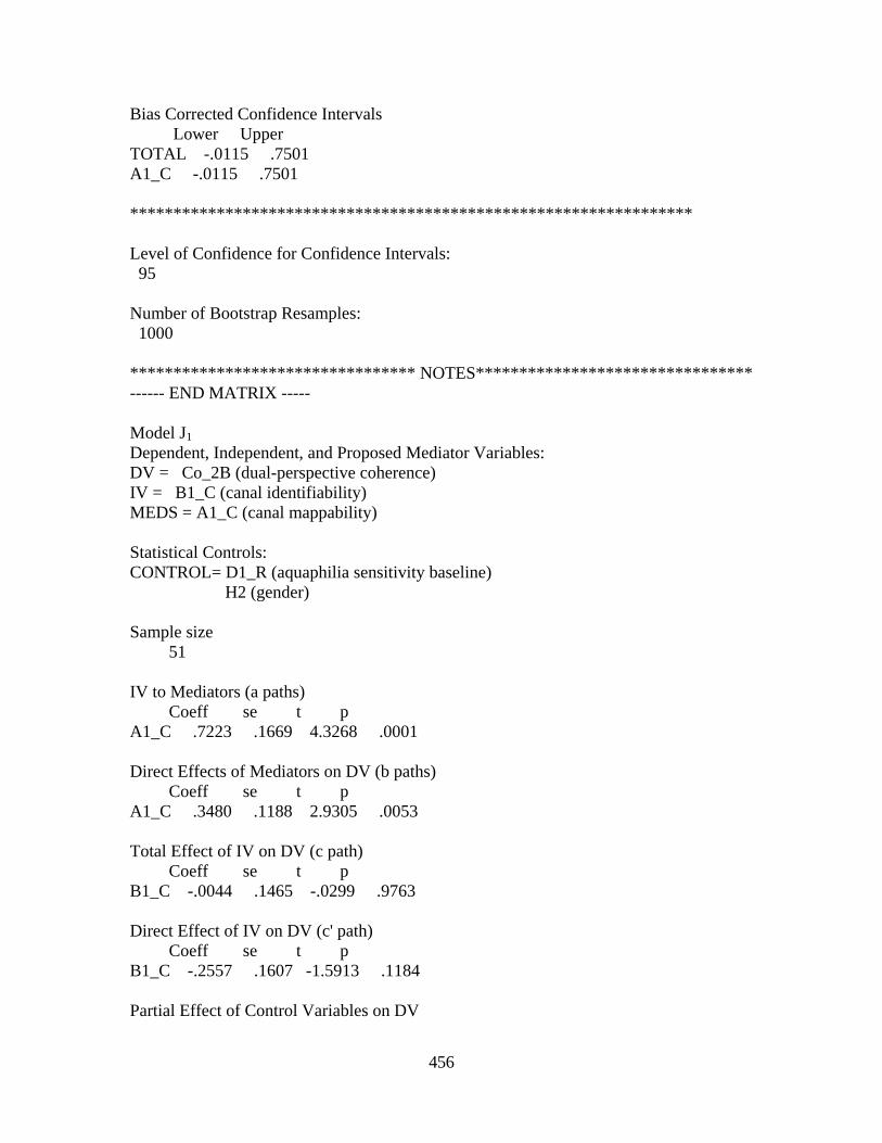
456
Bias Corrected Confidence Intervals
Lower Upper
TOTAL -.0115 .7501
A1_C -.0115 .7501
*****************************************************************
Level of Confidence for Confidence Intervals:
95
Number of Bootstrap Resamples:
1000
********************************* NOTES********************************
------ END MATRIX -----
Model J1
Dependent, Independent, and Proposed Mediator Variables:
DV = Co_2B (dual-perspective coherence)
IV = B1_C (canal identifiability)
MEDS = A1_C (canal mappability)
Statistical Controls:
CONTROL= D1_R (aquaphilia sensitivity baseline)
H2 (gender)
Sample size
51
IV to Mediators (a paths)
Coeff se t p
A1_C .7223 .1669 4.3268 .0001
Direct Effects of Mediators on DV (b paths)
Coeff se t p
A1_C .3480 .1188 2.9305 .0053
Total Effect of IV on DV (c path)
Coeff se t p
B1_C -.0044 .1465 -.0299 .9763
Direct Effect of IV on DV (c' path)
Coeff se t p
B1_C -.2557 .1607 -1.5913 .1184
Partial Effect of Control Variables on DV

457
Coeff se t p
D1_R -.9604 .3800 -2.5275 .0150
H2 -.2255 .6305 -.3576 .7223
Model Summary for DV Model
R-sq Adj R-sq F df1 df2 p
.2634 .1994 4.1128 4.0000 46.0000 .0062
*****************************************************************
BOOTSTRAP RESULTS FOR INDIRECT EFFECTS
Indirect Effects of IV on DV through Proposed Mediators (ab paths)
Data Boot Bias SE
TOTAL .2514 .2566 .0052 .1096
A1_C .2514 .2566 .0052 .1096
Bias Corrected Confidence Intervals
Lower Upper
TOTAL .0848 .5126
A1_C .0848 .5126
*****************************************************************
Level of Confidence for Confidence Intervals:
95
Number of Bootstrap Resamples:
1000
********************************* NOTES********************************
------ END MATRIX -----
Model J2
Dependent, Independent, and Proposed Mediator Variables:
DV = Co_2B (dual-perspective coherence)
IV = B1_C (canal identifiability)
MEDS = A1_C (canal mappability)
Statistical Controls:
CONTROL= D1_R (aquaphilia sensitivity baseline)
TR (visitors or residents)
Sample size
51

458
IV to Mediators (a paths)
Coeff se t p
A1_C .7981 .1501 5.3168 .0000
Direct Effects of Mediators on DV (b paths)
Coeff se t p
A1_C .3016 .1252 2.4085 .0201
Total Effect of IV on DV (c path)
Coeff se t p
B1_C .0494 .1353 .3653 .7165
Direct Effect of IV on DV (c' path)
Coeff se t p
B1_C -.1913 .1631 -1.1730 .2468
Partial Effect of Control Variables on DV
Coeff se t p
D1_R -.9562 .3608 -2.6504 .0110
TR .6436 .5734 1.1224 .2675
Model Summary for DV Model
R-sq Adj R-sq F df1 df2 p
.2811 .2185 4.4959 4.0000 46.0000 .0038
*****************************************************************
BOOTSTRAP RESULTS FOR INDIRECT EFFECTS
Indirect Effects of IV on DV through Proposed Mediators (ab paths)
Data Boot Bias SE
TOTAL .2407 .2551 .0145 .1243
A1_C .2407 .2551 .0145 .1243
Bias Corrected Confidence Intervals
Lower Upper
TOTAL .0634 .5555
A1_C .0634 .5555
*****************************************************************
Level of Confidence for Confidence Intervals:
95
Number of Bootstrap Resamples:
1000

459
********************************* NOTES********************************
------ END MATRIX -----
Model K1
Dependent, Independent, and Proposed Mediator Variables:
DV = Co_Ca (water-based allocentric coherence)
IV = B1_C (canal identifiability)
MEDS = A1_C (canal mappability)
Statistical Controls:
CONTROL= D1_R (aquaphilia sensitivity baseline)
H2 (gender)
Sample size
56
IV to Mediators (a paths)
Coeff se t p
A1_C .6605 .1618 4.0830 .0002
Direct Effects of Mediators on DV (b paths)
Coeff se t p
A1_C .1839 .0464 3.9607 .0002
Total Effect of IV on DV (c path)
Coeff se t p
B1_C .1964 .0613 3.2026 .0023
Direct Effect of IV on DV (c' path)
Coeff se t p
B1_C .0750 .0622 1.2045 .2340
Partial Effect of Control Variables on DV
Coeff se t p
D1_R -.5508 .1463 -3.7659 .0004
H2 -.2180 .2459 -.8864 .3796
Model Summary for DV Model
R-sq Adj R-sq F df1 df2 p
.5088 .4702 13.2048 4.0000 51.0000 .0000
*****************************************************************
BOOTSTRAP RESULTS FOR INDIRECT EFFECTS

460
Indirect Effects of IV on DV through Proposed Mediators (ab paths)
Data Boot Bias SE
TOTAL .1214 .1234 .0020 .0462
A1_C .1214 .1234 .0020 .0462
Bias Corrected Confidence Intervals
Lower Upper
TOTAL .0507 .2295
A1_C .0507 .2295
*****************************************************************
Level of Confidence for Confidence Intervals:
95
Number of Bootstrap Resamples:
1000
********************************* NOTES********************************
------ END MATRIX -----
Model K2
Dependent, Independent, and Proposed Mediator Variables:
DV = Co_Ca (water-based allocentric coherence)
IV = B1_C (canal identifiability)
MEDS = A1_C (canal mappability)
Statistical Controls:
CONTROL= D1_R (aquaphilia sensitivity baseline)
TR (visitors or residents)
Sample size
56
IV to Mediators (a paths)
Coeff se t p
A1_C .7850 .1494 5.2528 .0000
Direct Effects of Mediators on DV (b paths)
Coeff se t p
A1_C .2088 .0493 4.2342 .0001
Total Effect of IV on DV (c path)
Coeff se t p
B1_C .2251 .0612 3.6781 .0006

461
Direct Effect of IV on DV (c' path)
Coeff se t p
B1_C .0611 .0658 .9298 .3569
Partial Effect of Control Variables on DV
Coeff se t p
D1_R -.5922 .1409 -4.2041 .0001
TR -.2064 .2313 -.8924 .3764
Model Summary for DV Model
R-sq Adj R-sq F df1 df2 p
.5089 .4703 13.2102 4.0000 51.0000 .0000
*****************************************************************
BOOTSTRAP RESULTS FOR INDIRECT EFFECTS
Indirect Effects of IV on DV through Proposed Mediators (ab paths)
Data Boot Bias SE
TOTAL .1639 .1661 .0021 .0578
A1_C .1639 .1661 .0021 .0578
Bias Corrected Confidence Intervals
Lower Upper
TOTAL .0693 .3044
A1_C .0693 .3044
*****************************************************************
Level of Confidence for Confidence Intervals:
95
Number of Bootstrap Resamples:
1000
********************************* NOTES********************************
------ END MATRIX -----
Model L1
Dependent, Independent, and Proposed Mediator Variables:
DV = Co_Ce (water-based egocentric coherence)
IV = B1_C (canal identifiability)
MEDS = A1_C (canal mappability)
Statistical Controls:
CONTROL= D1_R (aquaphilia sensitivity baseline)

462
H2 (gender)
Sample size
51
IV to Mediators (a paths)
Coeff se t p
A1_C .7223 .1669 4.3268 .0001
Direct Effects of Mediators on DV (b paths)
Coeff se t p
A1_C .1161 .0412 2.8174 .0071
Total Effect of IV on DV (c path)
Coeff se t p
B1_C .0896 .0505 1.7728 .0827
Direct Effect of IV on DV (c' path)
Coeff se t p
B1_C .0057 .0558 .1024 .9189
Partial Effect of Control Variables on DV
Coeff se t p
D1_R -.2877 .1319 -2.1818 .0343
H2 -.1741 .2188 -.7956 .4303
Model Summary for DV Model
R-sq Adj R-sq F df1 df2 p
.3077 .2476 5.1124 4.0000 46.0000 .0017
*****************************************************************
BOOTSTRAP RESULTS FOR INDIRECT EFFECTS
Indirect Effects of IV on DV through Proposed Mediators (ab paths)
Data Boot Bias SE
TOTAL .0839 .0873 .0034 .0346
A1_C .0839 .0873 .0034 .0346
Bias Corrected Confidence Intervals
Lower Upper
TOTAL .0351 .1810
A1_C .0351 .1810
*****************************************************************

463
Level of Confidence for Confidence Intervals:
95
Number of Bootstrap Resamples:
1000
********************************* NOTES********************************
------ END MATRIX -----
Model L2
Dependent, Independent, and Proposed Mediator Variables:
DV = Co_Ce (water-based egocentric coherence)
IV = B1_C (canal identifiability)
MEDS = A1_C (canal mappability)
Statistical Controls:
CONTROL= D1_R (aquaphilia sensitivity baseline)
TR (visitors or residents)
Sample size
51
IV to Mediators (a paths)
Coeff se t p
A1_C .7981 .1501 5.3168 .0000
Direct Effects of Mediators on DV (b paths)
Coeff se t p
A1_C .1529 .0422 3.6245 .0007
Total Effect of IV on DV (c path)
Coeff se t p
B1_C .1014 .0487 2.0822 .0428
Direct Effect of IV on DV (c' path)
Coeff se t p
B1_C -.0206 .0549 -.3756 .7089
Partial Effect of Control Variables on DV
Coeff se t p
D1_R -.3476 .1216 -2.8589 .0064
TR -.4174 .1932 -2.1600 .0360
Model Summary for DV Model
R-sq Adj R-sq F df1 df2 p
.3628 .3074 6.5489 4.0000 46.0000 .0003

464
*****************************************************************
BOOTSTRAP RESULTS FOR INDIRECT EFFECTS
Indirect Effects of IV on DV through Proposed Mediators (ab paths)
Data Boot Bias SE
TOTAL .1220 .1267 .0047 .0444
A1_C .1220 .1267 .0047 .0444
Bias Corrected Confidence Intervals
Lower Upper
TOTAL .0589 .2329
A1_C .0589 .2329
*****************************************************************
Level of Confidence for Confidence Intervals:
95
Number of Bootstrap Resamples:
1000
********************************* NOTES********************************
------ END MATRIX -----
Model M
Dependent, Independent, and Proposed Mediator Variables:
DV = C1_C (canal attachment)
IV = Co_Ca (water-based allocentric coherence)
MEDS = B1_C (canal identifiability)
Statistical Controls:
CONTROL= D1_R (aquaphilia sensitivity baseline)
H2 (gender)
TR (visitors or residents)
Sample size
56
IV to Mediators (a paths)
Coeff se t p
B1_C .8281 .2591 3.1964 .0024
Direct Effects of Mediators on DV (b paths)
Coeff se t p

465
B1_C .6098 .1387 4.3962 .0001
Total Effect of IV on DV (c path)
Coeff se t p
Co_Ca .6172 .2992 2.0629 .0442
Direct Effect of IV on DV (c' path)
Coeff se t p
Co_Ca .1123 .2811 .3993 .6913
Partial Effect of Control Variables on DV
Coeff se t p
D1_R -.1110 .3623 -.3065 .7605
H2 -.2874 .5741 -.5007 .6188
TR -.0380 .5000 -.0759 .9398
Model Summary for DV Model
R-sq Adj R-sq F df1 df2 p
.3786 .3164 6.0919 5.0000 50.0000 .0002
*****************************************************************
BOOTSTRAP RESULTS FOR INDIRECT EFFECTS
Indirect Effects of IV on DV through Proposed Mediators (ab paths)
Data Boot Bias SE
TOTAL .5049 .5022 -.0027 .1730
B1_C .5049 .5022 -.0027 .1730
Bias Corrected Confidence Intervals
Lower Upper
TOTAL .2326 .9351
B1_C .2326 .9351
*****************************************************************
Level of Confidence for Confidence Intervals:
95
Number of Bootstrap Resamples:
1000
********************************* NOTES********************************
------ END MATRIX -----
Model M1
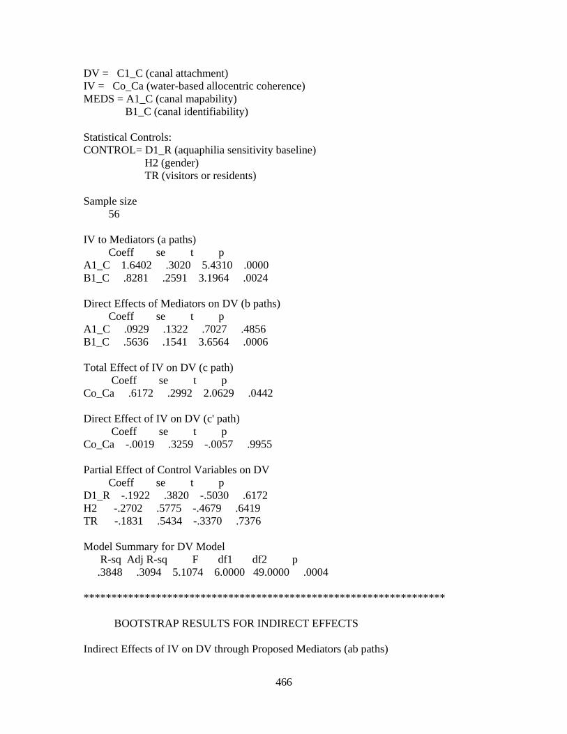
466
DV = C1_C (canal attachment)
IV = Co_Ca (water-based allocentric coherence)
MEDS = A1_C (canal mapability)
B1_C (canal identifiability)
Statistical Controls:
CONTROL= D1_R (aquaphilia sensitivity baseline)
H2 (gender)
TR (visitors or residents)
Sample size
56
IV to Mediators (a paths)
Coeff se t p
A1_C 1.6402 .3020 5.4310 .0000
B1_C .8281 .2591 3.1964 .0024
Direct Effects of Mediators on DV (b paths)
Coeff se t p
A1_C .0929 .1322 .7027 .4856
B1_C .5636 .1541 3.6564 .0006
Total Effect of IV on DV (c path)
Coeff se t p
Co_Ca .6172 .2992 2.0629 .0442
Direct Effect of IV on DV (c' path)
Coeff se t p
Co_Ca -.0019 .3259 -.0057 .9955
Partial Effect of Control Variables on DV
Coeff se t p
D1_R -.1922 .3820 -.5030 .6172
H2 -.2702 .5775 -.4679 .6419
TR -.1831 .5434 -.3370 .7376
Model Summary for DV Model
R-sq Adj R-sq F df1 df2 p
.3848 .3094 5.1074 6.0000 49.0000 .0004
*****************************************************************
BOOTSTRAP RESULTS FOR INDIRECT EFFECTS
Indirect Effects of IV on DV through Proposed Mediators (ab paths)

467
Data Boot Bias SE
TOTAL .6190 .6253 .0063 .2000
A1_C .1524 .1672 .0149 .2190
B1_C .4667 .4580 -.0086 .1880
Bias Corrected Confidence Intervals
Lower Upper
TOTAL .2489 1.0663
A1_C -.1904 .6858
B1_C .1605 1.0056
*****************************************************************
Level of Confidence for Confidence Intervals:
95
Number of Bootstrap Resamples:
1000
********************************* NOTES********************************
------ END MATRIX -----
Model O
Dependent, Independent, and Proposed Mediator Variables:
DV = C1_C (canal attachment)
IV = Co_Ce (water-based egocentric coherence)
MEDS = A1_C (canal mappability)
Statistical Controls:
CONTROL= D1_R (aquaphilia sensitivity baseline)
H2 (gender)
TR (visitors or residents)
Sample size
51
IV to Mediators (a paths)
Coeff se t p
A1_C 1.8909 .4754 3.9772 .0002
Direct Effects of Mediators on DV (b paths)
Coeff se t p
A1_C .2822 .1222 2.3095 .0256
Total Effect of IV on DV (c path)
Coeff se t p

468
Co_Ce 1.0404 .4122 2.5241 .0151
Direct Effect of IV on DV (c' path)
Coeff se t p
Co_Ce .5068 .4568 1.1094 .2731
Partial Effect of Control Variables on DV
Coeff se t p
D1_R .0581 .4144 .1401 .8892
H2 -.8589 .6402 -1.3416 .1865
TR -.3760 .5974 -.6294 .5323
Model Summary for DV Model
R-sq Adj R-sq F df1 df2 p
.2879 .2087 3.6381 5.0000 45.0000 .0075
*****************************************************************
BOOTSTRAP RESULTS FOR INDIRECT EFFECTS
Indirect Effects of IV on DV through Proposed Mediators (ab paths)
Data Boot Bias SE
TOTAL .5336 .5495 .0158 .3312
A1_C .5336 .5495 .0158 .3312
Bias Corrected Confidence Intervals
Lower Upper
TOTAL .0858 1.4636
A1_C .0858 1.4636
*****************************************************************
Level of Confidence for Confidence Intervals:
95
Number of Bootstrap Resamples:
1000
********************************* NOTES********************************
------ END MATRIX -----
Model O1
Dependent, Independent, and Proposed Mediator Variables:
DV = C1_C (canal attachment)
IV = Co_Ce (water-based egocentric coherence)
MEDS = B1_C (canal identifiability)

469
Statistical Controls:
CONTROL= D1_R (aquaphilia sensitivity baseline)
H2 (gender)
TR (visitors or residents)
Sample size
51
IV to Mediators (a paths)
Coeff se t p
B1_C .6558 .4029 1.6276 .1104
Direct Effects of Mediators on DV (b paths)
Coeff se t p
B1_C .5362 .1299 4.1289 .0002
Total Effect of IV on DV (c path)
Coeff se t p
Co_Ce 1.0404 .4122 2.5241 .0151
Direct Effect of IV on DV (c' path)
Coeff se t p
Co_Ce .6888 .3650 1.8872 .0656
Partial Effect of Control Variables on DV
Coeff se t p
D1_R .0654 .3645 .1795 .8583
H2 -.4254 .5915 -.7193 .4757
TR .2952 .5079 .5811 .5641
Model Summary for DV Model
R-sq Adj R-sq F df1 df2 p
.4223 .3581 6.5793 5.0000 45.0000 .0001
*****************************************************************
BOOTSTRAP RESULTS FOR INDIRECT EFFECTS
Indirect Effects of IV on DV through Proposed Mediators (ab paths)
Data Boot Bias SE
TOTAL .3516 .3774 .0257 .2609
B1_C .3516 .3774 .0257 .2609
Bias Corrected Confidence Intervals
Lower Upper

470
TOTAL -.0642 1.0020
B1_C -.0642 1.0020
*****************************************************************
Level of Confidence for Confidence Intervals:
95
Number of Bootstrap Resamples:
1000
********************************* NOTES********************************
------ END MATRIX -----
Model O2
Dependent, Independent, and Proposed Mediator Variables:
DV = C1_C (canal attachment)
IV = Co_Ce (water-based egocentric coherence)
MEDS = A1_C (canal mappability)
B1_C (canal identifiability)
Statistical Controls:
CONTROL= D1_R (aquaphilia sensitivity baseline)
H2 (gender)
TR (visitors or residents)
Sample size
51
IV to Mediators (a paths)
Coeff se t p
A1_C 1.8909 .4754 3.9772 .0002
B1_C .6558 .4029 1.6276 .1104
Direct Effects of Mediators on DV (b paths)
Coeff se t p
A1_C .0431 .1337 .3227 .7484
B1_C .5079 .1577 3.2200 .0024
Total Effect of IV on DV (c path)
Coeff se t p
Co_Ce 1.0404 .4122 2.5241 .0151
Direct Effect of IV on DV (c' path)
Coeff se t p
Co_Ce .6257 .4172 1.4998 .1408

471
Partial Effect of Control Variables on DV
Coeff se t p
D1_R .0391 .3771 .1036 .9180
H2 -.4289 .5975 -.7178 .4767
TR .2125 .5734 .3707 .7127
Model Summary for DV Model
R-sq Adj R-sq F df1 df2 p
.4237 .3451 5.3910 6.0000 44.0000 .0003
*****************************************************************
BOOTSTRAP RESULTS FOR INDIRECT EFFECTS
Indirect Effects of IV on DV through Proposed Mediators (ab paths)
Data Boot Bias SE
TOTAL .4147 .4433 .0286 .3699
A1_C .0816 .1053 .0238 .2912
B1_C .3331 .3380 .0049 .2672
Bias Corrected Confidence Intervals
Lower Upper
TOTAL -.1381 1.3499
A1_C -.4680 .7368
B1_C -.0158 1.1258
*****************************************************************
Level of Confidence for Confidence Intervals:
95
Number of Bootstrap Resamples:
1000
********************************* NOTES********************************

472
REFERENCES CITED
Chapter I
Adger, W. N., Hughes, T. P., Folke, C., Carpenter, S. R., & Rockström, J. (2005). Social-
ecological resilience to coastal disasters. science, 309(5737), 1036-1039.
Appleyard, D. (1976). Planning a pluralist city: Conflicting realities in Ciudad Guayana.
Beatley, T., & Newman, P. (2013). Biophilic cities are sustainable, resilient cities.
Sustainability, 5(8), 3328-3345.
Benedict, M. A., & McMahon, E. T. (2006). Green infrastructure. Island, Washington,
DC.
Black, R., Adger, W., Arnell, N., Dercon, S., Geddes, A., & Thomas, D. (2011). The
effect of environmental change on human migration. Global Environmental
Change, 21, S3-S11.
Black, R., Bennett, S., Thomas, S., & Beddington, J. (2011). Climate change: Migration
as adaptation. Nature, 478(7370), 447-449.
Brown, L. A., & Moore, E. G. (1970). The intra-urban migration process: a perspective.
Geografiska Annaler. Series B, Human Geography, 52(1), 1-13.
Burke, E. (1998). A philosophical enquiry into the sublime and beautiful: Penguin UK.
Cohen, N. (2000). Business location decision-making and the cities: bringing companies
back: Brookings Institution Center on Urban and Metropolitan Policy.
Corner, J. (2012). Terra fluxus. Lotus International, 150, 54-63.
Cosgrove, D., & Jackson, P. (1987). New directions in cultural geography. Area, 95-101.
Coss, R. G. (1990). All that glistens: Water connotations in surface finishes. Ecological
Psychology, 2(4), 367-380.
Deller, S. C., Tsai, T.-H. S., Marcouiller, D. W., & English, D. B. (2001). The role of
amenities and quality of life in rural economic growth. American Journal of
Agricultural Economics, 83(2), 352-365.
Doran, S., & Cannon, D. (2006). Cost-benefit analysis of urban stormwater retrofits and
stream daylighting using low impact development technologies. Proceedings of
the Water Environment Federation, 2006(9), 3833-3837.

473
Epstein, R. A., & Vass, L. K. (2014). Neural systems for landmark-based wayfinding in
humans. Philosophical Transactions of the Royal Society B: Biological Sciences,
369(1635), 20120533.
Fabricant, C. (1979). Binding and dressing nature's loose tresses: the Ideology of
Augustan landscape design.
Frediani, A. A., & Boano, C. (2012). Processes for just products: the capability space of
participatory design The Capability Approach, Technology and Design (pp. 203-
222): Springer.
Frenkel, S. (1994). Old Theories in New Places? Environmental Determinism and
Bioregionalism*. The Professional Geographer, 46(3), 289-295.
Gordon, D. (2002). New Urbanism and Smart Growth: Twins Separated at Birth?
PLACES-MASSACHUSETTS-, 15(2), 68-70.
Graham, S., & Healey, P. (1999). Relational concepts of space and place: issues for
planning theory and practice. European planning studies, 7(5), 623-646.
Hampton, E. (2002). Early settlement forms in America: recasting the framework of
foundations.
Hartmann, T. (2009). Clumsy floodplains and the law: towards a responsive land policy
for extreme floods. Built Environment, 35(4), 531-544.
Hirt, S. (2012). Jane Jacobs, Urban Visionary1. The Urban Wisdom of Jane Jacobs, 1.
Hooimeijer, F. (2011). The tradition of making: polder cities.
Howe, J., McMahon, E. T., & Propst, L. (2012). Balancing nature and commerce in
gateway communities: Island Press.
Huxtable, A. L. (1973). How We See or Think We See the City. The New York Timesi
Issue, Date, 26.
Kambites, C., & Owen, S. (2006). Renewed prospects for green infrastructure planning in
the UK 1. Planning, Practice & Research, 21(4), 483-496.
Karvonen, A. (2011). Politics of urban runoff: nature, technology, and the sustainable
city: MIT Press.
Korpela, K. M. (1989). Place-identity as a product of environmental self-regulation.
Journal of Environmental Psychology, 9(3), 241-256.
Laczko, F., & Aghazarm, C. (2009). Migration, environment and climate change:
Assessing the evidence: International Organization for Migration Geneva.

474
Lah, T. (2011). The huge success of the Cheonggyecheon restoration project: what’s left?
In M. K. Holzer, D; Bromberg, D. (Ed.), Citizen Participation: Innovative and
Alternative Modes for Engaging Citizens (pp. 97-118). Newark, NJ: National
Center for Public Performance.
Lewicka, M. (2011). Place attachment: How far have we come in the last 40 years?
Journal of Environmental Psychology, 31(3), 207-230. doi:
10.1016/j.jenvp.2010.10.001
Lynch, K. (1960). The Image of the City (pp. 91-117). Cambridge, MA: MIT Press.
Marcouiller, D. W., Kim, K.-K., & Deller, S. C. (2004). Natural amenities, tourism and
income distribution. Annals of Tourism Research, 31(4), 1031-1050.
Marcus, C. C., & Francis, C. (1997). People places: design guidlines for urban open
space: Wiley.
Marcus, C. C., & Sarkissian, W. (1988). Housing as if people mattered: Site design
guidelines for the planning of medium-density family housing (Vol. 4): University
of California Press.
Maslow, A. H., & Lewis, K. J. (1987). Maslow's hierarchy of needs: Salenger
Incorporated.
Mitchell, T. R. (1974). Cognitions and Skinner: Some questions about behavioral
determinism: University of Washington, School of Business Administration.
Moore, G. T., & Golledge, R. G. (1976). Environmental knowing: Theories, research and
methods: Dowden.
Newman, O. (1972). Defensible space: Crime prevention through urban design. New
York.
Nord, M., & Cromartie, J. (1997). Graphically Speaking: Migration: The increasing
importance of rural natural amenities. Choices, 12(3).
Pelton, T. (2005). Drug traces found in water pose problem for wildlife. Baltimore Sun.
Penning-Rowsell, E., Sultana, S., & Thompson, P. (2011). Population Movement in
Response to Climate Related Hazards in Bangladesh: The ‘Last Resort’.
Platteau, J. P. (2008). Pitfalls of participatory Development. Participatory Governance
and the Millennium Development Goals (MDGs), 127-162.
Quaiser-Pohl, C., Lehmann, W., & Eid, M. (2004). The relationship between spatial
abilities and representations of large-scale space in children—a structural
equation modeling analysis. Personality and Individual Differences, 36(1), 95-
107.
475
Rapoport, A. (1977). Human Aspect and Urban Form. New York: Pergarnon.
Raynsford, A. (2011). Civic art in an age of cultural relativism: the aesthetic origins of
Kevin Lynch's Image of the City. Journal of Urban Design, 16(1), 43-65.
Ruggeri, D. (2014). The ‘My Mission Viejo’Project. Investigating the Potential of
Photovoice Methods in Place Identity and Attachment Research. Journal of
Urban Design, 19(1), 119-139.
Savvas, D. (2003). Hydroponics: A modern technology supporting the application of
integrated crop management in greenhouse. JOURNAL OF FOOD
AGRICULTURE AND ENVIRONMENT, 1, 80-86.
Schensul, J. J., & LeCompte, M. D. (1999). Ethnographer's toolkit. Walnut Creek: CA:
AltaMira Press.
Shafer, S., Scott, D., Baker, J., & Winemiller, K. (2013). Recreation and amenity values
of urban stream corridors: implications for green infrastructure. Journal of Urban
Design, 18(4), 478-493.
Talen, E., & Duany, A. (2013). Landscape Urbanism and its Discontents Dissimulating
the Sustainable City. New York: New Society Publishers.
Tuan, Y.-F. (1974). Topophilia and Environment. Topophilia. A Study of Environmental
Perception, Attitudes and Values, 92-112.
Tzoulas, K., Korpela, K., Venn, S., Yli-Pelkonen, V., Kaźmierczak, A., Niemela, J., &
James, P. (2007). Promoting ecosystem and human health in urban areas using
Green Infrastructure: A literature review. Landscape and Urban Planning, 81(3),
167-178.
Ulrich, R. (1993). Biophilia, biophobia, and natural landscapes. In E. O. W. E. S.R.
Kellert (Ed.), The biophilia hypothesis (pp. 73-137). Washington, D.C.: Island
Press/Shearwater Books.
Vischer, J. (2001). Post-Occupancy Evaluation: a multifaceted tool for building
improvement. Learning from our buildings: a state-of-the-practice summary of
post-occupancy evaluation, 23-34.
Whyte, W. H. (1980). The Social Life of Small Urban Spaces.
Wilson, E. (1984). Biophilia: Harvard University Press.
Wilson, E. (1993). Biophilia and the conservation ethic. SR Kellert & E. 0. Wilson (Eds.),
The biophilia hypothesis, 2-41.

476
Zukin, S. (2007). Reading The Urban Villagers as a cultural document: Ethnicity,
modernity, and capital. City & Community, 6(1), 39-48.
Chapter II
Appleton, J. (1975). The Experience of Landscape. London: Wiley.
Backhaus, A., & Fryd, O. (2013). The esthetic performance of urban landscape-based
stormwater management systems: a review of twenty projects in Northern Europe.
Journal of Landscape Architecture, 8(2), 52-63.
Beardsley, M. C. (1958). Aesthetics. New York: Harcourt, Brace.
Beatley, T., & Newman, P. (2013). Biophilic cities are sustainable, resilient cities.
Sustainability, 5(8), 3328-3345.
Berlyne, D. E. (1974). Studies in the New Experimental Aesthetics: Steps toward an
Objective Psychology of Aesthetic Appreciation. New York: Halsted Press.
Coombes, P. J., Argue, J. R., & Kuczera, G. (2000). Figtree Place: a case study in water
sensitive urban development (WSUD). Urban Water, 1(4), 335-343.
Cullen, G. (1971). The Concise Townscape. New York: Reinhold.
Dosen, A. S., & Ostwald, M. J. (2013). Prospect and refuge theory: constructing a critical
definition for architecture and design. The International Journal of Design in
Society, 6(1), 9-24.
Ewing, R., Handy, S., Brownson, R. C., Clemente, O., & Winston, E. (2006). Identifying
and measuring urban design qualities related to walkability. Journal of Physical
Activity & Health, 3, S223.
Fisher-Gewirtzman, D., & Wagner, I. A. (2003). Spatial openness as a practical metric
for evaluating built-up environments. Environment and Planning B, 30(1), 37-50.
Golledge, R. (1984). An anchor point theory of the acquisition of spatial knowledge and
some empirical observations. Paper presented at the The Annual Meeting of the
Association of American Geographers.
Isaacs, R. (2000). The urban picturesque: an aesthetic experience of urban pedestrian
places. Journal of Urban Design, 5(2), 145-180.
Lennon, M., Scott, M., & O'Neill, E. (2014). Urban design and adapting to flood risk: the
role of green infrastructure. Journal of Urban Design, 19(5), 745-758.

477
Lynch, K. (1960). The Image of the City (pp. 91-117). Cambridge, MA: MIT Press.
Lynch, K. (1990). Notes on city satisfactions. In T. Banerjee & M. Southworth (Eds.),
City Sense and City Design (pp. 135-153). Cambridge, MA: MIT Press.
Mansor, M., & Said, I. (2008). Place attachment of residents to green infrastructure
network in small towns. Proceedings of the 9th SENVAR, 325-340.
Marquardt, G., & Schmieg, P. (2009). Dementia-friendly architecture: environments that
facilitate wayfinding in nursing homes. American journal of Alzheimer's disease
and other dementias, 24(4), 333-340.
Marsalek, J., & Chocat, B. (2002). International report: stormwater management. Water
Science & Technology, 46(6-7), 1-17.
Park, D. C., Puglisi, J. T., & Lutz, R. (1982). Spatial memory in older adults: effects of
intentionality. Journal of Gerontology, 37(3), 330-335.
Raynsford, A. (2011). Civic art in an age of cultural relativism: the aesthetic origins of
Kevin Lynch's Image of the City. Journal of Urban Design, 16(1), 43-65.
Shafer, S., Scott, D., Baker, J., & Winemiller, K. (2013). Recreation and amenity values
of urban stream corridors: implications for green infrastructure. Journal of Urban
Design, 18(4), 478-493.
Shannon, K., & Manawadu, S. (2007). Indigenous landscape urbanism: Sri Lanka's
reservoir & tank system. Journal of Landscape Architecture, 2(2), 6-17.
Sitte, C. (1945). The Art of Building Cities, trans. New York: Reinhold.
Unwin, R. (1908). Town and street planning. The Journal of the Royal Society for the
Promotion of Health, 29(9), 471-478.
Unwin, R. (1909). Town Planning in Practice: An Introduction to the Art of Designing
Cities and Suburbs. London: T. Fisher Unwin.
Unwin, R. (1914). Roads and Streets:" Illustrated". Town Planning Review, 5(1), 31.
Yu, K., Lei, Z., & Dihua, L. (2008). Living with water: flood adaptive landscapes in the
Yellow River basin of China. Journal of Landscape Architecture, 3(2), 6-17. doi:
10.1080/18626033.2008.9723400

478
Chapter III
Anderson, J., & Tindall, M. (1972). The concept of home range: New data for the study
of territorial behavior. Environmental design: Research and practice, 1, 1-7.
Appleyard, D. (1970). Styles and methods of structuring a city. Environment and
behavior.
Appleyard, D. (1976). Planning a pluralist city: Conflicting realities in Ciudad Guayana.
Baumgartner, T. A., & Chung, H. (2001). Confidence limits for intraclass reliability
coefficients. Measurement in Physical Education and Exercise Science, 5(3), 179-
188.
Beck, R. J., & Wood, D. (1976). Cognitive transformation of information from urban
geographic fields to mental maps. Environment and behavior, 8(2), 199-238.
Blades, M. (1990). The reliability of data collected from sketch maps. Journal of
Environmental Psychology, 10(4), 327-339.
Cackowski, J. M., & Nasar, J. L. (2003). The restorative effects of roadside vegetation
implications for automobile driver anger and frustration. Environment and
behavior, 35(6), 736-751.
Cicchetti, D. V. (1994). Guidelines, criteria, and rules of thumb for evaluating normed
and standardized assessment instruments in psychology. Psychological
assessment, 6(4), 284.
Coss, R. G. (1990). All that glistens: Water connotations in surface finishes. Ecological
Psychology, 2(4), 367-380.
Cronbach, L. J. (1951). Coefficient alpha and the internal structure of tests.
psychometrika, 16(3), 297-334.
De Jonge, D. (1962). Images of Urban Areas Their Structure and Psychological
Foundations. Journal of the American Institute of Planners, 28(4), 266-276.
Devlin, A. S. (1976). The “small town” cognitive map: Adjusting to a new environment.
Environmental Knowing: Theories, Research and Methods. Dowden, Hutchinson
and Ross.
Devlin, A. S., & Bernstein, J. (1995). Interactive wayfinding: Use of cues by men and
women. Journal of Environmental Psychology, 15(1), 23-38.
Evans, G. W. (1980). Environmental cognition. Psychological bulletin, 88(2), 259.

479
Ferguson, E. L., & Hegarty, M. (1994). Properties of cognitive maps constructed from
texts. Memory & cognition, 22(4), 455-473.
Gillner, S., & Mallot, H. A. (1998). Navigation and acquisition of spatial knowledge in a
virtual maze. Journal of Cognitive Neuroscience, 10(4), 445-463.
Golledge, R. G. (1992). Place recognition and wayfinding: Making sense of space.
Geoforum, 23(2), 199-214.
Golledge, R. G., & Stimson, R. (1997). Spatial behaviour: A geographic perspective.
Guilford, London.
Hallgren, K. A. (2012). Computing inter-rater reliability for observational data: An
overview and tutorial. Tutorials in quantitative methods for psychology, 8(1), 23.
Hume, C., Ball, K., & Salmon, J. (2006). Development and reliability of a self-report
questionnaire to examine children's perceptions of the physical activity
environment at home and in the neighbourhood. International Journal of
Behavioral Nutrition and Physical Activity, 3(1), 16.
Kaplan, S. (1976). Adaptation, structure and knowledge. In G. T. Moore & R. G.
Golledge (Eds.), Environmental knowing (pp. 32-45).
Kim, Y. O., & Penn, A. (2004). Linking the spatial syntax of cognitive maps to the
spatial syntax of the environment. Environment and behavior, 36(4), 483-504.
Kirasic, K. C., Allen, G. L., & Siegel, A. W. (1984). Expression of Configurational
Knowledge of Large-Scale Environments Students' Performance of Cognitive
Tasks. Environment and behavior, 16(6), 687-712.
Kreimer, A. (1973). Building the imagery of san francisco. An analysis of controversy
over high-rise development, 1970-71. Environmental Design Research, 2, 221-
231.
Kuipers, B. (1978). Modeling Spatial Knowledge*. Cognitive science, 2(2), 129-153.
Kwadijk, J. C., Haasnoot, M., Mulder, J. P., Hoogvliet, M., Jeuken, A., van der Krogt, R.
A., . . . van Waveren, H. (2010). Using adaptation tipping points to prepare for
climate change and sea level rise: a case study in the Netherlands. Wiley
Interdisciplinary Reviews: Climate Change, 1(5), 729-740.
Lawton, C. A. (1994). Gender differences in way-finding strategies: Relationship to
spatial ability and spatial anxiety. Sex roles, 30(11-12), 765-779.
Lynch, K. (1960). The Image of the City (pp. 91-117). Cambridge, MA: MIT Press.

480
MacLean, R. (2011). Venice of the North. Retrieved 01/17, 2013, from
http://blog.goethe.de/meet-the-germans/archives/173-Venice-of-the-North.html
Maguire, E. A., Burke, T., Phillips, J., & Staunton, H. (1996). Topographical
disorientation following unilateral temporal lobe lesions in humans.
Neuropsychologia, 34(10), 993-1001.
Mansor, M., & Said, I. (2008). Place attachment of residents to green infrastructure
network in small towns. Proceedings of the 9th SENVAR, 325-340.
McGraw, K. O., & Wong, S. P. (1996). Forming inferences about some intraclass
correlation coefficients. Psychological methods, 1(1), 30.
Milgram, S. (1976). Psychological maps of Paris. Environmental psychology : people and
their physical settings, 104-124.
Montello, D. R. (1998). A new framework for understanding the acquisition of spatial
knowledge in large-scale environments. Spatial and temporal reasoning in
geographic information systems, 143-154.
Moore, G. T., & Golledge, R. G. (1976). Environmental knowing: Theories, research and
methods: Dowden.
Osmond, H. (1963). What's New in Psychiatric Research. Mind: psychiatry in general
practice, 275.
Ostroff, C., & Schmitt, N. (1993). Configurations of organizational effectiveness and
efficiency. Academy of management Journal, 36(6), 1345-1361.
Piaget, J., & Inhelder, B. (1967). The child’s conception of space (FJ Langdon & JL
Lunzer, Trans.). New York.
Quaiser-Pohl, C., Lehmann, W., & Eid, M. (2004). The relationship between spatial
abilities and representations of large-scale space in children—a structural
equation modeling analysis. Personality and Individual Differences, 36(1), 95-
107.
Raplee, P. (2010). Ghent, Belgium: attractions, tours, and even a time lord. Retrieved
01/16, 2013, from http://www.offbeattravel.com/ghent-belgium-tours-attractions-
activities.html
Rovine, M. J., & Weisman, G. D. (1989). Sketch-map variables as predictors of way-
finding performance. Journal of Environmental Psychology, 9(3), 217-232.

481
Siegel, A. W. (1981). externalization of cognitive maps by children and adults: in search
of ways to ask better questions. Spatial representation and behavior across the
life span: theory and application/edited by LS Liben, AH Patterson, N.
Newcombe.
Siegel, A. W., & White, S. H. (1975). The development of spatial representations of
large-scale environments. Advances in child development and behavior, 10, 9.
Southworth, M., Cranz, G., Lindsay, G., & Morhayim, L. (2012). People in the Design of
Urban Places. Journal of Urban Design, 17(4), 461-465.
Tao, Z., & Zhengnan, Z. (2013). Urban surface water system in coastal areas: A
comparative study between Almere and Tianjin Eco-city. Open Journal of
Ecology, 2013.
Chapter IV
Alkon, A. H., & Traugot, M. (2008). Place matters, but how? Rural identity,
environmental decision making, and the social construction of place. City &
Community, 7(2), 97-112.
Appleyard, D. (1970). Styles and methods of structuring a city. Environment and
behavior.
Beatley, T. (2005). Native to nowhere: Sustaining home and community in a global age:
Island Press.
Beckley, T. M. (2003). The relative importance of sociocultural and ecological factors in
attachment to place. United States Department of Agricultural Forest Service
General Technical Report PNW, 105-126.
Bolund, P., & Hunhammar, S. (1999). Ecosystem services in urban areas. Ecological
Economics, 29(2), 293-301. doi: http://dx.doi.org/10.1016/S0921-8009(99)00013-
0
Carlson, E. D., Engebretson, J., & Chamberlain, R. M. (2006). Photovoice as a social
process of critical consciousness. Qualitative Health Research, 16(6), 836-852.
Davenport, M. A., & Anderson, D. H. (2005). Getting from sense of place to place-based
management: An interpretive investigation of place meanings and perceptions of
landscape change. Society and Natural Resources, 18(7), 625-641.
Davenport, M. A., Baker, M. L., Leahy, J. E., & Anderson, D. H. (2010). Exploring
multiple place meanings at an Illinois State Park. Journal of Park and Recreation
Administration, 28(1).

482
De Jonge, D. (1962). Images of Urban Areas Their Structure and Psychological
Foundations. Journal of the American Institute of Planners, 28(4), 266-276.
Feldman, R. M. (1990). Settlement-identity psychological bonds with home places in a
mobile society. Environment and behavior, 22(2), 183-229.
Fried, M. (1984). The structure and significance of community satisfaction. Population
and Environment, 7(2), 61-86.
Gieryn, T. F. (2000). A space for place in sociology. Annual review of sociology, 463-
496.
Golledge, R. G. (1992). Place recognition and wayfinding: Making sense of space.
Geoforum, 23(2), 199-214.
Golledge, R. G., & Stimson, R. (1997). Spatial behaviour: A geographic perspective.
Guilford, London.
Greider, T., & Garkovich, L. (1994). Landscapes: The social construction of nature and
the environment. Rural sociology, 59(1), 1-24.
Gustafson, P. (2006). 2 Place Attachment and Mobility. Multiple dwelling and tourism:
Negotiating place, home and identity, 17.
Hammitt, W. E., Backlund, E. A., & Bixler, R. D. (2006). Place bonding for recreation
places: Conceptual and empirical development. Leisure studies, 25(1), 17-41.
Hidalgo, M. C., & Hernandez, B. (2001). Place attachment: Conceptual and empirical
questions. Journal of Environmental Psychology, 21(3), 273-281.
Isaacs, R. (2000). The urban picturesque: an aesthetic experience of urban pedestrian
places. Journal of Urban Design, 5(2), 145-180.
Jorgensen, B. S., & Stedman, R. C. (2001). Sense of place as an attitude: Lakeshore
owners attitudes toward their properties. Journal of Environmental Psychology,
21(3), 233-248.
Jorgensen, B. S., & Stedman, R. C. (2006). A comparative analysis of predictors of sense
of place dimensions: Attachment to, dependence on, and identification with
lakeshore properties. Journal of environmental management, 79(3), 316-327.
Kaplan, S. (1984). Affect and cognition in the context of home: The quest for intangibles.
Population and Environment, 7(2), 126-133.
Kellert, S. R. (1995). The biophilia hypothesis: Island Press.

483
Kyle, G., Graefe, A., & Manning, R. (2005). Testing the dimensionality of place
attachment in recreational settings. Environment and behavior, 37(2), 153-177.
Lewicka, M. (2011). Place attachment: How far have we come in the last 40 years?
Journal of Environmental Psychology, 31(3), 207-230. doi:
10.1016/j.jenvp.2010.10.001
Lorenz, L. S., & Kolb, B. (2009). Involving the public through participatory visual
research methods. Health Expectations, 12(3), 262-274.
Lynch, K. (1960). The Image of the City (pp. 91-117). Cambridge, MA: MIT Press.
MacLean, R. (2011). Venice of the North. Retrieved 01/17, 2013, from
http://blog.goethe.de/meet-the-germans/archives/173-Venice-of-the-North.html
Mansor, M., & Said, I. (2008). Place attachment of residents to green infrastructure
network in small towns. Proceedings of the 9th SENVAR, 325-340.
Marcus, C. C., & Sarkissian, W. (1988). Housing as if people mattered: Site design
guidelines for the planning of medium-density family housing (Vol. 4): University
of California Press.
Mayer, F. S., & Frantz, C. M. (2004). The connectedness to nature scale: A measure of
individuals’ feeling in community with nature. Journal of Environmental
Psychology, 24(4), 503-515.
Milgram, S. (1976). Psychological maps of Paris. Environmental psychology : people and
their physical settings, 104-124.
Ogunseitan, O. A. (2005). Topophilia and the quality of life. Environmental Health
Perspectives, 113(2), 143.
Osmond, H. (1963). What's New in Psychiatric Research. Mind: psychiatry in general
practice, 275.
Proshansky, H. M., Fabian, A. K., & Kaminoff, R. (1983). Place-identity: physical world
socialization of the self. Journal of Environmental Psychology.
Raplee, P. (2010). Ghent, Belgium: attractions, tours, and even a time lord. Retrieved
01/16, 2013, from http://www.offbeattravel.com/ghent-belgium-tours-attractions-
activities.html
Raymond, C. M., Brown, G., & Weber, D. (2010). The measurement of place attachment:
Personal, community, and environmental connections. Journal of Environmental
Psychology, 30(4), 422-434.

484
Relph, E. (1976). Place and placelessness (Vol. 67): Pion London.
Ruggeri, D. (2014). The ‘My Mission Viejo’Project. Investigating the Potential of
Photovoice Methods in Place Identity and Attachment Research. Journal of
Urban Design, 19(1), 119-139.
Scannell, L., & Gifford, R. (2010a). Defining place attachment: A tripartite organizing
framework. Journal of Environmental Psychology, 30(1), 1-10.
Scannell, L., & Gifford, R. (2010b). The relations between natural and civic place
attachment and pro-environmental behavior. Journal of Environmental
Psychology, 30(3), 289-297.
Sommer, R. (1974). Tight spaces: Hard architecture and how to humanize it: Prentice-
Hall Englewood Cliffs, NJ.
Southworth, M., Cranz, G., Lindsay, G., & Morhayim, L. (2012). People in the Design of
Urban Places. Journal of Urban Design, 17(4), 461-465.
Southworth, M., & Ruggeri, D. (2010). Place, Identity And The Global City. Urban
Design Companion. London: Routledge.
Stedman, R. C. (2002). Toward a social psychology of place predicting behavior from
place-based cognitions, attitude, and identity. Environment and behavior, 34(5),
561-581.
Stedman, R. C. (2003a). Is it really just a social construction?: The contribution of the
physical environment to sense of place. Society &Natural Resources, 16(8), 671-
685.
Stedman, R. C. (2003b). Sense of place and forest science: Toward a program of
quantitative research. Forest science, 49(6), 822-829.
Stokman, A. (2008). Water purificative landscapes–constructed ecologies and
contemporary urbanism. Paper presented at the Transforming with water.
Proceedings of the 45th World Congress of the International Federation of
Landscape Architects IFLA.
Stokowski, P. A. (2002). Languages of place and discourses of power: Constructing new
senses of place. Journal of Leisure Research, 34(4), 368.
Tuan, Y.-F. (1974). Topophilia and Environment. Topophilia. A Study of Environmental
Perception, Attitudes and Values, 92-112.
Tuan, Y.-F. (1977). Space and place: The perspective of experience: U of Minnesota
Press.

485
Ulrich, R. (1993). Biophilia, biophobia, and natural landscapes. In E. O. W. E. S.R.
Kellert (Ed.), The biophilia hypothesis (pp. 73-137). Washington, D.C.: Island
Press/Shearwater Books.
Williams, D. R., & Vaske, J. J. (2003). The measurement of place attachment: Validity
and generalizability of a psychometric approach. Forest science, 49(6), 830-840.
Williams, D. R., Watson, A. E., & Alessa, L. (2001). Social construction of Arctic
wilderness: Place meanings, value pluralism, and globalization: USDA Forest
Service Rocky Mountain Research Station, 2150 Centre Avenue Fort Collins CO
80526 USA.
Wilson, G., & Baldassare, M. (1996). Overall" Sense of Community" in a Suburban
Region The Effects of Localism, Privacy, and Urbanization. Environment and
behavior, 28(1), 27-43.
Chapter V
Beatley, T. (2009). Biophilic urbanism: Inviting nature back to our communities and into
our lives. Wm. & Mary Envtl. L. & Pol'y Rev., 34, 209.
Beatley, T. (2011). Biophilic cities: integrating nature into urban design and planning:
Island Press.
Beatley, T., & Newman, P. (2013). Biophilic cities are sustainable, resilient cities.
Sustainability, 5(8), 3328-3345.
Cackowski, J. M., & Nasar, J. L. (2003). The restorative effects of roadside vegetation
implications for automobile driver anger and frustration. Environment and
Behavior, 35(6), 736-751.
Cela-Conde, C. J., Ayala, F. J., Munar, E., Maestu, F., Nadal, M., Capo, M. A., . . .
Marty, G. (2009). Sex-related similarities and differences in the neural correlates
of beauty. Proc Natl Acad Sci U S A, 106(10), 3847-3852. doi:
10.1073/pnas.0900304106
Clayton, K., & Woodyard, M. (1981). The acquisition and utilization of spatial
knowledge. Cognition, social behavior, and the environment, 151-161.
Coss, R. G. (1990). All that glistens: Water connotations in surface finishes. Ecological
Psychology, 2(4), 367-380.
Davies‐Colley, R., & Smith, D. (2001). TURBIDITY SUSPENI) ED SEDIMENT, AND
WATER CLARITY: A REVIEW1: Wiley Online Library.

486
Deller, S. C., Tsai, T.-H. S., Marcouiller, D. W., & English, D. B. (2001). The role of
amenities and quality of life in rural economic growth. American Journal of
Agricultural Economics, 83(2), 352-365.
Downs, R., & Siegel, A. (1981). On mapping researchers mapping children mapping
space. Spatial representation and behavior across the life span: Theory and
application, 237-248.
El-Sharkawy, H. M. A. (1979). Territoriality: a model for architectural design. Graduate
School of Arts and Sciences, University of Pennsylvania.
Golledge, R. G. (1992). Place recognition and wayfinding: Making sense of space.
Geoforum, 23(2), 199-214.
Hart, R. A. (1981). Children's spatial representation of the landscape: Lessons and
questions from a field study. Spatial representation and behavior across the life
span: theory and application/edited by LS Liben, AH Patterson, N. Newcombe.
Hartmann, T. (2010). Reframing polyrational floodplains: Land policy for large areas for
temporary emergency retention. Nature and Culture, 5(1), 15-30.
Hume, C., Ball, K., & Salmon, J. (2006). Development and reliability of a self-report
questionnaire to examine children's perceptions of the physical activity
environment at home and in the neighbourhood. International Journal of
Behavioral Nutrition and Physical Activity, 3(1), 16.
Jolliffe, I. (2002). Principal component analysis: Wiley Online Library.
Kaiser, H. F. (1960). The application of electronic computers to factor analysis.
Educational and psychological measurement.
Kaplan, S. (1984). Affect and cognition in the context of home: The quest for intangibles.
Population and Environment, 7(2), 126-133.
Kaplan, S. (1995). The restorative benefits of nature: toward an integrative framework.
Journal of Environmental Psychology, 15(3), 169-182.
Kellert, S. R. (1995). The biophilia hypothesis: Island Press.
Kellert, S. R. (2012). Building for life: Designing and understanding the human-nature
connection: Island press.
Korpela, K. (1989). Place-identity as a product of environmental self-regulation. Journal
of Environmental Psychology, 9, 241-256.

487
LaRue, L. H. (1974). Defensible Space, by Oscar Newman. Washington and Lee Law
Review, 31(3), 809.
Lewis, D. (1976). Observations on route finding and spatial orientation among the
aboriginal peoples of the western desert region of central Australia. Oceania, 249-
282.
Lynch, K. (1960). The Image of the City (pp. 91-117). Cambridge, MA: MIT Press.
MacKinnon, D. P., Fairchild, A. J., & Fritz, M. S. (2007). Mediation analysis. Annual
review of psychology, 58, 593.
MacKinnon, D. P., Lockwood, C. M., Hoffman, J. M., West, S. G., & Sheets, V. (2002).
A comparison of methods to test mediation and other intervening variable effects.
Psychological methods, 7(1), 83.
MacLean, R. (2011). Venice of the North. Retrieved 01/17, 2013, from
http://blog.goethe.de/meet-the-germans/archives/173-Venice-of-the-North.html
Maslow, A. H., & Lewis, K. J. (1987). Maslow's hierarchy of needs: Salenger
Incorporated.
McGraw, K. O., & Wong, S. P. (1996). Forming inferences about some intraclass
correlation coefficients. Psychological methods, 1(1), 30.
Newman, O. (1972). Defensible space: Crime prevention through urban design. New
York.
Newman, O. (1973). Defensible space (Vol. 973): Architectural Press London.
Nicholls, R. J., & Cazenave, A. (2010). Sea-level rise and its impact on coastal zones.
science, 328(5985), 1517-1520.
Ogunseitan, O. A. (2005). Topophilia and the quality of life. Environmental Health
Perspectives, 113(2), 143.
Osmond, H. (1963). What's New in Psychiatric Research. Mind: psychiatry in general
practice, 275.
Preacher, K. J., & Hayes, A. F. (2008). Asymptotic and resampling strategies for
assessing and comparing indirect effects in multiple mediator models. Behavior
research methods, 40(3), 879-891.
Raplee, P. (2010). Ghent, Belgium: attractions, tours, and even a time lord. Retrieved
01/16, 2013, from http://www.offbeattravel.com/ghent-belgium-tours-attractions-
activities.html

488
Rasmussen, K. (1931). The Netsilik Eskimos: Social Life and Spiritual Culture: Report of
the Fifth Thule Expedition 1921-24: Nordisk forlag.
Sommer, R. (1967). Sociofugal space. The American Journal of Sociology, 72(6), 654-
660.
Southworth, M., Cranz, G., Lindsay, G., & Morhayim, L. (2012). People in the Design of
Urban Places. Journal of Urban Design, 17(4), 461-465.
Stedman, R. C., & Ingalls, M. (2013). Topophilia, biophilia and greening in the red zone.
Greening in the Red Zone: Disaster, Resilience, and Community Greening.
Tuan, Y.-F. (1974). Topophilia and Environment. Topophilia. A Study of Environmental
Perception, Attitudes and Values, 92-112.
Vischer, J. (2001). Post-Occupancy Evaluation: a multifaceted tool for building
improvement. Learning from our buildings: a state-of-the-practice summary of
post-occupancy evaluation, 23-34.
Williams, D. R., Patterson, M. E., Roggenbuck, J. W., & Watson, A. E. (1992). Beyond
the commodity metaphor: Examining emotional and symbolic attachment to
place. Leisure Sciences, 14(1), 29-46.
Williams, D. R., & Roggenbuck, J. W. (1989). Measuring place attachment: Some
preliminary results. Paper presented at the NRPA Symposium on Leisure
Research, San Antonio, TX.
Wilson, E. (1984). Biophilia: Harvard University Press.
Chapter VI
Appleyard, Donald. 1970. Styles and methods of structuring a city. Environment and
behavior.
Beardsley, Monroe C. 1958. Aesthetics. New York: Harcourt, Brace.
Clayton, Keith, and Mary Woodyard. 1981. The acquisition and utilization of spatial
knowledge. Cognition, social behavior, and the environment:151-161.
Downs, RM, and AW Siegel. 1981. On mapping researchers mapping children mapping
space. Spatial representation and behavior across the life span: Theory and
application:237-248.

489
Golledge, Reginald G, and Robert Stimson. 1997. Spatial behaviour: A geographic
perspective. Guilford, London.
Hart, Roger A. 1981. Children's spatial representation of the landscape: Lessons and
questions from a field study. Spatial representation and behavior across the life
span: theory and application/edited by LS Liben, AH Patterson, N. Newcombe.
Isaacs, Raymond. 2000. The urban picturesque: an aesthetic experience of urban
pedestrian places. Journal of Urban Design 5 (2):145-180.
Jorgensen, Bradley S, and Richard C Stedman. 2001. Sense of place as an attitude:
Lakeshore owners attitudes toward their properties. Journal of environmental
psychology 21 (3):233-248.
Kirasic, Kathleen C, Gary L Allen, and Alexander W Siegel. 1984. Expression of
Configurational Knowledge of Large-Scale Environments Students' Performance
of Cognitive Tasks. Environment and Behavior 16 (6):687-712.
Lewicka, Maria. 2011. Place attachment: How far have we come in the last 40 years?
Journal of Environmental Psychology 31 (3):207-230.
Lewis, David. 1976. Observations on route finding and spatial orientation among the
aboriginal peoples of the western desert region of central Australia. Oceania:249-
282.
Lynch, Kevin. 1960. The Image of the City. Cambridge, MA: MIT Press.
Repeated Author. 1990. Notes on city satisfactions. In City Sense and City Design, edited
by T. Banerjee and M. Southworth. Cambridge, MA: MIT Press.
Münzer, Stefan, Hubert D Zimmer, Maximilian Schwalm, Jörg Baus, and Ilhan Aslan.
2006. Computer-assisted navigation and the acquisition of route and survey
knowledge. Journal of environmental psychology 26 (4):300-308.
Ogunseitan, Oladele A. 2005. Topophilia and the quality of life. Environmental Health
Perspectives 113 (2):143.
Piaget, Jean, and Barbel Inhelder. 1967. The child’s conception of space (FJ Langdon &
JL Lunzer, Trans.). New York.
Raynsford, Anthony. 2011. Civic art in an age of cultural relativism: the aesthetic origins
of Kevin Lynch's Image of the City. Journal of Urban Design 16 (1):43-65.
Stedman, Richard C. 2003. Is it really just a social construction?: The contribution of the
physical environment to sense of place. Society &Natural Resources 16 (8):671-
685.

490
Thorndyke, Perry W, and Barbara Hayes-Roth. 1982. Differences in spatial knowledge
acquired from maps and navigation. Cognitive psychology 14 (4):560-589.
Williams, Daniel R, and Jerry J Vaske. 2003. The measurement of place attachment:
Validity and generalizability of a psychometric approach. Forest science 49
(6):830-840.
Appleyard, Donald. 1970. Styles and methods of structuring a city. Environment and
behavior.
Clayton, Keith, and Mary Woodyard. 1981. The acquisition and utilization of spatial
knowledge. Cognition, social behavior, and the environment:151-161.
Downs, RM, and AW Siegel. 1981. On mapping researchers mapping children mapping
space. Spatial representation and behavior across the life span: Theory and
application:237-248.
Golledge, Reginald G, and Robert Stimson. 1997. Spatial behaviour: A geographic
perspective. Guilford, London.
Hart, Roger A. 1981. Children's spatial representation of the landscape: Lessons and
questions from a field study. Spatial representation and behavior across the life
span: theory and application/edited by LS Liben, AH Patterson, N. Newcombe.
Jorgensen, Bradley S, and Richard C Stedman. 2001. Sense of place as an attitude:
Lakeshore owners attitudes toward their properties. Journal of environmental
psychology 21 (3):233-248.
Kirasic, Kathleen C, Gary L Allen, and Alexander W Siegel. 1984. Expression of
Configurational Knowledge of Large-Scale Environments Students' Performance
of Cognitive Tasks. Environment and Behavior 16 (6):687-712.
Lewicka, Maria. 2011. Place attachment: How far have we come in the last 40 years?
Journal of Environmental Psychology 31 (3):207-230.
Lewis, David. 1976. Observations on route finding and spatial orientation among the
aboriginal peoples of the western desert region of central Australia. Oceania:249-
282.
Lynch, Kevin. 1960. The Image of the City. Cambridge, MA: MIT Press.
Münzer, Stefan, Hubert D Zimmer, Maximilian Schwalm, Jörg Baus, and Ilhan Aslan.
2006. Computer-assisted navigation and the acquisition of route and survey
knowledge. Journal of environmental psychology 26 (4):300-308.

491
Ogunseitan, Oladele A. 2005. Topophilia and the quality of life. Environmental Health
Perspectives 113 (2):143.
Piaget, Jean, and Barbel Inhelder. 1967. The child’s conception of space (FJ Langdon &
JL Lunzer, Trans.). New York.
Stedman, Richard C. 2003. Is it really just a social construction?: The contribution of the
physical environment to sense of place. Society &Natural Resources 16 (8):671-
685.
Thorndyke, Perry W, and Barbara Hayes-Roth. 1982. Differences in spatial knowledge
acquired from maps and navigation. Cognitive psychology 14 (4):560-589.
Williams, Daniel R, and Jerry J Vaske. 2003. The measurement of place attachment:
Validity and generalizability of a psychometric approach. Forest science 49
(6):830-840.