water tank and numerical model studies of ﬂow over steep...

Boundary-Layer MeteorolDOI 10.1007/s10546-006-9100-6

O R I G I NA L PA P E R

Water tank and numerical model studies of flow oversteep smooth two-dimensional hills

J. B. R. Loureiro · D. V. Soares · J. L. A. FontouraRodrigues · F. T. Pinho · A. P. Silva Freire

Received: 28 June 2005 / Accepted: 20 May 2006© Springer Science+Business Media B.V. 2006

Abstract The present work investigates the role of different treatments of the lowerboundary condition on the numerical prediction of flows over two-dimensional,smooth, steep hills. Four different law of the wall formulations are tested when alarge recirculating region is formed on the lee side of the hill. Numerical implementa-tion of the near-wall functions was made through a finite elements code. The standardκ–ε model was used to close the averaged Navier–Stokes equations. Results are vali-dated through original data obtained in a water tank. Measurements resorted to laserDoppler anemometry. The experiment provide detailed data for the characterizationof the reverse flow in the region between the separation and the reattachment points,with emphasis on the near wall region. The experimental wall shear stress distributionis compared with the results provided by the different laws of the wall showing goodagreement. The numerical predictions are shown to vary markedly between differentformulations.

Keywords Hill · κ–ε model · Laser-Doppler anemometry · Law of the wall ·Separation · Wall shear stress.

J. B. R. Loureiro (B) · A. P. Silva FreireMechanical Engineering Program (COPPE/UFRJ),Federal University of Rio de Janeiro,C.P. 68503, 21945-970, Rio de Janeiro, Brazile-mail: [email protected]

D. V. Soares · J. L. A. Fontoura RodriguesDepartment of Mechanical Engineering, University of Brasilia,70910-900, Brasilia, Brazil

F. T. PinhoCentro de Estudos de Fenómenos de Transporte,Faculdade de Engenharia da Universidade do Porto,Rua Dr. Roberto Frias s/n, 4200-465, Porto, Portugal

F. T. PinhoUniversidade do Minho, Largo do Paço, 4704-553, Braga, Portugal

Boundary-Layer Meteorol

1 Introduction

Non-uniformities resulting from changes in the surface are ubiquitous in micromete-orology, particularly surface roughness and hills. Unfortunately, from a mathematicalpoint of view, both conditions are difficult to treat analytically. This fact is much aggra-vated by the plain realization that the two conditions often occur simultaneously innature.

In this work we discuss the second condition, flow over hills. By considering theflow over a homogeneous surface, we aim at analysing changes in surface propertiesprovoked by changes in surface elevation alone. In particular, we discuss the role ofdifferent treatments of the lower boundary condition on the numerical prediction offlow properties. This is an aspect of the numerical modelling of flow over a hill that hasalways been known to be deficient. Here, four different law-of-the-wall formulationsare applied to the steep hill problem: the classical logarithmic expression, and theformulations of Mellor (1966), of Nakayama and Koyama (1984) and of Cruz andSilva Freire (1998, 2002). As presented, these formulations were specially introducedfor the prediction of flows subject to strong adverse pressure gradients; additionally,in their original form, they were developed to describe flows over an aerodynami-cally smooth surface. Thus, they resort to the canonical two-layered boundary-layerstructure to describe the far upstream undisturbed flow so that the existence of aviscous layer scaled by ν/u∗ is considered (ν = fluid kinematic viscosity, u∗ = frictionvelocity).

New data from a water-channel experiment of separated, aerodynamically smooth,turbulent flow over a steep hill are presented herein with the particular purpose ofvalidating the numerically simulated data. The experiments include local measure-ments of the mean and turbulent quantities of the flow, and were made using laserDoppler anemometry. The two-dimensional hill was constructed with a Witch ofAgnesi shape having a maximum 18.6◦slope. A flow visualization study, not presentedhere, was also performed.

The occurrence of flow separation downstream of steep hills adds much complexityto the problem. In fact, when hills become steep enough to form large downstreamrecirculation regions, not only the flow in the separated region changes, but significantchanges occur in the whole flow field over the hill. Under such conditions, many ofthe classical theories based on perturbation techniques break down. Quantifying theonset and extent of separation is hence a necessary and fundamental step for thecharacterization of the velocity field.

Therefore, the prediction of turbulent flow over a steep hill naturally lends itselfto the use of non-linear models. That has, indeed, been the general trend over thelast 10 years. The natural increase in computer power, together with the developmentof a host of turbulence models, has witnessed a large increase on the number ofnon-linear numerical simulations of atmospheric flows. Typical numerical simulationshave included two-equation eddy-viscosity turbulence models, algebraic Reynoldsstress models, second-order closure models and large-eddy simulation. All simula-tions, however, irrespective of the type of closure scheme chosen, suffer with thespecification of the boundary conditions at the wall.

A common approach, then, is to use the logarithmic law-of-the-wall formulation.Unfortunately, the mechanisms present in flow separation are poorly understoodso that the classical logarithmic expressions normally used to describe the flow inthe near-wall region do not find their counterpart near the separation point and in


the reverse flow region. This fact clearly poses severe difficulties for a numericalsimulation of the flow field, since any selected turbulence model should be capable ofwell representing all turbulence features down to the wall.

The present work studies the effects that a two-dimensional, steep, smooth hill hason the properties of a neutrally stable boundary layer. The analysis makes a compari-son between numerical and experimental results, having its focus on two main points:(i) to assess the applicability of the four previously mentioned wall functions for thedescription of the near-wall flow, and, (ii) to provide detailed experimental data forthe characterization of the recirculating flow in the region between the separation andthe reattachment points, with emphasis on the near-wall region.

2 Law-of-the-wall formulations

We introduce the different law-of-the-wall formulations that will be used in the imple-mentation of the numerical simulations.

Since the main concern of this work is to carry out a numerical simulation of theflow over a steep hill, just the main parts of the original derivations will be presentedhere. We must warn the reader that some of the derivations are quite detailed, arecurring feature that has really prevented us from going into too much detail. Still,to ensure legibility of the paper, the most relevant equations will be presented here infull. For a complete account of the formulations, the reader is referred to the originalreferences.

2.1 The logarithmic law-of-wall formulation for a smooth wall

For turbulent flows over a smooth wall, Prandtl (1925) considered the existence of aregion adjacent to the wall in which the total shear stress is nearly constant. Bearing inmind that viscosity must play a role in finding local solutions, a simple scaling analysisfurnishes u∗ and ν/u∗ as the two relevant scaling parameters.

The analysis may follow either from dimensional arguments or by mixing-lengththeory. Here, the second route is taken. Then, for the turbulent part of the wall regionwe may write

∂τ+t

∂z+ = ∂

∂z+ (−u′+w′+) = ∂

∂z+

(�2z+2

(∂u+

∂z+

)2)

, (1)

where the notation is standard. The dash denotes a quantity fluctuation, u+ = u/u∗,τ+

t = τt/(ρu2∗), τt = −ρu′w′, u′+w′+ = u′w′/u2∗ and z+ = z/(ν/u∗).Upon two successive integrations, we have

u+ = �−1 ln z+ + A, (2)

the classical law of the wall for a smooth surface (� = 0.4, A = 5.0) and zero-pressuregradient flows.

The action of an arbitrary pressure rise in the inner layer will distort the velocityprofile until the pressure gradient is solely balanced by the gradient of shear stress.Near a separation point, Eq. (2) presents clear difficulties as u∗ → 0.


2.2 The law-of-the-wall formulation of Mellor (1966)

The effect of pressure gradients on the behaviour of turbulent boundary layers with-out restriction to equilibrium was investigated by Mellor (1966) through dimensionalarguments. When a large external pressure gradient is applied to a boundary layer,no portion of the defect profile overlaps the logarithmic law. In fact, as previouslysuggested by Coles (1956) and by Stratford (1959), very near a separation point thelogarithmic part of the velocity profile ceases to exist. However, if Millikan’s (1939)arguments are recast and a new pressure gradient parameter is included in the analy-sis, an equation can be derived that satisfies the required limiting form as a separationpoint is approached.

Making the approximation that in the viscous sublayer the stress terms should bebalanced only by the pressure term in the motion equations, Mellor (1966) found

u+ = z+ + 12 p+z+2, (3)

for the inner region of the boundary layer, whereas for the outer layer he wrote

u+ = ξp+ + 2�

(√1 + p+z+ − 1

)+ 1

�ln

(4z+

2 + p+z+ + 2√

1 + p+z+

), (4)

where z+ = zupν/ν, u+ = u/upν , upν = [(ν/ρ)(dp/dx)]1/3 and p+ = [(ν/ρ)(dp/dx)]/u3∗. Equation (4) follows different asymptotic behaviours in the limiting cases p+ →0 or ∞, tending respectively to the classical logarithmic law or to Stratford’s equation.Function ξp+ is a known parameter having been determined numerically for a rangeof p+ values (Table 1).

Equations (3) and (4) were specified for the viscous and logarithmic regions, respec-tively. For numerical purposes, these regions were considered to intersect at z+ = 11.64,which was considered to be the point of mathematical intersection of the viscous andlogarithmic regions for the classical law of the wall. Regarding the law-of-the-wallformulations that take into account the effects of adverse pressure gradients, themathematical intersection of the inner and logarithmic functions depends on thevalue of the dimensionless pressure p+.

2.3 The law-of-the-wall formulation of Nakayama and Koyama (1984)

Nakayama and Koyama (1984) obtained a law of the wall for boundary layers subjectto adverse pressure gradients by conducting a one-dimensional analysis on the tur-bulent kinetic energy equation with assumptions of local similarity. Considering thetwo possible limiting cases of a constant stress layer and of a zero wall-stress layer,the authors propose a turbulent kinetic energy equation that upon integration yields,

u+ = 1�+

[3(ζ − ζs) + ln

(ζs + 1ζs − 1

ζ − 1ζ + 1

)], (5)

Table 1 Integration function (Mellor, 1966), p+

p+ −0.01 0.00 0.02 0.05 0.1 0.2 0.5 1 2 10ξp+ 4.92 4.90 4.94 5.06 5.26 5.63 6.44 7.34 8.49 12.13


where

ζ =(1 + 2τ+

3

)1/2. (6)

The above formulation introduces a von Kármán modified constant, �+, and theslip value, ζs. For a boundary layer subject to an adverse pressure gradient,

τ+ = 1 + p+z+, (7a)

p+ = νρ1/2(dτ/dz)w/τ3/2w , (7b)

z+ = (τw/ρ)1/2z/ν. (7c)

The von Kármán modified constant was estimated to be

�+(p+) = 0.419 + 0.539p+

1 + p+ . (8)

The slip value ζs was determined from the condition that in the limiting case p+ → 0the above formulation reduces to the classical law of the wall, Eq. (2). It follows that

ζs(p+) = (1 + (2/3)e−�Ap+)1/2 ≈ (1 + 0.074p+)1/2. (9)

Nakayama and Koyama (1984) considered their analysis general in the sense thatvelocity was related to the local shear stress instead of to the distance from the wall.Additionally, the analysis does not have to be restricted to a linear velocity–stressrelation but can be applied for any monotonically increasing shear stress layer.

2.4 The law-of-the-wall formulation of Cruz and Silva Freire (1998, 2002)

Introducing a new scaling procedure, Cruz and Silva Freire (2002) proposed the lawof the wall for a separating flow to be written as

u = τw

|τw|2�

√τw

ρ+ 1

ρ

dPw

dxz + τw

|τw|u∗�

ln

(z

Lc

), (10)

where

Lc =

√(τwρ

)2 + 2 νρ

dPw

dxuR − τw

ρ

1ρ

dPwdx

, (11)

� = 0.4, u∗ is the friction velocity, and uR (=√τp/ρ, τp = total shear stress) is a

reference velocity.The total shear stress, τp, can be evaluated from

τp = C1/2µ ρκp + µ

∣∣∣∂u∂z

∣∣∣p, (12)

where the subscript p denotes an adequately chosen location, normally the first gridpoint in the computational domain, Cµ (= 0.09) is a constant of the κ–ε model and κ

is the turbulent kinetic energy.


Equation (12) was obtained from a momentum balance in the near-wall region;it is similar to a relation usually employed by other authors to relate the wall shearstress to the turbulent kinetic energy in a κ–ε formulation (see, e.g., Launder and Spal-ding (1974), the only difference here is the inclusion of the viscous term to improvecalculations when z/Lc ≤ 30).

To find a first estimate for the wall shear stress, τwo, Eqs. (2) and (12) can becombined to give

τwo = upC1/4µ τp

1/2ρ1/2�

ln(

E z (τp/ρ)1/2

ν

) , (13)

with E = e�A.The pressure gradient at the wall can be obtained through Eqs. (12) and (13),

dPw

dx= τp − τwo

zp, (14)

which results directly from the inner layer approximated equations, and representsthe balance of forces in that layer.

Next, the characteristic length can be calculated from

Lc =

√(τwoρ

)2 + 2 νρ

dPw

dxuR − τwo

ρ

1ρ

dPw

dx

. (15)

Finally, the wall shear stress is calculated from Eq. (10) according to

τw = upτp1/2ρ1/2�

2√∣∣∣ τp

τwo

∣∣∣ + ln( zp

Lc

) . (16)

Using some production–dissipation equilibrium assumptions and Eq. (10) thekinetic energy dissipation and the production terms can be written respectively asfollows:

Dissipation = Cµ

12 κp

((τp/ρ)1/2

�z+

1ρ

dPwdx

�(τp/ρ)1/2

), (17)

Production = Cµ

12 κpρ

z

(2(τp/ρ)

12

�+ | (τwo/ρ) | 1

2

�ln

(z

Lc

)). (18)

Equation (10) is a generalization of the classical law of the wall and replaces thethree expressions advanced in Cruz and Silva Freire (1998—their Eqs. (25), (26), (27)).Equation (11) is an expression for the near-wall region characteristic length, which isassumed to be valid in the attached and in the reverse flow regions.

Far away from the separation point, where the wall shear stress is positive andz(dPw/dx) << τw, Eq. (10) reduces to the classical law of the wall, Eq. (2),

u = 2�

u∗ + u∗�

ln

(z

Lc

), (19a)


Lc = ν/u∗. (19b)

Near to the separation point where τw = 0, Eq. (10) leads to

u = 2�

√zρ

dPw

dx, (20)

which is indeed Stratford’s equation (see Stratford 1959).In the reverse flow region where the wall shear stress is negative and z(dPw/dx) <<

τw, Eq. (10) reads

u = − 2�

u∗ − u∗�

ln

(z

Lc

), (21a)

Lc = 2∣∣∣ τw

dPw/dx

∣∣∣. (21b)

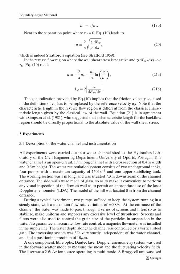
The generalization provided by Eq.(10) implies that the friction velocity, u∗, usedin the definition of Lc has to be replaced by the reference velocity uR. Note that thecharacteristic length in the reverse flow region is different from the classical charac-teristic length given by the classical law of the wall. Equation (21) is in agreementwith Simpson et al. (1981), who suggested that a characteristic length for the backflowregion should be directly proportional to the absolute value of the wall shear stress.

3 Experiments

3.1 Description of the water channel and instrumentation

All experiments were carried out in a water channel sited at the Hydraulics Lab-oratory of the Civil Engineering Department, University of Oporto, Portugal. Thiswater channel is an open-circuit, 17 m long channel with a cross-section of 0.4 m widthand 0.6 m height. The water recirculation system consists of two underground tanks,four pumps with a maximum capacity of 150 l s−1 and one upper stabilizing tank.The working section was 3 m long, and was situated 7.3 m downstream of the channelentrance. The side walls were made of glass, so as to make it convenient to performany visual inspection of the flow, as well as to permit an appropriate use of the laserDoppler anemometer (LDA). The model of the hill was located 8 m from the channelentrance.

During a typical experiment, two pumps sufficed to keep the system running in asteady state, with a maximum flow rate variation of ±0.8%. At the entrance of thechannel, the water was made to pass through a series of screens and filters so as tostabilize, make uniform and suppress any excessive level of turbulence. Screens andfilters were also used to control the grain size of the particles in suspension in thewater. To guarantee an accurate flow rate control, a magnetic flowmeter was installedin the supply line. The water depth along the channel was controlled by a vertical steelgate. The traversing system was 3D, very sturdy, independent of the water channel,and had a positioning precision of 10µm.

A one component, fibre optic, Dantec laser Doppler anemometry system was usedin the forward scatter mode to measure the mean and the fluctuating velocity fields.The laser was a 2 W Ar-ion source operating in multi-mode. A Bragg cell unit was used


to introduce an electronic shift of 0.6 MHz. This procedure allowed for the resolutionof the direction of the flow field and the correct measurement of near-zero meanvelocities. Front lenses of 310 mm focal length were mounted on the probe in order toaccurately position the measurement volume on the centreline of the channel. Beforebeing collected by the photomultiplier, the scattered light passed through an inter-ference filter of 514.5 nm, so that only green light was acquired. The signal from thephotomultiplier was band-pass filtered and processed by a TSI 1990C counter, oper-ating in single measurement per burst mode. A series of LDA biases were avoided byadjusting the strictest parameters on the data processor. For each point measured, asample size of 10,000 values has been considered. Mean and root-mean-square (rms)values of fluctuating quantities have been defined over this sample size according tothe Reynolds decomposition, which states that the instantaneous velocity equals thesum of a time-average component with a fluctuating component. The 10,000 samplesize was observed to be sufficient to ensure independent velocity results at each pointmeasured. Table 2 lists the main characteristics of the laser Doppler system used.

This system was used to measure both the longitudinal and the vertical velocitycomponents. This was easily made by simply turning the probe around its axis, so that,for both conditions, the fringe distribution was perpendicular to the measured velocitycomponent. As for the Reynolds shear stresses, measurements were made by turningthe probe to the positions ±45◦. For the undisturbed flow region, the uncertaintiesin the mean velocity components u and w are lower than 0.2% of the free streamvelocity, uδ . Further downstream of the hilltop, in high level turbulence regions, thesemaximum uncertainties increase to about 0.3% of the free stream velocity. As for the

fluctuating quantities,√

u′2,√

w′2, and u′w′, the estimated uncertainties in the undis-turbed flow region are of 2.3%, 1.8%, 4.2% of the friction velocity in the undisturbedflow (for the Reynolds shear stress the uncertainty is given as a percentage of thesquare of the friction velocity of the undisturbed flow), respectively, increasing to3.8%, 3.5% and 6.9% in regions of high turbulence.

3.2 Model hill characteristics

The model used in the present work was two-dimensional, axisymmetric and aero-dynamically smooth. Based on the works of Britter et al. (1981) and of Arya et al.(1987), the shape of the hill followed a modified “Witch of Agnesi” profile, accordingto the equation zH = H1[1 + (x/LH)2]−1 − H2. Thus, it follows that H (= H1 − H2)(= 60 mm) is the hill height and LH (= 150 mm) is the characteristic length of the hillrepresenting the distance from the crest to the half-height point. Co-ordinates x andz represent the longitudinal and the vertical axes, respectively.

Table 2 Main characteristics of the laser Doppler system

Wavelength 514.5 nmHalf-angle between beams 3.415◦Fringe spacing 4.3183 µmFrequency shift 0.60 MHz

Dimensions of the measurement volumeMajor axis 1.53 mmMinor axis 162.0 µm


Table 3 Hill features

Characteristic height H1 75 mmCharacteristic height H2 15 mmHill height H 60 mmHill length L 600 mmDistance from the crest to thehalf-height point LH 150 mmAspect ratio 2LH/H 5Maximum slope θmax 18.6◦

-15 -10 -5 0 10 15 20 25x/H

0

1

2

3

4

5

z/H

Separation(x/H = 0.5)

Reattachment(x/H = 6.67)

5

Fig. 1 Position of measuring stations and co-ordinate system

The geometry of the model was chosen so as to simulate a steep hill with a largerecirculation region, and the model was made of a single sheet of polished plexiglass.The characteristic parameters of hill are presented in Table 3.

When the hill was not in place, mean velocity results obtained in the x–z planes(see Fig. 1) located 50 mm away from the channel centreline to the right and to the leftshowed a variation of 2% in relation to measurements taken at the channel centreline.When the hill was in place, this value showed a variation of about 3%.

3.3 Experimental results

Results will be presented for the 13 stations indicated in Fig. 1 with the main purposeof serving as validation data for the numerical calculations to be introduced next. Tothat end, we will strive in furnishing mean velocity data. However, and since a detailedinvestigation of the turbulent properties was performed, some turbulent results willalso be presented. Please note the position of the co-ordinate system origin. Presen-tation of the data are split into three blocks: data for the flow field upstream of theseparation point (first three stations), data for the re-circulation region (next sevenstations) and data for the returning to equilibrium region (last three stations).

Results are mainly presented as plots with linear axes, as is normally the case.However, since in the comments below some mention will be made of the logarithmicbehaviour of the velocity field, four representative profiles are shown in log-linearcoordinates (Fig. 2d) so as to illustrate the referred behaviour.


0 0.4 0.8 1.2 1.6u/uδ

0

1

2

3

z/H

x/H = - 12.5x/H = -5x/H = -2.5x/H = 0

(a)

-0.4 0 0.4 0.8 1.2 1.6u/uδ

0

1

2

3

z/H

x/H = 0x/H = 0.5x/H = 1.25x/H = 2.5x/H = 3.75x/H = 5x/H = 6.67

(b)

0 0.4 0.8 1.2 1.6u/uδ

0

1

2

3

z/H

x/H = 6.67x/H = 10x/H = 15x/H = 20

(c)

-0.4 0 0.4 0.8 1.2 1.6u/uδ

-6

-4.5

-3

-1.5

0

1.5

3L

n (z

/H)

x/H = -12.5x/H = 0x/H = 3.75x/H = 20

(d)

Fig. 2 Mean velocity profiles, x-component (a–c). Four representative logarithmic profiles are shownin (d)

Figures 2 and 3 show the mean velocity profiles. The flow acceleration region onthe upstream side of hill is illustrated in Fig. 2a, and at stations x/H = −12.5, −5 and−2.5 the well-known law of the wall is very well discriminated. Figure 2d illustratesthe logarithmic velocity profile measured at x/H = −12.5. In all three profiles, at least11 points could be identified as belonging to the logarithmic region, yielding straightlines with coefficients of determination R2 higher than 0.99. In addition, seven extrapoints were observed to be located in the viscous region; von Kármán’s constant wasfound to be 0.39.

The local properties of the boundary layer in the undisturbed flow are shown inTable 4. The longitudinal and vertical fluctuations obtained in this experiments arerepresentative of atmospheric values. This fact can be inferred from a comparisonwith typical values of near-surface fluctuations in neutrally stratified flows. For exam-

ple, the following data are taken from the literature:√

u′2/u∗ = 2.3 and√

w′2/u∗ =1.1 (Grant 1992),

√u′2/u∗ = 2.12 (Britter et al. 1981),

√u′2/u∗ = 2.5 and

√w′2/u∗ =

1.2 (Khurshudyan et al. 1981),√

u′2/u∗ = 2.2 and√

w′2/u∗ = 1.0 (Gong and Ibbetson

1986) and√

u′2/u∗ = 2.19 and√

w′2/u∗ = 1.12 (Athanassiadou and Castro 2001).


0 0.1 0.2 0.3 0.4

w/uδ

0

1

2

3

z/H

x/H = - 12.5x/H = -5x/H = -2.5x/H = 0

(a)

-0.2 0 0.2 0.4

w/uδ

0

1

2

3

z/H

x/H = 0x/H = 0.5x/H = 1.25x/H = 2.5x/H = 3.75x/H = 5x/H = 6.67

(b)

-0.1 0 0.1 0.2

w/uδ

0

1

2

3

z/H

x/H = 6.67x/H = 10x/H = 15x/H = 20

(c)

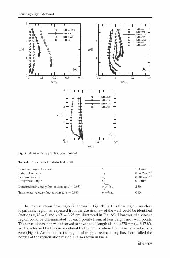
Fig. 3 Mean velocity profiles, z-component

Table 4 Properties of undisturbed profile

Boundary layer thickness δ 100 mmExternal velocity uδ 0.0482 m s−1

Friction velocity u∗ 0.0035 m s−1

Roughness length z0 0.27 mm

Longitudinal velocity fluctuations (z/δ = 0.05)√

u′2/u∗ 2.50

Transversal velocity fluctuations (z/δ = 0.08)√

w′2/u∗ 0.83

The reverse mean flow region is shown in Fig. 2b. In this flow region, no clearlogarithmic region, as expected from the classical law of the wall, could be identified(stations x/H = 0 and x/H = 3.75 are illustrated in Fig. 2d). However, the viscousregion could be discriminated for each profile from, at least, eight near-wall points.The separation region was observed to have a total length of about 370 mm (= 6.17 H),as characterized by the curve defined by the points where the mean flow velocity iszero (Fig. 4). An outline of the region of trapped recirculating flow, here called theborder of the recirculation region, is also shown in Fig. 4.


-4 -2 0

x/H

0.0

0.4

0.8

1.2

1.6

2.0

z/H

Locus U = 0Recirculation border

8642

Fig. 4 Locus of zero longitudinal velocity in the re-circulation region

The mean longitudinal velocity profiles downstream of the hill are presented inFig. 2c. Although much disturbed by the separation region, all four quoted profilespresented well-discriminated logarithmic regions. In fact, at least 12 points were usedto determine the logarithmic region through straight lines with coefficients of deter-mination, R2, higher than 0.99 (station x/H = 20 is shown in Fig. 2d).

The mean z-velocity profiles, w, show a large increase as the fluid flows uphill (Fig.3a), followed by negative values of velocity on the downside of the hill (Fig. 3b). Infact, due to the extension of the separation bubble that is formed, the mean z-velocityprofile only becomes negative past station x/H = 2.5. As station x/H = 10 is reached(Fig. 3c), w returns to a near-zero value.

The changes in Reynolds stresses are shown in Figs. 5–7, where measurementsindicate a decrease in u′2 on the upstream side of the hill, possibly due to the accel-erated mean flow (Fig. 5a). In particular, on the hill top, a slight decrease in u′2 isobserved. In the separated flow region (Fig. 5b), a substantial enhancement in u′2,of the order of four times, occurs. The large increase in u′2 results from the largeturbulence production provoked by Puu = −2u′w′(∂u/∂z). The peak value for u′2 wasfound for x/H = 3.75 and z/H = 0.8, near the centre of the recirculation bubble. Inthe flow separated region, the turbulence profiles are characterized by a maximumpeak progressively moving away from the wall with increasing distance from the hill.Far away from the hill, at stations x/H = 15 and 20, the two u′2 profiles are stilleasily distinguished from each other and different from the undisturbed profile atx/H = −12.5.

For w′2 an increase of about 50% is observed at the hilltop as compared to theundisturbed values. This increase is followed by a further, and much more substantial,increase of about twentyfold in the separated flow region. Indeed, we had seen previ-ously that a large increase in w was observed uphill. The role of this increase is, in itsturn, to increase the production of w′2 through Pww = −2u′w′(∂w/∂x).

The distributions of u′2 and of w′2 are somewhat similar across the separated region,although w′2 is about 65% of u′2. Indeed, the turbulence productionPuu = −2u′w′(∂u/∂z) is expected to exceed the term Pww = −2u′w′(∂w/∂x), since inthis region (∂u/∂z) > (∂w/∂x). Also, we note that the maximum value of w′2 is foundat x/H = 3.75, z/H = 0.8, just as before. Far away from the hill, at stations x/H = 15and 20, the two w′2 profiles are still very different from each other.

The Reynolds stress profile, −u′w′, is relatively small upwind of the hill and variesslowly with height. At the hill crest, values of −u′w′ are enhanced. In the shear layer


0 0.01 0.02 0.03

u'2/uδ2

0

1

2

3

z/H

x/H = -12.5x/H = -5x/H = -2.5x/H = 0

(a)

0 0.04 0.08 0.12

u'2/uδ2

0

1

2

3

z/H

x/H = 0x/H = 0.5x/H = 1.25x/H = 2.5x/H = 3.75x/H = 5x/H = 6.67

(b)

0 0.02 0.04 0.06 0.08

u'2/uδ2

0

1

2

3

z/H

x/H = 6.67x/H = 10x/H = 15x/H = 20

(c)

Fig. 5 Normalized Reynolds stress profiles, u′2/u2δ

that is formed at the top of the flow separated region, a large increase in −u′w′ isobserved, of the order of 17 times. This is due to the enhanced shear effects throughthe production term Puw=−2w′2(∂u/∂z). The highest value of −u′w′ is achieved atlocation x/H = 3.75, z/H = 0.6, differently from the positions of the points of maxi-mum for u′2 and for w′2. Between the locations of detachment and of re-attachment,an inner region of constant −u′w′ was not detected. Far downstream of the hill, atstations x/H = 15 and 20, −u′w′ becomes nearly constant.

To find the wall shear stress in regions where the flow is attached chart methodsbased on the logarithmic law may be used under some conditions. Additionally, theidentification of an existing constant shear-stress wall layer can also be used. In areverse flow region, however, some alternative technique has to be used to find thewall shear stress.

Consider that in a turbulent boundary layer the very near-wall region is dominatedby viscous effects. Then, under adverse pressure gradient conditions, the momentumequation in the viscous sublayer has approximate balance of the viscous and pressureterms. A double integration of this equation furnishes a second-degree polynomial


0 0.003 0.006 0.0090

1

2

3

z/H

x/H = -12.5x/H = -5x/H = -2.5x/H = 0

(a)

0 0.03 0.06 0.09w'2/uδ

2w'2/uδ2

0

1

2

3

z/H

x/H = 0x/H = 0.5x/H = 1.25x/H = 2.5x/H = 3.75x/H = 5x/H = 6.67

(b)

0 0.03 0.06 0.09w'2/uδ

2

0

1

2

3

z/H

x/H = 6.67

x/H = 10

x/H = 15

x/H = 20

(c)

Fig. 6 Normalized Reynolds stress profiles, w′2/u2δ

relationship between the velocity and the distance from the wall, as shown previouslyin non-dimensional form by Eq. (3). In dimensional form, Eq. (3) reads

u = 12µ

∂p∂x

z2 + τw

µz. (22)

The correct application of the above equation to the experimental data requiresthe specification of an adequate coordinate system. For flows over a flat wall, thex-coordinate can be aligned with the mean flow direction, resulting in a rectangularCartesian system where the momentum balance in the x-direction contains most ofthe dynamical information regarding the flow. For flows over curved surfaces, Finn-igan (1983) suggests the use of physical streamlined coordinates. These coordinatesare, however, difficult to use in separated flow regions.

Here, at least eight measurement points were located in the first 3 mm away fromthe wall. In our worst case scenario, the wall tangent corresponds to an angle ofabout 14◦ (station x/H = 1.25). Since sin(14◦) = 0.24, the corresponding streamwisevelocity displacement along the normal direction will occur over a maximum distance


-0.004 0 0.004 0.008

-u'w'/uδ2

0

1

2

3

z/H

x/H = -12.5x/H = -5x/H = -2.5x/H = 0

(a)

0 0.02 0.04 0.06

-u'w'/uδ2

0

1

2

3

z/H

x/H = 0

x/H = 0.5

x/H = 1.25

x/H = 2.5

x/H = 3.75

x/H = 5

x/H = 6.67

(b)

0 0.02 0.04 0.06-u'w'/uδ

2

0

1

2

3

z/H

x/H = 6.67

x/H = 10

x/H = 15

x/H = 20

(c)

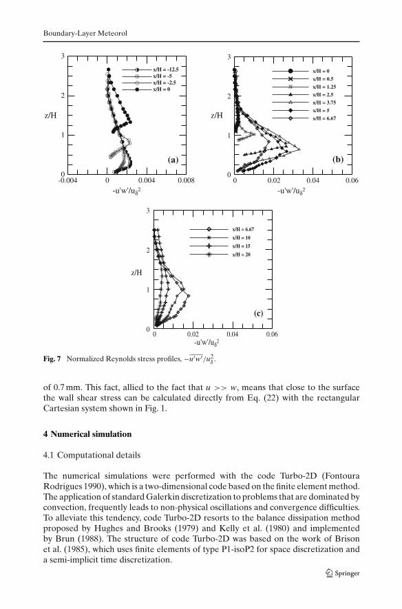
Fig. 7 Normalized Reynolds stress profiles, −u′w′/u2δ .

of 0.7 mm. This fact, allied to the fact that u >> w, means that close to the surfacethe wall shear stress can be calculated directly from Eq. (22) with the rectangularCartesian system shown in Fig. 1.

4 Numerical simulation

4.1 Computational details

The numerical simulations were performed with the code Turbo-2D (FontouraRodrigues 1990), which is a two-dimensional code based on the finite element method.The application of standard Galerkin discretization to problems that are dominated byconvection, frequently leads to non-physical oscillations and convergence difficulties.To alleviate this tendency, code Turbo-2D resorts to the balance dissipation methodproposed by Hughes and Brooks (1979) and Kelly et al. (1980) and implementedby Brun (1988). The structure of code Turbo-2D was based on the work of Brisonet al. (1985), which uses finite elements of type P1-isoP2 for space discretization anda semi-implicit time discretization.


The governing equations are the Reynolds averaged equations for an incompress-ible flow. Using the repeated indices convention, these equations can be written innon-dimensional form as

∂ui

∂xi= 0, (23)

∂ui

∂t+ ∂

∂xj(uiuj) = − ∂p

∂xi+ 1

Re

∂

∂xj

(∂ui

∂xj+ ∂uj

∂xi

)− ∂

∂xj

(u′

iu′j

), (24)

where ui represents the normalized velocity components, p the normalized pressureand Re the Reynolds number.

The Reynolds equations are complemented by the eddy viscosity formulation

− u′iu

′j = νt

(∂ui

∂xj+ ∂uj

∂xi

)− 2

3κδij, (25)

where νt denotes the eddy viscosity and δij is the Kronecker delta.In Eq. (25), κ is the turbulent kinetic energy,

κ = 12 u′

iu′i. (26)

In the κ–ε model, the eddy viscosity is taken to be

νt = Cµ

κ2

ε, (27)

where, Cµ(= 0.09) is a constant of the κ–ε model, and ε is the dissipation rate of κ .Equations for κ and for ε can be obtained directly from the Reynolds equations

through some algebraic manipulations. With further modelling, the resulting equa-tions can be cast as

∂κ

∂t+ ui

∂κ

∂xi= ∂

∂xi

[(1

Re+

(1

Rtσκ

))∂κ

∂xi

]+ Puiuj − ε, (28)

∂ε

∂t+ ui

∂ε

∂xi= ∂

∂xi

[(1

Re+

(1

Rtσε

))∂ε

∂xi

]+ Cε1

ε

κPuiuj − Cε2

ε2

κ, (29)

where Rt is the turbulent Reynolds number defined with the help of Eq. (27).Constants Cµ, Cε1, Cε2, σk and σε, as given in the literature, take values: 0.09, 1.44,

1.92, 1.0, 1.3. The production term, Puiuj , is given by

Puiuj = −u′iu

′j∂uj

∂xi. (30)

The governing equations are discretized in space through triangular finite elements,defined by linear interpolation functions. The compatibility conditions between pres-sure and velocity fields are preserved by using two calculation meshes. The pressurefield is calculated with a mesh with P1-type elements. Velocity and all other variablesare calculated using a P1-isoP2 mesh, constructed from the P1 mesh by dividing onesegment into two. This procedure generates four P1-isoP2 elements from one P1 ele-ment. Figure 8 shows the velocity and pressure meshes used to evaluate the flow fieldstudied in this work.


Fig. 8 Typical mesh distribution around the hill for pressure and velocity fields evaluation. (a) P1mesh with 1875 nodes and 3472 elements. (b) Iso/P2 mesh with 7221 nodes and 13888 elements

Table 5 Comparative computational times required to achieve numerical convergence for each ofthe law of the wall formulation considered

Formulation LogLaw M (1966) NK (1984) CSF (1998)Time 1 20 25 25

Temporal discretization of the governing equations is made through a sequentialsemi-implicit finite difference algorithm of Brison et al. (1985). The time iteration pro-cess was used to remove the influence of the initial conditions on the final calculations,so that simulation finishes only when statistically steady results have been reached. Infact, to keep a low sensitivity of the results to the time intervals, very fine timestepswould have to be used. Here, in order to optimize the convergence process, a temporalintegration procedure that progressively increased the timesteps was used. In a typicalsimulation, initial timesteps were about 10−6 s. This value was then increased steadilyto 5×10−2 s by the end of the simulation. These values were observed to ensure inde-pendence of results. For the velocity and pressure fields, and for the velocity boundaryconditions, the convergence criteria were set respectively to 10−8 and 10−6. Becausecomputational (cpu) times vary with local parameters (processor features, memorycapacity, grid refinement, convergence criteria), just comparative computational flowtimes are shown here (Table 5).

For code verification, Turbo-2D was tested against a number of data including thenumerical solution of Mansour et al. (1989) and the experimental data for flows over abackward facing step and in an asymmetric plane diffuser (Carlson et al. 1967; Reneauet al. 1967; Kim et al. 1980; Trupp et al. 1986; Buice and Eaton 1995).

A successful simulation of the flow under scrutiny depends, of course, on the correctspecification of the boundary conditions. Here, the inflow values of the mean velocity,of the turbulence kinetic energy and of the dissipation rate were taken directly fromthe experimental data. In the region adjacent to the surface, wall functions were usedas explained next. At the top, a free surface condition was used. For the outflow,symmetry (zero normal gradient) conditions were applied.


Since the standard κ–ε turbulence model does not hold for low values of the turbu-lent Reynolds number, a common practice is to use wall functions to express the flowbehaviour in the near-wall region, much as described in Sect. 3. In finite elements, themesh does not reach the wall. Thus, the velocity tangent to the solid wall has to bespecified as a function of the distance from the wall, d.

Clearly, the chosen value of d where the boundary conditions are to be appliedmust be selected so that d+ (= du∗/ν) lies within the range of validity of the law ofthe wall. Thus, a posteriori computations of d+ have to be performed. In many cases,computational decisions and meshing procedures do have an impact on the accuracyof numerical predictions. For most finite element codes, acceptable values of d+ obeythe relation d+ < 100 in order to prevent numerical instabilities. For attached flows,the best results are normally found for 30 < d+ < 50. In the present algorithm, dis given as an initial value, and computations are usually started with small valuesof d. This value is then progressively increased until a maximum converged valueis obtained. Ideally, the selected value of d should satisfy 30 < d+. This condition,however, normally can only be satisfied for attached flows. The ideal d is, in any case,always determined by trial-and-error.

During calculations, u and u∗ at a given iteration are found through a system ofnon-linear equations. The explicit treatment of this non-linearity causes heavy numer-ical instabilities, independently of the type of law of the wall that is adopted. Thus,the introduction of a stabilization scheme for the calculation of u∗ by a sub-relaxationmethod is in order. Turbo-2D uses an iterative minimum residual algorithm to findu∗ that preserves code stability. The minimization algorithm was particularly devel-oped so as to implement law-of-the-wall formulations that are appropriate to thedescription of flows subject to an adverse pressure gradient. This very sophisticatedprocedure will be described in detail elsewhere.

The computations were performed with a very fine mesh with 13888 nodes (P1-isoP2), and we should point out to the reader that a mesh with 13888 nodes is con-sidered to be extremely fine for finite element standards. The computational grid isshown in Fig. 8.

4.2 Numerical results

The predicted general flow patterns are shown in Fig. 9b–d together with the experi-mental data (Fig. 9a).

The location of flow detachment was best predicted by the model of Nakayamaand Koyama (1984). Unfortunately, this same model overpredicted the position offlow re-attachment by 34%, as illustrated in Fig. 9d. The formulation of Cruz andSilva Freire (1998, 2002) overpredicts detachment and underpredicts reattachment,resulting in a separated region 13.5% shorter than the experimentally determinedlength (Fig. 9b). The results obtained through Mellor’s formulation overpredictedboth the detachment and the reattachment points, as shown in Fig. 9c. This yieldeda separation region with length x/H = 6.00, a value very close to the experimentalvalue, x/H = 6.17.

Under the present mesh conditions, the classical law-of-the-wall was shown to beincapable of promoting flow separation. Table 6 summarizes the main findings.

Mean velocity profiles obtained by the different law-of-the-wall formulations arepresented in Fig. 10 for the reverse flow region.


Fig. 9 Extension of bubble recirculation region according to (a) Experiments, (b) Cruz and SilvaFreire (1998), (c) Mellor (1966) and (d) Nakayama and Koyama (1984)

The different mean velocity predictions for the different law-of-the-wall formula-tions are marked. The results provided by the classical law of the wall that completelyfailed in predicting the separation region are also shown in Fig. 10 for the sake ofcomparison. On the hilltop (Fig. 10a) all near-wall formulations underpredict thespeed-up factor by an order of about 20%. The model of Cruz and Silva Freire (1998,2002) furnishes slightly better results, but overall the agreement is not good. Close


0 0.4 0.8 1.2 1.6

u/uδ

0

1

2

3

z/H

x/H = 0.0Experiments

CSF (1998)

NK (1984)

M (1966)

LogLaw

(a) (b)

-0.4 0 0.4 0.8 1.2 1.6

u/uδ

0

1

2

3

z/H


CSF (1998)

NK (1984)

M (1966)

LogLaw

(c)

-0.4 0 0.4 0.8 1.2 1.6

u/uδ

0

1

2

3

z/H


CSF (1998)

NK (1984)

M (1966)

LogLaw

(d)

-0.4 0 0.4 0.8 1.2 1.6

u/uδ

0

1

2

3

z/H


CSF (1998)

NK (1984)

M (1966)

LogLaw

(e)

-0.4 0 0.4 0.8 1.2 1.6

u/uδ

0

1

2

3

z/H


CSF (1998)

NK (1984)

M (1966)

LogLaw

(f)

-0.4 0 0.4 0.8 1.2 1.6

u/uδ

0

1

2

3

z/H


CSF (1998)

NK (1984)

M (1966)

LogLaw

Fig. 10 Mean velocity profiles


Table 6 Length of separation bubbles according to different formulations

Formulation Detachment (x/H) Reattachment (x/H) Length (L/H)

LogLaw Not predicted Not predicted Not predictedM (1966) 0.90 7.00 6.00NK (1984) 0.60 8.90 8.30CSF (1998) 0.80 6.10 5.30Experiment 0.50 6.67 6.17

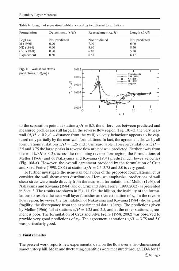
Fig. 11 Wall shear stresspredictions, τw/(ρu2

δ )

-5 0 10 15x/H

-0.003

0

0.003

0.006

0.009

0.012τ w

/(ρu

δ2 )ExperimentsCSF (1998)NK (1984)M (1966)LogLaw

5

to the separation point, at station x/H = 0.5, the differences between predicted andmeasured profiles are still large. In the reverse flow region (Fig. 10c–f), the very near-wall (d/H < 0.2, d = distance from the wall) velocity behaviour appears to be cap-tured only partially by the near-wall formulations. In fact, the agreement shown by allformulations at stations x/H = 1.25 and 5.0 is reasonable. However, at stations x/H =2.5 and 3.75 the large peaks in reverse flow are not well predicted. Farther away fromthe wall (d/H > 0.2), across the remaining reverse flow region, the formulations ofMellor (1966) and of Nakayama and Koyama (1984) predict much lower velocities(Fig. 10d–f). However, the overall agreement provided by the formulation of Cruzand Silva Freire (1998, 2002) at station x/H = 2.5, 3.75 and 5.0 is very good.

To further investigate the near-wall behaviour of the proposed formulations, let usconsider the wall shear-stress distribution. Here, we emphasize, predictions of wallshear stress were made directly from the near-wall formulations of Mellor (1966), ofNakayama and Koyama (1984) and of Cruz and Silva Freire (1998, 2002) as presentedin Sect. 3. The results are shown in Fig. 11. On the hilltop, the inability of the formu-lations to resolve the near-wall layer furnishes an overestimation of τw. In the reverseflow region, however, the formulation of Nakayama and Koyama (1984) shows greatfragility; the discrepancy from the experimental data is large. The predictions givenby Mellor (1966) fail at stations x/H = 1.25 and 2.5, and at the other stations, agree-ment is poor. The formulation of Cruz and Silva Freire (1998, 2002) was observed toprovide very good predictions of τw. The agreement at stations x/H = 3.75 and 5.0was particularly good.

5 Final remarks

The present work reports new experimental data on the flow over a two-dimensionalsmooth steep hill. Mean and fluctuating quantities were measured through LDA for 13


different stations. In particular, the large separated region that was formed on the leeof the hill was characterized through seven different stations. The work characterizedthe mean velocity behaviour for both mean velocity components, showing in detailthe near-wall reverse flow region. The data showed how turbulence production islargely enhanced in the separation region, yielding values of u′2, w′2 and −u′w′ thatare much higher than the values in the upstream undisturbed profile. Complementaryplots illustrating other properties of turbulence, including the local turbulent kineticenergy, the production terms, the local mixing length and the local eddy viscosity willbe presented elsewhere.

In addition, we have performed a numerical simulation of the flow via a finiteelements code, Turbo-2D. The code models turbulence through a κ–ε model and useswall functions to specify the boundary conditions. In the present numerical simulation,we have shown that predictions were very sensitive to the various types of near-wallformulations that were used. All three law-of-the-wall expressions that were spe-cially devised to deal with adverse pressure gradients were capable of predicting thereverse flow region. However, the formulations of Mellor (1966) and of Nakayama andKoyama (1984) much underpredicted the flow velocity. The results of Mellor (1966)and of Nakayama and Koyama (1984) also gave poor predictions for the wall shearstress. Overall, the best mean velocity results in the reverse flow region (X/H =1.25, 2.5, 3.75 and 5.0) were given by the formulation of Cruz and Silva Freire (1998,2002). This fact has been specially corroborated by the very good wall shear-stresspredictions.

Acknowledgements The quality and legibility of this work has been greatly improved thanks to themany helpful comments and suggestions received from one referee. JBRL benefited from a ResearchScholarship from the Brazilian Ministry of Education through CAPES. JBRL is also grateful to theProgramme Alban, European Union Programme of High Level Scholarships for Latin America, iden-tification number E03M23761BR, for the concession of further financial help regarding her stay atOporto University. APSF is grateful to the Brazilian National Research Council (CNPq) for the awardof a Research Fellowship (Grant No 304919/2003-9). The work was financially supported by CNPqthrough Grant No 472215/2003-5 and by the Rio de Janeiro Research Foundation (FAPERJ) throughGrants E-26/171.198/2003 and E-26/152.368/2002. JLAFR and DVS are grateful to the Technologyand Scientific Enterprise Foundation (FINATEC) from the University of Brasilia, for the materialand financial support, which made the computational work possible. FTP is grateful to Prof. MariaFernanda Proença and the Hydraulics Laboratory at Oporto University for all their help in setting upthe flow rig and technical discussions.

References

Arya SPS, Capuano ME, Fagen LC (1987) Some fluid modelling studies of flow and dispersion overtwo-dimensional low hills. Atmos Environ 21:753–764

Athanassiadou M, Castro IP (2001) Neutral flow over a series of rough hills: a laboratory experiment.Boundary-Layer Meteorol 101:1–30

Brison JF, Buffat M, Jeandel D, Serres E (1985) Finite element simulation of turbulent flows usinga two-equation model. In: Numerical methods in laminar and turbulent flow. Pineridge Press,Swansea, UK, pp 563–573

Britter RE, Hunt JCR, Richards KJ (1981) Air flow over a two-dimensional hill: studies of velocityspeedup, roughness effects and turbulence. Quart J Roy Meteorol Soc 107:91–110

Brun G (1988) Development et application d’une méthode d’élement finis pour le calcul desécoulements turbulents fortement chaufées. Thèse de Doctorat, Ècole Centrale de Lyon, 156 pp

Buice C, Eaton J (1995) Experimental investigation of the flow through an asymmetric plane diffuser.Annual research briefs. Center of Turbulence Research, Stanford University, Nasa Ames, pp117–120


Carlson JJ, Johnston JP, Sagi CJ (1967) Effects of wall shape on flow regimes and performance instraight two-dimensional diffusers. J Basic Eng 89 (March):151–160

Coles D (1956) The law of the wake in the turbulent boundary layer. J Fluid Mech 1:191–226Cruz DOA, Silva Freire AP (1998) On single limits and the asymptotic behaviour of separating

turbulent boundary layers. Int J Heat Mass Transfer 41:2097–2111Cruz DOA, Silva Freire AP (2002) Note on a thermal law of the wall for separating and recirculating

flows. Int J Heat Mass Transfer 45:1459–1465Finnigan JJ (1983) A streamlined coordinate system for distorted turbulent shear flows. J Fluid Mech

130:241–258Fontoura Rodrigues JLA (1990) Méthode de minimisation adaptée à la technique des éléments finis

pour la simulation de écoulements turbulents avec conditions aux limites non linéaires de procheparoi. Thèse de Doctorat, Ècole Centrale de Lyon, 152 pp

Gong W, Ibbetson A (1986) A wind-tunnel study of turbulent flows over model hills. Boundary-LayerMeteorol 49:113-148

Grant ALM (1992) The structure of turbulence in the near-neutral atmospheric boundary-layer. JAtmos Sci 49:226–239

Hughes TJR, Brooks A (1979) A multi-dimensional upwind scheme with no crosswind diffusion.Finite element methods for convection dominated flows. ASME-AMD, New York 34:19–35

Kelly DW, Nakazawa S, Zienkiewcz S (1980) A note on upwinding and anisotropic balancingdissipation in finite element approximations to convective diffusion problems. Int J Numer Meth-ods Eng 15(11):1705–1711

Khurshudyan LH, Snyder WH, Nekrasov IV (1981) Flow and dispersion of pollutants over two-dimensional hills. Env Prot Agency Rpt No EPA-600/4-81-067. Research Triangle Park, NC,130 pp

Kim J, Kline SJ, Johnston JP (1980) Investigation of a reattaching turbulent shear layer: flow over aback-ward facing step. J Fluids Eng 102:302–308

Launder BE, Spalding DB (1974) The numerical computation of turbulent flows. Comput Meth ApplMech 3:269–289

Mansour NN, Kim J, Moin P (1989) Near-wall kappa-epsilon turbulence modelling. AIAA J 27(8):1068–1073.

Mellor GL (1966) The effects of pressure gradients on turbulent flow near a smooth wall. J FluidMech 24:255–274

Millikan CB (1939) A critical discussion of turbulent flow in channels and tubes. Proc. 5th Int. Cong.App. Mech. J. Wiley, New YorK, pp 386–392

Nakayama A, Koyama H (1984) A wall law for turbulent boundary layers in adverse pressuregradients. AIAA J 22:1386–1389

Prandtl L (1925) Über die ausgebildete Turbulenz. ZAMM 5:136–139Reneau LR, Johnston JP, Kline SJ (1967) Performance and design of straight two dimensional

diffusers. J Basic Eng 89 (March):141–150Simpson RL, Chew YT, Schivaprasad BG (1981) The structure of a separating boundary layer. Part

1: mean flow and Reynolds stresses. J Fluid Mech 113:23–51Stratford BS (1959) The prediction of separation of the turbulent boundary layer. J Fluid Mech 5:1–16Trupp AC, Azad RS, Kassab SZ (1986) Near-wall velocity distributions within a straight conical

diffuser. Exp Fluids 4:319–331

water tank and numerical model studies of ﬂow over steep...

Documents