1

Water Management in Refining Processes

Amy Frink Timilehin Kehinde

Brian Sellers Department of Chemical, Biological, and Materials

Engineering 5/8/2009

2

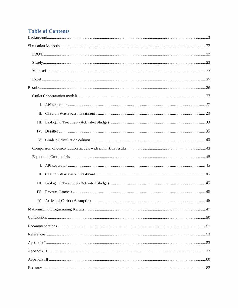
Table of Contents Background .................................................................................................................................................................... 3

Simulation Methods ..................................................................................................................................................... 22

PRO/II ..................................................................................................................................................................... 22

Steady ...................................................................................................................................................................... 23

Mathcad ................................................................................................................................................................... 23

Excel........................................................................................................................................................................ 25

Results ......................................................................................................................................................................... 26

Outlet Concentration models ................................................................................................................................... 27

I. API separator ................................................................................................................................ 27

II. Chevron Wastewater Treatment ...................................................................................................... 29

III. Biological Treatment (Activated Sludge) ......................................................................................... 33

IV. Desalter ........................................................................................................................................ 35

V. Crude oil distillation column ........................................................................................................... 40

Comparison of concentration models with simulation results ................................................................................. 42

Equipment Cost models .......................................................................................................................................... 45

I. API separator ................................................................................................................................ 45

II. Chevron Wastewater Treatment ...................................................................................................... 45

III. Biological Treatment (Activated Sludge) ......................................................................................... 45

IV. Reverse Osmosis ........................................................................................................................... 46

V. Activated Carbon Adsorption .......................................................................................................... 46

Mathematical Programming Results ............................................................................................................................ 47

Conclusions ................................................................................................................................................................. 50

Recommendations ....................................................................................................................................................... 51

References ................................................................................................................................................................... 52

Appendix I ................................................................................................................................................................... 53

Appendix II .................................................................................................................................................................. 72

Appendix III ................................................................................................................................................................ 80

Endnotes ...................................................................................................................................................................... 82

3

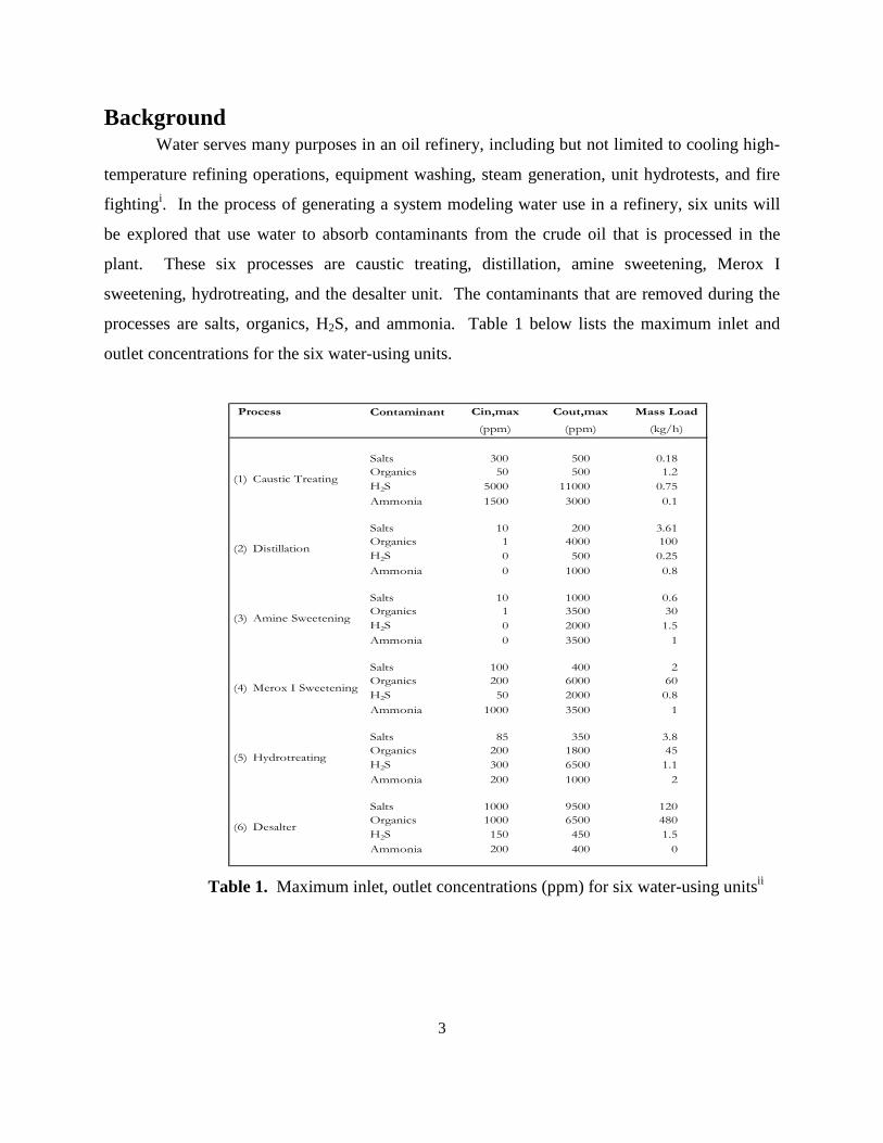
Background Water serves many purposes in an oil refinery, including but not limited to cooling high-

temperature refining operations, equipment washing, steam generation, unit hydrotests, and fire

fightingi. In the process of generating a system modeling water use in a refinery, six units will

be explored that use water to absorb contaminants from the crude oil that is processed in the

plant. These six processes are caustic treating, distillation, amine sweetening, Merox I

sweetening, hydrotreating, and the desalter unit. The contaminants that are removed during the

processes are salts, organics, H2S, and ammonia. Table 1 below lists the maximum inlet and

outlet concentrations for the six water-using units.

Contaminant

Salts 300 500 0.18

Organics 50 500 1.2

H2S 5000 11000 0.75

Ammonia 1500 3000 0.1

Salts 10 200 3.61

Organics 1 4000 100

H2S 0 500 0.25

Ammonia 0 1000 0.8

Salts 10 1000 0.6

Organics 1 3500 30

H2S 0 2000 1.5

Ammonia 0 3500 1

Salts 100 400 2

Organics 200 6000 60

H2S 50 2000 0.8

Ammonia 1000 3500 1

Salts 85 350 3.8

Organics 200 1800 45

H2S 300 6500 1.1

Ammonia 200 1000 2

Salts 1000 9500 120

Organics 1000 6500 480

H2S 150 450 1.5

Ammonia 200 400 0

(6) Desalter

(4) Merox I Sweetening

(5) Hydrotreating

(2) Distillation

(3) Amine Sweetening

(ppm) (ppm) (kg/h)

(1) Caustic Treating

Process Cin,max Cout,max Mass Load

Table 1. Maximum inlet, outlet concentrations (ppm) for six water-using unitsii

4

Figure 1 below gives a schematic of a typical refinery. The water-using units are cirled

in red and the wastewater treatment processes are circled in green.

Figure 1. Refinery schematiciii

Crude desalting is usually the first step in a petroleum refining process. Crude oil enters

into the refining unit from outside storage tanks and contains heavy amounts of contaminants,

including water with dissolved or suspended salt crystals. It is heated by heat exchangers in

order to increase the viscosityiv. A separate water stream is then introduced to the system and

comes into contact with the crude oil, after which the two streams are vigorously mixed over a

mixing valve. Water and crude oil are immiscible solvents and since salt has a higher solubility

in water, the aforementioned salt particles will partition into the water. A schematic of the

desalting process is shown on the following page.

Desalter

Distillation (atmospheric)

Distillation (vacuum)

Hydrotreating Sweetening

Chevron Wastewater Treatment, RO, Biological, API Separator, ACA

5

Figure 2. Single-stage electrostatic desalting systemv

There are two types of distillation: atmospheric and vacuum. After the desalting stage,

the crude oil is heated in heat exchangers and heated to about 750 degrees Fahrenheit before it

enters into an atmospheric distillation unit. Atmospheric distillation separates light end products

like natural gas, naphtha, and gas oil from crude oil. The crude is partially vaporized in a fired

heater before entering the distillation unit flash zone. Superheated steam is introduced through

the column bottom to strip any remaining gas oil from the flash zone liquid. The steam reduces

the hydrocarbon partial pressure thereby reducing vaporization temperature. An atmospheric

column is shown below:

Figure 3. Atmospheric distillation unitvi

6

Following atmospheric distillation, the heavy bottoms product containing heavier

fractions of crude oil is sent to a vacuum distillation tower where distillation under very low

pressures (usually 25 to 40 mmHgvii) is carried out. Temperatures required for atmospheric

distillation of heavier components would be too high and would result in cracking of

hydrocarbons. By lowering the distillation pressure and introducing steam to the system (to

improve vaporization), heavier products can be distilled. Prior to entering the distillation

column, the topped crude is heated in a furnace to temperatures of about 750-850 degrees

Fahrenheit. After distillation, different fractions of heavy components exiting the system pass

through pumps and heat exchangers. A vacuum distillation column is shown below:

Figure 4. Vacuum distillation unitviii

Caustic treating is a refining process that uses an aqueous solution of NaOH to absorb

acid gas compounds, like H2S, CO2, and mercaptans, found in natural gas or liquid hydrocarbon

streams. Crude oil fractions that exit from the vapor stream in a distillation tower contain sulfur-

based compounds, which are odiferous and corrosive. Following distillation, this light crude

stream goes through amine treatment, which removes many of the mercaptans and helps to

reduce the load that is sent to caustic treatmentix. A caustic solution of normally 15 wt% NaOH

and higher is then introduced into an absorption tower where it comes into contact with the

7

passing stream of light crudes and extracts the contaminantsx. Caustic treating is normally used

to clean liquefied natural gas (LNG) and diesel fuels. A diagram of a caustic treatment unit is

shown below.

Figure 5. Caustic treating processxi

Amine sweetening is a process whereby aqueous solutions of alkanolamines (such as

monoethanolamine or diethanolamine) absorb contaminants like hydrogen sulfide (H2S), carbon

dioxide (CO2), and mercaptans from a passing stream of natural gas. The absorption process is

called sweetening because it eliminates the bitter odor coming from the sour feed making the

clean gas smell “sweet”. The acid gas contents are removed through chemical reactions with the

amines in the amine solution and come out of the absorber in the rich amine liquid solution. A

flash tank is usually installed at the absorber outlet to reduce flash any hydrocarbons that may be

in the feed, thereby removing them from the acid gas productxii. A process flow diagram of an

amine-sweetening unit is shown in Figure 6.

8

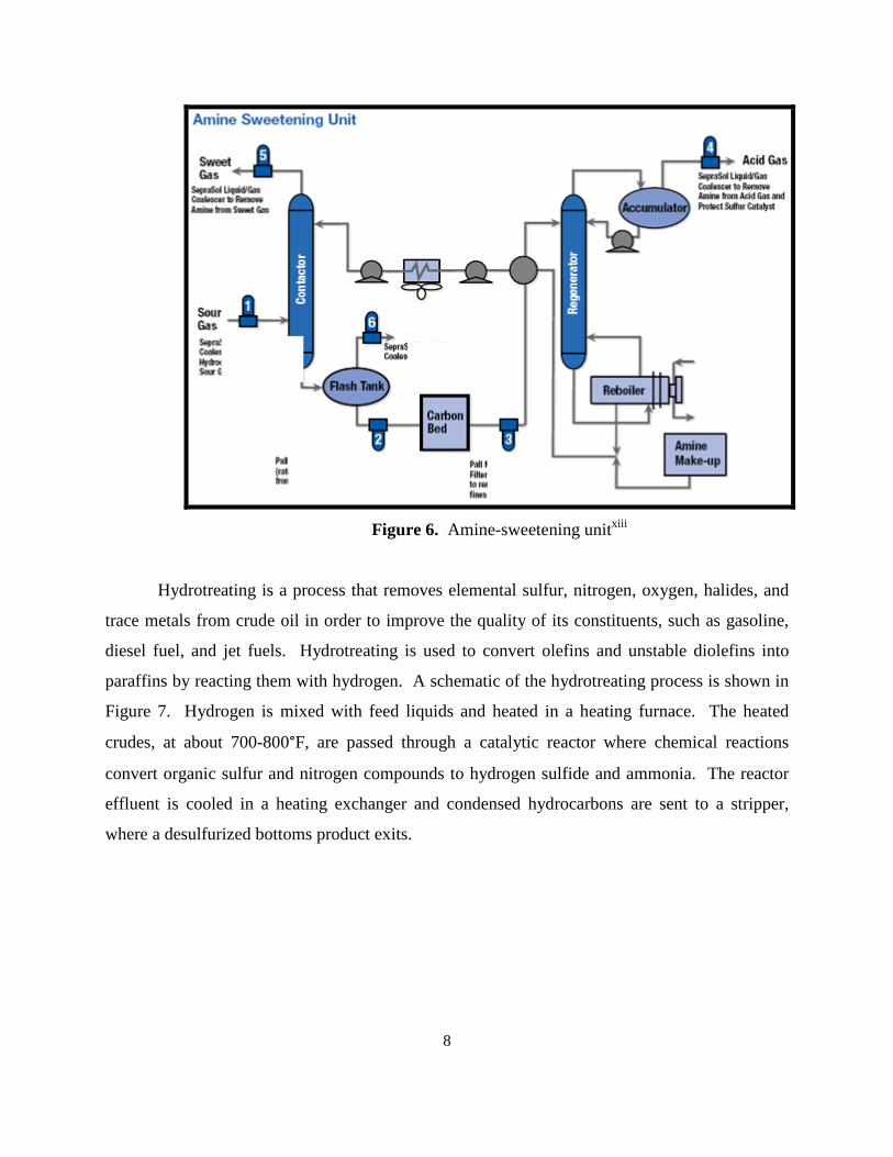
Figure 6. Amine-sweetening unitxiii

Hydrotreating is a process that removes elemental sulfur, nitrogen, oxygen, halides, and

trace metals from crude oil in order to improve the quality of its constituents, such as gasoline,

diesel fuel, and jet fuels. Hydrotreating is used to convert olefins and unstable diolefins into

paraffins by reacting them with hydrogen. A schematic of the hydrotreating process is shown in

Figure 7. Hydrogen is mixed with feed liquids and heated in a heating furnace. The heated

crudes, at about 700-800°F, are passed through a catalytic reactor where chemical reactions

convert organic sulfur and nitrogen compounds to hydrogen sulfide and ammonia. The reactor

effluent is cooled in a heating exchanger and condensed hydrocarbons are sent to a stripper,

where a desulfurized bottoms product exits.

9

Figure 7. Hydrotreatment unitxiv

API separators separate suspended solids and oil from wastewater streams based on

differences in specific gravities between the oil and the wastewater. The differential density is

much smaller for oil and wastewater than for suspended solids and wastewater. Thus, the oil

globules will rise through the water, suspended solids will sink to the bottom, and the wastewater

containing some small amounts of oil particles will exit as the middle layer. After separation, the

oil in the top layer is skimmed off and re-processed and the sedimentation from the bottom of the

separator is removed using a sludge pump.

The particles settling in an API separator operate on the basis of Stokes Law: the

contaminant particles fall through the viscous fluid by their own weight due to a gravitational

force. The upward drag of the small particles (which are assumed to be spheres) combine with

the buoyancy force balances the gravitational force thereby creating a settling velocity, which is

the velocity at which the particles settle. The settling velocity, also termed the terminal velocity,

is given by:

( ) 2

9

2gRV OWt ρρ

µ−= Equation 1

10

where Vt is the settling velocity in cm/s, µ is the fluid viscosity in poise, ρW is the density of

water at the design temperature in g/cm3, ρO is the density of oil at the design temperature in

g/cm3, g is the gravitational constant (981 cm/s2), and R is the radius of the particle which will be

removed in cm. Typically, a particle with a radius no smaller than 0.015 cm, will settle out of

the water. A schematic of an API separator is shown below.

Figure 8. API Separatorxv

Reverse osmosis

Theory of reverse osmosis

Reverse osmosis is a process by which dissolved solutes are separated from a solution by

a pressure-driven membrane that applies the preferential diffusion for separation. The solution to

be separated on one side of the membrane known as the feed is separated by a membrane filled

with pure water on the other side. Due to difference in the concentrate between the feed and

permeate side instability is created, water then flows from the pure side to the feed to equilibrate

the system. The water level in the solution will rise to a point, which is equal to the osmotic

pressure, π, of the concentrated solution. When this occurs, the water flux across the membrane

to the permeate is equal to that to the feed and equilibrium is reached. At this point of

equilibrium, the driving force generated to move the water molecules is then terminated. This

process is known as the osmosis process.

11

Figure 9. Osmosis and reverse osmosis processes

In reverse osmosis, high pressure is applied at the feed and a differential pressure is

created between the permeate and feed sides of the membrane. This results into a pressure

change, the system then becomes unstable allowing the flow of water from the feed stream

through the membrane to the pure water side (permeate). As water passes through the

membrane, the solutes are rejected at the membrane surface increasing the concentration of the

feed stream which flows out of the process as a stream called the concentrate. The permeate

exits the process at atmospheric pressure, while the concentrate stream leaves the membrane

element at high pressure is approximately equal to the feed pressure.

The rate of flow of water molecules in a unit area of the membrane (also known as the

water flux) through the membrane is the product of the driving force and the transfer rate as

defined by the below equation:

JW = kw · (∆P – ∆π) Equation 2

where: JW = volumetric flux of water (L/m2·s)

kW = mass transfer coefficient of water flux (L/m2·s·atm)

∆P = (PF – PP) = hydraulic pressure change (atm)

∆π = (πF – πP) = change in osmotic pressure in the feed and

permeate (atm)

The flow of the solutes (salt) through the membrane is given by the equation below:

JS = kS · (∆C) Equation 3

where: JS = mass flux of solute (kg/m2·s)

kS = mass transfer coefficient of solute (L·S/m2)

12

The osmotic pressure of the feed is calculated using van’t Hoff law for dilute solutions as in the

expression below:

π = cRT Equation 4

where : c = concentration of solute in feed/permeate (mol/L)

R = gas constant ~0.0820578 (L·atm)/(g-mol·K)

T = temperature of solution (K)

Membrane material

The force directed towards the membrane for the separation of solutes from water based

on the physical and chemical properties of the solutes to be removed and the material of the

membrane. The resistance to flow through the membrane is inversely related to the thickness

which means that for high efficiency, the membrane has to be extremely thin. For a reverse

osmosis, the thickness of the membranes ranges from about 0.1 to 2 µm. This extreme size of

the material makes the membrane lack structural reliability as a result, membranes usually

comprise of several layers with low porosity. The ideal material is one that can produce a high

flux without clogging or fouling and is physically durable and chemically inactive. The

materials most widely used in reverse osmosis are the cellulosic derivatives and polyamide

derivatives (Crittenden).

Process application in wastewater treatment

In wastewater treatment process, reverse osmosis is a technology used for the removal of

various inorganic contaminants. However, the main problem with the reverse osmosis

technologies in the waste water treatment industry is the disposal of the concentrates and fouling

that occurs on the membrane over a period of time as pressure is increased. However, to prevent

this from occurring, the wastewater is pretreated by scaling which adjust the PH value, changing

the solubility of the precipitates of inorganic contaminants that could be formed during operation

(Hendricks).

13

Mathematical model

QP, CP, PP

QF, CF, PF

QC, CC, PC

A mass balance around the membrane pressure vessel process results to the following equations:

Membrane mass balance

QF = QC + QP Equation 5

CFQF = CC·QC + CP·QP Equation 6

where:

CC = concentrate of solute in concentrate water (kg/m3)

CP = solute concentrate in permeate water (kg/m3)

CF = solute concentrate in feed water (kg/m3)

QP = permeate flow (m3/s)

QF = feed flow (m3/s)

QC = concentrate flow (m3/s)

The flow rate of water molecules in the permeate is related to the water flux by the equation

shown below:

QP = JW x Area of membrane Equation 7

The flux of the solutes is also related to the flux of water by the equation below:

JS = CP · JW Equation 8

The combination of the solute flux in equations 2 and 8, and rearranging the equation, the

concentration of salts in the treated water (permeate) CP, was determined. The final equation that

relates the concentration out at the permeate was found to be:

14

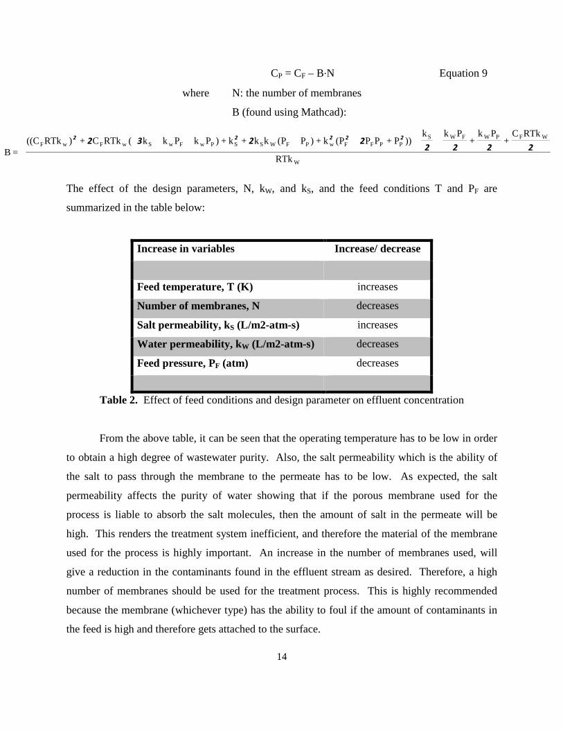
CP = CF – B·N Equation 9

where N: the number of membranes

B (found using Mathcad):

The effect of the design parameters, N, kW, and kS, and the feed conditions T and PF are

summarized in the table below:

Increase in variables Increase/ decrease

Feed temperature, T (K) increases

Number of membranes, N decreases

Salt permeability, kS (L/m2-atm-s) increases

Water permeability, kW (L/m2-atm-s) decreases

Feed pressure, PF (atm) decreases

Table 2. Effect of feed conditions and design parameter on effluent concentration

From the above table, it can be seen that the operating temperature has to be low in order

to obtain a high degree of wastewater purity. Also, the salt permeability which is the ability of

the salt to pass through the membrane to the permeate has to be low. As expected, the salt

permeability affects the purity of water showing that if the porous membrane used for the

process is liable to absorb the salt molecules, then the amount of salt in the permeate will be

high. This renders the treatment system inefficient, and therefore the material of the membrane

used for the process is highly important. An increase in the number of membranes used, will

give a reduction in the contaminants found in the effluent stream as desired. Therefore, a high

number of membranes should be used for the treatment process. This is highly recommended

because the membrane (whichever type) has the ability to foul if the amount of contaminants in

the feed is high and therefore gets attached to the surface.

RTk

RTkC+

Pk+

Pkk))P+PPP(k+)PP(kk+k+)PkPkk(RTkC+)RTkC((

=BW

WFPWFWSPPFFwPFWSSPwFwSwFwF

22222232

22222

15

The table below summarizes the optimum conditions and design parameters to achieve high

degree of purity in the wastewater.

Parameters and effects

Feed temperature, T (K) Decrease temperature, negligible effect at extreme low temperature

Number of membranes, N Increase the number used, high degree of purity can be attained

Salt permeability, Ks (L/m2-atm-s) Choose material with low salt permeability, possibly zero

Water permeability, Kw(L/m2-atm-s) Choose material with high water permeability

Feed pressure, PF (atm) Increase the pressure at the feed to allow high degree of diffusion at membrane

Table 3. Feed conditions and design parameters to be considered for process design

Activated Carbon Adsorption

Theory of adsorption

Adsorption is a process by which molecules of substances present in a liquid phase are

attached on the surface of a solid matter and removed from the liquid phase. The process

involves the molecules in the gas or liquid phase diffuse to the surface of the solid and stay there

by chemical bonding or weak intermolecular forces. The solid phase particle which provides the

bonding sites is known as the adsorbent and the substance in the adsorbed state is called the

adsorbate.

There are two main types of adsorption which are the physisorption and the

chemisorption. The physisorption is when the adhesive forces are of physical nature and

adsorption is relatively weak and the amount of heat evolved for a mole of gas adsorbed is

usually less than 20 kJ (Laidler). For the chemisorption, the adsorbed molecules are bonded to

the surface by covalent forces which are stronger than intermolecular forces between the

molecules of the adsorbate. In chemisorption which is usually applied in industries, after the

surface has been covered with a monolayer of adsorbed molecules, it is said to be saturated and

16

additional adsorption occurs on the layer that already exists. However, Langmuir emphasized

that adsorption formation is of unimolecular layer and once formed adsorption ceases but

multilayer can exist for physisorption.

Adsorbent

Adsorbents used in industries are generally synthetic microporous solids: activated

carbon, molecular sieve carbon, activated alumina, silica gel, zeolites and bleaching clay. The

most important characteristics of adsorbents are pore volume, the pore distribution and the

geometry of the particles of the adsorbent. The table below shows the properties of the

commonly used activated carbon.

Filtrasorb 100 Filtrasorb 200 Filtrasorb 300 Filtrasorb 400

Surface area, BET (m2/g) 800-900 800-900 950-1050 1000-1200

Apparent density (g/mL) no data ≥0.48 ≥0.48 ≥0.44

Wetted density (g/mL) 1.4-1.5 1.4-1.5 1.3-1.4 1.3-1.4

Effective size (mm) 0.8-1.0 0.55-0.75 0.8-1.0 0.55-0.75

Uniformity coefficient 2.1 1.9 2.1 1.9

Abrasion number 75 75 78 75

PropertyActivated Carbon

Properties of Activated Carbon

Table 4. Properties of Activated Carbon

Process description

At equilibrium, the rate of adsorption on the surface of the adsorbent is equal to the rate

at which desorption occurs. When this occurs, an increase in the residence time of the adsorbate

in the column of adsorbate has no effect. The adsorption process can be described as in the usual

chemical reaction as shown below:

C + X ↔ C·X Equation 10

where:

C = adsorbent concentration (kg/m3)

C·X = concentration of the sites occupied by adsorbate molecules (kg adsorbate adsorbed/kg

adsorbent/m3 solution)

X = adsorbate sites not occupied per unit adsorbent in a unit volume (kg unoccupied

adsorbate/kg adsorbent/m3 solution)

17

At equilibrium, the rate of adsorption and desorption are equal. The equilibrium constant can be

then introduced as below.

[ ]

[ ] [ ]** XC

XCKKeq

⋅== Equation 11

where: Keq = K = adsorption equilibrium constant

[C]* = adsorbate concentrate, C, at equilibrium

(kg adsorbent/m3 solution)

Langmuir Isotherm

Adsorption isotherm relates the amount of substance attached to the surface of the

adsorbent to the amount in the solution at a defined temperature. The Langmuir isotherm which

is used for the process assumes that the surface of the activated carbon is homogeneous and as

mentioned previously adsorption occurs in a single layer.

KC

KCXX max= Equation 12

where: K = Langmuir equilibrium constant = Keq

Xmax = maximum amount of adsorbate in solid phase per adsorbent (kg

adsorbate/kg adsorbent)

C = concentration in solution at equilibrium (kg adsorbate/m3 solution)

It is assumed that the internal (pore) diffusion is rate controlling in the adsorption

process. It is also assumed that the geometry of the activated carbon particle is spherical and all

the assumptions made for the Langmuir isotherm is also used. Finally, the bed is assumed to be

a batch process in a tank of volume, V.

Mathematical model

To design the activated carbon adsorption process, the fixed bed was chosen rather than

the slurry adsorption. This is due to the fact that the fixed bed is more efficient and the bed can

be regenerated not disposed as in the case of slurry adsorption.

Assuming the process is a plug flow of the wastewater through the bed is at a constant

interstitial velocity, there is no axial dispersion and the temperature is constant throughout the

18

process (isothermal); the mass balance on the solute flowing through a bed length z at

differential length ∆z is given by the equation:

( )

01 =

∂∂⋅−+

∂∂+

∂∂

t

q

z

Cu

t

C

εε

Equation 13

However, when the axial dispersion and transfer of mass from the solute to the activated carbon

is not neglected as initially assumed, the equation above is modified to a partial differential

which is given below:

01

2

2

=∂

∂⋅

−+∂

∂+

∂∂+

∂∂

+∂

∂−

t

q

t

C

z

VC

z

CV

z

CD p

pb

bbb

L εερ Equation 14

In the above equation, the DL is known as the term which accounts for the axial dispersion with

diffusion to the activated carbon bed, the second term is related to the change in velocity of flow

axially. This equation has to be solved numerically, but an analytical solution can be found

when the equation is made simple. Klinkenberg approximation was used to determine the

solution with certain assumptions which include that the axial dispersion can be ignored, the

fluid velocity is constant and the mass transfer model is linear. The Klinkenberg approximation

is as below:

++−+≈ετ

ετ8

1

8

11

2

1erf

C

C

F

Equation 15

where:

−=s

s

u

kKz 1ε Dimensionless distance coordinates

−=u

ztkτ Dimensionless time coordinate corrected for displacement

Using this formula, the effluent concentration was estimated to be approximately zero based on

the residence time in the column.

19

Chevron waste water treatment

Chevron waste water treatment (WWT) strips hydrogen sulfide and ammonia from sour

water generated in petroleum refineriesxvi. The two-stage stripping process produces separate

purified ammonia and hydrogen sulfide streams, wherein the hydrogen sulfide can be sent to

sulfur recovery units, the ammonia can be sold commercially or used again in Selective Catalytic

or Selective Non-catalytic Reduction units in the refinery, and the purified wastewater can either

be sent to end-of-pipe treatments or reused. A process-flow diagram for a Chevron water

treatment plant is shown below.

Figure 10. Chevron Wastewater Treatment Plantxvii

Biological treatment

Biological treatment operates on the idea that microorganisms present in wastewater will

feed on the carbonaceous organic matter in the wastewater and repopulate in an aquatic aerobic

environment. With a sufficient oxygen supply and an organic material food supply, the bugs

(bacteria) will consume and metabolize the organic waste and transform it into cell mass, which

settles in the bottom of a settling tank.

20

Most biological treatment plants have two forms of operation: primary and secondary.

Primary treatment involves the physical removal of solids and secondary treatment involves the

biological removal of dissolved solidsxviii . Secondary treatment mainly uses biological treatment

processes, whereby the introduction of microorganisms to the system creates solids which

precipitate out and are collected in the settling tank. Three common options for secondary

treatment include:

I. Activated sludge

II. Trickling filters

III. Lagoons

The treatment that will be modeled in this project is the activated sludge system. The

wastewater influent is sent through an aeration tank where air is pumped through the bottom of

the tank and rises through the water in the form of bubbles. The purpose for this is two-fold: air

provides oxygen to the water and creates turbulent conditions ideal for organic material

consumptionxix. The wastewater is then sent through what is called a secondary clarifier. The

clarifier is a settling tank that separates the used cellular material from the treated wastewater.

The cellular material sinks to the bottom of the basin whereby it is either sent back to aeration

tank to assist in producing new bacteria or sent as sludge for anaerobic treatment. A schematic

of the process is shown on the next page in Figure 11.

21

Figure 11. Activated sludge systemxx

where:

Q = flowrate of influent [m3/d]

QW = waste sludge [m3/d]

Qr = flowrate in return line from clarifier [m3/d]

V = volume of aeration tank [m3]

S0 = influent soluble substrate concentration (bsCOD) [m3/d]

S = effluent soluble substrate concentration (bsCOD) [BOD g/m3] or [bsCOD g/m3]

X0 = concentration of biomass in influent [g VSS/m3]

XR = concentration of biomass in return line from clarifier [g VSS/m3]

Xr = concentration of biomass in sludge drain [g VSS/m3]

Xe = concentration of biomass in effluent [g VSS/m3]

22

Simulation Methods

Several different methods were used in this study to simulate real-life water-using and

water treating process units. PRO/II, Steady, Mathcad, and Excel were used to generate points

by varying inlet system parameters, like temperature, pressure, flowrate, etc. These points were

then analyzed to find the nature of correlations between components varied and outlet

concentration. The Casestudy function in PRO/II has the capability of varying more than one

inlet parameter at once (maximum used in this study was six) and this eased the workload. The

Excel files made by the researchers were used mostly for cost analyses purposes.

PRO/II The primary simulation program used in this study was PRO/II. Its proven accuracy in

predicting results from specifications of inlet parameters and its applicability to the processes

currently being modeled were the reasons for its use. The H2S stripper, NH3 stripper, amine

sweetening, and atmospheric columns were modeled in PRO/II as distillation columns. The H2S

differed slightly from the other distillation columns in that it contained only a partial reboiler and

not a partial condenser. A snapshot of the crude oil distillation unit is shown in Figure 12.

Figure 12. Snapshot of Pro/II crude oil distillation unit

23

Steady The simulation program used to model the activated sludge system was a computer

program called Steadyxxi. Steady is a steady-state wastewater treatment plant modeling program

developed by researchers at the University of Texas that characterizes wastewater in terms of

water quality assessment procedures, like BOD5, TSS, VSS, TKN, and NH3-N. The model

assumes steady-state conditions for influent contaminants to a plant and calculates a plant-wide

mass balance and general dimensions of the unit processes involved. Steady has the capability of

modeling a full activated sludge system, complete with a source stream, aeration tank, clarifier

tank with recycle, sludge stream, and a wastewater effluent stream. A snapshot of the file made

in this study is shown below.

Figure 13. Snapshot of Steady file with activated sludge model and mass balance summary

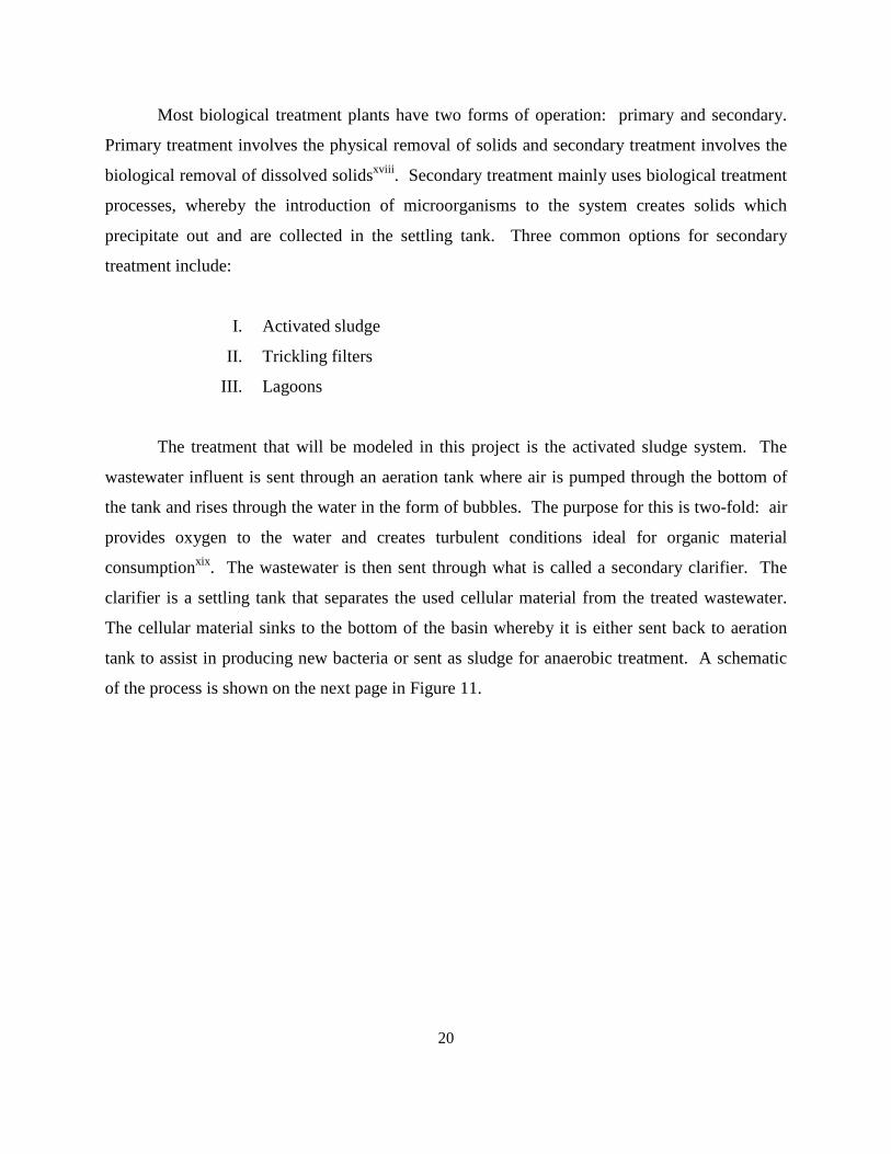
Mathcad Mathcad was used to generate points for the API separator and the reverse osmosis

system. System parameters and inlet stream variables were varied and points were generated to

be input to GAMS as tables. A screenshot of the Mathcad file simulating the API separator is

shown in Figure 14.

24

Figure 14. Snapshot of Mathcad file for API separator

25

Excel Excel files were made for the API separator and the Chevron Wastewater Treatment plant

to model the processes and the cost of the treatment unit. A snapshot is shown in Figure 15.

Figure 15. Snapshot of API separator Excel file

Simulations were run in PRO/II, Steady, Mathcad, and Excel, varying any and all

parameters that could be varied. Inlet parameters in PRO/II were varied based on the model

being used and they include, but are not limited to, column efficiency, number of trays, inlet

temperature, inlet concentration, pressure, reboil and/or reflux ratio, and feed flowrate. A case

study was performed for each simulation in PRO/II and results were exported to Microsoft

Excel. Graphs plotting outlet concentration (dependent variable) vs. each inlet parameter

(independent variable) were then generated to find the relationship between the two variables.

Whatever shape the points in the graph appeared to take was the basis of determination of which

type of regression (linear or non-linear) would be performed. So, for instance, if the graph

appeared to follow a straight line, a linear regression was performed. If the graph had some

26

curvature to it, a non-linear regression (including exponential fit, power law, or logarithmic) was

performed. The regression which produced the highest coefficient of determination, R2, was

kept and regarded as the best fitting line. The graph with the highest coefficient of determination

was kept because it represented the smallest different between the actual and predicted values for

that curve. All R2 and regressions were performed in and by Excel algorithms.

After graphs were generated in Excel, a model was guessed that represented an outlet

contaminant concentration as a function of all of the aforementioned inlet variables. This model

was essentially based on adding together all of the best fit equations of the component curves

that were found to have an effect on effluent concentration. For instance, if Cout were found to

depend on pressure in the form Cout = a*ln(P)b as determined by non-linear regression in Excel

and temperature in the form Cout = c*T + d as determined by linear regression in Excel, then the

resulting model would be Cout = a*ln(P)b + (c*T + d). Parameters a-d were guessed to have the

same values as each component curve did in Excel. All data points and the guessed model were

entered into Polymath and Polymath was left to perform a final non-linear regression.

It’s worth mentioning that although it’s probable that these parameter effects are not

additive and probably have some co-dependence on each other, it will not matter in obtaining an

end result. There is not one right answer in the final model. For any equation guessed as a

model, Polymath takes the non-linearities into account if one uses non-linear data point

regression. As long as the numbers converge and the simulation program used to generate the

data points is accurate, the predicted model will be accurate as well. All results obtained in this

study converged under the maximum number of iterations.

Results Two types of models were generated in this study: outlet concentration models and

equipment cost models. The outlet concentration models describe the outlet contaminant

concentration being investigated in units of parts per million (ppm) as a function of inlet

parameters such as feedrate (ton/hr), pressure (psia), temperature (°F), number of trays (N), tray

efficiency (η), etc. These types of models were made for the API separator, H2S stripper, NH3

stripper, biological treatment (activated sludge), activated carbon adsorption treatment, reverse

27

osmosis, and the atmospheric distillation column. The equipment cost models were made for the

API separator, Chevron Wastewater Treatment plant, activated sludge, and the reverse osmosis

units. They describe process machinery cost in terms of dimensional parameters (length, width,

height), number of trays, reboil ratio, etc. Results are shown in the proceeding sections.

Outlet Concentration models

I. API separator

The API separator was modeled under the assumption that all of the particles coming into

the separator follow a normal distribution, also called a Gaussian distribution. All particles

ranged in size from miniscule to some maximum measured size and the majority of particles lay

somewhere near the average mean particle size. Outliers exist (i.e. particles very large or very

small), but they are present in small quantities and of course, no particles are seen beneath the z

= 0 line on the Gaussian curve. Particles cannot have a negative radius. As the contaminant

particle enters the separator, it has a horizontal velocity vx as well as a vertical settling velocity

vy. The time for a particle to reach the other end of the API Separator (Lt ), that is to travel its

length L is determined by:

Lx

Lt

v= Equation 16

But vx is given by the flowrate F divided by the cross sectional area A given by the product of

width and height, that is A= W*H. Therefore

( ) { }/L

L L H W Vt s

F H W F F

⋅ ⋅= = =⋅

Equation 17

where V is the volume of the API separator. At the same time, the time that a particle that is at

height h at the beginning of the separator will reach the top is:

( ) ( )h

y

H ht s

v

−= Equation 18

The settling velocity of a particle with radius r is given by Stokes Law seen previously in

Equation 1:

( ) 22

9y W Ov grρ ρµ

= − Equation 19

28

Thus:

( ) 2

9 ( )

2hW O

H ht

gr

µρ ρ

−=−

Equation 20

If we now equate h Lt t= , we will obtain the radius of the particle that will exactly reach the top, if

started at height h.

( ) 2

9 ( )

2h LW O

H h Vt t

gr F

µρ ρ

−= = =−

Equation 21

The radius is then given by:

( )9 ( )

ˆ2 W O

H h Fr

gV

µρ ρ

−=−

Equation 22

This equation for ̂r was assigned as the critical radius, above which, all particles separate and

will be removed from the wastewater (and stay in the API separator). Below which, particles are

carried with the wastewater effluent stream (particles smaller that ̂r will stay in the exiting water).

Finally, assuming a Gaussian distribution of particle sizes, we find that the fraction of particles

hy that started at height h that are retained is:

( )

( )

2

2

3

ˆ

3

0

43

43

sr

sr

r r

rh r r

r e dr

y

r e dr

σ

σ

π

π

− −∞

− −∞

=

∫

∫

Equation 23

Being a normal density function, finding the mass of contaminant at any given time involves a

simple multiplication of the density (g/cm3) and the volume (cm3). Now, the particles are

uniformly distributed in height. Then, the total fraction of contaminants removed is:

0

1H

hz y dhH

= ⋅∫ Equation 24

Therefore,

( )

( )( )

2

2

39 ( )

2

03

0

431

43

sr

W O

sr

r r

H h FH gV

r r

r e dr

z dhH

r e dr

σµρ ρ

σ

π

π

− −∞

−−

− −∞

=

∫∫

∫

Equation 25

29

The outlet concentration of organics is then given by:

(1 )Org Orgout inc z c= − Equation 26

We conclude that ( , , )Org Org Orgout out inc c c V H= . In doing this we are assuming that the distribution of

particles is known (it is Gaussian with known mean and std. dev). In addition, an underlying

assumption exists that temperature does not significantly affect the densities of water and the

organic phase. A pictorial representation of the normal density function is seen below.

The area that is shaded is the percentage of the contaminants (oil or suspended solids) removed

from the influent wastewater. All particle sizes are represented in the normal distribution, thus

the area under the Gaussian curve is 1, where 1 represents the entire range of contaminants sizes

from 0 to rmax. The table generated from simulating the numerical integration in Mathcad is seen

in Appendix I.

II. Chevron Wastewater Treatment

As stated before, the Chevron Wastewater Treatment consists of a hydrogen sulfide

stripper followed by an ammonia stripper. The H2S, with a partial reboiler, strips H2S from the

influent wastewater leaving mostly H2S and a negligible amount of ammonia in the vapor

stream. The wastewater then enters into an ammonia stripper, containing a partial reboiler and a

partial condenser, where ammonia is stripped from the wastewater. The curve for the hydrogen

sulfide stripper is shown below.

z

( )9 ( )

ˆ2 W O

H h Fr

gV

µρ ρ

−=−

f(z)

Removed from wastewater

Stays

30

From points 1-11, the mole fraction of hydrogen sulfide coming into the stripper was varied.

From points 12-21, the number of trays was varied. From points 22-55, tray efficiency was

varied from 0.56 through 0.89. From points 56-177, the case study function was used in Pro/II

where the feedrate was varied by increments of 1 kg/hr and the result was the outlet

concentration of H2S. From points 178 on, the inlet temperature was varied. It’s important to

mention that reboiler duty and inlet pressure were run as parameters in the case study in Pro/II,

but the outlet concentration of H2S was found to not be affected by it. A model was guessed and

the result of non-linear regression in Polymath is as follows:

( ) ( )( ) 0158.0700,21

0012.010011.1014.00024.0077.7

,2

,4138.0039.0079.0

, 22

3,

2

++

⋅−⋅+−−=−

−−−

aysNumberoftr

CCxeeppmC SHinSHinTC

SHoutNHin η

Equation 27

The Polymath report for H2S is seen in Appendix I.

From Figure 10 on page 19, it is clear that the liquid stream that exits from the bottom of the

hydrogen sulfide stripper is the entering stream ammonia str9pper. Thus, the outlet

concentration of the H2S stripper is the inlet concentration of the NH3 stripper. The component

31

H2S was the contaminant that was modeled in this study. The non-linear regression graph is

shown below.

In this case, case study function was used rather than single-handedly generating points, which is

tedious. A step size of 100 variations was specified and run in PRO/II. Inlet parameters were

specified to be overall column tray efficiency, feedrate (ton/hr), inlet pressure (psia), reflux ratio

(by changes of 0.5), and inlet temperature (degrees Fahrenheit) was varied. The result was outlet

concentration of H2S and given in units of ppmw.

( )238.0105.7752.0527.04436000

0613.000008069.01546057.00065.000068.047.0

,2941.2

025.0697.0,

2,

2

33

++−−−

+++−−=−

−

SHin

TNNHinNHout

CP

RFReeCFFppmC

ηη

Equation 28

32

An inequality exists that must be able to find optimal column diameter based on flowrate. From

Seader and Henley’s Separation Process Principlesxxii:

( )

−=

Vdf

VT AAfU

VMD

ρπ /1

4 Equation 29

where: V = molar vapor flow rate

MV = molecular weight of the vapor

f = the fraction of flooding, typically taken as 0.80

Uf = flooding velocity = 2

12

1

3

4

−⋅

V

VL

D

p

C

gd

ρρρ

ρV = density of the vapor, ρL = density of the liquid

dp = particle diameter, g = gravity, CD = drag coefficient

( )

≥

≤≤−

+

≤

=

0.1,2.0

0.11.09

1.01.0

1.0,1.0

LV

LVLV

LV

d

F

FF

F

A

A

5.0

=

L

V

V

LLV VM

LMF

ρρ

Equation 30

So, the procedure for determining this inequality is to first calculate FLV (abscissa ratio) and then

choose one of three options:

Case Inequality that must be satisfied Result

1 1.0

5.0

≤

=

L

V

V

LLV VM

LMF

ρρ

( )[ ] ( )[ ]

⋅⋅⋅−⋅⋅=

VVVLDp

VT

Cgd

VMD

ρπρρρ 90.0/3/480.0

4

21

21

2 0.11.0

5.0

≤

=≤

L

V

V

LLV VM

LMF

ρρ

( )[ ] ( )[ ]

⋅

−⋅⋅−⋅⋅

=

VL

V

V

LVVLDp

VT

VM

LMCgd

VMD

ρρρπρρρ 9/8/3/480.0

45.0

21

21

3 0.1

5.0

≥

=

L

V

V

LLV VM

LMF

ρρ

( )[ ] ( )[ ]

⋅⋅⋅−⋅⋅=

VVVLDp

VT

Cgd

VMD

ρπρρρ 80.0/3/480.0

4

21

21

Table 5. Total column diameter as a function of liquid and vapor flowrates

33

III. Biological Treatment (Activated Sludge)

The most commonly used biological treatment is the activated sludge processxxiii , where

microorganisms present in wastewater feed on the organic constituents thereby purifying the

water. Since activated sludge is the most common process, it was the one modeled. As

mentioned before, the program Steady developed by professors at the University of Texas was

used to simulate an activated sludge process. The activated sludge simulation required outlet

concentrations of TBOD5 (mg/L) and SBOD (mg/L) to be specified, and since no nitrification

was occurring in the process, the only outlet concentration that varied was the outlet

concentration of the TKN (mg/L). This was the contaminant that was modeled. Results from the

non-linear regression are shown below.

From points 1-8, inlet concentration of TBOD5 (mg/L) was varied. From points 9-16, inlet

concentration of TKN (mg/L) was varied. From points 17-23, inlet concentration of NH3—N

(mg/L) was varied. From points 24-31, the Y value, which is the biomass yield, was varied.

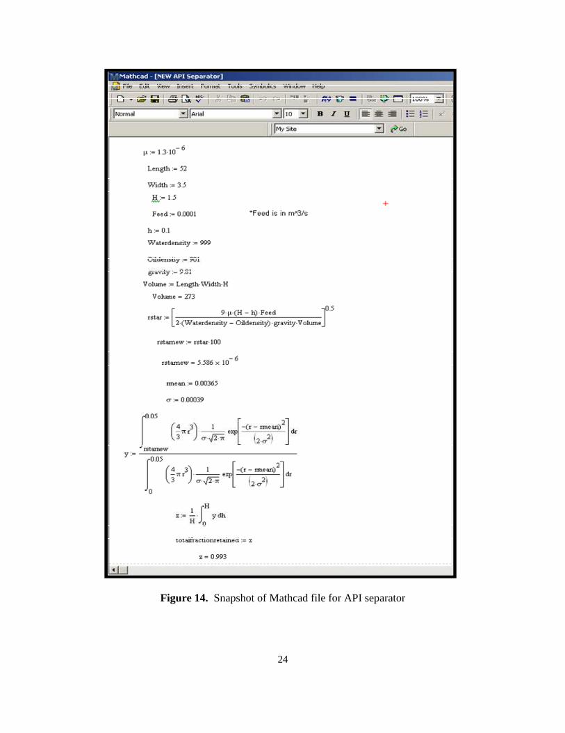
34

Biomass yield is the grams of biomass produced per gram of substrate utilized [g VSS/g COD

used]. From points 32-38, kd was varied and kd is the endogenous decay coefficient [g VSS/g

VSS·d]. From points 39-45, the mean cell residence time (MCRT), the amount of time a

contaminant stays in the process, was varied. From points 46-52, the ratio of mixed liquor

volatile suspended solids to mixed liquor suspended solids was varied. The final result is given

below:

( ) 243625.1208.04.13228784.016.013527.0

0026.0,,

01.0, 35,

+−++−++−=

−

−MLSS

MLVSS

dNNHinTKNineffluentTKN eMCRTkYCCCppmwCTBODin

Equation 31

The sludge that exits from the secondary clarifier is rich in the microorganisms used to eat the

contaminants. This stream was also modeled to aid the pre-treatment process for this stream.

Regression graph results are shown below:

35

Parameters were varied in the same manner as for the effluent wastewater stream, however, an

extra parameter was found to make a difference in outlet TKN concentration; [mgBOD/mg

VSS]. The outlet TKN concentration in the exiting sludge is:

( ) 7.36639.758.998.415.66845.762779.7710436.36.1021

998.0,,

057.15, 35,

−−−+++−+=

−−

−

mgVSS

mgBODeMCRTkYCCCxppmwC MLSS

MLVSS

dNNHinTKNinsludgeTKN TBODin

Equation 32

The Polymath report can be seen in Appendix I for the activated sludge process.

IV. Desalter

Finding the outlet H2S concentration in water was the first task in modeling the desalter.

In order to accomplish this, a contaminant mass balance was performed for H2S:

WaterWater

Oiloil

WaterWater

Oiloil outSHoutSHinSHinSH

xFxFxFxF,2,2,2,2

+=+ Equation 33

A partition coefficient was then applied because water and crude oil are vigorously mixed

prior to entering the desalter and so a two-phase mixture exists of water (aqueous) and oil

(organic). H2S partitions between these two phases and exits with the water. The partition

coefficient is a function solely of temperature and is defined as the differential solubility of H2S

in water and oil:

Oil

Water

SH

SH

x

xTK

2

2)( = Equation 34

A schematic is shown below for process flow of a desalter. However, PRO/II was NOT

used in the derivation of the desalter equation. The diagram in Figure 16 is used for aesthetic

and description purposes only.

Figure 16. PRO/II file for desalter

36

Rearranging Equation 16 to solve for xH2S, out and combining with Equation 17:

)(

,2,2

2 ,

TK

FF

xFxFx

OilWater

WaterWater

OilOil

outSHinSHinSH

+

+= Equation 35

From http://www.atsdr.cdc.gov/toxprofiles/tp114-c4.pdf, the solubility of H2S in water at

various temperatures is:

at 10 °C 5.3 g/L

at 20 °C 4.1 g/L

at 30 °C 3.2 g/L

Also, the solubility of H2S in oil at various temperatures is:

at 20 °C 6 g/L

at 100 °C 3 g/L

Plots of these solubilities as a function of temperature is seen as:

y = -0.105x + 6.3

R² = 0.9932

0

1

2

3

4

5

6

0 5 10 15 20 25 30 35

Solu

bil

ity

(g/

L)

Temperature (°C)

Solubility of H2S in water

y = -0.0375x + 6.75

R² = 1

0

1

2

3

4

5

6

7

0 20 40 60 80 100 120

Solu

bil

ity

(g/

L)

Temperature (°C)

Solubility of H2S in oil

Figure 17. Solubility of H2S in water Figure 18. Solubility of H2S in oil

The solubilities of H2S in water and oil are then:

75.60375.0

3.6105.0)(

2

2

+−+−

==T

T

x

xTK

Oil

Water

SH

SH Equation 36

Finally,

+−+−+

+=

3.6105.075.60375.0

,2,2

2 ,

T

TFF

xFxFx

OilWater

WaterWater

OilOil

outSHinSHinSH Equation 37

37

Finding the outlet salt concentration in water from the desalter was the second task in

modeling the desalter. A paper written by Gary W. Sams and Kenneth W. Warren titled New

Methods of Application of Electrostatic Fields prepared for presentation at AICHE Spring

National Meeting was referenced. In a desalter, a suspended water droplet between a pair of

electrodes is acted on by five forces:

1. Gravity

2. Drag

3. Electrophoretic

4. Di-electrophoretic

5. Dipole

The following diagram shows the five forces at work in a desalter:

Figure 19. Forces acting on a water droplet inside of a desalter

Gravity and drag forces are taken into account when using Stokes Law (see Equation 1) and in

order to maximize desalting process performance, electrostatic forces must enhance coalescence

to droplet sizes larger than Stokes diameter.

38

Dipole forces are established due to the alignment of polar water molecules in the droplet and are

given by the equation:

4

626

s

rKEFdipole = Equation 38

Electrophoretic forces are attractive and repulsive forces between charged droplets and

electrodes and are given by the equation:

−

= C

C t

Ce eErCF εσ

µεπ 223 Equation 39

Finally, di-electrophoretic forces are attractive forces established in a non-uniform field (all

particles exhibit di-electrophoretic activity in the presence of electric fields).

2

**

**3

22 ErF

CD

CDCdiel ∇

+−

=εε

εεεπ Equation 40

In order to find the minimum particle size, a force balance was performed for the x and y

components of the force acting on a suspended particle in the desalter. Because each particle

would be falling at a constant velocity, the sum of the forces were set equal to 0 as acceleration

would be 0.

02

26 2

**

**3223

4

62

=∇

+−++=++=

−

∑ EreErCs

rKEFFFF

CD

CDC

t

CdieledipolexC

C

εεεεεπµεπ ε

σ

Equation 41

where the minimum particle size removed in the desalter is represented in the rearrangement of

Stokes Law as seen in Equation 13:

( )9 ( )

ˆ2 W O

H h Fr

gV

µρ ρ

−=−

Equation 42

39

The water particles entering the desalter were assumed to be uniformly distributed throughout

the crude oil. Thus, the particles follow a uniform probability distribution:

Thus, the mass fraction of contaminants removed from the wastewater is:

( )( )

drH

r

drH

r

ygV

FhH

OW

∫

∫

∞

∞

−−

⋅

⋅

=

0

3

2

9

3

1

3

4

1

3

4

π

π

ρρµ

Equation 43

System properties such as voltage, electric field gradient, Cin, density change, flowrate, etc. were

varied and the mass fraction of contaminants remaining in the desalter was measured. The

results from a non-linear regression are shown below:

40

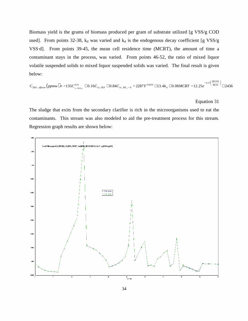
From points 1-7, permittivity differences in the group of (Farad/meter) were

varied. From points 8-14, the (g·hr/cm3·ton) was varied. From points 15-21, inlet

concentration of organics (Cin) (mg/L) was varied. From points 22-27, voltage (V) was varied.

From points 28-34, the exponential of conductivity divided by continuous phase permittivity

was varied. From points 35-41, the voltage field gradient, ∆E, in Volts, was varied. The final

resulting equation is shown below:

Equation 44

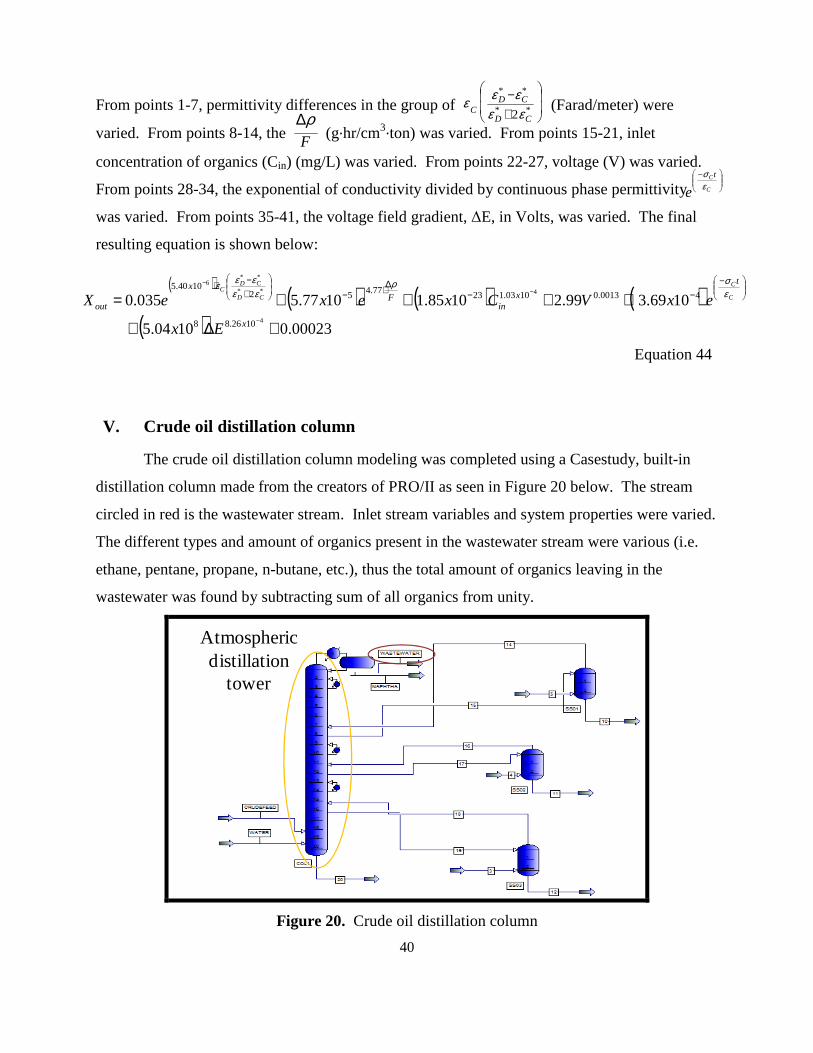
V. Crude oil distillation column

The crude oil distillation column modeling was completed using a Casestudy, built-in

distillation column made from the creators of PRO/II as seen in Figure 20 below. The stream

circled in red is the wastewater stream. Inlet stream variables and system properties were varied.

The different types and amount of organics present in the wastewater stream were various (i.e.

ethane, pentane, propane, n-butane, etc.), thus the total amount of organics leaving in the

wastewater was found by subtracting sum of all organics from unity.

Atmospheric distillation

tower

Figure 20. Crude oil distillation column

+−

**

**

2 CD

CDC εε

εεε

F

ρ∆

−

C

Ct

e εσ

( ) ( ) ( ) ( )( ) 00023.01004.5

1069.399.21085.11077.5035.04

4**

**6

1026.88

40013.01003.12377.4521040.5

+∆+

++++=−

−−

−−−

∆⋅−

+−⋅

x

t

xin

Fx

out

Ex

exVCxexeX C

C

CD

CDC ε

σρεε

εεε

41

The non-linear regression is shown below:

From points 1-50, crude feedrate, Fcrude (ton/hr), was varied. From points 51-150, steam

temperature, T (°F), was varied. From points 151-200, steam flowrate, Fsteam (ton/hr), was

varied. From points 201-250, efficiency (η) was varied. From points 251-257, the mass fraction

of organics in (Xin, organics) was varied. The resulting equation is shown below:

( )( ) ( ) 686.0719.0472.0135.0014.01088.110202.2

103250.0834.0419.1298.1606.0113.0234557.047

523456,

+⋅−⋅+⋅−⋅+++

−⋅−⋅+⋅−⋅+⋅−⋅=−−

−

ininininsteam

crudeoldout

xxxxFxTx

Fxx ηηηηηη

Equation 45

42

Comparison of concentration models with simulation results As is obvious from descriptions of how the equations were developed, the models are

linear in the sense that they were made by varying only one parameter at a time (for instance,

pressure was varied for 10 points, temperature for 10 poitns, flowrate for 10 points, etc.) Effects

between parameters were not considered (like how temperature would realistically change with

pressure) and this was hypothesized to introduce differences between real, simulated results and

those predicted from the theoretical, developed equations. To check for differences, inlet stream

parameters and system properties were randomly varied and 15 points were generated using the

simulation program and these results were compared to those predicted from the theoretical

equations. A correction equation was then applied to any model with a percent error of greater

than 5%, as this would be a difference of ~1-2 ppm (an acceptable difference).

%100% ×−

=resultlTheoretica

resultltheoreticaresultActualerror Equation 46

An example of a table generated is shown in Tables 6-7 below for the activated sludge system.

The % error was found to be at most ~3%.

Cin,TBOD5 (mg/L) Cin,TKN (mg/L) Cin, NH3-N (mg/L) Y (mg VSS/mg SBOD5) kD (d-1) MCRT (d) MLVSS/MLSS Cout, TKN (ppm)

Run 1 220 40 25 0.65 0.05 8 0.75 27.3

Run 2 220 85 50 0.65 0.05 8 0.75 55.4

Run 3 400 70 40 0.65 0.05 8 0.75 43

Run 4 200 70 40 0.4 0.1 5 0.75 49

Run 5 300 65 30 0.6 0.2 7 0.6 36.8

Run 6 110 30 12 0.3 0.09 3 0.55 20.8

Run 7 275 50 45 0.8 0.3 4 0.55 45.6

Run 8 275 50 25 0.65 0.15 8 0.4 29.2

Run 9 220 45 35 0.7 0.15 8 0.7 37.1

Run 10 200 70 50 0.65 0.3 10 0.3 54

Run 11 350 85 30 0.5 0.05 5 0.75 39.1

Run 12 325 85 25 0.8 0.25 8 0.8 36.5

Run 13 220 100 25 0.55 0.08 6 0.5 37.8

Run 14 300 35 30 0.65 0.05 7 0.5 30.4

Run 15 285 55 20 0.6 0.07 5 0.75 25.9

From Simulation (Steady )

Table 6. Simulated results from Steady by randomly varying variables that affect outlet concentration

Cin,TBOD5 (mg/L) Cin,TKN (mg/L) Cin, NH3-N (mg/L) Y (mg VSS/mg SBOD5) kD (d-1) MCRT (d) MLVSS/MLSS Cout, TKN (ppm)

Run 1 220 40 25 0.65 0.05 8 0.75 27.78433656

Run 2 220 85 50 0.65 0.05 8 0.75 55.98433656

Run 3 400 70 40 0.65 0.05 8 0.75 44.32997909

Run 4 200 70 40 0.4 0.1 5 0.75 48.6319467

Run 5 300 65 30 0.6 0.2 7 0.6 37.53360999

Run 6 110 30 12 0.3 0.09 3 0.55 20.41721864

Run 7 275 50 45 0.8 0.3 4 0.55 47.10733691

Run 8 275 50 25 0.65 0.15 8 0.4 29.41451499

Run 9 220 45 35 0.7 0.15 8 0.7 37.74815131

Run 10 200 70 50 0.65 0.3 10 0.3 55.93760778

Run 11 350 85 30 0.5 0.05 5 0.75 39.83904217

Run 12 325 85 25 0.8 0.25 8 0.8 36.00782756

Run 13 220 100 25 0.55 0.08 6 0.5 37.91973565

Run 14 300 35 30 0.65 0.05 7 0.5 29.96312713

Run 15 285 55 20 0.6 0.07 5 0.75 26.11839694

From Equation

Table 7. Predicted results from Steady by randomly varying variables that affect outlet concentration

43

The corresponding % error between each simulated and theoretical result is shown in Table 8.

The greatest % error is highlighted in yellow.

Cout, TKN (ppm) SIMULATION Cout, TKN (ppm) THEORETICAL % Error

27.3 27.78433656 1.774126584

55.4 55.98433656 1.054759129

43 44.32997909 3.092974631

49 48.6319467 0.75112918

36.8 37.53360999 1.99350542

20.8 20.41721864 1.840294983

45.6 47.10733691 3.30556339

29.2 29.41451499 0.734640393

37.1 37.74815131 1.747038569

54 55.93760778 3.58816255

39.1 39.83904217 1.890133416

36.5 36.00782756 1.348417653

37.8 37.91973565 0.316760976

30.4 29.96312713 1.437081801

25.9 26.11839694 0.843231418 Table 8. % error between simulation and theoretical results

The maximum % error was 3.59 %. As this is under 5%, the equation was regarded as

acceptable in predicting outlet concentrations. This same procedure was followed for the other

equations developed through a simulation program (Mathcad, PRO/II). The results are shown

below:

Water-using unit Error

H2S Stripper ± 38%

NH3 Stripper ± 31%

Crude oil distillation ± 5%

Biological Treatment ± 3%

Table 9. % Error for water-using units between simulated and theoretical equations

The crude oil distillation and biological treatment produced acceptable ranges for error, while the

H2S stripper and the NH3 stripper produced errors on the magnitude of ~30-40%. Thus, a

correction equation was developed to account for these differences and to try to equate the

44

equation result with the simulated result. As the H2S stripper always produced concentrations

less than the maximum outlet concentration of the Chevron Wastewater Treatment plant (5 ppm),

no correction equation was made. The ammonia stripper results are shown in Figure 21. The

correction equation is found to be y = 0.9392x+ 4.1579, where “x” is the result predicted from

the equation and “y” is the result found from the simulation program. The coefficient of

determination was found to be R2 = 0.6289. It’s clear that an applied linear regression did not

provide the best fit between simulated and predicted results. If any differences exist between

actual data from a refinery and predicted results, neglecting effects between stream variables

whilst developing models for the regeneration processes could be the source of error.

y = 0.9392x + 4.1579R² = 0.6289

0

5

10

15

20

25

30

35

40

0 5 10 15 20 25 30

Co

ut,

re

al (

pp

m)

Cout, equation (ppm)

NH3 Stripper

Figure 21. Correction equation for NH3 Stripper

45

Equipment Cost models

I. API separator

The majority of the costs that go into purchasing an API separator are the costs of the

material being used. Therefore, equipment cost will be a function primarily of the separator

volume. All that needs to be done are simple multiplications involving properties of the material

chosen to build the reactor. Stainless steel will be chosen as the API separator material because

it is durable and resistant to corrosionxxiv. The final equation is based off of density, volume, and

price of steel. A full derivation is shown in Appendix II.

( )305.6539 mVCost ⋅= Equation 47

II. Chevron Wastewater Treatment

Equipment costs for a Chevron Wastewater Treatment (CWWT) plant are dependent on

the number of trays, feedrate, vertical height of the columns, reboil ratio, materials cost, and

density difference between the passing streams. Since the CWWT plant consists of two stripping

columns, the equipment cost for one will be dependent on the same parameters as the other.

Basically, the diameter of the column was first solved for in terms of feedrate and the Souders

and Brown factor, which is a function of the density difference between passing streams.

Standard tray spacing for large-diameter columns are generally either 0.46 or 0.61 mxxv. 0.61

meter tray spacing was chosen in this study. The final result of equipment cost for a CWWT is

shown in Equation 27. A full derivation of the CWWT plant equipment costs is shown in

Appendix II.

( ) 421934.67474234

12

14

1195.0ln071.0

12.1

+⋅+=∆+

∆⋅∆− ρρρ RBR

F

eNHCostEquipment

Equation 48

III. Biological Treatment (Activated Sludge)

As mentioned before, an activated sludge system is the most common biological

treatment type. The system consists of an aeration tank where air is bubbled through the tank

wastewater followed by a settling tank where cellular material is removed by gravitational

46

settling. The aeration tank was modeled as an ideal CSTR. The turbulent conditions created by

the high flow rate air stream establish a perfect mixing environment. Equipment cost for the

secondary clarifier (settling tank) was found to be dependent on reactor size (m3), inlet flow rate

(ton/hr), and inlet concentration (ppm). A full derivation is shown in Appendix II.

( ) ( ) ( )( )[ ] F

orgCin

orgCinFmV ⋅+

+−⋅−⋅⋅=⋅= 019,866

001.0100,1.0

,10048.646183$CostEquipment 3

Equation 49

where ( )

( ) ForgCin

orgCinFV ⋅+

+−−⋅⋅≥ 9464

01.0100,

,10065.70 Equation 50

IV. Reverse Osmosis

The cost of the reverse osmosis was computed based on the most significant equipment

costs associated with the plant in the industry. These are the cost of the membrane replacement,

which has to be done frequently to avoid fouling and reduce efficiency and the pump cost. The

equation governing this cost was found to be:

⋅∆⋅+⋅⋅=

ηFP

NAyr

C 25.8053180$

ost Equipment Equation 51

where A: area per membrane

N: number of membrane used

F: flow rate to the process

V. Activated Carbon Adsorption

As a result of the adsorption being a fixed bed, the basic cost of the process was the cost

of regeneration of the bed after saturation. This cost of the fixed bed adsorber depends on the

capacity of the bed based on the feed concentration of the wastewater and given the equation:

QCtEquipment F7200$($)cos = Equation 52

47

Mathematical Programming Results General Algebraic Modeling System (GAMS)

The GAMS mathematical modeling program was used to optimize the placement and size

of the water streams in an oil refinery setting. Using the mixed integer program (MIP) and the

relaxed mixed integer program (rMIP) to solve the linear portions of the model as well as the

mixed integer non-linear program (MINLP) to solve the non-linear portions, we were able to

employ the CPLEX and DICOPT solvers to optimize the water regeneration system.

Figure 22. GAMS Program Screenshot

We optimized the system of equations based on two different objective functions, cost

and consumption:

• Cost = Annual Operation Cost + Annual Fixed Cost

• Consumption = Freshwater to water-using units + Freshwater to regeneration units

With these two objective functions, we set the output to give the lowest total annualized cost or

the lowest annual amount of freshwater consumed.

Past models of water regeneration processes made assumptions for the outlet

concentrations coming out of the water-using units and the regeneration processes. Assumptions

such as a fixed outlet concentration or a fixed unit efficiency caused previous models to provide

48

less than ideal results. With the modeled outlet concentrations mentioned in the first part of this

report, we are able to find more realistic results spanning a wider range of operating conditions.

With these more realistic results, a more confident conclusion can be reached on the economic

and environmental impact of utilizing the regeneration process model.

Results

The GAMS model that was created provided over 400,000 non-zero terms with over

1,200 non-linear, non-zero terms. The model took anywhere from one to five hours to run for

each simulation and read and processed over 17,000 lines of code. The output of the model

provided stream by stream data linking the freshwater source, water-using units, regeneration

processes, and water disposal sites all together. An example of the output data is shown in the

appendix. The program was run with only the regeneration processes containing outlet

concentration models. The water-using units will be added to the program at a later date. With

the model standing as it is now though, the process flow diagram of the refinery’s water using

units changed from a traditional flow like this:

Figure 23. Traditional Water Regeneration

to a new output where streams can flow back and forth from regeneration processes to water-

using units and back in the most efficient manner. An example of this new output is shown

below:

49

Figure 24. Optimized Water Regeneration

with this schematic, the following contaminant concentrations were cleaned using the

regeneration processes:

By including the modeled outlet concentrations of the regeneration processes into our

mathematical model, we provided more realistic results to conclude an expected cost of

$950,000 (instead of $1,220,000 as seen with the fixed outlet concentration model) and a water

consumption of 31 tons/hour (instead of 33 tons/hour). We obtained these results by setting

Contaminant Stream Concentration Reduction (ppm) Salts Organics H2S Ammonia

621.18 7153.77 27.23 18.61

50

constraints of 250 tons/hour as the maximum stream flow rate and a contaminant outlet limit of

20, 50, 5, and 30 ppm for salts, organics, H2S, and ammonia respectively. These model results

might differ minimally between fixed outlet concentrations and modeled outlet concentrations,

but the improved reliability and confidence provides a more usable program for any user who

might find it useful. Further tables indicating water stream placement (i.e. flow rate to and from

water-using and regeneration processes in ton/hr) are seen in Appendix III.

Conclusions This study focused on deriving original correlations for predicting wastewater

contaminant levels from water treatment and a few water-using units in petroleum refineries.

While there is no exact model that exists to find contaminant levels, non-linear regression can be

used to approximate a highly accurate answer (with determination coefficients in the range of

~0.99). However, since developed models were found by varying one parameter at a time, non-

linear models (i.e. accounting for how pressure might be related to temperature simultaneously)

of the outlet concentration of contaminants provide a more accurate model to represent refinery

waste water generation. Of course, all of the procedures aforementioned are performed based on

the assumption that the simulation method used is highly accurate. For the sake of this study,

which uses programs like PRO/II and Mathcad to generate points for a guessed model, it will be

assumed that errors are at a minimum within the system. Other simulation programs like

Aspen’s HYSYS could be used to check the accuracy of PRO/II runs, if made available to the

student. Also, comparing actual data from a petroleum refinery with theoretical model results

would ensure that the guessed models in this study are at least close to predicted values, if not

entirely incorrect. Once again though, availability is the dilemma at hand, as the information

needed to compare could be closely guarded and perhaps laden with legal consequences. As

government regulations are becoming increasingly strict in laws regarding treated wastewater, it

is, in effect, becoming important to develop more accurate models. Accurate predictions of

treated water streams and obeying the government standards set for these contaminant levels not

only guarantees a trouble-free work environment, but also promotes a safe and healthy living

environment. A final conclusion is that equipment costs of the water regeneration processes are

a function of inlet concentrations and flow rates, as well as design parameters.

51

Recommendations The crux of wastewater management lies in the optimization of wastewater and

freshwater streams. Thus, as optimization models increase in accuracy, the accuracy of

corresponding stream placement and flowrates increase. Recommendations for future work in

the continuing water management problem include:

• Modeling of the vacuum distillation column, hydrotreatment unit, and Merox I

sweetening unit

• More accurate modeling of operating costs for the regeneration processes

• Implement all newly-found models in GAMS file (mathematical model)

• Expand the scope of the project to include other industrial cases where water

is used to treat contaminants, e.g. a tricresyl phosphate process or a paper mill

process

• Derive an economic plan for refinery wastewater system (including costs of

piping, costs of process units, location and prices of pumps, salaries, etc.)

• Investigate water treatment and water-using units for countries other than the

U.S., like Canada or Mexico

o Find out if the water treatment and water-using units are similar to

those used in the U.S.

o What are the permitted drinking water contaminant levels in that

country? Are they similar to the U.S.? If so, are large oil companies

abiding by these laws?

o Are industries really following government guidelines? Is the

government even setting a guideline? If not, could this be the reason

why so many oil companies are willing to export their business to

countries outside of the U.S. so they don’t have to adhere to strict

water laws? What kind of money could be saved if water treatment

processes were used at a bare minimum?

52

References Chemical and Physical Information. Hydrogen Sulfide. Date accessed: 7 April 2009.

<http://www.atsdr.cdc.gov/toxprofiles/tp114-c4.pdf>. 2006.

Date accessed: 10 April 2009. Water Quality, Ammonia. <http://www.eerc.und.nodak.edu/

Watman/FMRiver/PPTV/ammonia.asp>.

Gammelgard, P. N. Water Pollution Control in Petroleum Refineries in the United States.

American Petroleum Institute.

Liptak, Bela G., and Liu, David H. F. Environmental Engineers’ Handbook. 2nd Ed. CRC

Press. 1999.

Newson, Malcolm David. Land, Water and Development. Routledge. 1997. Sams, Gary W., and Warren, Kenneth, W. New Methods of Application of Electrostatic Fields.

©NATCO Group. 2003.

Saudi Arabian Water Environment Association (SAWEA). Wastewater Treatment, Treatment

Options & Key Design Issues. Siemens Business.

Seader, J.D., and Henley, Ernest J. Separation Process Principles. 2nd Ed. John Wiley & Sons,

Inc. 2006.

Spirkin, V. G., Gil’mutdinov, Sh. K., and Akhmetshin, E. A. Evaluation of Oil Lubricity in the

Presence of Hydrogen Sulfide. Ufa Petroleum Institute. 1993.

53

Appendix I API Separator table:

Mole fraction retained

L (m) 20 24 28 32 36 40 44 48 52

W (m) 3.5 3.5 3.5 3.5 3.5 3.5 3.5 3.5 3.5

H (m) 1.5 1.5 1.5 1.5 1.5 1.5 1.5 1.5 1.5

V (m3) 105 126 147 168 189 210 231 252 273

Height at which particle enters Flow (m3/s) Flow (ton/hr)

0.01 0.0010 3.961270121 0.962 0.965 0.968 0.970 0.971 0.973 0.974 0.975 0.976

0.01 0.0051 20.20247762 0.911 0.919 0.925 0.930 0.934 0.938 0.941 0.943 0.946

0.01 0.0101 40.00882822 0.874 0.885 0.894 0.901 0.907 0.912 0.916 0.920 0.923

0.01 0.0151 59.81517883 0.845 0.859 0.870 0.878 0.885 0.891 0.897 0.901 0.905

0.01 0.0201 79.62152944 0.821 0.837 0.849 0.859 0.867 0.874 0.880 0.886 0.890

0.01 0.0251 99.42788004 0.801 0.818 0.831 0.842 0.851 0.859 0.866 0.872 0.877

0.01 0.0301 119.2342307 0.782 0.801 0.815 0.827 0.837 0.846 0.853 0.859 0.865

0.01 0.0351 139.0405813 0.765 0.785 0.801 0.813 0.824 0.833 0.841 0.848 0.854

0.01 0.0401 158.8469319 0.750 0.771 0.787 0.801 0.812 0.822 0.830 0.837 0.844

0.01 0.0451 178.6532825 0.736 0.758 0.775 0.789 0.801 0.811 0.820 0.827 0.834

0.01 0.0501 198.4596331 0.723 0.745 0.763 0.778 0.790 0.801 0.810 0.818 0.825

0.01 0.0551 218.2659837 0.711 0.734 0.752 0.767 0.780 0.791 0.801 0.809 0.817

0.3 0.0010 3.961270121 0.966 0.969 0.971 0.973 0.974 0.976 0.977 0.978 0.979

0.3 0.0051 20.20247762 0.921 0.928 0.933 0.938 0.941 0.944 0.947 0.949 0.951

0.3 0.0101 40.00882822 0.887 0.897 0.905 0.911 0.917 0.921 0.925 0.928 0.931

0.3 0.0151 59.81517883 0.861 0.874 0.883 0.891 0.897 0.903 0.908 0.912 0.915

0.3 0.0201 79.62152944 0.840 0.854 0.865 0.874 0.881 0.888 0.893 0.898 0.902

0.3 0.0251 99.42788004 0.821 0.837 0.849 0.859 0.867 0.874 0.880 0.885 0.890

0.3 0.0301 119.2342307 0.804 0.821 0.834 0.845 0.854 0.862 0.868 0.874 0.879

0.3 0.0351 139.0405813 0.789 0.807 0.821 0.833 0.842 0.850 0.857 0.864 0.869

0.3 0.0401 158.8469319 0.774 0.794 0.809 0.821 0.831 0.840 0.848 0.854 0.860

0.3 0.0451 178.6532825 0.761 0.781 0.797 0.810 0.821 0.830 0.838 0.845 0.851

0.3 0.0501 198.4596331 0.749 0.770 0.787 0.800 0.811 0.821 0.829 0.837 0.843

0.3 0.0551 218.2659837 0.738 0.759 0.776 0.791 0.802 0.812 0.821 0.829 0.835

0.5 0.0010 3.961270121 0.969 0.971 0.974 0.975 0.977 0.978 0.979 0.980 0.981

0.5 0.0051 20.20247762 0.928 0.934 0.939 0.943 0.947 0.949 0.952 0.954 0.956

0.5 0.0101 40.00882822 0.897 0.906 0.914 0.919 0.924 0.928 0.932 0.935 0.937

0.5 0.0151 59.81517883 0.874 0.885 0.894 0.901 0.907 0.912 0.916 0.920 0.923

0.5 0.0201 79.62152944 0.854 0.867 0.877 0.885 0.892 0.898 0.902 0.907 0.911

0.5 0.0251 99.42788004 0.837 0.851 0.862 0.871 0.879 0.885 0.891 0.895 0.900

0.5 0.0301 119.2342307 0.821 0.837 0.849 0.859 0.867 0.874 0.880 0.885 0.890

0.5 0.0351 139.0405813 0.807 0.823 0.837 0.847 0.856 0.864 0.870 0.876 0.881

0.5 0.0401 158.8469319 0.794 0.811 0.825 0.837 0.846 0.854 0.861 0.867 0.872

0.5 0.0451 178.6532825 0.781 0.800 0.815 0.827 0.837 0.845 0.852 0.859 0.864

0.5 0.0501 198.4596331 0.770 0.789 0.805 0.817 0.828 0.837 0.844 0.851 0.857

0.5 0.0551 218.2659837 0.759 0.780 0.795 0.808 0.819 0.829 0.837 0.844 0.850

0.75 0.0010 3.961270121 0.973 0.975 0.977 0.979 0.980 0.981 0.982 0.983 0.983

0.75 0.0051 20.20247762 0.938 0.943 0.948 0.951 0.954 0.956 0.958 0.960 0.962

0.75 0.0101 40.00882822 0.911 0.919 0.926 0.930 0.935 0.938 0.941 0.944 0.946

0.75 0.0151 59.81517883 0.891 0.901 0.908 0.914 0.920 0.924 0.927 0.931 0.933

0.75 0.0201 79.62152944 0.874 0.885 0.894 0.901 0.907 0.912 0.916 0.920 0.923

0.75 0.0251 99.42788004 0.859 0.871 0.881 0.889 0.895 0.901 0.906 0.910 0.913

0.75 0.0301 119.2342307 0.845 0.859 0.869 0.878 0.885 0.891 0.896 0.901 0.905

0.75 0.0351 139.0405813 0.833 0.847 0.859 0.868 0.876 0.882 0.888 0.893 0.897

0.75 0.0401 158.8469319 0.821 0.837 0.849 0.859 0.867 0.874 0.880 0.885 0.890

0.75 0.0451 178.6532825 0.810 0.827 0.840 0.850 0.859 0.866 0.873 0.878 0.883

0.75 0.0501 198.4596331 0.800 0.817 0.831 0.842 0.851 0.859 0.866 0.871 0.877

0.75 0.0551 218.2659837 0.791 0.808 0.823 0.834 0.844 0.852 0.859 0.865 0.870

1 0.0010 3.961270121 0.978 0.980 0.981 0.983 0.984 0.984 0.985 0.986 0.986

1 0.0051 20.20247762 0.949 0.954 0.957 0.960 0.963 0.964 0.966 0.968 0.969

1 0.0101 40.00882822 0.928 0.935 0.940 0.944 0.947 0.950 0.952 0.954 0.956

1 0.0151 59.81517883 0.912 0.920 0.926 0.931 0.935 0.938 0.941 0.944 0.946

1 0.0201 79.62152944 0.898 0.907 0.914 0.920 0.924 0.928 0.932 0.935 0.937

1 0.0251 99.42788004 0.885 0.895 0.903 0.910 0.915 0.920 0.923 0.927 0.930

1 0.0301 119.2342307 0.874 0.885 0.894 0.901 0.907 0.912 0.916 0.920 0.923

1 0.0351 139.0405813 0.864 0.876 0.885 0.893 0.899 0.904 0.909 0.913 0.917

1 0.0401 158.8469319 0.854 0.867 0.877 0.885 0.892 0.898 0.903 0.907 0.911

1 0.0451 178.6532825 0.845 0.859 0.870 0.878 0.885 0.891 0.897 0.901 0.905

1 0.0501 198.4596331 0.837 0.851 0.862 0.871 0.879 0.885 0.891 0.896 0.900

1 0.0551 218.2659837 0.829 0.844 0.855 0.865 0.873 0.880 0.885 0.890 0.895

1.25 0.0010 3.961270121 0.984 0.986 0.987 0.988 0.988 0.989 0.990 0.990 0.990

1.25 0.0051 20.20247762 0.964 0.968 0.970 0.972 0.974 0.975 0.976 0.977 0.978

1.25 0.0101 40.00882822 0.950 0.954 0.958 0.960 0.963 0.965 0.966 0.968 0.969

1.25 0.0151 59.81517883 0.938 0.944 0.948 0.951 0.954 0.957 0.959 0.960 0.962

1.25 0.0201 79.62152944 0.928 0.935 0.940 0.944 0.947 0.950 0.952 0.954 0.956

1.25 0.0251 99.42788004 0.920 0.927 0.932 0.937 0.941 0.944 0.946 0.949 0.951

1.25 0.0301 119.2342307 0.912 0.920 0.926 0.931 0.935 0.938 0.941 0.944 0.946

1.25 0.0351 139.0405813 0.904 0.913 0.920 0.925 0.929 0.933 0.936 0.939 0.942

1.25 0.0401 158.8469319 0.898 0.907 0.914 0.920 0.924 0.928 0.932 0.935 0.937

1.25 0.0451 178.6532825 0.891 0.901 0.909 0.915 0.920 0.924 0.928 0.931 0.934

1.25 0.0501 198.4596331 0.885 0.896 0.904 0.910 0.915 0.920 0.924 0.927 0.930

1.25 0.0551 218.2659837 0.880 0.890 0.899 0.905 0.911 0.916 0.920 0.923 0.926

1.49 0.0010 3.961270121 0.997 0.997 0.997 0.998 0.998 0.998 0.998 0.998 0.998

1.49 0.0051 20.20247762 0.993 0.994 0.994 0.994 0.995 0.995 0.995 0.996 0.996

1.49 0.0101 40.00882822 0.990 0.991 0.992 0.992 0.993 0.993 0.993 0.994 0.994

1.49 0.0151 59.81517883 0.988 0.989 0.990 0.990 0.991 0.991 0.992 0.992 0.993

1.49 0.0201 79.62152944 0.986 0.987 0.988 0.989 0.990 0.990 0.991 0.991 0.991

1.49 0.0251 99.42788004 0.984 0.986 0.987 0.988 0.988 0.989 0.990 0.990 0.990

1.49 0.0301 119.2342307 0.983 0.984 0.986 0.987 0.987 0.988 0.989 0.989 0.989

1.49 0.0351 139.0405813 0.982 0.983 0.984 0.985 0.986 0.987 0.988 0.988 0.989

1.49 0.0401 158.8469319 0.980 0.982 0.983 0.984 0.985 0.986 0.987 0.987 0.988

1.49 0.0451 178.6532825 0.979 0.981 0.982 0.983 0.984 0.985 0.986 0.987 0.987

1.49 0.0501 198.4596331 0.978 0.980 0.981 0.983 0.984 0.984 0.985 0.986 0.986

1.49 0.0551 218.2659837 0.977 0.979 0.980 0.982 0.983 0.984 0.984 0.985 0.986

54

Polymath results for activated sludge: POLYMATH Results No Title 03-02-2009 Nonlinear regression (L-M) Model: TKNeffluent = a*(TBOD5^b)+c*TKN+e*NH3N+g*(Y^i)+j*kd+m*MCRT+(o*MLVSStoMLSS*MLVSStoMLSS)+(p*MLVSStoMLSS)+d Variable Ini guess Value 95% confidence a 35 20.033392 0.2483401 b -0.04 -0.1381159 0.0022601 c 0.16 0.0055365 0.0021003 e 0.843 0.4414261 0.0049 g 26 15.213166 0.1693005 i -0.11 0.8397723 0.0251757 j 13.4 -69.166537 1.3530784 m 0.083 -0.4107851 0.0080561 o 25 7.3439867 0.2195136 p 0.123 -13.176989 0.1637615 d 1300 1290.1729 0.1163555 Nonlinear regression settings Max # iterations = 300 Precision R^2 = -3.233E+04 R^2adj = -3.921E+04 Rmsd = 167.96354 Variance = 2.019E+06 General Sample size = 58 # Model vars = 11 # Indep vars = 7 # Iterations = 22

55

Polymath report for sludge in activated sludge: POLYMATH Results No Title 02-25-2009 Nonlinear regression (L-M) Model: TKNsludge = a*(TBOD5^b)+c*TKN+e*NH3N+g*(Y^i)+j*kd+m*MCRT+(o*MLVSStoMLSS*MLVSStoMLSS)+(p*MLVSStoMLSS)+(q*mgBODtomgVSS)+d Variable Ini guess Value 95% confidence a 2.447E+05 3.436E+05 6.195E+05 b -0.989 -1.0566498 0.3699678 c 77.9 77.885427 0.2837419 e -77 -77.035544 1.3641259 g 780 762.48543 74.635933 i -0.99 -0.998504 0.03776 j 6673 6684.5207 127.00663 m 42 41.789081 0.7679007 o -1798 -99.853572 307.24985 p 1829 1021.5736 253.5563 q -83.4 -75.891695 97.216543 d 4598 -3663.6664 255.4147 Nonlinear regression settings Max # iterations = 300 Precision R^2 = 0.9998816 R^2adj = 0.9998533 Rmsd = 3.3082243 Variance = 800.36492 General Sample size = 58 # Model vars = 12 # Indep vars = 8 # Iterations = 27

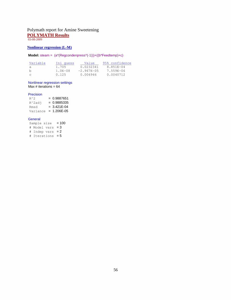
56

Polymath report for Amine Sweetening POLYMATH Results 03-08-2009 Nonlinear regression (L-M) Model: steam = (a*(Regcondenpress^(-1)))+((b*Feedtemp)+c) Variable Ini guess Value 95% confidence a 1.705 0.0232341 8.851E-04 b 1.0E-08 -2.967E-05 7.559E-06 c 0.125 0.006946 0.0040712 Nonlinear regression settings Max # iterations = 64 Precision R^2 = 0.9887651 R^2adj = 0.9885335 Rmsd = 3.421E-04 Variance = 1.206E-05 General Sample size = 100 # Model vars = 3 # Indep vars = 2 # Iterations = 5

57

Polymath results for H2S Stripper: POLYMATH Results No Title 04-20-2009 Nonlinear regression (L-M) Model: CoutH2S = a*exp(b*CinNH3)+c*exp(d*Temp)+e*(Efficiency^f)+g*(CinH2S^2)+(h*CinH2S)+i*(Numberoftrays^j)+k Variable Ini guess Value 95% confidence a 2.0E-06 0.0023514 6.18E-04 b 0.7648 0.0792118 0.0565716 c 3.0E-06 -1.0002578 0.3104719 d 0.0142 -0.0385425 0.0020614 e 3.0E-05 -0.0143649 7.966E-04 f -0.908 -0.137697 0.1722801 g 1.0E-06 0.0112059 2.959E-05 h -2.0E-06 0.0012207 1.618E-04 i 5244 2.17E+04 24.371227 j -7.377 -7.0772926 0.0010207 k 9.0E-06 0.015824 8.152E-05 Nonlinear regression settings Max # iterations = 300 Precision R^2 = 0.9994561 R^2adj = 0.9994201 Rmsd = 0.0013088 Variance = 2.977E-04 General Sample size = 162 # Model vars = 11 # Indep vars = 5 # Iterations = 71

58

Polymath results for NH3 Stripper: POLYMATH Report No Title Nonlinear Regression (L-M) 28-Apr-2009 Model: CoutNH3 = a*(Feedrate^2)+b*Feedrate+c*CinNH3+d*exp(Numberoftrays*e)+f*exp(g*Temp)+h*RFR+i*(Pressure^j)+k*(Efficiency^2)+l*Efficiency+m*(CinH2S^n)+o

Variable Initial guess Value 95% confidence

a 0.0006 0.0006762 3.554E-06

b 0.0106 -0.0064736 9.96E-05

c 0.0306 -0.056633 0.0006159

d 9106.6 1.546E+04 0.4341984

e -0.824 -0.6966562 5.606E-06

f 7.0E-05 8.069E-05 3.885E-09

g 0.0247 0.0250764 8.003E-08

h 0.0069 0.0612676 0.0005577

i 4.481E+04 -4.436E+06 2.257E+04

j -2.572 -2.940971 0.0009171

k 0.1883 -0.5269187 0.0029861

l -0.3277 -0.7517399 0.0023763

m 0.041 7.1049645 7.0639645

n -0.065 0.470095 0.535095

o 0.322 0.237672 0.0018679

Nonlinear regression settings Max # iterations = 300 Precision R^2 0.9148893

R^2adj 0.8817907

Rmsd 2.460408

Variance 437.3733

General Sample size 51

Model vars 15

Indep vars 8

Iterations 18

59

Source data points and calculated data points

Feedrate CinNH3 Numberoftrays Temp RFR Pressure Efficiency CinH2S CoutNH3 CoutNH3 calc

Delta CoutNH3

1 5 3 15 250 3 250 0.8 5 0.00642 -0.6054326 0.6118526

2 10 3 15 250 3 250 0.8 5 0.0752 -0.5870836 0.6622836

3 15 3 15 250 3 250 0.8 5 0.0924 -0.5349234 0.6273234

4 20 3 15 250 3 250 0.8 5 0.124 -0.448952 0.572952

5 25 3 15 250 3 250 0.8 5 0.187 -0.3291694 0.5161694

6 30 3 15 250 3 250 0.8 5 0.277 -0.1755756 0.4525756

7 35 3 15 250 3 250 0.8 5 0.406 0.0118294 0.3941706

8 40 3 15 250 3 250 0.8 5 0.597 0.2330456 0.3639544

9 42 3 15 250 3 250 0.8 5 0.697 0.3309992 0.3660008

10 43 3 15 250 3 250 0.8 5 0.755 0.3820047 0.3729953

11 15 0.3 15 250 3 250 0.8 5 0.00541 -0.3820144 0.3874244

12 15 0.75 15 250 3 250 0.8 5 0.0153 -0.4074992 0.4227992

13 15 1 15 250 3 250 0.8 5 0.0219 -0.4216575 0.4435575

14 15 1.5 15 250 3 250 0.8 5 0.0334 -0.449974 0.483374

15 15 2 15 250 3 250 0.8 5 0.0461 -0.4782904 0.5243904

16 15 2.5 15 250 3 250 0.8 5 0.061 -0.5066069 0.5676069

17 15 4 15 250 3 250 0.8 5 0.108 -0.5915564 0.6995564

18 15 5 15 250 3 250 0.8 5 0.143 -0.6481894 0.7911894

19 15 6 15 250 3 250 0.8 5 0.18 -0.7048223 0.8848223

20 15 3 5 250 3 250 0.8 5 350 473.8129 -123.8129

21 15 3 10 250 3 250 0.8 5 0.424 13.5967 -13.1727

22 15 3 20 250 3 250 0.8 5 0.00483 -0.9688562 0.9736862

23 15 3 25 250 3 250 0.8 5 0.00000242 -0.9821808 0.9821832

24 15 3 30 250 3 250 0.8 5 0.00000022 -0.9825899 0.9825901

25 15 3 15 200 3 250 0.8 5 0.0236 -0.5653663 0.5889663

26 15 3 15 300 3 250 0.8 5 0.0273 -0.4282608 0.4555608

27 15 3 15 400 3 250 0.8 5 1.8 1.254832 0.5451683

28 15 3 15 500 3 250 0.8 5 11.2 21.9163 -10.7163

29 15 3 15 600 3 250 0.8 5 265 275.5544 -10.55436

30 15 3 15 250 2 250 0.8 5 0.0658 -0.596191 0.661991

31 15 3 15 250 4 250 0.8 5 0.0503 -0.4736559 0.5239559

32 15 3 15 250 5 250 0.8 5 0.0399 -0.4123883 0.4522883

33 15 3 15 250 7 250 0.8 5 0.0283 -0.2898532 0.3181532

34 15 3 15 250 8 250 0.8 5 0.025 -0.2285856 0.2535856

35 15 3 15 250 3 300 0.8 5 0.0354 -0.3716959 0.4070959

36 15 3 15 250 3 400 0.8 5 0.00475 -0.2403553 0.2451053

37 15 3 15 250 3 500 0.8 5 0.00332 -0.1928509 0.1961709

60

38 15 3 15 250 3 600 0.8 5 0.00338 -0.1715953 0.1749753

39 15 3 15 250 3 700 0.8 5 0.00251 -0.1606753 0.1631853

40 15 3 15 250 3 750 0.8 5 0.00217 -0.1571789 0.1593489

41 15 3 15 250 3 800 0.8 5 0.00165 -0.154492 0.156142

42 15 3 15 250 3 250 0.4 5 0.0658 0.0186935 0.0471065

43 15 3 15 250 3 250 0.5 5 0.0503 -0.1039031 0.1542031

44 15 3 15 250 3 250 0.6 5 0.0399 -0.2370382 0.2769382

45 15 3 15 250 3 250 0.7 5 0.0283 -0.3807116 0.4090116

46 15 3 15 250 3 250 0.9 5 0.025 -0.6996736 0.7246736

47 15 3 15 250 3 250 0.8 0.5 0.0448 1.791348 -1.746548

48 15 3 15 250 3 250 0.8 1 0.0391 -0.4300377 0.4691377

49 15 3 15 250 3 250 0.8 2 0.0388 -0.5302663 0.5690663

50 15 3 15 250 3 250 0.8 6 0.0357 -0.5349673 0.5706673

51 15 3 15 250 3 250 0.8 10 0.0365 -0.5349987 0.5714987

61

Polymath results for crude oil distillation column: POLYMATH Report No Title Nonlinear Regression (L-M) 20-Apr-2009 Model: Xoutwater = a*Efficiency^6-b*Efficiency^5+c*Efficiency^4-d*Efficiency^3+e*Efficiency^2-f*Efficiency-g*Crudefeed+h*Steamtemp+i*Steamflow^j+k+l*(Xinorganics^4)+m*(Xinorganics^3)+n*(Xinorganics^2)+o*Xinorganics Variable Initial guess Value 95% confidence

a 0.1236 0.1129874 0.1295418

b 0.6655 0.6058456 0.684952

c 1.4344 1.297872 1.466419

d 1.5817 1.418556 1.622575

e 0.9411 0.8338002 0.9757995

f 0.2865 0.2497371 0.3015229

g 3.0E-05 2.992E-05 4.024E-07

h 1.0E-07 2.202E-07 3.411E-08

i 0.0174 0.0055334 0.0001881

j 0.4295 0.5565462 0.003919

k 1.7 0.7096117 0.3139925

l 0.0149 0.0143246 0.0101507

m -0.1402 -0.1353119 0.0970516

n 0.488 0.4716159 0.3442684

o -0.7433 -0.7189798 0.5370286

Nonlinear regression settings Max # iterations = 300 Precision R^2 0.999988

R^2adj 0.9999873

Rmsd 9.227E-06

Variance 2.324E-08

General Sample size 257

Model vars 15

Indep vars 5

Iterations 26

62

Source data points and calculated data points

Efficiency Crudefeed Steamtemp Steamflow Xinorganics Xoutwater Xoutwater calc Delta Xoutwater

1 0.4 6548.3 600 555 3 0.26486 0.2648542 5.751E-06

2 0.4 6553.3 600 555 3 0.26471 0.2647047 5.346E-06

3 0.4 6558.3 600 555 3 0.26456 0.2645551 4.942E-06

4 0.4 6563.3 600 555 3 0.26441 0.2644055 4.537E-06

5 0.4 6568.3 600 555 3 0.26425 0.2642559 -5.868E-06

6 0.4 6573.3 600 555 3 0.2641 0.2641063 -6.273E-06

7 0.4 6578.3 600 555 3 0.26395 0.2639567 -6.678E-06

8 0.4 6583.3 600 555 3 0.2638 0.2638071 -7.083E-06

9 0.4 6588.3 600 555 3 0.26365 0.2636575 -7.487E-06

10 0.4 6593.3 600 555 3 0.26349 0.2635079 -1.789E-05

11 0.4 6598.3 600 555 3 0.26334 0.2633583 -1.83E-05

12 0.4 6603.3 600 555 3 0.26319 0.2632087 -1.87E-05

13 0.4 6608.3 600 555 3 0.26304 0.2630591 -1.911E-05

14 0.4 6613.3 600 555 3 0.26289 0.2629095 -1.951E-05

15 0.4 6618.3 600 555 3 0.26274 0.2627599 -1.992E-05

16 0.4 6623.3 600 555 3 0.26259 0.2626103 -2.032E-05

17 0.4 6628.3 600 555 3 0.26244 0.2624607 -2.073E-05

18 0.4 6633.3 600 555 3 0.26229 0.2623111 -2.113E-05

19 0.4 6638.3 600 555 3 0.26214 0.2621615 -2.154E-05

20 0.4 6643.3 600 555 3 0.26199 0.2620119 -2.194E-05

21 0.4 6648.3 600 555 3 0.26184 0.2618623 -2.235E-05

22 0.4 6653.3 600 555 3 0.26169 0.2617128 -2.275E-05

23 0.4 6658.3 600 555 3 0.26154 0.2615632 -2.316E-05

24 0.4 6663.3 600 555 3 0.26139 0.2614136 -2.356E-05

25 0.4 6668.3 600 555 3 0.26124 0.261264 -2.396E-05

26 0.4 6673.3 600 555 3 0.26109 0.2611144 -2.437E-05

27 0.4 6678.3 600 555 3 0.26094 0.2609648 -2.477E-05

28 0.4 6683.3 600 555 3 0.26079 0.2608152 -2.518E-05

29 0.4 6688.3 600 555 3 0.26065 0.2606656 -1.558E-05

30 0.4 6693.3 600 555 3 0.2605 0.260516 -1.599E-05

31 0.4 6698.3 600 555 3 0.26035 0.2603664 -1.639E-05

32 0.4 6703.3 600 555 3 0.2602 0.2602168 -1.68E-05

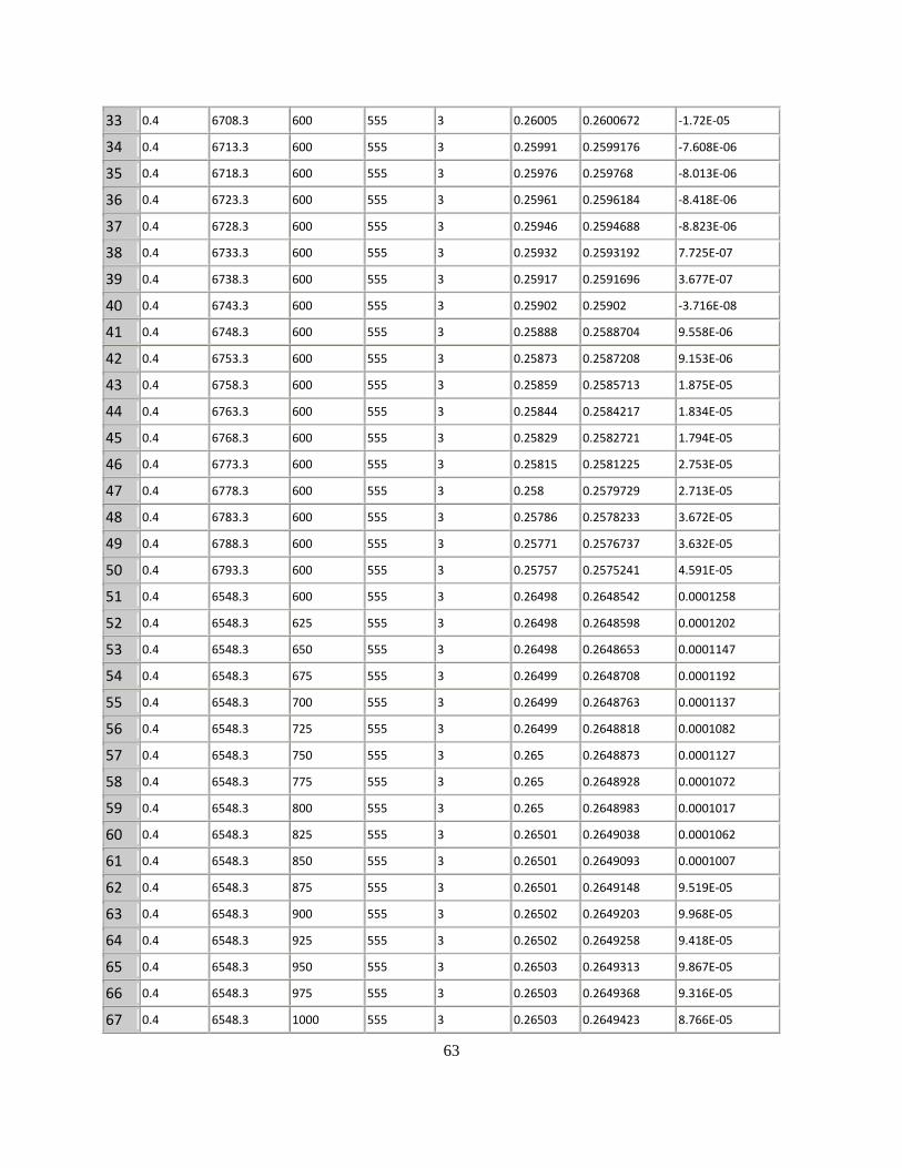
63

33 0.4 6708.3 600 555 3 0.26005 0.2600672 -1.72E-05

34 0.4 6713.3 600 555 3 0.25991 0.2599176 -7.608E-06

35 0.4 6718.3 600 555 3 0.25976 0.259768 -8.013E-06

36 0.4 6723.3 600 555 3 0.25961 0.2596184 -8.418E-06

37 0.4 6728.3 600 555 3 0.25946 0.2594688 -8.823E-06

38 0.4 6733.3 600 555 3 0.25932 0.2593192 7.725E-07

39 0.4 6738.3 600 555 3 0.25917 0.2591696 3.677E-07

40 0.4 6743.3 600 555 3 0.25902 0.25902 -3.716E-08

41 0.4 6748.3 600 555 3 0.25888 0.2588704 9.558E-06

42 0.4 6753.3 600 555 3 0.25873 0.2587208 9.153E-06

43 0.4 6758.3 600 555 3 0.25859 0.2585713 1.875E-05

44 0.4 6763.3 600 555 3 0.25844 0.2584217 1.834E-05

45 0.4 6768.3 600 555 3 0.25829 0.2582721 1.794E-05

46 0.4 6773.3 600 555 3 0.25815 0.2581225 2.753E-05

47 0.4 6778.3 600 555 3 0.258 0.2579729 2.713E-05

48 0.4 6783.3 600 555 3 0.25786 0.2578233 3.672E-05

49 0.4 6788.3 600 555 3 0.25771 0.2576737 3.632E-05

50 0.4 6793.3 600 555 3 0.25757 0.2575241 4.591E-05

51 0.4 6548.3 600 555 3 0.26498 0.2648542 0.0001258

52 0.4 6548.3 625 555 3 0.26498 0.2648598 0.0001202

53 0.4 6548.3 650 555 3 0.26498 0.2648653 0.0001147

54 0.4 6548.3 675 555 3 0.26499 0.2648708 0.0001192

55 0.4 6548.3 700 555 3 0.26499 0.2648763 0.0001137

56 0.4 6548.3 725 555 3 0.26499 0.2648818 0.0001082

57 0.4 6548.3 750 555 3 0.265 0.2648873 0.0001127

58 0.4 6548.3 775 555 3 0.265 0.2648928 0.0001072

59 0.4 6548.3 800 555 3 0.265 0.2648983 0.0001017

60 0.4 6548.3 825 555 3 0.26501 0.2649038 0.0001062

61 0.4 6548.3 850 555 3 0.26501 0.2649093 0.0001007

62 0.4 6548.3 875 555 3 0.26501 0.2649148 9.519E-05

63 0.4 6548.3 900 555 3 0.26502 0.2649203 9.968E-05

64 0.4 6548.3 925 555 3 0.26502 0.2649258 9.418E-05

65 0.4 6548.3 950 555 3 0.26503 0.2649313 9.867E-05

66 0.4 6548.3 975 555 3 0.26503 0.2649368 9.316E-05

67 0.4 6548.3 1000 555 3 0.26503 0.2649423 8.766E-05

64

68 0.4 6548.3 1025 555 3 0.26504 0.2649478 9.215E-05

69 0.4 6548.3 1050 555 3 0.26504 0.2649534 8.665E-05

70 0.4 6548.3 1075 555 3 0.26504 0.2649589 8.114E-05

71 0.4 6548.3 1100 555 3 0.26505 0.2649644 8.564E-05

72 0.4 6548.3 1125 555 3 0.26505 0.2649699 8.013E-05

73 0.4 6548.3 1150 555 3 0.26505 0.2649754 7.462E-05

74 0.4 6548.3 1175 555 3 0.26506 0.2649809 7.912E-05

75 0.4 6548.3 1200 555 3 0.26506 0.2649864 7.361E-05

76 0.4 6548.3 1225 555 3 0.26506 0.2649919 6.811E-05

77 0.4 6548.3 1250 555 3 0.26507 0.2649974 7.26E-05

78 0.4 6548.3 1275 555 3 0.26507 0.2650029 6.71E-05

79 0.4 6548.3 1300 555 3 0.26508 0.2650084 7.159E-05

80 0.4 6548.3 1325 555 3 0.26508 0.2650139 6.608E-05

81 0.4 6548.3 1350 555 3 0.26508 0.2650194 6.058E-05

82 0.4 6548.3 1375 555 3 0.26509 0.2650249 6.507E-05

83 0.4 6548.3 1400 555 3 0.26509 0.2650304 5.957E-05

84 0.4 6548.3 1425 555 3 0.26509 0.2650359 5.406E-05

85 0.4 6548.3 1450 555 3 0.2651 0.2650414 5.856E-05

86 0.4 6548.3 1475 555 3 0.2651 0.265047 5.305E-05

87 0.4 6548.3 1500 555 3 0.26511 0.2650525 5.754E-05

88 0.4 6548.3 1525 555 3 0.26511 0.265058 5.204E-05

89 0.4 6548.3 1550 555 3 0.26511 0.2650635 4.653E-05

90 0.4 6548.3 1575 555 3 0.26512 0.265069 5.103E-05

91 0.4 6548.3 1600 555 3 0.26512 0.2650745 4.552E-05

92 0.4 6548.3 1625 555 3 0.26512 0.26508 4.001E-05

93 0.4 6548.3 1650 555 3 0.26513 0.2650855 4.451E-05

94 0.4 6548.3 1675 555 3 0.26513 0.265091 3.9E-05

95 0.4 6548.3 1700 555 3 0.26513 0.2650965 3.35E-05

96 0.4 6548.3 1725 555 3 0.26514 0.265102 3.799E-05

97 0.4 6548.3 1750 555 3 0.26514 0.2651075 3.249E-05

98 0.4 6548.3 1775 555 3 0.26514 0.265113 2.698E-05

99 0.4 6548.3 1800 555 3 0.26515 0.2651185 3.147E-05

100 0.4 6548.3 1825 555 3 0.26515 0.265124 2.597E-05

101 0.4 6548.3 1850 555 3 0.26516 0.2651295 3.046E-05

102 0.4 6548.3 1875 555 3 0.26516 0.265135 2.496E-05

65

103 0.4 6548.3 1900 555 3 0.26516 0.2651405 1.945E-05

104 0.4 6548.3 1925 555 3 0.26517 0.2651461 2.395E-05

105 0.4 6548.3 1950 555 3 0.26517 0.2651516 1.844E-05

106 0.4 6548.3 1975 555 3 0.26517 0.2651571 1.293E-05

107 0.4 6548.3 2000 555 3 0.26518 0.2651626 1.743E-05

108 0.4 6548.3 2025 555 3 0.26518 0.2651681 1.192E-05

109 0.4 6548.3 2050 555 3 0.26519 0.2651736 1.642E-05

110 0.4 6548.3 2075 555 3 0.26519 0.2651791 1.091E-05

111 0.4 6548.3 2100 555 3 0.26519 0.2651846 5.405E-06

112 0.4 6548.3 2125 555 3 0.2652 0.2651901 9.899E-06

113 0.4 6548.3 2150 555 3 0.2652 0.2651956 4.394E-06

114 0.4 6548.3 2175 555 3 0.26521 0.2652011 8.888E-06

115 0.4 6548.3 2200 555 3 0.26521 0.2652066 3.382E-06

116 0.4 6548.3 2225 555 3 0.26521 0.2652121 -2.124E-06

117 0.4 6548.3 2250 555 3 0.26522 0.2652176 2.371E-06

118 0.4 6548.3 2275 555 3 0.26522 0.2652231 -3.135E-06

119 0.4 6548.3 2300 555 3 0.26523 0.2652286 1.359E-06

120 0.4 6548.3 2325 555 3 0.26523 0.2652341 -4.147E-06

121 0.4 6548.3 2350 555 3 0.26523 0.2652397 -9.652E-06

122 0.4 6548.3 2375 555 3 0.26524 0.2652452 -5.158E-06

123 0.4 6548.3 2400 555 3 0.26524 0.2652507 -1.066E-05

124 0.4 6548.3 2425 555 3 0.26524 0.2652562 -1.617E-05

125 0.4 6548.3 2450 555 3 0.26525 0.2652617 -1.168E-05

126 0.4 6548.3 2475 555 3 0.26525 0.2652672 -1.718E-05

127 0.4 6548.3 2500 555 3 0.26526 0.2652727 -1.269E-05

128 0.4 6548.3 2525 555 3 0.26526 0.2652782 -1.819E-05

129 0.4 6548.3 2550 555 3 0.26526 0.2652837 -2.37E-05

130 0.4 6548.3 2575 555 3 0.26527 0.2652892 -1.92E-05

131 0.4 6548.3 2600 555 3 0.26527 0.2652947 -2.471E-05

132 0.4 6548.3 2625 555 3 0.26527 0.2653002 -3.022E-05

133 0.4 6548.3 2650 555 3 0.26528 0.2653057 -2.572E-05

134 0.4 6548.3 2675 555 3 0.26528 0.2653112 -3.123E-05

135 0.4 6548.3 2700 555 3 0.26529 0.2653167 -2.673E-05

136 0.4 6548.3 2725 555 3 0.26529 0.2653222 -3.224E-05

137 0.4 6548.3 2750 555 3 0.26529 0.2653277 -3.774E-05

66

138 0.4 6548.3 2775 555 3 0.2653 0.2653333 -3.325E-05

139 0.4 6548.3 2800 555 3 0.2653 0.2653388 -3.876E-05

140 0.4 6548.3 2825 555 3 0.26531 0.2653443 -3.426E-05

141 0.4 6548.3 2850 555 3 0.26531 0.2653498 -3.977E-05

142 0.4 6548.3 2875 555 3 0.26531 0.2653553 -4.527E-05

143 0.4 6548.3 2900 555 3 0.26532 0.2653608 -4.078E-05

144 0.4 6548.3 2925 555 3 0.26532 0.2653663 -4.629E-05

145 0.4 6548.3 2950 555 3 0.26533 0.2653718 -4.179E-05

146 0.4 6548.3 2975 555 3 0.26533 0.2653773 -4.73E-05

147 0.4 6548.3 3000 555 3 0.26533 0.2653828 -5.28E-05

148 0.4 6548.3 3025 555 3 0.26534 0.2653883 -4.831E-05

149 0.4 6548.3 3050 555 3 0.26534 0.2653938 -5.381E-05

150 0.4 6548.3 3075 555 3 0.26534 0.2653993 -5.932E-05

151 0.4 6548.3 600 555.09 3 0.26498 0.2648711 0.0001089

152 0.4 6548.3 600 580.09 3 0.26943 0.2694967 -6.668E-05

153 0.4 6548.3 600 605.09 3 0.27384 0.2740347 -0.0001947

154 0.4 6548.3 600 630.09 3 0.27819 0.2784903 -0.0003003

155 0.4 6548.3 600 655.09 3 0.28249 0.2828682 -0.0003782

156 0.4 6548.3 600 680.09 3 0.28674 0.2871725 -0.0004325

157 0.4 6548.3 600 705.09 3 0.29094 0.2914073 -0.0004673

158 0.4 6548.3 600 730.09 3 0.29509 0.295576 -0.000486

159 0.4 6548.3 600 755.09 3 0.2992 0.2996818 -0.0004818

160 0.4 6548.3 600 780.09 3 0.30325 0.3037278 -0.0004778

161 0.4 6548.3 600 805.09 3 0.30726 0.3077167 -0.0004567

162 0.4 6548.3 600 830.09 3 0.31123 0.311651 -0.000421

163 0.4 6548.3 600 855.09 3 0.31515 0.3155331 -0.0003831

164 0.4 6548.3 600 880.09 3 0.31902 0.3193652 -0.0003452

165 0.4 6548.3 600 905.09 3 0.32285 0.3231494 -0.0002994

166 0.4 6548.3 600 930.09 3 0.32664 0.3268874 -0.0002474

167 0.4 6548.3 600 955.09 3 0.33039 0.3305812 -0.0001912

168 0.4 6548.3 600 980.09 3 0.33409 0.3342323 -0.0001423

169 0.4 6548.3 600 1005.1 3 0.33776 0.3378437 -8.375E-05

170 0.4 6548.3 600 1030.1 3 0.34138 0.3414142 -3.417E-05

171 0.4 6548.3 600 1055.1 3 0.34497 0.3449464 2.364E-05

172 0.4 6548.3 600 1080.1 3 0.34851 0.3484416 6.836E-05

67

173 0.4 6548.3 600 1105.1 3 0.35202 0.3519012 0.0001188

174 0.4 6548.3 600 1130.1 3 0.35549 0.3553263 0.0001637

175 0.4 6548.3 600 1155.1 3 0.35893 0.3587179 0.0002121

176 0.4 6548.3 600 1180.1 3 0.36232 0.3620771 0.0002429

177 0.4 6548.3 600 1205.1 3 0.36569 0.3654048 0.0002852

178 0.4 6548.3 600 1230.1 3 0.36901 0.3687022 0.0003078

179 0.4 6548.3 600 1255.1 3 0.3723 0.3719699 0.0003301

180 0.4 6548.3 600 1280.1 3 0.37556 0.3752089 0.0003511

181 0.4 6548.3 600 1305.1 3 0.37878 0.3784199 0.0003601

182 0.4 6548.3 600 1330.1 3 0.38198 0.3816038 0.0003762

183 0.4 6548.3 600 1355.1 3 0.38513 0.3847613 0.0003687

184 0.4 6548.3 600 1380.1 3 0.38826 0.387893 0.000367

185 0.4 6548.3 600 1405.1 3 0.39136 0.3909997 0.0003603

186 0.4 6548.3 600 1430.1 3 0.39442 0.3940819 0.0003381

187 0.4 6548.3 600 1455.1 3 0.39745 0.3971404 0.0003096

188 0.4 6548.3 600 1480.1 3 0.40045 0.4001756 0.0002744

189 0.4 6548.3 600 1505.1 3 0.40343 0.4031882 0.0002418

190 0.4 6548.3 600 1530.1 3 0.40637 0.4061787 0.0001913

191 0.4 6548.3 600 1555.1 3 0.40928 0.4091476 0.0001324

192 0.4 6548.3 600 1580.1 3 0.41217 0.4120954 7.461E-05

193 0.4 6548.3 600 1605.1 3 0.41503 0.4150226 7.423E-06

194 0.4 6548.3 600 1630.1 3 0.41786 0.4179296 -6.961E-05

195 0.4 6548.3 600 1655.1 3 0.42066 0.4208169 -0.0001569

196 0.4 6548.3 600 1680.1 3 0.42344 0.423685 -0.000245

197 0.4 6548.3 600 1705.1 3 0.42619 0.4265342 -0.0003442

198 0.4 6548.3 600 1730.1 3 0.42891 0.4293649 -0.0004549

199 0.4 6548.3 600 1755.1 3 0.43161 0.4321776 -0.0005676

200 0.4 6548.3 600 1780.1 3 0.43428 0.4349725 -0.0006925

201 0.4 6548.3 600 555 3 0.26486 0.2648542 5.751E-06

202 0.42 6548.3 600 555 3 0.26487 0.2648271 4.287E-05

203 0.44 6548.3 600 555 3 0.26487 0.2648193 5.072E-05

204 0.46 6548.3 600 555 3 0.26487 0.2648246 4.538E-05

205 0.48 6548.3 600 555 3 0.26487 0.2648382 3.185E-05

206 0.5 6548.3 600 555 3 0.26488 0.2648559 2.407E-05

207 0.52 6548.3 600 555 3 0.26488 0.2648749 5.108E-06

68

208 0.54 6548.3 600 555 3 0.26488 0.2648928 -1.277E-05

209 0.56 6548.3 600 555 3 0.26488 0.264908 -2.799E-05

210 0.58 6548.3 600 555 3 0.26488 0.2649196 -3.958E-05

211 0.6 6548.3 600 555 3 0.26489 0.2649271 -3.71E-05

212 0.62 6548.3 600 555 3 0.26489 0.2649305 -4.05E-05

213 0.64 6548.3 600 555 3 0.26489 0.2649301 -4.011E-05

214 0.66 6548.3 600 555 3 0.26489 0.2649265 -3.651E-05

215 0.68 6548.3 600 555 3 0.26489 0.2649205 -3.052E-05

216 0.7 6548.3 600 555 3 0.26489 0.2649131 -2.306E-05

217 0.72 6548.3 600 555 3 0.2649 0.2649052 -5.167E-06

218 0.74 6548.3 600 555 3 0.26491 0.2648979 1.211E-05

219 0.76 6548.3 600 555 3 0.26492 0.2648923 2.773E-05

220 0.78 6548.3 600 555 3 0.26493 0.2648893 4.071E-05

221 0.8 6548.3 600 555 3 0.26493 0.2648898 4.017E-05

222 0.82 6548.3 600 555 3 0.26494 0.2648946 4.535E-05

223 0.84 6548.3 600 555 3 0.26495 0.2649043 4.567E-05

224 0.86 6548.3 600 555 3 0.26495 0.2649193 3.068E-05

225 0.88 6548.3 600 555 3 0.26496 0.2649398 2.018E-05

226 0.9 6548.3 600 555 3 0.26496 0.2649659 -5.857E-06

227 0.92 6548.3 600 555 3 0.26497 0.2649972 -2.725E-05

228 0.94 6548.3 600 555 3 0.26501 0.2650336 -2.358E-05

229 0.96 6548.3 600 555 3 0.26506 0.2650742 -1.425E-05

230 0.98 6548.3 600 555 3 0.2651 0.2651184 -1.844E-05

231 1 6548.3 600 555 3 0.26513 0.2651651 -3.515E-05

232 1.02 6548.3 600 555 3 0.26516 0.2652132 -5.322E-05

233 1.04 6548.3 600 555 3 0.26519 0.2652614 -7.136E-05

234 1.06 6548.3 600 555 3 0.26522 0.2653082 -8.816E-05

235 1.08 6548.3 600 555 3 0.26529 0.2653521 -6.212E-05

236 1.1 6548.3 600 555 3 0.26538 0.2653917 -1.175E-05

237 1.12 6548.3 600 555 3 0.26546 0.2654255 3.448E-05

238 1.14 6548.3 600 555 3 0.26552 0.265452 6.799E-05

239 1.16 6548.3 600 555 3 0.26558 0.2654699 0.0001101

240 1.18 6548.3 600 555 3 0.26563 0.265478 0.000152

241 1.2 6548.3 600 555 3 0.26556 0.2654755 8.446E-05

242 1.22 6548.3 600 555 3 0.26546 0.2654619 -1.857E-06

69

243 1.24 6548.3 600 555 3 0.26539 0.2654368 -4.68E-05

244 1.26 6548.3 600 555 3 0.26534 0.2654007 -6.069E-05

245 1.28 6548.3 600 555 3 0.2653 0.2653544 -5.439E-05

246 1.3 6548.3 600 555 3 0.26525 0.2652995 -4.945E-05

247 1.32 6548.3 600 555 3 0.2652 0.2652382 -3.817E-05

248 1.34 6548.3 600 555 3 0.26516 0.2651737 -1.369E-05

249 1.36 6548.3 600 555 3 0.26513 0.2651101 1.985E-05

250 1.38 6548.3 600 555 3 0.2651 0.2650528 4.724E-05

251 0.7 6548.3 600 555 3 0.265 0.2649131 8.694E-05

252 0.7 6548.3 600 555 2.73 0.2651 0.2650876 1.241E-05

253 0.7 6548.3 600 555 2.54 0.2657 0.2657772 -7.72E-05

254 0.7 6548.3 600 555 2.45 0.2661 0.2660144 8.563E-05

255 0.7 6548.3 600 555 2.1 0.2658 0.2658702 -7.024E-05

256 0.7 6548.3 600 555 2 0.2657 0.2656414 5.861E-05

257 0.7 6548.3 600 555 1.82 0.2655 0.2655088 -8.754E-06

70

CWWT table example: Inlet NH3

Inlet NH3 (mass %) 0.005 0.05 0.1 0.15 0.2 0.25 0.3 0.345

Flowrates Efficiencies Reflux Ratio Number of Trays Inlet H2S Inlet H2S (mass %) 50 500 1000 1500 2000 2500 3000 3450

10 30 1 5 100 0.01 49.11209 49.10954 49.1067 49.10386 49.10102 49.09818 49.09534 49.09279

10 30 1 5 500 0.05 50.03104 50.02848 50.02564 50.0228 50.01996 50.01713 50.01429 50.01173

10 30 1 5 1000 0.1 50.69793 50.69537 50.69253 50.68969 50.68685 50.68402 50.68118 50.67862

10 30 1 5 3000 0.3 52.31912 52.31656 52.31372 52.31088 52.30804 52.30521 52.30237 52.29981

10 30 1 5 5000 0.5 53.40993 53.40737 53.40453 53.40169 53.39885 53.39601 53.39318 53.39062

10 30 1 5 7000 0.7 54.28554 54.28298 54.28014 54.2773 54.27446 54.27162 54.26878 54.26623

10 30 1 5 9000 0.9 55.03606 55.03351 55.03067 55.02783 55.02499 55.02215 55.01931 55.01676

10 30 1 5 10900 1.09 55.67066 55.6681 55.66526 55.66242 55.65958 55.65675 55.65391 55.65135

10 30 1 10 100 0.01 3.344057 3.341502 3.338662 3.335823 3.332983 3.330144 3.327304 3.324749

10 30 1 10 500 0.05 4.263002 4.260447 4.257607 4.254768 4.251928 4.249089 4.246249 4.243694

10 30 1 10 1000 0.1 4.929892 4.927337 4.924497 4.921658 4.918818 4.915979 4.91314 4.910584

10 30 1 10 3000 0.3 6.551082 6.548527 6.545687 6.542848 6.540008 6.537169 6.53433 6.531774

10 30 1 10 5000 0.5 7.641891 7.639336 7.636496 7.633657 7.630818 7.627978 7.625139 7.622583

10 30 1 10 7000 0.7 8.517499 8.514944 8.512105 8.509265 8.506426 8.503586 8.500747 8.498191

10 30 1 10 9000 0.9 9.268028 9.265472 9.262633 9.259793 9.256954 9.254114 9.251275 9.248719

10 30 1 10 10900 1.09 9.902622 9.900067 9.897227 9.894388 9.891548 9.888709 9.885869 9.883314

10 30 1 15 100 0.01 1.941095 1.938539 1.9357 1.93286 1.930021 1.927181 1.924342 1.921787

10 30 1 15 500 0.05 2.86004 2.857484 2.854645 2.851805 2.848966 2.846127 2.843287 2.840732

10 30 1 15 1000 0.1 3.52693 3.524375 3.521535 3.518696 3.515856 3.513017 3.510177 3.507622

10 30 1 15 3000 0.3 5.14812 5.145564 5.142725 5.139886 5.137046 5.134207 5.131367 5.128812

10 30 1 15 5000 0.5 6.238929 6.236374 6.233534 6.230695 6.227855 6.225016 6.222176 6.219621

10 30 1 15 7000 0.7 7.114537 7.111982 7.109142 7.106303 7.103463 7.100624 7.097784 7.095229

10 30 1 15 9000 0.9 7.865065 7.86251 7.85967 7.856831 7.853991 7.851152 7.848312 7.845757

10 30 1 15 10900 1.09 8.49966 8.497104 8.494265 8.491425 8.488586 8.485747 8.482907 8.480352

10 30 1 20 100 0.01 1.898089 1.895533 1.892694 1.889854 1.887015 1.884175 1.881336 1.87878

10 30 1 20 500 0.05 2.817034 2.814478 2.811639 2.808799 2.80596 2.80312 2.800281 2.797725

10 30 1 20 1000 0.1 3.483924 3.481368 3.478529 3.47569 3.47285 3.470011 3.467171 3.464616

10 30 1 20 3000 0.3 5.105114 5.102558 5.099719 5.096879 5.09404 5.091201 5.088361 5.085806

10 30 1 20 5000 0.5 6.195923 6.193368 6.190528 6.187689 6.184849 6.18201 6.17917 6.176615

10 30 1 20 7000 0.7 7.071531 7.068976 7.066136 7.063297 7.060457 7.057618 7.054778 7.052223

10 30 1 20 9000 0.9 7.822059 7.819504 7.816664 7.813825 7.810985 7.808146 7.805306 7.802751

10 30 1 20 10900 1.09 8.456654 8.454098 8.451259 8.448419 8.44558 8.44274 8.439901 8.437345

10 30 1 25 100 0.01 1.89677 1.894215 1.891375 1.888536 1.885697 1.882857 1.880018 1.877462

10 30 1 25 500 0.05 2.815715 2.81316 2.810321 2.807481 2.804642 2.801802 2.798963 2.796407

10 30 1 25 1000 0.1 3.482606 3.48005 3.477211 3.474371 3.471532 3.468692 3.465853 3.463297

10 30 1 25 3000 0.3 5.103796 5.10124 5.098401 5.095561 5.092722 5.089882 5.087043 5.084487

10 30 1 25 5000 0.5 6.194605 6.192049 6.18921 6.18637 6.183531 6.180691 6.177852 6.175296

10 30 1 25 7000 0.7 7.070213 7.067657 7.064818 7.061978 7.059139 7.056299 7.05346 7.050904

10 30 1 25 9000 0.9 7.820741 7.818185 7.815346 7.812506 7.809667 7.806828 7.803988 7.801433

10 30 1 25 10900 1.09 8.455335 8.45278 8.449941 8.447101 8.444262 8.441422 8.438583 8.436027

10 30 3 5 100 0.01 49.23424 49.23168 49.22885 49.22601 49.22317 49.22033 49.21749 49.21493

10 30 3 5 500 0.05 50.15319 50.15063 50.14779 50.14495 50.14211 50.13927 50.13643 50.13388

10 30 3 5 1000 0.1 50.82008 50.81752 50.81468 50.81184 50.809 50.80616 50.80332 50.80077

10 30 3 5 3000 0.3 52.44127 52.43871 52.43587 52.43303 52.43019 52.42735 52.42451 52.42196

10 30 3 5 5000 0.5 53.53207 53.52952 53.52668 53.52384 53.521 53.51816 53.51532 53.51277

10 30 3 5 7000 0.7 54.40768 54.40513 54.40229 54.39945 54.39661 54.39377 54.39093 54.38837

10 30 3 5 9000 0.9 55.15821 55.15565 55.15282 55.14998 55.14714 55.1443 55.14146 55.1389

10 30 3 5 10900 1.09 55.79281 55.79025 55.78741 55.78457 55.78173 55.77889 55.77605 55.7735

10 30 3 10 100 0.01 3.466204 3.463648 3.460809 3.457969 3.45513 3.45229 3.449451 3.446895

10 30 3 10 500 0.05 4.385149 4.382593 4.379754 4.376914 4.374075 4.371235 4.368396 4.36584

10 30 3 10 1000 0.1 5.052039 5.049483 5.046644 5.043804 5.040965 5.038125 5.035286 5.03273

10 30 3 10 3000 0.3 6.673229 6.670673 6.667834 6.664994 6.662155 6.659315 6.656476 6.65392

10 30 3 10 5000 0.5 7.764038 7.761482 7.758643 7.755803 7.752964 7.750124 7.747285 7.74473

10 30 3 10 7000 0.7 8.639646 8.63709 8.634251 8.631411 8.628572 8.625733 8.622893 8.620338

10 30 3 10 9000 0.9 9.390174 9.387618 9.384779 9.38194 9.3791 9.376261 9.373421 9.370866

10 30 3 10 10900 1.09 10.02477 10.02221 10.01937 10.01653 10.01369 10.01086 10.00802 10.00546

10 30 3 15 100 0.01 2.063241 2.060686 2.057846 2.055007 2.052167 2.049328 2.046488 2.043933

10 30 3 15 500 0.05 2.982186 2.979631 2.976791 2.973952 2.971112 2.968273 2.965433 2.962878

10 30 3 15 1000 0.1 3.649076 3.646521 3.643681 3.640842 3.638003 3.635163 3.632324 3.629768

10 30 3 15 3000 0.3 5.270266 5.267711 5.264871 5.262032 5.259192 5.256353 5.253514 5.250958

10 30 3 15 5000 0.5 6.361075 6.35852 6.355681 6.352841 6.350002 6.347162 6.344323 6.341767

10 30 3 15 7000 0.7 7.236684 7.234128 7.231289 7.228449 7.22561 7.22277 7.219931 7.217375

10 30 3 15 9000 0.9 7.987212 7.984656 7.981817 7.978977 7.976138 7.973298 7.970459 7.967903

10 30 3 15 10900 1.09 8.621806 8.619251 8.616411 8.613572 8.610732 8.607893 8.605053 8.602498

10 30 3 20 100 0.01 2.020235 2.01768 2.01484 2.012001 2.009161 2.006322 2.003482 2.000927

10 30 3 20 500 0.05 2.93918 2.936625 2.933785 2.930946 2.928106 2.925267 2.922427 2.919872

10 30 3 20 1000 0.1 3.60607 3.603515 3.600675 3.597836 3.594996 3.592157 3.589318 3.586762

10 30 3 20 3000 0.3 5.22726 5.224705 5.221865 5.219026 5.216186 5.213347 5.210507 5.207952

10 30 3 20 5000 0.5 6.318069 6.315514 6.312674 6.309835 6.306996 6.304156 6.301317 6.298761

10 30 3 20 7000 0.7 7.193677 7.191122 7.188283 7.185443 7.182604 7.179764 7.176925 7.174369

10 30 3 20 9000 0.9 7.944206 7.94165 7.938811 7.935971 7.933132 7.930292 7.927453 7.924897

10 30 3 20 10900 1.09 8.5788 8.576245 8.573405 8.570566 8.567726 8.564887 8.562047 8.559492

10 30 3 25 100 0.01 2.018917 2.016361 2.013522 2.010682 2.007843 2.005003 2.002164 1.999609

10 30 3 25 500 0.05 2.937862 2.935306 2.932467 2.929627 2.926788 2.923949 2.921109 2.918554

10 30 3 25 1000 0.1 3.604752 3.602197 3.599357 3.596518 3.593678 3.590839 3.587999 3.585444

10 30 3 25 3000 0.3 5.225942 5.223386 5.220547 5.217708 5.214868 5.212029 5.209189 5.206634

10 30 3 25 5000 0.5 6.316751 6.314196 6.311356 6.308517 6.305677 6.302838 6.299998 6.297443

10 30 3 25 7000 0.7 7.192359 7.189804 7.186964 7.184125 7.181285 7.178446 7.175606 7.173051

10 30 3 25 9000 0.9 7.942887 7.940332 7.937492 7.934653 7.931813 7.928974 7.926134 7.923579

10 30 3 25 10900 1.09 8.577482 8.574926 8.572087 8.569247 8.566408 8.563569 8.560729 8.558174

10 30 5 5 100 0.01 49.35639 49.35383 49.35099 49.34815 49.34531 49.34247 49.33963 49.33708

10 30 5 5 500 0.05 50.27533 50.27278 50.26994 50.2671 50.26426 50.26142 50.25858 50.25602

10 30 5 5 1000 0.1 50.94222 50.93967 50.93683 50.93399 50.93115 50.92831 50.92547 50.92291

10 30 5 5 3000 0.3 52.56341 52.56086 52.55802 52.55518 52.55234 52.5495 52.54666 52.5441

10 30 5 5 5000 0.5 53.65422 53.65167 53.64883 53.64599 53.64315 53.64031 53.63747 53.63491

10 30 5 5 7000 0.7 54.52983 54.52727 54.52443 54.52159 54.51875 54.51592 54.51308 54.51052

10 30 5 5 9000 0.9 55.28036 55.2778 55.27496 55.27212 55.26928 55.26644 55.2636 55.26105

10 30 5 5 10900 1.09 55.91495 55.9124 55.90956 55.90672 55.90388 55.90104 55.8982 55.89564

10 30 5 10 100 0.01 3.58835 3.585794 3.582955 3.580115 3.577276 3.574437 3.571597 3.569042

10 30 5 10 500 0.05 4.507295 4.504739 4.5019 4.499061 4.496221 4.493382 4.490542 4.487987

10 30 5 10 1000 0.1 5.174185 5.17163 5.16879 5.165951 5.163111 5.160272 5.157432 5.154877

10 30 5 10 3000 0.3 6.795375 6.79282 6.78998 6.787141 6.784301 6.781462 6.778622 6.776067

10 30 5 10 5000 0.5 7.886184 7.883629 7.880789 7.87795 7.87511 7.872271 7.869431 7.866876

10 30 5 10 7000 0.7 8.761792 8.759237 8.756397 8.753558 8.750718 8.747879 8.745039 8.742484

10 30 5 10 9000 0.9 9.51232 9.509765 9.506925 9.504086 9.501246 9.498407 9.495568 9.493012

10 30 5 10 10900 1.09 10.14691 10.14436 10.14152 10.13868 10.13584 10.133 10.13016 10.12761

10 30 5 15 100 0.01 2.185388 2.182832 2.179993 2.177153 2.174314 2.171474 2.168635 2.166079

10 30 5 15 500 0.05 3.104333 3.101777 3.098938 3.096098 3.093259 3.090419 3.08758 3.085024

10 30 5 15 1000 0.1 3.771223 3.768667 3.765828 3.762988 3.760149 3.757309 3.75447 3.751914

10 30 5 15 3000 0.3 5.392413 5.389857 5.387018 5.384178 5.381339 5.378499 5.37566 5.373104

10 30 5 15 5000 0.5 6.483222 6.480666 6.477827 6.474987 6.472148 6.469309 6.466469 6.463914

10 30 5 15 7000 0.7 7.35883 7.356274 7.353435 7.350595 7.347756 7.344917 7.342077 7.339522

10 30 5 15 9000 0.9 8.109358 8.106803 8.103963 8.101124 8.098284 8.095445 8.092605 8.09005

10 30 5 15 10900 1.09 8.743953 8.741397 8.738558 8.735718 8.732879 8.730039 8.7272 8.724644

10 30 5 20 100 0.01 2.142382 2.139826 2.136987 2.134147 2.131308 2.128468 2.125629 2.123073

10 30 5 20 500 0.05 3.061327 3.058771 3.055932 3.053092 3.050253 3.047413 3.044574 3.042018

10 30 5 20 1000 0.1 3.728217 3.725661 3.722822 3.719982 3.717143 3.714303 3.711464 3.708908

10 30 5 20 3000 0.3 5.349407 5.346851 5.344012 5.341172 5.338333 5.335493 5.332654 5.330098

10 30 5 20 5000 0.5 6.440216 6.43766 6.434821 6.431981 6.429142 6.426302 6.423463 6.420907

10 30 5 20 7000 0.7 7.315824 7.313268 7.310429 7.307589 7.30475 7.301911 7.299071 7.296516

10 30 5 20 9000 0.9 8.066352 8.063796 8.060957 8.058118 8.055278 8.052439 8.049599 8.047044

10 30 5 20 10900 1.09 8.700947 8.698391 8.695552 8.692712 8.689873 8.687033 8.684194 8.681638

10 30 5 25 100 0.01 2.141063 2.138508 2.135668 2.132829 2.129989 2.12715 2.12431 2.121755

10 30 5 25 500 0.05 3.060008 3.057453 3.054613 3.051774 3.048934 3.046095 3.043255 3.0407

10 30 5 25 1000 0.1 3.726898 3.724343 3.721503 3.718664 3.715825 3.712985 3.710146 3.70759

10 30 5 25 3000 0.3 5.348088 5.345533 5.342693 5.339854 5.337014 5.334175 5.331336 5.32878

10 30 5 25 5000 0.5 6.438897 6.436342 6.433503 6.430663 6.427824 6.424984 6.422145 6.419589

10 30 5 25 7000 0.7 7.314506 7.31195 7.309111 7.306271 7.303432 7.300592 7.297753 7.295197

10 30 5 25 9000 0.9 8.065034 8.062478 8.059639 8.056799 8.05396 8.05112 8.048281 8.045725

10 30 5 25 10900 1.09 8.699628 8.697073 8.694233 8.691394 8.688554 8.685715 8.682875 8.68032

10 30 7 5 100 0.01 49.47853 49.47598 49.47314 49.4703 49.46746 49.46462 49.46178 49.45922

10 30 7 5 500 0.05 50.39748 50.39492 50.39208 50.38924 50.3864 50.38356 50.38073 50.37817

10 30 7 5 1000 0.1 51.06437 51.06181 51.05897 51.05613 51.05329 51.05045 51.04762 51.04506

10 30 7 5 3000 0.3 52.68556 52.683 52.68016 52.67732 52.67448 52.67164 52.66881 52.66625

10 30 7 5 5000 0.5 53.77637 53.77381 53.77097 53.76813 53.76529 53.76245 53.75961 53.75706

10 30 7 5 7000 0.7 54.65198 54.64942 54.64658 54.64374 54.6409 54.63806 54.63522 54.63267

10 30 7 5 9000 0.9 55.4025 55.39995 55.39711 55.39427 55.39143 55.38859 55.38575 55.38319

10 30 7 5 10900 1.09 56.0371 56.03454 56.0317 56.02886 56.02602 56.02318 56.02035 56.01779

10 30 7 10 100 0.01 3.710496 3.707941 3.705101 3.702262 3.699422 3.696583 3.693744 3.691188

10 30 7 10 500 0.05 4.629441 4.626886 4.624046 4.621207 4.618367 4.615528 4.612689 4.610133

10 30 7 10 1000 0.1 5.296331 5.293776 5.290937 5.288097 5.285258 5.282418 5.279579 5.277023

10 30 7 10 3000 0.3 6.917521 6.914966 6.912126 6.909287 6.906448 6.903608 6.900769 6.898213

10 30 7 10 5000 0.5 8.008331 8.005775 8.002936 8.000096 7.997257 7.994417 7.991578 7.989022

10 30 7 10 7000 0.7 8.883939 8.881383 8.878544 8.875704 8.872865 8.870025 8.867186 8.86463

10 30 7 10 9000 0.9 9.634467 9.631911 9.629072 9.626232 9.623393 9.620553 9.617714 9.615158

10 30 7 10 10900 1.09 10.26906 10.26651 10.26367 10.26083 10.25799 10.25515 10.25231 10.24975

10 30 7 15 100 0.01 2.307534 2.304978 2.302139 2.2993 2.29646 2.293621 2.290781 2.288226

10 30 7 15 500 0.05 3.226479 3.223923 3.221084 3.218245 3.215405 3.212566 3.209726 3.207171

10 30 7 15 1000 0.1 3.893369 3.890814 3.887974 3.885135 3.882295 3.879456 3.876616 3.874061

10 30 7 15 3000 0.3 5.514559 5.512004 5.509164 5.506325 5.503485 5.500646 5.497806 5.495251

10 30 7 15 5000 0.5 6.605368 6.602813 6.599973 6.597134 6.594294 6.591455 6.588615 6.58606

10 30 7 15 7000 0.7 7.480976 7.478421 7.475581 7.472742 7.469902 7.467063 7.464224 7.461668

10 30 7 15 9000 0.9 8.231504 8.228949 8.226109 8.22327 8.220431 8.217591 8.214752 8.212196

10 30 7 15 10900 1.09 8.866099 8.863543 8.860704 8.857865 8.855025 8.852186 8.849346 8.846791

71

Crude oil distillation table example: Outlet concentrations expressed in ppm

xin (wtpercentofcrude)

0.01 0.02 0.03 0.04 0.05 0.1 0.2 0.5 1 1.75 2.5 3 4 5 5.3 5.4

η T (°F) Fcrude (bbl/hr) Fcrude (ton/hr) Fsteam (lb/hr) Fsteam (kg/hr) Fsteam (ton/hr) 0.00009 0.00018 0.00027 0.00036 0.00045 0.0009 0.0018 0.0045 0.009 0.01575 0.0225 0.027 0.036 0.045 0.0477 0.0486

STEAMFLOW40 0.1 150 5000 28.51927903 40 18.1436948 0.02 5124.022 5053.529 4983.963 4915.317 4847.583 4522.315 3935.675 2620.451 1515.451 1145.842 1095.451 995.4514 1395.451 5995.451 9156.035 10000

STEAMFLOW40 0.2 150 5000 28.51927903 40 18.1436948 0.02 5042.555 4972.061 4902.496 4833.85 4766.116 4440.848 3854.208 2538.984 1433.984 1064.375 1013.984 913.984 1313.984 5913.984 9074.568 10000

STEAMFLOW40 0.3 150 5000 28.51927903 40 18.1436948 0.02 5012.279 4941.786 4872.22 4803.575 4735.841 4410.573 3823.933 2508.709 1403.709 1034.099 983.7088 883.7088 1283.709 5883.709 9044.293 10000

STEAMFLOW40 0.4 150 5000 28.51927903 40 18.1436948 0.02 5004.676 4934.182 4864.617 4795.971 4728.237 4402.969 3816.329 2501.105 1396.105 1026.496 976.1049 876.1049 1276.105 5876.105 9036.689 10000

STEAMFLOW40 0.5 150 5000 28.51927903 40 18.1436948 0.02 5004.355 4933.861 4864.296 4795.65 4727.916 4402.648 3816.008 2500.784 1395.784 1026.175 975.7841 875.7841 1275.784 5875.784 9036.368 10000

STEAMFLOW40 0.6 150 5000 28.51927903 40 18.1436948 0.02 5004.637 4934.144 4864.578 4795.932 4728.199 4402.931 3816.291 2501.067 1396.067 1026.457 976.0665 876.0665 1276.067 5876.067 9036.651 10000

STEAMFLOW40 0.7 150 5000 28.51927903 40 18.1436948 0.02 5003.941 4933.447 4863.882 4795.236 4727.502 4402.234 3815.594 2500.37 1395.37 1025.761 975.37 875.37 1275.37 5875.37 9035.954 10000

STEAMFLOW40 0.8 150 5000 28.51927903 40 18.1436948 0.02 5002.983 4932.49 4862.924 4794.279 4726.545 4401.277 3814.637 2499.413 1394.413 1024.803 974.4128 874.4128 1274.413 5874.413 9034.997 10000

STEAMFLOW40 0.9 150 5000 28.51927903 40 18.1436948 0.02 5002.8 4932.307 4862.741 4794.096 4726.362 4401.094 3814.454 2499.23 1394.23 1024.62 974.2298 874.2298 1274.23 5874.23 9034.814 10000

STEAMFLOW40 1 150 5000 28.51927903 100 45.359237 0.05 5013.344 4942.851 4873.285 4804.639 4736.906 4411.637 3824.997 2509.773 1404.773 1035.164 984.7735 884.7735 1284.773 5884.773 9045.357 10000

STEAMFLOW100 0.1 150 5000 28.51927903 100 45.359237 0.05 5133.793 5063.299 4993.734 4925.088 4857.354 4532.086 3945.446 2630.222 1525.222 1155.613 1105.222 1005.222 1405.222 6005.222 9165.806 10000

STEAMFLOW100 0.2 150 5000 28.51927903 100 45.359237 0.05 5052.325 4981.832 4912.266 4843.621 4775.887 4450.619 3863.979 2548.755 1443.755 1074.145 1023.755 923.7546 1323.755 5923.755 9084.339 10000

STEAMFLOW100 0.3 150 5000 28.51927903 100 45.359237 0.05 5022.05 4951.557 4881.991 4813.345 4745.612 4420.343 3833.703 2518.479 1413.479 1043.87 993.4795 893.4795 1293.479 5893.479 9054.063 10000

STEAMFLOW100 0.4 150 5000 28.51927903 100 45.359237 0.05 5014.446 4943.953 4874.387 4805.742 4738.008 4412.74 3826.1 2510.876 1405.876 1036.266 985.8756 885.8756 1285.876 5885.876 9046.46 10000

STEAMFLOW100 0.5 150 5000 28.51927903 100 45.359237 0.05 5014.125 4943.632 4874.066 4805.421 4737.687 4412.419 3825.779 2510.555 1405.555 1035.945 985.5547 885.5547 1285.555 5885.555 9046.139 10000

STEAMFLOW100 0.6 150 5000 28.51927903 100 45.359237 0.05 5014.408 4943.914 4874.349 4805.703 4737.969 4412.701 3826.061 2510.837 1405.837 1036.228 985.8372 885.8372 1285.837 5885.837 9046.421 10000

STEAMFLOW100 0.7 150 5000 28.51927903 100 45.359237 0.05 5013.711 4943.218 4873.652 4805.007 4737.273 4412.005 3825.365 2510.141 1405.141 1035.531 985.1407 885.1407 1285.141 5885.141 9045.725 10000

STEAMFLOW100 0.8 150 5000 28.51927903 100 45.359237 0.05 5012.754 4942.261 4872.695 4804.049 4736.316 4411.047 3824.407 2509.183 1404.183 1034.574 984.1834 884.1834 1284.183 5884.183 9044.767 10000

STEAMFLOW100 0.9 150 5000 28.51927903 100 45.359237 0.05 5012.571 4942.078 4872.512 4803.866 4736.133 4410.864 3824.224 2509 1404 1034.391 984.0004 884.0004 1284 5884 9044.584 10000

STEAMFLOW100 1 150 5000 28.51927903 100 45.359237 0.05 5013.344 4942.851 4873.285 4804.639 4736.906 4411.637 3824.997 2509.773 1404.773 1035.164 984.7735 884.7735 1284.773 5884.773 9045.357 10000

STEAMFLOW150 0.1 150 5000 28.51927903 150 68.0388555 0.075 5139.986 5069.493 4999.927 4931.281 4863.548 4538.279 3951.639 2636.415 1531.415 1161.806 1111.415 1011.415 1411.415 6011.415 9171.999 10000

STEAMFLOW150 0.2 150 5000 28.51927903 150 68.0388555 0.075 5058.519 4988.025 4918.46 4849.814 4782.08 4456.812 3870.172 2554.948 1449.948 1080.339 1029.948 929.948 1329.948 5929.948 9090.532 10000

STEAMFLOW150 0.3 150 5000 28.51927903 150 68.0388555 0.075 5028.244 4957.75 4888.185 4819.539 4751.805 4426.537 3839.897 2524.673 1419.673 1050.064 999.6729 899.6729 1299.673 5899.673 9060.257 10000

STEAMFLOW150 0.4 150 5000 28.51927903 150 68.0388555 0.075 5020.64 4950.146 4880.581 4811.935 4744.201 4418.933 3832.293 2517.069 1412.069 1042.46 992.069 892.069 1292.069 5892.069 9052.653 10000

STEAMFLOW150 0.5 150 5000 28.51927903 150 68.0388555 0.075 5020.319 4949.825 4880.26 4811.614 4743.88 4418.612 3831.972 2516.748 1411.748 1042.139 991.7482 891.7482 1291.748 5891.748 9052.332 10000

STEAMFLOW150 0.6 150 5000 28.51927903 150 68.0388555 0.075 5020.601 4950.108 4880.542 4811.897 4744.163 4418.895 3832.255 2517.031 1412.031 1042.421 992.0306 892.0306 1292.031 5892.031 9052.615 10000

STEAMFLOW150 0.7 150 5000 28.51927903 150 68.0388555 0.075 5019.905 4949.411 4879.846 4811.2 4743.466 4418.198 3831.558 2516.334 1411.334 1041.725 991.3341 891.3341 1291.334 5891.334 9051.918 10000

STEAMFLOW150 0.8 150 5000 28.51927903 150 68.0388555 0.075 5018.947 4948.454 4878.888 4810.243 4742.509 4417.241 3830.601 2515.377 1410.377 1040.767 990.3768 890.3768 1290.377 5890.377 9050.961 10000

STEAMFLOW150 0.9 150 5000 28.51927903 150 68.0388555 0.075 5018.764 4948.271 4878.706 4810.06 4742.326 4417.058 3830.418 2515.194 1410.194 1040.584 990.1938 890.1938 1290.194 5890.194 9050.778 10000

STEAMFLOW150 1 150 5000 28.51927903 150 68.0388555 0.075 5019.538 4949.044 4879.479 4810.833 4743.099 4417.831 3831.191 2515.967 1410.967 1041.358 990.9669 890.9669 1290.967 5890.967 9051.551 10000

STEAMFLOW175 0.1 150 5000 28.51927903 175 79.37866475 0.0875 5142.733 5072.239 5002.674 4934.028 4866.294 4541.026 3954.386 2639.162 1534.162 1164.553 1114.162 1014.162 1414.162 6014.162 9174.746 10000

STEAMFLOW175 0.2 150 5000 28.51927903 175 79.37866475 0.0875 5061.265 4990.772 4921.206 4852.561 4784.827 4459.559 3872.919 2557.695 1452.695 1083.085 1032.695 932.6948 1332.695 5932.695 9093.279 10000

STEAMFLOW175 0.3 150 5000 28.51927903 175 79.37866475 0.0875 5030.99 4960.497 4890.931 4822.286 4754.552 4429.284 3842.644 2527.42 1422.42 1052.81 1002.42 902.4196 1302.42 5902.42 9063.004 10000

STEAMFLOW175 0.4 150 5000 28.51927903 175 79.37866475 0.0875 5023.386 4952.893 4883.327 4814.682 4746.948 4421.68 3835.04 2519.816 1414.816 1045.206 994.8157 894.8157 1294.816 5894.816 9055.4 10000

STEAMFLOW175 0.5 150 5000 28.51927903 175 79.37866475 0.0875 5023.066 4952.572 4883.007 4814.361 4746.627 4421.359 3834.719 2519.495 1414.495 1044.886 994.4949 894.4949 1294.495 5894.495 9055.079 10000

STEAMFLOW175 0.6 150 5000 28.51927903 175 79.37866475 0.0875 5023.348 4952.855 4883.289 4814.643 4746.909 4421.641 3835.001 2519.777 1414.777 1045.168 994.7773 894.7773 1294.777 5894.777 9055.361 10000

STEAMFLOW175 0.7 150 5000 28.51927903 175 79.37866475 0.0875 5022.651 4952.158 4882.592 4813.947 4746.213 4420.945 3834.305 2519.081 1414.081 1044.471 994.0808 894.0808 1294.081 5894.081 9054.665 10000

STEAMFLOW175 0.8 150 5000 28.51927903 175 79.37866475 0.0875 5021.694 4951.201 4881.635 4812.99 4745.256 4419.988 3833.348 2518.124 1413.124 1043.514 993.1236 893.1236 1293.124 5893.124 9053.708 10000

STEAMFLOW175 0.9 150 5000 28.51927903 175 79.37866475 0.0875 5021.511 4951.018 4881.452 4812.807 4745.073 4419.805 3833.165 2517.941 1412.941 1043.331 992.9406 892.9406 1292.941 5892.941 9053.525 10000

STEAMFLOW175 1 150 5000 28.51927903 175 79.37866475 0.0875 5022.284 4951.791 4882.225 4813.58 4745.846 4420.578 3833.938 2518.714 1413.714 1044.104 993.7137 893.7137 1293.714 5893.714 9054.298 10000

STEAMFLOW200 0.1 150 5000 28.51927903 200 90.718474 0.1 5145.31 5074.817 5005.251 4936.606 4868.872 4543.604 3956.964 2641.74 1536.74 1167.13 1116.74 1016.74 1416.74 6016.74 9177.324 10000

STEAMFLOW200 0.2 150 5000 28.51927903 200 90.718474 0.1 5063.843 4993.35 4923.784 4855.138 4787.405 4462.136 3875.496 2560.272 1455.272 1085.663 1035.272 935.2724 1335.272 5935.272 9095.856 10000

STEAMFLOW200 0.3 150 5000 28.51927903 200 90.718474 0.1 5033.568 4963.074 4893.509 4824.863 4757.129 4431.861 3845.221 2529.997 1424.997 1055.388 1004.997 904.9973 1304.997 5904.997 9065.581 10000

STEAMFLOW200 0.4 150 5000 28.51927903 200 90.718474 0.1 5025.964 4955.471 4885.905 4817.259 4749.525 4424.257 3837.617 2522.393 1417.393 1047.784 997.3934 897.3934 1297.393 5897.393 9057.977 10000

STEAMFLOW200 0.5 150 5000 28.51927903 200 90.718474 0.1 5025.643 4955.15 4885.584 4816.938 4749.205 4423.937 3837.297 2522.073 1417.073 1047.463 997.0725 897.0725 1297.073 5897.073 9057.657 10000

STEAMFLOW200 0.6 150 5000 28.51927903 200 90.718474 0.1 5025.926 4955.432 4885.867 4817.221 4749.487 4424.219 3837.579 2522.355 1417.355 1047.746 997.355 897.355 1297.355 5897.355 9057.939 10000

STEAMFLOW200 0.7 150 5000 28.51927903 200 90.718474 0.1 5025.229 4954.736 4885.17 4816.524 4748.791 4423.522 3836.882 2521.658 1416.658 1047.049 996.6585 896.6585 1296.658 5896.658 9057.242 10000

STEAMFLOW200 0.8 150 5000 28.51927903 200 90.718474 0.1 5024.272 4953.778 4884.213 4815.567 4747.833 4422.565 3835.925 2520.701 1415.701 1046.092 995.7012 895.7012 1295.701 5895.701 9056.285 10000

STEAMFLOW200 0.9 150 5000 28.51927903 200 90.718474 0.1 5024.089 4953.595 4884.03 4815.384 4747.65 4422.382 3835.742 2520.518 1415.518 1045.909 995.5182 895.5182 1295.518 5895.518 9056.102 10000

STEAMFLOW200 1 150 5000 28.51927903 200 90.718474 0.1 5024.862 4954.369 4884.803 4816.157 4748.423 4423.155 3836.515 2521.291 1416.291 1046.682 996.2913 896.2913 1296.291 5896.291 9056.875 10000

STEAMFLOW215 0.1 150 5000 28.51927903 215 97.52235955 0.1075 5146.789 5076.295 5006.73 4938.084 4870.35 4545.082 3958.442 2643.218 1538.218 1168.609 1118.218 1018.218 1418.218 6018.218 9178.802 10000

STEAMFLOW215 0.2 150 5000 28.51927903 215 97.52235955 0.1075 5065.321 4994.828 4925.262 4856.617 4788.883 4463.615 3876.975 2561.751 1456.751 1087.141 1036.751 936.7506 1336.751 5936.751 9097.335 10000

STEAMFLOW215 0.3 150 5000 28.51927903 215 97.52235955 0.1075 5035.046 4964.553 4894.987 4826.341 4758.608 4433.339 3846.699 2531.475 1426.475 1056.866 1006.475 906.4754 1306.475 5906.475 9067.059 10000

STEAMFLOW215 0.4 150 5000 28.51927903 215 97.52235955 0.1075 5027.442 4956.949 4887.383 4818.737 4751.004 4425.736 3839.096 2523.872 1418.872 1049.262 998.8715 898.8715 1298.872 5898.872 9059.456 10000

STEAMFLOW215 0.5 150 5000 28.51927903 215 97.52235955 0.1075 5027.121 4956.628 4887.062 4818.417 4750.683 4425.415 3838.775 2523.551 1418.551 1048.941 998.5507 898.5507 1298.551 5898.551 9059.135 10000

STEAMFLOW215 0.6 150 5000 28.51927903 215 97.52235955 0.1075 5027.404 4956.91 4887.345 4818.699 4750.965 4425.697 3839.057 2523.833 1418.833 1049.224 998.8331 898.8331 1298.833 5898.833 9059.417 10000

STEAMFLOW215 0.7 150 5000 28.51927903 215 97.52235955 0.1075 5026.707 4956.214 4886.648 4818.003 4750.269 4425.001 3838.361 2523.137 1418.137 1048.527 998.1366 898.1366 1298.137 5898.137 9058.721 10000

STEAMFLOW215 0.8 150 5000 28.51927903 215 97.52235955 0.1075 5025.75 4955.257 4885.691 4817.045 4749.312 4424.043 3837.403 2522.179 1417.179 1047.57 997.1794 897.1794 1297.179 5897.179 9057.763 10000

STEAMFLOW215 0.9 150 5000 28.51927903 215 97.52235955 0.1075 5025.567 4955.074 4885.508 4816.862 4749.129 4423.86 3837.22 2521.996 1416.996 1047.387 996.9964 896.9964 1296.996 5896.996 9057.58 10000

STEAMFLOW215 1 150 5000 28.51927903 215 97.52235955 0.1075 5026.34 4955.847 4886.281 4817.635 4749.902 4424.633 3837.993 2522.769 1417.769 1048.16 997.7695 897.7695 1297.769 5897.769 9058.353 10000

STEAMFLOW220 0.1 150 5000 28.51927903 220 99.7903214 0.11 5147.271 5076.778 5007.212 4938.566 4870.833 4545.564 3958.924 2643.7 1538.7 1169.091 1118.7 1018.7 1418.7 6018.7 9179.284 10000

STEAMFLOW220 0.2 150 5000 28.51927903 220 99.7903214 0.11 5065.804 4995.31 4925.745 4857.099 4789.365 4464.097 3877.457 2562.233 1457.233 1087.624 1037.233 937.2331 1337.233 5937.233 9097.817 10000

STEAMFLOW220 0.3 150 5000 28.51927903 220 99.7903214 0.11 5035.529 4965.035 4895.47 4826.824 4759.09 4433.822 3847.182 2531.958 1426.958 1057.349 1006.958 906.9579 1306.958 5906.958 9067.542 10000

STEAMFLOW220 0.4 150 5000 28.51927903 220 99.7903214 0.11 5027.925 4957.431 4887.866 4819.22 4751.486 4426.218 3839.578 2524.354 1419.354 1049.745 999.354 899.354 1299.354 5899.354 9059.938 10000

STEAMFLOW220 0.5 150 5000 28.51927903 220 99.7903214 0.11 5027.604 4957.11 4887.545 4818.899 4751.165 4425.897 3839.257 2524.033 1419.033 1049.424 999.0332 899.0332 1299.033 5899.033 9059.617 10000

STEAMFLOW220 0.6 150 5000 28.51927903 220 99.7903214 0.11 5027.886 4957.393 4887.827 4819.182 4751.448 4426.18 3839.54 2524.316 1419.316 1049.706 999.3156 899.3156 1299.316 5899.316 9059.9 10000

STEAMFLOW220 0.7 150 5000 28.51927903 220 99.7903214 0.11 5027.19 4956.696 4887.131 4818.485 4750.751 4425.483 3838.843 2523.619 1418.619 1049.01 998.6191 898.6191 1298.619 5898.619 9059.203 10000

STEAMFLOW220 0.8 150 5000 28.51927903 220 99.7903214 0.11 5026.233 4955.739 4886.174 4817.528 4749.794 4424.526 3837.886 2522.662 1417.662 1048.052 997.6619 897.6619 1297.662 5897.662 9058.246 10000

STEAMFLOW220 0.9 150 5000 28.51927903 220 99.7903214 0.11 5026.05 4955.556 4885.991 4817.345 4749.611 4424.343 3837.703 2522.479 1417.479 1047.87 997.4789 897.4789 1297.479 5897.479 9058.063 10000

STEAMFLOW220 1 150 5000 28.51927903 220 99.7903214 0.11 5026.823 4956.329 4886.764 4818.118 4750.384 4425.116 3838.476 2523.252 1418.252 1048.643 998.252 898.252 1298.252 5898.252 9058.836 10000

TEMP80 0.6 80 5000 28.51927903 100 45.359237 0.05 5014.254 4943.76 4874.195 4805.549 4737.815 4412.547 3825.907 2510.683 1405.683 1036.074 985.683 885.683 1285.683 5885.683 9046.267 10000

TEMP80 0.6 80 5000 28.51927903 100 45.359237 0.05 5014.254 4943.76 4874.195 4805.549 4737.815 4412.547 3825.907 2510.683 1405.683 1036.074 985.683 885.683 1285.683 5885.683 9046.267 10000

TEMP80 0.6 80 5000 28.51927903 100 45.359237 0.05 5014.254 4943.76 4874.195 4805.549 4737.815 4412.547 3825.907 2510.683 1405.683 1036.074 985.683 885.683 1285.683 5885.683 9046.267 10000

TEMP80 0.6 80 5000 28.51927903 100 45.359237 0.05 5014.254 4943.76 4874.195 4805.549 4737.815 4412.547 3825.907 2510.683 1405.683 1036.074 985.683 885.683 1285.683 5885.683 9046.267 10000

TEMP80 0.6 80 5000 28.51927903 100 45.359237 0.05 5014.254 4943.76 4874.195 4805.549 4737.815 4412.547 3825.907 2510.683 1405.683 1036.074 985.683 885.683 1285.683 5885.683 9046.267 10000

TEMP80 0.6 80 5000 28.51927903 100 45.359237 0.05 5014.254 4943.76 4874.195 4805.549 4737.815 4412.547 3825.907 2510.683 1405.683 1036.074 985.683 885.683 1285.683 5885.683 9046.267 10000

TEMP80 0.6 80 5000 28.51927903 100 45.359237 0.05 5014.254 4943.76 4874.195 4805.549 4737.815 4412.547 3825.907 2510.683 1405.683 1036.074 985.683 885.683 1285.683 5885.683 9046.267 10000

TEMP80 0.6 80 5000 28.51927903 100 45.359237 0.05 5014.254 4943.76 4874.195 4805.549 4737.815 4412.547 3825.907 2510.683 1405.683 1036.074 985.683 885.683 1285.683 5885.683 9046.267 10000

TEMP80 0.6 80 5000 28.51927903 100 45.359237 0.05 5014.254 4943.76 4874.195 4805.549 4737.815 4412.547 3825.907 2510.683 1405.683 1036.074 985.683 885.683 1285.683 5885.683 9046.267 10000

TEMP80 0.6 80 5000 28.51927903 100 45.359237 0.05 5014.254 4943.76 4874.195 4805.549 4737.815 4412.547 3825.907 2510.683 1405.683 1036.074 985.683 885.683 1285.683 5885.683 9046.267 10000

TEMP200 0.6 200 5000 28.51927903 100 45.359237 0.05 5014.518 4944.024 4874.459 4805.813 4738.079 4412.811 3826.171 2510.947 1405.947 1036.338 985.9473 885.9473 1285.947 5885.947 9046.531 10000

TEMP200 0.6 200 5000 28.51927903 100 45.359237 0.05 5014.518 4944.024 4874.459 4805.813 4738.079 4412.811 3826.171 2510.947 1405.947 1036.338 985.9473 885.9473 1285.947 5885.947 9046.531 10000

TEMP200 0.6 200 5000 28.51927903 100 45.359237 0.05 5014.518 4944.024 4874.459 4805.813 4738.079 4412.811 3826.171 2510.947 1405.947 1036.338 985.9473 885.9473 1285.947 5885.947 9046.531 10000

TEMP200 0.6 200 5000 28.51927903 100 45.359237 0.05 5014.518 4944.024 4874.459 4805.813 4738.079 4412.811 3826.171 2510.947 1405.947 1036.338 985.9473 885.9473 1285.947 5885.947 9046.531 10000

TEMP200 0.6 200 5000 28.51927903 100 45.359237 0.05 5014.518 4944.024 4874.459 4805.813 4738.079 4412.811 3826.171 2510.947 1405.947 1036.338 985.9473 885.9473 1285.947 5885.947 9046.531 10000

TEMP200 0.6 200 5000 28.51927903 100 45.359237 0.05 5014.518 4944.024 4874.459 4805.813 4738.079 4412.811 3826.171 2510.947 1405.947 1036.338 985.9473 885.9473 1285.947 5885.947 9046.531 10000

TEMP200 0.6 200 5000 28.51927903 100 45.359237 0.05 5014.518 4944.024 4874.459 4805.813 4738.079 4412.811 3826.171 2510.947 1405.947 1036.338 985.9473 885.9473 1285.947 5885.947 9046.531 10000

TEMP200 0.6 200 5000 28.51927903 100 45.359237 0.05 5014.518 4944.024 4874.459 4805.813 4738.079 4412.811 3826.171 2510.947 1405.947 1036.338 985.9473 885.9473 1285.947 5885.947 9046.531 10000

TEMP200 0.6 200 5000 28.51927903 100 45.359237 0.05 5014.518 4944.024 4874.459 4805.813 4738.079 4412.811 3826.171 2510.947 1405.947 1036.338 985.9473 885.9473 1285.947 5885.947 9046.531 10000

TEMP200 0.6 200 5000 28.51927903 100 45.359237 0.05 5014.518 4944.024 4874.459 4805.813 4738.079 4412.811 3826.171 2510.947 1405.947 1036.338 985.9473 885.9473 1285.947 5885.947 9046.531 10000

TEMP250 0.6 250 5000 28.51927903 100 45.359237 0.05 5014.628 4944.135 4874.569 4805.923 4738.189 4412.921 3826.281 2511.057 1406.057 1036.448 986.0574 886.0574 1286.057 5886.057 9046.641 10000

TEMP250 0.6 250 5000 28.51927903 100 45.359237 0.05 5014.628 4944.135 4874.569 4805.923 4738.189 4412.921 3826.281 2511.057 1406.057 1036.448 986.0574 886.0574 1286.057 5886.057 9046.641 10000

TEMP250 0.6 250 5000 28.51927903 100 45.359237 0.05 5014.628 4944.135 4874.569 4805.923 4738.189 4412.921 3826.281 2511.057 1406.057 1036.448 986.0574 886.0574 1286.057 5886.057 9046.641 10000

TEMP250 0.6 250 5000 28.51927903 100 45.359237 0.05 5014.628 4944.135 4874.569 4805.923 4738.189 4412.921 3826.281 2511.057 1406.057 1036.448 986.0574 886.0574 1286.057 5886.057 9046.641 10000

TEMP250 0.6 250 5000 28.51927903 100 45.359237 0.05 5014.628 4944.135 4874.569 4805.923 4738.189 4412.921 3826.281 2511.057 1406.057 1036.448 986.0574 886.0574 1286.057 5886.057 9046.641 10000

TEMP250 0.6 250 5000 28.51927903 100 45.359237 0.05 5014.628 4944.135 4874.569 4805.923 4738.189 4412.921 3826.281 2511.057 1406.057 1036.448 986.0574 886.0574 1286.057 5886.057 9046.641 10000

TEMP250 0.6 250 5000 28.51927903 100 45.359237 0.05 5014.628 4944.135 4874.569 4805.923 4738.189 4412.921 3826.281 2511.057 1406.057 1036.448 986.0574 886.0574 1286.057 5886.057 9046.641 10000

TEMP250 0.6 250 5000 28.51927903 100 45.359237 0.05 5014.628 4944.135 4874.569 4805.923 4738.189 4412.921 3826.281 2511.057 1406.057 1036.448 986.0574 886.0574 1286.057 5886.057 9046.641 10000

TEMP250 0.6 250 5000 28.51927903 100 45.359237 0.05 5014.628 4944.135 4874.569 4805.923 4738.189 4412.921 3826.281 2511.057 1406.057 1036.448 986.0574 886.0574 1286.057 5886.057 9046.641 10000

TEMP250 0.6 250 5000 28.51927903 100 45.359237 0.05 5014.628 4944.135 4874.569 4805.923 4738.189 4412.921 3826.281 2511.057 1406.057 1036.448 986.0574 886.0574 1286.057 5886.057 9046.641 10000

TEMP350 0.6 350 5000 28.51927903 100 45.359237 0.05 5014.848 4944.355 4874.789 4806.144 4738.41 4413.142 3826.502 2511.278 1406.278 1036.668 986.2776 886.2776 1286.278 5886.278 9046.862 10000

TEMP350 0.6 350 5000 28.51927903 100 45.359237 0.05 5014.848 4944.355 4874.789 4806.144 4738.41 4413.142 3826.502 2511.278 1406.278 1036.668 986.2776 886.2776 1286.278 5886.278 9046.862 10000

TEMP350 0.6 350 5000 28.51927903 100 45.359237 0.05 5014.848 4944.355 4874.789 4806.144 4738.41 4413.142 3826.502 2511.278 1406.278 1036.668 986.2776 886.2776 1286.278 5886.278 9046.862 10000

TEMP350 0.6 350 5000 28.51927903 100 45.359237 0.05 5014.848 4944.355 4874.789 4806.144 4738.41 4413.142 3826.502 2511.278 1406.278 1036.668 986.2776 886.2776 1286.278 5886.278 9046.862 10000

TEMP350 0.6 350 5000 28.51927903 100 45.359237 0.05 5014.848 4944.355 4874.789 4806.144 4738.41 4413.142 3826.502 2511.278 1406.278 1036.668 986.2776 886.2776 1286.278 5886.278 9046.862 10000

TEMP350 0.6 350 5000 28.51927903 100 45.359237 0.05 5014.848 4944.355 4874.789 4806.144 4738.41 4413.142 3826.502 2511.278 1406.278 1036.668 986.2776 886.2776 1286.278 5886.278 9046.862 10000

TEMP350 0.6 350 5000 28.51927903 100 45.359237 0.05 5014.848 4944.355 4874.789 4806.144 4738.41 4413.142 3826.502 2511.278 1406.278 1036.668 986.2776 886.2776 1286.278 5886.278 9046.862 10000

TEMP350 0.6 350 5000 28.51927903 100 45.359237 0.05 5014.848 4944.355 4874.789 4806.144 4738.41 4413.142 3826.502 2511.278 1406.278 1036.668 986.2776 886.2776 1286.278 5886.278 9046.862 10000

TEMP350 0.6 350 5000 28.51927903 100 45.359237 0.05 5014.848 4944.355 4874.789 4806.144 4738.41 4413.142 3826.502 2511.278 1406.278 1036.668 986.2776 886.2776 1286.278 5886.278 9046.862 10000

TEMP350 0.6 350 5000 28.51927903 100 45.359237 0.05 5014.848 4944.355 4874.789 4806.144 4738.41 4413.142 3826.502 2511.278 1406.278 1036.668 986.2776 886.2776 1286.278 5886.278 9046.862 10000

TEMP550 0.6 550 5000 28.51927903 100 45.359237 0.05 5015.289 4944.795 4875.23 4806.584 4738.85 4413.582 3826.942 2511.718 1406.718 1037.109 986.718 886.718 1286.718 5886.718 9047.302 10000

TEMP550 0.6 550 5000 28.51927903 100 45.359237 0.05 5015.289 4944.795 4875.23 4806.584 4738.85 4413.582 3826.942 2511.718 1406.718 1037.109 986.718 886.718 1286.718 5886.718 9047.302 10000

TEMP550 0.6 550 5000 28.51927903 100 45.359237 0.05 5015.289 4944.795 4875.23 4806.584 4738.85 4413.582 3826.942 2511.718 1406.718 1037.109 986.718 886.718 1286.718 5886.718 9047.302 10000

TEMP550 0.6 550 5000 28.51927903 100 45.359237 0.05 5015.289 4944.795 4875.23 4806.584 4738.85 4413.582 3826.942 2511.718 1406.718 1037.109 986.718 886.718 1286.718 5886.718 9047.302 10000

TEMP550 0.6 550 5000 28.51927903 100 45.359237 0.05 5015.289 4944.795 4875.23 4806.584 4738.85 4413.582 3826.942 2511.718 1406.718 1037.109 986.718 886.718 1286.718 5886.718 9047.302 10000

TEMP550 0.6 550 5000 28.51927903 100 45.359237 0.05 5015.289 4944.795 4875.23 4806.584 4738.85 4413.582 3826.942 2511.718 1406.718 1037.109 986.718 886.718 1286.718 5886.718 9047.302 10000

TEMP550 0.6 550 5000 28.51927903 100 45.359237 0.05 5015.289 4944.795 4875.23 4806.584 4738.85 4413.582 3826.942 2511.718 1406.718 1037.109 986.718 886.718 1286.718 5886.718 9047.302 10000

TEMP550 0.6 550 5000 28.51927903 100 45.359237 0.05 5015.289 4944.795 4875.23 4806.584 4738.85 4413.582 3826.942 2511.718 1406.718 1037.109 986.718 886.718 1286.718 5886.718 9047.302 10000

TEMP550 0.6 550 5000 28.51927903 100 45.359237 0.05 5015.289 4944.795 4875.23 4806.584 4738.85 4413.582 3826.942 2511.718 1406.718 1037.109 986.718 886.718 1286.718 5886.718 9047.302 10000

TEMP550 0.6 550 5000 28.51927903 100 45.359237 0.05 5015.289 4944.795 4875.23 4806.584 4738.85 4413.582 3826.942 2511.718 1406.718 1037.109 986.718 886.718 1286.718 5886.718 9047.302 10000

TEMP650 0.6 650 5000 28.51927903 100 45.359237 0.05 5015.509 4945.015 4875.45 4806.804 4739.07 4413.802 3827.162 2511.938 1406.938 1037.329 986.9382 886.9382 1286.938 5886.938 9047.522 10000

TEMP650 0.6 650 5000 28.51927903 100 45.359237 0.05 5015.509 4945.015 4875.45 4806.804 4739.07 4413.802 3827.162 2511.938 1406.938 1037.329 986.9382 886.9382 1286.938 5886.938 9047.522 10000

TEMP650 0.6 650 5000 28.51927903 100 45.359237 0.05 5015.509 4945.015 4875.45 4806.804 4739.07 4413.802 3827.162 2511.938 1406.938 1037.329 986.9382 886.9382 1286.938 5886.938 9047.522 10000

TEMP650 0.6 650 5000 28.51927903 100 45.359237 0.05 5015.509 4945.015 4875.45 4806.804 4739.07 4413.802 3827.162 2511.938 1406.938 1037.329 986.9382 886.9382 1286.938 5886.938 9047.522 10000

TEMP650 0.6 650 5000 28.51927903 100 45.359237 0.05 5015.509 4945.015 4875.45 4806.804 4739.07 4413.802 3827.162 2511.938 1406.938 1037.329 986.9382 886.9382 1286.938 5886.938 9047.522 10000

TEMP650 0.6 650 5000 28.51927903 100 45.359237 0.05 5015.509 4945.015 4875.45 4806.804 4739.07 4413.802 3827.162 2511.938 1406.938 1037.329 986.9382 886.9382 1286.938 5886.938 9047.522 10000

TEMP650 0.6 650 5000 28.51927903 100 45.359237 0.05 5015.509 4945.015 4875.45 4806.804 4739.07 4413.802 3827.162 2511.938 1406.938 1037.329 986.9382 886.9382 1286.938 5886.938 9047.522 10000

TEMP650 0.6 650 5000 28.51927903 100 45.359237 0.05 5015.509 4945.015 4875.45 4806.804 4739.07 4413.802 3827.162 2511.938 1406.938 1037.329 986.9382 886.9382 1286.938 5886.938 9047.522 10000

TEMP650 0.6 650 5000 28.51927903 100 45.359237 0.05 5015.509 4945.015 4875.45 4806.804 4739.07 4413.802 3827.162 2511.938 1406.938 1037.329 986.9382 886.9382 1286.938 5886.938 9047.522 10000

TEMP650 0.6 650 5000 28.51927903 100 45.359237 0.05 5015.509 4945.015 4875.45 4806.804 4739.07 4413.802 3827.162 2511.938 1406.938 1037.329 986.9382 886.9382 1286.938 5886.938 9047.522 10000

TEMP800 0.6 800 5000 28.51927903 100 45.359237 0.05 5015.839 4945.346 4875.78 4807.134 4739.401 4414.132 3827.492 2512.268 1407.268 1037.659 987.2685 887.2685 1287.268 5887.268 9047.852 10000

TEMP800 0.6 800 5000 28.51927903 100 45.359237 0.05 5015.839 4945.346 4875.78 4807.134 4739.401 4414.132 3827.492 2512.268 1407.268 1037.659 987.2685 887.2685 1287.268 5887.268 9047.852 10000

TEMP800 0.6 800 5000 28.51927903 100 45.359237 0.05 5015.839 4945.346 4875.78 4807.134 4739.401 4414.132 3827.492 2512.268 1407.268 1037.659 987.2685 887.2685 1287.268 5887.268 9047.852 10000

TEMP800 0.6 800 5000 28.51927903 100 45.359237 0.05 5015.839 4945.346 4875.78 4807.134 4739.401 4414.132 3827.492 2512.268 1407.268 1037.659 987.2685 887.2685 1287.268 5887.268 9047.852 10000

TEMP800 0.6 800 5000 28.51927903 100 45.359237 0.05 5015.839 4945.346 4875.78 4807.134 4739.401 4414.132 3827.492 2512.268 1407.268 1037.659 987.2685 887.2685 1287.268 5887.268 9047.852 10000

TEMP800 0.6 800 5000 28.51927903 100 45.359237 0.05 5015.839 4945.346 4875.78 4807.134 4739.401 4414.132 3827.492 2512.268 1407.268 1037.659 987.2685 887.2685 1287.268 5887.268 9047.852 10000

TEMP800 0.6 800 5000 28.51927903 100 45.359237 0.05 5015.839 4945.346 4875.78 4807.134 4739.401 4414.132 3827.492 2512.268 1407.268 1037.659 987.2685 887.2685 1287.268 5887.268 9047.852 10000

TEMP800 0.6 800 5000 28.51927903 100 45.359237 0.05 5015.839 4945.346 4875.78 4807.134 4739.401 4414.132 3827.492 2512.268 1407.268 1037.659 987.2685 887.2685 1287.268 5887.268 9047.852 10000

TEMP800 0.6 800 5000 28.51927903 100 45.359237 0.05 5015.839 4945.346 4875.78 4807.134 4739.401 4414.132 3827.492 2512.268 1407.268 1037.659 987.2685 887.2685 1287.268 5887.268 9047.852 10000

TEMP800 0.6 800 5000 28.51927903 100 45.359237 0.05 5015.839 4945.346 4875.78 4807.134 4739.401 4414.132 3827.492 2512.268 1407.268 1037.659 987.2685 887.2685 1287.268 5887.268 9047.852 10000

CRUDEFLOW1000 0.1 150 1000 5.703855807 40 18.1436948 0.02 6214.408 6143.914 6074.349 6005.703 5937.969 5612.701 5026.061 3710.837 2605.837 2236.228 2185.837 2085.837 2485.837 7085.837 10000 10000

CRUDEFLOW1000 0.2 150 1000 5.703855807 40 18.1436948 0.02 6214.408 6143.914 6074.349 6005.703 5937.969 5612.701 5026.061 3710.837 2605.837 2236.228 2185.837 2085.837 2485.837 7085.837 10000 10000

CRUDEFLOW1000 0.3 150 1000 5.703855807 40 18.1436948 0.02 6214.408 6143.914 6074.349 6005.703 5937.969 5612.701 5026.061 3710.837 2605.837 2236.228 2185.837 2085.837 2485.837 7085.837 10000 10000

CRUDEFLOW1000 0.4 150 1000 5.703855807 40 18.1436948 0.02 6214.408 6143.914 6074.349 6005.703 5937.969 5612.701 5026.061 3710.837 2605.837 2236.228 2185.837 2085.837 2485.837 7085.837 10000 10000

CRUDEFLOW1000 0.5 150 1000 5.703855807 40 18.1436948 0.02 6214.408 6143.914 6074.349 6005.703 5937.969 5612.701 5026.061 3710.837 2605.837 2236.228 2185.837 2085.837 2485.837 7085.837 10000 10000

CRUDEFLOW1000 0.6 150 1000 5.703855807 40 18.1436948 0.02 6214.408 6143.914 6074.349 6005.703 5937.969 5612.701 5026.061 3710.837 2605.837 2236.228 2185.837 2085.837 2485.837 7085.837 10000 10000

CRUDEFLOW1000 0.7 150 1000 5.703855807 40 18.1436948 0.02 6214.408 6143.914 6074.349 6005.703 5937.969 5612.701 5026.061 3710.837 2605.837 2236.228 2185.837 2085.837 2485.837 7085.837 10000 10000

CRUDEFLOW1000 0.8 150 1000 5.703855807 40 18.1436948 0.02 6214.408 6143.914 6074.349 6005.703 5937.969 5612.701 5026.061 3710.837 2605.837 2236.228 2185.837 2085.837 2485.837 7085.837 10000 10000

CRUDEFLOW1000 0.9 150 1000 5.703855807 40 18.1436948 0.02 6214.408 6143.914 6074.349 6005.703 5937.969 5612.701 5026.061 3710.837 2605.837 2236.228 2185.837 2085.837 2485.837 7085.837 10000 10000

CRUDEFLOW1000 1 150 1000 5.703855807 100 45.359237 0.05 6214.408 6143.914 6074.349 6005.703 5937.969 5612.701 5026.061 3710.837 2605.837 2236.228 2185.837 2085.837 2485.837 7085.837 10000 10000

CRUDEFLOW1500 0.1 150 1500 8.55578371 100 45.359237 0.05 6064.408 5993.914 5924.349 5855.703 5787.969 5462.701 4876.061 3560.837 2455.837 2086.228 2035.837 1935.837 2335.837 6935.837 10000 10000

CRUDEFLOW1500 0.2 150 1500 8.55578371 100 45.359237 0.05 6064.408 5993.914 5924.349 5855.703 5787.969 5462.701 4876.061 3560.837 2455.837 2086.228 2035.837 1935.837 2335.837 6935.837 10000 10000

CRUDEFLOW1500 0.3 150 1500 8.55578371 100 45.359237 0.05 6064.408 5993.914 5924.349 5855.703 5787.969 5462.701 4876.061 3560.837 2455.837 2086.228 2035.837 1935.837 2335.837 6935.837 10000 10000

CRUDEFLOW1500 0.4 150 1500 8.55578371 100 45.359237 0.05 6064.408 5993.914 5924.349 5855.703 5787.969 5462.701 4876.061 3560.837 2455.837 2086.228 2035.837 1935.837 2335.837 6935.837 10000 10000

CRUDEFLOW1500 0.5 150 1500 8.55578371 100 45.359237 0.05 6064.408 5993.914 5924.349 5855.703 5787.969 5462.701 4876.061 3560.837 2455.837 2086.228 2035.837 1935.837 2335.837 6935.837 10000 10000

CRUDEFLOW1500 0.6 150 1500 8.55578371 100 45.359237 0.05 6064.408 5993.914 5924.349 5855.703 5787.969 5462.701 4876.061 3560.837 2455.837 2086.228 2035.837 1935.837 2335.837 6935.837 10000 10000

CRUDEFLOW1500 0.7 150 1500 8.55578371 100 45.359237 0.05 6064.408 5993.914 5924.349 5855.703 5787.969 5462.701 4876.061 3560.837 2455.837 2086.228 2035.837 1935.837 2335.837 6935.837 10000 10000

CRUDEFLOW1500 0.8 150 1500 8.55578371 100 45.359237 0.05 6064.408 5993.914 5924.349 5855.703 5787.969 5462.701 4876.061 3560.837 2455.837 2086.228 2035.837 1935.837 2335.837 6935.837 10000 10000

CRUDEFLOW1500 0.9 150 1500 8.55578371 100 45.359237 0.05 6064.408 5993.914 5924.349 5855.703 5787.969 5462.701 4876.061 3560.837 2455.837 2086.228 2035.837 1935.837 2335.837 6935.837 10000 10000

CRUDEFLOW1500 1 150 1500 8.55578371 100 45.359237 0.05 6064.408 5993.914 5924.349 5855.703 5787.969 5462.701 4876.061 3560.837 2455.837 2086.228 2035.837 1935.837 2335.837 6935.837 10000 10000

CRUDEFLOW2500 0.1 150 2500 14.25963952 150 68.0388555 0.075 5764.408 5693.914 5624.349 5555.703 5487.969 5162.701 4576.061 3260.837 2155.837 1786.228 1735.837 1635.837 2035.837 6635.837 9796.421 10000

CRUDEFLOW2500 0.2 150 2500 14.25963952 150 68.0388555 0.075 5764.408 5693.914 5624.349 5555.703 5487.969 5162.701 4576.061 3260.837 2155.837 1786.228 1735.837 1635.837 2035.837 6635.837 9796.421 10000

CRUDEFLOW2500 0.3 150 2500 14.25963952 150 68.0388555 0.075 5764.408 5693.914 5624.349 5555.703 5487.969 5162.701 4576.061 3260.837 2155.837 1786.228 1735.837 1635.837 2035.837 6635.837 9796.421 10000

CRUDEFLOW2500 0.4 150 2500 14.25963952 150 68.0388555 0.075 5764.408 5693.914 5624.349 5555.703 5487.969 5162.701 4576.061 3260.837 2155.837 1786.228 1735.837 1635.837 2035.837 6635.837 9796.421 10000

CRUDEFLOW2500 0.5 150 2500 14.25963952 150 68.0388555 0.075 5764.408 5693.914 5624.349 5555.703 5487.969 5162.701 4576.061 3260.837 2155.837 1786.228 1735.837 1635.837 2035.837 6635.837 9796.421 10000

CRUDEFLOW2500 0.6 150 2500 14.25963952 150 68.0388555 0.075 5764.408 5693.914 5624.349 5555.703 5487.969 5162.701 4576.061 3260.837 2155.837 1786.228 1735.837 1635.837 2035.837 6635.837 9796.421 10000

CRUDEFLOW2500 0.7 150 2500 14.25963952 150 68.0388555 0.075 5764.408 5693.914 5624.349 5555.703 5487.969 5162.701 4576.061 3260.837 2155.837 1786.228 1735.837 1635.837 2035.837 6635.837 9796.421 10000

CRUDEFLOW2500 0.8 150 2500 14.25963952 150 68.0388555 0.075 5764.408 5693.914 5624.349 5555.703 5487.969 5162.701 4576.061 3260.837 2155.837 1786.228 1735.837 1635.837 2035.837 6635.837 9796.421 10000

CRUDEFLOW2500 0.9 150 2500 14.25963952 150 68.0388555 0.075 5764.408 5693.914 5624.349 5555.703 5487.969 5162.701 4576.061 3260.837 2155.837 1786.228 1735.837 1635.837 2035.837 6635.837 9796.421 10000

CRUDEFLOW2500 1 150 2500 14.25963952 150 68.0388555 0.075 5764.408 5693.914 5624.349 5555.703 5487.969 5162.701 4576.061 3260.837 2155.837 1786.228 1735.837 1635.837 2035.837 6635.837 9796.421 10000

72

Appendix II Derivation of API separator equipment cost

( )VolumefCost=

( ) ( )

⋅⋅=

⋅=ton

steelofCostkg

tonkgMass

tonsteelofCosttonsWeightCost

$

1

001.0$

( )

⋅⋅⋅

=ton

steelofCostkg

tonmV

m

kgDensityCost

$

1

001.033

( )tonkg

tonmV

m

kgCost

833$

1

001.07850 3

3⋅⋅⋅=

VCost ⋅= 05.6539 Derivation of Chevron Wastewater Treatment plant cost:

( ) ( )( ) ( )

21

212.0

2.021

21

21

21

21

87.12087.1

8.085.0

4

85.0

4

85.0

44

∆=

=

=

=

=

=ρσππππ

sbnfnfn

nc

C

F

V

F

V

F

V

FAAD

Assume the downcomer occupies 15 percent of the cross-sectional area of the column (An =

0.85AC) and An = (F/Vn). Assume 80 percent flooding (Vn = 0.8Vnf).

( ) ( )

21

212.0

40.3

∆=

ρσsbC

FD

Standard tray spacings for large-diameter columns are generally either 0.46 or 0.61 m.

y = 2010.2x - 448.98

R² = 0.9988

y = 4553.9x + 25885

R² = 0.9984

0

50000

100000

150000

200000

250000

0 10 20 30 40

Pu

rch

ase

d c

ost

, $

Vertical height of column, m

Purchased cost of vertical column

D = 4 m

Linear (D = 0.5 m)

Linear (D = 4 m)

Points taken from Figure 15-11 on page 783 in PT&W Plant Design and Economics for

Chemical Engineers. Thus, equation is of the form:

73

Purchased cost ($) = a * Vertical Height of column (meters) + b

y = 413.74e0.7369x

R² = 0.9943

0

500

1000

1500

2000

2500

3000

3500

4000

4500

0 0.5 1 1.5 2 2.5 3 3.5

Inst

all

ed

co

st,

do

lla

rs p

er

tra

y

Column diameter, m

Installed cost, dollars per tray

Points taken from Figure 15-13 on page 794 in PT&W Plant Design and Economics for

Chemical Engineers. This equation is valid for a sieve tray made of stainless steel. The non-

linear regression equation is of the form:

Installed cost ($/tray) = a*exp[b*Column Diameter (meters)]

Thus,

(tray) traysofNumber *($/tray)cost Installed ($)cost PurchasedcostTotal +=

( ) ( )NcostInstalled63.1258859.455363.1costTotal ⋅⋅++⋅= H

( ) ( )0.7639D413.74e63.1258859.455363.1costTotal ⋅⋅++⋅= NH

Now, it’s necessary to find D in terms of feedrate and other parameters. Using Figure 15-5 on

page 778 of PT&W Plant Design and Economics for Chemical Engineers:

y = -0.02ln(x) + 0.0381

R² = 0.9806

0.01

0.03

0.05

0.07

0.09

0.11

0.13

0.15

0.01 0.21 0.41 0.61 0.81 1.01 1.21

Csb

(m

/s)

(L/V)(pv-pl)^0.5

Souders and Brown factor

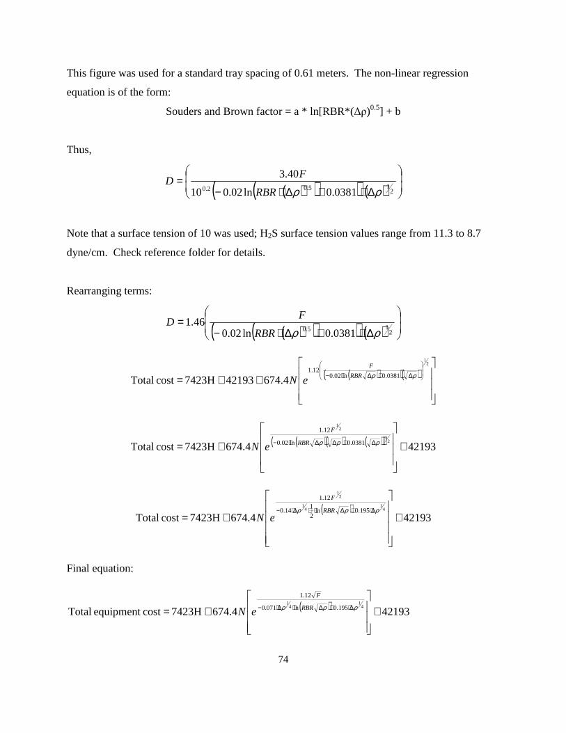
74

This figure was used for a standard tray spacing of 0.61 meters. The non-linear regression

equation is of the form:

Souders and Brown factor = a * ln[RBR*(∆ρ)0.5] + b

Thus,

( )( )( ) ( )

∆⋅+∆⋅−=

215.02.0 0381.0ln02.010

40.3

ρρRBR

FD

Note that a surface tension of 10 was used; H2S surface tension values range from 11.3 to 8.7

dyne/cm. Check reference folder for details.

Rearranging terms:

( )( )( ) ( )

∆⋅+∆⋅−=

215.0 0381.0ln02.0

46.1ρρRBR

FD

( )( )( )

++=

∆+∆⋅−

21

0381.0ln02.012.1

4.674421937423H cost Total ρρRBR

F

eN

( )( ) ( )( ) 421934.6747423H cost Total2

1

21

0381.0ln02.0

12.1

+

+= ∆+∆∆⋅− ρρρRBR

F

eN

( )421934.6747423H cost Total

41

41

21

195.0ln2

114.0

12.1

+

+=∆⋅+∆⋅⋅∆⋅− ρρρ RBR

F

eN

Final equation:

( ) 421934.6747423H cost equipment Total4

14

1195.0ln071.0

12.1

+

+= ∆⋅+∆⋅∆⋅− ρρρ RBR

F

eN

75

Derivation of Activated Sludge process: From Wikipedia.com: Atmospheric air or pure oxygen is bubbled through primary treated sewage (or

industrial wastewater) combined with organisms to develop a biological floc which reduces the organic

content of the sewage. Thus, we’re measuring outlet organic content.

What’s going on inside of an activated sludge system is the wastewater flows first through an aeration

tank where oxygen is bubbled through to create turbulent conditions. Then, the wastewater is sent to a

secondary clarifier where particles settle naturally to the bottom (bacteria consume carbonaceous matter

in the aeration tank and then settle by weight in the calm conditions of the secondary clarifier). Assume

ideal CSTR for the aeration tank. Why? Perfect mixing because oxygen is being pumped through the

aeration tank at very high speeds. It’s like a stirrer stirring the mixture.

exitA

AO

r

XFV

,−= where A is organics

( ) ( )exitA

AO

r

orgCin

orgCinorgCoutF

m

yd

ydmV

m

yd

ydCost

,3

3

33

3

3

3

,

,,

765.0

70$

765.0

70$$

−

−

⋅⋅=⋅⋅=

$70/yd is the price of concrete. A former wastewater plant operator told me that concrete was widely

used to build activated sludge systems.

( )( )

exitA

OAO

exitA

AO

r

orgCin

orgCinorgCoutvC

r

orgCin

orgCinorgCoutF

m

yd

ydCost

,,3

3

3

,

,,5.91

,

,,

765.0

70$$

−

−⋅⋅=

−

−

⋅⋅=

Using the Monod equation for biological reactions:

SM

CSA CK

CkCr

+=−

where k is the maximum utilization rate for the substrate per unit mass of bacteria

KM is the half velocity coefficient for the substrate

CS is the Cin, organics

CC = 0.1(CS0-CS)+0.001

Look on page 75 of the Kinetics reaction book for reference.

76

Thus,

( ) ( )( )( )[ ]

( )

( )[ ]orgCoutK

orgCoutorgCinorgCoutk

orgCinorgCout

m

kgton

kg

hr

tonF

orgCoutK

orgCoutorgCinorgCoutkorgCinorgCoutv

Cost

MM

O

,

001.0,,1.0,

,,1

907

5.91

,

001.0,,1.0,,,5.91

$3

++−⋅⋅

−

⋅

⋅

=

++−⋅⋅

−⋅=

because volumetric flowrate is flowrate divided by density.

I found a paper online that gave a “k” and “KM” value for phenol. Phenol is an organic. Source is down

below. k = 0.19/hr, KM = 48 ppm (mg/L).

From the book: Design and Operation of Activated Sludge Processes Using Respirometry by Alan F.

Rozich, Anthony F. Gaudy; CRC Press, 1992, page 46.

77

Finally:

( )( ) ( )

( )[ ]g

mgorgCoutorgCinorgCout

orgCoutorgCinorgCouthr

mF

Cost1000

001.0,,1.0,19.0

,48,,9075.91

$

3

⋅+−⋅⋅

+⋅−

⋅⋅

=

( ) ( ) ( )( )[ ]001.0,,1.0,

,48,,81.436$

+−⋅+⋅−⋅⋅=

orgCoutorgCinorgCout

orgCoutorgCinorgCoutFCost

where F is in ton/hr and Cout, org and Cin, org are in ppm.

That was the cost of the first part of the biological treatment (the aeration tank). There is a second part:

the secondary clarifier. Particles settle naturally (by gravity). Conditions are calm and no reaction is

occurring so neither a CSTR or a batch reactor can be used.

Reactor tank is emptied once a day. Source: wastewater plant operator. Assume 24 hr time period.

( )kg

mhr

ton

kg

hr

tonF

orgCout

orgCin

kg

mhr

ton

kg

hr

tonFEfficiencymneededVolume

333 24

907

,

,24

907 ⋅⋅⋅

⋅=⋅⋅⋅

⋅=

But, Cinorg = Coutorg, aeration tank. Cout,max = 230 ppm from the slide show (I have a reference).

Let’s specify a maximum outlet concentration to give a maximum amount of volume that we need.

We’ll use concrete as a tank material.

( ) ( )kg

mhr

ton

kg

hr

tonF

ppm

orgCin

m

yd

ydmV

m

yd

ydCost

3

3

3

33

3

3

324

907

230

,

765.0

70$

765.0

70$$ ⋅⋅⋅

⋅⋅⋅=⋅⋅=

Even though there is a recycle that enters into the clarifier, we’ll assume it is zero for now.

Finally,

( )kg

mhr

ton

kg

hr

tonF

ppm

orgCin

m

yd

ydCost

3

3

3

324

907

230

,

765.0

70$$ ⋅⋅⋅

⋅⋅⋅=

78

( )

⋅⋅=hr

tonForgCinCost ,19.8660$

( )

⋅=

hr

tonF

CostorgCin

19.8660

$,

( ) ( ) ( )( )[ ]

⋅⋅++−⋅

+⋅−⋅⋅=+=hr

tonFClarifierorgCin

AeraorgCoutorgCinAeraorgCout

AeraorgCoutorgCinAeraorgCoutFCostCostCostTotal ,,19.8660

001.0,,,1.0,,

,,48,,,81.43621$

Assume Cout,org, Aera = Cin,org, Clar = 100 ppm.

( ) ( ) ( )( )[ ]

⋅⋅++−⋅

+⋅−⋅⋅=+=hr

tonF

orgCin

orgCinFCostCostCostTotal 10019.8660

001.0100,1.0100

10048,10081.43621$

Finally,

( ) ( ) ( )( )[ ] F

orgCin

orgCinFmVCostTotal ⋅+

+−⋅−⋅⋅=⋅= 019,866

001.0100,1.0

,10048.646183$ 3

To find constraint for volume needed for the activated sludge, it is clear that any volume predicted by the

equation given below is the minimum volume needed for removing specified contaminant level. Any

volume larger is acceptable and is capable of removing more organics:

exitA

AO

r

XFV

,tankaeration −

≥ where A is organics

ForgCinkg

mhr

ton

kg

hr

tonF

ppm

orgCinV ⋅⋅≥⋅⋅⋅

⋅≥ ,64.9424907

230

, 3

clarifiersecondary

Of course, the volume needed is the addition of Vaeration tank + Vsecondary clarifier.

ForgCinr

XFVVvolumeTotal

exitA

AO ⋅⋅+−

≥+= ,64.94,

clarifiersecondarytankaeration

( ) ( )

( )[ ]ForgCin

g

mgorgCoutorgCinorgCout

orgCoutorgCinorgCouthr

mF

volumeTotal ⋅⋅+⋅+−⋅⋅

+⋅−

⋅

≥ ,64.941000

001.0,,1.0,19.0

,48,,9073

79

( ) ( )

( )[ ] ForgCinorgCoutorgCinorgCout

orgCoutorgCinorgCouthr

mF

volumeTotal ⋅⋅++−⋅

+⋅−

⋅

≥ ,64.94001.0,,1.0,

,48,,77.43

Assume Cout,org, Aera = Cin,org, Clar = 100 ppm.

( ) ( )

( )[ ] ForgCoutorgCin

orgCinhr

mF

volumeTotal ⋅⋅++−⋅

+⋅−

⋅

≥ 10064.94001.0,,1.0100

10048,10077.43

( )

( )[ ] ForgCoutorgCin

orgCinhr

mF

volumeTotal ⋅++−⋅

−

⋅

≥ 9464001.0,,1.0

,100065.73

Finally,

( )( ) F

orgCin

orgCinFV ⋅+

+−−⋅⋅≥ 9464

01.0100,

,10065.70

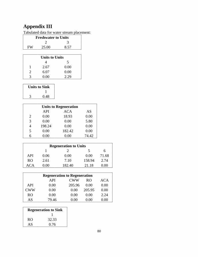
80

Appendix III Tabulated data for water stream placement:

Freshwater to Units 2 3

FW 25.00 8.57

Units to Units 4 5 1 2.67 0.00 2 6.07 0.00 3 0.00 2.29

Units to Sink 1 3 0.48

Units to Regeneration API ACA AS 2 0.00 18.93 0.00 3 0.00 0.00 5.80 4 198.24 0.00 0.00 5 0.00 182.42 0.00 6 0.00 0.00 74.42

Regeneration to Units 1 2 5 6

API 0.06 0.00 0.00 71.68 RO 2.61 7.10 158.94 2.74

ACA 0.00 182.40 21.18 0.00

Regeneration to Regeneration API CWW RO ACA

API 0.00 205.96 0.00 0.00 CWW 0.00 0.00 205.95 0.00

RO 0.00 0.00 0.00 2.24 AS 79.46 0.00 0.00 0.00

Regeneration to Sink 1

RO 32.33 AS 0.76

81

Contaminant Concentration Out of Units Salts Organics H2S Ammonia 1 101.09 500.00 286.85 67.91 2 144.40 4000.00 10.00 32.00 3 70.00 3500.00 175.00 116.67 4 66.64 502.67 20.97 46.90 5 45.48 342.84 14.17 43.47 6 2230.79 6500.00 51.38 47.93

Contaminant Concentration Into Regeneration Salts Organics H2S Ammonia

API 641.18 376.01 32.23 48.61 CWW 641.18 50.00 32.23 48.61

RO 641.18 50.00 5.00 30.00 ACA 54.40 679.69 13.68 42.26 AS 2074.55 6283.08 60.32 52.90

Contaminant Concentration Out of Regeneration Salts Organics H2S Ammonia

API 641.18 50.00 32.23 48.61 CWW 641.18 50.00 5.00 30.00

RO 20.00 50.00 5.00 30.00 ACA 54.40 75.00 13.68 42.26 AS 2074.55 60.00 60.32 52.90

82

Endnotes i Parkash, Surinder. Refining Processes Handbook. Elsevier. 2003, 254. ii Koppol, Anantha P.R., Bagajewicz, Miguel J., Dericks, Brian J., and Savelski, Mariano, J. On Zero Water Discharge Solutions in the Process Industry. Elsevier. 2002, 167. iii Gary, James H., and Handwerk, Glenn E. Petroleum Refining: Technology and Economics. 4th Ed. New York: Marcel Dekker, 2001, 2. ivhttp://www.waterandwastewater.com/www_services/ask_tom_archive/petroleum_wastewater_desalter_case_study.htm. v Gary, James H., and Handwerk, Glenn E. Petroleum Refining: Technology and Economics. 4th Ed. New York: Marcel Dekker, 2001, 47. vi Gary, James H., and Handwerk, Glenn E. Petroleum Refining: Technology and Economics. 4th Ed. New York: Marcel Dekker, 2001, 52. vii Gary, James H., and Handwerk, Glenn E. Petroleum Refining: Technology and Economics. 4th Ed. New York: Marcel Dekker, 2001, 51. viii Gary, James H., and Handwerk, Glenn E. Petroleum Refining: Technology and Economics. 4th Ed. New York: Marcel Dekker, 2001, 55. ix Kidnay, A.J., and Parrish William. Fundamentals of Natural Gas Processing. CRC Press, 2006, 228. x McKetta, John C. Petroleum Process Handbook. Marcel Dekker, Inc. 1990, 728. xi Kidnay, A.J., and Parrish William. Fundamentals of Natural Gas Processing. CRC Press, 2006, 229. xii Mohamadbigy, Kh., Bazmi, M., Behradi, R., and Binesh, R. Amine Absorption Column Design Using Mass Transfer Rate Simulation. Research Institute of Petroleum Industry. 2005, 39-46. xiii http://www.pall.com/pdf/hcp_fig_amine_sweetening.gif. xiv Gary, James H., and Handwerk, Glenn E. Petroleum Refining: Technology and Economics. 4th Ed. New York: Marcel Dekker, 2001, 176. xv http://www.emersonprocess.com/RAIhome/documents/Liq_AppData_2900-08.pdf. xvi http://www.chevron.com/products/sitelets/refiningtechnology/waste_wtr_treat_6a.aspx. xvii http://www.chevron.com/products/sitelets/refiningtechnology/waste_wtr_treat_6b.aspx. xviii http://www.wef.org/NR/rdonlyres/59E69C35-0E6F-4593-A4B8-D420AA9C4819/0/WastewaterTreatment912.pdf. xix http://engineering.dartmouth.edu/~cushman/courses/engs37/BioTreatmentTypes.pdf. xx http://www.lenntech.com/wwtp/wwtp-activated-sludge-process.htm. xxi http://www.ce.utexas.edu/prof/speitel/steady/steady.htm. xxii Seader, J.D., and Henley, Ernest J. Separation Process Principles. 2nd Ed. John Wiley & Sons, Inc. 2006, 217. xxiii http://engineering.dartmouth.edu/~cushman/courses/engs37/BioTreatmentTypes.pdf. xxiv http://www.water.siemens.com/SiteCollectionDocuments/Product_Lines/Zimpro/Brochures/ZP-APIdr-BR-0407.pdf. xxv Peters, M. S., Timmerhaus, K. D., West, R.E., Plant Design and Economics for Chemical Engineers, 5th Edition, McGraw Hill Book Co., New York, NY, 2003, 777.