water consumption levels in selected south … hub documents/research … · · 2009-09-11water...
TRANSCRIPT
WATER CONSUMPTION LEVELS IN SELECTED
SOUTH AFRICAN CITIES
Report to the Water Research Commission
by
HJ van Zyl, JE van Zyl, L Geustyn, A Ilemobade and JS Buckle
University of Johannesburg, University of the Witwatersrand
and Rand Water
WRC Report No 1536/1/06 ISBN 978-1-77005-480-6
NOVEMBER 2007

ii
DISCLAIMER
This report has been reviewed by the Water Research Commission (WRC) and approved for publication. Approval does not signify that the contents necessarily reflect the views and policies of the WRC, nor does mention of trade names or commercial products constitute
endorsement or recommendation for use.
iii
EXECUTIVE SUMMARY 1. Introduction The expansion of urban areas, the continuing development taking place in South Africa and
the constant need for potable water services have created a requirement for more accurate
water demand estimates. Inaccurate estimates lead to a deficiency in basic design information
that could lead to inadequate service provision or inequitable water distribution. In response,
this study was initiated to determine actual water demands, investigate various parameters
affecting these demands and, where possible, quantify these factors.
2. Literature review
An extensive literature review was undertaken of publications and guidelines of water
demand in South Africa. The following findings emanated from this exercise:
i. The most significant parameters that affect domestic water demand are stand area,
household income, water price, available pressure, type of development (suburban vs.
township) and climate.
ii. Some work has been done on the influence of climate. The study by Van Vuuren and Van
Beek (1997) presented interesting findings regarding the combined effect of climate and
income but was limited to the Pretoria supply area (one climatic region) and did not
consider typical low income developments. Jacobs et al. (2004) considered the influence of
climate on domestic water demand for three climatic regions but only with regards to stand
area in a single variable model. Garlipp conducted a meticulous study on the effect of
climate on domestic water demand, but considered cities as a whole (i.e. the water demand
for a city was evaluated against climate). This study investigated the effect of climate for
individual water consumers for various user categories in various types of developments
(city vs. small towns) in various climatic regions in South Africa.
iii. Most of the previous work reviewed considered parameters influencing water demand
individually. The literature review indicates that very little research has been done on non-
domestic demand patterns.

iv
iv. Most of the studies considered the Gauteng area. Only the work by Jacobs et al. (2004)
considered different geographic regions in Southern Africa and the study by Garlipp
(1979) considered other cities and regions in South Africa. However, the study by Jacobs
et al. (2004) considered a single variable namely stand area. Although Garlipp’s (1979)
work is very valuable in this regard it was undertaken nearly 30 years ago and a lot has
changed in the socio-economic and political characteristics of the country.
v. Apart from the study of Jacobs et al. (2004) that investigated nearly 600 000 domestic
users country wide, the study by Van Zyl et al. (2003) that investigated 110 000 domestic
users and the study by Husselmann (2004) with nearly 800 000 users, other studies
investigated a limited number of users.
vi. The literature review indicated that the existing design guidelines the “Red Book” (CSIR
2003) may be very conservative (Jacobs et al., 2004; Husselmann, 2004; Van Vuuren and
Van Beek, 1997).
3. Data and methodology
In recent years, GLS Consulting Engineers developed a software product called Swift. This
product allows the user to access municipal treasury databases to obtain demographic and
water consumption information for large numbers of users (domestic and non-domestic).
Swift has been implemented by many local authorities throughout South Africa, covering
different economic, socio-economic, climatic and other regions.
This study is based on water consumption data extracted from various Swift databases
developed for different municipalities throughout the country. The data reflects municipal
water meter readings used for customer billing and thus also include errors present in these
databases. Verification steps were taken to minimise the number of errors present in the
analysis.
Forty-eight municipal treasury databases were collected and extracted for archiving in this
study. This includes four metropolitan municipalities (Johannesburg, Tshwane, Ekurhuleni
and Cape Town) and 151 cities or towns. The total number of stands in the databases exceeds
2.5 million, of which 1.5 million are non-vacant stands. The number of records (i.e. water

v
meter records) in the databases exceeds 2.7 million. In most cases, the data record includes
actual water meter readings, reading dates and estimated monthly consumption figures for
more than two years. Data for all types of users with metered consumption are included in the
database, including domestic, commercial, industrial and educational users. Table 1 provides
a summary of the data according to the Department of Water Affairs and Forestry (DWAF)
Water Region and Municipality.
Table 1: Summary of Dataset Characteristics per Water Region
Water Region (DWAF) (Basson , 1997)
Municipalities Number of Data Sets
Total Number of Stands
Total Number of Vacant Stands
Total Number of Domestic Stands
Total Number of Stands with Unknown Land use
Central Sedibeng 1 170 126 129 357 144 135 8 081 Eastern Coastal Buffalo City (East London) 1 119 748 47 877 102 665 11 795
Northern Ekurhuleni, Johannesburg Water, Randfontein, Tshwane
24 1 629 636 697 706 1 377 457 155 784
South Western
BergRiver, Blaauwberg, Breede River, Breede Valley, Cape Agulhas, Cederberg, Drakenstein, Helderberg, Matzikama, Oostenberg, Overstrand, Saldanha Bay, Stellenbosch, Swartland, Theewaterskloof, Tygerberg
16 557 671 157 165 457 613 38 888
Southern Coastal
Beaufort West, George, Langeberg, Mossel Bay, Oudtshoorn, Plettenberg Bay
6 111 825 33 472 68 685 15 895
TOTAL 48 2 589 006 1 065 577 2 150 555 230 443
To ensure the integrity of the data, two data cleaning phases were implemented. In the
primary data cleaning, Swift adjustment codes (assigned where Swift identifies certain
anomalies or errors in the data) were used to exclude data that potentially contained critical
errors. In the secondary data cleaning, records flagged as vacant or not metered, pre-paid
meter records and duplicate records were excluded.
Data on climatic and socio-economic parameters that could possibly influence water
consumption was sourced from the South African Weather Service and the South African
Demarcation Board and linked to the consumption data sets.
vi
The data cleaning and verification procedure created a single database including data on water
consumption and parameters that possibly affect water demand (climate and socio-economic
data). The database was split into a number of separate databases, each database representing
a land use type, stand size and/or stand value. Filters were applied to the databases to exclude
users with unrealistically low or high stand sizes and stand values. After all data cleaning was
done, 1 091 685 records remained in the database for the analyses.
4. Domestic Water Consumption
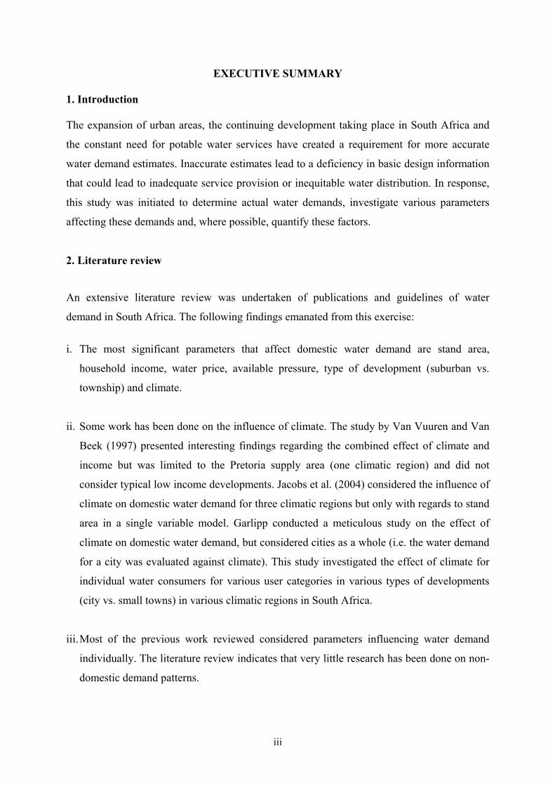
The average water consumption per suburb was calculated and compared to the current South
African design guideline as shown in Figure 1. It is clear from the figure that there is a great
deal of scatter in the demand figures, although some general trends can be discerned. It was
found that 39% of the 1 188 suburbs fell below the lower and 8% above the upper envelope
curve.
0
0.5
1
1.5
2
2.5
3
3.5
4
4.5
5
0 200 400 600 800 1000 1200 1400 1600 1800 2000
Stand Area (m2)
AA
DD
(kl/d
ay)
Red Book Lower Limit Red Book Upper Limit Data -Suburb Average
Figure 1: Average suburb consumption compared to the South African Design guidelines.

vii
Step-wise multiple variable regressions were performed on each of the domestic stand area
datasets. This determined which variables showed correlation with the water demand data and
also listed the parameters in order of significance. Single variable regressions were then done
using the most significant variable.
For example, a single variable regression analysis that was done for all 1 091 685 domestic
stands with stand size specified as the independent variable resulted in a regression equation
for the average of all stands with 95% confidence limits:
2
7 (ln 6.4124)ln( ) 1.610 0.297ln( ) 0.860 9.16 10666977
StdAreaAADD StdArea
Where StdArea is Stand Area in m2, and AADD is Annual Average Daily Demand in kl/day.
The first part of the equation (before ±) describes the average water demand curve, and the
second part the 95% confidence interval. The regression model has an adjusted R square
value of 0.218, which implies that 21.8% of the variability in the data can be explained by this
equation. An adjusted R square value of more than 20% is considered good when predicting
human behaviour as is the case with this study. The 95% confidence envelope is very small
showing a very reliable estimate for the average demand.
The main findings on domestic water demand were that inland stands use significantly more
water than coastal stands (Figure 2), and that water demand is positively correlated with both
stand value or income (Figure 3) and stand size (Figure 4). It was also concluded that the
current design guidelines underestimate the demand for small stands, and overestimate the
demand for large stands.

viii
0
0.5
1
1.5
2
2.5
3
3.5
4
0 500 1000 1500 2000 2500 3000 3500 4000
Stand Area (m 2)
AA
DD
(kl/d
ay)
Inland: Ln(AADD) = 0.314ln(StandArea) - 1.691Adjusted R2 = 0.223
Coastal: Ln(AADD) = 0.204ln(StandArea) - 1.124Adjusted R2 = 0.148
Design Guideline Upper Limit
Design Guideline Low er Limit
Figure 2: Inland and Coastal AADD as a function of stand size.
0
1
2
3
4
5
6
7
0
500
1,00
0
1,50
0
2,00
0
2,50
0
3,00
0
3,50
0
4,00
0
Stand Area (m2)
AA
DD
(kl/d
ay)
"Red Book" Upper Limit(CSIR, 2003)
"Red Book" Low er Limit(CSIR,2003)
>=R50,000 and < R100,000LOW INCOME
>=R100,000 and < R250,000LOW MIDDLE INCOME
>=R250,000 and < R500,000HIGH MIDDLE INCOME
>=R500,000 and < R750,000HIGH INCOME
`
Figure 3: AADD for different stand value (income) categories as a function of stand size.
ix
0
0.5
1
1.5
2
2.5
3
3.5
4
4.5
5
5.5
6
0
200,
000
400,
000
600,
000
800,
000
1,00
0,00
0
1,20
0,00
0
1,40
0,00
0
1,60
0,00
0
1,80
0,00
0
2,00
0,00
0
2,20
0,00
0
2,40
0,00
0
2,60
0,00
0
2,80
0,00
0
3,00
0,00
0
3,20
0,00
0
3,40
0,00
0
3,60
0,00
0
3,80
0,00
0
4,00
0,00
0
Stand Value (R)
AA
DD
(kl/d
ay)
>=500m2 and < 750m2
>=750m2 and < 1000m2
>=1000m2 and < 1500m2
>=1500m2 and < 2000m2
>=2000m2 and < 2500m2
>=2500m2 and < 3000m2
>=3000m2 and < 4000m2
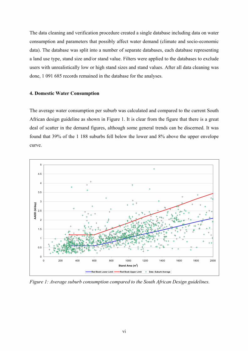
Figure 4: AADD for different stand size categories as a function of stand value
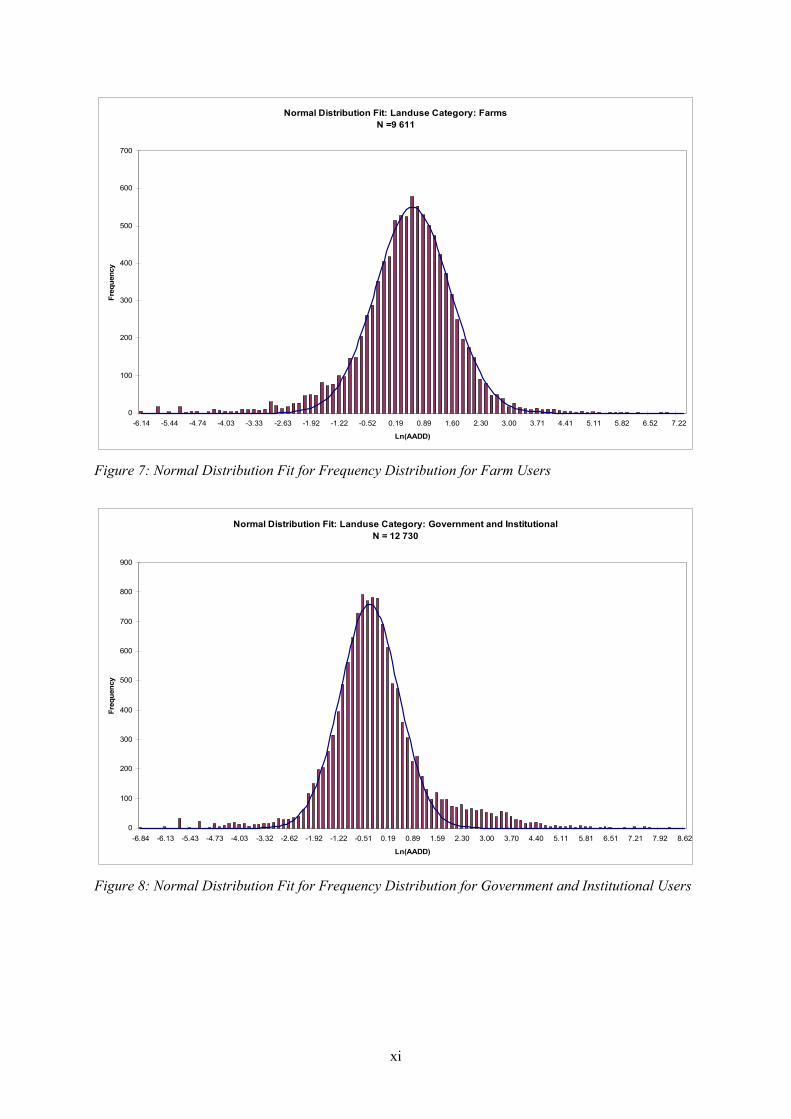
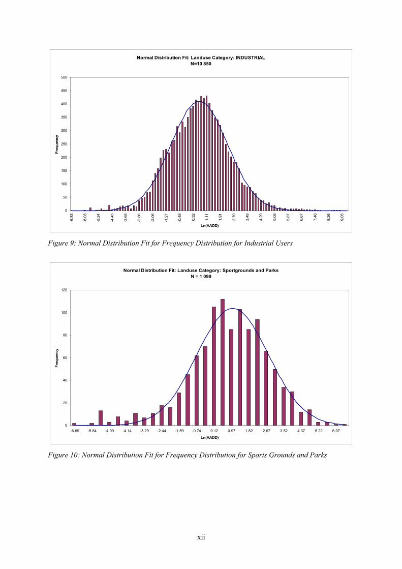
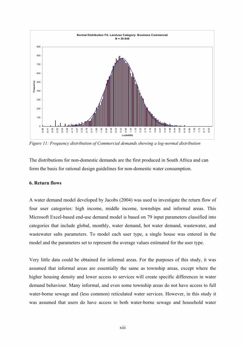
5. Non-domestic demand
Non-domestic users were grouped into seven categories: Business Commercial, Education,
Farms, Government and Institutional, Industrial, Parks and Sports. The step-wise multiple
variable regressions showed stand size and stand value to be the most significant variables for
non-domestic consumption. Good descriptions of all the non-domestic demand categories
could be made using log-normal probability distributions, as shown in Figures 5 to 11

x
Normal Distribution Fit: Landuse Category: Business CommercialN = 30 849
0
100
200
300
400
500
600
700
800
900
-6.8
6
-6.4
1
-5.9
5
-5.5
0
-5.0
4
-4.5
8
-4.1
3
-3.6
7
-3.2
2
-2.7
6
-2.3
1
-1.8
5
-1.4
0
-0.9
4
-0.4
8
-0.0
3
0.43
0.88
1.34
1.79
2.25
2.70
3.16
3.62
4.07
4.53
4.98
5.44
5.89
6.35
6.80
7.26
7.72
8.17
8.63
Ln(AADD)
Freq
uenc
y
Figure 5: Normal Distribution Fit for Frequency Distribution for Business Commercial Users
Normal Distribution Fit: Landuse Category: EDUCATIONN = 2 145
0
20
40
60
80
100
120
140
-5.67 -4.31 -2.94 -1.58 -0.21 1.15 2.51 3.88 5.24
Ln (AADD)
Freq
uenc
y
Figure 6: Normal Distribution Fit for Frequency Distribution for Educational Users
xi
Normal Distribution Fit: Landuse Category: FarmsN =9 611
0
100
200
300
400
500
600
700
-6.14 -5.44 -4.74 -4.03 -3.33 -2.63 -1.92 -1.22 -0.52 0.19 0.89 1.60 2.30 3.00 3.71 4.41 5.11 5.82 6.52 7.22
Ln(AADD)
Freq
uenc
y
Figure 7: Normal Distribution Fit for Frequency Distribution for Farm Users
Normal Distribution Fit: Landuse Category: Government and InstitutionalN = 12 730
0
100
200
300
400
500
600
700
800
900
-6.84 -6.13 -5.43 -4.73 -4.03 -3.32 -2.62 -1.92 -1.22 -0.51 0.19 0.89 1.59 2.30 3.00 3.70 4.40 5.11 5.81 6.51 7.21 7.92 8.62
Ln(AADD)
Freq
uenc
y
Figure 8: Normal Distribution Fit for Frequency Distribution for Government and Institutional Users
xii
Normal Distribution Fit: Landuse Category: INDUSTRIALN=10 850
0
50
100
150
200
250
300
350
400
450
500-6
.83
-6.0
3
-5.2
4
-4.4
5
-3.6
5
-2.8
6
-2.0
6
-1.2
7
-0.4
8
0.32
1.11
1.91
2.70
3.49
4.29
5.08
5.87
6.67
7.46
8.26
9.05
Ln(AADD)
Freq
uenc
y
Figure 9: Normal Distribution Fit for Frequency Distribution for Industrial Users
Normal Distribution Fit: Landuse Category: Sportgrounds and ParksN = 1 099
0
20
40
60
80
100
120
-6.69 -5.84 -4.99 -4.14 -3.29 -2.44 -1.59 -0.74 0.12 0.97 1.82 2.67 3.52 4.37 5.22 6.07
Ln(AADD)
Freq
uenc
y
Figure 10: Normal Distribution Fit for Frequency Distribution for Sports Grounds and Parks
xiii
Normal Distribution Fit: Landuse Category: Business Commercial
N = 30 849
0
100
200
300
400
500
600
700
800
900
-6.8
6
-6.4
1
-5.9
5
-5.5
0
-5.0
4
-4.5
8
-4.1
3
-3.6
7
-3.2
2
-2.7
6
-2.3
1
-1.8
5
-1.4
0
-0.9
4
-0.4
8
-0.0
3
0.43
0.88
1.34
1.79
2.25
2.70
3.16
3.62
4.07
4.53
4.98
5.44
5.89
6.35
6.80
7.26
7.72
8.17
8.63
Ln(AADD)
Freq
uenc
y
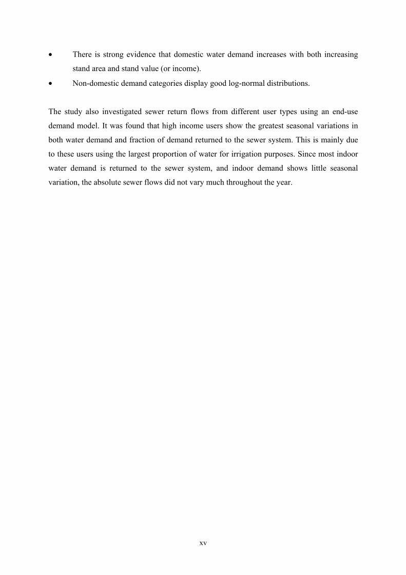
Figure 11: Frequency distribution of Commercial demands showing a log-normal distribution
The distributions for non-domestic demands are the first produced in South Africa and can
form the basis for rational design guidelines for non-domestic water consumption.
6. Return flows
A water demand model developed by Jacobs (2004) was used to investigate the return flow of
four user categories: high income, middle income, townships and informal areas. This
Microsoft Excel-based end-use demand model is based on 79 input parameters classified into
categories that include global, monthly, water demand, hot water demand, wastewater, and
wastewater salts parameters. To model each user type, a single house was entered in the
model and the parameters set to represent the average values estimated for the user type.
Very little data could be obtained for informal areas. For the purposes of this study, it was
assumed that informal areas are essentially the same as township areas, except where the
higher housing density and lower access to services will create specific differences in water
demand behaviour. Many informal, and even some township areas do not have access to full
water-borne sewage and (less common) reticulated water services. However, in this study it
was assumed that users do have access to both water-borne sewage and household water

xiv
connections, since this is the worst case scenario for sewer return flows. It also doesn’t make
sense to analyse sewer return flows in areas without water-borne sewer systems.
The results of the study showed clearly that higher income users have both higher demand
and larger variation between summer and winter demand. This is mainly due to garden
irrigation. Low income and informal settlements have very little variation in their demands.
It was also found that the return flow in the sewer system is only linked to indoor demand and
thus does not have much seasonal variation. The result is that the sewer return flow as a
percentage of the water demand shows the reverse behaviour of the water demand pattern.
The return percentage is highest for the lowest income groupings and lowest for the highest
income groupings. The highest income grouping has the greatest variation in return flow
percentage, and this percentage is highest during the winter months and lowest during the
summer months. Garden irrigation is the main reason for this behaviour.
7. Conclusions
The main part of this study consisted of an analysis of more than a million individual
consumption records, most of them longer than two years, to estimate the parameters that
influence domestic and non-domestic demands. Climatic and socio-economic census data was
also obtained and linked to the above data. Unfortunately the census data was only available
for political wards, which often include different suburbs with significantly different
properties.
Step-wise multiple variable regressions were applied to domestic and non-domestic
consumption data to determine the most significant variables in water demand. In a large
majority of cases, either the stand size or stand value had the greatest significance.
The main conclusions of the demand analyses are as follows:
47% of the average suburb demands fell inside the design envelope proposed by the
South African design guidelines.
Inland water demand is significantly higher that coastal demand.
xv
There is strong evidence that domestic water demand increases with both increasing
stand area and stand value (or income).
Non-domestic demand categories display good log-normal distributions.
The study also investigated sewer return flows from different user types using an end-use
demand model. It was found that high income users show the greatest seasonal variations in
both water demand and fraction of demand returned to the sewer system. This is mainly due
to these users using the largest proportion of water for irrigation purposes. Since most indoor
water demand is returned to the sewer system, and indoor demand shows little seasonal
variation, the absolute sewer flows did not vary much throughout the year.

xvi
ACKNOWLEDGEMENTS
The research in this report emanated from a project funded by the Water Research
Commission, entitled: “BENCHMARKING OF DOMESTIC WATER CONSUMPTION IN
SELECTED SOUTH AFRICAN CITIES” (WRC Project No K5/1525).
This project would not have been possible without financial support by the Water Research
Commission. The authors would like to extend a word of appreciation for this opportunity. Mr
JN Bhagwan, in particular, played a strong supporting and advisory role, which the authors
gratefully acknowledge.
This project was possible due to the co-operation of many individuals and institutions. The
authors therefore wish to extend their gratitude to the following:
Rand Water for the appointment to undertake the study.
Municipalities that made water consumption records available for analysis.
The South African Weather service for providing climatic data.
The South African Demarcation Board for making socio-economic statistics available.
Statistical Consulting services of the University of Johannesburg for assistance with
the statistical analyses.
GLS Consulting Engineers for providing Swift software and assistance.

xvii
TABLE OF CONTENTS EXECUTIVE SUMMARY..............................................................................................................iii ACKNOWLEDGEMENTS.............................................................................................................xvi TABLE OF CONTENTS.................................................................................................................xvii LIST OF TABLES ...........................................................................................................................xix LIST OF FIGURES .........................................................................................................................xx 1 INTRODUCTION ........................................................................................................................ 1
1.1 Background............................................................................................................................ 1 1.2 Objectives .............................................................................................................................. 2 1.3 Methodology .......................................................................................................................... 2 1.4 Layout of the Document ........................................................................................................ 5
2 LITERATURE REVIEW ............................................................................................................ 6
2.1 South African Water Demand Guidelines ............................................................................. 6 2.1.1 Domestic Water Demand................................................................................................... 6 2.1.2 Non-Domestic Water Demand .......................................................................................... 9
2.2 South African Studies of Water Demand............................................................................. 10 2.2.1 Garlipp (1979) ................................................................................................................. 10 2.2.2 Stephenson and Turner (1996)......................................................................................... 12 2.2.3 Van Vuuren and Van Beek (1997) .................................................................................. 15 2.2.4 Veck and Bill (2000) ....................................................................................................... 19 2.2.5 Van Zyl (2003) ............................................................................................................... 22 2.2.6 Jacobs (2004).................................................................................................................. 25 2.2.7 Husselmann (2004).......................................................................................................... 30
2.3 Summary of Major Unresolved Problems ........................................................................... 34 3 THE DATA ................................................................................................................................. 36
3.1 Introduction.......................................................................................................................... 36 3.2 Water Consumption Data..................................................................................................... 36
3.2.1 Data Collection ................................................................................................................ 36 3.2.2 Description of the Data.................................................................................................... 38 3.2.3 Data Verification ............................................................................................................. 43
3.3 Data on Parameters Influencing Water Consumption Patterns............................................ 48 3.3.1 Data Collection ................................................................................................................ 48 3.3.2 Description of the Data.................................................................................................... 49 3.3.3 Data Verification and Linking to Water Consumption Data ........................................... 52
4 METHODOLOGY ..................................................................................................................... 54
4.1 Data Filtering ....................................................................................................................... 54 4.2 Data Analysis and Demand Estimation ............................................................................... 58
4.2.1 Domestic Water Consumption – Assessment of the Existing Design Guidelines........... 58 4.2.2 Assessment of Factors Influencing Domestic Water Consumption ................................ 58 4.2.3 Non-Domestic Water Consumption ................................................................................ 59
5 RESULTS.................................................................................................................................... 61
5.1 Domestic Water Consumption............................................................................................. 61 5.1.1 Assessment of the Existing Design Guidelines ............................................................... 61 5.1.2 Assessment of Factors Influencing Domestic Water Consumption ................................ 66
5.2 Non-Domestic Water Consumption..................................................................................... 84 5.2.1 Frequency Distribution of Non-Domestic Water Consumption Data ............................. 84 5.2.2 Assessment of Factors Influencing Non-Domestic Water Consumption ........................ 88

xviii
6 RETURN FLOW ESTIMATION ........................................................................................... 105 6.1 Introduction........................................................................................................................ 105 6.2 End-use demand and return flow model ............................................................................ 105 6.3 Sources of information....................................................................................................... 107 6.4 Parameters.......................................................................................................................... 107
6.4.1 Household size............................................................................................................... 107 6.4.2 Bath................................................................................................................................ 108 6.4.3 Shower........................................................................................................................... 108 6.4.4 Toilet.............................................................................................................................. 109 6.4.5 Clothes washing............................................................................................................. 109 6.4.6 Dishwasher .................................................................................................................... 109 6.4.7 Other volume based demands........................................................................................ 110 6.4.8 Other time based demands............................................................................................. 110 6.4.9 Garden irrigation............................................................................................................ 110 6.4.10 Swimming pool ......................................................................................................... 111 6.4.11 On-site leakage.......................................................................................................... 111 6.4.12 Water temperatures ................................................................................................... 111 6.4.13 Parameter summary................................................................................................... 112
6.5 Model calibration ............................................................................................................... 112 6.6 Results and discussion ....................................................................................................... 113 6.7 Conclusions........................................................................................................................ 115
7 CONCLUSIONS....................................................................................................................... 116 8 REFERENCES ......................................................................................................................... 118 PLEASE NOTE THAT THE FOLLOWING APPENDICES ARE SUPPLIED ON THE ATTACHED CD, WITH A PDF VERSION OF THE FINAL REPORT : APPENDIX A: DATA CHARACTERISTICS (Supplied in electronic format only) APPENDIX B: CLIMATIC DATA (Supplied in electronic format only) APPENDIX C: REGRESSION RESULTS (Supplied in electronic format only)

xix
LIST OF TABLES Table 2-1: Domestic Water Demand for Developing Areas (CSIR, 2003 – Table 9.10)........................ 7 Table 2-2: Domestic Water Demand in Developing Areas Equipped with Standpipes, Yard
Connections and House Connections (CSIR, 2003 – Table 9.11)................................................. 7 Table 2-3: Non-Domestic Water Demand in Developing Areas (CSIR, 2003 – Table 9.12) ................. 9 Table 2-4: Non-Domestic Water Demand in Developed Areas (CSIR, 2003 – Extract of Table 9.14).. 9 Table 2-5: Water Price Elasticity (Veck and Bill, 2000)....................................................................... 20 Table 2-6: Perceived Water Usage for Various Income Groups (Veck and Bill, 2000) ....................... 21 Table 2-7: Effect of Water Price on Domestic Demand (Van Zyl , 2003)............................................ 24 Table 2-8: Stand Area and Stand Value Categories used in the study by Husselmann (2004) ............. 31 Table 3-1: Summary of Municipal Treasury Data Used. ...................................................................... 38 Table 3-2: Summary of Dataset Characteristics per Water Region....................................................... 41 Table 3-3: Primary Data Cleaning Procedure ....................................................................................... 44 Table 3-4: Standardised Land Use Codes Used .................................................................................... 46 Table 3-5: Data Sources for Parameters Influencing Water Demand ................................................... 49 Table 3-6: Climatic Data Supplied by the SAWS ................................................................................. 50 Table 4-1: Data Filters Applied to Water Consumption Data ............................................................... 55 Table 4-2: Final Sizes of the Domestic Datasets for Categories of Stand Value .................................. 56 Table 4-3: Final Sizes of the Domestic Datasets for Categories of Stand Area .................................... 57 Table 4-4: Final Sizes of the Non-Domestic Datasets........................................................................... 57 Table 5-1: Summary of the Outcome of the Stepwise Multi-Variable Regression Analyses on
Domestic Categories.................................................................................................................... 66 Table 5-2: Definition of Income Level Used in the Study .................................................................... 71 Table 5-3: Regression Results (First Step) of the Stepwise Multiple Variable Regression Analyses for
Categories of Stand Area ............................................................................................................. 72 Table 5-4: Regression Results (First Step) of the Stepwise Multiple Variable Regression Analyses for
Categories of Stand Value............................................................................................................ 72 Table 5-5: Single Variable Regression Results for Domestic Categories ............................................. 75 Table 5-6: Summary of the Outcome of the Stepwise Multiple Variable Regression Analysis of Non-
Domestic Users Categories .......................................................................................................... 88 Table 5-7: Single Variable Regression Results for Non-Domestic User Categories with Distinction
Made for Development Level and Geographic Location............................................................. 92 Table 5-8: Summary of the Single Variable Regression Analyses for Non-Domestic Users Categories
.................................................................................................................................................... 103 Table 6-1: Significance index for output parameters (Jacobs, 2004) .................................................. 106 Table 6-2: Summary of parameters used............................................................................................. 112

xx
LIST OF FIGURES
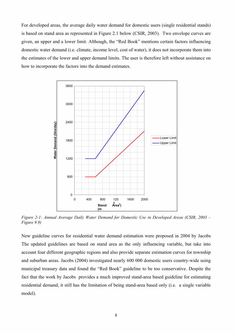
Figure 2-1: Annual Average Daily Water Demand for Domestic Use in Developed Areas (CSIR, 2003 – Figure 9.9)................................................................................................................................... 8
Figure 2-2: Evaluation of Existing Guidelines for Domestic Water Demand in the Gauteng Area (Stephenson and Turner, 1996) .................................................................................................... 13
Figure 2-3: Effect of Income – (Stephenson and Turner, 1996) ........................................................... 14 Figure 2-4: Evaluation of Existing Guidelines for Domestic Water Demand for the Pretoria Supply
Area (Van Vuuren and Van Beek, 1997) ..................................................................................... 18 Figure 2-5: Effect of an Increase in Water Price on Water Demand (Veck and Bill, 2000) ................. 21 Figure 2-6: Southern African Coastal Winter Rainfall Region Model (Suburban and Townships)
(Jacobs , 2004) ............................................................................................................................. 27 Figure 2-7: Southern Africa Inland Summer Rainfall Region Model- Suburban (Jacobs , 2004) ........ 28 Figure 2-8: Southern Africa Inland Summer Rainfall Region Model – Townships (Jacobs , 2004) .... 28 Figure 2-9: Southern Africa Coastal Annual Rainfall Region Model (Suburban & Townships)
Restricted to George (Jacobs , 2004) ........................................................................................... 29 Figure 2-10: AADD vs. Stand Area for the R 65 000 to R85 000 Stand Value Category.” Red Book”
(CSIR,2003) is also shown. (Husselmann, 2004) ........................................................................ 31 Figure 2-11: AADD as a Function of Stand Area for Different Stand Value Categories (Husselmann,
2004) ............................................................................................................................................ 32 Figure 2-12: Proposed New Design Envelope for AADD showing data points and the Red Book
Envelopes (Husselmann, 2004).................................................................................................... 33 Figure 3-1: Geographic Locations of the Municipalities Studied ......................................................... 40 Figure 3-2: Monitoring Period of Each Dataset Used in the Study....................................................... 42 Figure 4-1: Single Variable Regression Models for Domestic User Categories ................................... 59 Figure 4-2: Single Variable Regression Models for Non-Domestic User Categories........................... 60 Figure 5-1: Preliminary Assessment of the Existing Demand Estimation Guidelines.......................... 61 Figure 5-2: Single Variable Regression Model with Stand Area for All Domestic Data...................... 63 Figure 5-3: Confidence Intervals for the Single Variable Regression Model for Domestic Use (all data
points)........................................................................................................................................... 64 Figure 5-4: Single Variable Regression Models for the Inland and Coastal Categories ....................... 65 Figure 5-5: Regression Results (First Step) of the Stepwise Multiple Variable Regression for Stand
Area Categories............................................................................................................................ 73 Figure 5-6: Regression Results (First Step) of the Stepwise Multiple Variable Regression for Stand
Value Categories .......................................................................................................................... 74 Figure 5-7: Single Variable Regression Analysis (AADD vs. Stand Area) for Categories of Stand
Value (Income) and Geographic Location is Inland .................................................................... 81 Figure 5-8: Single Variable Regression Analysis (AADD vs. Stand Area) for Categories of Stand
Value (Income) and Geographic Location is Coastal .................................................................. 82 Figure 5-9:Single Variable Regression Analysis (AADD vs. Stand Value) for Categories of Stand
Value (Income) and Geographic Location is Inland .................................................................... 83 Figure 5-10: Single Variable Regression Analysis (AADD vs. Stand Value) for Categories of Stand
Value (Income) and Geographic Location is Coastal .................................................................. 84 Figure 5-11: Normal Distribution Fit for Frequency Distribution for Business Commercial Users..... 85 Figure 5-12: Normal Distribution Fit for Frequency Distribution for Educational Users..................... 85 Figure 5-13: Normal Distribution Fit for Frequency Distribution for Farm Users ............................... 86 Figure 5-14: Normal Distribution Fit for Frequency Distribution for Government and Institutional
Users............................................................................................................................................. 86 Figure 5-15: Normal Distribution Fit for Frequency Distribution for Industrial Users ........................ 87 Figure 5-16: Normal Distribution Fit for Frequency Distribution for Sportgrounds and Parks............ 87 Figure 5-17: Comparison of the First Step of the Stepwise Multiple Variable Regression Models for
Industrial, Education, Government and Parks User Categories ................................................... 90 Figure 5-18: Comparison of the First Step of the Stepwise Multiple Variable Regression Analysis for
Business Commercial and Farms User Categories ...................................................................... 91
xxi
Figure 5-19: Single Variable Regression Results: AADD vs. Stand Value for Business Commercial Users............................................................................................................................................. 96
Figure 5-20: Single Variable Regression Results: AADD vs. Stand Area for Business Commercial Users............................................................................................................................................. 97
Figure 5-21: Single Variable Regression Results: AADD vs. Stand Value for Educational Users ...... 97 Figure 5-22: Single Variable Regression Results: AADD vs. Stand Area for Educational Users ........ 98 Figure 5-23: Single Variable Regression Results: AADD vs. Stand Value for Farm Users................. 98 Figure 5-24: Single Variable Regression Results: AADD vs. Stand Area for Farm Users................... 99 Figure 5-25: Single Variable Regression Results: AADD vs. Stand Value for Government and
Institutional Users ........................................................................................................................ 99 Figure 5-26: Single Variable Regression Results: AADD vs. Stand Area for Government and
Institutional Users ...................................................................................................................... 100 Figure 5-27: Single Variable Regression Results: AADD vs. Stand Value for Industrial Users ........ 100 Figure 5-28: Single Variable Regression Results: AADD vs. Stand Area for Industrial Users.......... 101 Figure 5-29: Single Variable Regression Results: AADD vs. Stand Value for Parks Users .............. 101 Figure 5-30: Single Variable Regression Results: AADD vs. Stand Area for Parks Users ................ 102 Figure 5-31: Single Variable Regression Results: AADD vs. Stand Area for Sports Users............... 102 Figure 6-1: Calculated water demand patterns.................................................................................... 113 Figure 6-2: Calculated sewer return flow patterns .............................................................................. 114 Figure 6-3: Fraction of water demand returned to the sewer system .................................................. 114

xxii

1
1 INTRODUCTION 1.1 Background
The underlying motive of this study was the conservation of a limited natural resource that is
indispensable for human life. Proper planning and future water demand management is essential in
an economically developing and water scarce country such as South Africa.
A key input in water demand management and planning for municipal services is the estimation of
present and prediction of future water demand. Water demand estimates are used to calculate peak
water demand and sewer flows and thus determines municipal water and sewer infrastructure
requirements, which in turn decide water authorities’ budgets and capital investment needs.
The literature review that was undertaken as part of this study indicated that annual average water
consumption is a function of a large number of variables, including type of supply, land use, climate,
stand size, population density, and the socio-economic profile of the supply area. The document
“Guidelines for Human Settlement Planning and Design” (CSIR 2003) is commonly used in South
Africa to estimate municipal water demand. In this guideline, water demand is linked to the type of
supply and whether the supply area is a developing or developed community. The guideline provides
upper and lower limits for annual average demand in residential stands based on stand size. The
designer has to take other factors, such as climate and income into account when selecting an
appropriate demand for a given area.
The expansion of urban areas, the continuing development taking place in South Africa and the
constant need for potable water services have created a requirement for more accurate water demand
estimates. Inaccurate estimates lead to a deficiency in basic design information that could lead to
inadequate service or inequitable water distribution. In response to this need the Water Research
Commission (WRC) has sponsored this study in South Africa to determine actual water demands, and
investigate various parameters possibly affecting these demands and, where possible, quantify these
factors. In 2004, the WRC awarded the current research contract to Rand Water. Due to a reduction in
the funding available for the project, Rand Water in turn contracted the Water Research Group of the
University of Johannesburg in 2005 to conduct the research.

2
1.2 Objectives
The following aims were set for the project:
To determine the water consumption per stand for selected South African towns/cities.
To relate the water consumption per stand to the stand size, the stand value and other
influencing factors.
To determine the seasonal variation in water demand
To estimate the return flow per stand for selected South African towns/cities.
To relate the return flow per stand to the various influencing factors.
To estimate the seasonal variation in return flow
The data obtained has greatly exceeded the original estimate of a few hundred thousand records.
The total data set collected for the analysis is shown in Table 3.1. It comprises of 2 792 053
records from 151 cities and towns throughout the country. In most cases, the data for each record
include the monthly water consumption figures for at least two years. Furthermore, a thorough
analysis of non-domestic demands was done, which was not part of the original proposal.
As a result of the enormous data set, it was proposed that the focus of the study is shifted towards
analysing average water demand rather than seasonal variations and sewer return flows. Thus, the
sewer return flow evaluation only comprised of a desk top analysis and no field verification of
return flows was done.
1.3 Methodology
The main difference in the methodology of this study and those of many previous studies is that in
this study municipal water meter readings were used to determine water demand information. This
made it possible to study a very large number of consumers. This is much more than could ever be
hoped to be evaluated with a logging exercise. A large number of records made it possible to
conduct meticulous statistical analyses, to investigate the distribution of the data in greater detail
and to have representative samples of specific data characteristics.
The overriding problem with studying water demand is that quality data is not readily available.
Even a large logging exercise can realistically only reach a small proportion of users. Furthermore,
3
a logging survey is expensive and therefore further limits the length of the monitoring period and
the number of users monitored. This study considered municipal water meter readings to be an
ideal source of water demand information, since the readings are taken on a regular basis by
virtually all municipalities in South Africa. Possible arguments against using meter readings for
studying water demand are:
Consumer meters do not accurately register the amount of water used.
It is difficult to access and extract water demand information from municipal treasury
systems.
Meter readings are not always taken monthly and are estimated for some months.
Meter readings are not always accurate as meters clock over or meter replacements take
place.
Customer information such as address, income level or user type contained in treasury
systems is not always accurate.
It is true that the accuracy of a consumer meter declines over the years. However, it is in the
interest of the utility (municipality) and the consumer that the meter register as accurately as
possible the amount of water used and therefore meter maintenance programmers should be in
place in most utilities. Meters seldom are designed to under-register as they age in order to benefit
the customer rather that the water utility (Garlipp, 1979). It was assumed for this study that the
accuracy of the consumer meters studied is adequate.
Until recently, the wealth of water demand information in municipal treasury systems was difficult
to access. Actual meter readings were often hidden in complicated database setups or could not be
directly or easily linked to user information. In most cases it was not possible to analyse data
programmatically i.e. using a computer and software. However, the past decade has seen
significant software developments that now enable engineers to abstract and analyse demand
information from treasury databases for selected municipalities that have employed these software
tools (Jacobs et al., 2004). One such software tool is Swift. This software allows a user to
interrogate and access municipal treasury databases to obtain demographic data, stand
characteristics (size and value) and recorded water consumption for individual consumer
connections. A number of municipalities have implemented Swift including Tshwane
Metropolitan Municipality, Ekurhuleni, Johannesburg Water and most of the municipalities of the
Western Cape. The existing databases cover years of consumption data for hundreds of thousands
of users. This study therefore, with the collaboration of GLS Consulting Engineers and the various

4
municipalities, extracted recorded monthly meter readings with the associated demographic and
stand characteristics for more than 2.5 million stands for at least a period of 2 years from 48
different municipalities countrywide.
To address problems like meter clock overs or replacements, this study made use of the data
cleaning functions contained in Swift In addition to the Swift data cleaning procedures this study
also followed a rigorous data cleaning process to ensure the integrity of the final data used for
analysis. Even given the thorough data cleaning and filtering procedures that were applied, it is
expected that some inaccurate data will still be contained in the dataset. This is one of the
limitations of this study. However, a very large number of records (more than a million) was
analysed and therefore although data inaccuracy will inevitably lead to some degree of variation in
the final results, significant correlations and trends are still expected.
Municipalities used in the study were selected based on their economic importance and distribution
to represent different climatic and economic regions of South Africa in the study and of course on
the availability of the data. It was decided to undertake the water demand part of the study in five
main tasks:
Task 1: Identify and confirm the towns and cities in terms of the available data and
willingness to be involved in study. Collect the available data
Task 2: Extract the relevant data from the available treasury databases. Verify and clean the
data. Obtain specific characteristics of each dataset in order to confirm that a representative
sample of users will be studied with regards to economic, climatic and user type
characteristics.
Task 3: Data analyses to determine relationships between the average daily demand and
stand size, stand value, household income level, household size, season, and other potential
parameters.
Task 4: Evaluation of the current South African guidelines commonly used to estimate
domestic and non-domestic water demand, given the outcome of the study analyses
Task 5: Documentation of the results.
The study has a number of limitations, including the following:
Water consumption is an inherently variable process and any measured data will thus include a
measure of variability and uncertainty.
5
Alternative water sources were not considered in this study. The treasury data does not identify
stands with alternative water sources. The most common alternative sources are groundwater from
boreholes, rainwater collected from roofs and on-site re-use of grey water. Usually water from
alternative sources in residential developments is used for garden irrigation. This will definitely
influence water demand patterns in the affected stands (most likely larger residential stands). The
study intends to investigate demand patterns of non-domestic water demand. However, it is
understood, that this analysis will rely greatly on the accuracy of the user type codes assigned to
the non-domestic users in the treasury data.
The climatic parameters that were included relate to the measurement years of the treasury data for
the specific datasets. The weather parameters during the time of demand measurement were not
compared to the long term average to check whether the measured water demand was subjected to
significant influences by abnormal weather patterns.
1.4 Layout of the Document
The main document consists of seven chapters that consist of the following:
Chapter 1: Introduction.
Chapter 2: Literature review of existing design guidelines and previous work.
Chapter 3: Data used in this study, including data collection, cleaning and verification
processes.
Chapter 4: Data analysis methodology used to analyse the data.
Chapter 5: Results of the analyses.
Chapter 6: Conclusions.
Three appendixes form part of the report, although they are only provided in electronic format. The
appendixes consist of the following:
Appendix A: Detailed description of the characteristics of the data used in this study.
Appendix B: Climatic data that was used in the study with regards to mean annual
precipitation and mean annual evaporation measurements.
Appendix C: All the regression results obtained from the data analyses.

6
2 LITERATURE REVIEW 2.1 South African Water Demand Guidelines
2.1.1 Domestic Water Demand The estimation of peak water demands often consisted of estimating the population, multiplying by
an average daily per capita use and then applying peak-to-average ratios based on entire cities
(Howe & Linaweaver, 1967). It has been recognised that domestic water demand estimates should
be preferably based on actual water consumptions per township as recorded by the municipal
treasury (City of Johannesburg, 1989; Howe & Linaweaver, 1967). However, information on
actual water consumptions is not always readily available and as a consequence guidelines for
domestic demand estimation are still mostly based on stand area (Jacobs , 2004; CSIR, 2003)
The first guideline that was compiled in South Africa with the aim to provide information with
regards to the provision of engineering services in residential townships was the so-called “Blue
Book” (CSIR, 1983), taking its name from the ring binder in which it was issued. It was published
by the Department of Community Development and it was based on the experience of various
municipal, design and planning engineers and town planners and it had the input of several
technical committees. One of the sections of the “Blue Book” is dedicated to water supply. It
contains information regarding design criteria, materials, construction and provides guidelines for
demand estimation for water reticulation design and storage facilities. The “Blue Book” is mainly
only applicable to urban residential areas with access to water-borne sanitation.
In the late 1980’s the Department of Development Aid with support of the South African Housing
Advice Council developed a guideline for the provision of engineering services for developing
communities with a focus on low cost services, the so-called “Green Book” (1986). In 1994, the
CSIR published a revised guideline that addressed and combined the guidelines of the “Blue
Book” and the “Green Book” with the title “Guidelines for the Provision of Engineering Services
and Amenities in Residential Township Development” the so-called “Red Book” (CSIR, 1994).
The “Red Book” has been revised since its publication in 1994. The first “Red Book” was
considered to have a number of shortcomings which restricted its usefulness in the drive to
produce sustainable and vibrant human settlements as opposed to mere human settlements (CSIR,
2003). In terms of its mandate, the CSIR Division of Building and Construction Technology has
undertaken to maintain the “Red Book” as a continually updated “living document” (CSIR, 2003).
A revision of the ”Red Book” was published in 2000, with another revision in August 2003. The
revisions in August 2003 applied to Chapter 9-Water Supply and Chapter 10-Sanitation.

7
The average water demand estimation guidelines of the most recent publication of the “Red Book”
(CSIR, 2003) have remained unchanged since the first publication of the original guideline in the
“Blue Book” (CSIR, 1983). However, the most recent publication of the guideline distinguishes
between water demand in developing and developed areas. The following definitions are given
(CSIR, 2003):
“Developing areas are considered to be those areas where the level of services to be installed may
be subject to future upgrading to a higher level.”
“Developed areas are considered to be those areas where the services installed are already at
their highest level and therefore will not require future upgrading.”
Table 2.1 and Table 2.2 summarise the “Red Book” guideline for domestic water demand in
developing areas.
Table 2-1: Domestic Water Demand for Developing Areas (CSIR, 2003 – Table 9.10)
Type of Water Supply Typical Consumption (litre/ca/d)
Range (litre/ca/d)
Communal Water Point Well or standpipe at considerable
distance (>1000 m) 7 5-10
Well or standpipe at medium distance (250 - 1 000 m) 12 10-15
Well nearby (<250 m) 20 15-25
Table 2-2: Domestic Water Demand in Developing Areas Equipped with Standpipes, Yard Connections and House Connections (CSIR, 2003 – Table 9.11)
Type of Water Supply Type of Consumption (litre/ca/d)
Range (litre/ca/d)
Standpipe (200 m walking) 25 10-50 Yard Connection With dry sanitation With LOFLOs With full-flush sanitation
55
50-100 30-60 45-75 60-100
House connection (developed areas) Development level: Moderate Moderate to high High Very high
80 130 250 450
60-475
48-98 80-145
130-280 260-480
8
For developed areas, the average daily water demand for domestic users (single residential stands)
is based on stand area as represented in Figure 2.1 below (CSIR, 2003). Two envelope curves are
given, an upper and a lower limit. Although, the “Red Book” mentions certain factors influencing
domestic water demand (i.e. climate, income level, cost of water), it does not incorporate them into
the estimates of the lower and upper demand limits. The user is therefore left without assistance on
how to incorporate the factors into the demand estimates.
Figure 2-1: Annual Average Daily Water Demand for Domestic Use in Developed Areas (CSIR, 2003 – Figure 9.9)
New guideline curves for residential water demand estimation were proposed in 2004 by Jacobs
The updated guidelines are based on stand area as the only influencing variable, but take into
account four different geographic regions and also provide separate estimation curves for township
and suburban areas. Jacobs (2004) investigated nearly 600 000 domestic users country-wide using
municipal treasury data and found the “Red Book” guideline to be too conservative. Despite the
fact that the work by Jacobs provides a much improved stand-area based guideline for estimating
residential demand, it still has the limitation of being stand-area based only (i.e. a single variable
model).
0
600
1200
1800
2400
3000
3600
0 400 800 1200
1600 2000
Stand Area (m
2)
Wat
er D
eman
d (li
tre/
day)
Lower Limit Upper Limit

9
2.1.2 Non-Domestic Water Demand
It is generally recommended that non-domestic water demands should be based on field
measurements as it is extremely difficult to estimate non-domestic demand (CSIR, 2003). The City
of Johannesburg also recommends in its water supply guidelines that non-domestic demands
should be determined where possible from the City Treasurer’s records on actual water
consumption (City of Johannesburg, 1989).
The “Red Book” guideline with regards to non-domestic water demand is summarised in Tables
2.3 for developing areas and Table 2.4 for developed areas.
Table 2-3: Non-Domestic Water Demand in Developing Areas (CSIR, 2003 – Table 9.12)
Non-Domestic Users Water Demand Schools: Day Boarding
15-20 90-140 litres/pupil/day
Hospitals 220-300 litres/bed/day Clinics 5 litres/bed/day – out patients
40-60 litres /bed/day – in patients Bus stations 15 litres/user/day for those persons outside the
community Community Halls / Restaurants 65-90 litres/seat/day
Table 2-4: Non-Domestic Water Demand in Developed Areas (CSIR, 2003 – Extract of Table 9.14)
Category Type of Development Unit
Annual Average Water Demand
(litres/day) unless otherwise stated
4 Offices and Shops 100 m2 of gross floor areaa 400 5 Government and municipal 100 m2 of gross floor area 400 6 Clinic 100 m2 of gross floor area 500 7 Church Erf 2000 8 Hostels Occupant 150
9 Developed Parks Hectare of erf area
=<2 ha: 15 klb,c
>2 ha and =<10 ha : 12.5 kl >10 ha: 10 kl
10 Day School / Crèche Hectare of erf area As per developed parksd
11 Boarding School Hectare of erf area plus boarders
As per developed parks plus 150 litre/boarder
12 Sports ground Hectare of erf area As per developed parks
a: Gross floor area obtained using applicable floor space ratio from town planning scheme
b: Demand for developed parks to be considered as drawn over six hours on any particular day in order to obtain the peak demand
c: Where the designer anticipates the development of parks and sports grounds to be of a high standard, e.g. 25 mm of water
applied per week, the annual average water demand should be taken as follows: =<2 ha: 50 klitre; >2 ha and =<10 ha: 40 klitre ;
>10 ha : 30 klitre
10
2.2 South African Studies of Water Demand
The following sections provide a summary of the literature review specifically with regards to
previous work done in South Africa in the field of municipal water demand estimation. The
highlights and limitations of the previous studies are summarised to bring to light the remaining
unresolved problems that this study intended to address.
2.2.1 Garlipp (1979)
The research conducted by Garlipp studied domestic demand in various South African cities and
also the possible factors influencing domestic demand. Water consumption was studied for cities
as a whole (Pretoria, Bloemfontein, Cape Town, Port Elizabeth and Durban) and for individual
consumers and sectors. Data was sourced from meter readings and water meter books (individual
customers). Sample sizes were approximately 20% of the residential sectors of the cities studied.
The study provides a breakdown of internal and external domestic water consumption in three
South African cities namely Durban, Johannesburg (Witwatersrand) and Cape Town (Cape
Peninsula). The data for this analysis was obtained by sending out questionnaires to the
engineering population of South Africa. The author found that 73% of domestic consumption in
the Witwatersrand was for outdoor use compared to the Cape Peninsula where only 40% of
domestic water consumed was used outdoors. In Durban, 45% of domestic water consumed was
used outdoors. Garlipp also found that the average daily domestic consumption in the
Witwatersrand (2240 litres/stand/day) was significantly more than in the Cape Peninsula (914
litres/stand/day).
Garlipp also studied climatic variables and related water consumption patterns. This was
investigated for entire cities (i.e. base unit is a city). It was found that after prolonged rainfall,
water consumption decreased. Temperature had a positive correlation with water consumption i.e.
with an increase in temperature, water consumption increased. An interesting finding is that
domestic water was largely consumed internally at lower temperatures and externally at higher
temperatures. This study evaluated seasonal variation in water demand for entire cities (i.e. base
unit is a city) in Southern Africa and found that at least one month each year was found to have a
monthly consumption that was less than 80% of the average annual monthly consumption. The
author mentioned a study on Southern African cities that indicated that water consumption could
be the result of differential tariff structures, restriction of water flows or restricting consumption

11
for certain purposes such as garden watering in drought periods. The author pointed out that
differential water tariffs in Windhoek saved approximately 20% water over a 6 month period.
Garlipp stated that metering in conjunction with regular reading and an effective tariff structure
and diligent collection system could reduce water consumption significantly.
Garlipp found the most significant parameter that influences domestic water consumption to be
household size. This South African study indicated that water consumption per capita increased
with stand area and income but decreased with an increase in household size. Household size did
not affect external domestic water use. This study found that income influenced domestic water
consumption positively and followed an S- curve. Stand area was also found to have a positive
correlation with domestic water use. It significantly influenced external domestic use. The type of
stand coverage (i.e. grass, paving, shrubbery etc.) was one of the main factors determining external
domestic use. Garlipp also considered stand area as a good proxy for income. Boreholes were also
found to significantly affect external domestic use. It was found that less water was consumed
externally on stands with access to boreholes.
Highlights and Limitations of the Study
i. The study by Garlipp is the first of its kind in South Africa and was conducted before the
publication of the “Blue Book”. It provided a valuable base for further research in water
demand estimation in South Africa.
ii. The study investigated the effect of a number of factors on domestic water demand patterns
in urban areas countrywide in five different cities. The study found household size was the
most significant parameter that influenced domestic water demand. Other factors that
positively affected domestic demand were income, stand area (only external use) and
prolonged high temperatures. Access to borehole water and rainfall had a negative
correlation with domestic water demand.
iii. The study measured water demand for cities as a whole and thus evaluated the effect of
climatic factors on the basis of an entire city. Socio-economic data such as income, stand
area and household size were collected by means of surveys. The response on these surveys
was poor and various questionnaires had to be sent out. Some of the surveys were only
conducted among the engineering fraternity of South Africa, which may be viewed as a
biased sample.
iv. The study distinguished between ethnicity in most of its results, the research being
conducted in a previous political era. This makes it difficult to compare with research being
conducted in current day South Africa.
12
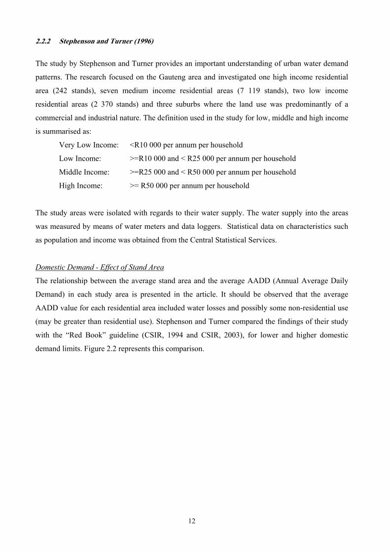
2.2.2 Stephenson and Turner (1996)
The study by Stephenson and Turner provides an important understanding of urban water demand
patterns. The research focused on the Gauteng area and investigated one high income residential
area (242 stands), seven medium income residential areas (7 119 stands), two low income
residential areas (2 370 stands) and three suburbs where the land use was predominantly of a
commercial and industrial nature. The definition used in the study for low, middle and high income
is summarised as:
Very Low Income: <R10 000 per annum per household
Low Income: >=R10 000 and < R25 000 per annum per household
Middle Income: >=R25 000 and < R50 000 per annum per household
High Income: >= R50 000 per annum per household
The study areas were isolated with regards to their water supply. The water supply into the areas
was measured by means of water meters and data loggers. Statistical data on characteristics such
as population and income was obtained from the Central Statistical Services.
Domestic Demand - Effect of Stand Area
The relationship between the average stand area and the average AADD (Annual Average Daily
Demand) in each study area is presented in the article. It should be observed that the average
AADD value for each residential area included water losses and possibly some non-residential use
(may be greater than residential use). Stephenson and Turner compared the findings of their study
with the “Red Book” guideline (CSIR, 1994 and CSIR, 2003), for lower and higher domestic
demand limits. Figure 2.2 represents this comparison.

13
0
600
1200
1800
2400
3000
3600
0 400 800 1200 1600 2000
Stand Area (m2)
Wat
er D
eman
d (li
tre/d
ay/s
tand
)
Red Book Lower Limit (CSIR, 1994)
Red Book Upper Limit (CSIR, 1994)
Stephenson & Turner
L - Alexandra
L- Rabie Ridge
MM
M
M
M
MM
H
L = low incomeM = middle incomeH = high income
Figure 2-2: Evaluation of Existing Guidelines for Domestic Water Demand in the Gauteng Area (Stephenson and Turner, 1996)
Figure 2.2 indicates that the average per stand water demand of the majority of the study areas fell
within the design guideline envelope recommended by the “Red Book” (CSIR, 1994 and 2003).
The areas whose average per stand consumptions did not fall within the guideline envelope were
low income areas. The one area, Alexandra, had domestic water demand much higher than
predicted by the guideline. Stephenson and Turner noted that the study area in Alexandra was
unusually densely populated which resulted in very high demand per stand. The other low income
area investigated by Stephenson and Turner, i.e. Rabie Ridge had significantly lower water
demand than anticipated by the lower limit of the guideline curve (CSIR, 1994 and 2003).
Stephenson and Turner indicated that the reason might be that Rabie Ridge had no house
connections or waterborne sanitation (at the time of the study.)
This study concluded that generally it could be said that stand area had a direct influence on water
demand. However, the type of housing had an effect and also the level of service (water and
sanitation) had a significant impact, as was evident in the Rabie Ridge study area.

14
Domestic Demand – Effect of Income
The study reported that it was commonly acknowledged that domestic water demand is directly
proportional to income per stand and income per person. The data analysis verified this statement.
However, the study indicated that where this relationship was significant for per person
consumptions, it was not as evident in the per stand consumptions. Figure 2.3 below shows the
work of Stephenson and Turner for income versus per stand water demand in the Gauteng area.
0
500
1000
1500
2000
2500
3000
R 10,000 R 20,000 R 30,000 R 40,000 R 50,000 R 60,000 R 70,000 R 80,000 R 90,000
Income (R/annum/ stand)
Wat
er D
eman
d (li
tres/
day/
stan
d)
Alexandra
Figure 2-3: Effect of Income – (Stephenson and Turner, 1996)
The study area in Alexandra exhibited a high per stand water demand for a low income level
(Figure 2.3). Compared to the other data points, this could be seen as an outlier. Stephenson and
Turner gave the reason for Alexandra’s exceptional high water demand as the fact that the study
area in Alexandra was very densely populated.
Highlights and Limitations of the Study
i. The study investigated a substantial number of users (9 731 domestic stands) in the
Gauteng area for all income levels and provides a valuable base for further research.
ii. Stephenson and Turner confirmed that domestic water demand can be related to stand area
as recommended by the “Red Book” (CSIR, 1994 and 2003) and its related guidelines.

15
iii. The study confirmed that factors such as income, population density, supply type, housing
type can substantially influence water demand and thus result in deviations from the “Red
Book” guidelines.
iv. The study investigated both formal residential developments and less formal residential
developments such as Rabie Ridge (i.e. suburban versus township stands).
v. A possible limitation is the use of average stand area for all the stands in a study area or
zone, as this could lead to the misrepresentation of stand area.
vi. The AADD presented by Stephenson and Turner for each study area can be expected to be
higher than the actual domestic water demand because it included water losses and possibly
even fire water demand and some non-domestic water use.
2.2.3 Van Vuuren and Van Beek (1997)
In 1997, Van Vuuren and Van Beek undertook a study in the Pretoria supply area for the Water
Research Commission with the collaboration of the Municipality of Pretoria to review existing
guidelines for urban domestic and industrial water demand, based on measured water
consumptions. The study investigated domestic water consumption data for a period from March
1982 to October 1994 for 53 reservoir supply areas. The analysis distinguished between high,
middle and low income users. Non-domestic water consumption was also examined in 16 reservoir
supply areas with an acceptable proportion of industrial users, including Rosslyn industrial area.
The results of the study provide valuable insights on possible factors influencing domestic and
non-domestic water demand.
Domestic Demand
The study indicated a strong correlation between domestic demand and the income level of the
users. High income users consumed significantly more water than middle and low income users.
The study found that climate (rainfall and temperature) had a significant influence on water
demand patterns. However, the income status of a household influenced specifically the outdoor
water demand, which was closely linked to climate. It was shown that the influence of climate on
domestic water demand, in low income areas, was negligible since outdoor water use was much
less in these areas. An interesting finding of their work is that consumers, without exception,
decreased their water consumption with the implementation of water restrictions. However, the
investigation indicated that high income users took longer, than middle and low income users to
respond to the implementation of the restrictions but recovered quicker to their pre-restriction
water consumption level when the restrictions were lifted.

16
Non-Domestic Demand
The results indicated a significant correlation between the total area of the industrial development
and water consumption. The study investigated the influence of climate (rainfall and temperature)
on industrial water demand patterns and found no significant correlation.
Evaluation of Existing Guidelines
Van Vuuren and Van Beek evaluated the existing “Red Book” guidelines (CSIR, 1994) for
domestic demand estimation with the results of their data analysis for Pretoria. They compare the
lower and higher limits of the guideline for the three income level groups (low, middle and high)
defined in their study. This comparison is represented graphically below (Van Vuuren and Van
Beek ,1997) in Figure 2.4.

17
High Income UsersPretoria (Van Vuuren and Van Beek,1997)
0
600
1200
1800
2400
3000
3600
0 400 800 1200 1600 2000 2400 2800 3200 3600
Stand Area (m2)
Wat
er D
eman
d (li
tre/
day)
Low er Limit (CSIR, 1994)
Upper Limit (CSIR, 1994)
Van Vuuren & Van Beek - High IncomeLimit of Guideline
linear extrapolation of guideline limits (CSIR, 1994)
Middle Income UsersPretoria (Van Vuuren and Van Beek)
0
600
1200
1800
2400
3000
3600
0 400 800 1200 1600 2000 2400 2800 3200 3600
Stand Area (m2)
Wat
er D
eman
d (li
tre/
day)
Low er Limit (CSIR, 1994)
Upper Limit (CSIR, 1994)
Van Vuuren & Van Beek - Middle Income
Limit of Guideline linear extrapolation of guideline limits (CSIR 1994)
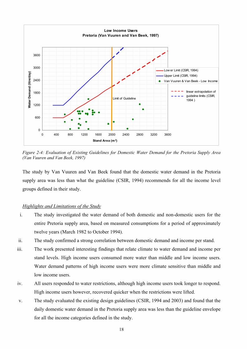
18
Low Income UsersPretoria (Van Vuuren and Van Beek, 1997)
0
600
1200
1800
2400
3000
3600
0 400 800 1200 1600 2000 2400 2800 3200 3600
Stand Area (m 2)
Wat
er D
eman
d (li
tre/
day)
Low er Limit (CSIR, 1994)
Upper Limit (CSIR, 1994)
Van Vuuren & Van Beek - Low Income
Limit of Guideline
linear extrapolation of guideline limits (CSIR, 1994 )
Figure 2-4: Evaluation of Existing Guidelines for Domestic Water Demand for the Pretoria Supply Area (Van Vuuren and Van Beek, 1997)
The study by Van Vuuren and Van Beek found that the domestic water demand in the Pretoria
supply area was less than what the guideline (CSIR, 1994) recommends for all the income level
groups defined in their study.
Highlights and Limitations of the Study
i. The study investigated the water demand of both domestic and non-domestic users for the
entire Pretoria supply area, based on measured consumptions for a period of approximately
twelve years (March 1982 to October 1994).
ii. The study confirmed a strong correlation between domestic demand and income per stand.
iii. The work presented interesting findings that relate climate to water demand and income per
stand levels. High income users consumed more water than middle and low income users.
Water demand patterns of high income users were more climate sensitive than middle and
low income users.
iv. All users responded to water restrictions, although high income users took longer to respond.
High income users however, recovered quicker when the restrictions were lifted.
v. The study evaluated the existing design guidelines (CSIR, 1994 and 2003) and found that the
daily domestic water demand in the Pretoria supply area was less than the guideline envelope
for all the income categories defined in the study.

19
vi. With the evaluation of the existing guidelines, the majority group with regards to income in a
supply area was determined and the average AADD and average stand are for the group was
determined.
vii. Non-domestic water demand was found not to be sensitive to climate (temperature and
rainfall) for the non-domestic users investigated in this study.
viii. The study had limitations with regards to the data accuracy of some parameters, such as the
meter reading intervals and land use characteristics.
ix. Income levels were defined and users categorised by means of property tax information.
x. The study was limited to formal residential developments with per stand water connections
and water-borne sanitation. Informal residential settlements are excluded from the study.
xi. It is of note that stand areas for the low income category considered with this work were
significantly greater (ranging from 600 to 2 900 m2) than those stand areas considered by
Stephenson and Turner (1996) for the low income category, which ranged from 200 – 400
m2.
2.2.4 Veck and Bill (2000)
Veck and Bill undertook a study for the Water Research Commission of South Africa in 2000 to
investigate the estimation of the price elasticity of residential water demand for different income
groups. They approached the problem of estimating the price elasticity of residential water demand
using a Contingent Valuation Method or model (CVM). Contingent evaluation models are models
where the input data is obtained by means of a survey to acquire perceived information from
individuals (users). In social-psychological terms it is a measure of behavioural intention. In the
case of this study, willingness to pay for water at increased tariffs was used as an indicator of these
behavioural intentions. A CVM is valuable in areas where data on the parameters that influence
water demand is limited. The results of this approach are not as reliable or accurate as actual
measured responses.
The researchers conducted the study in Alberton and Thokoza. In Alberton, 111 users were
interviewed and 50 users in Thokoza. The study comprised a two-stage survey. The objective of
the first stage of the survey was to obtain water demand profiles of the different users groups being
investigated. The second stage involved the acquisition of Contingent Values (i.e. answers to the
questions such as how much water the users would buy if the price increased). The study indicated
that the price of water was an important consideration so far as domestic consumption was
concerned. The authors found that the residential water demand in the study area had a negative
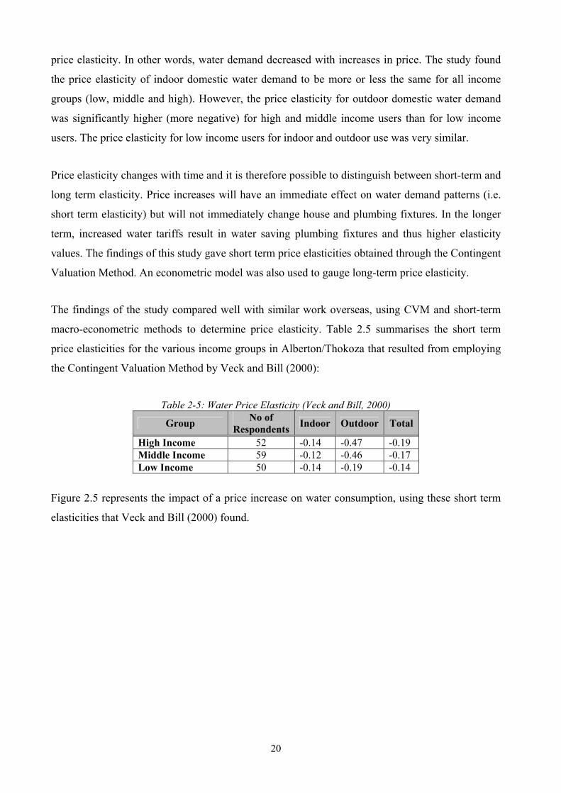
20
price elasticity. In other words, water demand decreased with increases in price. The study found
the price elasticity of indoor domestic water demand to be more or less the same for all income
groups (low, middle and high). However, the price elasticity for outdoor domestic water demand
was significantly higher (more negative) for high and middle income users than for low income
users. The price elasticity for low income users for indoor and outdoor use was very similar.
Price elasticity changes with time and it is therefore possible to distinguish between short-term and
long term elasticity. Price increases will have an immediate effect on water demand patterns (i.e.
short term elasticity) but will not immediately change house and plumbing fixtures. In the longer
term, increased water tariffs result in water saving plumbing fixtures and thus higher elasticity
values. The findings of this study gave short term price elasticities obtained through the Contingent
Valuation Method. An econometric model was also used to gauge long-term price elasticity.
The findings of the study compared well with similar work overseas, using CVM and short-term
macro-econometric methods to determine price elasticity. Table 2.5 summarises the short term
price elasticities for the various income groups in Alberton/Thokoza that resulted from employing
the Contingent Valuation Method by Veck and Bill (2000):
Table 2-5: Water Price Elasticity (Veck and Bill, 2000)
Group No of Respondents Indoor Outdoor Total
High Income 52 -0.14 -0.47 -0.19 Middle Income 59 -0.12 -0.46 -0.17 Low Income 50 -0.14 -0.19 -0.14
Figure 2.5 represents the impact of a price increase on water consumption, using these short term
elasticities that Veck and Bill (2000) found.

21
0
1
2
3
4
5
6
7
High IncomeIndoor Demand
High IncomeOutdoorDemand
Middle IncomeIndoor Demand
Middle IncomeOutdoorDemand
Low IncomeIndoor Demand
Low IncomeOutdoorDemand
Decr
ease
in W
ater
Con
sum
ptio
n (k
l/hou
seho
ld)
50% increase in price100% increase in price150% increase in price
Figure 2-5: Effect of an Increase in Water Price on Water Demand (Veck and Bill, 2000)
Veck and Bill found, with a macro-econometric model, that the long term price elasticity in the
study area for all income groups was -0.73. Compared to the average short term elasticity obtained
with the study, it gave an indication of how much more price increases could affect water demand
in the long term.
Veck and Bill also investigated the water demand profile of the users in the study area, not through
direct measurement of water consumption but through the Contingent Valuation Method. The
results can thus be termed perceived water demand of the users. The results of their study in this
regard are presented below in Table 2.6.
Table 2-6: Perceived Water Usage for Various Income Groups (Veck and Bill, 2000)
Group Perceived Water
Demand (kL/month) Perceived Water Demand
(litres/day) Alberton Middle Income 23 756 Alberton High Income 28 921 Thokoza Low Income 20 658
Highlights and Limitations of the Study
i. The study by Veck and Bill is one of the first of its kind in South Africa, investigating the
impact of price on water demand using a Contingent Valuation Method.
ii. The results of the study compared well with similar studies undertaken overseas.
iii. The study indicated that the price elasticity of water demand was negative, which implied that
if water prices increased, demand would decrease. An interesting finding was that the outdoor
demand was more price elastic than indoor demand for high and middle income groups. This
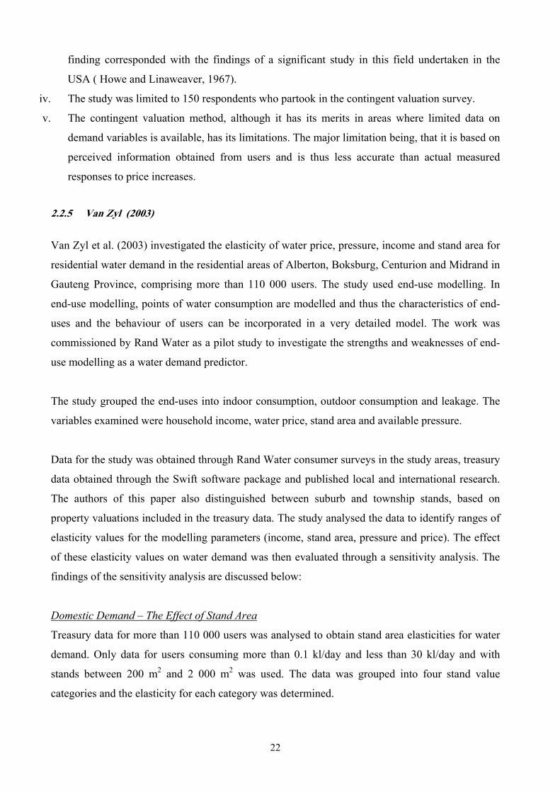
22
finding corresponded with the findings of a significant study in this field undertaken in the
USA ( Howe and Linaweaver, 1967).
iv. The study was limited to 150 respondents who partook in the contingent valuation survey.
v. The contingent valuation method, although it has its merits in areas where limited data on
demand variables is available, has its limitations. The major limitation being, that it is based on
perceived information obtained from users and is thus less accurate than actual measured
responses to price increases.
2.2.5 Van Zyl (2003)
Van Zyl et al. (2003) investigated the elasticity of water price, pressure, income and stand area for
residential water demand in the residential areas of Alberton, Boksburg, Centurion and Midrand in
Gauteng Province, comprising more than 110 000 users. The study used end-use modelling. In
end-use modelling, points of water consumption are modelled and thus the characteristics of end-
uses and the behaviour of users can be incorporated in a very detailed model. The work was
commissioned by Rand Water as a pilot study to investigate the strengths and weaknesses of end-
use modelling as a water demand predictor.
The study grouped the end-uses into indoor consumption, outdoor consumption and leakage. The
variables examined were household income, water price, stand area and available pressure.
Data for the study was obtained through Rand Water consumer surveys in the study areas, treasury
data obtained through the Swift software package and published local and international research.
The authors of this paper also distinguished between suburb and township stands, based on
property valuations included in the treasury data. The study analysed the data to identify ranges of
elasticity values for the modelling parameters (income, stand area, pressure and price). The effect
of these elasticity values on water demand was then evaluated through a sensitivity analysis. The
findings of the sensitivity analysis are discussed below:
Domestic Demand – The Effect of Stand Area
Treasury data for more than 110 000 users was analysed to obtain stand area elasticities for water
demand. Only data for users consuming more than 0.1 kl/day and less than 30 kl/day and with
stands between 200 m2 and 2 000 m2 was used. The data was grouped into four stand value
categories and the elasticity for each category was determined.
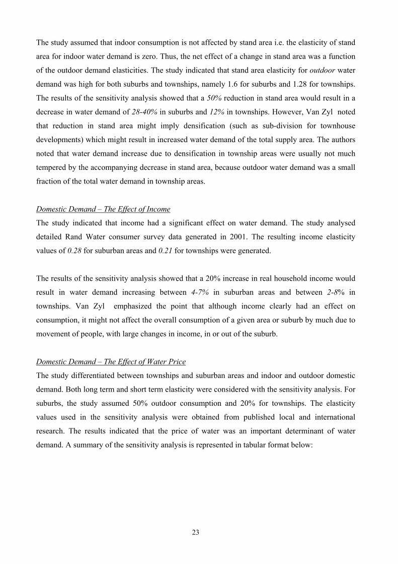
23
The study assumed that indoor consumption is not affected by stand area i.e. the elasticity of stand
area for indoor water demand is zero. Thus, the net effect of a change in stand area was a function
of the outdoor demand elasticities. The study indicated that stand area elasticity for outdoor water
demand was high for both suburbs and townships, namely 1.6 for suburbs and 1.28 for townships.
The results of the sensitivity analysis showed that a 50% reduction in stand area would result in a
decrease in water demand of 28-40% in suburbs and 12% in townships. However, Van Zyl noted
that reduction in stand area might imply densification (such as sub-division for townhouse
developments) which might result in increased water demand of the total supply area. The authors
noted that water demand increase due to densification in township areas were usually not much
tempered by the accompanying decrease in stand area, because outdoor water demand was a small
fraction of the total water demand in township areas.
Domestic Demand – The Effect of Income
The study indicated that income had a significant effect on water demand. The study analysed
detailed Rand Water consumer survey data generated in 2001. The resulting income elasticity
values of 0.28 for suburban areas and 0.21 for townships were generated.
The results of the sensitivity analysis showed that a 20% increase in real household income would
result in water demand increasing between 4-7% in suburban areas and between 2-8% in
townships. Van Zyl emphasized the point that although income clearly had an effect on
consumption, it might not affect the overall consumption of a given area or suburb by much due to
movement of people, with large changes in income, in or out of the suburb.
Domestic Demand – The Effect of Water Price
The study differentiated between townships and suburban areas and indoor and outdoor domestic
demand. Both long term and short term elasticity were considered with the sensitivity analysis. For
suburbs, the study assumed 50% outdoor consumption and 20% for townships. The elasticity
values used in the sensitivity analysis were obtained from published local and international
research. The results indicated that the price of water was an important determinant of water
demand. A summary of the sensitivity analysis is represented in tabular format below:
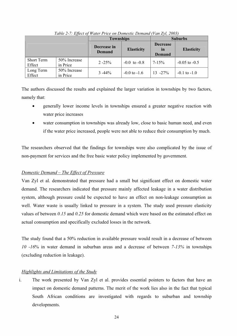
24
Table 2-7: Effect of Water Price on Domestic Demand (Van Zyl, 2003) Townships Suburbs
Decrease in Demand Elasticity
Decrease in
Demand Elasticity
Short Term Effect
50% Increase in Price 2 -25% -0.0 to -0.8 7-15% -0.05 to -0.5
Long Term Effect
50% Increase in Price 3 -44% -0.0 to -1.6 13 -27% -0.1 to -1.0
The authors discussed the results and explained the larger variation in townships by two factors,
namely that:
generally lower income levels in townships ensured a greater negative reaction with
water price increases
water consumption in townships was already low, close to basic human need, and even
if the water price increased, people were not able to reduce their consumption by much.
The researchers observed that the findings for townships were also complicated by the issue of
non-payment for services and the free basic water policy implemented by government.
Domestic Demand – The Effect of Pressure
Van Zyl et al. demonstrated that pressure had a small but significant effect on domestic water
demand. The researchers indicated that pressure mainly affected leakage in a water distribution
system, although pressure could be expected to have an effect on non-leakage consumption as
well. Water waste is usually linked to pressure in a system. The study used pressure elasticity
values of between 0.15 and 0.25 for domestic demand which were based on the estimated effect on
actual consumption and specifically excluded losses in the network.
The study found that a 50% reduction in available pressure would result in a decrease of between
10 -16% in water demand in suburban areas and a decrease of between 7-13% in townships
(excluding reduction in leakage).
Highlights and Limitations of the Study
i. The work presented by Van Zyl et al. provides essential pointers to factors that have an
impact on domestic demand patterns. The merit of the work lies also in the fact that typical
South African conditions are investigated with regards to suburban and township
developments.

25
ii. The study is limited to a pilot study and the aim was not to develop a comprehensive model
of domestic demand. Potential parameters influencing water demand such as climate,
geographic location, level of service and age of infrastructure were not considered in the
analysis.
iii. Although the study focused on a restricted number of variables in Gauteng only, the results
can serve as general markers to parameters that influence water demand.
iv. The study indicated that price had the most significant impact on domestic water demand
patterns.
v. Household income, stand area and pressure had positive demand elasticities, i.e. an increase
in income, stand area or pressure resulted in an increased water demand.
vi. The study indicated the strengths and weaknesses of end-use modelling and reported on its
potential application in South Africa
vii. The sensitivity analysis was limited to one factor at a time and although useful in
highlighting the impact of the individual parameters, it cannot be used to estimate the
combined effects of different user types and parameters.
viii. The end-use model was limited to two types of domestic users namely suburban and
townships. Additional user categories such as parks, schools, business commercial sites etc.
had not been considered.
2.2.6 Jacobs (2004) The work by Jacobs et al. presents a valuable discussion with regards to estimating residential
water demand in southern Africa using a single-coefficient model that relates water demand with
stand area. The study analysed the measured water consumption of 582 997 single residential
stands in various towns and cities in southern Africa by using treasury databases. The following
municipalities were investigated:
Ekurhuleni Metropolitan Municipality: Alberton, Thokoza, Benoni, Daveyton, Etwatwa,
Boksburg, Vosloorus, Brakpan, Germiston, Katlehong,, Kempton Park, Tembisa, Springs,
Kwa-Thema
Cape Town: Blaauwberg, Helderberg, Tygerberg (West, Central and South)
Tshwane (Gauteng): Akasia, Atteridgeville, Centurion, Mamelodi, Pretoria, Soshanguve,
Randfontein
Johannesburg: Midrand
George
Windhoek (Namibia)

26
The study analysed consumption data of at least 12 months varying from December 1999 to July
2003 for only single residential stands, with one water meter per stand (and vice versa) and using
less than 20 kl per day. Only stands with areas between 50 m2 and 2 050 m2 were used in the study.
For the Ekurhuleni dataset the stands are categorised as either “suburban” or “township”. This
classification was made by viewing the treasury records with SG (Surveyor General) cadastral
information in GIS (Geographic Information System) format and then classifying the stands as
suburban or township based on knowledge of the areas.
Domestic Demand – Effect of Stand area
The researchers of this paper proved that a strong relationship exists between domestic AADD
(Annual Average Daily Demand) and stand area. Although the work acknowledged that numerous
factors influence water demand, stand area is used as a single explanatory variable in the model.
The authors noted that a model based on stand area alone has limited application and should be
used only when better estimation methods are not available. The study presented three unique
models for three Southern African geographic regions that could be used to estimate the AADD for
single residential stands, namely:
Coastal winter rainfall region
Inland summer rainfall region (for suburban and township developments separately)
Coastal all-year rainfall region
For each model, a guideline curve and an upper and a lower envelope curve are presented. Figures
2.6, 2.7, 2.8 and 2.9 represent the three models and their guideline curves and also compares the
curves with the existing “Red Book” guidelines. This investigation found that the “Red Book”
guidelines were too conservative, leading to possible over-design and potential unnecessary
expenditure by water authorities.

27
0
600
1200
1800
2400
3000
3600
0 400 800 1200 1600 2000
Stand Area (m2)
Wat
er D
eman
d (li
tre/d
ay/s
tand
)
Red Book Red Low er Limit (CSIR 2003)
Red Book Upper Limit (CSIR 2003)
Jacobs et al Upper Limit
Jacobs et al Low er Limit
Jacobs et al Guideline
Figure 2-6: Southern African Coastal Winter Rainfall Region Model (Suburban and Townships) (Jacobs, 2004) Jacobs et al. compared their findings with other work that evaluated residential domestic demand.
The results of Jacobs et al. compared very well with the findings of Stephenson and Turner (1996),
Van Zyl (2003) and a similar study in Windhoek (Water Transfer Consultants 2001, WCE et al.,
2003).
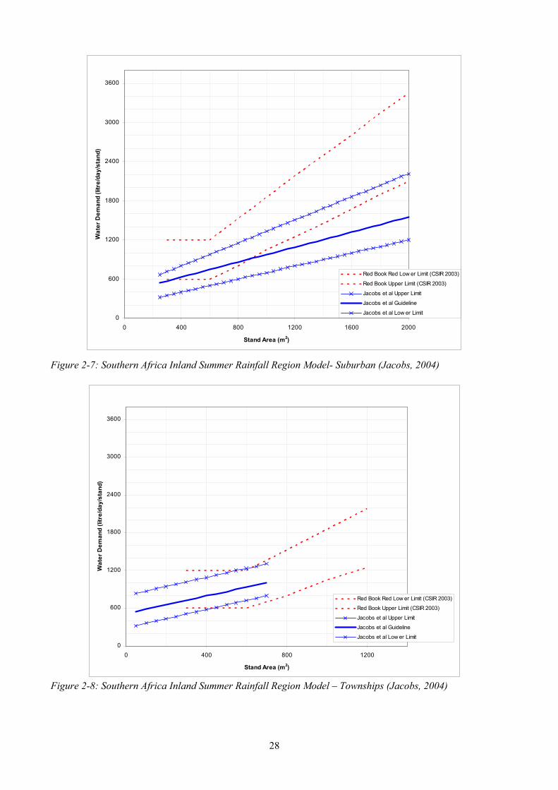
28
0
600
1200
1800
2400
3000
3600
0 400 800 1200 1600 2000
Stand Area (m2)
Wat
er D
eman
d (li
tre/
day/
stan
d)
Red Book Red Low er Limit (CSIR 2003)
Red Book Upper Limit (CSIR 2003)
Jacobs et al Upper Limit
Jacobs et al Guideline
Jacobs et al Low er Limit
Figure 2-7: Southern Africa Inland Summer Rainfall Region Model- Suburban (Jacobs, 2004)
0
600
1200
1800
2400
3000
3600
0 400 800 1200
Stand Area (m2)
Wat
er D
eman
d (li
tre/
day/
stan
d)
Red Book Red Low er Limit (CSIR 2003)
Red Book Upper Limit (CSIR 2003)
Jacobs et al Upper Limit
Jacobs et al Guideline
Jacobs et al Low er Limit
Figure 2-8: Southern Africa Inland Summer Rainfall Region Model – Townships (Jacobs, 2004)
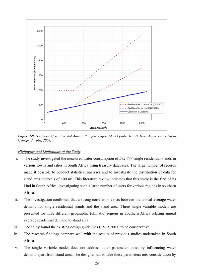
29
0
600
1200
1800
2400
3000
3600
0 400 800 1200 1600 2000
Stand Area (m2)
Wat
er D
eman
d (li
tre/
day/
stan
d)
Red Book Red Low er Limit (CSIR 2003)
Red Book Upper Limit (CSIR 2003)
Jacobs et al Guideline
Figure 2-9: Southern Africa Coastal Annual Rainfall Region Model (Suburban & Townships) Restricted to George (Jacobs, 2004)
Highlights and Limitations of the Study
i. The study investigated the measured water consumption of 582 997 single residential stands in
various towns and cities in South Africa using treasury databases. The large number of records
made it possible to conduct statistical analyses and to investigate the distribution of data for
stand area intervals of 100 m2. This literature review indicates that this study is the first of its
kind in South Africa, investigating such a large number of users for various regions in southern
Africa.
ii. The investigation confirmed that a strong correlation exists between the annual average water
demand for single residential stands and the stand area. Three single variable models are
presented for three different geographic (climatic) regions in Southern Africa relating annual
average residential demand to stand area.
iii. The study found the existing design guidelines (CSIR 2003) to be conservative.
iv. The research findings compare well with the results of previous studies undertaken in South
Africa.
v. The single variable model does not address other parameters possibly influencing water
demand apart from stand area. The designer has to take these parameters into consideration by
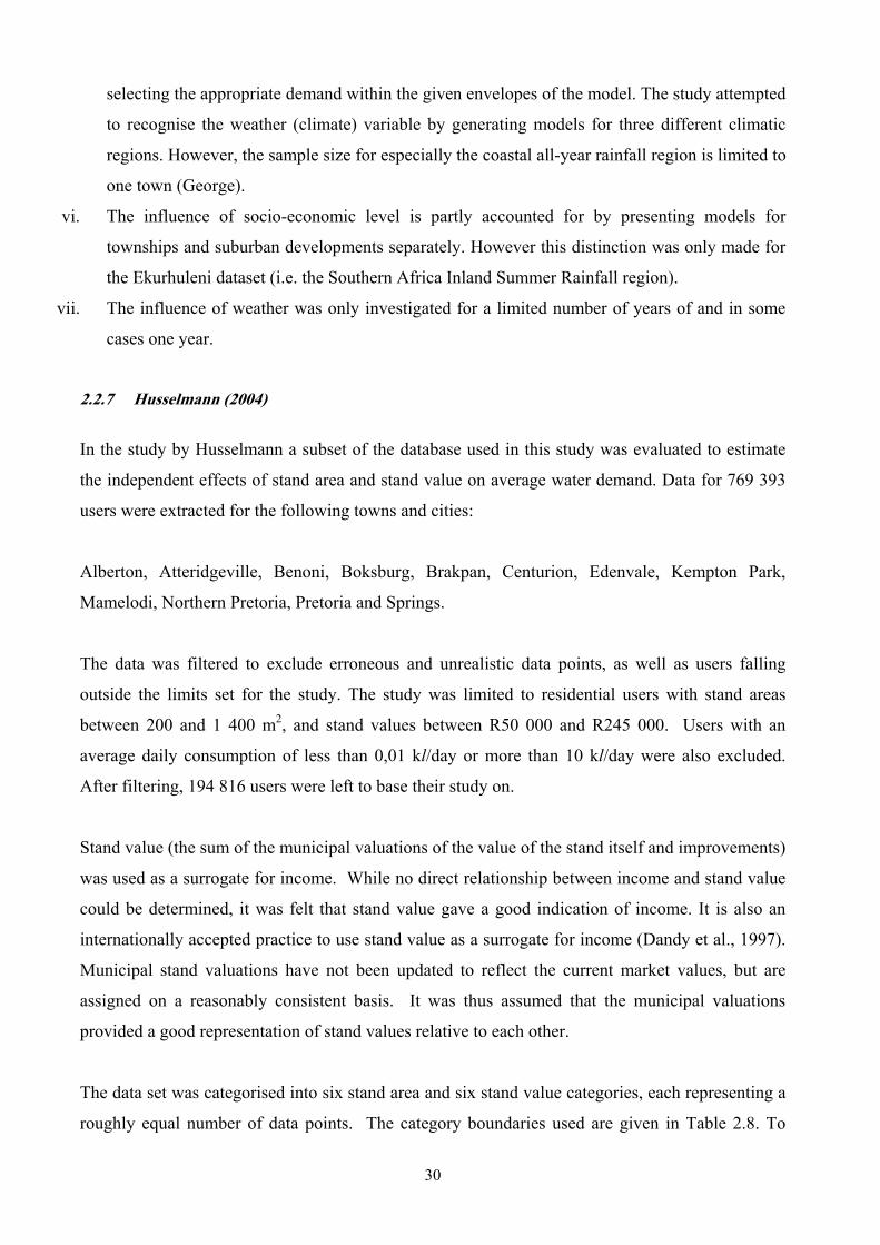
30
selecting the appropriate demand within the given envelopes of the model. The study attempted
to recognise the weather (climate) variable by generating models for three different climatic
regions. However, the sample size for especially the coastal all-year rainfall region is limited to
one town (George).
vi. The influence of socio-economic level is partly accounted for by presenting models for
townships and suburban developments separately. However this distinction was only made for
the Ekurhuleni dataset (i.e. the Southern Africa Inland Summer Rainfall region).
vii. The influence of weather was only investigated for a limited number of years of and in some
cases one year.
2.2.7 Husselmann (2004)
In the study by Husselmann a subset of the database used in this study was evaluated to estimate
the independent effects of stand area and stand value on average water demand. Data for 769 393
users were extracted for the following towns and cities:
Alberton, Atteridgeville, Benoni, Boksburg, Brakpan, Centurion, Edenvale, Kempton Park,
Mamelodi, Northern Pretoria, Pretoria and Springs.
The data was filtered to exclude erroneous and unrealistic data points, as well as users falling
outside the limits set for the study. The study was limited to residential users with stand areas
between 200 and 1 400 m2, and stand values between R50 000 and R245 000. Users with an
average daily consumption of less than 0,01 kl/day or more than 10 kl/day were also excluded.
After filtering, 194 816 users were left to base their study on.
Stand value (the sum of the municipal valuations of the value of the stand itself and improvements)
was used as a surrogate for income. While no direct relationship between income and stand value
could be determined, it was felt that stand value gave a good indication of income. It is also an
internationally accepted practice to use stand value as a surrogate for income (Dandy et al., 1997).
Municipal stand valuations have not been updated to reflect the current market values, but are
assigned on a reasonably consistent basis. It was thus assumed that the municipal valuations
provided a good representation of stand values relative to each other.
The data set was categorised into six stand area and six stand value categories, each representing a
roughly equal number of data points. The category boundaries used are given in Table 2.8. To
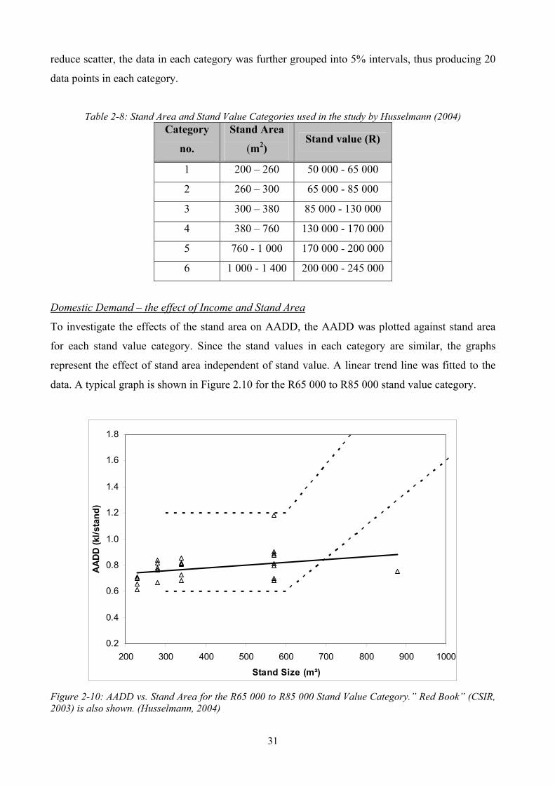
31
reduce scatter, the data in each category was further grouped into 5% intervals, thus producing 20
data points in each category.
Table 2-8: Stand Area and Stand Value Categories used in the study by Husselmann (2004) Category
no.
Stand Area
(m2) Stand value (R)
1 200 – 260 50 000 - 65 000
2 260 – 300 65 000 - 85 000
3 300 – 380 85 000 - 130 000
4 380 – 760 130 000 - 170 000
5 760 - 1 000 170 000 - 200 000
6 1 000 - 1 400 200 000 - 245 000
Domestic Demand – the effect of Income and Stand Area
To investigate the effects of the stand area on AADD, the AADD was plotted against stand area
for each stand value category. Since the stand values in each category are similar, the graphs
represent the effect of stand area independent of stand value. A linear trend line was fitted to the
data. A typical graph is shown in Figure 2.10 for the R65 000 to R85 000 stand value category.
0.2
0.4
0.6
0.8
1.0
1.2
1.4
1.6
1.8
200 300 400 500 600 700 800 900 1000
Stand Size (m²)
AAD
D (k
l/sta
nd)
Figure 2-10: AADD vs. Stand Area for the R65 000 to R85 000 Stand Value Category.” Red Book” (CSIR, 2003) is also shown. (Husselmann, 2004)
32
The trend lines for each of the six stand value categories were then plotted on the same axes as
shown in Figure 2.11. The Red Book minimum and maximum guideline values are also shown.
Figure 2.11 shows a clear relationship between AADD and stand area for all the stand value
categories, with the AADD increasing with increasing stand area. The higher the stand value, the
greater the AADD for the same stand area. This relationship can also be shown by plotting AADD
against stand value for the different stand area categories. However, stand value is a subjective
measure, likely to vary between municipal areas and with time. The authors thus felt that stand
area was the better indicator of the demand envelope, with stand value (or income) playing a part
in determining the relative position of a given supply area between the upper and lower bounds.
0.2
0.4
0.6
0.8
1.0
1.2
1.4
1.6
1.8
200 400 600 800 1000 1200
Stand Size (m²)
AADD
(kl/s
tand
)
Red Book 50-65 65-85 85-130130-170 170-200 200-245
Stand value category (R1000)
Figure 2-11: AADD as a Function of Stand Area for Different Stand Value Categories (Husselmann, 2004)
It can also be noted from Figure 2.11 that the higher the stand value, the smaller is the slope of the
AADD vs. stand area trend line. The researchers therefore argued that this is directly opposed to
the implicit assumption in the Red Book graph, which increases the slope for larger stand areas.
Finally, the authors indicated that while the AADD values for smaller stands fall within the “Red
Book” guideline values, the “Red Book” possibly overestimated the AADD for larger stands. In

33
this study, for stands larger than 800 m2, the trend lines fell below even the minimum envelope line
proposed by the Red Book.
The authors propose a new design envelope for AADD. To provide a better estimate of the AADD
Husselmann plotted all the datapoints on which the lines in Figure 2.11 were based on a graph
showing the Red Book Guideline envelopes (Figure 2.12). Husselman’s new proposed envelope is
also shown in Figure 2.12. This curve differs substantially from the Red Book graph in terms of
the slopes and values of the envelope lines. The inflection points of the envelope lines remain at a
stand area of 600 m2, but their slopes decrease rather than increase. The proposed minimum
AADD limit is lower than that of the Red Book for all stand areas. The proposed maximum
AADD limit exceeds that of the Red Book for stand areas between 300 and 700 m2, but is lower
for the rest. Significantly, its maximum line is lower than even the minimum Red Book line for
stand areas exceeding 1 050 m2. This represents a substantial reduction in design AADD for larger
stands and will have a marked impact on the cost of providing water supply infrastructure for these
areas.
(200; 1.1)
(1400; 1.9)
(600; 1.5)
(200; 0.2)
(600; 0.5)(1400; 0.60)
0.0
0.2
0.4
0.6
0.8
1.0
1.2
1.4
1.6
1.8
2.0
0 200 400 600 800 1000 1200 1400
Stand Size (m²)
AADD
(kl/s
tand
)
Red Book 50-65 65-85 85-130130-170 170-200 200-245 Proposed
Stand value category (R1000)
Figure 2-12: Proposed New Design Envelope for AADD showing data points and the Red Book Envelopes (Husselmann, 2004)

34
Highlights and Limitations of the Study
i. The study investigated measured consumption data for 769 393 residential stands in Gauteng.
ii. The data was divided into six stand area and six stand value categories to investigate the
independent effects of stand value and size on water demand.
iii. The study found that there is a definite trend of increasing water demand with increases in both
stand area and stand value (and thus income).
iv. It was concluded that stand area is a good measure for defining an AADD range. The design
engineer should use information such as income, climate, level of living and other relevant
information to determine an appropriate AADD within the minimum and maximum range.
v. It was shown that increasing stand value increased the AADD (and thus moved it closer to the
upper AADD range), and also reduced the slope of the curve.
vi. A comparison of the results with the proposed Red Book (CSIR 2003) guidelines for water
demand showed that the Red Book guideline could underestimate the AADD in the 300 to 700
m2 stand area range, but overestimate the AADD for stand areas larger than 700 m2. A new
envelope curve for estimating AADD is proposed based on the data analysed.
2.3 Summary of Major Unresolved Problems i. The review of previous work done in South Africa indicates that the following are
significant parameters that affect domestic water demand:
Stand area
Household income
Water Price
Available Pressure
Type of development (suburban vs. township)
Climate
These findings provided a base for the further work undertaken in this study.
ii. Some work has been done on the influence of climate. The study by Van Vuuren and Van
Beek (1997) presented interesting findings regarding the combined effect of climate and
income but was limited to the Pretoria supply area (one climatic region) and did not
consider typical township developments. Jacobs et al. (2004) considered the influence of
climate on domestic water demand for three climatic regions but only with regards to stand
area in a single variable model. Garlipp conducted a meticulous study on the effect of
climate on domestic water demand, but considered cities as a whole (i.e. the water demand
for a city was evaluated against climate). This study investigates the effect of climate for

35
individual water consumers for various user categories in various types of developments
(city vs. small towns) in various climatic regions in South Africa.
iii. Most of the previous work reviewed considered parameters influencing water demand
individually. This literature review indicates that research of non-domestic demand patterns
is very limited. This study investigates non-domestic water demand and the possible
parameters influencing non-domestic water demand for a cross selection of South African
towns and cities for various non-domestic user categories.
iv. Most of the studies considered with this review, were undertaken in the Gauteng area. Only
the work by Jacobs et al. (2004) considered different geographic regions in Southern Africa
and the study by Garlipp (1979) considered other cities and regions in South Africa.
However the study by Jacobs et al. (2004) considered a single variable namely stand area.
Although Garlipp’s (1979) work is very valuable in this regard it was undertaken nearly 30
years ago and a lot has changed in the socio-economic and political characteristics of the
country. This study investigates water users across South Africa in recent years (1998 –
2005) and considered a number of possible parameters influencing water demand.
v. Apart from the study of Jacobs et al. (2004) that investigated nearly 600 000 domestic users
country wide, the study by Van Zyl et al. (2003) that investigated 110 000 domestic users
and the study by Husselmann (2004) with nearly 800 000 users, the other studies
investigated a limited number of users. A large number of records make it possible to
conduct meticulous statistical analyses and to investigate the distribution of data in greater
detail and to possibly have more representative samples of specific data characteristics.
This study has extracted consumption data for more than 2.5 million users.
vi. The literature review indicates that the existing design guidelines (The “Red Book”) (CSIR,
2003) may be conservative (Jacobs et al., 2004; Husselmann, 2004; Van Vuuren and Van
Beek, 1997).
36
3 THE DATA
3.1 Introduction
Good quality data is always hard to come by and this is also the case with water consumption
records. Even a large logging exercise, apart from being expensive, cannot realistically aim to
reach a statistically reliable sample of households. This study considered municipal meter readings
as an ideal source for water consumption information since the readings are taken on a regular
basis by virtually all municipalities in the country. However, this information is generally difficult
to access and are typically discarded (and thus lost) after a short period of time.
In recent years, GLS Consulting Engineers developed a software product called Swift. This
product allows the user to access municipal treasury databases to obtain demographic and water
consumption information for large numbers of users (domestic and non-domestic). Swift has been
implemented by many local authorities throughout South Africa, covering different economic,
socio-economic, climatic and other regions.
This study is based on water consumption data extracted from various Swift databases developed
for different municipalities throughout the country. The data reflects municipal water meter
readings used for customer billing and thus also included errors present in these databases.
Verification steps were taken to minimise the number of errors present in the analysis. The data
cleaning process is discussed in detail in the following section.
Data on climatic and socio-economic parameters that possibly influence water consumption was
sourced from the South African Weather Service and the South African Demarcation Board. The
process of linking this data to the Swift data sets is also described in this chapter.
3.2 Water Consumption Data
3.2.1 Data Collection
Municipal treasury data for a number of municipalities was collected in January to May 2005 from
various Swift databases operated by GLS Consulting Engineers. An on-site survey was required to
establish which municipal treasury databases were available for extraction. Furthermore a
complete understanding of the Swift software was necessary in order to understand what Swift
offered in terms of data. The data storing and primary data cleaning mechanisms had to be clearly
37
understood to ensure that the final data extracted was what was needed for the study and that it was
as accurate as possible.
The data extracted from the Swift databases covers a time period of eight years (1998 – 2005) and
consequently the data was available in various versions of Swift. The automation process could not
be altogether automated since the data was sourced from various municipalities that used different
coding systems that had to be standardised in Swift. Each database had to be thoroughly checked
after extraction to ensure all the relevant data was included. This study made use of Microsoft
Access to analyse and store the data. The water consumption and related data thus had to be
exported from the Swift databases in a readable format (PARADOX). Some Swift data was very
easily extracted but other information such as the municipal land use codes and the assignment of
these codes to the standard Swift land use codes was more complicated and required interpretation
and checking after each extraction.
After extraction and importing the data into Microsoft Access format a preliminary assessment of
the data was done to ascertain whether there was any missing data for specific towns or
municipalities. The reasons for the missing data were investigated. For example, is the treasury
data simply not populated in the databases of is it available in another format or another database?
If the missing data was not available an assessment was made on the impact this might have on the
affected datasets and the subsequent analyses. If the impact was likely to be significant the affected
datasets were discarded. For example if the land use codes were not populated, this would have a
significant impact on further analysis and the data would thus be discarded.
The treasury data extracted with Swift contained the following information per water meter that
was used in the research:
Unique identifier
Municipality
Town
Stand area
Stand Value (R)
Value of Improvement on the stand (R)
Land use code
Suburb
Zoning codes

38
Water meter information (meter registration number, installation date, measurement unit)
Flag whether vacant or not
Flag whether large user or not
Number of units (in the case of group housing)
Water meter reading dates
Monthly water meter readings
Number of readings
Calculated AADD (Annual Average Daily Demand) (kl/day)
Adjustment codes (where data have been manipulated by Swift procedures)
3.2.2 Description of the Data
Forty eight (48) municipal treasury databases were collected and extracted for further analysis in
this study. This includes 4 metros (Johannesburg, Tshwane, Ekurhuleni and Cape Town) and 151
cities and towns. Table 3.1 lists the municipalities studied, the period of water consumption
monitoring, and the total number of stands (uncleaned) for each municipality.
Table 3-1: Summary of Municipal Treasury Data Used. Municipality Towns and Cities Period of Readings # of Stands
Beaufort West Beaufort West Dec 02 - Feb 04 6 941
BergRiver Velddrif, Porterville, Piketberg, Laaiplek, Aurora, Eendekuil, Dwarskersbos, Redelingshuys Feb 03 - Mar 04 10 012
Blaauwberg Blaauwberg, Milnerton, Mamre, Atlantis, Melkbos Jun 00 - Jul 02 49 298 Breede River Robertson, Bonnievale, Ashton, Montagu, McGregor Oct 02 - Oct 04 20 079 Breede Valley Worcester Nov 99 - Jan 04 15 075 Buffalo City East London Jan 03 - Feb 05 119 748
Cape Agulhas Bredasdorp, Waenhuiskrans, Struisbaai, Suiderstrand, Napier, Klipdale, Lagulhas Mar 99 - Feb 04 8 576
Cederberg Clanwilliam, Citrusdal, Lamberts Bay, Graafwater, Elands Bay, Leipoldtville Dec 02 - Dec 03 6 881
Drakenstein Wellington, Paarl, Gouda, Bainskloof, Hermon, Mbekweni Dec 01 - Dec 03 37 076
Ekurhuleni Alberton Aug 02 - Sep 04 40 065 Ekurhuleni Germiston Aug 02 - Sep 04 117 846 Ekurhuleni Kempton Park Aug 02 - Sep 04 87 779 Ekurhuleni Lethabong Aug 02 - Sep 04 25 150 Ekurhuleni Nigel Sep 02 - Oct 04 27 420 Ekurhuleni Springs Sep 02 - Oct 04 45 461 Ekurhuleni Benoni Sep 02 - Oct 04 100 921 Ekurhuleni Boksburg Aug 02 - Sep 04 72 334 Ekurhuleni Brakpan Sep 02 - Oct 04 63 812
George George, Heroldsbay, Wildernis, Twee Rivieren Jul 99 - Jul 03 33 229 Helderberg Gordons Bay, Strand, Somerset West, Maccasar Apr 98 - Apr 03 37 830
Johannesburg Lethabong Feb 02 - Mar 04 6 398 Johannesburg Midrand Feb 02 - Mar 04 39 699

39
Municipality Towns and Cities Period of Readings # of Stands
Johannesburg Northern Johannesburg (Sandton, Randburg, Bryanston, Sunninghill, Morningside) Jan 02 - Feb 04 123 262
Johannesburg Southern Johannesburg 1 Feb 02 - Mar 04 96 235 Johannesburg Southern Johannesburg (Soweto) Feb 02 - Mar 04 160 076 Johannesburg Eastern Johannesburg Feb 02 -Mar 04 118 315 Johannesburg Western Johannesburg Feb 02-Mar 04 105 494
Langeberg Albertinia, Gouritsmond, Heidelberg, Jongensfontein, Riversdale, Slangrivier, Stilbaai, Theronsville, Witsand Dec 02 -Jan 04 16 008
Matzikama Klawer, Lutzville, Vanrhynsdorp, Vredendal Jan 02 - Feb 04 8 317 Mossel Bay Mossel Bay, Dana Bay, Klein Brak, Hartenbos Oct 01 - Oct 03 32 157 Oostenberg Brackenfell, Blue Downs, Kuilsrivier Nov 99 - Dec 01 61 300 Oudtshoorn Oudtshoorn Nov 01 - Nov 03 14 335 Overstrand Gansbaai, Hermanus, Kleinmond, Stanford Feb 00 -Feb 04 30 307
Plettenberg Bay Plettenberg Bay Dec 99 - Nov 04 9 155 Randfontein Randfontein, Mohlakeng Apr 01 - May 03 17 979
Saldanha Bay Langebaan, Paternoster, Jacobsbaai, Vredenburg, St Helena Bay, Hopefield, Ongegund, Louwville Apr 99 - Mar 04 23 481
Sedibeng Sharpeville, Sebokeng, Boipatong, Evaton, Stretford, Vereeniging, Meyerton, Kanana, Hartebeestfontein, Klipwater, Walkerville
June 02 - Jul 04 170 126
Stellenbosch Stellenbosch Oct 99 - Oct 01 14 335
Swartland Abbotsdale, Chatsworth, Grottobaai, Darling, Malmesbury, Morreesburg, Koringberg, Riebeeck Wes, Riebeeck Kstl, Yzerfontein
Oct 01 - Oct 03 22 763
Theewatersklf Caledon, Grabouw, Genadedal, Greyton, Riversonderend, Villiersdorp Sep 03 -Oct 04 16 305
Tshwane Atteridgeville Feb 2002 - Feb 2005 17 753 Tshwane Centurion Dec 2002 -Jan 2005 35 652 Tshwane Mamelodi Feb 2002 - Feb 2005 38 493 Tshwane NPMSS - Akasia, Rosslyn, Shoshanghuve Feb 2003 -Mar 2005 84 900 Tshwane Odi (Garankua) Dec 2002 - Mar 2005 45 793 Tshwane Pretoria Feb 2002 -Feb 2005 146 691 Tshwane Temba (Hammanskraal) Jan 2004 - Feb 2005 12 108
Tygerberg Bellville, Cape Town, Delft, Durbanville, Goodwood, Mfuleni, Khayelitsha, Parow Aug 2001 - Aug 03 196 036
TOTAL 2 589 006
Figure 3.1 portrays the location of each municipality that was studied and the major water regions
of South Africa. The water regions were proposed by Basson (1997) and published in a report by
the Department of Water Affairs and Forestry. The regions were created by grouping together
catchments of broadly similar hydrometeorological characteristics.
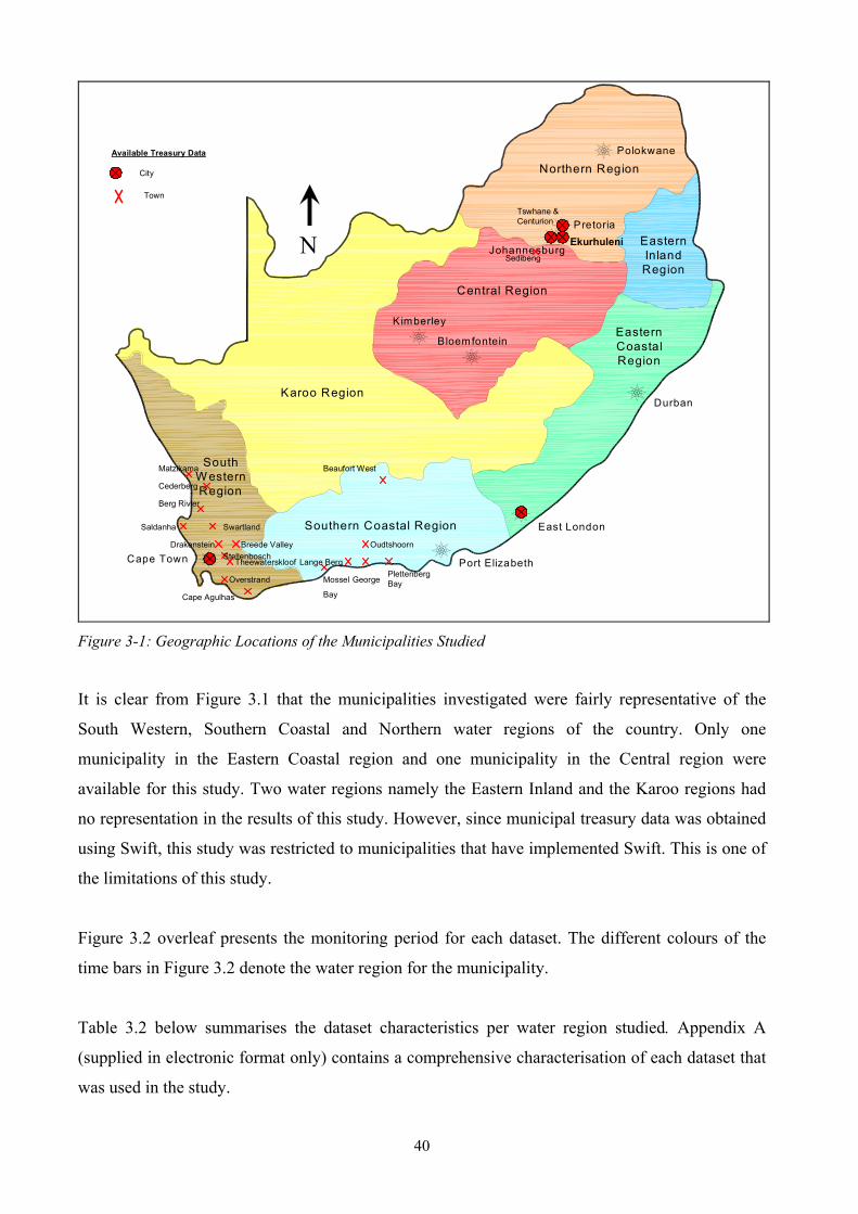
40
South W estern Region
Southern Coastal Region
Eastern Coastal Region
Central Region
Karoo Region
Northern Region
Eastern Inland Region
Cape Town
Bloemfontein
Durban
Port Elizabeth
East London
Kimberley
Polokwane
Pretoria
JohannesburgN
Beaufort West
Berg Rivier
Breede Valley
Cape Agulhas
Cederberg
Matzikama
Drakenstein
Ekurhuleni
Lange Berg
OverstrandPlettenberg Bay
Saldanha
Sedibeng
Swartland
Theewaterskloof
George
Tswhane & Centurion
Stellenbosch
Mossel
Bay
Oudtshoorn
City
Town
Available Treasury Data
Figure 3-1: Geographic Locations of the Municipalities Studied
It is clear from Figure 3.1 that the municipalities investigated were fairly representative of the
South Western, Southern Coastal and Northern water regions of the country. Only one
municipality in the Eastern Coastal region and one municipality in the Central region were
available for this study. Two water regions namely the Eastern Inland and the Karoo regions had
no representation in the results of this study. However, since municipal treasury data was obtained
using Swift, this study was restricted to municipalities that have implemented Swift. This is one of
the limitations of this study.
Figure 3.2 overleaf presents the monitoring period for each dataset. The different colours of the
time bars in Figure 3.2 denote the water region for the municipality.
Table 3.2 below summarises the dataset characteristics per water region studied. Appendix A
(supplied in electronic format only) contains a comprehensive characterisation of each dataset that
was used in the study.

41
Table 3-2: Summary of Dataset Characteristics per Water Region
Water Region (DWAF) (Basson ,
1997)
Municipalities Number of Data
Sets
Total Number of
Stands
Total Number of
Vacant Stands
Total Number
of Domestic
Stands
Total Number of Stands
with Unknown Land use
Central Sedibeng 1 170 126 129 357 144 135 8 081 Eastern Coastal Buffalo City (East London) 1 119 748 47 877 102 665 11 795
Northern Ekurhuleni, Johannesburg Water, Randfontein, Tshwane
24 1 629 636 697 706 1 377 457 155 784
South Western
BergRiver, Blaauwberg, Breede River, Breede Valley, Cape Agulhas, Cederberg, Drakenstein, Helderberg, Matzikama, Oostenberg, Overstrand, Saldanha Bay, Stellenbosch, Swartland, Theewaterskloof, Tygerberg
16 557 671 157 165 457 613 38 888
Southern Coastal
Beaufort West, George, Langeberg, Mossel Bay, Oudtshoorn, Plettenberg Bay
6 111 825 33 472 68 685 15 895
TOTAL 48 2 589 006 1 065 577 2 150 555 230 443

42
Anal
ysis
of R
eadi
ng P
erio
ds fo
r Eac
h W
ater
Reg
ion
Nov-97Jan-98Mar-98May-98
Jul-98Sep-98Nov-98Jan-99Mar-99May-99
Jul-99Sep-99Nov-99Jan-00Mar-00May-00
Jul-00Sep-00Nov-00Jan-01Mar-01May-01
Jul-01Sep-01Nov-01Jan-02Mar-02May-02
Jul-02Sep-02Oct-02Dec-02Feb-03Apr-03Jun-03Aug-03Oct-03Dec-03Feb-04Apr-04Jun-04Aug-04Oct-04Dec-04Feb-05Apr-05Jun-05Aug-05
Sed
iben
gB
uffu
lo C
ityE
kurh
ulen
iJo
hann
esbu
rg W
ater
Tshw
ane
Ran
dfon
tein
Ove
rstra
ndB
laau
wbe
rgO
oste
nber
gTy
gerb
erg
Ber
gRiv
erC
ape
Agu
lhas
Hel
derb
erg
Sal
danh
a B
ayB
reed
e R
iver
Bre
ede
Val
ley
Ced
erbe
rgD
rake
nste
inM
atzi
kam
aS
telle
nbos
chS
war
tland
Thee
wat
ersk
loof
Lang
eber
gG
eorg
eM
osse
l Bay
Ple
ttenb
erg
Bay
Bea
ufor
t Wes
tO
udts
hoor
n
12m
onth
s
Nor
ther
n
East
ern
Coa
stal
Sout
h W
este
rn
Cen
tral
Sout
hern
Coa
stal
Figu
re 3
-2: M
onito
ring
Per
iod
of E
ach
Dat
aset
Use
d in
the
Stud
y

43
The largest number of consumers investigated in this study was located in the Northern water
region. This group of consumers were all located in Gauteng and include the three metros of
Johannesburg, Tshwane and Ekurhuleni. The next largest group is situated in the South Western
region and includes the metro of Cape Town. A large number of stands (41% of the total number)
were assigned as ‘vacant’ stands in the treasury systems. Not all of these ‘vacant’ stands had zero
water consumption; quite a number had relevant and regular readings. It may be possible that
although these stands had at one time in the past been vacant, they had since been occupied, but
the treasury systems had not been updated. However, it was considered prudent to exclude all
stands that were flagged as vacant from further analysis even if some stands had relevant water
consumption records. This process is described in the following section (3.2.3).
This investigation relied heavily on the accuracy of the land use codes assigned by the treasury
systems. The land use codes were used to categorise the consumers in user type categories prior to
analysis. Where no land use code has been assigned (8.9% of the total number of stands) the data
was of no use in this study and was discarded.
3.2.3 Data Verification
The data used in this study was obtained from municipal meter readings entered into treasury
databases for billing purposes and then extracted using Swift. It was necessary to verify the data to
identify and eliminate potential errors in an objective manner. Various possible errors could be
included in the database, namely:
Wrong water meter readings;
Errors in entering the meter readings into the treasury database;
Errors in transferring the data to and from Swift;
Under- or over-registering of water meters;
Meters not read regularly;
Meter readings not taken on the same day of the month;
Missing or erroneous user data, such as stand area, stand value or suburb;
Incorrect land use assignment.

44
Primary Data Cleaning
The data collection process created a database for each municipality in Microsoft Access format
(48 databases). Before all the databases were consolidated into a single database, each municipal
database was subjected to a primary data cleaning procedure. The aim of the primary data cleaning
procedure was to eliminate records with obvious errors in the meter readings.
The primary data cleaning made use of the Swift adjustment codes. Swift assigns adjustment codes
to every treasury record during the process of calculation of water demand and the consolidation of
records. The adjustment codes describe the procedure of manipulation that was carried out on the
record by Swift in order to calculate an AADD value for the water meter. The primary data
cleaning process used these adjustment codes as a guideline to disregard or omit records from
further analysis. The table below lists the Swift adjustment codes and provides a description of the
meaning of the code (i.e. what action was carried out by Swift). The table indicates whether
records with specific adjustment codes were discarded in the primary data cleaning procedure or
not.
Table 3-3: Primary Data Cleaning Procedure Code No. Code Description Discard
Record? 1 None No readings were found for the erf. Yes 2 Single A single reading was found for the erf. Yes
3 Dates Inconsistent dates. The system could not determine the order in which the readings should be placed due to date inconsistencies. Both the AADD and TWD are set to 0.
Yes
4 Clock Clock overs. This is where the meters have clocked over. The system will manage this situation, given the display size of the meter. No
5 New Meter This is where the new meters have been installed. The system will handle the new meter from the date it receives the first new reading. No
6 Spike Spike interpolation. The system has detected a spike in the readings and will use interpolation to filter it out. No
7 Dip Dip interpolation. The system has detected a dip in the readings and will use interpolation to filter it out. No
8 Estimate Estimations. The system has detected that readings were estimated and will replace the estimated readings with a linear curve through the actual readings.
No
9 Duplicate Duplicate dates. Two readings were found with different readings on the same date. The system will try each of the possibilities and select a suitable one.
No
10 Error Reading Errors. The system was unable to determine the average water demand for the stand as the readings were totally inconsistent. Both the AADD and TWD are set to 0.
Yes
11 StartDate Starting Dates. The starting date of the first meter reading is more than three months older than the Readings month specified in the "Calcs" tab. No
13 RecDate
Inconsistent date recovery. The system found two readings roughly one year apart and Was able to determine an AADD for the plot. The other readings were discarded.
Yes

45
Code No. Code Description Discard
Record? 14 User The user has adjusted the readings No
15 TrimRec Inconsistent reading recovery. The system found a non-consistent reading record, but recovered by trimming records to the first year.
No
17 ZERO UNITS, AADD > 0
Unit_Ts = 0 (number of living units connected with the record is zero in treasury data), Assumed Units = 1 for AADDPerUnit
No (need to be judged for each specific case)
20 PRE-PAID NOT FOUND
Prepaid record was not found in the stands table and hence the readings could not be updated. Yes
21 PRE-PAID CODE, NO OVERLAP
Prepaid record was found in the stands table but the code did not match the code specified for prepaid records. The period of pre-paid readings did not overlap with the period of the meter readings.
Yes
22 PRE-PAID
CODE, OVERLAP
Prepaid record was found in the stands table but the code did not match the code specified for prepaid records. The period of pre-paid readings overlapped with the period of the meter readings
Yes
30 REPLACED The meter was identified as having been replaced by another meter. The 2 records were concatenated No
31 OLAP CONS=0
The meter was identified as having been replaced by another meter, but the record periods overlapped. The consumption during the overlapping period = 0
No
32 OLAP CONS>0
The meter was identified as having been replaced by another meter, but the record periods overlapped. The consumption during the overlapping period > 0
No
33 Discarded The meter was identified as having been replaced by another meter, but the record initial record was more than a user specified number of months old and was discarded.
Yes
The primary data cleaning procedure also ensured that meters with less than 12 months of data
were excluded from further analysis. Such values would only cover a part of the annual demand
pattern and would thus be skewed towards a particular season. In addition, many of the errors, such
as data reading, entering and transfer errors, irregular and missing meter readings, and readings not
taken on the same day of the month will be substantially reduced by considering a longer
consumption period. The next step in the primary data cleaning procedure was to omit all records
with zero water consumption and to create a single database from the individual municipal
databases in Microsoft Access.
Secondary Data Cleaning
A secondary data cleaning procedure was carried out on the consolidated database. The aim of the
secondary data cleaning procedure was to omit other potentially erroneous records, for example,
records with relevant meter readings but flagged as “not metered” or as “vacant”. It could be
considered that these records may be acceptable; however it was decided to omit all records with a
question mark over them, considering the large number of records available. The secondary
cleaning procedure is summarised in four steps:
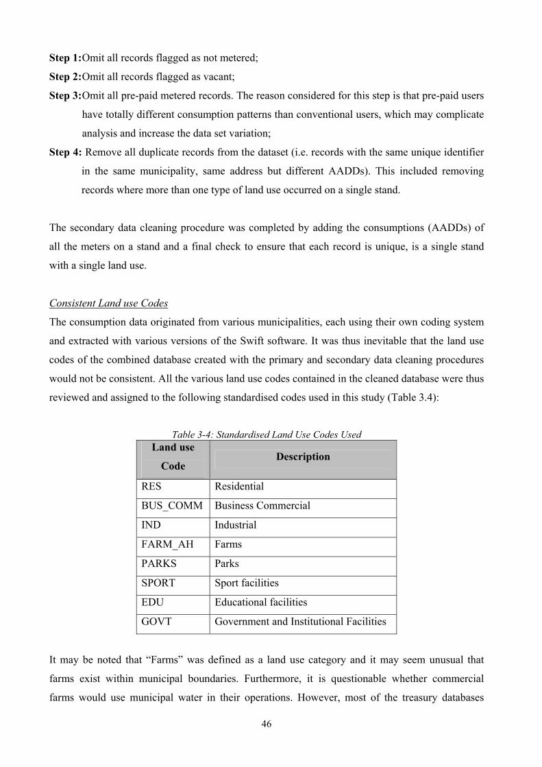
46
Step 1: Omit all records flagged as not metered;
Step 2: Omit all records flagged as vacant;
Step 3: Omit all pre-paid metered records. The reason considered for this step is that pre-paid users
have totally different consumption patterns than conventional users, which may complicate
analysis and increase the data set variation;
Step 4: Remove all duplicate records from the dataset (i.e. records with the same unique identifier
in the same municipality, same address but different AADDs). This included removing
records where more than one type of land use occurred on a single stand.
The secondary data cleaning procedure was completed by adding the consumptions (AADDs) of
all the meters on a stand and a final check to ensure that each record is unique, is a single stand
with a single land use.
Consistent Land use Codes
The consumption data originated from various municipalities, each using their own coding system
and extracted with various versions of the Swift software. It was thus inevitable that the land use
codes of the combined database created with the primary and secondary data cleaning procedures
would not be consistent. All the various land use codes contained in the cleaned database were thus
reviewed and assigned to the following standardised codes used in this study (Table 3.4):
Table 3-4: Standardised Land Use Codes Used Land use
Code Description
RES Residential
BUS_COMM Business Commercial
IND Industrial
FARM_AH Farms
PARKS Parks
SPORT Sport facilities
EDU Educational facilities
GOVT Government and Institutional Facilities
It may be noted that “Farms” was defined as a land use category and it may seem unusual that
farms exist within municipal boundaries. Furthermore, it is questionable whether commercial
farms would use municipal water in their operations. However, most of the treasury databases
47
contained “Farms” as a land use category. Judging by the stand sizes, most of these are actually
agricultural small holdings, although some small towns especially in the Western Cape, did have
significant sized farms within municipal boundaries. It was therefore decided to keep, as part of the
analysis, this land use category as a type of use in its own right.
Domestic Group Housing
This study differentiated between single residential stands (i.e. single dwelling per stand) and
domestic group housing. Domestic group housing is understood to be flats, townhouses, clusters
and duplexes. An attempt was made to create a specific land use category for domestic group
housing and to analyse water consumption patterns for this land use category. Group housing is a
residential land use type that is increasing in present day South Africa, especially in metropolitan
areas where space is limited and security is becoming an issue. It was anticipated that the water
demand patterns for group housing would differ significantly from the more conventional single
residential housing.
However, in extracting the consumption data from the municipal treasury systems it was noticed
that where stands were assigned as group housing, a single meter could be measuring the
consumption of the entire development (i.e. block(s) of flats) or a meter per unit could be
measuring consumption (e.g. A cluster development with a meter per unit). There was a field in
Swift that indicated the number of units attached to a meter. This information was extracted by
Swift from the treasury systems and used. The calculated consumption value had to be thus
divided with the number of units linked to the water meter for the group housing land use category.
However, in analysing the results of this calculation, it was evident by the large number of group
housing records, that either had extremely high or extremely low consumption levels, that the
possibility existed, that the information on the number of units contained in the treasury systems
might not always be very accurate. For this reason, it was considered prudent not to use the group
housing data for this study. Nevertheless, there is a possibility to use this data in another study, if
proper data cleaning and verification could be done, which was considered to fall outside the scope
of this study.
It is however, understood that it was very probable that some group housing were still included in
the final dataset that was analysed. This would be houses that were not identified as group housing
in the treasury data and thus included. It is expected, that typically this would be cluster type
houses or high security residential developments as these developments are mostly considered to
be single residential by municipalities with a single meter installed per house.

48
3.3 Data on Parameters Influencing Water Consumption Patterns 3.3.1 Data Collection Water demand patterns vary significantly from suburb to suburb, even in relatively cohesive areas
such as Gauteng (Stephenson and Turner, 1996). Various factors influence every user’s decision
on how much water he/she wants to use and when. Factors influencing water demand can be found
in the answers to questions such as “Does the user have a garden?”, “Is it a large garden?”, “Has it
been a dry summer?”, and “Can the user afford the water?”. However, to answer these questions
for millions of users is an impossible task. The design engineer therefore is faced with the problem
of estimating water demand and thus has to, in a sense, predict the user’s decision to use or not to
use water. Understanding the possible factors that may influence the user’s decision on how much
water they want to use has been a starting point of this study. The literature review undertaken as
part of this study (Chapter 2) indicated that the following factors influence municipal domestic
water demand patterns:
Stand area
Income level (stand value)
Climate
Water tariffs
In the literature review undertaken, very little information was presented as to the possible factors
influencing municipal non-domestic water demand patterns.
Data was collected for stand area, income level, climate and other socio-economic factors such as
level of unemployment, level of sanitation, household size, etc. At the start of this research, it was
anticipated that tariff data in the treasury data would be used for the evaluation of water price on
water demand. However, the tariff data extracted from the treasury databases was not as accurate
or available as was hoped. For some municipalities tariff data was available but with no
explanation of the coding system. For some other municipalities, codes were provided but the
database not populated. Some had no data on tariffs at all. Furthermore, the treasury data were
obtained in different time periods which would result in using 1998 tariffs for one data set and
comparing them with 2005 tariffs in another data set. It was therefore not deemed prudent to use
the tariff data that was available.
Table 3.5 indicates the sources of data on parameters influencing water demand.

49
Table 3-5: Data Sources for Parameters Influencing Water Demand Factor Source from where data was collected
Stand area Treasury data containing records of water consumption and user characteristics for individual connections such as stand area
Income Treasury data containing records of water consumption and user characteristics for individual connections such as stand value which was used as a proxy for income
Income
Socio-economic statistics per ward was obtained from the South African Municipal Demarcation Board. These statistics include level of unemployment, annual household income, level of sanitation, level of water service, household size
Climatic data (rainfall, average, maximum and minimum daily temperatures)
South African Weather Service
Mean Annual Precipitation Mean Annual Evaporation Surface Water Resources of South Africa by Midgley (1994)
It is important to observe that the stand value that was used in the analysis, was the sum of the
municipal valuations of the value of the stand itself and any improvements made that increased the
value of the stand. These values were all obtained from the treasury data.
3.3.2 Description of the Data
Climatic Data
The South African Weather Service (SAWS) was approached in June 2005 to supply climatic data
for this study. Daily precipitation, daily minimum and maximum temperatures, humidity and
evaporation data was requested for the period 01 January 1998 to 31 March 2005 for all the
appropriate locations studied in this investigation.
The SAWS supplied the climatic data summarised in Table 3.6 for the time period Jan 1998 to
March 2005. The SAWS could not supply data on humidity or evaporation since these
measurements are not taken any longer by the service. It was hoped at the beginning of the
research to have a higher resolution for climatic data, even as high as on suburb or group of
suburbs level in the metropolitan areas. However, there were quite a number of municipalities
where no data was available such as Oudtshoorn, Langeberg and Berg River, which cover several
towns. The data that was available was evaluated and verified and incorporated in the water
consumption database as discussed in the following section (3.3.3).
The WRC report by Midgley (1994) containing extensive information on MAP and MAE was
incorporated into the analysis to supplement the information supplied by SAWS. Appendix B
(supplied in electronic format only) contains tables indicating the locations and the MAP and MAE
stations used.

50
Table 3-6: Climatic Data Supplied by the SAWS Municipality Rainfall Station Name Temp Station Name
Alberton Ekurhuleni ALBERTON JOHANNESBURG INT WO Atteridgeville Tshwane PRETORIA EENDRACHT PRETORIA EENDRACHT Beaufort West BEAUFORT-WES BEAUFORT-WES Benoni Ekurhuleni BENONI - COUNTRY CLUB SPRINGS Berg River not available not available Blaauwberg (Cape Town) CAPE TOWN WO CAPE TOWN WO Boksburg Ekurhuleni BOKSBURG - BRANDWEER SPRINGS Brakpan Ekurhuleni SPRINGS SPRINGS Breede River ROBERTSON ROBERTSON Breede Valley WORCESTER-AWS WORCESTER-AWS Buffalo City Umzoniana not available Cape Agulhas not available not available Cederberg not available not available Centurion Tshwane PRETORIA EENDRACHT PRETORIA EENDRACHT Crocodile Tshwane PRETORIA EENDRACHT PRETORIA EENDRACHT Drakenstein MALMESBURY MALMESBURY Eastern JHB JOHANNESBURG INT WO JOHANNESBURG INT WO George GEORGE WO GEORGE WO Germiston Ekurhuleni ALBERTON JOHANNESBURG INT WO Helderberg STRAND STRAND Kempton Ekurhuleni BENONI - COUNTRY CLUB SPRINGS Langeberg not available not available Lethabong Ekurhuleni JOHANNESBURG SANDTON JOHANNESBURG INT WO Lethabong JHB JOHANNESBURG SANDTON JOHANNESBURG INT WO Mamelodi Tshwane PRETORIA EENDRACHT PRETORIA EENDRACHT Matzikama VREDENDAL VREDENDAL Midrand JHB JOHANNESBURG SANDTON JOHANNESBURG INT WO MosselBay not available not available Nigel Ekurhuleni SPRINGS SPRINGS Northern JHB JOHANNESBURG SANDTON JOHANNESBURG INT WO NPMSS Tshwane PRETORIA EENDRACHT PRETORIA EENDRACHT Odi Tshwane PRETORIA EENDRACHT PRETORIA EENDRACHT Oostenberg (Cape Town) CAPE TOWN WO CAPE TOWN WO Oudtshoorn not available not available Overstrand HERMANUS HERMANUS Plettenberg Bay PLETTENBERGBAAI PLETTENBERGBAAI Pretoria Tshwane PRETORIA EENDRACHT PRETORIA EENDRACHT Randfontein JOHANNESBURG INT WO JOHANNESBURG INT WO Saldanha LANGEBAANWEG WO LANGEBAANWEG WO Sedibeng VEREENIGING VEREENIGING Southern1 JHB JOHANNESBURG INT WO JOHANNESBURG INT WO Southern2 JHB JOHANNESBURG INT WO JOHANNESBURG INT WO Springs Ekurhuleni SPRINGS SPRINGS Stellenbosch SOMERSET WEST STRAND Swartland not available not available Temba Tshwane PRETORIA EENDRACHT PRETORIA EENDRACHT Theewaterskloof not available ROBERTSON Tygerberg (Cape Town) CAPE TOWN WO CAPE TOWN WO Western JHB JOHANNESBURG INT WO JOHANNESBURG INT WO
Socio-Economic Data

51
The South African Demarcation Board was approached to supply socio-economic statistics in
November 2005. The Board supplied all the data requested in electronic format. The following
statistics based on the Census 2001 data was supplied for every political ward in South Africa:
Ward identification
Number of employed persons
Number of unemployed persons
Number of economically active persons
Number of households living in a caravan or tent
Number of households living in flats or in blocks of flats
Number of households living in house or brick structures on a separate stand or yard
Number of households living in houses/flats/rooms in back yard
Number of households living in informal dwellings/shacks in back yard
Number of households living in informal dwellings/shacks NOT in backyard
Number of households living in private ships/boats
Number of households living in rooms/flatlets not in back yard but on shared property
Number of households living in town/cluster/semi-detached houses (simplex, duplex,
triplex)
Number of households living in traditional dwellings/huts/structures made of
traditional materials
Number of households for various intervals of household sizes
Number of Dwellings (houses) for various intervals of house sizes
Number of households with no income
Number of institutions where income is not applicable
Number of households for various intervals of annual income
Number of households with no access to piped potable water
Number of households with access to piped potable water to their dwelling
Number of households with access to piped potable water to their yard
Number of households with access to piped potable water more than 200 m from their
dwelling
Number of households with access to piped potable water less than 200 m from their
dwelling
Number of households with no sanitation
Number of households with bucket latrine sanitation
52
Number of households with chemical toilet sanitation
Number of households with flush sewerage sanitation
Number of households with flush septic tank sanitation
Number of households with pit latrine ventilated sanitation
Number of households with Pit latrine no ventilation sanitation
3.3.3 Data Verification and Linking to Water Consumption Data
Climatic Data
The SAWS provided the available climatic data (precipitation and minimum and maximum
temperatures)) for every day for the time period 01 January 1998 to 31 March 2005. The data was
provided in text format (‘.txt” files) and thus had to be incorporated in Microsoft Access format.
For both the rainfall and temperature datasets, there were a number of days on which
measurements were not taken or missing or estimated. The data was evaluated and if the impact of
the missing data was considered to be significant the dataset for the month was discarded. The
monthly averages were calculated for each available measurement station for both precipitation
and temperature. Where estimates or missing data were included in the calculated monthly
average, the calculated value was flagged as a possibly unreliable record.
The climatic data was linked to the water consumption database on the basis of municipality.
Section 3.2.2 discusses why a higher resolution such as town or suburb could not be used. To link
the climatic data to the water consumption database, the time period for the majority readings for a
municipality had to be determined. Table 3.1 gives the time period for the majority of readings per
municipality. For each municipality, the average annual rainfall and average annual maximum and
minimum temperature for the period of consumption measurement were determined from the data
of the closest climatic measurement station where available.
The published MAP and MAE values (Midgley et al.,1994) were linked to the water consumption
database by first establishing the most appropriate MAP and MAE stations for each town and
where possible suburb or group of suburbs in metropolitan areas. This was done by using the
longitude and latitude information of the climatic stations. The MAP and MAE values were
captured manually into the water consumption database by creating a town /suburb table with the
relevant corresponding MAP and MAE values and then linking the data automatically to the larger
water consumption database.

53
Socio-Economic Data
From the socio-economic data provided by the South African Demarcation Board (Section 3.2.2)
the following averages were calculated per political ward:
% Unemployment
% Formal Housing
Average Household size (weighted average)
Average House size (weighted average)
Average Income (weighted average)
% of dwellings with potable water house connection
% of dwellings with waterborne sanitation
To link the socio-economic data to the water consumption database was a complicated process.
The main problem being that the socio-economic data was made available by the South African
Demarcation Board on the basis of political wards. The water consumption data obtained from the
municipal treasury systems was based on suburbs. The wards thus had to be superimposed onto the
suburbs as accurately as possible. In other words, for each suburb, it had to be decided in which
political ward it fell. As the socio-economic database only had ward numbers and special place
names for some wards this process was not straightforward at all. Use was made of mapping
software provided by the South African Demarcation Board named SA Explorer. SA Explorer has
a GIS interface (Arcview) and enables the user to view the ward boundaries in relation to major
roads, rivers and places. The process of linking the socio-economic data to the water consumption
database was thus a manual process. For approximately 13% of the suburbs, it could not be
established in which ward they fell. This was mainly because there was limited information on
special place names in the wards which could be linked to a suburb or because the suburb fell into
two different wards. Another problem encountered with the socio-economic data being only
available on the political ward level was that in some wards, high income and low income suburbs
or areas had be grouped together in one ward. In such a case, one would not expect the water
demand to be homogenous. However, these cases were definitely in the minority.
It should also be noted that the socio-economic data was only linked for domestic consumers, as it
was considered that the socio-economic data such as income would have little or no influence on
non-domestic use.

54
4 METHODOLOGY
4.1 Data Filtering
The data cleaning and verification procedure created a single database including data on water
consumption and data on parameters that possibly affect water demand (climate and socio-
economic data). The database was spilt into 25 separate databases, each database representing a
land use type. There were 7 non-domestic user type databases and 18 domestic user type databases.
The 18 domestic user databases were created from the domestic data broken down into similar
stand areas (creating 8 databases) and similar stand values (creating 10 databases).. Each database
comprised some or all the following fields:
A unique identifier that can be linked back to the treasury data and address and other customer
and meter information;
Land use code;
Suburb Category that can be linked to a suburb;
Annual average daily demand (AADD) in kl/day;
Period of calculation for the AADD (dates);
Stand Area (m2);
Stand Value (R);
Geographic location of the stand (either “Coastal” or “Inland”) The geographic location was
given a numeric value namely Coastal = 1 and Inland = 2;
Development Level (either City/ Metro or small town/rural) (This field was only included for
the non-domestic users as it was expected that the development level may have a significant
influence on non-domestic use i.e. larger industries, educational facilities etc in the cities). The
development level was also assigned a numeric value, namely City/Metro = 1 and Rural/Small
town = 2;
Mean Annual Precipitation (mm) for the area where the stand is located;
Mean Annual Evaporation (mm) for the area where the stand is located;
Average Maximum Temperature for the water consumption measurement period (degree
Celsius);
Average Minimum Temperature for the water consumption measurement period (degree
Celsius);
Unique political ward ID as obtained from the South African Demarcation Board *;
Percentage of unemployed persons in the economically active population*;

55
Percentage of households with formal housing (not informal or traditional dwellings)*;
Average household size (no. of persons)*;
Average house size (no. of rooms)*;
Average household income*;
Percentage of houses with potable water house connection (i.e. not a stand pipe etc)*;
Percentage dwellings/houses with water-borne sanitation (i.e. flush toilets)*.
Note: *data only available on ward level and only included in the domestic databases as these
factors were not considered to have an impact on non-domestic use
The next step involved selecting only those stands that reasonably represent each land use
category. Filters were thus applied to the databases to exclude users with unrealistically low or
high stand areas and stand values. These values may not necessarily be wrong, but were omitted on
the basis that it is not practical to supply every possible type of consumer through the municipal
water distribution system. Table 4.1 summarises the criteria used for the data filters. The cut-off
points were decided by pragmatic consideration judging the data range in each case. From the
stand area and stand value ranges shown in Table 4.1, every effort was made to retain as many
records as was possible.
Table 4-1: Data Filters Applied to Water Consumption Data Land Use Category Stand area (m2) Stand Value (R)
Single residential >20 m2 and <= 4000 m2 >R20,000 and <=R10 million Business Commercial >20 m2 and <= 50 000 m2 >R20,000 and <=R100 million Industrial >20 m2 and <= 50 000 m2 >R20,000 and <=R100 million Farms >5000 m2 >R20,000 and <=R10 million Sport and Parks >500 m2 and <= 100 000 m2 >R20,000 and <=R20 million Education >100 m2 and <= 75 000 m2 >R20,000 and <=R20 million Government and Institutional >100 m2 and <= 50 000 m2 >R20,000 and <=R20 million
It may seem that the lower cut-off value for the stand value attribute is unreasonably low for all the
land use categories. However it has to be borne in mind that the data for the stand values originated
from treasury systems that may not have been updated for many years. Using a higher cut-off
value would have resulted in losing a large number of records. Table 4.2 below provides an
indication of the distribution of the number of domestic users for various stand value intervals. It is
clear that the majority of stands had values less than R500 000 in the treasury data. It seemed
therefore, that the majority of the data might have outdated or lower than expected stand values. It
could be argued that using the outdated stand values in combination with more up to date stand
values in the data analysis would only result in significant unexplained variation in the final
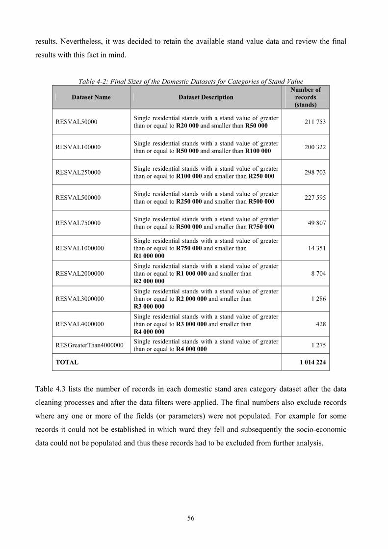
56
results. Nevertheless, it was decided to retain the available stand value data and review the final
results with this fact in mind.
Table 4-2: Final Sizes of the Domestic Datasets for Categories of Stand Value
Dataset Name Dataset Description Number of
records (stands)
RESVAL50000 Single residential stands with a stand value of greater than or equal to R20 000 and smaller than R50 000 211 753
RESVAL100000 Single residential stands with a stand value of greater than or equal to R50 000 and smaller than R100 000 200 322
RESVAL250000 Single residential stands with a stand value of greater than or equal to R100 000 and smaller than R250 000 298 703
RESVAL500000 Single residential stands with a stand value of greater than or equal to R250 000 and smaller than R500 000 227 595
RESVAL750000 Single residential stands with a stand value of greater than or equal to R500 000 and smaller than R750 000 49 807
RESVAL1000000 Single residential stands with a stand value of greater than or equal to R750 000 and smaller than R1 000 000
14 351
RESVAL2000000 Single residential stands with a stand value of greater than or equal to R1 000 000 and smaller than R2 000 000
8 704
RESVAL3000000 Single residential stands with a stand value of greater than or equal to R2 000 000 and smaller than R3 000 000
1 286
RESVAL4000000 Single residential stands with a stand value of greater than or equal to R3 000 000 and smaller than R4 000 000
428
RESGreaterThan4000000 Single residential stands with a stand value of greater than or equal to R4 000 000 1 275
TOTAL 1 014 224
Table 4.3 lists the number of records in each domestic stand area category dataset after the data
cleaning processes and after the data filters were applied. The final numbers also exclude records
where any one or more of the fields (or parameters) were not populated. For example for some
records it could not be established in which ward they fell and subsequently the socio-economic
data could not be populated and thus these records had to be excluded from further analysis.

57
Table 4-3: Final Sizes of the Domestic Datasets for Categories of Stand Area Dataset Name Dataset Description Number of
Records (stands)
RES500 Single residential stands with stand areas of greater than or equal to 20 m2 and smaller than 500 m2 433 104
RES750 Single residential stands with stand areas of greater than or equal to 500 m2 and smaller than 750 m2 112 443
RES1000 Single residential stands with stand areas of greater than or equal to 750 m2 and smaller than 1 000 m2 136 019
RES1500 Single residential stands with stand areas of greater than or equal to 1 000 m2 and smaller than 1 500 m2 184 497
RES2000 Single residential stands with stand areas of greater than or equal to 1 500 m2 and smaller than 2 000 m2 49 952
RES2500 Single residential stands with stand areas of greater than or equal to 2 000 m2 and smaller than 2 500 m2 17 506
RES3000 Single residential stands with stand areas of greater than or equal to 2 500 m2 and smaller than 3 000 m2 6 884
RES4000 Single residential stands with stand areas of greater than or equal to 3 000 m2 and smaller than 4 000 m2 6 168
TOTAL 946 573
Table 4.4 lists the number of records in each non-domestic dataset after the data cleaning processes
and after the data filters were applied:
Table 4-4: Final Sizes of the Non-Domestic Datasets.
Data Set Name Number of records
Business Commercial 24 810Education 1 447Farms 8 895Government & Institutions 8 259Industrial 8 000Parks 367Sport 68Total 51 846
The number of records in the Sport category was very small and it was expected that no statistical
significant results would be obtained for this category.
58
4.2 Data Analysis and Demand Estimation 4.2.1 Domestic Water Consumption – Assessment of the Existing Design Guidelines
The first step in the data analysis was a direct comparison of the domestic data with the “Red
Book” (CSIR, 2003) demand estimate guideline for domestic use. To do this comparison, it had to
be assumed that the climatic and socio-economic factors in a suburb were fairly homogenous. The
average stand area and the average AADD for a suburb were thus determined and these values
were plotted against the upper and lower limits given as a demand estimate guideline in the “Red
Book” (CSIR, 2003).
A single variable regression analysis was also done with ln(StandArea) specified as the
independent variable and ln(AADD) as the dependent variable using all the domestic data (i.e. not
categorising the data in datasets of different intervals for stand area). SPS statistical analysis
software was used to perform this regression analysis with 1 091 685 domestic records
countrywide.
The assessment of the Red Book design guidelines were further refined by categorising the data
(1 091 685 records) in two categories for geographic location namely coastal or inland. A single
variable regression analysis was performed with stand area specified as the independent variable
for each category. The definition of ‘coastal’ used was a town or area directly adjacent to the sea.
For example the geographic location of Lamberts Bay (0 km from the coast) would be “coastal”
and Vredendal (approximately 50 km from the coast) would be “inland”.
4.2.2 Assessment of Factors Influencing Domestic Water Consumption
The next step was to also perform a step-wise multiple variable regression analysis for each of the
domestic stand area datasets with ln(AADD) specified as the dependent variable to determine
which factors correlates best with domestic consumption. A stepwise regression for more than one
independent variable will always select the variable that correlates best with the dependent variable
first and then the next best correlation and so forth. Thus multiple variable models were obtained
for various stand area and stand value categories of domestic demand. This provided models of the
combined effect of the parameters influencing domestic water demand. The regression statistics for
each of the regressions are discussed in detail in Chapter 5.

59
The stepwise regression models informed the decision as to which two variables influence water
demand the most in each land use category. In most cases, it was the ln(StandValue) and the
ln(StandArea). Thus for these two parameters, single variable regression models were calculated
with 95% confidence intervals for each land use category. The single variable regression models
were further refined by distinguishing between the geographic location (e.g. inland or coastal).
Figure 4.1 portrays schematically the number of single variable regression models calculated for
domestic user categories. Thus for every domestic user category 4 single variable regression
models were created and with 95% confidence limits for the mean of the AADD. The regression
results of each of these models are discussed in detail in Chapter 5.
Domestic User Category GL?
Ln(AADD) =f (Ln(StandArea)
Ln(AADD) =f (Ln(StandValue)
Ln(AADD) =f (Ln(StandArea)
Ln(AADD) =f (Ln(StandValue)
CO
ASTA
LIN
LAN
D
GL = Geographic Location (Coastal or Inland)
Figure 4-1: Single Variable Regression Models for Domestic User Categories
4.2.3 Non-Domestic Water Consumption
The first step was to calculate frequency distributions and descriptive statistics for each of the
datasets to better understand the nature of each dataset. In the literature review undertaken with
this study very little previous work was found on water consumption estimation of non-domestic
users for municipal services design purposes. Therefore this step was considered necessary. The
frequency distributions were calculated for intervals of the natural logarithm of the demand
(AADD).
The next step was to perform a step-wise multiple variable regression analysis for each land use
dataset with ln(AADD) specified as the dependent variable. By doing a stepwise regression it
could be established which variables (or parameters) influences non-domestic water demand the

60
most and also obtain a model of the combined effect of the parameters influencing water demand.
The regression statistics for each of the regressions are discussed in detail in Chapter 5.
As was the case with the domestic analysis the stepwise regression models informed the decision
as to which two variables influences water demand the most in each land use category and
consequently single variable regression models with 95% confidence intervals were also calculated
with stand area and stand value specified as independent variables for each land use category. The
single variable regression models were further refined by distinguishing between the geographic
location (e.g. inland or coastal) and the development level (e.g. metro and city or small town rural).
Figure 4.2 portrays schematically the number of single variable regression models calculated for
non-domestic user categories . Thus for every non-domestic user category 8 single variable
regression models with 95% confidence limits for the mean of the AADD were calculated. The
regression results of each of these models are discussed in detail in Chapter 5.
Non Domestic User Category
GL?
Ln(AADD) =f (Ln(StandArea)
Ln(AADD) =f (Ln(StandValue)
Ln(AADD) =f (Ln(StandArea)
Ln(AADD) =f (Ln(StandValue)
CO
ASTA
LIN
LAN
D
DL?
GL?
Ln(AADD) =f (Ln(StandArea)
Ln(AADD) =f (Ln(StandValue)
Ln(AADD) =f (Ln(StandArea)
Ln(AADD) =f (Ln(StandValue)
MET
RO
/ CIT
YSM
ALL
TOW
N /R
UR
AL
CO
ASTA
LIN
LAN
D
GL = Geographic Location (Coastal or Inland)
DL = Development Level
(City/Metro or Small Town /rural)
Figure 4-2: Single Variable Regression Models for Non-Domestic User Categories
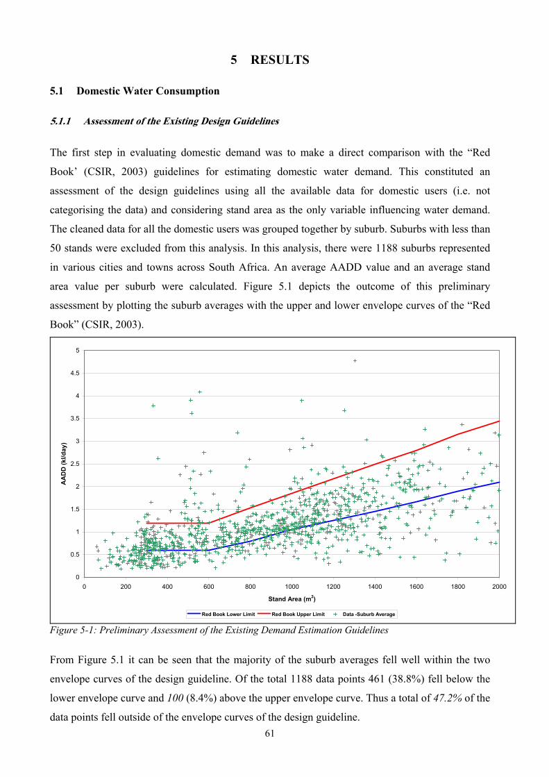
61
5 RESULTS
5.1 Domestic Water Consumption 5.1.1 Assessment of the Existing Design Guidelines
The first step in evaluating domestic demand was to make a direct comparison with the “Red
Book’ (CSIR, 2003) guidelines for estimating domestic water demand. This constituted an
assessment of the design guidelines using all the available data for domestic users (i.e. not
categorising the data) and considering stand area as the only variable influencing water demand.
The cleaned data for all the domestic users was grouped together by suburb. Suburbs with less than
50 stands were excluded from this analysis. In this analysis, there were 1188 suburbs represented
in various cities and towns across South Africa. An average AADD value and an average stand
area value per suburb were calculated. Figure 5.1 depicts the outcome of this preliminary
assessment by plotting the suburb averages with the upper and lower envelope curves of the “Red
Book” (CSIR, 2003).
0
0.5
1
1.5
2
2.5
3
3.5
4
4.5
5
0 200 400 600 800 1000 1200 1400 1600 1800 2000
Stand Area (m2)
AA
DD
(kl/d
ay)
Red Book Lower Limit Red Book Upper Limit Data -Suburb Average
Figure 5-1: Preliminary Assessment of the Existing Demand Estimation Guidelines
From Figure 5.1 it can be seen that the majority of the suburb averages fell well within the two
envelope curves of the design guideline. Of the total 1188 data points 461 (38.8%) fell below the
lower envelope curve and 100 (8.4%) above the upper envelope curve. Thus a total of 47.2% of the
data points fell outside of the envelope curves of the design guideline.

62
An analysis of the suburbs that fell outside the upper guideline curve was made and found that
57% of the data points represented suburbs with average stand areas smaller than 800 m2. The
suburbs that had consumption values above the upper guideline curve were mostly a combination
middle income smaller single residential developments such as Cason in Boksburg, Brixton and
Yeoville in Johannesburg and low income or township developments such as Orange Grove
(Johannesburg) and Ncala in Germiston. However, a number of high income high security
developments such as Kyalami Estates, Dainfern, Douglasdale and Sunning Hill in the northern
suburbs were also found among the suburbs with higher water consumptions. Approximately 23 of
the 100 suburbs, with greater water consumption than predicted by the “Red Book”, could be
classified as high income and typically high security developments.
The single variable regression analysis, that was done for all 1 091 685 domestic stands
countrywide, with stand area specified as the independent variable, resulted in the following
regression equation for the average of all stands with 95% confidence limits:
666977)4124.6(ln1016.9860.0)ln(297.0610.1)ln(2
7 StdAreaStdAreaAADD (5.1)
Where
StdArea = Stand Area in m2
AADD = Annual Average Daily Demand (kl/day)
The first part of the equation (before ±) describes the average water demand curve, and the second
part the 95% confidence interval. The regression model had an adjusted R square value (square of
the Pearson product moment correlation coefficient) of 0.218, which implied that 21.8% of the
variability in the data could be explained by this equation. An adjusted R square value of more
than 20% is considered good when predicting human behaviour as was the case with this study.
Numerous factors contribute to the variability in the data and given the large dataset, even greater
variation could be expected. The t-statistics for the regression coefficients indicated that they were
significantly different from zero. The detailed regression statistics are included in Appendix C
(supplied in electronic format only). A logarithmic regression model was used as this gave the best
fit to the data. Figure 5.2 below plots the regression equation against the Red Book design
guideline envelope curves for domestic water use. The guideline curves of the Red Book were
extrapolated up to stand areas of 4 000 m2 in order to make the comparison. This study had more
than 30 000 residential stands with stand areas greater than 2000 m2. The Red Book only gives the
guideline curves up to a stand area of 2 000 m2.

63
00.5
11.5
22.5
33.5
4
4.55
5.56
6.57
0 500 1000 1500 2000 2500 3000 3500 4000
Stand Area (m2)
AA
DD
(kl/d
ay)
Ln(AADD) = 0.297ln(StandArea) - 1.61
Design Guideline Upper Limit (CSIR, 2003)
Design Guideline Low er Limit (CSIR, 2003)
Figure 5-2: Single Variable Regression Model with Stand Area for All Domestic Data
It can be seen from Figure 5.2 that the regression model predicts AADD values within the range of
the guideline envelope curves up to stand areas of approximately 1 700 m2. The regression line lies
very close to the upper limit for stand areas smaller than 750 m2. In fact, the model predicts
slightly higher AADD values for stand areas between 500 m2 and 750 m2. For stand areas larger
than 1 700 m2 the model predicts much lower AADD values. This result corresponds with the
preliminary evaluation that was made by comparing the suburb averages with the “Red Book”
guideline, namely that the majority of the stands that exhibited higher consumption than what the
guideline predicted were smaller stands (stand areas less than 800 m2).
Figure 5.3 plots the regression equation with its 95% confidence limits. The 95% confidence limits
lie very close to the regression line, so much so that the difference can hardly be distinguished. The
95% confidence limits indicate the 95% probability that the average AADD of all stands will lie
within these lower and upper limits. The extremely large dataset is responsible for the fact that the
confidence intervals lie so close to the regression line.
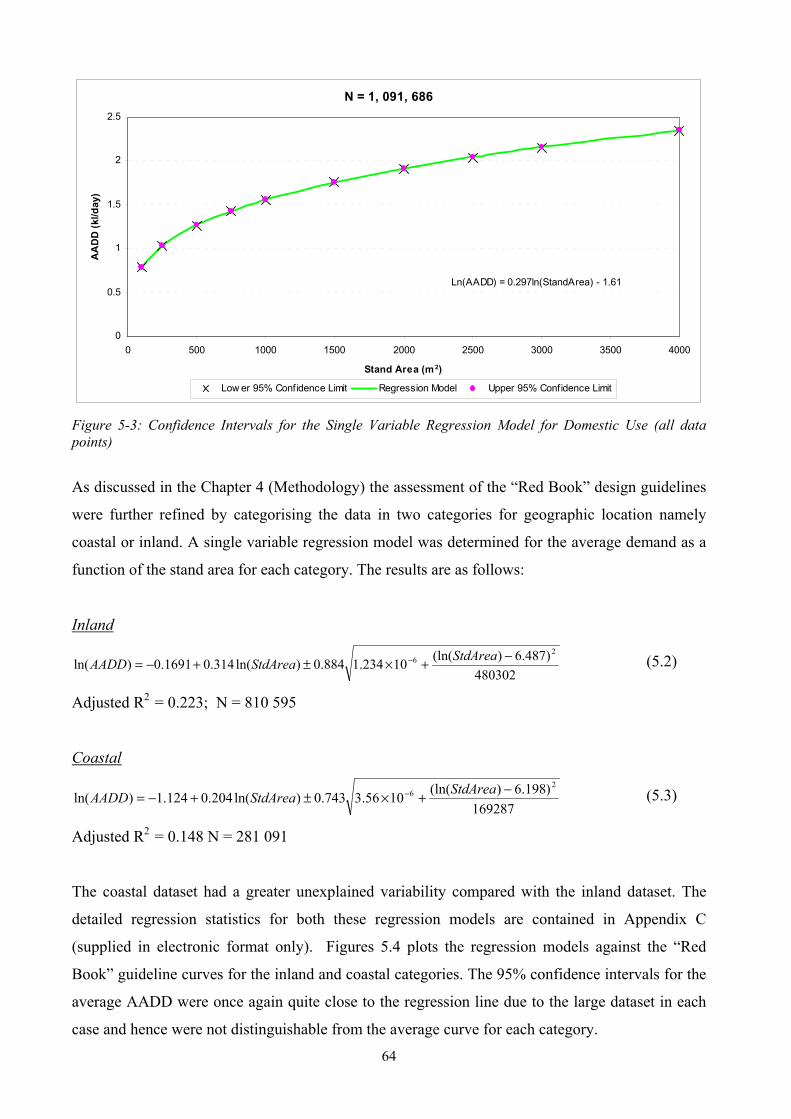
64
N = 1, 091, 686
0
0.5
1
1.5
2
2.5
0 500 1000 1500 2000 2500 3000 3500 4000
Stand Area (m2)
AA
DD
(kl/d
ay)
Low er 95% Confidence Limit Regression Model Upper 95% Confidence Limit
Ln(AADD) = 0.297ln(StandArea) - 1.61
Figure 5-3: Confidence Intervals for the Single Variable Regression Model for Domestic Use (all data points)
As discussed in the Chapter 4 (Methodology) the assessment of the “Red Book” design guidelines
were further refined by categorising the data in two categories for geographic location namely
coastal or inland. A single variable regression model was determined for the average demand as a
function of the stand area for each category. The results are as follows:
Inland
480302)487.6)(ln(10234.1884.0)ln(314.01691.0)ln(
26 StdAreaStdAreaAADD (5.2)
Adjusted R2 = 0.223; N = 810 595
Coastal
169287)198.6)(ln(1056.3743.0)ln(204.0124.1)ln(
26 StdAreaStdAreaAADD (5.3)
Adjusted R2 = 0.148 N = 281 091
The coastal dataset had a greater unexplained variability compared with the inland dataset. The
detailed regression statistics for both these regression models are contained in Appendix C
(supplied in electronic format only). Figures 5.4 plots the regression models against the “Red
Book” guideline curves for the inland and coastal categories. The 95% confidence intervals for the
average AADD were once again quite close to the regression line due to the large dataset in each
case and hence were not distinguishable from the average curve for each category.

65
0
0.5
1
1.5
2
2.5
3
3.5
4
0 500 1000 1500 2000 2500 3000 3500 4000
Stand Area (m2)
AA
DD
(kl/d
ay)
Inland: Ln(AADD) = 0.314ln(StandArea) - 1.691Adjusted R2 = 0.223
Coastal: Ln(AADD) = 0.204ln(StandArea) - 1.124Adjusted R2 = 0.148
Design Guideline Upper Limit
Design Guideline Low er Limit
Figure 5-4: Single Variable Regression Models for the Inland and Coastal Categories
From Figure 5.4, it can be seen that the regression models predict that domestic consumptions in
inland areas are generally higher than that of coastal areas. For stand areas less than 250 m2 the
geographic location makes no significant difference in the domestic water consumption. A possible
explanation for the seemingly higher consumption at inland location may be that quite a number of
the coastal towns studied constitute the typical holiday seaside town with a number of residences
only being occupied during holiday seasons. Not much gardening is done at these houses and thus
it could be expected that the water demand would be less when compared with an ‘inland’ house.
The regression model for coastal domestic consumption predicts that the average AADD will be
within the “Red Book” design guideline curves up to stand areas of approximately 1300 m2. For
stand areas larger than 1300 m2 the regression model indicates that the average domestic
consumption is likely to be less than the minimum “Red Book” curve. For inland domestic
consumption it seems that the model predicts the average AADD to fall well within the guideline
curves (excluding stand areas of about 500 m2 to 800 m2) up to stand areas of approximately 1800
m2. Thereafter the model predicts lower AADD values.

66
5.1.2 Assessment of Factors Influencing Domestic Water Consumption
All the domestic data was divided into 8 categories of similar stand area and also into 10 categories
of similar stand value, as discussed in detail in Chapter 4. On each of these 18 categories, a
stepwise multiple regression analysis was performed. Table 5.3 summarises the outcome of the
stepwise regression analyses on each category by listing the independent variables influencing
water consumption in each category by order of best correlation with AADD. The number of data
points in each analysis is also indicated and the adjusted R-square value of the each stepwise
regression model.
Table 5-1: Summary of the Outcome of the Stepwise Multi-Variable Regression Analyses on Domestic Categories
Category Description of the Category
Number of points
Number of
Variables
Independent Variables by order of Best Correlation
with Ln (AADD)
Cumulative Adjusted
R2
STAND AREA CATEGORIES Stand Area 0.053 Geographic Location 0.066 Ln (Stand Value) 0.079 Mean Annual Evaporation 0.082 Ave Min Temperature 0.087 % Unemployment 0.089 Ave Household Income 0.09 % Waterborne Sanitation 0.09 Ave Max Temperature 0.091 Mean Annual Precipitation 0.091 % Water Connection 0.091 Ave Household Size 0.091 % Formal Housing 0.091
RES500
Single residential stands with stand areas of greater than or equal to 20 m2 and smaller than 500 m2
433 104 14
Ave House Size 0.091 Ln(Stand Value) 0.037 Geographic Location 0.062 Ave Household Income 0.071 Mean Annual Precipitation 0.078 Ave House Size 0.085 Stand Area 0.088 % Water connection 0.09 Ave Max Temperature 0.094 Mean Annual Evaporation 0.097 Stand Value 0.099 % unemployed 0.101 Ave Min Temperature 0.101 Ave Household Size 0.102
RES750
Single residential stands with stand areas of greater than or equal to 500 m2 and smaller than 750 m2
112 443 14
Ln(Stand Area) 0.102 Ln(Stand Value) 0.067 Geographic Location 0.086 Ave Min Temperature 0.101 Mean Annual Evaporation 0.113 Mean Annual Precipitation 0.12 Ave Household Income 0.124
RES1000 Single residential stands with stand areas of greater than or equal to 750 m2 and smaller than 1 000 m2
136 019 14
Ave House Size 0.132

67
Category Description of the Category
Number of points
Number of
Variables
Independent Variables by order of Best Correlation
with Ln (AADD)
Cumulative Adjusted
R2
Stand Value 0.134 Stand Area 0.135 Ave Max Temperature 0.137 % water connection 0.139 % unemployed 0.14 % Formal Housing 0.14 % Waterborne Sanitation 0.141 Ln(Stand Value) 0.092 Ave Household Income 0.117 Ave House Size 0.139 Geographic Location 0.15 Mean Annual Precipitation 0.161 Stand Area 0.167 Ave Min Temperature 0.171 Mean Annual Evaporation 0.172 Stand Value 0.174 % Formal Housing 0.175 % Waterborne Sanitation 0.176 Ave Max Temperature 0.176 % unemployed 0.176 Ave Household size 0.177
RES1500
Single residential stands with stand areas of greater than or equal to 1 000 m2 and smaller than 1 500 m2
184 497 15
% house water connection 0.177 Ln(Stand Value) 0.105 Ave Household Income 0.132 Ave House Size 0.155 Geographic Location 0.163 Mean Annual Precipitation 0.169 % Formal Housing 0.171 Stand Value 0.173 Stand Area 0.173 Mean Annual Evaporation 0.174 Ln(Stand Area) 0.174
RES2000
Single residential stands with stand areas of greater than or equal to 1 500 m2 and smaller than 2 000 m2
49 952 11
% house water connection 0.174 Ln(Stand Value) 0.092 Geographic Location 0.125 Ave Household Income 0.136 Ave House Size 0.144 % Formal Housing 0.146 % unemployed 0.147 % water connection 0.148 Mean Annual Precipitation 0.149 Stand Value 0.15 Ave Household size 0.15
RES2500
Single residential stands with stand areas of greater than or equal to 2 000 m2 and smaller than 2 500 m2
17 506 11
Mean Annual Evaporation 0.15 Ln(Stand Value) 0.161 Geographic Location 0.187 Stand Area 0.194 Ave Household Income 0.199 Ave House Size 0.206 Mean Annual Precipitation 0.207 % Formal Housing 0.208
RES3000
Single residential stands with stand areas of greater than or equal to 2 500 m2 and smaller than 3 000 m2
6 884 8
% unemployed 0.208 Ln (Stand Value) 0.164 RES4000 Single residential stands
with stand areas of 6 168 8
Geographic Location 0.196

68
Category Description of the Category
Number of points
Number of
Variables
Independent Variables by order of Best Correlation
with Ln (AADD)
Cumulative Adjusted
R2
Stand Value 0.207 Mean Annual Evaporation 0.213 Ave Household Income 0.218 Ave Max Temperature 0.22 Mean Annual Precipitation 0.222
greater than or equal to 3 000 m2 and smaller than 4 000 m2
% Waterborne Sanitation 0.223 STAND VALUE CATEGORIES
Ln(Stand Value) 0.029 Ln(Stand Area) 0.041 Geographic Location 0.05 Stand Value 0.056 Ave Household Income 0.058 % Unemployed 0.062 Ave Min Temperature 0.063 Ave Max Temperature 0.067 Mean Annual Evaporation 0.07 % Waterborne Sanitation 0.071 % Formal Housing 0.072 Stand Area 0.073 Ave Household Size 0.073 Mean Annual Precipitation 0.073 % water connection 0.073
RESVAL50000
Single residential stands with a stand value of greater than or equal to R20 000 and smaller than R50 000
211 753 16
Ave House Size 0.073 Ln(Stand Area) 0.033 Geographic Location 0.049 Mean Annual Evaporation 0.055 Ave Min Temperature 0.058 Ln(Stand Value) 0.06 Ave Max Temperature 0.061 Ave Household Income 0.062 % Unemployed 0.065 % Formal Housing 0.066 Ave House Size 0.066 Stand Area 0.066 Mean Annual Precipitation 0.066 Stand Value 0.066
RESVAL100000
Single residential stands with a stand value of greater than or equal to R50 000 and smaller than R100 000
200 322 14
% water connection 0.066 Ln(Stand Area) 0.065 Geographic Location 0.089 Ave Household Income 0.099 Ave House Size 0.106 Stand Value 0.111 % water connection 0.114 % Unemployed 0.116 Mean Annual Precipitation 0.118 Ave Max Temperature 0.119 Ave Min Temperature 0.124 Mean Annual Evaporation 0.126 % Formal Housing 0.127 % Waterborne Sanitation 0.128 Ave Household size 0.128
RESVAL250000
Single residential stands with a stand value of greater than or equal to R100 000 and smaller than R250 000
298 703 15
Stand Area 0.128 Ln(Stand Area) 0.107 RESVAL500000 Single residential stands
with a stand value of 227 595 16
Ave Household Income 0.134

69
Category Description of the Category
Number of points
Number of
Variables
Independent Variables by order of Best Correlation
with Ln (AADD)
Cumulative Adjusted
R2
Ave House Size 0.152 Geographic Location 0.161 Stand Value 0.17 Mean Annual Precipitation 0.178 % water connection 0.181 Ave Household size 0.182 Ave Max Temperature 0.184 Ave Min Temperature 0.185 Mean Annual Evaporation 0.187 Stand Area 0.188 % Waterborne Sanitation 0.188 % Unemployed 0.188 % Formal Housing 0.188
greater than or equal to R250 000 and smaller than R500 000
Ln(Stand Value) 0.188 Ln(Stand Area) 0.102 Geographic Location 0.148 Ave Household Income 0.165 Ave House Size 0.179 Mean Annual Precipitation 0.185 Stand Area 0.189 Ln(Stand Value) 0.192 % Waterborne Sanitation 0.194 % Unemployed 0.197 Ave Max Temperature 0.198 % water connection 0.199 Mean Annual Evaporation 0.199
RESVAL750000
Single residential stands with a stand value of greater than or equal to R500 000 and smaller than R750 000
49 807 13
% Formal Housing 0.2 Geographic Location 0.087 Ln(Stand Area) 0.133 Mean Annual Precipitation 0.139 Ave Max Temperature 0.146 Ave Min Temperature 0.149 Ave Household Income 0.15 % Unemployed 0.159 % water connection 0.165 Ave House Size 0.166 Stand Area 0.167 Ln(Stand Value) 0.167 Mean Annual Evaporation 0.168
RESVAL1000000
Single residential stands with a stand value of greater than or equal to R750 000 and smaller than R1 000 000
14 351 13
% Formal Housing 0.168 Geographic Location 0.079 Ln(Stand Area) 0.118 Ave Min Temperature 0.141 % Unemployed 0.147 Ave Household Income 0.16 % water connection 0.169 Stand Value 0.175 Stand Area 0.18 Mean Annual Evaporation 0.184 Ave House Size 0.185 Ln(Stand Value) 0.185
RESVAL2000000
Single residential stands with a stand value of greater than or equal to R1 000 000 and smaller than R2 000 000
8 704 12
Mean Annual Precipitation 0.186 Ave Min Temperature 0.261 RESVAL3000000 Single residential stands
with a stand value of 1 286 9
% water connection 0.356
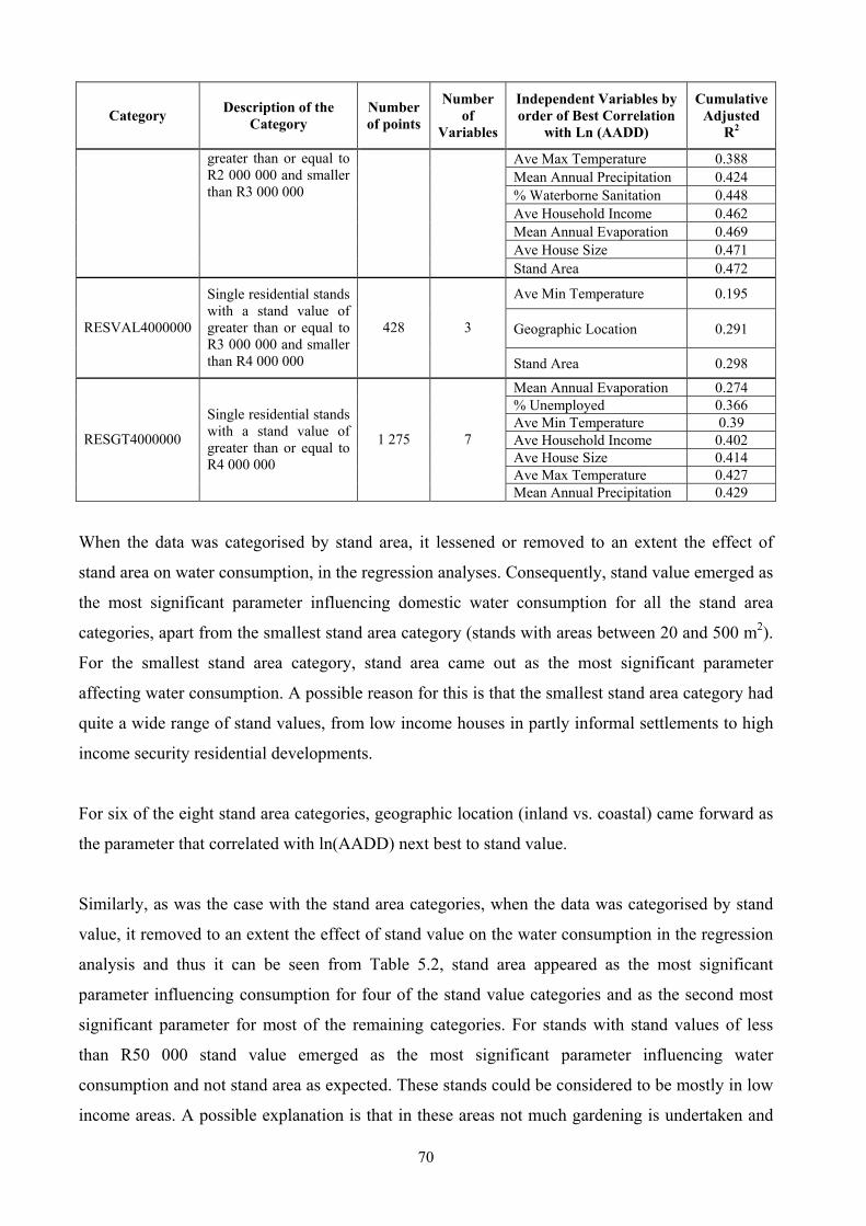
70
Category Description of the Category
Number of points
Number of
Variables
Independent Variables by order of Best Correlation
with Ln (AADD)
Cumulative Adjusted
R2
Ave Max Temperature 0.388 Mean Annual Precipitation 0.424 % Waterborne Sanitation 0.448 Ave Household Income 0.462 Mean Annual Evaporation 0.469 Ave House Size 0.471
greater than or equal to R2 000 000 and smaller than R3 000 000
Stand Area 0.472
Ave Min Temperature 0.195
Geographic Location 0.291 RESVAL4000000
Single residential stands with a stand value of greater than or equal to R3 000 000 and smaller than R4 000 000
428 3
Stand Area 0.298
Mean Annual Evaporation 0.274 % Unemployed 0.366 Ave Min Temperature 0.39 Ave Household Income 0.402 Ave House Size 0.414 Ave Max Temperature 0.427
RESGT4000000
Single residential stands with a stand value of greater than or equal to R4 000 000
1 275 7
Mean Annual Precipitation 0.429
When the data was categorised by stand area, it lessened or removed to an extent the effect of
stand area on water consumption, in the regression analyses. Consequently, stand value emerged as
the most significant parameter influencing domestic water consumption for all the stand area
categories, apart from the smallest stand area category (stands with areas between 20 and 500 m2).
For the smallest stand area category, stand area came out as the most significant parameter
affecting water consumption. A possible reason for this is that the smallest stand area category had
quite a wide range of stand values, from low income houses in partly informal settlements to high
income security residential developments.
For six of the eight stand area categories, geographic location (inland vs. coastal) came forward as
the parameter that correlated with ln(AADD) next best to stand value.
Similarly, as was the case with the stand area categories, when the data was categorised by stand
value, it removed to an extent the effect of stand value on the water consumption in the regression
analysis and thus it can be seen from Table 5.2, stand area appeared as the most significant
parameter influencing consumption for four of the stand value categories and as the second most
significant parameter for most of the remaining categories. For stands with stand values of less
than R50 000 stand value emerged as the most significant parameter influencing water
consumption and not stand area as expected. These stands could be considered to be mostly in low
income areas. A possible explanation is that in these areas not much gardening is undertaken and

71
hence stand area would not be expected to have to the most significant influence on water
consumption but rather stand value as a proxy for income.
The water consumption of stands that have values greater than R750 000 but smaller than R2
million was predicted by the multiple variable model to be mostly influenced by geographic
location (inland vs. coastal). While the water consumption of stands with values between R2
million and R4 million was dictated by the annual average minimum temperature. Mean Annual
Evaporation was indicated to be the most significant parameter influencing water consumption for
stands with values greater than R4 million.
Geographic location also emerged as a significant parameter influencing water demand for most
stand value categories.
The adjusted R-square values for most of the regression models appear to be quite low. However,
it should be kept in mind that human behaviour is being studied and an adjusted R-square value of
greater than 20% is considered a good fit when predicting human behaviour. Some R2 values are
still considerably smaller than 20%. This is especially true of the larger categories such as RES500
and RESVAL50000. It is true that more data points will have greater inherent variability and thus
lower adjusted R2 values. Once again, attention is drawn to the fact that the data for stand values
originated from different treasury systems covering different time periods over the last eight years
(1998 -2005). Furthermore, the stand value data might not have been updated regularly by
treasuries resulting in out of date stand values. This might result in, for example, a 1999 -2002
dataset still containing stand values for some records relating to say early nineties. This could
greatly contribute to the noted variability in the data. The regression models are all however,
considered to be statistically significant given the large dataset and the significant t- and F-
statistics.
It should also be noted that given the nature of the stand value data discussed above, this study
considered the stand values as a relative indication of the true values only. This stand value was
considered as a proxy indicator for income level defined as follows:
Table 5-2: Definition of Income Level Used in the Study Stand Value Range Income Level
R20 000 – R50 000 Very Low Income R50 000 – R100 000 Low Income R100 000 – R250 000 Low Middle Income R250 000 – R500 000 High Middle Income R500 000 – R750 000 High Income More than R750 000 Very High Income

72
Table 5.3 and Table 5.4 below summarise the first step regression equations (i.e. first step of the
regression with the independent variable that influenced AADD the most) that were obtained for
the stand area and stand value categories respectively. Appendix C (supplied in electronic format
only) can be consulted for the remaining models for each domestic category.
Table 5-3: Regression Results (First Step) of the Stepwise Multiple Variable Regression Analyses for Categories of Stand Area
Stand Area Category Regression Equation
>=20 m2 and < 500 m2 195.0001.0ln StdAreaAADD
>=500 m2 and < 750 m2 920.0)ln(099.0ln StdValueAADD
>=750 m2 and < 1000 m2 824.1)ln(181.0ln StdValueAADD
>=1000 m2 and < 1500 m2 595.2)ln(251.0ln StdValueAADD
>=1500 m2 and < 2000 m2 050.3)ln(295.0ln StdValueAADD
>=2000 m2 and < 2500 m2 788.2)ln(279.0ln StdValueAADD
>=2500 m2 and < 3000 m2 670.3)ln(348.0ln StdValueAADD
>=3000 m2 and < 4000 m2 453.3)ln(331.0ln StdValueAADD
Table 5-4: Regression Results (First Step) of the Stepwise Multiple Variable Regression Analyses for Categories of Stand Value
Stand Value Category Regression Equation
>=R20,000 and < R50,000 736.2)ln(266.0ln StdValueAADD
>=R50,000 and < R100,000 661.0)ln(133.0ln StdAreaAADD
>=R100,000 and < R250,000 910.0)ln(186.0ln StdAreaAADD
>=R250,000 and < R500,000 455.1)ln(286.0ln StdAreaAADD
>=R500,000 and < R750,000 159.1)ln(266.0ln StdAreaAADD
>=R750,000 and < R1,000,000 398.1)(427.0ln GLAADD
>=R1,000,000 and < R2,000,000 534.1)(446.0ln GLAADD
>=R2,000,000 and < R3,000,000 890.2)(172.0ln MinTempAADD
>=R3,000,000 and < R4,000,000 986.2)(123.0ln MinTempAADD
>=R4,000,000 336.3)(0027.0ln MAEAADD
Where: StdValue = Stand Value in R StdArea = Stand Area in m2 GL = Geographic Location where Inland = 2 and Coastal = 1 MinTemp =Annual Average Minimum Daily Temperature in degree Celsius MAE =Mean Annual Evaporation in mm
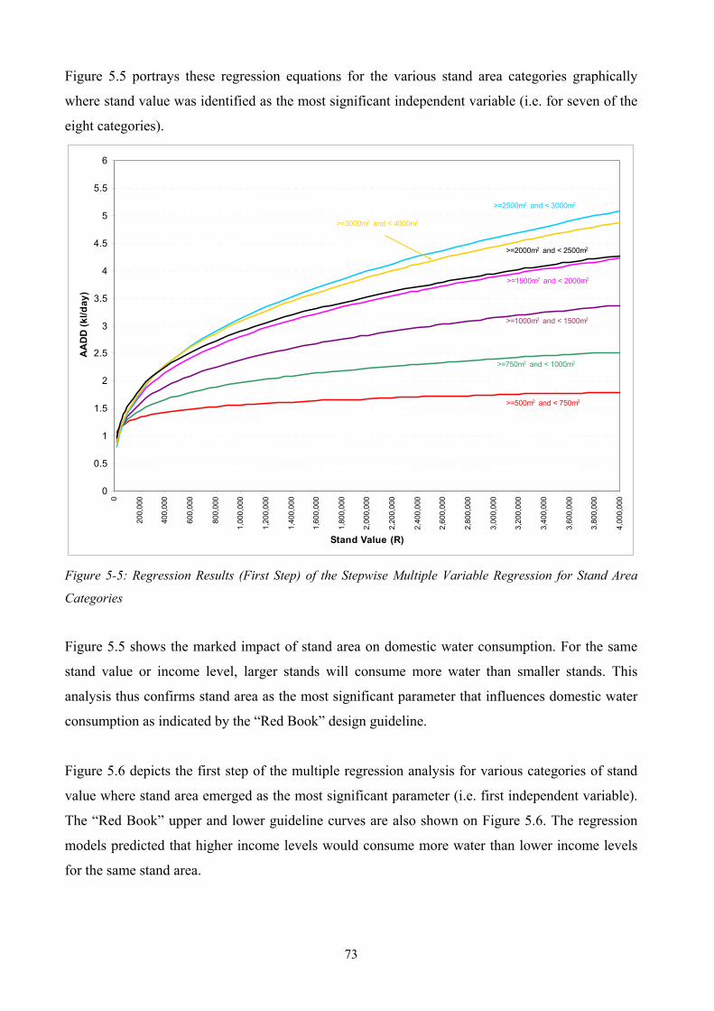
73
Figure 5.5 portrays these regression equations for the various stand area categories graphically
where stand value was identified as the most significant independent variable (i.e. for seven of the
eight categories).
0
0.5
1
1.5
2
2.5
3
3.5
4
4.5
5
5.5
6
0
200,
000
400,
000
600,
000
800,
000
1,00
0,00
0
1,20
0,00
0
1,40
0,00
0
1,60
0,00
0
1,80
0,00
0
2,00
0,00
0
2,20
0,00
0
2,40
0,00
0
2,60
0,00
0
2,80
0,00
0
3,00
0,00
0
3,20
0,00
0
3,40
0,00
0
3,60
0,00
0
3,80
0,00
0
4,00
0,00
0
Stand Value (R)
AA
DD
(kl/d
ay)
>=500m2 and < 750m2
>=750m2 and < 1000m2
>=1000m2 and < 1500m2
>=1500m2 and < 2000m2
>=2000m2 and < 2500m2
>=2500m2 and < 3000m2
>=3000m2 and < 4000m2
Figure 5-5: Regression Results (First Step) of the Stepwise Multiple Variable Regression for Stand Area
Categories
Figure 5.5 shows the marked impact of stand area on domestic water consumption. For the same
stand value or income level, larger stands will consume more water than smaller stands. This
analysis thus confirms stand area as the most significant parameter that influences domestic water
consumption as indicated by the “Red Book” design guideline.
Figure 5.6 depicts the first step of the multiple regression analysis for various categories of stand
value where stand area emerged as the most significant parameter (i.e. first independent variable).
The “Red Book” upper and lower guideline curves are also shown on Figure 5.6. The regression
models predicted that higher income levels would consume more water than lower income levels
for the same stand area.
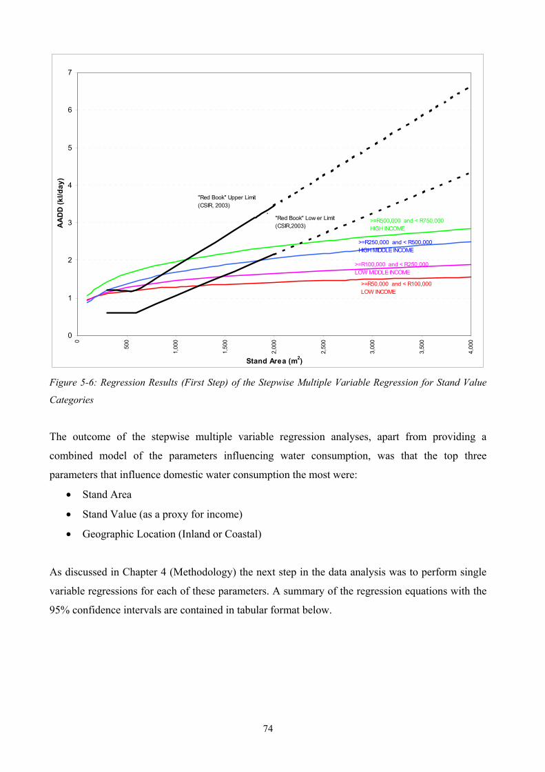
74
0
1
2
3
4
5
6
70
500
1,00
0
1,50
0
2,00
0
2,50
0
3,00
0
3,50
0
4,00
0
Stand Area (m2)
AA
DD
(kl/d
ay)
"Red Book" Upper Limit(CSIR, 2003)
"Red Book" Low er Limit(CSIR,2003)
>=R50,000 and < R100,000LOW INCOME
>=R100,000 and < R250,000LOW MIDDLE INCOME
>=R250,000 and < R500,000HIGH MIDDLE INCOME
>=R500,000 and < R750,000HIGH INCOME
`
Figure 5-6: Regression Results (First Step) of the Stepwise Multiple Variable Regression for Stand Value
Categories
The outcome of the stepwise multiple variable regression analyses, apart from providing a
combined model of the parameters influencing water consumption, was that the top three
parameters that influence domestic water consumption the most were:
Stand Area
Stand Value (as a proxy for income)
Geographic Location (Inland or Coastal)
As discussed in Chapter 4 (Methodology) the next step in the data analysis was to perform single
variable regressions for each of these parameters. A summary of the regression equations with the
95% confidence intervals are contained in tabular format below.

75
Tabl
e 5-
5: S
ingl
e Va
riab
le R
egre
ssio
n Re
sults
for D
omes
tic C
ateg
orie
s
Cat
egor
y G
eogr
aphi
c L
ocat
ion
Inde
pend
ent
Var
iabl
e E
quat
ion
N
Adj
uste
d R
2
Stan
d A
rea
2470
774
65
ln10
382
40
703
1ln
317
0ln
26
).
StdA
rea
(.
.(S
tdAr
ea)
.(A
ADD
)
333
880
0.04
1 In
land
Stan
d V
alue
15
6256
965
.10
ln10
381
70
505
.1ln
148
0ln
26
)St
dVal
ue(
.(S
tdVa
lue)
.(A
ADD
)
333
880
0.05
6
Stan
d A
rea
2668
363
45
ln10
9.660
70
899
.0ln
16.0ln
26
).
StdA
rea
(.
(Std
Area
)(A
ADD
)
145
019
0.04
7
RES
500
Coa
stal
Stan
d V
alue
86
141
216
.11
ln10
9.661
20
798
.0ln
072
0ln
26
)St
dVal
ue(
.(S
tdVa
lue)
.(A
ADD
)
145
019
0.03
Stan
d A
rea
1294
422
.6ln
102.1
829
054
7.2
ln43
60
ln2
5)
StdA
rea
(.
(Std
Area
).
(AAD
D)
86
291
0.
016
Inla
nd
Stan
d V
alue
41
605
791
.11
ln10
2.177
00
531
.1ln
153
0ln
25
)St
dVal
ue(
.(S
tdVa
lue)
.(A
ADD
)
80 4
73
0.07
3
Stan
d A
rea
755
425
.6ln
107.1
713
054
9.1
ln26
90
ln2
5)
StdA
rea
(.
(Std
Area
).
(AAD
D)
58
088
0.
07
RES
750
Coa
stal
Stan
d V
alue
36
686
137
.12
ln10
8.169
80
904
.0ln
089
0ln
25
)St
dVal
ue(
.(S
tdVa
lue)
.(A
ADD
)
56 3
54
0.03
9
Stan
d A
rea
977
805
.6ln
102.8
813
066
7.2
ln45
30
ln2
6)
StdA
rea
(.
(Std
Area
).
(AAD
D)
12
2 18
1 0.
01
Inla
nd
Stan
d V
alue
38
120
268
.12
ln10
2.877
6.0
402
.2ln
230
0ln
26
)St
dVal
ue(
(Std
Valu
e).
(AAD
D)
12
2 18
1 0.
095
Stan
d A
rea
285
77.6ln
108.2
786
053
3.1
ln26
90
ln2
5)
StdA
rea
(.
(Std
Area
).
(AAD
D)
35
667
0.
03
RES
1000
Coa
stal
Stan
d V
alue
19
510
509
.12
ln10
8.275
7.0
546
.1ln
147
0ln
25
)St
dVal
ue(
(Std
Valu
e).
(AAD
D)
35
667
0.
073
Stan
dAre
a 28
0206
7.7
ln10
7.586
40
399
.2ln
418
0ln
26
)St
dAre
a(
.(S
tdAr
ea)
.(A
ADD
)
175
128
0.01
4 R
ES15
00
Inla
nd
Stan
d V
alue
47
985
481
.12
ln10
7.581
7.0
090
.3ln
292
0ln
26
)St
dVal
ue(
(Std
Valu
e).
(AAD
D)
17
5 12
8 0.
118
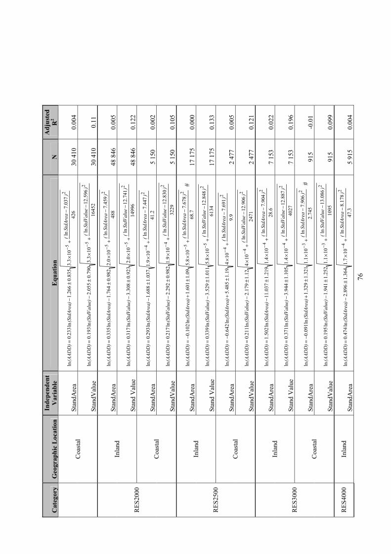
76
Cat
egor
y G
eogr
aphi
c L
ocat
ion
Inde
pend
ent
Var
iabl
e E
quat
ion
N
Adj
uste
d R
2
Stan
dAre
a 42
603
7.7
ln10
3.383
5.0
266
.1ln
233
0ln
25
)St
dAre
a(
(Std
Area
).
(AAD
D)
30
410
0.
004
Coa
stal
Stan
dVal
ue
1645
259
6.
12ln
103.3
790
.005
5.2
ln19
3.0
ln2
5)
StdV
alue
((S
tdVa
lue)
(AAD
D)
30
410
0.
11
Stan
dAre
a 48
845
9.7
ln10
0.298
2.0
764
.1ln
335
0ln
25
)St
dAre
a(
(Std
Area
).
(AAD
D)
48
846
0.
005
Inla
nd
Stan
d V
alue
14
996
741
.12
ln10
0.292
3.0
308
.3ln
317
0ln
25
)St
dVal
ue(
(Std
Valu
e).
(AAD
D)
48
846
0.
122
Stan
dAre
a 2.
4144
7.7
ln10
9.103
7.1
688
.1ln
293
0ln
24
)St
dAre
a(
(Std
Area
).
(AAD
D)
5
150
0.00
2
RES
2000
Coa
stal
Stan
dVal
ue
3229
830
.12
ln10
9.198
2.0
292
.2ln
217
0ln
24
)St
dVal
ue(
(Std
Valu
e).
(AAD
D)
5
150
0.10
5
Stan
dAre
a 7.
6867
8.7
ln10
8.509.1
601
.1ln
102
.0ln
25
)St
dAre
a(
(Std
Area
)(A
ADD
) #
17
175
0.
000
Inla
nd
Stan
d V
alue
61
3484
8.
12ln
108.5
011
.152
9.3
ln33
90
ln2
5)
StdV
alue
((S
tdVa
lue)
.(A
ADD
)
17 1
75
0.13
3
Stan
dAre
a 9.9
691
.7ln
104
19.148
5.5
ln64
2.0
ln2
4)
StdA
rea
((S
tdAr
ea)
(AAD
D)
2
477
0.00
5
RES
2500
Coa
stal
Stan
dVal
ue
2471
906
.12
ln10
412.1
179
.2ln
211
0ln
24
)St
dVal
ue(
(Std
Valu
e).
(AAD
D)
2
477
0.12
1
Stan
dAre
a 6.
2890
4.7
ln10
4.121
9.1
037
.11
ln50
2.1
ln2
4)
StdA
rea
((S
tdAr
ea)
(AAD
D)
7
153
0.02
2 In
land
Stan
d V
alue
40
2788
7.
12ln
104.1
105
.194
4.3
ln37
1.0
ln2
4)
StdV
alue
((S
tdVa
lue)
(AAD
D)
7
153
0.19
6
Stan
dAre
a 74
5.2
906
.7ln
101.1
321
.132
9.1
ln09
1.0
ln2
3)
StdA
rea
((S
tdAr
ea)
(AAD
D)
#
915
-0.0
1
RES
3000
Coa
stal
Stan
dVal
ue
1095
086
.13
ln10
1.125
2.1
941
.1ln
195
.0ln
23
)St
dVal
ue(
(Std
Valu
e)(A
ADD
)
915
0.09
9
RES
4000
In
land
St
andA
rea
3.47
178
.8ln
107.1
364
.189
6.2
ln47
4.0
ln2
4)
StdA
rea
((S
tdAr
ea)
(AAD
D)
5
915
0.00
4

77
Cat
egor
y G
eogr
aphi
c L
ocat
ion
Inde
pend
ent
Var
iabl
e E
quat
ion
N
Adj
uste
d R
2
Stan
d V
alue
31
1128
6.
13ln
107.1
266
.184
2.3
ln36
3.0
ln2
4)
StdV
alue
((S
tdVa
lue)
(AAD
D)
5
915
0.14
2
Stan
dAre
a 9
150
.8ln
109.8
462
.106.0
ln04
6.0
ln2
4)
StdA
rea
((S
tdAr
ea)
(AAD
D)
#
1 12
7 -0
.001
C
oast
al
Stan
dVal
ue
2811
765
.12
ln10
9.835
8.1
802
.1ln
175
.0ln
24
)St
dVal
ue(
(Std
Valu
e)(A
ADD
)
1 12
7 0.
137
Stan
d V
alue
Cat
egor
ies
Cat
egor
y G
eogr
aphi
c L
ocat
ion
Inde
pend
ent
Var
iabl
e E
quat
ion
N
Adj
uste
d R
2
Stan
dAre
a 22
414
712
.5ln
108.5
829
.059
8.0
ln11.0
ln2
6)
StdA
rea
((S
tdAr
ea)
(AAD
D)
17
1 57
8 0.
009
Inla
nd
Stan
d V
alue
18
561
276
.10
ln10
7.478
8.0
895
.2ln
283
.0ln
26
)St
dVal
ue(
(Std
Valu
e)(A
ADD
)
211
842
0.04
1
Stan
dAre
a 19
480
678
.5ln
108.1
619
.056
5.0
ln09
2.0
ln2
5)
StdA
rea
((S
tdAr
ea)
(AAD
D)
56
049
0.
028
RES
V50
000
Coa
stal
Stan
dVal
ue
3589
418
.10
ln10
7.163
3.0
645
.1ln
154
.0ln
25
)St
dVal
ue(
(Std
Valu
e)(A
ADD
)
59 7
84
0.01
3
Stan
dAre
a 36
382
938
.5ln
108.6
806
.052
7.0
ln11
5.0
ln2
6)
StdA
rea
((S
tdAr
ea)
(AAD
D)
14
6 42
4 0.
019
Inla
nd
Stan
d V
alue
57
3315
2.
11ln
108.6
809
.083.1
ln17
8.0
ln2
6)
StdV
alue
((S
tdVa
lue)
(AAD
D)
14
7 55
3 0.
007
Stan
dAre
a 28
561
769
.5ln
105.1
623
.055
2.0
ln10
1.0
ln2
5)
StdA
rea
((S
tdAr
ea)
(AAD
D)
66
168
0.
042
RES
V10
0000
Coa
stal
Stan
dVal
ue
2578
152
.11
ln10
54.1
655
.033
6.1
ln12
4.0
ln2 )
StdV
alue
((S
tdVa
lue)
(AAD
D)
70
281
0.
005
RES
V25
0000
In
land
St
andA
rea
6997
369
8.6
ln10
0.480
9.0
632
.0ln
148
.0ln
26
)St
dAre
a(
(Std
Area
)(A
ADD
)
252
741
0.03
4
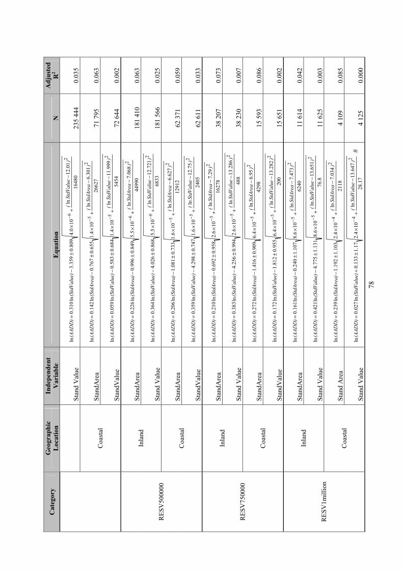
78
Cat
egor
y G
eogr
aphi
c L
ocat
ion
Inde
pend
ent
Var
iabl
e E
quat
ion
N
Adj
uste
d R
2
Stan
d V
alue
16
480
01.12
ln10
0.480
9.0
359
.3ln
310
.0ln
26
)St
dVal
ue(
(Std
Valu
e)(A
ADD
)
235
444
0.03
5
Stan
dAre
a 26
627
301
.6ln
104.1
655
.076
7.0
ln14
2.0
ln2
5)
StdA
rea
((S
tdAr
ea)
(AAD
D)
71
795
0.
063
Coa
stal
Stan
dVal
ue
5454
999
.11
ln10
4.168
4.0
583
.0ln
059
.0ln
25
)St
dVal
ue(
(Std
Valu
e)(A
ADD
)
72 6
44
0.00
2
Stan
dAre
a 44
990
068
.7ln
105.5
849
.099
6.0
ln22
6.0
ln2
6)
StdA
rea
((S
tdAr
ea)
(AAD
D)
18
1 41
0 0.
063
Inla
nd
Stan
d V
alue
68
3372
1.
12ln
105.5
868
.002
6.4
ln36
4.0
ln2
6)
StdV
alue
((S
tdVa
lue)
(AAD
D)
18
1 56
6 0.
025
Stan
dAre
a 12
912
627
.6ln
106.1
733
.008
1.1
ln20
6.0
ln2
5)
StdA
rea
((S
tdAr
ea)
(AAD
D)
62
371
0.
059
RES
V50
0000
Coa
stal
Stan
dVal
ue
2405
75.12
ln10
6.174
7.0
298
.4ln
359
.0ln
25
)St
dVal
ue(
(Std
Valu
e)(A
ADD
)
62 6
11
0.03
3
Stan
dAre
a 16
278
29.7ln
106.2
958
.069
2.0
ln21
0.0
ln2
5)
StdA
rea
((S
tdAr
ea)
(AAD
D)
38
207
0.
073
Inla
nd
Stan
d V
alue
48
828
6.
13ln
106.2
994
.025
6.4
ln38
3.0
ln2
5)
StdV
alue
((S
tdVa
lue)
(AAD
D)
38
230
0.
007
Stan
dAre
a 42
9895.6
ln10
4.690
9.0
416
.1ln
272
.0ln
25
)St
dAre
a(
(Std
Area
)(A
ADD
)
15 5
93
0.08
6
RES
V75
0000
Coa
stal
Stan
dVal
ue
200
282
.13
ln10
4.695
5.0
812
.1ln
172
.0ln
25
)St
dVal
ue(
(Std
Valu
e)(A
ADD
)
15 6
51
0.00
2
Stan
dAre
a 62
4047
3.7
ln10
6.810
7.1
240
.0ln
161
.0ln
25
)St
dAre
a(
(Std
Area
)(A
ADD
)
11 6
14
0.04
2 In
land
Stan
d V
alue
8.
7665
1.
13ln
106.8
131
.177
5.4
ln42
1.0
ln2
5)
StdV
alue
((S
tdVa
lue)
(AAD
D)
11
625
0.
003
Stan
d A
rea
2118
034
.7ln
104.2
103
.119
2.1
ln23
9.0
ln2
4)
StdA
rea
((S
tdAr
ea)
(AAD
D)
4
109
0.08
5
RES
V1m
illio
n
Coa
stal
Stan
d V
alue
17.
2864
7.
13ln
104.2
17.113
3.0
ln02
7.0
ln2
4)
StdV
alue
((S
tdVa
lue)
(AAD
D)
#
4 12
5 0.
000

79
Cat
egor
y G
eogr
aphi
c L
ocat
ion
Inde
pend
ent
Var
iabl
e E
quat
ion
N
Adj
uste
d R
2
Stan
d A
rea
5343
667
.7ln
105.1
325
.131
5.0
ln09
9.0
ln2
4)
StdA
rea
((S
tdAr
ea)
(AAD
D)
6
685
0.01
7 In
land
Stan
d V
alue
4.
224
039
.14
ln10
5.133
5.1
684
.1ln
196
.0ln
24
)St
dVal
ue(
(Std
Valu
e)(A
ADD
)
6 70
2 0.
003
Stan
dAre
a 21
7117
4.7
ln10
5.327.1
146
.1ln
249
.0ln
24
)St
dAre
a(
(Std
Area
)(A
ADD
)
2 85
5 0.
101
RES
V2m
illio
n
Coa
stal
Stan
dVal
ue
2.10
306
8.
14ln
105.3
356
.133
0.6
ln49
6.0
ln2
4)
StdV
alue
((S
tdVa
lue)
(AAD
D)
2
888
0.01
8
Stan
d A
rea
3.74
858
8.8
ln10
2.118
5.2
97.3ln
331
.0ln
23
)St
dAre
a(
(Std
Area
)(A
ADD
)
856
0.07
In
land
Stan
d V
alue
64.
1471
3.
14ln
102.1
189
.219.
35ln
316
.2ln
23
)St
dVal
ue(
(Std
Valu
e)(A
ADD
)
866
0.06
7
Stan
dAre
a 22
5427
8.8
ln10
3.171
3.1
654
.1ln
139
.0ln
23
)St
dAre
a(
(Std
Area
)(A
ADD
)
771
0.06
8
RES
V3m
illio
n
Coa
stal
Stan
d V
alue
13.
1372
1.
14ln
103.1
717
.112.
27ln
808
.1ln
23
)St
dVal
ue(
(Std
Valu
e)(A
ADD
)
777
0.06
6
Stan
d A
rea
63.27
256
8.8
ln10
6.312
1.2
455
.2ln
054
.0ln
23
)St
dAre
a(
(Std
Area
)(A
ADD
) #
28
1 -0
.001
In
land
Stan
d V
alue
09.2
03.15
ln10
5.309
5.2
701
.25
ln84
3.1
ln2
3)
StdV
alue
((S
tdVa
lue)
(AAD
D)
# 28
2 0.
018
Stan
d A
rea
4.38
799
2.7
ln10
4.301
7.2
027
.0ln
109
.0ln
23
)St
dAre
a(
(Std
Area
)(A
ADD
) #
29
6 0.
011
RES
V4m
illio
n
Coa
stal
Stan
d V
alue
18.2
045
.15
ln10
3.303
3.2
926
.16
ln06
5.1
ln2
3)
StdV
alue
((S
tdVa
lue)
(AAD
D)
# 30
2 0.
004
Stan
d A
rea
2.98
634
7.9
ln10
3.113
8.3
327
.1ln
070
.0ln
23
)St
dAre
a(
(Std
Area
)(A
ADD
) #
78
9 0.
001
RES
VG
T4m
illio
n In
land
Stan
d V
alue
7.
217
945
.15
ln10
2.113
6.3
926
.7ln
375
.0ln
23
)St
dVal
ue(
(Std
Valu
e)(A
ADD
)
805
0.01
3

80
Cat
egor
y G
eogr
aphi
c L
ocat
ion
Inde
pend
ent
Var
iabl
e E
quat
ion
N
Adj
uste
d R
2
Stan
d A
rea
1692
321
.9ln
103.9
603
.239
4.1
ln07
5.0
ln2
4)
StdA
rea
((S
tdAr
ea)
(AAD
D)
1
074
0.00
4 C
oast
al
Stan
d V
alue
1.
586
161
.16
ln10
3.962
6.2
883
.3ln
197
.0ln
24
)St
dVal
ue(
(Std
Valu
e)(A
ADD
)
1 07
9 0.
011
# Eq
uatio
n co
effic
ient
s do
not d
iffer
sign
ifica
ntly
from
zero
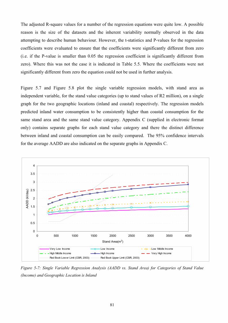
81
The adjusted R-square values for a number of the regression equations were quite low. A possible
reason is the size of the datasets and the inherent variability normally observed in the data
attempting to describe human behaviour. However, the t-statistics and P-values for the regression
coefficients were evaluated to ensure that the coefficients were significantly different from zero
(i.e. if the P-value is smaller than 0.05 the regression coefficient is significantly different from
zero). Where this was not the case it is indicated in Table 5.5. Where the coefficients were not
significantly different from zero the equation could not be used in further analysis.
Figure 5.7 and Figure 5.8 plot the single variable regression models, with stand area as
independent variable, for the stand value categories (up to stand values of R2 million), on a single
graph for the two geographic locations (inland and coastal) respectively. The regression models
predicted inland water consumption to be consistently higher than coastal consumption for the
same stand area and the same stand value category. Appendix C (supplied in electronic format
only) contains separate graphs for each stand value category and there the distinct difference
between inland and coastal consumption can be easily compared. The 95% confidence intervals
for the average AADD are also indicated on the separate graphs in Appendix C.
0
0.5
1
1.5
2
2.5
3
3.5
4
0 500 1000 1500 2000 2500 3000 3500 4000
Stand Area(m2)
AA
DD
(kl/d
ay)
Very Low Income Low Income Low Middle Income
High Middle Income High Income Very High Income
Red Book Low er Limit (CSIR, 2003) Red Book Upper Limit (CSIR, 2003)
Figure 5-7: Single Variable Regression Analysis (AADD vs. Stand Area) for Categories of Stand Value
(Income) and Geographic Location is Inland

82
0
0.5
1
1.5
2
2.5
3
3.5
4
0 500 1000 1500 2000 2500 3000 3500 4000
Stand Area (m2)
AAD
D (k
l/day
)
Very Low Income Low Income Low Middle Income High Middle Income
High Income Very High Income Red Book Low er Limit (CSIR, 2003) Red Book Upper Limit (CSIR, 2003)
Figure 5-8: Single Variable Regression Analysis (AADD vs. Stand Area) for Categories of Stand Value
(Income) and Geographic Location is Coastal
Figure 5.7 and 5.8 also indicate how the models could assist in interpreting the “Red Book” (CSIR,
2003) guideline curves when estimating domestic demand and taking income level into account.
However, the regression models predicted much higher water consumption for smaller stands (up
to 1000 to 1500 m2) for especially inland domestic consumers, than what the Red Book guideline
proposes. Only very low income and low income stands fell within the guideline curves when
considering inland users. It could be argued that high income users seldom have such small stand
areas. However, these high income users are thought to be possibly high income residential
security developments such as Dainfern in the northern suburbs of Johannesburg. From these
results it is apparent that income has a significant impact on domestic water consumption and that
it is imperative to jointly take income and stand area into account when estimating domestic
demand.
Figure 5.9 and Figure 5.10 plot the single variable regression models, with stand value as
independent variable, for the stand area categories, on a single graph, for the two geographic
locations (inland and coastal) respectively. Once again, as was the case with the stand value
categories, the regression models predicted inland water consumption to be consistently higher
than coastal consumption for the same stand value and the same stand area category.

83
0
1
2
3
4
5
6
0 500,000 1,000,000 1,500,000 2,000,000 2,500,000 3,000,000 3,500,000 4,000,000 4,500,000 5,000,000
Stand Value (R)
AAD
D (k
l/day
)
>=20m2 and <500m2
>=500m2 and <750m2
>=750m2 and <1000m2
>=1000m2 and <1500m2
>=1500m2 and <2000m2
>=2000m2 and <2500m2
>=2500m2 and <3000m2
>=3000m2 and <4000m2
Figure 5-9: Single Variable Regression Analysis (AADD vs. Stand Value) for Categories of Stand Value
(Income) and Geographic Location is Inland
The impact of stand area on domestic consumption is evident in Figures 5.9 and 5.10. Larger
domestic users with larger stands will consume more water than domestic users with smaller
stands for the stand income level (stand value). Only at extremely large stands greater than 2500
m2 the regression models predicted for both inland and coastal locations that stands with areas
between 2500 m2 and 3000 m2 will consume more water than stands with areas between 3000 m2
and 4000 m2. This was an unexpected result and a possible reason may be that the sample sizes for
the larger stands categories (greater than 2500 m2) were quite small compared to the other
categories and might have assisted in giving this unanticipated result.

84
0
0.5
1
1.5
2
2.5
3
0 500,000 1,000,000 1,500,000 2,000,000 2,500,000 3,000,000 3,500,000 4,000,000 4,500,000 5,000,000
Stand Value (R)
AADD
(kl/d
ay)
>=20m2 and <500m2
>=500m2 and <750m2
>=750m2 and <1000m2
>=1000m2 and <1500m2
>=1500m2 and <2000m2
>=2000m2 and <2500m2 >=2500m2 and <3000m2
>=3000m2 and <4000m2
Figure 5-10: Single Variable Regression Analysis (AADD vs. Stand Value) for Categories of Stand Value
(Income) and Geographic Location is Coastal
The single variable regression models confirm the outcome of the multiple variable regression models. Both
stand area and stand value (as proxy for income level) have a positive effect on domestic water
consumption. Geographic location is also an important factor to consider with domestic water demand
estimation. The results of this study indicated than coastal stands consistently consume less water inland
stands for the same stand area and value.
5.2 Non-Domestic Water Consumption
5.2.1 Frequency Distribution of Non-Domestic Water Consumption Data As discussed in the methodology, the first step was to calculate frequency distributions and
descriptive statistics for each of the non-domestic datasets to better understand the nature of each
dataset. The frequency distributions were calculated for intervals of the natural logarithm of the
demand (AADD). The frequency distributions generated for most of the non-domestic user
categories displayed a clear log-normal distribution trend with the Business Commercial, Industrial
and Farms categories being the most noteworthy. Figures 5.11 to 5.16 show the frequency
distributions obtained for ln(AADD) for each of the non-domestic user categories.
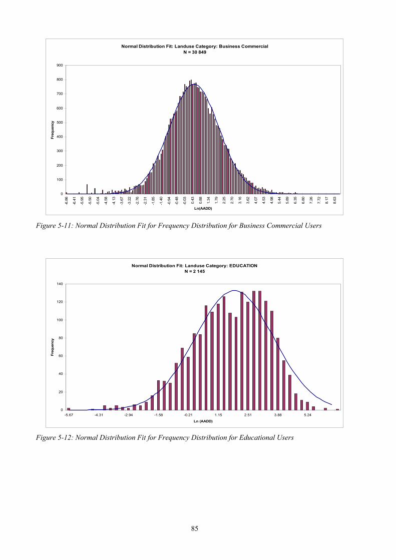
85
Normal Distribution Fit: Landuse Category: Business CommercialN = 30 849
0
100
200
300
400
500
600
700
800
900-6
.86
-6.4
1
-5.9
5
-5.5
0
-5.0
4
-4.5
8
-4.1
3
-3.6
7
-3.2
2
-2.7
6
-2.3
1
-1.8
5
-1.4
0
-0.9
4
-0.4
8
-0.0
3
0.43
0.88
1.34
1.79
2.25
2.70
3.16
3.62
4.07
4.53
4.98
5.44
5.89
6.35
6.80
7.26
7.72
8.17
8.63
Ln(AADD)
Freq
uenc
y
Figure 5-11: Normal Distribution Fit for Frequency Distribution for Business Commercial Users
Normal Distribution Fit: Landuse Category: EDUCATIONN = 2 145
0
20
40
60
80
100
120
140
-5.67 -4.31 -2.94 -1.58 -0.21 1.15 2.51 3.88 5.24
Ln (AADD)
Freq
uenc
y
Figure 5-12: Normal Distribution Fit for Frequency Distribution for Educational Users

86
Normal Distribution Fit: Landuse Category: FarmsN =9 611
0
100
200
300
400
500
600
700
-6.14 -5.44 -4.74 -4.03 -3.33 -2.63 -1.92 -1.22 -0.52 0.19 0.89 1.60 2.30 3.00 3.71 4.41 5.11 5.82 6.52 7.22
Ln(AADD)
Freq
uenc
y
Figure 5-13: Normal Distribution Fit for Frequency Distribution for Farm Users
Normal Distribution Fit: Landuse Category: Government and InstitutionalN = 12 730
0
100
200
300
400
500
600
700
800
900
-6.84 -6.13 -5.43 -4.73 -4.03 -3.32 -2.62 -1.92 -1.22 -0.51 0.19 0.89 1.59 2.30 3.00 3.70 4.40 5.11 5.81 6.51 7.21 7.92 8.62
Ln(AADD)
Freq
uenc
y
Figure 5-14: Normal Distribution Fit for Frequency Distribution for Government and Institutional Users

87
Normal Distribution Fit: Landuse Category: INDUSTRIALN=10 850
0
50
100
150
200
250
300
350
400
450
500-6
.83
-6.0
3
-5.2
4
-4.4
5
-3.6
5
-2.8
6
-2.0
6
-1.2
7
-0.4
8
0.32
1.11
1.91
2.70
3.49
4.29
5.08
5.87
6.67
7.46
8.26
9.05
Ln(AADD)
Freq
uenc
y
Figure 5-15: Normal Distribution Fit for Frequency Distribution for Industrial Users
Normal Distribution Fit: Landuse Category: Sportgrounds and ParksN = 1 099
0
20
40
60
80
100
120
-6.69 -5.84 -4.99 -4.14 -3.29 -2.44 -1.59 -0.74 0.12 0.97 1.82 2.67 3.52 4.37 5.22 6.07
Ln(AADD)
Freq
uenc
y
Figure 5-16: Normal Distribution Fit for Frequency Distribution for Sportgrounds and Parks
The fits for the Government and Institutional, and Educational categories were less good. A
possible reason for this was that the analysis relied heavily on the land use codes assigned by
treasury systems. In both these datasets, it was noted with the data cleaning exercise that the
assignment of land use codes was not consistent for all the municipalities. In other words, what

88
one municipality regarded as an educational facility was regarded as a government institution by
another. It is possible, that further refinement of the land use codes may improve the normal
distribution fits for these two datasets. A direct comparison between the “Red Book” guidelines
and the non-domestic user categories of this study was problematic because the user categories are
not consistent with the “Red Book” categories. Furthermore, the “Red Book” guideline gives the
demand estimate in a unit of gross floor area (m2) and therefore the mean values of the log-normal
distributions could not be compared directly.
The clear log-normal trend, observed in the distributions of the non-domestic user categories, lead
the researchers to use logarithmic regression models during further analysis of the data.
5.2.2 Assessment of Factors Influencing Non-Domestic Water Consumption
There are seven non-domestic user categories and a dataset for each category. On each of these
datasets, a stepwise multiple variable regression analysis was performed. Table 5.6 below
summarises the outcome of the stepwise regression analyses on each category by listing the
independent variables influencing water consumption in each category by order of best correlation
with the AADD. The number of data points in each analysis is also indicated and the adjusted R-
square value of the each stepwise regression model.
Table 5-6: Summary of the Outcome of the Stepwise Multiple Variable Regression Analysis of Non-Domestic Users Categories
Category
Number
of data
points
Number
of
Variables
Independent Variables by order
of Best Correlation with ln
(AADD)
Adjusted R2
LN(Stand Value) 0.23
LN(Stand Area) 0.283
Geographic Location 0.303
Stand Value 0.31
Development Level 0.317
Ave Max Temperature 0.326
Stand Area 0.33
Business
Commercial 24 810 8
Ave Min Temperature 0.332
Ln(Stand Area) 0.408
Development Level 0.422
Stand Value 0.437
Ave Max Temperature 0.455
Education 1 447 5
Ln(Stand Value) 0.458

89
Category
Number
of data
points
Number
of
Variables
Independent Variables by order
of Best Correlation with ln
(AADD)
Adjusted R2
LN(Stand Value) 0.096
Ave Min Temperature 0.113
Stand Area 0.118
Stand Value 0.121
Mean Annual Evaporation 0.122
Farms 8 895 6
Mean Annual Precipitation 0.122
Ln(Stand Area) 0.336
LN(Stand Value) 0.373
Stand Value 0.387
Geographic Location 0.392
Development Level 0.4
Stand Area 0.401
Ave Max Temperature 0.401
Government
and
Institutional
8 259 8
Mean Annual Precipitation 0.401
Ln(Stand Area) 0.313
Stand value 0.33
Geographic Location 0.345
Mean Annual Precipitation 0.35
Stand Area 0.354
Ln(StandValue) 0.36
Ave Max Temperature 0.362
Industrial 8 000 8
Development Level 0.364
Ln(Stand Area) 0.137
Ave Min Temperature 0.176
Development Level 0.191 Parks 367 4
Stand Value 0.207
Ave Min Temperature 0.083 Sports 68 2
Ln(Stand Area) 0.13
As the regression statistics indicate (adjusted R-square values, P-values and t-values) strong
correlations were found between the AADD and the various parameters listed in Table 5.6. The
adjusted R-square values were better on the whole, than those obtained with the multiple variable
regression analyses for domestic use. A possible reason may be that the non-domestic sets were
significantly smaller than the domestic datasets. The Sports category is quite a small dataset and
may be too small to provide statistically significant results.
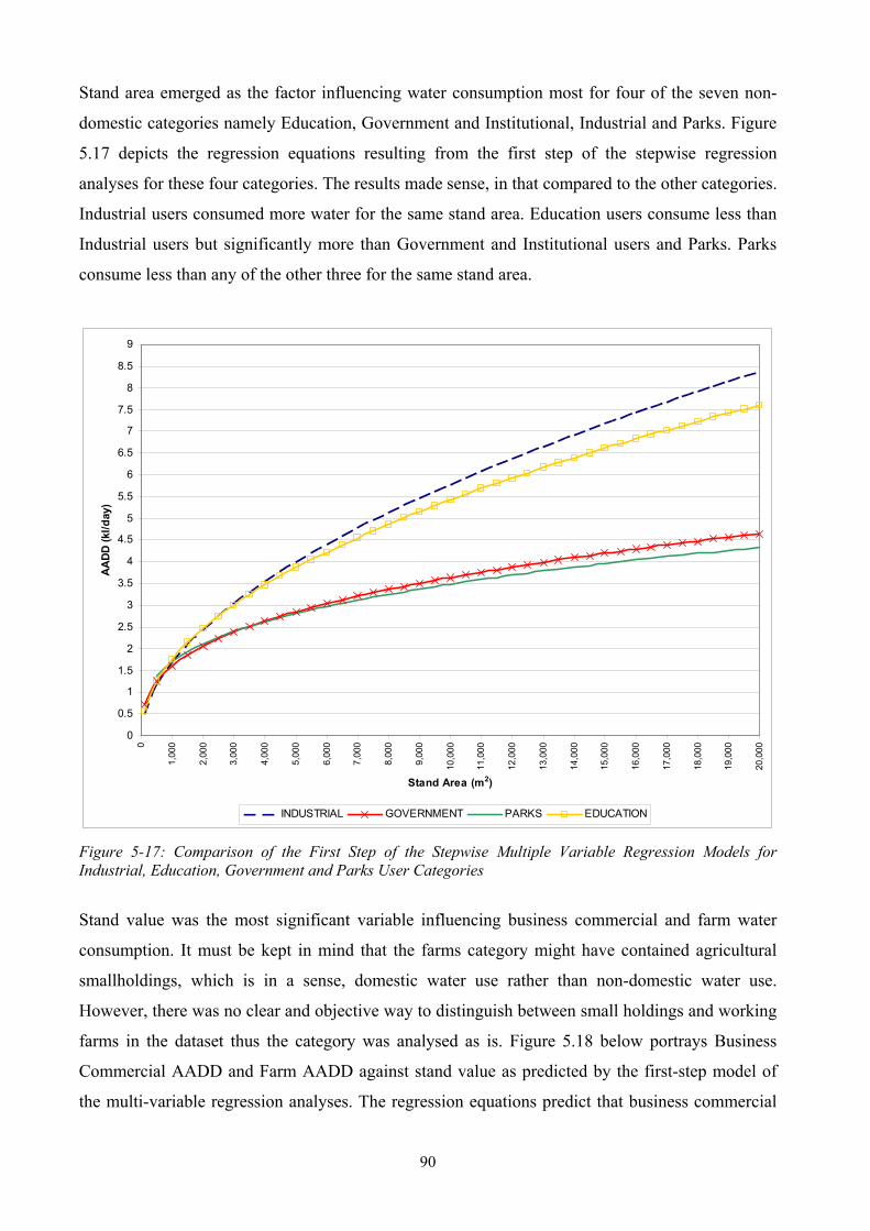
90
Stand area emerged as the factor influencing water consumption most for four of the seven non-
domestic categories namely Education, Government and Institutional, Industrial and Parks. Figure
5.17 depicts the regression equations resulting from the first step of the stepwise regression
analyses for these four categories. The results made sense, in that compared to the other categories.
Industrial users consumed more water for the same stand area. Education users consume less than
Industrial users but significantly more than Government and Institutional users and Parks. Parks
consume less than any of the other three for the same stand area.
0
0.5
1
1.5
2
2.5
3
3.5
4
4.5
5
5.5
6
6.5
7
7.5
8
8.5
9
0
1,00
0
2,00
0
3,00
0
4,00
0
5,00
0
6,00
0
7,00
0
8,00
0
9,00
0
10,0
00
11,0
00
12,0
00
13,0
00
14,0
00
15,0
00
16,0
00
17,0
00
18,0
00
19,0
00
20,0
00
Stand Area (m2)
AADD
(kl/d
ay)
INDUSTRIAL GOVERNMENT PARKS EDUCATION
Figure 5-17: Comparison of the First Step of the Stepwise Multiple Variable Regression Models for Industrial, Education, Government and Parks User Categories
Stand value was the most significant variable influencing business commercial and farm water
consumption. It must be kept in mind that the farms category might have contained agricultural
smallholdings, which is in a sense, domestic water use rather than non-domestic water use.
However, there was no clear and objective way to distinguish between small holdings and working
farms in the dataset thus the category was analysed as is. Figure 5.18 below portrays Business
Commercial AADD and Farm AADD against stand value as predicted by the first-step model of
the multi-variable regression analyses. The regression equations predict that business commercial

91
users and farms consume approximately the same amount of water especially for higher stand
values. At lower stand values, farms consume more water than business commercial users.
00.5
11.5
22.5
33.5
44.5
55.5
6
0
100,
000
200,
000
300,
000
400,
000
500,
000
600,
000
700,
000
800,
000
900,
000
1,00
0,00
0
1,10
0,00
0
1,20
0,00
0
1,30
0,00
0
1,40
0,00
0
1,50
0,00
0
1,60
0,00
0
1,70
0,00
0
1,80
0,00
0
1,90
0,00
0
2,00
0,00
0
Stand Value (R)
AA
DD
(kl/d
ay)
Business Commercial Farms
Figure 5-18: Comparison of the First Step of the Stepwise Multiple Variable Regression Analysis for Business Commercial and Farms User Categories
It should be noted that, in contrast the domestic water consumption analysis, in the non-domestic
consumption analysis stand value was not considered as a proxy for income, but the stand values
were used as an indication of the true monetary value of the sites.
Geographic location (i.e. inland or coastal) did not have the marked impact on non-domestic use as
was the case with domestic use. For only three categories namely, business commercial,
government and institutions and industrial, did geographic location have a significant impact on
the water consumption. The development level (city vs. small town) however, came out as a factor
affecting water consumption for seven of the eight user categories.
As discussed in Chapter 4 (Figure 4.2), the next step in the data analysis was to perform single
variable regressions for stand area, stand value, geographic location and development level. A
summary of the regression equations for the average of all demands with the 95% confidence
intervals are contained in tabular format below.

92
Tabl
e 5-
7: S
ingl
e Va
riab
le R
egre
ssio
n Re
sults
for N
on-D
omes
tic U
ser C
ateg
orie
s with
Dis
tinct
ion
Mad
e fo
r Dev
elop
men
t Lev
el a
nd G
eogr
aphi
c Lo
catio
n
Cat
egor
y D
evel
opm
ent
Lev
el
Geo
grap
hic
Loc
atio
n In
depe
nden
t V
aria
ble
Equ
atio
n N
A
djus
ted
R2
Stan
d A
rea
2602
224
8.7
ln10
1.577.1
260
.2ln
435
.0ln
25
)St
dAre
a(
(Std
Area
)(A
ADD
)
19,6
10
0.23
6 In
land
St
and
Val
ue
3267
003
2.
13ln
101.5
74.142
7.4
ln40
9.0
ln2
5)
StdV
alue
((S
tdVa
lue)
(AAD
D)
19
,610
0.
260
Stan
d A
rea
1984
076
.7ln
106.4
64.177
8.2
ln50
1.0
ln2
4)
StdA
rea
((S
tdAr
ea)
(AAD
D)
2,
192
0.24
4
Met
ro/C
ity
Coa
stal
St
and
Val
ue
3279
247
.13
ln10
6.462
7.1
547
.4ln
401
.0ln
24
)St
dVal
ue(
(Std
Valu
e)(A
ADD
)
2,19
2 0.
258
Stan
d A
rea
2042
328
.7ln
101.5
595
.138
2.2
ln31
2.0
ln2
4)
StdA
rea
((S
tdAr
ea)
(AAD
D)
1,
973
0.20
9 In
land
St
and
Val
ue
2302
860
.12
ln10
1.56.1
328
.4ln
386
.0ln
24
)St
dVal
ue(
(Std
Valu
e)(A
ADD
)
1,97
3 0.
207
Stan
d A
rea
2268
321
.7ln
108.3
53.100
2.2
ln34
0.0
ln2
4)
StdA
rea
((S
tdAr
ea)
(AAD
D)
2,
613
0.14
1
Bus
ines
s C
omm
erci
al
Rur
al/S
mal
l To
wn
Coa
stal
St
and
Val
ue
3269
478
.13
ln10
8.35.1
814
.3ln
319
.0ln
24
)St
dVal
ue(
(Std
Valu
e)(A
ADD
)
2,61
3 0.
179
Stan
d A
rea
2297
54.8ln
101.1
825
.173
9.2
ln48
7.0
ln2
3)
StdA
rea
((S
tdAr
ea)
(AAD
D)
94
2 0.
400
Inla
nd
Stan
d V
alue
16
0033.
13ln
101.1
03.278
6.4
ln46
6.0
ln2
3)
StdV
alue
((S
tdVa
lue)
(AAD
D)
94
2 0.
254
Stan
d A
rea
335
396
.9ln
105.5
156
.276
6.2
ln50
2.0
ln2
3)
StdA
rea
((S
tdAr
ea)
(AAD
D)
18
1 0.
277
Met
ro/C
ity
Coa
stal
St
and
Val
ue
375
292
.14
ln10
5.515
6.2
750
.4ln
469
.0ln
23
)St
dVal
ue(
(Std
Valu
e)(A
ADD
)
181
0.27
0
Stan
d A
rea
742
19.8ln
104.4
67.133
8.3
ln53
1.0
ln2
3)
StdA
rea
((S
tdAr
ea)
(AAD
D)
22
9 0.
556
Educ
atio
n
Rur
al/S
mal
l To
wn
Inla
nd
Stan
d V
alue
72
591
9.
12ln
104.4
65.10.6
ln54
3.0
ln2
3)
StdV
alue
((S
tdVa
lue)
(AAD
D)
22
9 0.
567

93
Cat
egor
y D
evel
opm
ent
Lev
el
Geo
grap
hic
Loc
atio
n In
depe
nden
t V
aria
ble
Equ
atio
n N
A
djus
ted
R2
Stan
d A
rea
323
382
.9ln
106.8
08.233
7.2
ln38
9.0
ln2
3)
StdA
rea
((S
tdAr
ea)
(AAD
D)
11
6 0.
267
Coa
stal
St
and
Val
ue
315
308
.14
ln10
6.813
6.2
864
.3ln
362
.0ln
23
)St
dVal
ue(
(Std
Valu
e)(A
ADD
)
116
0.22
4
Stan
d A
rea
3561
787
.9ln
102.1
41.140
4.1
ln06
5.0
ln2
4)
StdA
rea
((S
tdAr
ea)
(AAD
D)
8,
075
0.00
3 In
land
St
and
Val
ue
5385
520
.12
ln10
2.136
2.1
298
.2ln
245
.0ln
24
)St
dVal
ue(
(Std
Valu
e)(A
ADD
)
8,08
5 0.
076
Stan
d A
rea
659
815
.9ln
104.3
81.155
9.2
ln35
7.0
ln2
3)
StdA
rea
((S
tdAr
ea)
(AAD
D)
29
8 0.
247
Met
ro/C
ity
Coa
stal
St
and
Val
ue
221
906
.11
ln10
3.37.1
504
.7ln
710
.0ln
23
)St
dVal
ue(
(Std
Valu
e)(A
ADD
)
303
0.32
7
Stan
d A
rea
372
319
.10
ln10
8.743.2
449
.2ln
373
.0ln
23
)St
dAre
a(
(Std
Area
)(A
ADD
)
128
0.20
4 In
land
St
and
Val
ue
156
08.13
ln10
6.739.2
562
.6ln
604
.0ln
23
)St
dVal
ue(
(Std
Valu
e)(A
ADD
)
132
-.220
Stan
d A
rea
2082
568
.11
ln10
5.292.1
855
.0ln
149
.0ln
23
)St
dAre
a(
(Std
Area
)(A
ADD
)
402
0.10
5
Farm
s
Rur
al/S
mal
l To
wn
Coa
stal
St
and
Val
ue
3.34
781
7.
12ln
104.2
86.174
5.4
ln43
7.0
ln2
3)
StdV
alue
((S
tdVa
lue)
(AAD
D)
41
1 0.
150
Stan
d A
rea
5150
207
.7ln
108.4
815
.184
3.1
ln34
5.0
ln2
4)
StdA
rea
((S
tdAr
ea)
(AAD
D)
2,
081
0.25
5 In
land
St
and
Val
ue
3842
956
.11
ln10
8.477.1
429
.4ln
424
.0ln
24
)St
dVal
ue(
(Std
Valu
e)(A
ADD
)
2,08
1 0.
288
Stan
d A
rea
1604
7ln
104.1
5.133
1.2
ln39
4.0
ln2
3)
StdA
rea
((S
tdAr
ea)
(AAD
D)
72
0 0.
370
Met
ro/C
ity
Coa
stal
St
and
Val
ue
1341
129
.12
ln10
4.157.1
361
.4ln
395
.0ln
23
)St
dVal
ue(
(Std
Valu
e)(A
ADD
)
720
0.31
0
Gov
ernm
ent
and
Inst
itutio
nal
Rur
al/S
mal
l To
wn
Inla
nd
Stan
d A
rea
5307
28.6ln
106.1
853
.088
1.1
ln33
6.0
ln2
4)
StdA
rea
((S
tdAr
ea)
(AAD
D)
6,
149
0.34
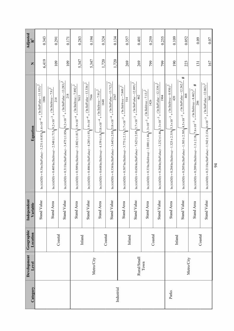
94
Cat
egor
y D
evel
opm
ent
Lev
el
Geo
grap
hic
Loc
atio
n In
depe
nden
t V
aria
ble
Equ
atio
n N
A
djus
ted
R2
Stan
d V
alue
18
0655
3.
11ln
106.1
851
.023
1.3
ln3.0ln
24
)St
dVal
ue(
(Std
Valu
e)(A
ADD
)
6,41
9 0.
343
Stan
d A
rea
214
9.7ln
102.9
715
.154
8.2
ln40
5.0
ln2
3)
StdA
rea
((S
tdAr
ea)
(AAD
D)
10
9 0.
291
Coa
stal
St
and
Val
ue
218
283
.13
ln10
2.985
6.1
475
.3ln
311
.0ln
23
)St
dVal
ue(
(Std
Valu
e)(A
ADD
)
109
0.17
1
Stan
d A
rea
7015
892
.7ln
109.1
817
.188
2.2
ln50
9.0
ln2
4)
StdA
rea
((S
tdAr
ea)
(AAD
D)
5,
347
0.28
3 In
land
St
and
Val
ue
7566
336
.13
ln10
9.193.1
285
.4ln
406
.0ln
24
)St
dVal
ue(
(Std
Valu
e)(A
ADD
)
5,34
7 0.
194
Stan
d A
rea
1648
91.7ln
108.5
8.115
9.4
ln64
8.0
ln2
4)
StdA
rea
((S
tdAr
ea)
(AAD
D)
1,
720
0.32
4
Met
ro/C
ity
Coa
stal
St
and
Val
ue
2547
712
.13
ln10
8.503.2
643
.3ln
336
.0ln
24
)St
dVal
ue(
(Std
Valu
e)(A
ADD
)
1,72
0 0.
134
Stan
d A
rea
514
849
.7ln
107.3
13.277
5.3
ln58
7.0
ln2
3)
StdA
rea
((S
tdAr
ea)
(AAD
D)
26
9 0.
357
Inla
nd
Stan
d V
alue
46
289
5.
12ln
107.3
05.262
3.7
ln65
6.0
ln2
3)
StdV
alue
((S
tdVa
lue)
(AAD
D)
26
9 0.
401
Stan
d A
rea
1426
13.7ln
103.1
46.108
8.2
ln33.0
ln2
3)
StdA
rea
((S
tdAr
ea)
(AAD
D)
79
9 0.
259
Indu
stria
l
Rur
al/S
mal
l To
wn
Coa
stal
St
and
Val
ue
1904
339
.12
ln10
3.146.1
232
.3ln
284
.0ln
23
)St
dVal
ue(
(Std
Valu
e)(A
ADD
)
799
0.25
5
Stan
d A
rea
420
930
.8ln
103.5
319
.232
5.1
ln28
4.0
ln2
3)
StdA
rea
((S
tdAr
ea)
(AAD
D)
19
0 0.
109
Inla
nd
Stan
d V
alue
46
826
2.
12ln
105.4
385
.238
3.1
ln20
5.0
ln2
3)
StdV
alue
((S
tdVa
lue)
(AAD
D)
# 22
3 0.
052
Stan
d A
rea
206
462
.8ln
106.7
18.23.1
ln28
9.0
ln2
3)
StdA
rea
((S
tdAr
ea)
(AAD
D)
#
131
0.09
Park
s
Met
ro/C
ity
Coa
stal
St
and
Val
ue
360
063
.12
ln10
613
4.2
542
.1ln
211
.0ln
23
)St
dVal
ue(
(Std
Valu
e)(A
ADD
)
167
0.07

95
Cat
egor
y D
evel
opm
ent
Lev
el
Geo
grap
hic
Loc
atio
n In
depe
nden
t V
aria
ble
Equ
atio
n N
A
djus
ted
R2
Stan
d A
rea
73.90
21.8ln
1096.1
24.133
5.2
ln32
8.0
ln2
2)
StdA
rea
((S
tdAr
ea)
(AAD
D)
51
0.
314
Inla
nd
Stan
d V
alue
13.
7215
7.
12ln
1089.1
39.182
2.2
ln26
0.0
ln2
2)
StdV
alue
((S
tdVa
lue)
(AAD
D)
53
0.
142
Stan
d A
rea
Sam
ple
size
too
smal
l to
be st
atis
tical
ly si
gnifi
cant
3
n/a
Rur
al/S
mal
l To
wn
Coa
stal
St
and
Val
ue
Sam
ple
size
too
smal
l to
be st
atis
tical
ly si
gnifi
cant
5
n/a
Stan
d A
rea
24.14
064
2.8
ln10
72.113.2
6.0ln
193
.0ln
22
)St
dAre
a(
(Std
Area
)(A
ADD
)
58
0.05
5 In
land
St
and
Val
ue
7.70
145
.13
ln10
72.116.2
877
.1ln
224
.0ln
22
)St
dVal
ue(
(Std
Valu
e)(A
ADD
)#
58
0.03
2 St
and
Are
a Sa
mpl
e si
ze to
o sm
all t
o be
stat
istic
ally
sign
ifica
nt
8 n/
a
Met
ro/C
ity
Coa
stal
St
and
Val
ue
Sam
ple
size
too
smal
l to
be st
atis
tical
ly si
gnifi
cant
8
n/a
Stan
d A
rea
Sam
ple
size
too
smal
l to
be st
atis
tical
ly si
gnifi
cant
3
n/a
Inla
nd
Stan
d V
alue
Sa
mpl
e si
ze to
o sm
all t
o be
stat
istic
ally
sign
ifica
nt
3 n/
a St
and
Are
a Sa
mpl
e si
ze to
o sm
all t
o be
stat
istic
ally
sign
ifica
nt
1 n/
a
Spor
ts
Rur
al/S
mal
l To
wn
Coa
stal
St
and
Val
ue
Sam
ple
size
too
smal
l to
be st
atis
tical
ly si
gnifi
cant
1
n/a
# Eq
uatio
n co
effic
ient
s do
not d
iffer
sign
ifica
ntly
from
zero
.

96
The adjusted R-square values for most of the regression equations indicate strong correlations
between the independent variables stand area and stand value and the AADD, considering that an
adjusted R-square value of more than 20% is considered good, when predicting human behaviour.
The t-statistics and P-values for all the regression coefficients were evaluated to ensure that the
coefficients differ significantly from zero. Where this was not the case, it is indicated in Table 5.7.
These regression models with insignificant coefficients were omitted from any further analysis.
The number of data points (or records) in some categories for the Parks and Sports datasets were
considered to be insufficient to provide statistically significant regression models. The cut-off
point for the minimum number of data points used in this study was 50 data points.
Figures 5.19 to 5.31 represent the regression models for each non-domestic user category.
Appendix C (supplied in electronic format only) contains separate graphs for each model with 95%
confidence intervals for the average AADD indicated.
0
0.5
1
1.5
2
2.5
3
3.5
4
4.5
5
0 250000 500000 750000 1000000 1250000 1500000 1750000 2000000 2250000
Stand Value (R)
AAD
D (k
l/day
)
Metro/City:Inland Metro/City:Coastal Rural/Small Town: Inland Rural/Small Town: Coastal
Figure 5-19: Single Variable Regression Results: AADD vs. Stand Value for Business Commercial Users

97
0
1
2
3
4
5
6
7
8
9
10
0 2000 4000 6000 8000 10000 12000 14000 16000 18000 20000
Stand Area (m2)
AAD
D (k
l/day
)
Metro/City:Inland Metro/City:Coastal Rural/Small Town: Inland Rural/Small Town: Coastal
Figure 5-20: Single Variable Regression Results: AADD vs. Stand Area for Business Commercial Users
0
1
2
3
4
5
6
7
8
9
10
0 500000 1000000 1500000 2000000 2500000
Stand Value (R)
AAD
D (k
l/day
)
Metro/City:Inland Metro/City:Coastal Rural/Small Town: Inland Rural/Small Town: Coastal
Figure 5-21: Single Variable Regression Results: AADD vs. Stand Value for Educational Users

98
0
1
2
3
4
5
6
7
8
9
10
0 2000 4000 6000 8000 10000 12000 14000 16000 18000 20000
Stand Area (m2)
AAD
D (k
l/day
)
Metro/City:Inland Metro/City:Coastal Rural/Small Town: Inland Rural/Small Town: Coastal
Figure 5-22: Single Variable Regression Results: AADD vs. Stand Area for Educational Users
0
2
4
6
8
10
12
14
16
18
0 500000 1000000 1500000 2000000 2500000
Stand Value (R)
AADD
(kl/d
ay)
Metro/City:Inland Metro/City:Coastal Rural/Small Town: Inland Rural/Small Town: Coastal
Figure 5-23: Single Variable Regression Results: AADD vs. Stand Value for Farm Users
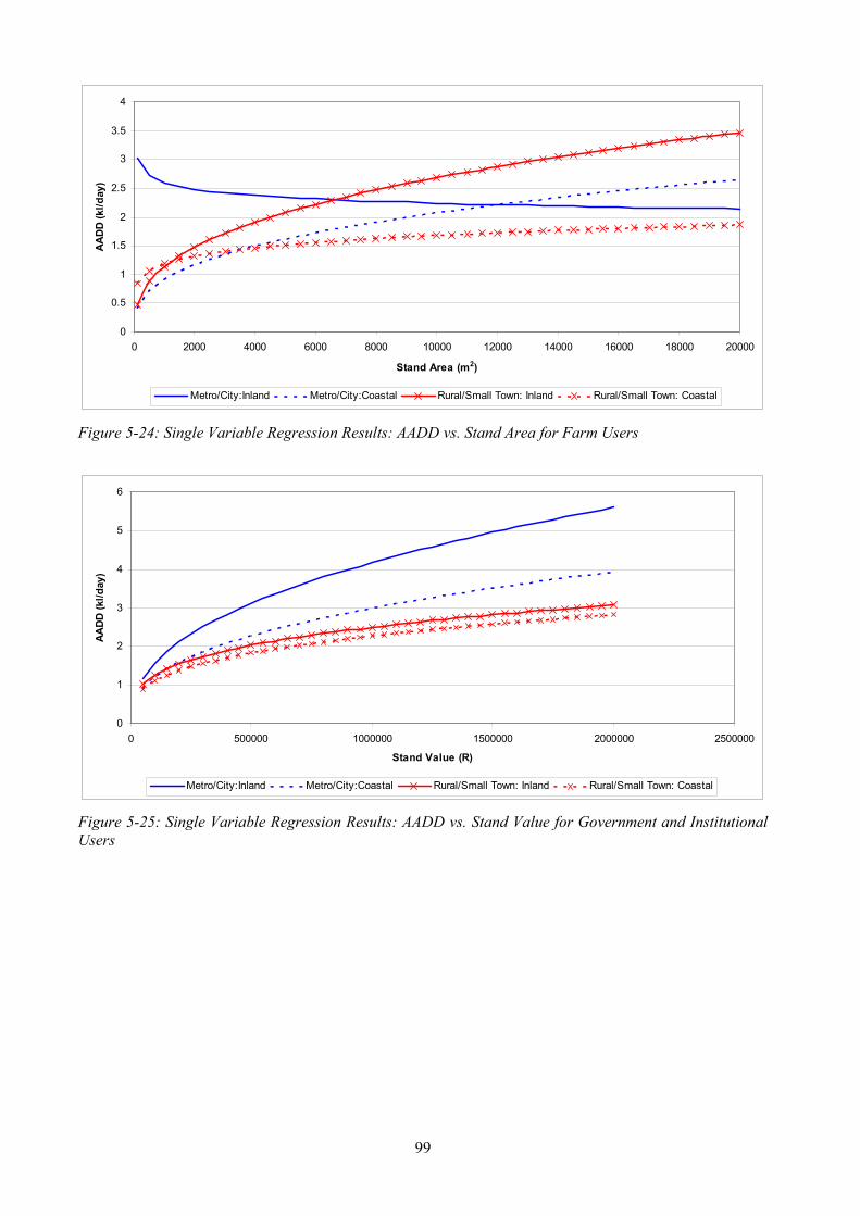
99
0
0.5
1
1.5
2
2.5
3
3.5
4
0 2000 4000 6000 8000 10000 12000 14000 16000 18000 20000
Stand Area (m2)
AAD
D (k
l/day
)
Metro/City:Inland Metro/City:Coastal Rural/Small Town: Inland Rural/Small Town: Coastal
Figure 5-24: Single Variable Regression Results: AADD vs. Stand Area for Farm Users
0
1
2
3
4
5
6
0 500000 1000000 1500000 2000000 2500000
Stand Value (R)
AAD
D (k
l/day
)
Metro/City:Inland Metro/City:Coastal Rural/Small Town: Inland Rural/Small Town: Coastal
Figure 5-25: Single Variable Regression Results: AADD vs. Stand Value for Government and Institutional Users

100
0
1
2
3
4
5
6
0 2000 4000 6000 8000 10000 12000 14000 16000 18000 20000
Stand Area (m2)
AAD
D (k
l/day
)
Metro/City:Inland Metro/City:Coastal Rural/Small Town: Inland Rural/Small Town: Coastal
Figure 5-26: Single Variable Regression Results: AADD vs. Stand Area for Government and
Institutional Users
0
1
2
3
4
5
6
7
0 500000 1000000 1500000 2000000 2500000
Stand Value (R)
AA
DD (k
l/day
)
Metro/City:Inland Metro/City:Coastal Rural/Small Town: Inland Rural/Small Town: Coastal
Figure 5-27: Single Variable Regression Results: AADD vs. Stand Value for Industrial Users
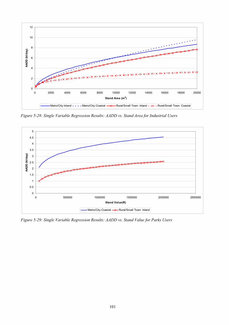
101
0
2
4
6
8
10
12
0 2000 4000 6000 8000 10000 12000 14000 16000 18000 20000
Stand Area (m2)
AAD
D (k
l/day
)
Metro/City:Inland Metro/City:Coastal Rural/Small Town: Inland Rural/Small Town: Coastal
Figure 5-28: Single Variable Regression Results: AADD vs. Stand Area for Industrial Users
0
0.5
1
1.5
2
2.5
3
3.5
4
4.5
5
0 500000 1000000 1500000 2000000 2500000
Stand Value(R)
AAD
D (k
l/day
)
Metro/City:Coastal Rural/Small Town: Inland
Figure 5-29: Single Variable Regression Results: AADD vs. Stand Value for Parks Users

102
0
0.5
1
1.5
2
2.5
3
3.5
4
4.5
5
0 2000 4000 6000 8000 10000 12000 14000 16000 18000 20000
Stand Area (m2)
AAD
D (k
l/day
)
Metro/City:Inland Rural/Small Town: Inland
Figure 5-30: Single Variable Regression Results: AADD vs. Stand Area for Parks Users
0
1
2
3
4
5
6
0 2000 4000 6000 8000 10000 12000 14000 16000 18000 20000
Stand Area (m2)
AAD
D (k
l/day
)
Metro/City:Inland 95% Lower 95% Upper
Figure 5-31: Single Variable Regression Results: AADD vs. Stand Area for Sports Users
From the models, it seemed that the development level might have an impact on the Business
Commercial, Education, Government and Parks user categories in that more water is consumed in
the metropolitan areas than in the rural areas for the same stand area and stand value. However, the
results for farms and industrial were inconsistent with no clear indication whether development
level had any impact. In fact, the results for farms indicated that farms in inland metropolitan areas
did not follow the same trend as the other models at all, namely the model predicted the average
AADD decreases with increasing stand area. The reason may possibly be that for the farms
category the metropolitan areas include more agricultural small holdings than what was the case
for rural areas. Agricultural small holdings should rather be classified as domestic users. Their
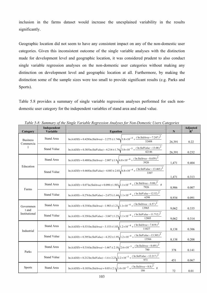
103
inclusion in the farms dataset would increase the unexplained variability in the results
significantly.
Geographic location did not seem to have any consistent impact on any of the non-domestic user
categories. Given this inconsistent outcome of the single variable analyses with the distinction
made for development level and geographic location, it was considered prudent to also conduct
single variable regression analyses on the non-domestic user categories without making any
distinction on development level and geographic location at all. Furthermore, by making the
distinction some of the sample sizes were too small to provide significant results (e.g. Parks and
Sports).
Table 5.8 provides a summary of single variable regression analyses performed for each non-
domestic user category for the independent variables of stand area and stand value.
Table 5-8: Summary of the Single Variable Regression Analyses for Non-Domestic Users Categories
Category Independent
Variable Equation N Adjusted
R2
Stand Area 32408
247.7ln108.3748.1275.2ln428.0ln2
5 )StdArea((StdArea)(AADD) 26,391 0.22 Business
Commercial Stand Value
4214608.13ln108.374.1214.4ln385.0ln
25 )StdValue((StdValue)(AADD)
26,391 0.232
Stand Area 3920
659.8ln108.69.1807.2ln488.0ln2
4 )StdArea((StdArea)(AADD) 1,471 0.404
Education
Stand Value 3307465.13ln108.603.2883.4ln468.0ln
24 )StdValue((StdValue)(AADD)
1,471 0.313
Stand Area 7926
88.9ln101.1503.1098.0ln07.0ln2
4 )StdArea((StdArea)(AADD) # 8,906 0.007 Farms
Stand Value 6298
52.12ln101.144.1673.2ln276.0ln2
4 )StdValue((StdValue)(AADD) 8,934 0.091
Stand Area 13965
57.6ln101.121.1983.1ln354.0ln2
4 )StdArea((StdArea)(AADD) 9,062 0.335 Governmen
t and Institutional Stand Value
12805712.11ln101.123.1847.3ln358.0ln
24 )StdValue((StdValue)(AADD)
9,062 0.314
Stand Area 11027
819.7ln102.183.1153.3ln531.0ln2
4 )StdArea((StdArea)(AADD) 8,138 0.306 Industrial
Stand Value 13566
303.13ln102.195.1252.4ln395.0ln2
4 )StdValue((StdValue)(AADD) 8,138 0.208
Stand Area 780
691.8ln106.218.2667.1ln316.0ln2
3 )StdArea((StdArea)(AADD) 378 0.141 Parks
Stand Value 973
217.12ln102.223.26.1ln212.0ln2
3 )StdValue((StdValue)(AADD) 451 0.067
Sports Stand Area 186
8.8ln104.11.203.0ln103.0ln2
2 )StdArea((StdArea)(AADD) # 72 0.01
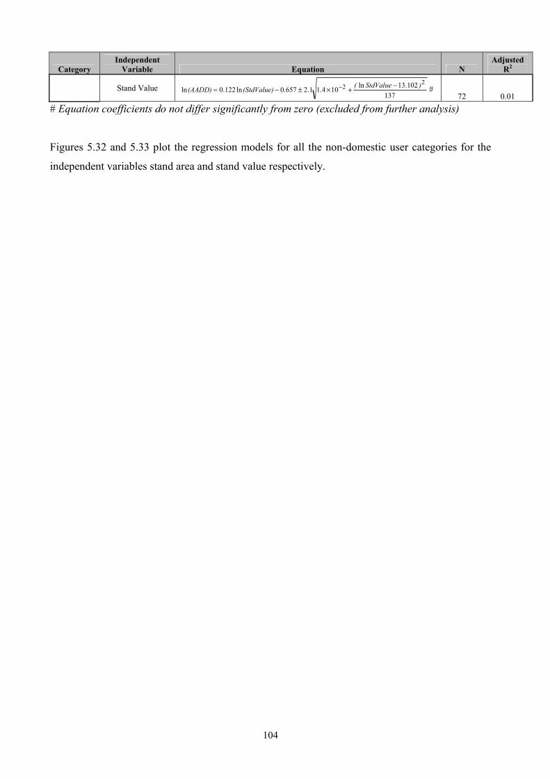
104
Category Independent
Variable Equation N Adjusted
R2
Stand Value 137
102.13ln104.11.2657.0ln122.0ln2
2 )StdValue((StdValue)(AADD) # 72 0.01
# Equation coefficients do not differ significantly from zero (excluded from further analysis)
Figures 5.32 and 5.33 plot the regression models for all the non-domestic user categories for the
independent variables stand area and stand value respectively.

105
6 RETURN FLOW ESTIMATION
6.1 Introduction
There is a direct relationship between water demand and return flow to the sewage reticulation
system. Most indoor demand is returned to the sewer system. Outdoor demand consists mainly of
garden irrigation, and little is thus returned.
6.2 End-use demand and return flow model
The water demand model developed by Jacobs (2004) was used to investigate the return flow of
four user categories: high income, middle income, townships and informal areas. This Microsoft
Excel-based end-use demand model is based on 79 input parameters classified into categories that
include global, monthly, water demand, hot water demand, wastewater, and wastewater salts
parameters. Four output parameters are estimated: total water demand, hot water demand, sewer
return flow and return flow salt content. Only total water demand and sewer return flow was
considered in this study.
To model each user type, a single house was entered in the model and the parameters set to
represent the average values estimated for the user type. The model had to be amended to allow
fractional values to be entered for certain parameters: in the original model, the presence of certain
end-uses, such as swimming pools and washing machines, is entered using a 1 (is present) or 0 (is
not present). However, in this study, this parameter was used to represent the fraction of users in a
category who has a particular type of end-use. Thus, a value of 0.4 for washing machine would
mean that 40% of households in this category used washing machines.
Jacobs did an analysis to determine the most important input variables for the model based on both
the elasticity (how much a change in a parameter affects the model outputs) and sensitivity (how
much variability normally occurs in a parameter) of the parameters. The importance of the
parameters is expressed as a significance index and is given below:
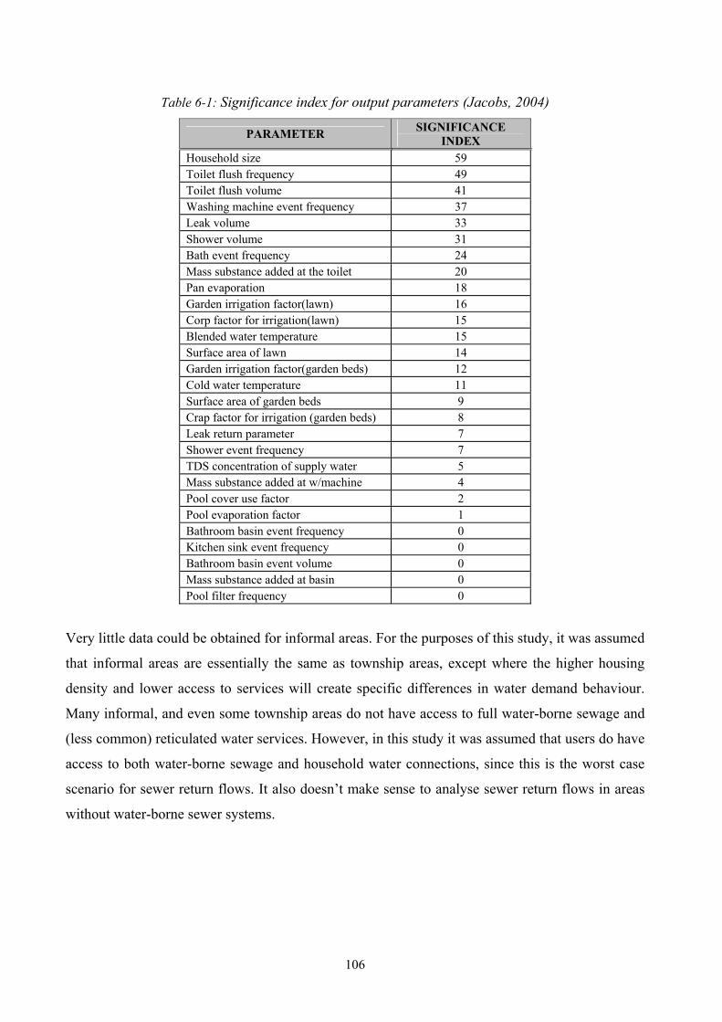
106
Table 6-1: Significance index for output parameters (Jacobs, 2004)
PARAMETER SIGNIFICANCE INDEX
Household size 59 Toilet flush frequency 49 Toilet flush volume 41 Washing machine event frequency 37 Leak volume 33 Shower volume 31 Bath event frequency 24 Mass substance added at the toilet 20 Pan evaporation 18 Garden irrigation factor(lawn) 16 Corp factor for irrigation(lawn) 15 Blended water temperature 15 Surface area of lawn 14 Garden irrigation factor(garden beds) 12 Cold water temperature 11 Surface area of garden beds 9 Crap factor for irrigation (garden beds) 8 Leak return parameter 7 Shower event frequency 7 TDS concentration of supply water 5 Mass substance added at w/machine 4 Pool cover use factor 2 Pool evaporation factor 1 Bathroom basin event frequency 0 Kitchen sink event frequency 0 Bathroom basin event volume 0 Mass substance added at basin 0 Pool filter frequency 0
Very little data could be obtained for informal areas. For the purposes of this study, it was assumed
that informal areas are essentially the same as township areas, except where the higher housing
density and lower access to services will create specific differences in water demand behaviour.
Many informal, and even some township areas do not have access to full water-borne sewage and
(less common) reticulated water services. However, in this study it was assumed that users do have
access to both water-borne sewage and household water connections, since this is the worst case
scenario for sewer return flows. It also doesn’t make sense to analyse sewer return flows in areas
without water-borne sewer systems.

107
6.3 Sources of information
Parameters for the analyses were estimated based on an extensive literature review by Jacobs
(2004), and a market segmentation study commissioned by Rand Water (1999), and a survey on
household water consumption. The first study was conducted in the Gauteng area with the
respondents amounting to 597 adults interviewed personally. The sampling methodology used
ensures that the sample is representative and a 20% back-check was conducted to ensure accuracy
and validity.
The household water consumption survey was conducted on 1 500 users throughout the Rand
Water supply area, and included most of the households surveyed in the market segmentation
study. This data was first filtered by disregarding inconsistent entries and null parameters. With all
unreliable data removed from the data sets, the sets were divided into stand categories namely:
high income, middle income, township and informal areas. The categories boundaries were
determined by distributing the users according to the town type and household income information
included in the questionnaires.
The parameters and selected values are discussed, and are followed by a water demand and return
flow analysis of the study areas.
6.4 Parameters 6.4.1 Household size
Household size refers to the number of people living on a stand. It was the highest scoring
parameter in the ranking exercise and thus has a large influence on the water demand for the
different classes.
From the literature Jacobs (2004) found that high income users have household sizes between 2.6
and 4.7, with an average of 3.3. For townships, household sizes vary between 3.8 and 8.2 with an
average of 6.2. The Rand Water water consumption survey reported household sizes of 4.1, 4.2
and 4.8 for high income, middle income and townships respectively.
This study used household sizes of 3, 4, 6 and 6 for high income, middle income, township and
informal areas respectively. It was assumed that informal areas do not differ significantly from
townships in terms of household size.
108
6.4.2 Bath
From the literature Jacobs (2004) found that the bath volumes vary between 40 and 190 l with an
average of 80 l per event. It was assumed that users in townships and informal areas use a
combination of baths and basin washing, as well as more shared baths, which reduces the effective
bath volume. This study used bath consumptions of 100, 80, 50 and 20 l for high income, middle
income, township and informal areas respectively.
Bath frequency describes the number of times a person takes a bath per day. From the literature
Jacobs (2004) found that the bath frequency varies between 0.22 and 0.9 with an average of 0.24.
The Rand Water water consumption survey reported bath frequencies of 0.5, 0.78 and 0.65 for
high income, middle income and townships respectively.
This study used flush frequencies of 0.6, 0.5, 0.5 and 0.7 for high income, middle income,
township and informal areas respectively. It was assumed that high income areas would have more
access to baths, and thus a higher bathing frequency, while the prevalence of basin washing will be
higher in informal areas.
6.4.3 Shower Shower consumption is determined by both flow rate and duration. From the literature Jacobs
(2004) found that the shower consumption varies between 7.6 and 330 l with an average of 59 l per
shower. This study used shower consumptions of 80, 60, 50 and 40 l for high income, middle
income, township and informal areas respectively.
Shower frequency describes the number of times a person takes a shower per day. From the
literature Jacobs (2004) found that the shower frequencies vary between 0.19 and 0.68 with an
average of 0.31. It was assumed that the average number of baths or showers a person takes per
day is 1.2, 1.1, 1.0 and 1.0 for high income, middle income, township and informal areas
respectively. From these values and the bath frequencies, the shower frequencies were determined
as 0.6, 0.6, 0.5 and 0.3 for high income, middle income, township and informal areas respectively.

109
6.4.4 Toilet Toilet flush frequency describes the number of times a toilet is flushed per user per day. From the
literature Jacobs (2004) found that the toilet flush frequency varies between 0.9 and 5.2 with an
average of 1.9. The Rand Water water consumption survey reported flush frequencies of 4, 3 and
2.8 for high income, middle income and townships respectively. This study used flush frequencies
of 4, 3, 2.5, and 2.5 for high income, middle income, township and informal areas respectively.
Toilet flush volume describes the amount of water used every time a toilet is flushed. Although
dual flush toilets with both large and small flushes are available, these are not common. It was thus
assumed that all toilets use a single large flush only. From the literature Jacobs (2004) found that
the toilet flush volumes vary between 8 and 26.5 l, with an average of 14.3 l. This study used flush
volumes of 15, 15, 12, and 12 l for high income, middle income, township and informal areas
respectively.
6.4.5 Clothes washing Clothes are washed by washing machine or hand. The frequency of clothes washing was assumed
to be independent of how the washing is done, and is described as number of washes per person
per day. From the literature Jacobs (2004) found that the clothes washing frequency varies between
0.12 and 0.63 with an average of 0.3 washes per person per day. The Rand Water water
consumption survey reported clothes washing frequencies of 0.45, 0.33 and 0.25 washes per
person per day for high income, middle income and townships respectively. This study used
clothes washing frequencies of 0.5, 0.3, 0.2, and 0.15 for high income, middle income, township
and informal areas respectively.
The volume of water used per wash was fixed at 120 l for a washing machine. It was assumed that
clothes are mainly washed by machine in high and middle income areas, and by hand in township
and informal areas. This study used clothes washing volumes of 120, 120, 40 and 40 l for high
income, middle income, township and informal areas respectively.
6.4.6 Dishwasher
Dishwashers are mostly found in affluent areas. This study assumed pool ownership of 80, 40, 0
and 0% for high income, middle income, township and informal areas respectively. A fixed
volume of 30 l per wash for dishwashers was assumed. Washing frequencies of 0.5 and 0.4 washes
per person per day were assumed for high and middle income areas respectively.

110
6.4.7 Other volume based demands
Other volume based demands refer to demands not covered explicitly in the end-use model that is
based on a fixed volume of water. Examples include bathroom basins and kitchen sinks. This study
assumed other volume based demands of 30, 30, 20 and 20 l/stand/day for high income, middle
income, township and informal areas respectively. It was assumed that 60% of volume dependent
demands are returned to the sewer system.
6.4.8 Other time based demands
Other time based demands refer to demands not covered explicitly in the end-use model that is
based on a time of use. Examples include car washing and use of free-flowing taps (i.e. basin or
sink not used). This study assumed other time dependent demands of 30, 30, 20 and 20 l/stand/day
for high income, middle income, township and informal areas respectively. It was assumed that
60% of time based demands are returned to the sewer system.
6.4.9 Garden irrigation
The amount of water used for garden irrigation depends on a large number of factors and is
difficult to model. The end-use model uses a number of parameters to estimate garden irrigation,
including irrigation factors, areas of different types of vegetation, crop factors, rainfall and pan
evaporation.
Pan evaporation and rainfall values obtained from the South Africa Weather Services for the
Johannesburg area were used in the study.
A garden irrigation factor is used to compensate for the fact that actual irrigation is rarely the same
as the values obtained by scientific methods. It refers to the fraction of the calculated water
requirement that will be irrigated. This parameter can vary between 0 and 5, with 1 a typical value.
This study used garden irrigation factors of 2, 0.8 and 0.2 for high income, middle income and
township areas respectively.
The crop irrigation factor is used to determine the varying water demand of different crops and
varies with the seasons. The crop irrigation factor for grass (kikuyu or buffalo) was used
throughout in this study.

111
Garden size (stand size excluding house and paved areas) determines the total area that can be
irrigated. This study used garden sizes of 100, 40, 5 and 0 m2 for high income, middle income,
township and informal areas respectively.
6.4.10 Swimming pool
Swimming pools are mostly found in affluent areas. This study assumed pool ownership of 80, 30,
0 and 0% for high income, middle income, township and informal areas respectively.
Pool covers are often used to reduce evaporation and maintenance on pools during the winter
months. It was assumed that 30% of pool owners will have covers in the winter months. The pool
evaporation factor was assumed to be equal to the pan evaporation factor
Pool filters have to be backwashed at regular intervals. From the literature Jacobs (2004) found
that the pool filter backwash frequencies vary between 0.012 and 0.036 with an average of 0.024
backwashes per day. A value of 0.024 backwashes per day and a backwash volume of 150 l were
used in this study.
6.4.11 On-site leakage
On-site leakage is often directed to the sewer system, for instance leaks at a toilet or indoor tap.
From the literature Jacobs (2004) found that on-site leakage varies between 5.8 and 28 l per stand
per day. It was assumed that higher income stands would have better maintenance and thus less
leakage than low income stands. Indoor leakage is normally returned to the sewer system. Return
leakage values of 6, 8, 10 and 10 l/day were used for high income, middle income, township and
informal areas respectively. For leakage not returned to the sewer system, values of 3, 4, 5 and 5
l/day were used for high income, middle income, township and informal areas respectively.
6.4.12 Water temperatures
The cold water temperature varies in direct proportion to the ambient temperature, and was
assumed to vary between 9.7 and 21.7 ºC. The blended water temperature is the ideal water
temperature for a bath or shower. From the literature Jacobs (2004) found that the blended water
temperature varies between 34 and 42.5, with an average of 40.2 ºC. A temperature of 40 ºC was
used throughout this study.
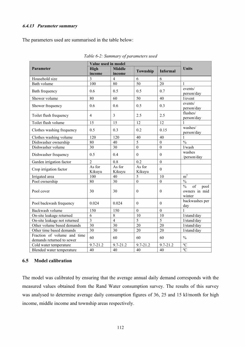
112
6.4.13 Parameter summary
The parameters used are summarised in the table below:
Table 6-2: Summary of parameters used
Value used in model Parameter High
income Middle income Township Informal Units
Household size 3 4 6 6 Bath volume 100 80 50 20 l
Bath frequency 0.6 0.5 0.5 0.7 events/ person/day
Shower volume 80 60 50 40 l/event
Shower frequency 0.6 0.6 0.5 0.3 events/ person/day
Toilet flush frequency 4 3 2.5 2.5 flushes/ person/day
Toilet flush volume 15 15 12 12 l
Clothes washing frequency 0.5 0.3 0.2 0.15 washes/ person/day
Clothes washing volume 120 120 40 40 l Dishwasher ownership 80 40 5 0 % Dishwasher volume 30 30 0 0 l/wash
Dishwasher frequency 0.5 0.4 0 0 washes /person/day
Garden irrigation factor 2 0.8 0.2 0
Crop irrigation factor As for Kikuyu
As for Kikuyu
As for Kikuyu 0
Irrigated area 100 40 5 10 m2 Pool ownership 80 30 0 0 %
Pool cover 30 30 0 0 % of pool owners in mid winter
Pool backwash frequency 0.024 0.024 0 0 backwashes per day
Backwash volume 150 150 0 0 l On-site leakage returned 6 8 10 10 l/stand/day On-site leakage not returned 3 4 5 5 l/stand/day Other volume based demands 30 30 20 20 l/stand/day Other time based demands 30 30 20 20 l/stand/day Fraction of volume and time demands returned to sewer 60 60 60 60 %
Cold water temperature 9.7-21.2 9.7-21.2 9.7-21.2 9.7-21.2 ºC Blended water temperature 40 40 40 40 ºC
6.5 Model calibration
The model was calibrated by ensuring that the average annual daily demand corresponds with the
measured values obtained from the Rand Water consumption survey. The results of this survey
was analysed to determine average daily consumption figures of 36, 25 and 15 kl/month for high
income, middle income and township areas respectively.
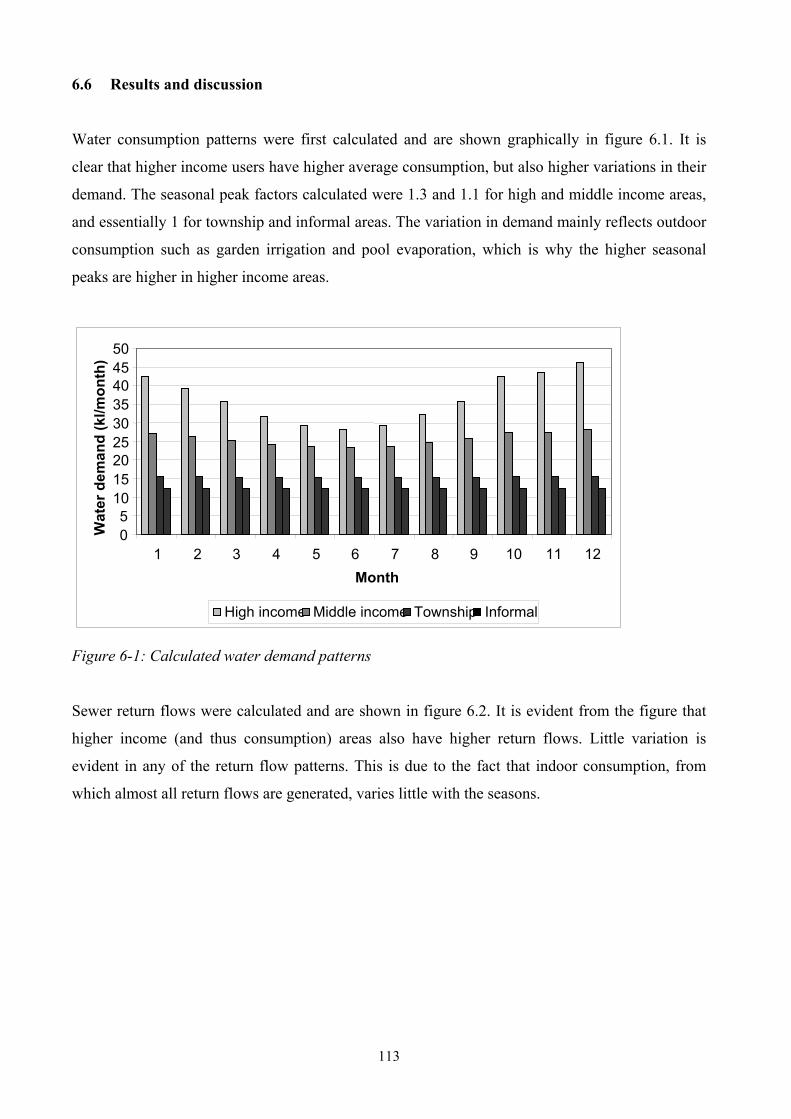
113
6.6 Results and discussion
Water consumption patterns were first calculated and are shown graphically in figure 6.1. It is
clear that higher income users have higher average consumption, but also higher variations in their
demand. The seasonal peak factors calculated were 1.3 and 1.1 for high and middle income areas,
and essentially 1 for township and informal areas. The variation in demand mainly reflects outdoor
consumption such as garden irrigation and pool evaporation, which is why the higher seasonal
peaks are higher in higher income areas.
Figure 6-1: Calculated water demand patterns
Sewer return flows were calculated and are shown in figure 6.2. It is evident from the figure that
higher income (and thus consumption) areas also have higher return flows. Little variation is
evident in any of the return flow patterns. This is due to the fact that indoor consumption, from
which almost all return flows are generated, varies little with the seasons.
0 5
101520253035404550
1 2 3 4 5 6 7 8 9 10 11 12Month
Wat
er d
eman
d (k
l/mon
th)
High income Middle income Township Informal

114
Figure 6-2: Calculated sewer return flow patterns
Finally, the fraction of water demand returned to the sewer system was calculated for the different
user types. The results are shown in figure 6.3. It can be seen from the figure that the highest return
fractions (approximately 97%) are found in township and informal areas. Middle income areas
have significantly lower (average 83%) and high income areas the lowest (average 66%) return
fractions. This is again a reflection of the amounts of water used for outdoor consumption. The
peak factors for the return flows are highest in winter, when the peaks demand are at their lowest,
but are similar in values to the demand peak factors.
Figure 6-3: Fraction of water demand returned to the sewer system
0%10% 20% 30% 40% 50% 60% 70% 80% 90%
100%
1 2 3 4 5 6 7 8 9 10 11 12 Month
Ret
urn
frac
tion
High income Middle income Township Informal
0
5
10
15
20
25
1 2 3 4 5 6 7 8 9 10 11 12Month
Ret
urn
flow
(kl/m
onth
)
High income Middle income Township Informal
115
6.7 Conclusions
This section reported on a study to investigate sewer return flows for four user categories (high
income, middle income, townships and informal areas) using a water demand end-use model
developed by Jacobs (2004). For the purposes of the study, it was assumed that informal areas are
essentially the same as township areas, except where the higher housing density and lower access
to services will create specific differences in water demand behaviour. It was also assumed that all
users, including informal areas, have access to both water-borne sewage and household water
connections, since this is the worst case scenario for sewer return flows.
It was found that both the average water demand and water demand peak increases as the affluence
of areas increases. This is mainly due to higher levels of outdoor consumption in higher affluence
areas.
Sewer return flows are also higher for more affluent areas, but vary little throughout the year. This
is due to the fact that return flow is mainly made up of indoor consumption, which varies little with
the seasons.
The fraction of water consumption that is returned to the sewer decreases as the affluence of areas
increases. The peak return flow is found in the winter months, and is similar in value to the water
demand peak, which is found in the summer months.

116
7 CONCLUSIONS
The main part of this study consisted of an analysis of more than a million individual consumption
records, most of them longer than two years, to estimate the parameters that influence domestic
and non-domestic demands. Climatic and socio-economic census data was also obtained and
linked to the above data. Unfortunately the census data was only available for political wards,
which often include different suburbs with significantly different properties.
An extensive literature review was done of publications and guidelines of water demand in South
Africa. It was found that the most significant parameters that affect domestic water demand are
stand area, household income, water price, available pressure, type of development (suburban vs.
township) and climate. Some work has been done in South Africa regarding the effect of some of
these parameters on water demand, but all these studies were limited in terms of the parameters,
geographical locations and number of data points they considered. A number of previous studies
have shown that the current design guidelines are conservative, especially for larger stands.
Step-wise multiple variable regressions were applied to domestic and non-domestic consumption
data to determine the most significant variables water demand. In a large majority of cases, either
the stand size or stand value had the greatest significance.
The main findings of the domestic demand analyses are as follows:
47% of the average suburb demands fell inside the design envelope proposed by the South
African design guidelines.
Inland water demand is significantly higher than coastal demand.
There is strong evidence that domestic water demand increases with both increasing stand
area and stand value (or income).
Non-domestic users were grouped into seven categories: Business Commercial, Education, Farms,
Government and Institutional, Industrial, Parks and Sports. Good descriptions of all the non-
domestic demand categories could be made using log-normal probability distributions. The
distributions for non-domestic demands are the first produced in South Africa and can form the
basis for rational design guidelines for non-domestic water consumption.

117
Finally, the study investigated sewer return flows from different user types using an end-use
demand model. It was found that high income users show the greatest seasonal variations in both
water demand and fraction of demand returned to the sewer system. This is mainly due to these
users using the largest proportion of water for irrigation purposes. Since most indoor water demand
is returned to the sewer system, and indoor demand shows little seasonal variation, the absolute
sewer flows did not vary much throughout the year.

118
8 REFERENCES
BASSON, M S, VAN NIEKERK, P H, VAN ROOYEN, J A 1997. Overview of Water Resources
Availability and Utilisation in South Africa. Report by Department of Water Affairs and Forestry,
P RSA/00/0197, May.
CITY OF JOHANNESBURG 1989. Water Supply Guidelines for Township Development in
Johannesburg. Water and Gas Department, April.
CSIR 1983. Guidelines for the provision of engineering services in residential townships (Blue
Book). Compiled for the Department of Community Development by the CSIR (SA).
CSIR 1994. Guidelines for the provision of Engineering Services and Amenities in Residential
Township Development (Red Book), Compiled for National Housing Advice Council.
CSIR 2003. Guidelines for human settlement planning and design. A report compiled under the
patronage of the Department of Housing
DANDY D, NQUYEN T, DAVIES C 1997. Estimating Residential Water Demand in the
Presence of Free Allowance. Land Economics 73 (1)
GARLIPP, K D C O .1979. Water Consumption Patterns in urban areas. M.Sc. Dissertation,
University of Pretoria.
HOWE, C W, LINAWEAVER, F P 1967. The impact of Price on Residential Water Demand and
its Relation to System Design and Price Structure. Water Resources Research, 3 (1): 13-32
HUSSELMAN, M L 2004. Estimation of Area and Income Elasticities of Water Demand in a
Number of Cities and Towns in Gauteng. Magister Ingeneriae Dissertation. Rand Afrikaans
University (now University of Johannesburg). August.
JACOBS, H E 2004. A Conceptual End-Use Model for Residential Water Demand and
Return Flow, D.Ing. Thesis, Rand Afrikaans University
119
JACOBS, H E, GEUSTEYN, L C, LOUBSER, B F, VAN DER MERWE, B 2004. Estimating
residential water demand in Southern Africa. Journal of the South African Institution of Civil
Engineering, 46(4): 2-13, Paper 568
MIDGLEY DC, PITMAN WV, MIDDLETON BJ. 1994. Surface Water Resources of South
Africa, WRC Report No 298/1/94, User Manual. ISBN 1 86845 143 7 and all the subsequent
volumes.
RAND WATER, 1999. Consumer Market Segmentation Study, Report EG03, Rand Water
Marketing Department, Johannesburg
STEPHENSON, D AND TURNER, K 1996. Water demand patterns in Gauteng. IMIESA, 21 (1):
11-16
VAN VUUREN, S J, VAN BEEK, J C, 1997, Her-Evaluering van die Bestaande Riglyne vir
Stedelike en Industriele Watervoorsiening gebaseer op Gemete Waterverbruike Fase 1: Pretoria
Voorsieningsgebied, Report for the Water Research Commission by the Department of Civil
Engineering, University of Pretoria, WRC Report No 705/1/97.
VAN ZYL, J E, HAARHOFF, J, HUSSELMAN, M L 2003. Potential application of end-use
demand modelling in South Africa. Journal of the South African Institution of Civil Engineering,
45(2): 9-19.
VECK, G A, BILL, M R, 2000. Estimation of the Residential Price Elasticity of Demand for Water
by means of a contingent valuation approach. Report for the Water Research Commission of South
Africa. WRC Report No. 790/1/00.
WATER TRANSFER CONSULTANTS 2001. Central Area System Update: Determination of the Current
and Forecasted Water Demands for the Central Area of Namibia. Report compiled December 2001.
WCE, ENVES, EPE and CSIR 2003. Economic feasibility study on the artificial recharge of the Windhoek
Aquifer. Report compiled June 2003.