The Joint Institute for Strategic Energy Analysis is operated by the Alliance for Sustainable Energy, LLC, on behalf of the U.S. Department of Energy’s National Renewable Energy Laboratory, the University of Colorado-Boulder, the Colorado School of Mines, the Colorado State University, the Massachusetts Institute of Technology, and Stanford University.

Contract No. DE-AC36-08GO28308

Waste Not, Want Not: Analyzing the Economic and Environmental Viability of Waste-to-Energy (WTE) Technology for Site-Specific Optimization of Renewable Energy Options Kip Funk National Renewable Energy Laboratory

Jana Milford University of Colorado at Boulder

Travis Simpkins National Renewable Energy Laboratory

Technical Report NREL/TP-6A50-52829 February 2013

The Joint Institute for Strategic Energy Analysis is operated by the Alliance for Sustainable Energy, LLC, on behalf of the U.S. Department of Energy’s National Renewable Energy Laboratory, the University of Colorado-Boulder, the Colorado School of Mines, the Colorado State University, the Massachusetts Institute of Technology, and Stanford University.

JISEA® and all JISEA-based marks are trademarks or registered trademarks of the Alliance for Sustainable Energy, LLC.

The Joint Institute for Strategic Energy Analysis 15013 Denver West Parkway Golden, CO 80401 303-275-3000 • www.jisea.org Contract No. DE-AC36-08GO28308

Waste Not, Want Not: Analyzing the Economic and Environmental Viability of Waste-to-Energy (WTE) Technology for Site-Specific Optimization of Renewable Energy Options Kip Funk National Renewable Energy Laboratory

Jana Milford University of Colorado at Boulder

Travis Simpkins National Renewable Energy Laboratory

Prepared under Task Nos. 6A50.2012, 6A50.2001

Technical Report NREL/TP-6A50-52829 February 2013

NOTICE

This report was prepared as an account of work sponsored by an agency of the United States government. Neither the United States government nor any agency thereof, nor any of their employees, makes any warranty, express or implied, or assumes any legal liability or responsibility for the accuracy, completeness, or usefulness of any information, apparatus, product, or process disclosed, or represents that its use would not infringe privately owned rights. Reference herein to any specific commercial product, process, or service by trade name, trademark, manufacturer, or otherwise does not necessarily constitute or imply its endorsement, recommendation, or favoring by the United States government or any agency thereof. The views and opinions of authors expressed herein do not necessarily state or reflect those of the United States government or any agency thereof.

Available electronically at http://www.osti.gov/bridge

Available for a processing fee to U.S. Department of Energy and its contractors, in paper, from:

U.S. Department of Energy Office of Scientific and Technical Information

P.O. Box 62 Oak Ridge, TN 37831-0062 phone: 865.576.8401 fax: 865.576.5728 email: mailto:reports@adonis.osti.gov

Available for sale to the public, in paper, from:

U.S. Department of Commerce National Technical Information Service 5285 Port Royal Road Springfield, VA 22161 phone: 800.553.6847 fax: 703.605.6900 email: orders@ntis.fedworld.gov online ordering: http://www.ntis.gov/help/ordermethods.aspx

Cover Photos: (left to right) PIX 12721, PIX 13995, © GM Corp., PIX 16161, PIX 15539, PIX 16701

Printed on paper containing at least 50% wastepaper, including 10% post consumer waste.

iv

List of Acronyms and Abbreviations AD anaerobic digestion BACT Best Available Control Technology BOS balance of system Btu British thermal unit Cd cadmium CDD/CDF dioxin/furan CEMS continuous emissions monitoring systems CHP combined heat and power CO carbon monoxide CO2 carbon dioxide CO2-e CO2-equivalent dscm dry standard cubic meter EPA Environmental Protection Agency GCS geographic coordinate system GHG greenhouse gas GIS geographical information system HCl hydrogen chloride Hg mercury HRSG heat-recovery steam generator JISEA Joint Institute for Strategic Energy Analysis Kg kilogram kW kilowatt kWh kilowatt hour LAER Lowest Achievable Emissions Rate LCA life cycle assessment MACT maximum achievable control technology µg microgram mg milligram MMBtu million British thermal units MSW municipal solid waste MSW-DST Municipal Solid Waste Decision Support Tool MW megawatt MWC municipal waste combustor NIST National Institute of Standards and Technology NOx nitrogen oxides NREL National Renewable Energy Laboratory NSPS New Source Performance Standards NSR New Source Review O&M operations and maintenance Pb lead PM particulate matter ppm parts per million PSD Prevention of Significant Deterioration psig pounds per square inch gauge RDF refuse-derived fuel

v

RE renewable energy REC Renewable Energy Credit REO renewable energy optimization RSC Rankine steam cycle RTI Research Triangle Institute SCR selective catalytic reduction SNCR selective noncatalytic reduction SO2 sulfur dioxide TPD tons per day TPH tons per hour WTE waste-to-energy

vi

Executive Summary Waste-to-energy (WTE) technology burns municipal solid waste (MSW) in an environmentally safe combustion system to generate electricity, provide district heat, and reduce the need for landfill disposal. While this technology has gained acceptance in Europe, it has yet to be commonly recognized as an option in the United States.

Section 1 of this report provides an overview of WTE as a renewable energy (RE) technology and describes a high-level model developed to assess the feasibility of WTE at a site. The model uses simple user inputs, geographic information system (GIS)-based waste resource data, available incentives, and financial parameters to estimate implementation cost, operations costs, and life-cycle cost, along with the recommended quantities of WTE to consider. The development of this model and integration in the National Renewable Energy Laboratory’s (NREL) Renewable Energy Optimization (REO) tool allows WTE to be considered alongside other RE options and helps to introduce the technology to a broad audience.

Section 2 of this report reviews results from previous life cycle assessment (LCA) studies of WTE that have been published in the literature, and then uses an existing LCA inventory tool to perform a screening-level analysis of cost, net energy production, greenhouse gas (GHG) emissions, and conventional air pollution impacts of WTE for residual MSW in Boulder, Colorado. We find that MSW combustion is a better alternative than landfill disposal in terms of net energy impacts and carbon dioxide (CO2)-equivalent GHG emissions. In this report, WTE leads to greater GHG reductions per kWh of electricity generated compared to landfill gas-to-energy. The screening indicates WTE would be a relatively expensive way to treat Boulder’s residual MSW, at an estimated cost of about $58 per ton (higher than typical landfill costs for this region).

Section 3 of this report describes the federal regulations that govern the permitting, monitoring, and operating practices of MSW combustors and provides emissions limits for WTE projects.

vii

Table of Contents List of Figures .......................................................................................................................................... viii List of Tables ............................................................................................................................................ viii 1 Waste-to-Energy Model for NREL’s Renewable Energy Optimization Tool ................................... 1

1.1 Introduction ...................................................................................................................................... 1 1.2 Background ...................................................................................................................................... 1

1.2.1 Renewable Energy Optimization ........................................................................................ 1 1.2.2 Waste-to-Energy History .................................................................................................... 1 1.2.3 Waste Management Practices ............................................................................................. 2 1.2.4 Waste-to-Energy Overview ................................................................................................ 3

1.3 Waste-to-Energy Heating, Electrical Generation, and CHP Technologies ...................................... 5 1.3.1 Overview of Technology .................................................................................................... 5 1.3.2 Feedstock Characterization ................................................................................................. 6 1.3.2.1 Municipal Solid Waste .................................................................................................... 6 1.3.2.2 Other Dry and Wet Wastes ............................................................................................. 7 1.3.3 Feedstock Conversion Technologies .................................................................................. 8 1.3.3.1 Combustion ..................................................................................................................... 8 1.3.3.2 Gasification .................................................................................................................... 8 1.3.3.3 Pyrolysis ......................................................................................................................... 9 1.3.3.4 Anaerobic Digestion ....................................................................................................... 9

1.4 Methods for Energy Recovery ....................................................................................................... 10 1.4.1 Heat Recovery ................................................................................................................... 10 1.4.1.1 Solid Fuels .................................................................................................................... 10 1.4.1.2 Synthesis Gas ................................................................................................................ 10 1.4.2 Power Generation ............................................................................................................. 10 1.4.3 Pipeline Injection .............................................................................................................. 11

1.5 Renewable Energy Optimization WTE Analysis Module ............................................................. 11 1.5.1 Calculation of Electrical Load Met by WTE .................................................................... 12 1.5.2 Calculation of Thermal Load Met by WTE ...................................................................... 12 1.5.3 Calculation for CHP .......................................................................................................... 13 1.5.4 Calculation of WTE Consumption .................................................................................... 14 1.5.5 Annual Fixed and Variable Operations & Maintenance Cost ........................................... 14 1.5.6 Calculation of Capital Cost ............................................................................................... 14

2 Life Cycle Assessments for Municipal Waste Combustion ........................................................... 16

2.1 Introduction .................................................................................................................................... 16 2.2 Methods ......................................................................................................................................... 17 2.3 Results ............................................................................................................................................ 20 2.4 Conclusions .................................................................................................................................... 25 References ............................................................................................................................................ 26

3 Air Emissions Limits for Municipal Waste Combustors ................................................................ 28

Reference .............................................................................................................................................. 32 Appendix A: Description of Municipal Solid Waste in the Renewable Energy Optimization GIS Data

Tool ...................................................................................................................................................... 33 Introduction .......................................................................................................................................... 33 What REO GIS Does ............................................................................................................................ 33 How to Use REO GIS .......................................................................................................................... 33

viii

Web-Based Tool ............................................................................................................................ 34 Single Lookup Point .................................................................................................................. 34 Multiple Lookup Points ............................................................................................................. 34

REO Data Services ........................................................................................................................ 34 Output and Data Sources ...................................................................................................................... 35 MSW Analysis Example Figures ......................................................................................................... 36 Contact Us ............................................................................................................................................ 39

List of Figures Figure 1-1. EPA solid waste management hierarchy. ............................................................................. 3 Figure 1-2. Energy pathways for WTE. ..................................................................................................... 4 Figure 1-3. Breakdown of MSW generated in the United States in 2010. .............................................. 7 Figure 1-4. Direct combustion system. ..................................................................................................... 8 Figure 1-5. McNeil Generating Station in Burlington, Vermont, uses gasification technology to

convert wood chips to power. ............................................................................................................. 9 Figure 1-6. User input. .............................................................................................................................. 11 Figure 1-7. Electrical efficiency (net) % vs. kW. ..................................................................................... 12 Figure 1-8. Boiler efficiency (net) percentage vs. boiler output (MMBtu). .......................................... 13 Figure 1-9. CHP performance: net electrical efficiency vs. net boiler efficiency. .............................. 14 Figure 2-1. Percentages of fossil CO2 emissions produced in each stage of MSW management for

Boulder. ............................................................................................................................................... 22

List of Tables Table 1-1. Biomass Conversion Technologies Summary ....................................................................... 6 Table 2-1. Residual MSW Production Rates and Waste Collection Points for Boulder .................... 18 Table 2-2. Residual MSW Composition for Boulder .............................................................................. 19 Table 2-3. Estimated Impacts of Combustion Stage of WTE for Boulder MSW ................................. 21 Table 2-4. Sensitivity of Direct WTE Facility Impacts to System Efficiency ....................................... 22 Table 2-5. Comparison of WTE Combustion Stage Impacts for Boulder MSW with Impacts for

National Default Residential MSW .................................................................................................... 23 Table 2-6. Comparison of Emissions Rates for WTE with Ash Disposal vs. Landfill

Gas-to-Energy ..................................................................................................................................... 24 Table 2-7. Comparison of Estimated Impacts of WTE vs. Landfill Disposal for Boulder MSW ........ 25 Table 3-1. Federal Emission Limits (NSPS) for Large MWC Units Constructed After December

19, 2005 (71 FR 27324, 27326) ........................................................................................................... 29 Table 3-2. Emission Limits for MSW Combustion Facilities Reported in the RACT/BACT/LAER

Clearinghouse and Associated Air Permits ..................................................................................... 30

1

1 Waste-to-Energy Model for NREL’s Renewable Energy Optimization Tool

1.1 Introduction This section provides an overview of waste-to-energy (WTE) as a renewable energy (RE) technology and describes how the Renewable Energy Optimization (REO) tool utilizes available data to identify at a high level WTE feasibility in a user-defined location. The model estimates the energy generation and costs, and recommends a system size that minimizes life-cycle cost of energy for the site. Thermal, electric, and combined heat and power (CHP) production can all be analyzed with this module.

The tool utilizes user inputs and geographical information system (GIS) data on WTE resources at particular sites and analyzes the potential for WTE technologies to be utilized, along with other RE technologies. Determining whether WTE is cost effective requires modeling the integrated system based on the details of the site, the different WTE technologies and their application, available incentives, and financial parameters. The model yields estimated implementation costs, operations costs, and life-cycle cost, along with the recommended quantities of WTE to consider.

REO determines the scale of a project through consideration of both small, distributed building measures (kW scale) and central plant measures on the scale a campus or community (MW scale). The optimal size of each measure is estimated using optimization software. Note that the capital and operating costs calculated are based on national averages for large projects and are not specific to any particular locations1.

1.2 Background 1.2.1 Renewable Energy Optimization The REO tool, developed by NREL, identifies the combination of RE technologies that minimize life-cycle cost of energy for a particular site and set of constraints. The optimization problem is couched in three terms: an objective, the variables, and the constraints. Typically the objective is to minimize life-cycle cost of energy. The variables are the size of each RE project on each site. Constraints, such as percent energy from renewable, available land area, available capital expenditure, etc., can be included in the analysis. The objective of the REO analysis is to quantitatively evaluate multiple scenarios leading to the recommendation of a specific project for more detailed engineering analysis.

1.2.2 Waste-to-Energy History The first U.S. WTE facility was built in New York in 1898. The Clean Air Act of 1970 and the rise in oil prices led to a growth in WTE facilities through the 1970s. Since then, however, WTE

1 True costs may vary from national averages for several reasons. Existing WTE tipping fees include old debt service based on old CAPEX—new WTE plants cost more. Furthermore, if privately owned, the tipping fees are market, not cost, based. For landfills, tipping fees are generally market based unless publicly owned. At publicly owned landfills, tipping fees cover unfunded mandates such as recycling, household hazardous waste, and electronics. Also, to get to a landfill, transfer (by truck or rail) often adds additional costs.

2

has slowed in the United States. No new facilities have been built in over 10 years, although the technology is prevalent in Europe and Asia.2 Compared to WTE facilities of the 1970s and 80s, WTE is now a refined, clean, well-managed application for energy production. The Clean Air Act of 1990 defined and regulated the emissions from a WTE facility to be the most stringent in the world. Public perception, based on the poor emission controls of WTE facilities through the 1980s, has been that WTE facilities are “dirty,” and the common theme has been to stop the development of WTE facilities. Success of WTE plants today is highly dependent on local costs of waste disposal, electricity value, heat value, and the public’s acceptance. 1.2.3 Waste Management Practices Waste management practices have also changed since the early 1970s. Many communities as well as local and state governments have implemented zero-waste strategies, where they utilize the reduce, reuse, recycle, and compost (or 3RC) strategy, WTE, and landfill as a path to minimize the potential for pollution of air and ground water. See Figure 1-1 for EPA’s Recycling/Energy Recover Solid Waste Management Hierarchy. Many communities and government organizations have concluded that zero waste is currently unattainable. A major effort to minimize packaging of marketed items is being made through changing policy. Recycling efforts are also being implemented successfully by many organizations. Currently California has a goal of 50% waste reduction, which the state is meeting, and some communities are exceeding substantially3.

2 Meeting the Future: Evaluating the Potential of Waste Processing Technologies to Contribute to the Solid Waste Authority’s System. Solid Waste Authority of Palm Beach County, Florida. http://swa.org/pdf/SWAPBC_White_Paper_9-2-09.pdf. 3 “California Recycling Laws: CA Integrated Waste Management Act of 1989 (AB 939).” Californians Against Waste. www.cawrecycles.org/facts_and_stats/california_recycling_laws.

3

Source: EPA, http://www.epa.gov/garbage/faq.htm#1

Figure 1-1. EPA solid waste management hierarchy.

Reduction of greenhouse gasses (GHGs) is another consideration during the life-cycle evaluations of waste management practices. Some communities are far enough away from the recycle markets that some of the recyclable materials are not economically and environmentally justified to include as part of their near-term recycle goals. The carbon footprint can potentially increase due to shipping materials to the market, compared to utilizing the recyclable material as a feedstock for a WTE facility or to continue sending the material to a landfill. 1.2.4 Waste-to-Energy Overview Waste-to-energy technologies consist of various methods for extracting energy from waste materials. These methods include thermochemical and biological methods. Figure 1-2 provides an illustration of the various energy pathways for WTE. Of these pathways, most are in early developmental stages. Currently the WTE technologies that are commercially proven in the United States using MSW feedstock are combustion and anaerobic digestion. All other processes hold high potential for utilizing MSW feedstock but must overcome various technical, institutional, economic, environmental, and/or procedural challenges to become commercially viable. The primary challenge facing these technologies is the heterogeneous nature of MSW, which creates a widely varying chemical constituency of the energy products generated from these processes. This variance affects the ability to efficiently extract energy. Solutions are actively being pursued from two angles.

1. Cleanup and conditioning of synthetic gas (syngas) products of thermochemical

conversion and biogas products of biological conversion. These efforts are directed at making the gases more usable as a direct fuel in internal combustion engines or gas turbines, and for pipeline injection.

4

2. Feedstock preparation, shredding, and/or mixing MSW to make the feedstock more homogeneous. This homogeneity will be reflected in the energy product(s) and help improve its utility.

Permitting of MSW conversion technologies is also a major challenge. Permitting is arduous and complex, especially in California. Technologies utilized as part of the criteria for recycling and energy generation include anaerobic digestion, combustion, gasification, and pyrolysis. These technologies can be combined, and are used with emission control equipment and monitoring systems to substantially reduce emissions to meet the stringent air emission limits established through the permitting process with the specific Environmental Protection Agency (EPA) air district and local air management district in each state.

Figure 1-2. Energy pathways for WTE.

The scope of this task includes the development of a characterization of waste resources to be utilized for the evaluation and optimization of WTE technologies as a component of the REO portfolio. The WTE technologies considered include anaerobic digestion (AD), combustion, gasification, and pyrolysis for heat, electricity, and CHP.

5

1.3 Waste-to-Energy Heating, Electrical Generation, and CHP Technologies

1.3.1 Overview of Technology Waste-to-energy is widely used for facility heating, electric power generation, and CHP. The term “waste-to-energy” encompasses a large variety of materials including MSW, commercial waste, used tires or non-recycled components of tires, sanitary waste, food waste, and agricultural residues, etc. WTE is typically included within the definition of biomass, but for the purposes of this document, we will only consider waste stereotypical of MSW.

Waste-to-energy is commonly used for energy generation in the form of steam, electricity, or a combination of both, in several forms: raw unprocessed mass feed, refuse-derived fuels, industrial waste, medical waste, waste tires, food waste, and high organic waste.

The use of MSW to produce heat or power can be divided into four main activities: 1) resource receiving (receiving waste and collecting a tipping fee); 2) storage, processing, and conveyance; 3) conversion to thermal or electrical energy (combustion, thermal conversion, or biochemical conversion, which is ultimately used to produce heat or to drive a steam turbine, gas turbine, or internal combustion engine); and 4) distribution of the thermal or electrical energy.

Several technologies are available to convert MSW feedstocks into heat and electricity. These include direct combustion, gasification, pyrolysis, and anaerobic digestion. Of the several technologies for converting MSW to energy, mass burn4 is the most common, which directly combusts MSW as a fuel with minimal processing. “Refuse-derived fuel” is a term for loose or pelletized fuel derived from processed waste, which is then burned on its own, or is co-fired with other fuels (like coal). Other MSW technologies include pyrolysis and thermal gasification, where waste is decomposed at a high temperature with little or no oxygen in order to generate a producer gas, which can then be combusted to generate heat and electricity using a boiler and steam turbine or using a combustion engine or combustion turbine. Pyrolysis technology is still under development.

Table 1-1 provides a summary of biomass conversion technologies, including the mode of operation, current status, and commercial availability.

4 There are three types of mass burn: refractory lined, water-wall lined, and modular smaller systems. Refractory systems have higher capital and operating costs; water-wall lined systems have higher capital and lower operating costs; and modular systems have lower capital but higher operating costs.

6

Table 1-1. Biomass Conversion Technologies Summary

Technology Description Mode of Operation Commercially Available for WTE

Combustion Thermal conversion of a feedstock utilizing excess air or oxygen as oxidant to generate heat.

-Grate -Bubbling fluidized bed -Circulating fluidized bed

87 installations in the United States

Pyrolysis Thermal conversion of a feedstock in the absence of air or oxygen as oxidant to generate a synthesis gas or fuel and pyrolysis oil. (Plasma arch capabilities of operating in excess of 20,000ºF.)

-Horizontal -Vertical (updraft/downdraft) -Plasma arch

Two installations in the United States

Gasification Thermal conversion of feedstock in a limited atmosphere of air or oxygen as oxidant to generate a synthesis gas or fuel.

-Horizontal stationary -Horizontal rotating -Vertical (updraft/downdraft) -Stationary grate -Bubbling fluidized bed

0 installations in the United States

Anaerobic Digestion Biochemical conversion of a feedstock in the absence of oxygen to generate biogas.

-Mesophilic (77ºF–100ºF) -Thermophilic (122ºF–135ºF)

Multiple installations in the United States (total quantity unknown)

1.3.2 Feedstock Characterization Sources of waste from the specific sites and from the surrounding area are considered to determine feedstock inventory of waste streams. Common waste streams are described below. A wide variety of feedstocks can be used, with the only limitation that they are carbon-based substances.

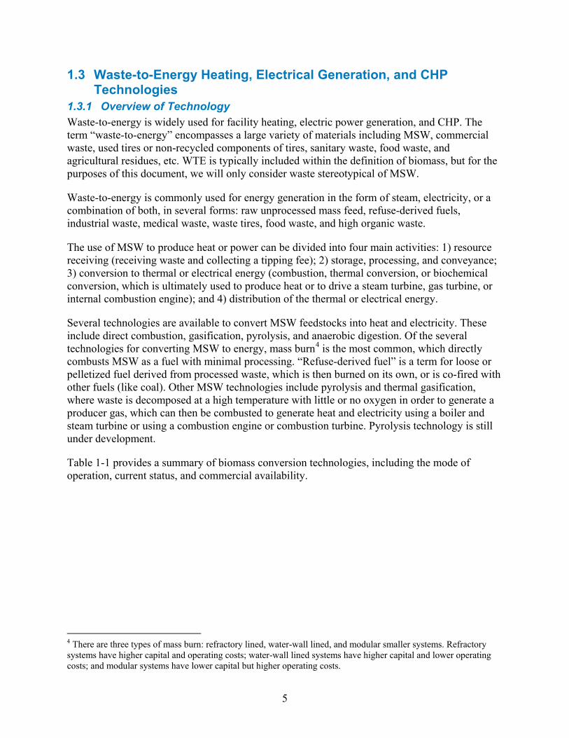
1.3.2.1 Municipal Solid Waste Municipal solid waste is commonly known as trash or garbage. In 2010, 250 million tons of MSW were generated in the United States.5 Municipal solid waste includes organic wastes such as paper, cardboard, food, yard trimmings, and plastics, and inorganic wastes such as metal and glass. Figure 1-3 shows the breakdown of MSW generated in the United States in 2010.

5 “Municipal Solid Waste.” Environmental Protection Agency (EPA). Accessed September 12, 2012: http://www.epa.gov/epawaste/nonhaz/municipal/index.htm.

7

Source: EPA, http://www.epa.gov/epawaste/nonhaz/municipal/images/index_pie_chrt_900px.jpg

Figure 1-3. Breakdown of MSW generated in the United States in 2010.

1.3.2.2 Other Dry and Wet Wastes Other sources of dry (i.e., high-solids) biomass include crop residue, orchard prunings, forest residue, and primary mill residue, among others. Many of these are available in substantial quantities throughout the country. Wet (i.e., low-solids) biomass resources include waste water, manure, kitchen waste, and organics. Dry wastes or low-moisture fuels are used in thermochemical conversion processes, while high-moisture wastes are used for anaerobic digestion.

The emerging biomass energy sector is focusing on increasing the conversion efficiency of dry and wet biomass-based fuels compared to the standard boiler and steam-cycle configuration. Because of this the technology platforms considered in this analysis are limited to thermochemical conversion of biomass via gasification and biochemical conversion through anaerobic digestion. These technologies convert biomass into liquid and gaseous intermediaries suitable for conventional and advanced power generation systems. Although further research and

8

development is needed to increase reliability, reduce maintenance costs, and reduce capital costs, these technologies are already penetrating the biomass energy sector in a number of countries. Within these technology platforms, several different prime movers have been considered for conversion of the intermediate fuels to heat and power. Any combination of these configurations could be possible.

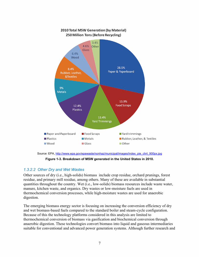
1.3.3 Feedstock Conversion Technologies 1.3.3.1 Combustion Direct combustion is the most common method of producing heat, power, or CHP from MSW resources. In a direct combustion system the MSW is burned to generate heat. The heat is then used to boil water in a boiler, which can be used for heating/cooling applications, process applications, or driving steam turbines to generate electricity. Figure 1-4 shows a diagram of a direct combustion system.

Source: EERE Tribal Energy Program, http://www1.eere.energy.gov/tribalenergy/guide/biomass_biopower.html

Figure 1-4. Direct combustion system. The two principal types of direct combustion boiler systems that utilize MSW are fixed-bed (stationary grate, traveling grate, stoker) and fluidized-bed systems. In a fixed-bed system, the MSW is fed onto a grate where it combusts as air passes through the fuel, releasing the hot flue gases into the heat-exchanger section of the boiler to generate steam. In modular mass-burn systems, there is a secondary chamber where the off-gases from combustion are more fully combusted for heat generation prior to passing into the waste heat boiler stage. In a fluidized-bed system, the biomass is fed into a hot bed of suspended, incombustible particles (such as sand), where the biomass combusts to release the hot flue gas. Fluidized-bed systems are said to produce more complete combustion of the feedstock, resulting in reduced emissions and improved system efficiency. Compared to fixed-bed systems, fluidized-bed boilers also can utilize a wider range of feedstocks.

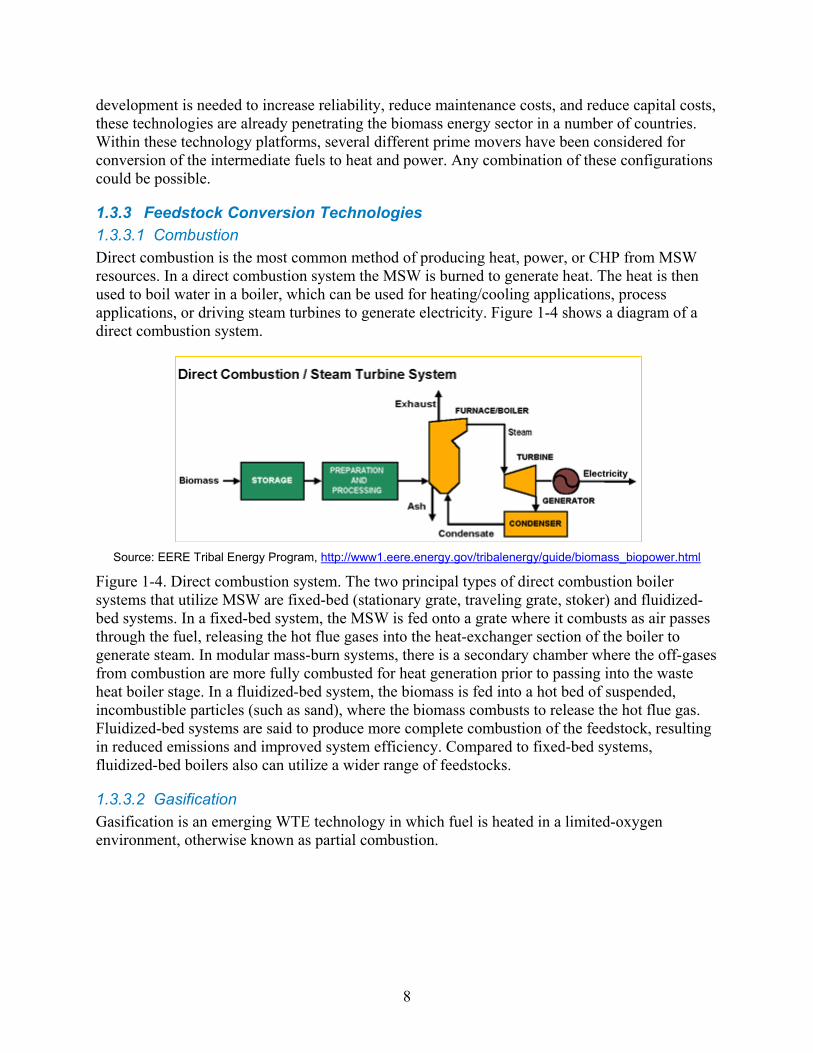
1.3.3.2 Gasification Gasification is an emerging WTE technology in which fuel is heated in a limited-oxygen environment, otherwise known as partial combustion.

9

Figure 1-5. McNeil Generating Station in Burlington, Vermont, uses gasification technology to

convert wood chips to power. Photo by Warren Gretz, NREL/PIX 04734

Gasification is a high-temperature process that is optimized to produce a fuel gas from dry biomass with a minimum of liquids and solids. Gasification consists of heating the feed material in a vessel with partial addition of oxygen or air. Water might or might not be added. Thermochemical reactions take place, and a mixture of hydrogen and carbon monoxide (CO) are the predominant gas products, along with water, methane, carbon dioxide (CO2), nitrogen (if air is used), and other hydrocarbons such as C2H2, C2H4, and C2H6. The resultant gas is called variously producer gas or syngas (synthetic natural gas).

1.3.3.3 Pyrolysis Pyrolysis is a high-temperature process that is optimized to produce pyrolysis oils, bio-char, and synthesis gas from dry biomass. Pyrolysis consists of heating the feed material in a vessel without the addition of oxygen. Decomposition reactions take place, and a mixture of hydrogen and CO are the predominant gas products. Other products include pyrolysis oil, water, methane, and CO2. The resultant gas is called variously biogas, producer gas, or syngas (synthetic natural gas). The composition of the resultant fuels is determined by a combination of the initial mixture of feedstock constituents, temperature, and time within the reactor.

1.3.3.4 Anaerobic Digestion Anaerobic digestion is a biochemical process in which microorganisms break down biodegradable MSW in the absence of oxygen (or air) into methane and carbon dioxide, otherwise known as biogas. This is also the principal process occurring in the decomposition of food wastes and other biomass in landfills. Anaerobic digestion feedstocks are primarily sewage sludge, agricultural and industrial wastes, and other high-moisture-content wastes. The biogas

10

produced can be used directly for heating, CHP gas engines, or upgraded to pipeline-quality gas called biomethane or renewable natural gas.

1.4 Methods for Energy Recovery 1.4.1 Heat Recovery 1.4.1.1 Solid Fuels Traditional WTE facilities utilize solid fuel combustion techniques, which include combusting the feedstock within a furnace and recovering the heat within a traditional boiler or a heat-recovery steam generator (HRSG). Boiler efficiencies for conventional combustion and heat recovery can reach 91%; typically, the larger the unit, the higher the pressure and temperature, the more efficient. Total plant heat rates for solid fuel systems, including WTE systems, are typically 14,000 to 16,000 Btu/kWh. The larger the plant size is, the lower the plant heat rate. The boiler recovers heat from the combustion of the feedstock in the form of steam.

Boiler design is dependent on the quality of the feedstock and the intended use for the steam. Boilers designed for thermal load only are typically low-pressure units in the range of 150 psig to 600 psig. Boilers designed for power generation for a WTE facility are often designed for pressures upward of 1,200 psig. Depending on the constituents within the feedstock, the design pressure can be limited due to acid gas corrosion. When chlorides are present, larger boilers are limited to 850 psig due to the temperature profile across the super heater tubes. Also, in the presence of chlorides, more expensive materials are mandatory.

1.4.1.2 Synthesis Gas Synthesis gas or syngas is a fuel generated through gasification or pyrolysis of a feedstock, and consists of primarily CO2, CO, hydrogen, and possibly methane. During the conversion process from feedstock to syngas, other byproducts are formed, including acid gases (SOx and HCl), tars, and biochar. These byproducts can be addressed through quenching, the use of catalysts to crack the tars, and scrubbing for the removal of acid gases prior to use within a packaged boiler. Alternatively, the fuel can be burned within a furnace or thermal oxidizer to generate heat. The heat then is recovered through an HRSG in the form of steam. An HRSG can have a thermal efficiency of about 92%.

Heat-recovery steam generator design is also dependent on the quality of the feedstock. Those designed for thermal load only are typically low-pressure units sized in the range of 150 psig to 600 psig. Those designed for power generation for a WTE facility are often designed for pressures upward of 1,200 psig. Depending on the constituents within the feedstock, the design pressure can be limited due to acid gas corrosion.

1.4.2 Power Generation Steam generated through direct combustion, close-coupled gasification, close-coupled pyrolysis, or biogas combustion can be utilized in a Rankine steam cycle (RSC) to generate electricity. The process includes the generation of steam at a set pressure, then adding additional heat to produce a superheated steam. The superheated steam is expanded through a steam turbine to convert the thermal energy to mechanical energy, which turns a generator. The generator generates electricity when spinning. Rankine cycle efficiencies are limited to the ideal efficiency, which is defined by the ratio of the energy out to the total energy put into the system. A typical RSC is

11

26% to 30% efficient. Typically, the higher pressure the system, the more efficient the system. This efficiency range provides economics for utilities to utilize the RSC for power generation.

1.4.3 Pipeline Injection Biogas from anaerobic digestion food wastes and other high-moisture MSW can be upgraded to pipeline-quality for use as a renewable natural gas. This upgraded gas may be used as a replacement for natural gas for combined-cycle power plants, for heating, and as a vehicle fuel.

1.5 Renewable Energy Optimization WTE Analysis Module The WTE module delivers performance data based on user inputs. The module can be used as a standalone utility or integrated into REO. It can utilize a combination of user inputs and REO optimizer inputs to quickly predict performance expected from a heat plant, power generation facility, or a CHP plant. The user inputs are shown in Figure 1-6. User inputs include tons of available feedstock, monthly electricity and heat use and cost, and the MSW tipping fee. The user also inputs economic factors such as inflation, energy escalation, and discount rates. For federal analysis, these rates are proscribed by the National Institute of Standards and Technology (NIST). For many inputs, a default value commonly used for WTE facilities is also provided, and can be changed by the user.

Item Units REO Data DefaultAvailable Feedstock Ton/month 15,000 3000Monthly Electricity Consumed kW-hrs 20,000 2000Monthly Heat Consumed MMBtu's 3,000,000 1000

Item Units User Input DefaultCapacity factor % 85% 85%Tip Fee $/Ton 30$ 30.00$ Cost on Electricity $/kw-hr 0.1068$ 0.10$ Cost on Heat $/MMBtu 34.0500$ 7.00$ HHV Waste Btu/lb 5,000 5000Labor Fringe % % 35% 35%

Item Units User Input Private Ownership Default

Gov Ownership Default

Leverage % 0% 0% 0%Interest Rate % 4.0% 4.0% 4.0%Term years 20 20 20Investment Tax Credit (1-yes, 0-no) 0 0 0%Escalation % 4%

User Input Private Ownership Default

Parasitic Load % 5% 5%Recovered Materials %-lbs 10.0% 0.0%Ash Residue %-lbs. 25% 25%

Import/Input Data

User Interface Data

Capitalization

Performance

Figure 1-6. User input.

12

The user also determines whether the tool is calculating performance and economics for power generation only, heat generation only, or CHP.

The WTE module provides an estimation of fixed and variable operation and maintenance expenses, determined by final facility size and technology (heat, power, CHP, etc.). The outputs of the model include boiler size, power generation based on monthly thermal demand, heat generation capacity, and excess energy being utilized to generate electricity. A CHP total net efficiency is also determined on a monthly basis.

1.5.1 Calculation of Electrical Load Met by WTE User inputs for monthly electricity demand are utilized to determine anticipated maximum power generation efficiency. The maximum power generation efficiency is calculated for a power generation steam cycle, based on a 750 psig steam cycle. To determine power generation efficiencies, Thermoflow – Steam Pro heat balance software was used to create generic heat balances for 1 MW net through 100 MW net RSC systems, and a curve fit for the overall net power generation efficiencies versus power output was generated. Figure 1-7 below provides the performance basis for WTE from 1 MW to 100 MW of electric power generation capacity.

Figure 1-7. Electrical efficiency (net) % vs. kW.

Once the power generation capacity and power generation efficiency are determined, the efficiency is used to determine the total heat input required to meet this demand.

1.5.2 Calculation of Thermal Load Met by WTE The WTE module calculates the thermal load based on maximum monthly heat loads and power generation. The thermal load is used to determine boiler output sizing based on MMBtu/hr sizing. Upon determining the boiler output requirements for thermal loads, the module utilizes a sizing curve to identify the boiler efficiency from an efficiency curve developed based on typical boiler efficiencies versus size.

y = 0.0212ln(x) + 0.0281 R² = 0.9707

0%

5%

10%

15%

20%

25%

30%

0 20000 40000 60000 80000 100000 120000

Turbine Efficiency (Net) %

Log. (Turbine Efficiency (Net) %)

13

Figure 1-8. Boiler efficiency (net) percentage vs. boiler output (MMBtu).

1.5.3 Calculation for CHP The WTE module utilizes initial use inputs to determine if a CHP facility is to be considered. In the event there is both heat and electric power demand, the module utilizes the electricity generation net efficiency and boiler net efficiency to determine a CHP performance curve. The curve locates the net power generation efficiency on the Y-axis and the net boiler efficiency on the X-axis. A linear curve from the power generation efficiency to the net power efficiency is generated. This curve identifies the performance of the CHP facility based on the quantity of the total heat introduced into the system. The corresponding percent of the heat input is allocated to heat and to power production. The CHP efficiency is the sum of the net turbine efficiency and net boiler efficiency, as determined by the performance curve shown in Figure 1-9. When the system has no heat demand, and 100% of the heat is used for power generation, the quantity of electricity generated is determined by multiplying the total heat input by the net electrical generation efficiency, which is determined at the left side of the curve (0% heat demand). When the demand is for 100% heat, and no power generation, the quantity of heat generated is determined at the far right of the curve (0% electric generation). When the system requires a portion of the total heat input for heat and a portion for electricity, the corresponding electric and heat generation efficiencies from the middle of the curve are utilized.

To determine the CHP efficiency of the facility, simply adding the net electrical efficiency and the net heat generation efficiency determines the total CHP efficiency.

y = 0.0186ln(x) + 0.7659 R² = 0.3231

76%

78%

80%

82%

84%

86%

88%

90%

92%

0 200 400 600 800 1000 1200

Boiler Efficiency (Net) %

Log. (Boiler Efficiency (Net)%)

14

Figure 1-9. CHP performance: net electrical efficiency vs. net boiler efficiency.

1.5.4 Calculation of WTE Consumption The WTE module determines the total waste consumption based on demand and system-predicted efficiencies. Dividing the total electrical and thermal demand by the CHP efficiency, determined above, the total fuel heat input (in MMBtu/hr) will be determined. Multiplying the fuel heat input by the “User” input for fuel heating value, a fuel flow rate is determined and presented in the results with units of tons per day (TPD) and tons per hour (TPH).

1.5.5 Annual Fixed and Variable Operations & Maintenance Cost Annual fixed and variable operations and maintenance (O&M) costs are predicted utilizing an estimate of labor requirements, fuel use, water use, and chemical use. Each of the identified items is determined based on fuel heat input and the complexity and type of system (heat generation, power generation, or CHP). Heat generation requires the least amount of labor; CHP would require the largest amount of labor for the same amount of heat input.

1.5.6 Calculation of Capital Cost Capital cost estimates are broken down into five areas: heat generation (thermal only, electrical only, or CHP), power generation, balance of plant, engineering, and construction.

Cost curves for each of the five areas were developed. Costs for boiler systems are based on two cost curves, one for power production/CHP systems and one for heat only. When the system is designed for heat only, the module assumes a 250 psig boiler system and computes the system costs based on heating boiler costs. When any power generation is utilized, the module assumes a typical 750 psig boiler and incorporates the higher material costs into the total equipment costs.

Additional cost curves have been developed for steam turbines, condensers, transformers, and cooling systems.

y = -0.1073x + 0.0988 R² = 1

-2%

0%

2%

4%

6%

8%

10%

12%

0% 20% 40% 60% 80% 100%

Net

Ele

ctric

al G

ener

atio

n Ef

ficie

ncy

Net Boiler Efficiency

CHP PERFORMANCE

Linear (CHPPERFORMANCE)

15

Balance of plant cost curves have been developed to encompass the smaller equipment, including water treatment, buildings, etc.

Construction costs are dependent on plant size. Smaller plant designs are typically packaged equipment, which have relatively low installation costs. Larger systems require more field labor to install, driving up the construction costs.

16

2 Life Cycle Assessments for Municipal Waste Combustion

2.1 Introduction Energy and environmental life cycle assessments (LCAs) attempt to estimate the impacts of products and services across all their life stages, from raw materials to disposal. In the case of waste-to-energy (WTE) facilities, life stages considered may include waste collection and transportation to the WTE plant location, as well as municipal solid waste (MSW) combustion and recycling and disposal of combustion residuals. This project briefly reviews results from previous LCA studies of WTE that have been published in the literature, and then uses an existing LCA inventory tool to perform a screening-level analysis of cost, net energy production, greenhouse gas (GHG), and conventional air pollution emissions impacts of WTE for residual MSW in Boulder, Colorado. Boulder was selected as the case study location due to interest in WTE expressed by city staff members and availability of recent data on residual waste composition. The level of waste diversion for recycling and composting in Boulder is already high, compared to national averages. Boulder diverted 46% of its waste in 20106, compared to a national average of 30%. Consequently, the city provides an interesting opportunity to examine the energy and environmental impacts of combustion of the MSW that remains after implementation of a relatively aggressive waste diversion program.

Psomopoulos et al. (2009) present an overview of the recent status of WTE in the United States. Their review indicates 87 WTE facilities in the United States combust about 26 million metric tons of MSW annually and provide a generating capacity of 2700 MW. While there were no new WTE facilities constructed in the United States between 1996 and 2007, Psomopoulos et al. argue that prospects for adding new WTE capacity are improving, in part due to implementation of tighter air pollution emissions standards. Since 2000, four WTE facilities have been expanded and one new facility approved for construction. Psomopoulos et al. report that based on actual operating data, average electricity production from the existing facilities amounts to about 600 kWh per metric ton of MSW combusted (i.e., about 540 kWh per U.S. short ton MSW). They also indicate that 77% of the existing plants have ferrous metal recovery operations, which together recover more than 700,000 metric tons (about 640,000 short tons) of ferrous material each year.

Cleary (2009) reviewed more than a dozen published LCAs for MSW management, most of which included a thermal treatment alternative. His review focused on methodological issues and indicated that comparison of LCA studies for MSW management is complicated by different choices of system boundaries and by assumptions that are not always completely described. Despite these inconsistencies, Cleary found that the LCA studies generally confirm the “waste hierarchy.” i.e., environmental impacts are lowest for recycling, higher for thermal treatment, and highest for landfill disposal. Cleary presented summary results for acidification potential, global warming potential, and net energy use, which show significant differences across the 6 Lewis, Alisa. “Boulder City Council Study Session, October 11, 2011.” Accessed September 12, 2012: http://www.bouldercolorado.gov/files/City%20Council/Study%20Sessions/2011/2011SS/10112011SS/Update_to_Zero_Waste_Master_Plan_SS_memo_and_attachments.pdf.

17

studies he reviewed. However, it appears that reported estimates of net emissions are often confounded by assumptions about electricity generation that would be displaced by WTE. In contrast, results across studies are much more consistent when direct emissions are compared.

Another source of discrepancy across prior LCA studies of MSW management options is treatment of recycling, with some studies setting up recycling and WTE as separate and competing alternatives (e.g., Morris 2005). However, best current practices as well as other formal studies demonstrate that in well-designed MSW management systems, use of WTE can be compatible with significant upfront recycling and on-site materials recovery (Psomopoulos et al. 2009).

Consonni et al. (2005a; 2005b) compared costs and LCA impacts of alternative WTE methods, including grate combustion with and without prior mechanical treatment, and combustion of refuse-derived-fuel (RDF) in a fluidized-bed combustor. For all options, they assumed thermal treatment was applied after diversion of about 35% of generated waste through selective waste collection. They concluded that neither pre-treatment nor RDF preparation were warranted, as increased costs were not offset by environmental benefits. For grate combustion, they estimated about 590 kWh of electricity could be produced per metric ton of residual MSW (535 kWh per short ton) in small systems (assumed to process 65,000 metric tons per year of residual MSW), with about 810 kWh of electricity produced per metric ton of MSW (735 kWh per short ton) in large systems (assumed to treat 390,000 metric tons per year of residual MSW). The small system would produce about 0.99 kg biogenic CO2 and 0.72 kg fossil CO2 per kWh of electricity as direct emissions from waste combustion (not considering offsets from displaced electricity generating systems). The large system would produce about 0.72 kg biogenic CO2 and 0.53 kg fossil CO2 per kWh of direct emissions. Consonni et al.’s LCA indicates that most CO2 emissions are from waste combustion, rather than plant construction, pollution control reagents and additives, or transport of ash. Estimated costs for WTE treatment in the small system were 124 Euros per metric ton of waste, after sale of electricity at .05 Euros per kWh. Costs were approximately halved for the large system.

Kaplan et al. (2009) compared life-cycle impacts of landfill gas-to-energy and mass-burn WTE for representative conditions in the United States. They estimated about 590 kWh of electricity would be produced per ton of MSW combusted, producing 0.91 kg/kWh of biogenic CO2 and 0.56 kg/kWh of fossil CO2 as direct emissions. Further results from Kaplan et al.’s study are discussed below, for comparison with the Boulder case study results developed here.

2.2 Methods The U.S. EPA (Environmental Protection Agency)-RTI (Research Triangle Institute) International Municipal Solid Waste Decision Support Tool (MSW-DST) was used to conduct the case study for this project. This tool has been in use for more than a decade, and incorporates comprehensive energy, environmental impact, and cost models for MSW management alternatives, including landfill disposal, composting, recycling, and combustion with energy recovery (EPA 2000; Harrison et al. 2000; Kaplan et al. 2009). EPA and RTI have recently been developing a new version of the tool for public distribution (eliminating a previous requirement for use of commercially licensed software). This analysis used a beta version of the new tool that was released to a limited number of users.

18

The MSW-DST is a screening-level tool designed to allow preliminary comparison of costs and energy and environmental impacts of municipal waste management alternatives. The tool includes mass balance accounting of waste flows; process models of waste collection, transfers, diversions for recycling and composting, waste treatment, and disposal; and cost and life-cycle inventory and impact estimates for each process. The LCA considers material and energy savings from avoiding new manufacturing or electricity generation, but does not consider material and energy required for production of capital equipment (e.g., garbage trucks). The MSW-DST operates as a least-cost optimization model for waste management, but also allows specification of diversion targets and constraints so different management options can be explored. Default estimates are provided for all process parameters, but users can replace the default values with site-specific data if they are available.

The Boulder case study scenario included waste generation from detached residences, multifamily residences, and commercial entities. The analysis was limited to consideration of residual wastes after diversion of recycled and compostable material. Construction and demolition wastes were not considered. The case study considers collection and transfer of residual mixed waste, combustion at a WTE facility, and landfill disposal of ash. Due to the lack of detailed information about the landfill where Boulder’s residual MSW is currently discarded, we did not perform new modeling of that waste management alternative. Instead, the results for MSW combustion are compared to estimates of energy and environmental impacts of landfill disposal with electricity generation from landfill gas that Kaplan et al. (2009) developed using a previous version of the MSW-DST model, using nationally representative conditions and assumptions.

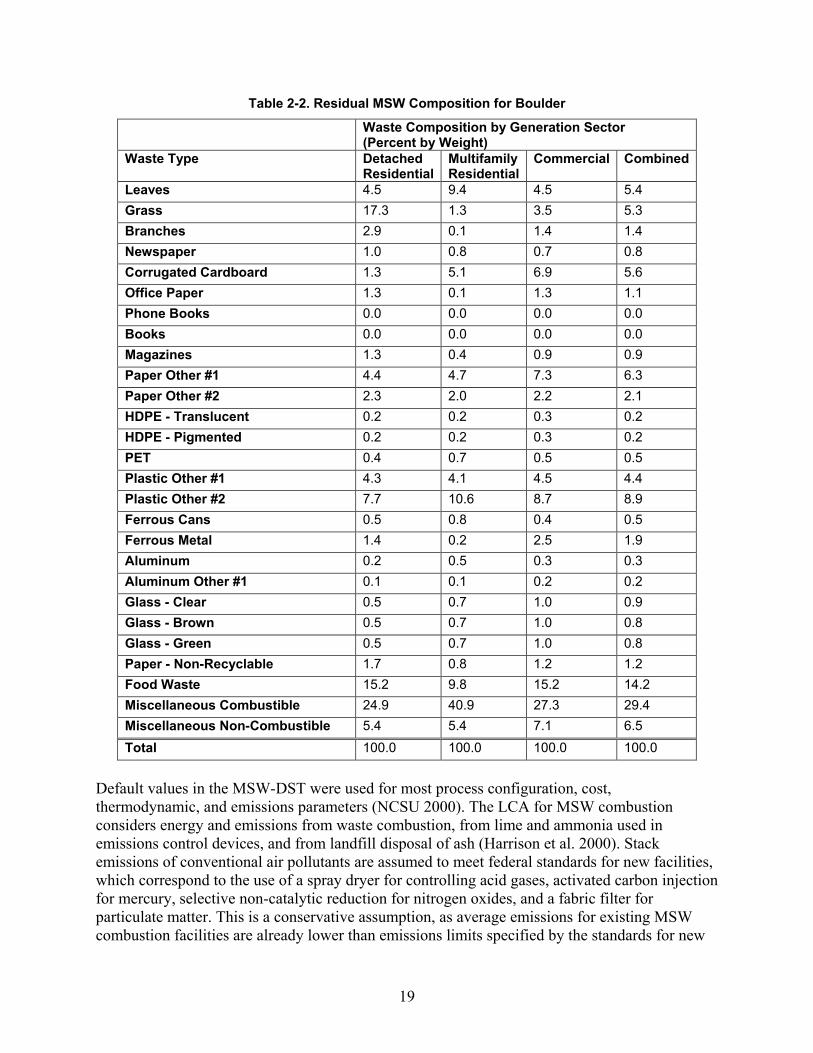
The City of Boulder provided estimates of waste generation rates for this study, which are shown in Table 2-1. (Throughout this and the next section, quantities of MSW and ash are reported in U.S. short tons, as is conventional in the U.S. solid waste management industry.) Waste composition for the city of Boulder was assumed to be the same as that estimated for Boulder County in the County’s 2010 Waste Composition Study (MidAtlantic Consultants, 2010). Their estimates of the composition of residual waste in the detached residential, multifamily residential, and commercial sectors are shown in Table 2. The MSW-DST categories for waste composition from the commercial sector did not include yard waste or food wastes, which respectively comprise over 9% and 15% of commercial waste in Boulder. Waste generated in Boulder’s commercial sector was consequently modeled in the MSW-DST as coming from a second multifamily residential sector, which included categories for yard and food waste.

Table 2-1. Residual MSW Production Rates and Waste Collection Points for Boulder

Detached Residential

Multifamily Residential

Commercial Total

Mass (tons/yr) 12,715 14,558 50,985 78,259 Collection Points 19,425 1,118 2,986 23,529

19

Table 2-2. Residual MSW Composition for Boulder

Waste Composition by Generation Sector (Percent by Weight)

Waste Type Detached Residential

Multifamily Residential

Commercial Combined

Leaves 4.5 9.4 4.5 5.4 Grass 17.3 1.3 3.5 5.3 Branches 2.9 0.1 1.4 1.4 Newspaper 1.0 0.8 0.7 0.8 Corrugated Cardboard 1.3 5.1 6.9 5.6 Office Paper 1.3 0.1 1.3 1.1 Phone Books 0.0 0.0 0.0 0.0 Books 0.0 0.0 0.0 0.0 Magazines 1.3 0.4 0.9 0.9 Paper Other #1 4.4 4.7 7.3 6.3 Paper Other #2 2.3 2.0 2.2 2.1 HDPE - Translucent 0.2 0.2 0.3 0.2 HDPE - Pigmented 0.2 0.2 0.3 0.2 PET 0.4 0.7 0.5 0.5 Plastic Other #1 4.3 4.1 4.5 4.4 Plastic Other #2 7.7 10.6 8.7 8.9 Ferrous Cans 0.5 0.8 0.4 0.5 Ferrous Metal 1.4 0.2 2.5 1.9 Aluminum 0.2 0.5 0.3 0.3 Aluminum Other #1 0.1 0.1 0.2 0.2 Glass - Clear 0.5 0.7 1.0 0.9 Glass - Brown 0.5 0.7 1.0 0.8 Glass - Green 0.5 0.7 1.0 0.8 Paper - Non-Recyclable 1.7 0.8 1.2 1.2 Food Waste 15.2 9.8 15.2 14.2 Miscellaneous Combustible 24.9 40.9 27.3 29.4 Miscellaneous Non-Combustible 5.4 5.4 7.1 6.5 Total 100.0 100.0 100.0 100.0

Default values in the MSW-DST were used for most process configuration, cost, thermodynamic, and emissions parameters (NCSU 2000). The LCA for MSW combustion considers energy and emissions from waste combustion, from lime and ammonia used in emissions control devices, and from landfill disposal of ash (Harrison et al. 2000). Stack emissions of conventional air pollutants are assumed to meet federal standards for new facilities, which correspond to the use of a spray dryer for controlling acid gases, activated carbon injection for mercury, selective non-catalytic reduction for nitrogen oxides, and a fabric filter for particulate matter. This is a conservative assumption, as average emissions for existing MSW combustion facilities are already lower than emissions limits specified by the standards for new

20

facilities (Kaplan et al. 2009). Emissions of biogenic and fossil carbon dioxide are determined based on the input composition of MSW. Ash generation is determined based on the non-combustible fraction of MSW along with the fraction of combustible MSW that remains unburned due to incomplete combustion. Electricity output from the MSW combustion facility is determined based on the quantity, heat, and moisture content of individual MSW components, together with the efficiency of the combustion and electricity generation system. As a base assumption for the analysis, we used a system efficiency of 20% (17,000 Btu/hour).

The LCA reflects emissions from electricity used in MSW management operations, as well as emissions from transportation fuels. For this analysis, MSW was assumed to be collected from residences and multifamily and commercial collection points by diesel-fueled truck, with transport to a WTE facility located 20 miles away. Electricity used in MSW management operations was assumed to come from the Western Systems Coordinating Council. The MSW-DST uses fuel mix and generating efficiencies for each North American Electric Reliability Council region from the mid-1990s (Dumas, 1999). While this information could be updated for a more refined analysis, this is not an option with the currently available version of the MSW-DST, and in any case it has little influence on the results. To examine the net impacts of generating electricity from MSW, we considered a scenario in which it would displace electricity generation from a coal-fired power plant with an assumed generation efficiency of 32% (Dumas 1999).

The MSW-DST provides screening-level estimates of costs of MSW management alternatives, including collection, transfer, transport, treatment, and disposal stages of MSW operations. Costs for the MSW combustion system include annualized capital costs and operations and maintenance (O&M) costs for the combustion facility, less revenues from the sale of ferrous material recovered from incoming MSW and bottom ash, and from the sale of electricity. We used default estimates from the MSW-DST of $310 per design ton per year for capital costs and $65 per design ton per year for O&M. The cost estimates used in the MSW-DST were derived from estimates EPA made for four model WTE plants in preparation for setting emissions standards (EPA 1989), updated to current dollars. We assumed a plant life of 30 years (increased from the default assumption of 20 years), plant capacity factor of 0.91, and discount rate of 5% for capital recovery. We also assumed electricity could be sold for $.04/kWh and scrap iron for $350 per ton7. There may be additional revenue potential from selling renewable energy credits (RECs), but this is not included in this analysis.

2.3 Results As shown in Table 2-3, the MSW-DST tool estimates that 78,300 tons of residual MSW collected in Boulder each year (215 tons per day (TPD)8) could be used to generate about 45 million kWh of electricity. This generation rate corresponds to the output from about a 5.6 MW capacity power plant, assuming a 91% capacity factor. The MSW-DST tool estimates 12,000 tons of ash would be produced in the combustion process. Direct air emissions from MSW

7 Based on estimated $0.175/pound from http://www.metalprices.com/p/SteelScrapIronFreeChart/. Accessed September 12, 2012. 8 215 TPD is low compared to the national average WTE size of ~1,000 TPD for mass burn waterwall technology. A modular or small mixed-waste processing facility with fluidized-bed technology should be considered in future research.

21

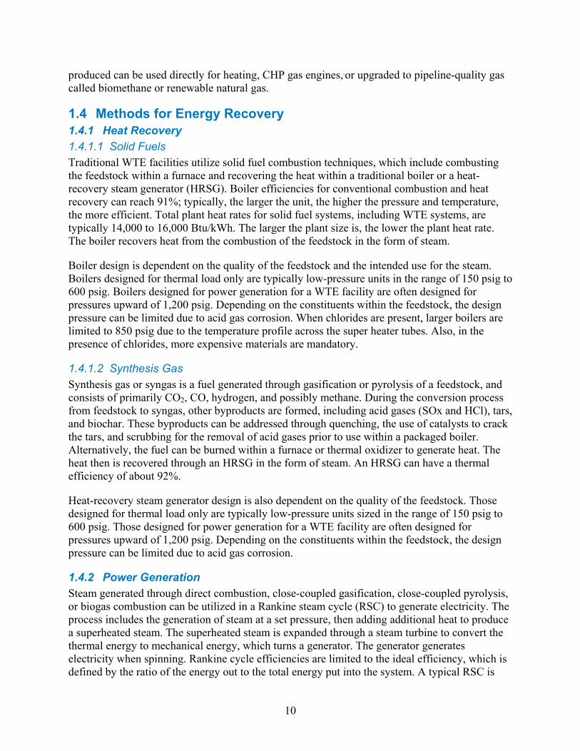
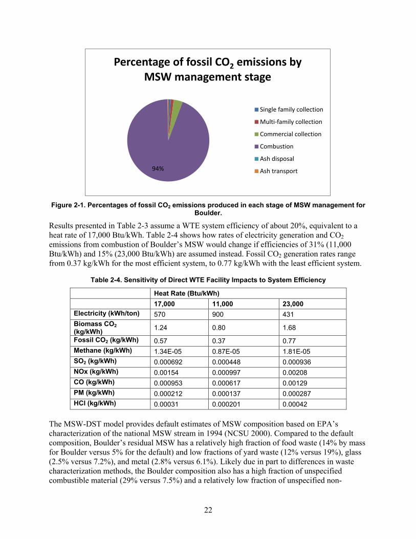
combustion, assuming a facility that just meets federal air quality standards, include an estimated 69,000 kg/year of nitrogen oxides (NOx), 31,000 kg/year of silicon dioxide (SO2), and 9,500 kg/year of particulate matter (PM). In addition, the MSW-DST tool estimates that MSW combustion would produce 55.5 million kg/year of biomass CO2 and 25.6 million kg/year of fossil CO2. As shown in Figure 2-1, the MSW-DST tool indicates these MSW combustion emissions of fossil CO2 dominate those from other stages in the MSW management process.

The MSW-DST tool provides rough estimates of annualized system costs, including costs for waste combustion and ash disposal and assuming sales of electricity at $.04/kWh and scrap iron at $350/ton. The resulting annualized costs for treating Boulder’s 78,300 tons of residual MSW using WTE are about $4.5 million, or $58/ton (excluding costs of collection and waste transport to the facility).

If electricity from combustion of Boulder’s residual MSW is viewed as displacing electricity from a typical coal-fired power plant, nearly 50 million kg of fossil CO2 from coal combustion would be displaced. Thus, comparing fossil CO2 emissions from MSW combustion (including emissions associated with ash disposal) with CO2 emissions from coal combustion, switching to MSW could reduce fossil CO2 emissions by about 25 million kg/year. Based on MSW-DST estimates, the switch could also reduce methane emissions by about 60,000 kg/year.

Table 2-3. Estimated Impacts of Combustion Stage of WTE for Boulder MSW

WTE Facility

WTE with Ash Transport and Disposal (Direct)

Displacement from Coal-Fired Generation

WTE with Ash Disposal Displacing Coal but No Metals Recovery

WTE with Ash Disposal and Ferrous Metals Recovery Displacing Coal

Waste Combustion (tons/year)

78,300

Ash Disposal (tons/year)

12,000

Electricity Production (kWh/year)

44,800,000 44,800,000 44,800,000 0 0

Coal Energy (MMBtu/year)

498,000 -496,000 -515,000

Biomass CO2 (kg/year)

55,500,000 55,500,000 3200 55,500,000 55,500,000

Fossil CO2 (kg/year)

25,600,000 25,600,000 48,600,000 -23,000,000 -24,500,000

Methane (kg/year) 600 600 58,000 -57,300 -58,600 SO2 (kg/year) 31,000 31,200 329,000 -298,000 -300,310 NOx (kg/year) 69,000 69,800 139,000 -69,600 -70,900 CO (kg/year) 42,700 43,300 8,600 34,700 16,200 PM (kg/year) 9,500 9,600 37,400 -27,800 -35,400 HCl (kg/year) 13,900 13,900 12,800 1,000 1,050

22

Figure 2-1. Percentages of fossil CO2 emissions produced in each stage of MSW management for

Boulder.

Results presented in Table 2-3 assume a WTE system efficiency of about 20%, equivalent to a heat rate of 17,000 Btu/kWh. Table 2-4 shows how rates of electricity generation and CO2 emissions from combustion of Boulder’s MSW would change if efficiencies of 31% (11,000 Btu/kWh) and 15% (23,000 Btu/kWh) are assumed instead. Fossil CO2 generation rates range from 0.37 kg/kWh for the most efficient system, to 0.77 kg/kWh with the least efficient system.

Table 2-4. Sensitivity of Direct WTE Facility Impacts to System Efficiency

Heat Rate (Btu/kWh) 17,000 11,000 23,000 Electricity (kWh/ton) 570 900 431 Biomass CO2 (kg/kWh) 1.24 0.80 1.68

Fossil CO2 (kg/kWh) 0.57 0.37 0.77 Methane (kg/kWh) 1.34E-05 0.87E-05 1.81E-05 SO2 (kg/kWh) 0.000692 0.000448 0.000936 NOx (kg/kWh) 0.00154 0.000997 0.00208 CO (kg/kWh) 0.000953 0.000617 0.00129 PM (kg/kWh) 0.000212 0.000137 0.000287 HCl (kg/kWh) 0.00031 0.000201 0.00042

The MSW-DST model provides default estimates of MSW composition based on EPA’s characterization of the national MSW stream in 1994 (NCSU 2000). Compared to the default composition, Boulder’s residual MSW has a relatively high fraction of food waste (14% by mass for Boulder versus 5% for the default) and low fractions of yard waste (12% versus 19%), glass (2.5% versus 7.2%), and metal (2.8% versus 6.1%). Likely due in part to differences in waste characterization methods, the Boulder composition also has a high fraction of unspecified combustible material (29% versus 7.5%) and a relatively low fraction of unspecified non-

94%

Percentage of fossil CO2 emissions by MSW management stage

Single family collection

Multi-family collection

Commercial collection

Combustion

Ash disposal

Ash transport

23

combustible material (6.5% versus 12.3%). The relative amounts of plastic and paper in the two waste profiles are similar. Table 2-5 shows that these differences in composition have only a modest influence on most impacts from MSW combustion. We estimate that Boulder residual MSW would produce about 4% more electricity per ton of waste than expected based on the default composition. For most pollutants, emissions per kWh of electricity produced are about 10% higher with Boulder’s waste composition than with the default composition. On the other hand, with Boulder’s residual MSW composition, ash generation per ton of waste is estimated to be about half that expected based on the default composition. The lower rate of ash production is due to lower fractions of glass, metal, and miscellaneous non-combustible waste in Boulder’s residual MSW.

Table 2-5. Comparison of WTE Combustion Stage Impacts for Boulder MSW with Impacts for National Default Residential MSW

Boulder MSW

Default Residential MSW

Electricity (kWh/ton) 570 550 Biomass CO2 (kg/kWh) 1.24 1.09 Fossil CO2 (kg/kWh) 0.57 0.52 Methane (kg/kWh) 1.34E-05 1.39E-05 SO2 (kg/kWh) 0.000692 .000623 NOx (kg/kWh) 0.00154 .00139 CO (kg/kWh) 0.000953 .000859 PM (kg/kWh) 0.000212 .000195 HCl (kg/kWh) 0.00031 .000273

Comparisons of impacts of MSW combustion with land disposal and energy recovery from landfill gas are highly uncertain, due to uncertainty in rates of landfill gas generation and gas capture efficiencies. Furthermore, we lacked detailed information on landfill configuration and operations for Boulder. In the absence of site-specific data and other information necessary to make more precise estimates, Table 2-6 provides a rough comparison of emissions rates for combustion of Boulder residual MSW with published estimates for landfill gas with energy recovery (Kaplan et al. 2009), which were also developed using the MSW-DST model and are meant to represent typical conditions in the United States. Table 2-7 shows the corresponding total impacts estimated for disposal of 78,300 tons per year of residual MSW. The emissions comparisons in Tables 2-6 and 2-7 are made for direct emissions, without factoring in any credit for displaced electricity generation from other sources.

The comparisons in Tables 2-6 and 2-7 suggest that MSW combustion can produce about nine times more electricity per ton of waste than energy recovery from landfill gas. Compared to energy recovery from landfill gas, MSW combustion is estimated to produce about half the biomass CO2 per kWh electricity, and about five times as much fossil CO2 per kWh. However, energy recovery from landfill gas is estimated to release much larger quantities of methane into the atmosphere compared to MSW combustion. Combining fossil CO2 and methane emissions and using a global warming potential of 21 for methane, the CO2-equivalent emissions rate for landfill gas with energy recovery is about five times that for WTE, per unit electricity generated.

24

In terms of absolute emissions, Table 2-7 suggests that landfill disposal of Boulder’s residual MSW would produce a little less than 60% of the CO2-equivalent GHGs and substantially less conventional air pollution (SO2, NOx, CO, PM, and HCl) than would combustion of the MSW in a facility that just meets national emissions standards9.

Table 2-6. Comparison of Emissions Rates for WTE with Ash Disposal vs. Landfill Gas-to-Energy

Landfill with Energy Recovery*

WTE with Ash Transport and Disposal (Direct)

Electricity Production (kWh/ton)

66.5

570

Biomass CO2 (kg/kWh) 2.4 1.24 Fossil CO2 (kg/kWh) 0.10 0.57 Methane (kg/kWh) 0.13 1.34E-5 CO2 equivalent of fossil CO2 & methane (kg/kWh)

2.8 0.57

SO2 (kg/kWh) 0.00055

0.000696

NOx (kg/kWh) 0.0022

0.00156

CO (kg/kWh) 0.0038

0.000966

PM (kg/kWh) 0.00039 0.000215 HCl (kg/kWh) 0.000034 0.00031

* Estimated from emissions factors given in Kaplan et al. (2009) for “LF-VENT2-ICE30” case assuming nationally representative MSW composition with 30-year energy recovery from landfill gas using internal combustion engine, followed by gas venting for the remaining life of the landfill.

9 Note that using national emission standards penalizes WTE technology. Average emission performance for WTE plants is typically 10%–20% of the standard for most GHGs, except NOx, which is 50%–90% of the standard.

25

Table 2-7. Comparison of Estimated Impacts of WTE vs. Landfill Disposal for Boulder MSW

Landfill Disposal with Energy Recovery*

WTE with Ash Transport and Disposal (Direct)

Electricity Production (kWh/year)

5,200,000

44,800,000

Biomass CO2 (kg/year) 12,500,000 55,500,000 Fossil CO2 (kg/year) 520,000 25,600,000 Methane (kg/year) 677,000 600 CO2 equivalent of fossil CO2 & methane

14,700,000 25,600,000

SO2 (kg/year) 2860

31,200

NOx (kg/year) 11,600

69,800

CO (kg/year) 19,900

43,300

PM (kg/year) 2040 9600 HCl (kg/year) 177 13,900

* Estimated from emissions factors given in Kaplan et al. (2009) for case assuming nationally representative MSW composition with 30-year energy recovery from landfill gas using internal combustion engine, followed by gas venting for the remaining life of the landfill. 2.4 Conclusions The analysis presented in this study is meant to be a first-order screening analysis, and as such relies on many default assumptions that were developed by EPA and RTI to represent typical conditions nationally, not site-specific conditions for Boulder. Cost estimates for WTE are based on an EPA study conducted more than 20 years ago and thus do not reflect advances in technology that have occurred since that time. Air emissions estimates for conventional pollutants are likely to be conservative, as they were developed assuming the WTE facility would just meet federal air quality standards.

Life cycle assessment studies published in the literature have generally been consistent in suggesting that MSW combustion is a better alternative to landfill disposal in terms of net energy impacts and CO2-equivalent GHG emissions. The results from this study match that expectation. In this report, WTE leads to a higher reduction in emissions compared to landfill-to-energy disposal per kWh production. The screening cost estimates provided by the MSW-DST indicate WTE would be a relatively expensive way to treat Boulder’s residual MSW, at an estimated cost of about $58 per ton after accounting for sales of electricity and ferrous metal. This is higher than typical landfill costs for this region (Arsova et al. 2008).

If electricity produced from combustion of Boulder’s residual MSW were to displace coal combustion, fossil CO2 emissions could be decreased by about 20–25 million kg/year. Emissions of SO2, NOx, and PM could also be reduced compared to life-cycle emissions associated with coal combustion. Electricity generation rates and emissions associated with combustion of

26

Boulder’s residual MSW are not sharply different from those estimated assuming a national average MSW composition, despite Boulder’s relatively aggressive recycling and composting programs.

References Arsova, L.; van Haaren, R.; Goldstein, N.; Kaufman, S.; Themelis, N. (2008). “The State of Garbage in America.” Biocycle (49:12); p. 22: http://www.jgpress.com/archives/_free/001782.html.

Cleary, J. (2009). “Life Cycle Assessments of Municipal Solid Waste Management Systems: A Comparative Analysis of Selected Peer-Reviewed Literature.” Environ. Int. (35:8); pp. 1256-1266.

Consonni, S.; Giugliano, M.; Grosso, M. (2005a). “Alternative strategies for energy recovery from municipal solid waste Part A: Mass and energy balances.” Waste Management (25:2); pp. 123-135.

Consonni, S.; Giugliano, M.; Grosso, M. (2005b). “Alternative strategies for energy recovery from municipal solid waste Part B: Emission and cost estimates.” Waste Management (25:2); pp. 137-148.

Dumas, R.D. (1999). Energy Usage and Emissions Associated with Electric Energy Consumption as Part of a Solid Waste Management Life Cycle Inventory Model, Revision 2. Department of Civil Engineering, North Carolina State University, June 1999.

EPA (1989). Municipal Waste Combustors – Background Information for Proposed Standards: 111(B) Model Plant Description and Cost Report, Final Report. U.S. Environmental Protection Agency (EPA).

EPA (2000). A Decision Support Tool for Assessing the Cost and Environmental Burdens of Integrated Municipal Solid Waste Management Strategies: User’s Manual. U.S. Environmental Protection Agency (EPA), Office of Research and Development (ORD).

Harrison, K.W.; Dumas, R.D.; Barlaz, M.A.; Nishtala, S.R. (2000). “A life-cycle inventory model of municipal solid waste combustion.” J. Air & Waste Manage. Assoc. (50:6); pp. 993-1003.

Kaplan, P.O.; Decarolis, J.; Thorneloe, S. (2009). “Is it Better to Burn or Bury Waste for Clean Electricity Generation?” Environ. Sci. Technol. (43:6); pp. 1711-1717.

MidAtlantic Solid Waste Consultants (2010). Boulder County Waste Composition Study.

Morris, J. (2005). “Comparative LCAs for Curbside Recycling Versus Either Landfilling or Incineration with Energy Recovery.” Int. J. LCA (10:4); pp. 273-284.

NCSU (2000). Default Data and Data Input Requirements for the Municipal Solid Waste Management Decision Support Tool. North Carolina State University and Research Triangle Institute, December 2000.

27

Psomopoulos, C.S.; Bourka, A.; Themelis, N.J. (2009). “Waste-to-energy: a review of the status and benefits in USA,” Waste Management (29:5); pp. 1718-1724.

28

3 Air Emissions Limits for Municipal Waste Combustors

As stationary sources of air pollution, municipal waste combustors (MWCs) are subject to multiple provisions of the federal Clean Air Act that lead to construction and operating permit requirements. The two main Clean Air Act provisions leading to emissions limits and/or monitoring and operating practice requirements for MWCs are the specific solid waste combustion provisions in Section 129, and the general “New Source Review” provisions contained in Section 165 for new or modified facilities that would be located in areas that meet the National Ambient Air Quality Standards (NAAQS), and in Section 173 for new or modified facilities that would be located in nonattainment areas. In effect, Section 129 establishes federal New Source Performance Standards (NSPS), which are emissions limits that apply to all new solid waste combustion facilities across the country, along with state-implemented Emissions Guidelines that represent minimum control requirements for all existing solid waste combustion facilities. The New Source Review (NSR) provisions in Sections 165 and 173 additionally require that when states permit construction or substantial modification of solid waste combustion facilities (and other large stationary sources) they perform a case-by-case review to determine if additional controls are warranted, beyond those needed to meet the NSPS. Individual states may impose additional requirements beyond NSPS and NSR, but they cannot relax the federal rules.

Under Section 129 of the Clean Air Act, as amended in 1990, the U.S. EPA is required to set performance standards to limit emissions from solid waste incineration units. EPA has established these standards for several categories of waste incinerators, including large and small MWCs, hospital/medical/infectious waste incinerators, and commercial/industrial waste incinerators. The regulations for large and small MWCs are of primary relevance for this project.

Section 129 defines municipal waste as “refuse (and refuse-derived fuel) collected from the general public and from residential, commercial, institutional, and industrial sources consisting of paper, wood, yard wastes, food wastes, plastics, leather, rubber, and other combustible materials and non-combustible materials such as metal, glass and rock …” (42 U.S.C. §7429(g)). Large municipal waste combustors are defined as those with capacity to combust more than 250 tons of waste per day (42 U.S.C. §7429(a)(1)(C)).

For new units, Section 129 requires emissions standards that reflect the “maximum degree of reduction” in emissions of specified pollutants, with reductions that are at least as stringent as “the emissions control that is achieved in practice by the best controlled similar unit.” For existing units, Section 129 requires standards that are at least as stringent as the “average emissions limitation achieved by the best performing 12 percent of units in the category” (42 U.S.C. §7429(a)(2)). Such emissions limits (which are also prescribed for other categories of hazardous air pollutant sources in Section 112 of the Clean Air Act) are commonly known as maximum achievable control technology (MACT). Standards for new municipal waste combustion units are to be developed and implemented as directly federally enforceable new source performance standards under Section 111(b) of the Clean Air Act, whereas standards for existing units are developed as guidelines under sSection 111(d). The guidelines are implemented and enforced by the states, or by the federal government in the absence of an approved state plan for compliance. The standards are to be reviewed and, if necessary, revised

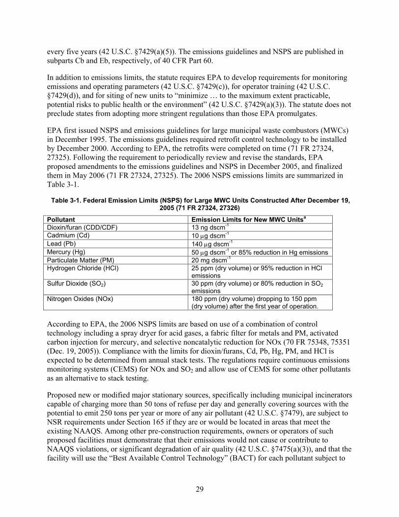
29

every five years (42 U.S.C. §7429(a)(5)). The emissions guidelines and NSPS are published in subparts Cb and Eb, respectively, of 40 CFR Part 60.

In addition to emissions limits, the statute requires EPA to develop requirements for monitoring emissions and operating parameters (42 U.S.C. §7429(c)), for operator training (42 U.S.C. §7429(d)), and for siting of new units to “minimize … to the maximum extent practicable, potential risks to public health or the environment” (42 U.S.C. §7429(a)(3)). The statute does not preclude states from adopting more stringent regulations than those EPA promulgates.

EPA first issued NSPS and emissions guidelines for large municipal waste combustors (MWCs) in December 1995. The emissions guidelines required retrofit control technology to be installed by December 2000. According to EPA, the retrofits were completed on time (71 FR 27324, 27325). Following the requirement to periodically review and revise the standards, EPA proposed amendments to the emissions guidelines and NSPS in December 2005, and finalized them in May 2006 (71 FR 27324, 27325). The 2006 NSPS emissions limits are summarized in Table 3-1.

Table 3-1. Federal Emission Limits (NSPS) for Large MWC Units Constructed After December 19, 2005 (71 FR 27324, 27326)

Pollutant Emission Limits for New MWC Unitsa Dioxin/furan (CDD/CDF) 13 ng dscm-1 Cadmium (Cd) 10 µg dscm-1 Lead (Pb) 140 µg dscm-1 Mercury (Hg) 50 µg dscm-1 or 85% reduction in Hg emissions Particulate Matter (PM) 20 mg dscm-1 Hydrogen Chloride (HCl) 25 ppm (dry volume) or 95% reduction in HCl

emissions Sulfur Dioxide (SO2) 30 ppm (dry volume) or 80% reduction in SO2

emissions Nitrogen Oxides (NOx) 180 ppm (dry volume) dropping to 150 ppm

(dry volume) after the first year of operation. According to EPA, the 2006 NSPS limits are based on use of a combination of control technology including a spray dryer for acid gases, a fabric filter for metals and PM, activated carbon injection for mercury, and selective noncatalytic reduction for NOx (70 FR 75348, 75351 (Dec. 19, 2005)). Compliance with the limits for dioxin/furans, Cd, Pb, Hg, PM, and HCl is expected to be determined from annual stack tests. The regulations require continuous emissions monitoring systems (CEMS) for NOx and SO2 and allow use of CEMS for some other pollutants as an alternative to stack testing.

Proposed new or modified major stationary sources, specifically including municipal incinerators capable of charging more than 50 tons of refuse per day and generally covering sources with the potential to emit 250 tons per year or more of any air pollutant (42 U.S.C. §7479), are subject to NSR requirements under Section 165 if they are or would be located in areas that meet the existing NAAQS. Among other pre-construction requirements, owners or operators of such proposed facilities must demonstrate that their emissions would not cause or contribute to NAAQS violations, or significant degradation of air quality (42 U.S.C. §7475(a)(3)), and that the facility will use the “Best Available Control Technology” (BACT) for each pollutant subject to

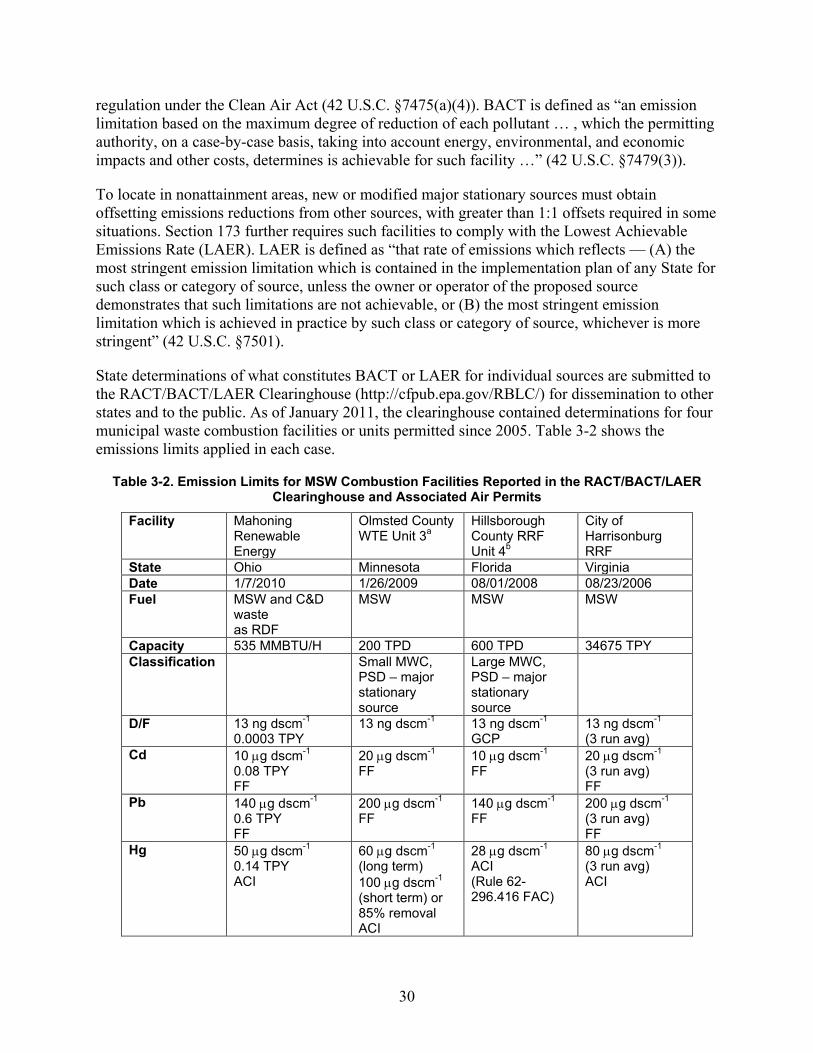
30

regulation under the Clean Air Act (42 U.S.C. §7475(a)(4)). BACT is defined as “an emission limitation based on the maximum degree of reduction of each pollutant … , which the permitting authority, on a case-by-case basis, taking into account energy, environmental, and economic impacts and other costs, determines is achievable for such facility …” (42 U.S.C. §7479(3)).

To locate in nonattainment areas, new or modified major stationary sources must obtain offsetting emissions reductions from other sources, with greater than 1:1 offsets required in some situations. Section 173 further requires such facilities to comply with the Lowest Achievable Emissions Rate (LAER). LAER is defined as “that rate of emissions which reflects — (A) the most stringent emission limitation which is contained in the implementation plan of any State for such class or category of source, unless the owner or operator of the proposed source demonstrates that such limitations are not achievable, or (B) the most stringent emission limitation which is achieved in practice by such class or category of source, whichever is more stringent” (42 U.S.C. §7501).

State determinations of what constitutes BACT or LAER for individual sources are submitted to the RACT/BACT/LAER Clearinghouse (http://cfpub.epa.gov/RBLC/) for dissemination to other states and to the public. As of January 2011, the clearinghouse contained determinations for four municipal waste combustion facilities or units permitted since 2005. Table 3-2 shows the emissions limits applied in each case.

Table 3-2. Emission Limits for MSW Combustion Facilities Reported in the RACT/BACT/LAER Clearinghouse and Associated Air Permits

Facility Mahoning Renewable Energy

Olmsted County WTE Unit 3a

Hillsborough County RRF Unit 4b

City of Harrisonburg RRF

State Ohio Minnesota Florida Virginia Date 1/7/2010 1/26/2009 08/01/2008 08/23/2006 Fuel MSW and C&D

waste as RDF

MSW MSW MSW

Capacity 535 MMBTU/H 200 TPD 600 TPD 34675 TPY Classification Small MWC,

PSD – major stationary source

Large MWC, PSD – major stationary source

D/F 13 ng dscm-1

0.0003 TPY 13 ng dscm-1

13 ng dscm-1

GCP 13 ng dscm-1

(3 run avg) Cd 10 µg dscm-1

0.08 TPY FF

20 µg dscm-1

FF 10 µg dscm-1

FF 20 µg dscm-1

(3 run avg) FF

Pb 140 µg dscm-1

0.6 TPY FF

200 µg dscm-1

FF 140 µg dscm-1

FF 200 µg dscm-1

(3 run avg) FF

Hg 50 µg dscm-1 0.14 TPY ACI

60 µg dscm-1

(long term) 100 µg dscm-1

(short term) or 85% removal ACI

28 µg dscm-1

ACI (Rule 62-296.416 FAC)

80 µg dscm-1

(3 run avg) ACI

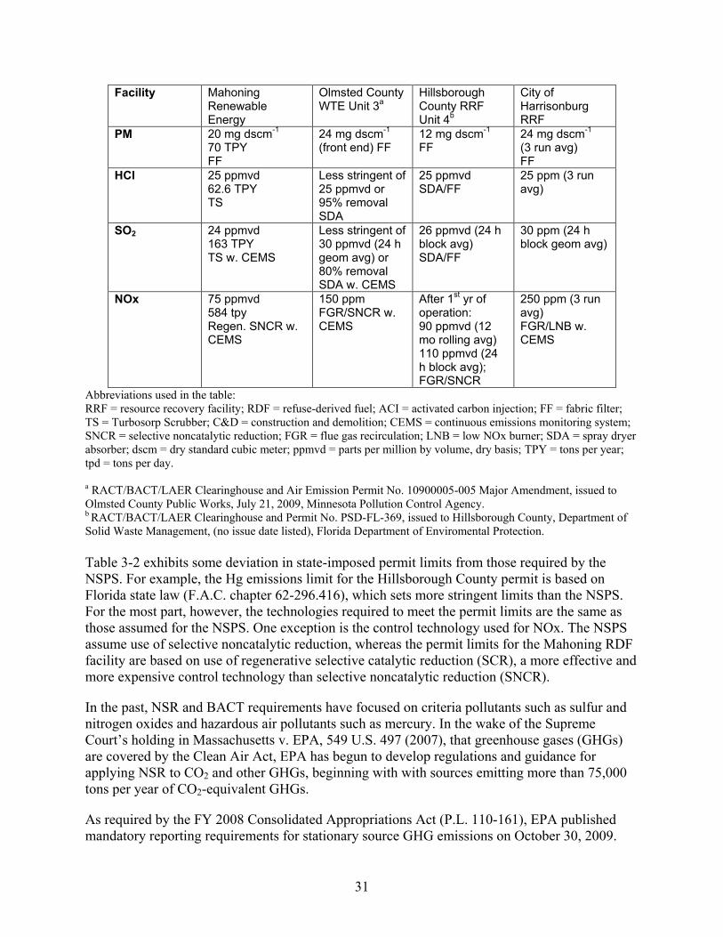
31

Facility Mahoning Renewable Energy

Olmsted County WTE Unit 3a

Hillsborough County RRF Unit 4b

City of Harrisonburg RRF

PM 20 mg dscm-1

70 TPY FF

24 mg dscm-1 (front end) FF

12 mg dscm-1

FF 24 mg dscm-1

(3 run avg) FF

HCl 25 ppmvd 62.6 TPY TS

Less stringent of 25 ppmvd or 95% removal SDA

25 ppmvd SDA/FF

25 ppm (3 run avg)

SO2 24 ppmvd 163 TPY TS w. CEMS

Less stringent of 30 ppmvd (24 h geom avg) or 80% removal SDA w. CEMS

26 ppmvd (24 h block avg) SDA/FF

30 ppm (24 h block geom avg)

NOx 75 ppmvd 584 tpy Regen. SNCR w. CEMS

150 ppm FGR/SNCR w. CEMS

After 1st yr of operation: 90 ppmvd (12 mo rolling avg) 110 ppmvd (24 h block avg); FGR/SNCR

250 ppm (3 run avg) FGR/LNB w. CEMS

Abbreviations used in the table: RRF = resource recovery facility; RDF = refuse-derived fuel; ACI = activated carbon injection; FF = fabric filter; TS = Turbosorp Scrubber; C&D = construction and demolition; CEMS = continuous emissions monitoring system; SNCR = selective noncatalytic reduction; FGR = flue gas recirculation; LNB = low NOx burner; SDA = spray dryer absorber; dscm = dry standard cubic meter; ppmvd = parts per million by volume, dry basis; TPY = tons per year; tpd = tons per day. a RACT/BACT/LAER Clearinghouse and Air Emission Permit No. 10900005-005 Major Amendment, issued to Olmsted County Public Works, July 21, 2009, Minnesota Pollution Control Agency. b RACT/BACT/LAER Clearinghouse and Permit No. PSD-FL-369, issued to Hillsborough County, Department of Solid Waste Management, (no issue date listed), Florida Department of Enviromental Protection. Table 3-2 exhibits some deviation in state-imposed permit limits from those required by the NSPS. For example, the Hg emissions limit for the Hillsborough County permit is based on Florida state law (F.A.C. chapter 62-296.416), which sets more stringent limits than the NSPS. For the most part, however, the technologies required to meet the permit limits are the same as those assumed for the NSPS. One exception is the control technology used for NOx. The NSPS assume use of selective noncatalytic reduction, whereas the permit limits for the Mahoning RDF facility are based on use of regenerative selective catalytic reduction (SCR), a more effective and more expensive control technology than selective noncatalytic reduction (SNCR).

In the past, NSR and BACT requirements have focused on criteria pollutants such as sulfur and nitrogen oxides and hazardous air pollutants such as mercury. In the wake of the Supreme Court’s holding in Massachusetts v. EPA, 549 U.S. 497 (2007), that greenhouse gases (GHGs) are covered by the Clean Air Act, EPA has begun to develop regulations and guidance for applying NSR to CO2 and other GHGs, beginning with with sources emitting more than 75,000 tons per year of CO2-equivalent GHGs.

As required by the FY 2008 Consolidated Appropriations Act (P.L. 110-161), EPA published mandatory reporting requirements for stationary source GHG emissions on October 30, 2009.

32

The rule, which is published in 40 CFR Part 98, utilizes a general reporting threshold of 25,000 metric tons of CO2-equivalent (CO2-e) per year. Municipal solid waste combustion is covered in Subpart C – General Stationary Fuel Combustion Sources. Based on revisions to the original rule published in December 2010 (75 FR 79092), MSW combustion units with capacity to burn more than 600 tons of MSW per day are required to use continuous emissions monitoring systems (CEMS) to measure CO2 emissions (40 CFR 98.33(b)(4)(ii)(A)). Smaller units can report estimated CO2 emissions based on fuel heat content. The biogenic fraction of the CO2 emissions from MSW combustion must be reported separately, based on quarterly sampling and 14C analysis.

In May 2010, EPA issued standards for GHG emissions from light-duty vehicles, making GHGs “regulated pollutants” under the Clean Air Act. This designation triggered further requirements, including the application of stationary source NSR and “Title V” permitting requirements, including application of BACT under the Prevention of Significant Deterioration (PSD) section of the NSR provisions. In order to allow time to implement these requirements for GHG sources, EPA issued the Greenhouse Gas Tailoring Rule on May 13, 2010, restricting the initial applicability of NSR for GHGs to the largest sources, and to sources already subject to NSR or Title V requirements based on non-GHG pollutants. Under the Tailoring Rule, as of July 1, 2011, all new facilities emitting more than 100,000 tons of CO2-e per year and existing facilities that would increase emissions by more than 75,000 tons per year would be subject to PSD and Title V permitting requirements (75 FR 31514, June 3, 2010).

As promulgated, the Tailoring Rule did not clearly distinguish between CO2 emissions from biomass and fossil fuel combustion for determining NSR/Title V applicability. This aspect of the rule was challenged in a petition for reconsideration from the National Alliance of Forest Owners. EPA granted the petition in January 2011. In March 2011, the Agency proposed to defer the application of NSR and Title V permit requirements to biogenic CO2 emissions for three years while it considered options for accounting for these emissions (76 FR 15249, Mar. 21, 2011). The proposed deferral would apply to biogenic CO2 emissions associated with MSW combustion, where EPA defines biogenic CO2 emissions as emissions resulting from decomposition or combustion of non-fossilized and biodegradable organic materials originating from plants, animals, or microorganisms. EPA has not yet finalized the deferral action.

Reference “Clean Air Act.” U.S. Environmental Protection Agency (EPA): http://www.epa.gov/air/caa/.

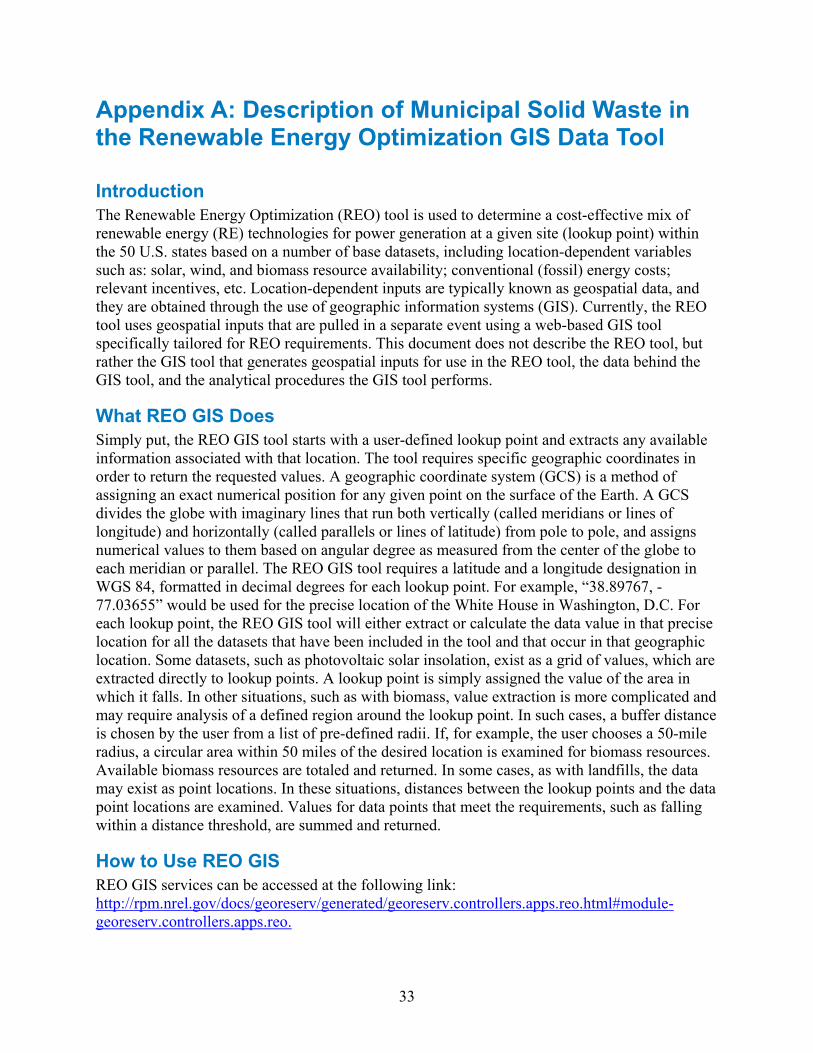
33

Appendix A: Description of Municipal Solid Waste in the Renewable Energy Optimization GIS Data Tool Introduction The Renewable Energy Optimization (REO) tool is used to determine a cost-effective mix of renewable energy (RE) technologies for power generation at a given site (lookup point) within the 50 U.S. states based on a number of base datasets, including location-dependent variables such as: solar, wind, and biomass resource availability; conventional (fossil) energy costs; relevant incentives, etc. Location-dependent inputs are typically known as geospatial data, and they are obtained through the use of geographic information systems (GIS). Currently, the REO tool uses geospatial inputs that are pulled in a separate event using a web-based GIS tool specifically tailored for REO requirements. This document does not describe the REO tool, but rather the GIS tool that generates geospatial inputs for use in the REO tool, the data behind the GIS tool, and the analytical procedures the GIS tool performs.

What REO GIS Does Simply put, the REO GIS tool starts with a user-defined lookup point and extracts any available information associated with that location. The tool requires specific geographic coordinates in order to return the requested values. A geographic coordinate system (GCS) is a method of assigning an exact numerical position for any given point on the surface of the Earth. A GCS divides the globe with imaginary lines that run both vertically (called meridians or lines of longitude) and horizontally (called parallels or lines of latitude) from pole to pole, and assigns numerical values to them based on angular degree as measured from the center of the globe to each meridian or parallel. The REO GIS tool requires a latitude and a longitude designation in WGS 84, formatted in decimal degrees for each lookup point. For example, “38.89767, -77.03655” would be used for the precise location of the White House in Washington, D.C. For each lookup point, the REO GIS tool will either extract or calculate the data value in that precise location for all the datasets that have been included in the tool and that occur in that geographic location. Some datasets, such as photovoltaic solar insolation, exist as a grid of values, which are extracted directly to lookup points. A lookup point is simply assigned the value of the area in which it falls. In other situations, such as with biomass, value extraction is more complicated and may require analysis of a defined region around the lookup point. In such cases, a buffer distance is chosen by the user from a list of pre-defined radii. If, for example, the user chooses a 50-mile radius, a circular area within 50 miles of the desired location is examined for biomass resources. Available biomass resources are totaled and returned. In some cases, as with landfills, the data may exist as point locations. In these situations, distances between the lookup points and the data point locations are examined. Values for data points that meet the requirements, such as falling within a distance threshold, are summed and returned.

How to Use REO GIS REO GIS services can be accessed at the following link: http://rpm.nrel.gov/docs/georeserv/generated/georeserv.controllers.apps.reo.html#module-georeserv.controllers.apps.reo.

34

Web-Based Tool The REO GIS interface currently has two tabs: “Single” for running the tool on a single lookup point, and “Multiple” for running the tool on a list of two or more lookup points.

Single Lookup Point To use the “Single” tab, give the lookup point any ID number and any name by filling in the text boxes in the Web browser. Enter a latitude value and a longitude value in WGS84 decimal degrees. Finally, choose a buffer radius (currently only in miles). Buffer radii of “25,” “50,” etc., will create a circular area of interest that encompasses all of the area within the specified range. However, buffer radii of “25–50” will create an area of interest that only encompasses a circular area that is greater than 25 miles and less than 50 miles of the lookup point, effectively creating a doughnut shape.

Click the “Submit” button. The tool will take a moment to run and will return a JSON file containing the pulled values. Change the extension from “.json” to “.txt” or “.csv” to view the results in a text reader or spreadsheet.

Multiple Lookup Points To use the “Multiple” tab, create a CSV file with the following columns in order: ID, Name, Latitude, Longitude. Do not include column headers. From the web tool, choose “Browse” to navigate to and upload your properly formatted CSV. Finally, choose a buffer radius (currently only in miles). Buffer radii of “25,” “50,” etc., will create a circular area of interest that encompasses all of the area within the specified range. However, buffer radii of “25–50” will create an area of interest that only encompasses a circular area greater than 25 miles and less than 50 miles of the lookup point, effectively creating a doughnut shape.

Click the “Upload” button. The tool will take a few moments to run. If you have a long list of lookup points (100 or more), it could take quite a bit of time to complete. The tool will return a CSV file containing the desired values.

REO Data Services The REO services are available for both browser-based and programmatically controlled access. A brief explanation is offered here, but the full instructions can be found at the following URL: http://rpm.nrel.gov/docs/georeserv/generated/georeserv.controllers.apps.reo.html#module-georeserv.controllers.apps.reo.

There are three ways to call the services.

1. Just the base REO parameters

A. http://mapsdb.nrel.gov/georeserv/app/reo/reo_pull.json?address=Boulder,CO&distance=50

2. Just the biomass parameters

B. http://mapsdb.nrel.gov/georeserv/app/reo/reo_bio_pull.json?address=Boulder,CO&distance=50

35

3. All parameters

C. http://mapsdb.nrel.gov/georeserv/app/reo/all.json?address=Boulder,CO&distance=50.

The parameters for the URL call are the same in all three cases and include:

lat – Latitude

lon – Longitude

id – id of this request, this is passed back to the user in the response

type – Type of the system res (default) or com (residential or commercial)

address – Address of this query, which can be the city and state, the zip code, or the street address

distance – Distance in miles from the center of the lat/lon coordinate.

Output and Data Sources After the REO GIS tool is run, the resulting file will contain the column headers for each dataset in the service and will be populated with either a value or “no data” if a dataset was not encountered at the site location. This document focuses only on municipal solid waste (MSW) data.

The source for the MSW data used in the REO GIS tool is a joint study conducted in 2010 by BioCycle and the Earth Engineering Center of Columbia University and published in a report entitled The State of Garbage in America. The results estimate garbage production in the U.S. in 2008 in U.S. tons, and how much was landfilled, recycled, composted, or combusted.

The REO GIS tool uses waste generation per capita by state to calculate total MSW within a specified radius of a lookup site. This is done by using census data (tracts) to calculate the number of people within the radius, and then multiplying the number of people by per capita waste production. If a buffer intersects 10% or less of a census tract, the population of the tract is disregarded. If a buffer intersects more than 10% but less than or equal to 75% of a census tract, the proportion of people within the intersection is calculated and used. If more than 75% of a census tract falls within the buffer, the entire population of the census tract is used. Each calculated tract population is then multiplied by the per capita waste production value, and waste production totals for all tracts within the buffer are summed for the annual MSW production value. Actual monthly MSW production value is not known, so monthly values are estimated by divided the annual value by twelve months.

The REO GIS tool generates the following outputs for MSW:

avg_fee: State tipping fee, typically paid to the state by the landfill for each ton of waste disposed of

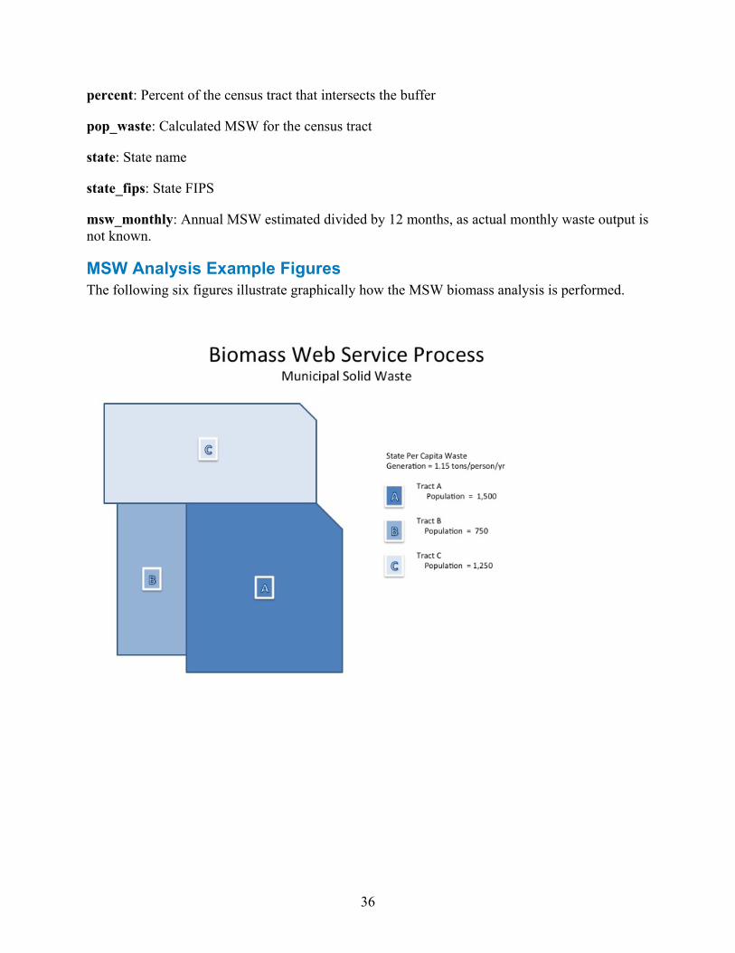
36

percent: Percent of the census tract that intersects the buffer

pop_waste: Calculated MSW for the census tract

state: State name

state_fips: State FIPS

msw_monthly: Annual MSW estimated divided by 12 months, as actual monthly waste output is not known.

MSW Analysis Example Figures The following six figures illustrate graphically how the MSW biomass analysis is performed.

37

38

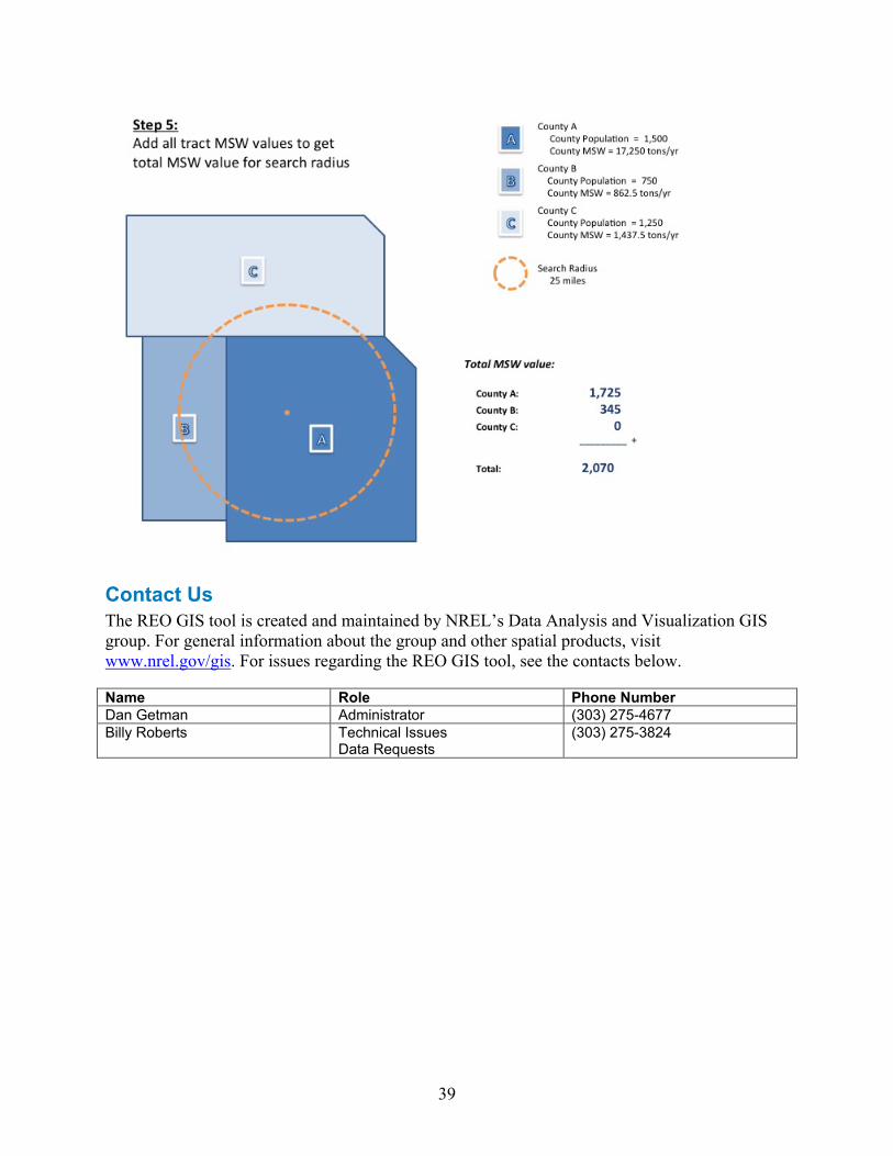
39

Contact Us The REO GIS tool is created and maintained by NREL’s Data Analysis and Visualization GIS group. For general information about the group and other spatial products, visit www.nrel.gov/gis. For issues regarding the REO GIS tool, see the contacts below.

Name Role Phone Number Dan Getman Administrator (303) 275-4677 Billy Roberts Technical Issues

Data Requests (303) 275-3824