WASHINGTON UNIVERSITY

THE HENRY EDWIN SEVER GRADUATE SCHOOL

DEPARTMENT OF CHEMICAL ENGINEERING

_________________________________

MASS AND ENERGY BALANCE FOR

A CORN-TO-ETHANOL PLANT

by

Fan Mei Prepared under the direction of Professors M. P. Dudukovic,

Martha Evans and Charles N. Carpenter

___________________________________

Thesis presented to the Henry Edwin Sever Graduate School of

Washington University in Partial fulfillment of the

requirements of the degree of

MASTER OF SCIENCE

May 2006

Saint Louis, Missouri

WASHINGTON UNIVERSITY THE HENRY EDWIN SEVER GRADUATE SCHOOL

DEPARTMENT OF CHEMICAL ENGINEERING

____________________________________

ABSTRACT

_____________________________________

MASS AND ENERGY BALANCE FOR

A CORN-TO-ETHANOL PLANT

by

Fan Mei

ADVISORS: Professor Milorad P. Dudukovic Professor Martha Evans

Professor Charles N. Carpenter

______________________________________

May 2006

Saint Louis, Missouri

_______________________________________

In this thesis, mass and energy balances models of a corn-to-ethanol plant using the dry mill process are developed. The information is provided to set up a mass balance and estimate energy demand using Aspen Hysys simulations. An easy-to-use Excel-based mass balance template which allows a user to modify the plant model and automatically recalculate results is also provided. The work result a viable alternative to an USDA Aspen Plus model. Also investigated was detailed information for manufacturing cost estimation.

ii

Contents

Tables…………………………………………………………………….v

Figures………………………………………………………………….vii

Acknowledgments..…………………………………………………...viii

1. Introduction…………………………………………………………1

1.1 Background………………………………………..…………1

1.2 Motivation and Objectives..……….……………...………….3

2. Material Balance for a Corn-to-Ethanol Process..…...…...………6

2.1 Process Overview………..…….……...…………...………...6

2.2 Material Balance Calculation………………………….....…11

2.3 Using the Excel-based Mass Balance….………...…….……12

2.4 Aspen Hysys Simulations..………………………….….……19

2.4.1 Saturation………………….………………..….……19

2.4.2 Cooking/Liquefaction…………..……………..…….20

2.4.3 Distillation/Dehydration……………..………..…….21

2.4.4 Evaporation……………………………..……..…….21

2.5 Conclusions...…………....………………………….….…...22

3. Energy Balance for a Corn-to-Ethanol Process…...……...…..….26

3.1 Overview……………………….……………………...……26

3.2 Energy Balance Calculations...……….………………......…29

iii

3.3 Energy Balance Evaluation………..……..…….……...……31

3.3.1 Cooking/Liquefaction Energy Consumption…..……33

3.3.2 Distillation/Dehydration and Evaporation Energy

Consumption………..…...………………………….34

3.3.3 Water Input in the Mashing Section………………...35

3.4 Electricity Demand……….………..……………….….……38

3.5 Results and Discussion…...………..……………….….……40

3.6 Conclusions…………………………………………………41

4. Economic Analysis for a Corn-to-Ethanol Process…………...….45

4.1 Literature Review...…………….……………………...……45

4.2 Manufacturing Costs Estimation…….………………......….47

4.3 Conclusions…………………………………………………49

5. Conclusions…………………………………………...………...….50

5.1 Overall summary....…………….……………………...……50

5.2 Conclusions………………………….………………......….51

5.3 Future Work…………………………………………………51

Appendix A – Streams Properties Estimation………..……………...53

Appendix B – Scale-up Feasibility…………………………….……...64

Appendix C – Block Flow Diagram… ……………………….………67

Appendix D – Excel-based Material Balance Template Guide…..…69

iv

Symbols…………………………………………………………………72

References………………………………………………………………73

Vita………………...……………………………………………………77

v

Tables

Table 2-1 Corn-to-Ethanol Dry Mill Process Description……….……….7

Table 2-2 Total Material Balance of Each Block……………...………...13

Table 2-3 Feed Corn Composition in Simulation………...……………..15

Table 2-4 Mass Fractions in Streams…………………...…………...…..15

Table 2-5 Ethanol Mass Fractions in Equilibrium Streams……….....….15

Table 2-6 Approximate Ranges for User-specified Values………..….…16

Table 2-7 Material Conservation Equations for Each Component……...18

Table 2-8 Main Input/Output for 30 MMgpy Plant…………………..…23

Table 3-1 Energy Consumption in Ethanol Production from Corn……..28

Table 3-2 Temperature and Pressure Range of the Unit Operation….….30

Table 3-3 Equipment Power Estimation Basis…………………….……38

Table 3-4 Electricity Demand of the Corn-to-Ethanol Plant…….……...39

Table 3-5 Summary of Total Energy Consumption……………….….…41

Table 3-6 Utility Demand by Type……………………………….…..…41

Table 3-7 Ethanol Plant Energy Use by Subsystems……….…………..43

Table 4-1 Typical Operating Costs, 2004………………………….…...46

Table 4-2 Financial Assumptions and Sensitivity Analysis Inputs….….47

Table 4-3 Manufacturing Costs for the 30 MMgpy Ethanol Plant….….48

Table A-1 Stream Properties…………………………………………....52

Table A-2 Solid Heat Capacity Methods in Aspen Properties…………54

vi

Table A-3 Corn Starch Hydrolyzate Viscosity………………………57

Table A-4 Glucose Solution Viscosities at Different Temperatures…58

Table A-5 Comparing Glucose Solution Viscosities Data…………..58

Table B-1 Scale-up Values for the Corn-to-ethanol Plant…………...61

Table B-2 Energy Consumption in Plants…………………………...62

Table C-1 Block Flow Diagram…………………………………..…63

vii

Figures

Figure 2-1 Block Flow Diagram of the Dry Mill Process……..…………6

Figure 2-2 Assumption Worksheet in Excel……..…………..……….....14

Figure 2-3 Unit Operation for Two-phase Saturation in Aspen Hysys….19

Figure 2-4 Unit Operation for Three-phase Saturation in Aspen Hysys ..20

Figure 2-5 Unit Operation for Cooking/Liquefaction in Aspen Hysys.....21

Figure 2-6 Single Block Flow Diagram of a Corn-to-ethanol Plant.........23

Figure 3-1 Energy Flow through an Ethanol Plant…………….………..27

Figure 3-2 Estimation Program for DDGS Dryer’s Mass and Energy

Balances……………………………………….………………………...31

Figure 3-3 Cooking/Liquefaction Simulation in Aspen Hysys……….....33

Figure 3-4 Evaporation Simulation in Aspen Hysys………………….....34

Figure 3-5 Distillation/Dehydration Simulation in Aspen Hysys…….....34

Figure 3-6 Water Inputs of the Mashing unit in the Dry Mill Plant….....35

Figure 3-7 Water Recycling Strategy of the 30 MMgpy Plant………….37

Figure 3-8 Energy Flow through the Corn-to-Ethanol Plant…………....44

Figure A-1 First steps for Selecting Physical Property Methods…...…..51

Figure A-2 Procedure for Polar and Nonelectrolyte components……….51

Figure A-3 Physical Properties Estimation Example…………………...60

viii

Acknowledgments

The author wishes to express her appreciation and gratitude to Professor Milorad

P. Dudukovic, Professor Martha Evans, and Professor Charles N. Carpenter for giving

the opportunity to participate in this research work. Their guidance and assistance are

deeply appreciated. The examining committee member Prof. P. A. Ramachandran is

recognized for his effort in reviewing and evaluating this research.

The National Corn-to-Ethanol Research Center in SIUE (South Illinois

University Edwardsville) is recognized for its assistance and support. The cooperation

of engineers and managers of SIUE was invaluable in this research.

Finally, the author would like to acknowledge the support and encouragement of

friends and family during her graduate study.

Fan Mei

Washington University in St. Louis

May 2006

1

Chapter 1

Introduction

1.1 Background

Alcoholic beverages are as old as human civilization. Thousand years ago, people

had known that grape juice could be converted to a nice beverage using a fermentation

method. It was only in the 19th century that the distiller manufacturing trade became an

industry with enormous production figures, due to improvements in the distillation

process. At the beginning of the 20th century, alcohol was used as fuel for various

combustion engines, especially in automobiles. Environmental problems resulted from

the prolonged and increased use of fossil feed stocks as an energy source. The eventual

exhaustion of the supply of crude oil is another problem associated with using fossil

fuels. Production of chemicals for fermentation and energy production from renewable

resources are considered as an alternative to petrochemical processes in recent years.

An alternative to petroleum is ethyl alcohol or ethanol. [20]

A successful example of large-scale alcohol technology is the Brazil ethanol

program, which was launched in the 1970s, and diminished the country’s dependence

on oil imports. The program is to provide 100% ethanol fuel using sugar cane. Brazil

leads the world in bioethanol production and consumption across the globe. All

2

automotive fuels sold in Brazil contain ethanol. More than 3.5 million cars run on 100%

ethanol fuel in Brazil. [35]

Ethanol is produced in the U.S. primarily from corn through a fermentation and

distillation process because corn is a mature farm product and its market price is stable.

In 2004, 11% of U. S. corn production was converted to ethanol. The ethanol

conversion rate from corn is typically in a range of 2.5 to 2.85 gallons of ethanol

produced from a bushel of corn (a bushel is equal to 56 lbs of corn). [43, 21] The ethanol

conversion rate depends on the starch content in corn, the saccharification and

fermentation conversions. To increase credit of the ethanol industry, the production

process also produces a high-value livestock feed (a concentrated mixture of protein,

fiber, vitamins and minerals) known as distillers dried grains with solubles (DDGS) and

carbon dioxide [35] DDGS contained a high value of protein and can be fed to cattle, pig

and chicken.

Two major processes used to produce bioethanol from corn are wet milling and

dry milling. In a wet mill process, grain is steeped and separated into starch, germ and

fiber components. In a dry mill process, grain is first grand into flour, and processed

without separation of starch. The dry milling process is becoming more common

because of a lower capital required to build a plant and easy operation. Dry milling is

the process modeled in this study.

In 2001, USDA (United States Department of Agriculture) developed an Aspen

Plus model for 30 MMgpy ethanol plant. Aspen Plus model is an overall model and

3

provides a good start for this study.

The U. S. ethanol industry had a 2004 annual production capacity of over 3

billion gallons. 59 companies are currently operating 76 active ethanol plants in the

U.S. [15] The majority of those companies are farmer owned cooperatives or limited

liability corporation dry-grind plants. Investments in farmer-owned ethanol

cooperatives generate new income. Farmers could receive an extra $6.6 billion of net

cash income over the next 15 years. [15]

The importance of an energy balance first surfaced in the mid-1970s when

ethanol began to receive attention as a gasoline extender. Mid-1970s studies analyzed

the energy benefits of substituting ethanol for gasoline and concluded that the net

energy value (NEV) of corn-to-ethanol was slightly negative. [10] In the late 1980s,

environmental concerns placed ethanol in the spotlight once again and energy balance

studies resurfaced. The USDA survey showed that the production process has

improved energy efficiency (energy required to produce ethanol/ energy released from

ethanol burned) resulting in a 10-30% net energy gain in 2002. [36]There is a

considerable amount of variation in the findings of these reports. These differences are

caused by different assumptions about farm production practices and corn conversion

to ethanol. Furthermore, the researchers used data from different time periods. Studies

using older data tend to overestimate energy use. Both ethanol manufacturing and farm

production technologies have become significantly more energy efficient in recent

4

times. It is often difficult to determine why results differ from study-to-study because

the reports often do not have critical details on calculation procedures.

The USDA survey shows that the average variable costs for dry mill plants were

$0.51 per gallon of ethanol produced for small plant size, $ 0.45 per gallon of ethanol

produced for medium plant size, and $ 0.36 per gallon of ethanol produced for large

plant size. [37]

1.2 Motivation and Objectives

Although the ethanol production industry is an old industry, it still has

opportunities for better design optimization. Computer-based process simulations

provide information for plant design, but most of process models for corn-to-ethanol

are proprietary or need improvement. The public information for corn-to-ethanol plant

modeling is too general. In addition to providing a useful tool for optimizing the

corn-to-ethanol process design, the experience gained from simulations can be

extended to improve existing production processes.

The objective in this study was to build a detailed mass and energy balance model

for the corn-to-ethanol dry mill process using public domain information. The model

should provide an easy-to-use, yet rigorous, tool for evaluation of mass and energy

balances in the corn-to-ethanol dry mill process. It also allows users to examine the

effects of changed process parameters on different operations and tests possible process

limitations. Results can be used as information for economic evaluations. This project

5

develops a methodology to estimate an energy balance from an Aspen Hysys computer

simulation and provides a more consistent estimate for the ethanol produced from corn.

6

Chapter 2

Material Balance for a Corn-to-Ethanol Process

2.1 Process Overview

The dry milling process can be divided into basic steps as presented in Figure 2-1.

The general process unit operations are described in Table 2-1 and Figure 1 in

Appendix C.

Figure 2-1: Block Flow Diagram of the Dry Mill Process

7

Table 2-1 Corn-to-Ethanol Dry Mill Process Description

Unit name Symbol Description

Milling A Corn passes through hammer mills that grind it into a fine powder called meal.

Mashing B

In this pre-cook section, water is mixed with the meal to form a mash. Water for mashing comes from the moisture in the corn, makeup water, recycled water (such as thin stillage), CO2 scrubber water, hot process condensate from the evaporators and flash tank condensate. [20] Added α-amylase in the slurry mixer begins the breakdown of starch to limit the maximum viscosity during cooking.

Cooking C

The treated slurry is cooked using one of two methods. In the first method, a hydroheater is used. Steam enters the system across a steam jet to heat the slurry. A 20-40 psi pressure drop as the steam enters the system helps to mechanically shear the starch molecules. The slurry is heated to 90-120 °C (194-248 °F) and held at that temperature for 8-10 minutes in a cook tube at the saturation pressure of 15-16 psig. The alternative method cooks the slurry at 125-140 °C (257-284 °F) using 150 psig steam in a cooking tube. In this case retention time is 6-8 minutes, under 40-50 psig pressure. No hydroheater is used. For both methods, high temperatures reduce bacteria levels in the mash.[14, 17, 24]

Liquefaction D

Liquefaction is the stage between the cooking and saccharification process. Gelatinized starch is partially hydrolyzed by α-amylase (or occasionally by an acid) to give soluble dextrin. The α-amylase converts all starch in the mash so it becomes a free-flowing liquid with reduced viscosity. A second injection of α-amylase is made because previously added α-amylase is denatured and or deactivated under cooking condition. The temperature is reduced to enable liquefaction at 86.7 °C (190 °F) and the pH value is maintained at 5.0 to 6.5. The liquid is cooled following the liquefaction phase with recovered heat used elsewhere in the process. [12, 20]

Yeast and yeast food are combined with liquefied mash in the yeast tank. The yeast tank is aerated so the

8

SSF (Simultaneous

Saccharification and

Fermentation)

F

yeast will propagate in the aerobic mode. While the yeast propagates, the SSF reactors are filled with cooled mash. Gluco-amylase is added to the mash to begin the process of saccharification, that is, the breakdown of dextrin to fermentable sugars. When the propagated yeast is ready, it is added to the fermentor and saccharification continues during fermentation. In the fermentation reaction, yeast ferments glucose to ethanol and carbon dioxide. [6, 40]

A typical corn-to-ethanol facility has three or more fermenters operating batchwise in staggered cycles of 48-72 hours until the mash is fully fermented. The fermentor operates anaerobically. Commercial yeast strains for ethanol production can effect fermentation at 32-35 °C (90-95 °F). At higher temperatures metabolic activity rapidly declines. Yeast prefers an acid pH and the optimum pH is 5.0-5.2. Released CO2 is removed from the system through the scrubber. [20,

24, 12, 43] The French chemist Joseph-Louis Gay Lussac established the mole stoichiometric equation in 1815[22] as C6H12O6->2CO2+2C2H5OH. Due to a variety of factors, this yield (51.11 parts ethanol (by weight)/100 parts glucose (by weight)) is not achieved in practice. This project uses the pratical yield from the USDA Aspen Plus model (the stoichiometric equations will be mentioned later). [22, 41]

Distillation /Dehydration H

Fermented mash, called "beer," contains 10-16 % alcohol by volume, [20, 35] as well as the non-fermentable solids from the corn and yeast cells. Mash is pumped into the continuous distillation (typically two columns) system where the alcohol is separated from the solids and most of the water as an azeotrope. Alcohol leaves the top of the first column as 60-80% ethanol (by volume). Water can be recycled to the α-amylase mixer from a stripper in the distillation column. [20]

The azeotropic 95.6% ethanol from the top of the second column passes through a system where the remaining water is removed.[43] The energy balance for this project assumes a molecular sieve is used to remove water in the ethanol to achieve 99.65% (weight) purity of ethanol. The ethanol product at this

9 stage is called anhydrous (pure, without water) ethanol. [20, 35, 43]

Denaturing involves adding a small amount (2-5% by weight) of a product, like gasoline, to the ethanol to meet state tax regulations.

Solids Separation J

The solids-containing bottoms from the beer column are called whole stillage (or thick stillage). Whole stillage total solids content is 7-14% (typically 8% dry solids) [43]. The whole stillage is separated by centrifuge into a somewhat diluted liquid (called thin stillage or backset, containing 1% or more suspended solids and 3% or more total solids) that will be partly recycled to the slurry mixer or fermenters. The balance of the thin stillage is concentrated to make syrup in the evaporation section. The centrifuged solids are typically called wet cake that contains approximately 65-75% moisture and 25-35% solids. Syrup from the evaporators is added to the wet cake to make DDGS (distillers dried grains with solubles) in the DDGS dryer. Wet cake, mixed with syrup is fed to the dryer, where it is dried to a final moisture content of 9-10%. [32] The moisture content in the feed to the dryer is decreased by recycling some dry product and mixing it with the wet cake and the syrup. This dryer feed “conditioning” prevents rapid fouling in the dryer, which may result in dryer fires. The best DDGS dryer performance occurs when the total feed moisture content is in the 25-30% range. [20] Corn normally contains 9-10% crude protein, but it is concentrated in DDGS to 28-30% (or more) crude protein. The DDGS concentrates nutrients (fat, protein and minerals) from corn by approximately a factor of 3. This makes DDGS a high-value animal feed. [20, 35, 26]

Evaporation E

Thin stillage is concentrated by evaporation to produce corn syrup. Syrup ranges from 25% to 50% total solids, and the model assumes 30% total solids as a typical operating target. Hot condensed water removed in evaporation (hot process condensate) can be reused in the mashing and fermentation sections. Corn syrup is added to the DDGS before drying to increase the caloric value. [20, 43]

In this study, we use a triple-effect evaporator as a

10 balance between capital costs and energy operating costs.

CO2 Scrubber K

VOC (volatile organic compounds), mainly ethanol, are removed from the CO2 produced during fermentation by a scrubber. Water passes through the scrubber in once-through operation. It is added to the mashing section of the process for ethanol recovery and water integration. CO2 can be compressed for sale to the carbonated beverage industry, or more commonly, is vented. [20, 35]

2.2 Material Balance Calculation

Material balances are a basis for process design. They determine quantities of raw

materials required and products produced. [39] For the complete process, balances of

individual process units determine process stream flows and compositions.

First, to resolve the material balance for the corn-to-ethanol plant, the unit

operations of the BFD (block flow diagram) must be defined. Boundaries of the BFD

define the input and output of the entire process. Boundaries of the individual blocks

define the connecting streams.

Second, the degree of detail for flow information is defined. For the

corn-to-ethanol process, some compositions of streams must be represented as

pseudo-components. The Aspen Plus corn-to-ethanol process simulation model from

USDA (United States Department of Agriculture) provides a convenient option. The

simulation model defines stream compositions in terms of 10 main ingredients. These

ingredients are water, glucose, CO2, ethanol, starch, C5poly, C6poly, protein, oil and

11

NFDS (non-fermentable dissoluble solids). The C5poly and C6poly ingredients

represent in general the carbohydrates (unfermentable sugars) with 5-carbon or

6-carbon monomers. [41]

Third, conservation equations are derived and assumptions chosen, to satisfy the

degrees of freedom, allowing the mass balance model to be run.

The USDA Aspen Plus model, [41] derived by Frank Taylor, is based on batch

fermentation, producing ethanol, dehydrated by molecular sieves, and DDGS dried in a

DDGS dryer. There are many advantages of an Aspen Plus model. The mash

concentration is adjustable as the process input. The annual ethanol production is

adjustable using a FORTRAN block scale factor. Also, the model provides a tool to

study the energy balance. However, the USDA model is incomplete in simulating water

reuse strategy and energy recovery. Running the model requires the Aspen Plus

environment and proficiency in Aspen Plus simulation. The ExcelTM mass balance

procedure described here provides an alternative useful tool for a chemical engineer to

analyze and manage the corn-to-ethanol plant.

2.3 Using the Excel-based Mass Balance

The following step-by-step procedure is a guide for use of the ExcelTM-based

mass balance.

Step 1. The block flow diagram of the corn to ethanol process is shown in Figure

2-1 and Figure 1 in Appendix C.

12

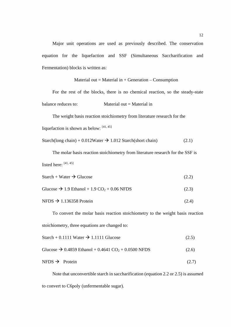
Major unit operations are used as previously described. The conservation

equation for the liquefaction and SSF (Simultaneous Saccharification and

Fermentation) blocks is written as:

Material out = Material in + Generation – Consumption

For the rest of the blocks, there is no chemical reaction, so the steady-state

balance reduces to: Material out = Material in

The weight basis reaction stoichiometry from literature research for the

liquefaction is shown as below: [41, 45]

Starch(long chain) + 0.012Water 1.012 Starch(short chain) (2.1)

The molar basis reaction stoichiometry from literature research for the SSF is

listed here: [41, 45]

Starch + Water Glucose (2.2)

Glucose 1.9 Ethanol + 1.9 CO2 + 0.06 NFDS (2.3)

NFDS 1.136358 Protein (2.4)

To convert the molar basis reaction stoichiometry to the weight basis reaction

stoichiometry, three equations are changed to:

Starch + 0.1111 Water 1.1111 Glucose (2.5)

Glucose 0.4859 Ethanol + 0.4641 CO2 + 0.0500 NFDS (2.6)

NFDS Protein (2.7)

Note that unconvertible starch in saccharification (equation 2.2 or 2.5) is assumed

to convert to C6poly (unfermentable sugar).

13

The yield is a function of starch composition in corn, saccharification and

fermentation conversions. The maximum yield is calculated, if starch conversion is

100% and glucose conversion is 100%. The typical maximum yield is 2.5 to 2.85

gallons ethanol per bushel corn due to different corn starch content. [20]

Table 2-2 Total Material Balance of Each Block

Block name Material balance equation

Milling oi AA =

Mashing oj

ji BB =∑=

7

1,

Cooking oj

ji CC =∑=

2

1,

Liquefaction ∑∑==

=3

1,

2

1,

kko

jji DD

SSF ∑∑==

=2

1,

3

1,

kko

jji FF

Distillation /Dehydration ∑∑

==

=4

1,

2

1,

kko

jji HH

Solids Separation ∑∑==

=3

1,

2

1,

kko

jji JJ

Evaporation ∑∑==

=2

1,

1

1,

kko

jji EE

CO2 Scrubber ∑∑==

=2

1,

3

1,

kko

jji KK

In this study, starch content is 59.5% (w). The maximum yield is 2.75 gallons

ethanol per bushel corn. Our practical yield is 2.7 gallons ethanol per bushel corn

because the maximum yield is not realistic in an ethanol plant. In Figure 2-1, the

14

subscript i/o signifies the material in or out. A material balance equation was written for

the total flow into and out of each process block, as shown in Table 2-2.

Step 2. Specify the process data. In the Excel-based mass balance model, the total

number of variables is 112, and the number of independent material balance equations

is 68. Hence, the number of variable to be specified for a unique solution (the degree of

freedom) is 44.

The example shown in Figure 2-2 is a list of assumption made for a 30 MMgpy

(million gallons per year). This number, 30 MMgpy is also the first specified variable

with an assumed conversion of 2.7 gallons of ethanol per bushel of corn.

Figure 2-2 Assumption Worksheet in Excel

There are 28 variables to be specified by the Aspen Plus model assumptions,

Aspen Hysys simulations results and the ethanol production rate. Variables include the

15

composition of corn shown in Table 2-3 (9 variables), the stoichiometry of the

liquefaction and SSF (8 variables), the mole fraction in streams shown in Table 2-4 (7

variables), the ethanol mass fraction in equilibrium streams shown in Table 2-5 (3

variables), and the percentage of flash steam from liquefaction tank (1 variable). The

Aspen Hysys simulation provides credible values for those variables chosen, and also

evaluates the sufficiency of those values, which will be discussed later in this chapter.

Note that the specified ethanol mass fractions in Bi2 (centrifuge/distillation water),

Do1 (liquefaction flash steam), and Ho1 (whole stillage) have no significant effect on

the overall mass balance calculation.

Table 2-3 Feed Corn Composition in Simulation [1]

ComponentNumber Component Content Molecular

weight Phase state in

Aspen 1 Water 15.0% 18.015 Liquid phase 2 Ethanol 0.0% 46.069 Liquid phase 3 CO2 0.0% 44.01 Liquid phase 4 Glucose 0.0% 180.156 Liquid phase 5 NFDS 6.8% 132.115 Liquid phase 6 Starch 59.5% 162.141 Solid phase 7 C5poly 5.1% 132.115 Solid phase 8 C6poly 2.6% 162.141 Solid phase 9 Protein 7.7% 132.115 Solid phase 10 Oil 3.4% 132.115 Solid phase

Total Corn 100% 72.314 Mixture

16 Table 2-4 Mass Fractions in Streams

Streams Symbol

Fo2 Ho2 Ko1 Hi2 Do1

Water 0.018 0.021 0.02 0.0506 0.9699 CO2 0.955 0.894 0.98 0 0

Ethanol 0.027 0.085 0 0.9494 0.0301

Table 2-5 Ethanol Mass Fractions in Equilibrium Streams

Streams Symbol Bi2 Ho1 Undenatured

ethanol

Ethanol mass fraction 0.0002 0.0002 0.9965

The remaining 15 specified variables are in typical literature ranges and shown in

Table 2-6. Note that the cooker steam rate is calculated using the heat balance sheet

derived by Prof. Heider [32], and evaluated by Aspen Hysys simulations. Details are

discussed later in this chapter. The units of the fresh water rate are converted from GPM

(gallons per minute) literature value to pph (pounds per hour).

Table 2-6 Approximate Ranges for User-specified Values [20, 43, 41, 18 and 32]

Assumption Range Value Cooker steam rate, pph[32] 5,000-40,000 22,000 Fresh water rate in CO2 scrubber, pph[20] 5,000-15,000 15,000 Percentage flash steam from liquefaction* 9.8-15% 11% Thin stillage ratio (split to mashing)[43] 12-20% 15% CO2 composition (%)from SSF to CO2 scrubber[20] 98-99% 98.5% Condensate discharge fraction[20] 0-10% 10% Percentage of the recycle HPC (hot process condensate) to mashing[20] 90-100% 100%

Percentage of the recycle HPC to fermentation[20] 0-10% 0% NFDS second reaction ratio[41] 26.9% 26.9% Solids percentage in thin stillage[20] 1-10% 7% Ratio of Liquefaction flash purge to liquefaction flash steam[41] Variable 30%

Saccharification percentage[20] 98-100% 98.5% Percentage of the sterile thin stillage[41] 25-35% 33.3% Starch and non-starch in mashing[20] 29-33% 30% Percentage of solids in syrup[20] 9-10% 10% DDGS moisture[32] Less than 50% 35%

* obtained from Aspen Hysys simulation

17

When users change the Excel-based mass balance variables to set up their own new

mass balance, equilibrium mass fractions cannot be changed. That means the ethanol

production rate (such as 30 MMgpy for this study), the denatured ethanol mass fraction

(Ho4 in Table 2-5), and the corn composition (Table 2-3) can be varied according to the

user’s objectives. The literature based variables (Table 2-6) can be modified according

to the specific plant design and technology. Those adjustable variables have a green

background in the Excel template as shown in Figure 2-2.

The mass balance was adjusted by modifying the assumption sheet “new assum”. In

the Excel worksheet “modified consumption”, Excel will automatically calculate plant

stream flow rates and compositions once the relevant data are entered or modified.

Step 3. Once a mass balance has been established, the model was used to study the

effect of changes in assumptions on plant performance. Based on a USDA model, the

Alcohol Textbook [20] and model testing, permissible ranges for loops in the system are

presented in Table 2-4, which can also be adjusted on the ExcelTM assumption sheet.

For example, water reuse in fuel ethanol plants is a complex process. Makeup

water, CO2 scrubber water, evaporation water, backset water, moisture in corn feed,

distillation water and flash tank condensate are all included in the water reuse streams.

When the user modifies the ExcelTM assumption sheet using the ranges listed in Table

2-6, the ExcelTM model will calculate the resulting different water flow rates. Note that

the saccharification and fermentation modeling will not reflect the effect of trace

default impurities in recycled water on yeast and enzyme performance. This is beyond

18

the scope of the current simple model. Also in the mass balance, all of the CO2

produced is assumed to leave the fermentor to go to the CO2 scrubber.

In every block, the overall mass balance and component balance must be

consistent. In blocks where no separation or reaction takes place, the problem is simple,

as illustrated in Table 2-7. Reaction stoichiometry for liquefaction, saccharification and

fermentation has been mentioned in equations (2.1) to (2.4). Separation units,

distillation and evaporation, are simulated by Aspen Hysys and further discussion is

provided in chapter 3.

In Table 2-7, xn,m means the concentration of component “m” in the stream “n”. In

the ExcelTM template, some xn,m values, specified in the “new assumption” worksheet,

are based on typical ranges in the literature and the Aspen Hysys simulation. Once all

required information is fixed in the feed and output streams, there are linear sets of

equations for each process unit. The equations can calculate a overall balance.

Table 2-7 Material Conservation Equations for Each Component Unit name Material balance equation

Milling mnomni xAxA ,, ×=×

Mashing mnomnj

ji xBxB ,,

7

1, ×=×∑

=

Cooking mnoj

mnji xCxC ,

2

1,, ×=×∑

=

Solids Separation mnk

komnj

ji xJxJ ,

3

1,,

2

1, ×=× ∑∑

==

CO2 Scrubber mnk

koj

mnji xKxK ,

2

1,

3

1,, ×=× ∑∑

==

19

Note that Appendix D provides the Excel-based mass balance template user

guide, and show users how to ‘quick’ start.

2.4 Aspen Hysys simulation

2.4.1 Saturation

In the mass balance calculation, some quantities such as the flow rate of the

cooker steam, the composition of the vapor from the CO2 scrubber, and the composition

of the gas phase from fermentor are not available in the literature. Some quantities, in

fact, depend upon a specific design. Thus, some type of a process simulation is

desirable, and Aspen Hysys was chosen. The Aspen Hysys simulations results are

comparable with a USDA Aspen Plus model. For example, the mass fraction of water in

the CO2 stream was 0.02% (w.) in the Aspen Hysys model and the USDA Aspen Plus

model.

To evaluate the water content in the vapor phase of the CO2 scrubber, it is

assumed that the CO2 stream is saturated with water at 1 atm and 29.3 ºC. [41] Using the

sample macro and extension “SATURATION” (solution ID# 110073) [1], the unit

operation “Saturation” shown in Figure 2-3 simulates the saturation process with water.

The mass fraction of water in the CO2 stream is 2%. This Unit Operation also can be

used to evaluate other two-phase (vapor and hydrocarbon) stream saturation conditions.

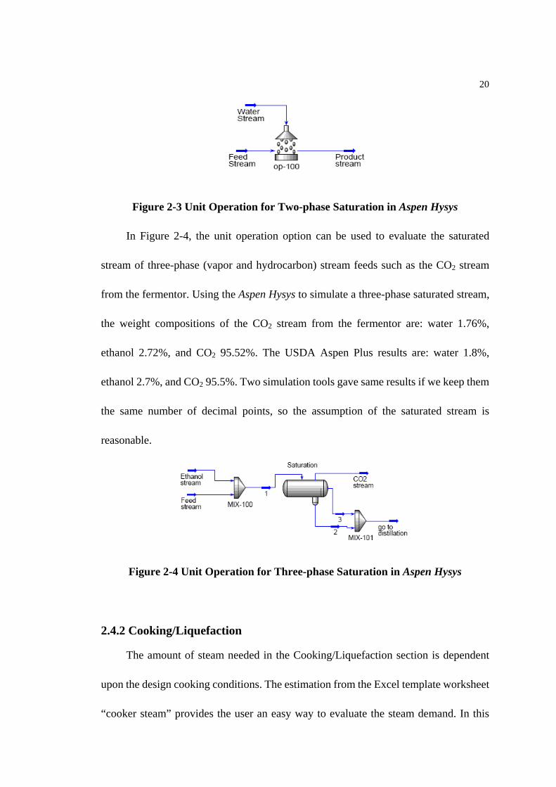
20

Figure 2-3 Unit Operation for Two-phase Saturation in Aspen Hysys

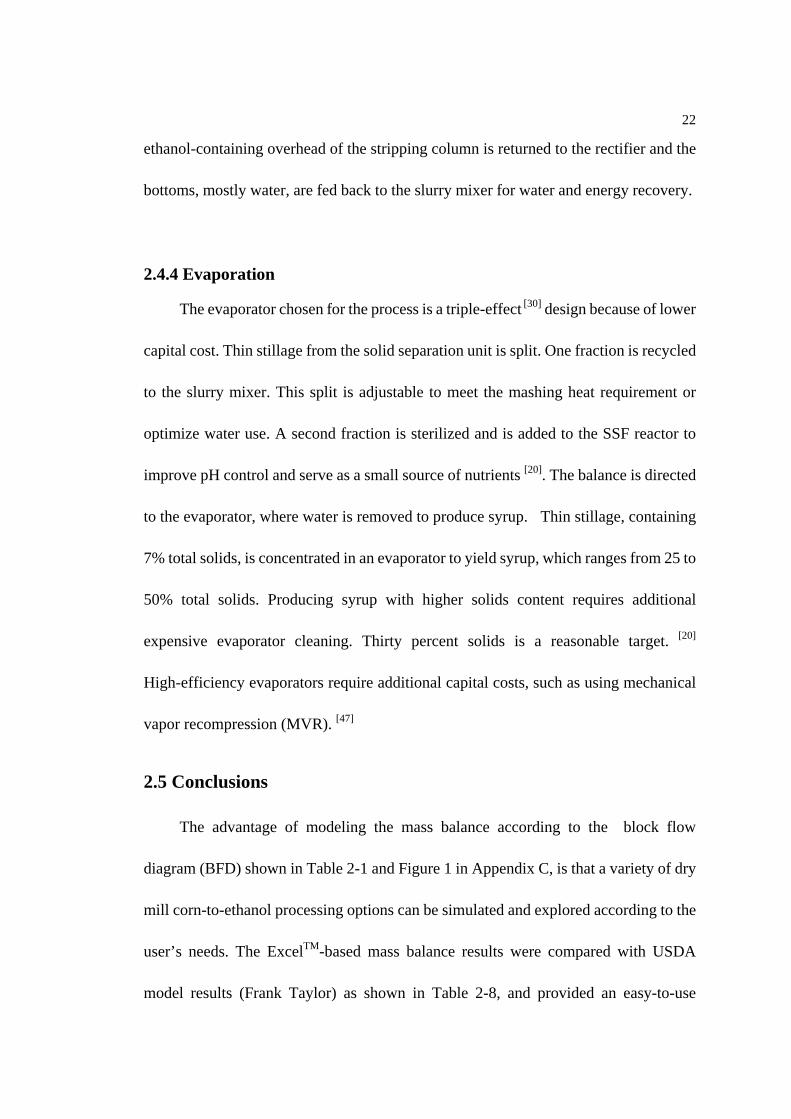
In Figure 2-4, the unit operation option can be used to evaluate the saturated

stream of three-phase (vapor and hydrocarbon) stream feeds such as the CO2 stream

from the fermentor. Using the Aspen Hysys to simulate a three-phase saturated stream,

the weight compositions of the CO2 stream from the fermentor are: water 1.76%,

ethanol 2.72%, and CO2 95.52%. The USDA Aspen Plus results are: water 1.8%,

ethanol 2.7%, and CO2 95.5%. Two simulation tools gave same results if we keep them

the same number of decimal points, so the assumption of the saturated stream is

reasonable.

Figure 2-4 Unit Operation for Three-phase Saturation in Aspen Hysys

2.4.2 Cooking/Liquefaction

The amount of steam needed in the Cooking/Liquefaction section is dependent

upon the design cooking conditions. The estimation from the Excel template worksheet

“cooker steam” provides the user an easy way to evaluate the steam demand. In this

21

study, the Cooking/Liquefaction operation is simulated using Aspen Hysys as shown in

Figure 2-5. Based on the 7 minutes holding tube design, flashing the cooked mash to

132.2 °C (270 °F), the cooker steam requirement is around 22,000 pph. Prof. Heider’s

estimate using steam tables was 21,754 pph. [32]

Figure 2-5 Unit Operation for Cooking/Liquefaction in Aspen Hysys

2.4.3 Distillation/Dehydration

The purpose of the distillation/dehydration unit is to purify ethanol to near 100%.

Preheated beer feed is degassed in a column, where CO2 is removed. The degassed

liquid is fed to the beer column. From the bottom of the beer column, whole stillage is

discharged to a solid separation unit after the beer/stillage heat exchanger. The

overhead stream from the beer column, containing about 43.6% (w) water and 53.4%

(w) ethanol, enters the rectifying column and is concentrated to 93.5% (w) ethanol. [43]

The bottoms from the rectifying column are pumped to the stripping column. The

22

ethanol-containing overhead of the stripping column is returned to the rectifier and the

bottoms, mostly water, are fed back to the slurry mixer for water and energy recovery.

2.4.4 Evaporation

The evaporator chosen for the process is a triple-effect [30] design because of lower

capital cost. Thin stillage from the solid separation unit is split. One fraction is recycled

to the slurry mixer. This split is adjustable to meet the mashing heat requirement or

optimize water use. A second fraction is sterilized and is added to the SSF reactor to

improve pH control and serve as a small source of nutrients [20]. The balance is directed

to the evaporator, where water is removed to produce syrup. Thin stillage, containing

7% total solids, is concentrated in an evaporator to yield syrup, which ranges from 25 to

50% total solids. Producing syrup with higher solids content requires additional

expensive evaporator cleaning. Thirty percent solids is a reasonable target. [20]

High-efficiency evaporators require additional capital costs, such as using mechanical

vapor recompression (MVR). [47]

2.5 Conclusions

The advantage of modeling the mass balance according to the block flow

diagram (BFD) shown in Table 2-1 and Figure 1 in Appendix C, is that a variety of dry

mill corn-to-ethanol processing options can be simulated and explored according to the

user’s needs. The ExcelTM-based mass balance results were compared with USDA

model results (Frank Taylor) as shown in Table 2-8, and provided an easy-to-use

23

program to evaluate the mass balance of any corn-to-ethanol plants. The USDA Aspen

Plus model can not be changed easily according to the user’s options due to the

complexity of the program.

Table 2-8 Main Input/Output for 30 MMgpy Plant

Input/Output USDA Aspen Plus, pph Our Research, pph Corn 74,659 76,376

Fresh water 30,000 34,500 Undenatured Ethanol 23,654 24,341

CO2 22,761 23,675 DDGS 24,640 28,427

To summarize the whole block flow diagram into a single block with inputs and

outputs, the simplified block is shown in Figure 2-6. This study goal is 30 MMgpy, so

the input of the block is corn and fresh water. Outputs are undenatured ethanol (99.5 %

(w)), CO2, and DDGS. Table 2-8 compared the input/output values for the whole 30

MMgpy plant. The USDA model used less corn than this study, because it is calculated

based on the maximum yield (2.75 gallons ethanol per bushel corn). The difference of

fresh water rate in USDA Aspen Plus model and our ExcelTM-based model is because

two models use different cooking section designs. The USDA model did not mention

any details of the cooking design and required 30,000 pph of water for cooking section.

In ExcelTM-based model, this study shows to use 22,000 pph of water in cooking

section and 12,500 pph of water in a CO2 scrubber. Note that in this study, zero

discharge is assumed. However, in the Excel-based mass balance program, we also

permitted a waste water (WW) discharge purge in case that the real operation condition

did not achieve zero discharge.

24

The ExcelTM-based model has an advantage in analyzing water reuse strategy

compared to the USDA model. The USDA model “recycles” nearly 100% of the water,

but it omits several intermediate streams. The USDA model assumes that the

evaporation section recycles a very large amount of water and produces syrup with

nearly 50% solids. On a practical level, the high percent solids would cause problems

with evaporator performance, such as maintenance down-time, lost production and

wasted energy.

Figure 2-6 Single Block Flow Diagram of a Corn-to-ethanol Plant

In the ExcelTM-based model, recycled water from the evaporation unit is nearly

44% of the mashing water quantity, because “hot process condensate” (HPC) from the

evaporation unit can recovery water and energy to mashing section. In total, the

distillation unit contributes nearly 30% water of the total water requirement for the

mashing unit. Details of the energy balance for evaporation, and

distillation/dehydration are discussed in Chapter 3.

The Excel-based model can be used to balance the energy consumption in the

mashing unit by adjusting recycle streams. However, the ExcelTM-based model requires

25

stream properties obtained from Aspen Properties. In this study, we examine the energy

consumption in the mashing unit using the method discussed in Appendix A.

The energy balance model, discussed in the following chapter, demonstrates

advantages of an Excel-based model.

A disadvantage of the Excel-based model is that the number of components is

fixed in this study. To change the components will change the mass balance equations.

The template can only handle stream compositions in terms of water, glucose, CO2,

ethanol, starch, C5poly, C6poly, protein, oil and NFDS (non-fermentable dissoluble

solids). In most cases, this composition assumption is sufficient for a corn-to-ethanol

process simulation. To study the lignocellulose-to-ethanol process, we need re-specify

additional stream components.

A similar mass balance could be derived with more components, but we judged

the components adequate for stoichiometry. More detail would not allow any current

advantage, but if DDGS research further characterizes DDGS composition for value

calculations, the model could be enhanced to predict DDGS quality and the economic

impact of feed corn composition on DDGS value.

The Excel-based mass balance model can provide valuable deductive

information. The mass balance is reported in a manner that is understandable,

supportable, flexible, and maintainable.

26

Chapter 3

Energy Balance for a Corn-to-Ethanol Process

3.1 Overview

While energy needs for ethanol production have decreased during the past 30

years, the availability of economical and reliable energy sources is essential for stable

operation of the facility. An emphasis on energy conservation at the facility will reduce

the burden on natural resources and the surrounding community.

When choosing a plant location, proximity to a sufficient supply of energy, such

as natural gas, coal, electricity and petroleum must be considered. The flexibility to

utilize more than one source of energy may be advantageous. Generally, electricity is

used for grinding and running electric motors. Thermal energy as steam is used for

cooking, liquefaction, ethanol recovery and dehydration. Natural gas thermal energy is

used for drying and stillage processing.

A public information-based calculation of the typical energy used to convert corn

to ethanol is based on a U.S. industry survey conducted in Sep. 2001 by BBI

International. [36] The survey was conducted by telephone interviews with 17 dry-mill

ethanol plants. The total production capacity of the plants in the survey is over 1.3

27

billion gallons or about 65% of industry’s current capacity [36]. On average, dry-mill

ethanol plants used 1.09 kWh of electricity and over 46,000 Btu of thermal energy per

gallon of ethanol. When energy losses in production and transportation of electricity

and natural gas are considered, the average dry-mill ethanol plant required about

48,772 Btu of primary energy per gallon of ethanol produced. The average conversion

rate for dry mill process was 2.64 gallons of ethanol per bushel of corn. [36]

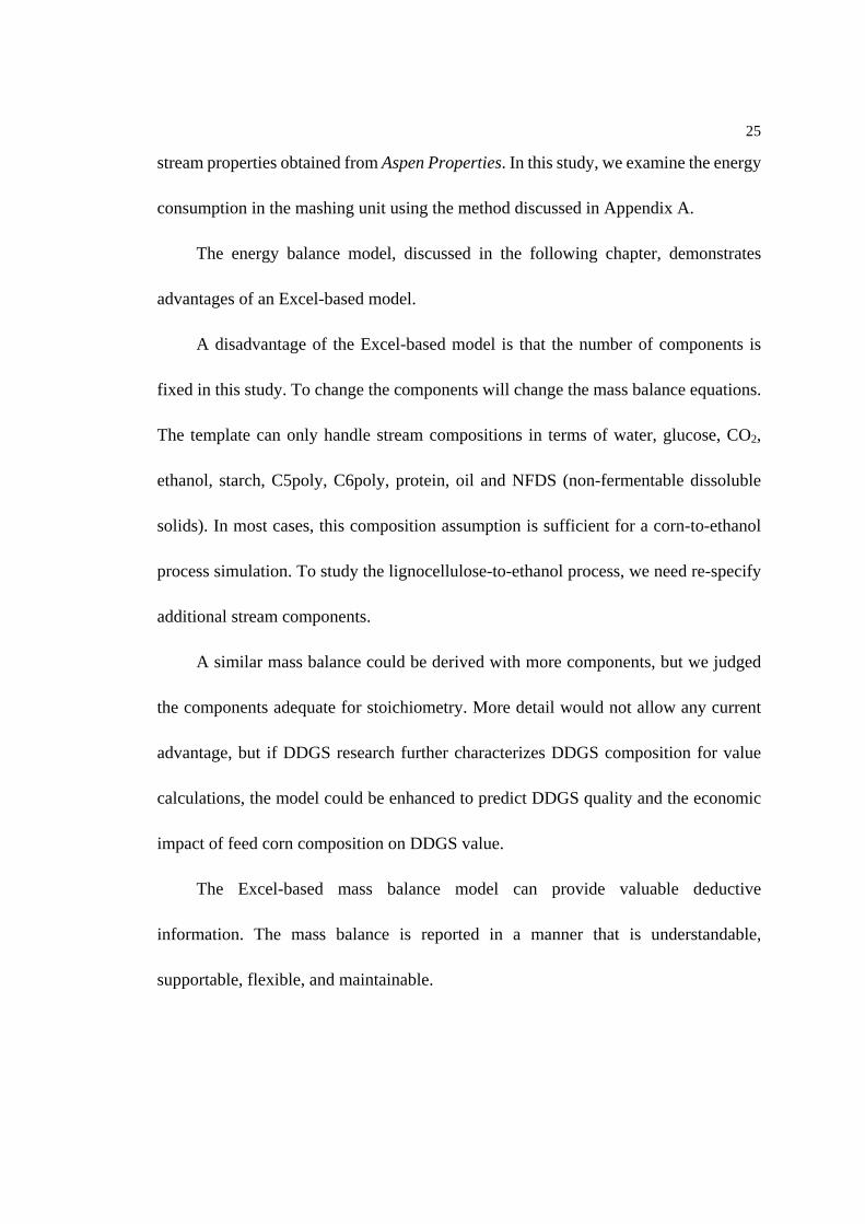
A typical energy usage in the ethanol plant is shown in Figure 3-1. [20] The

distillation/dehydration and evaporation units account for nearly 80% of the total

energy demand. [20]

Figure 3-1 Energy Flow through an Ethanol Plant

28

The energy demand in some classical processes for ethanol production from

corn is shown in Table 3-1. [35]

Table 3-1 Energy Demand in Ethanol Production from Corn, MJ/hlA[35]

Raw material Corn Ratio of stillage Recycling 30% 50%

Electrical energy 40 40

Thermal energy 170 150 Mashing Process

Sub total 210 190

Distillation* 700 700 Total 910 890

* 250 kg of steam per hlA (100 liters Alcohol) = 700 MJ per hlA for distillation of raw spirit (85% vol.). These data depend strongly on the distillation equipment used.

Reviewing Table 3-1, we conclude that the energy demand in ethanol production

is concentrated in the mashing process and distillation and that increasing the ratio of

stillage recycling decreases the total energy demand. This energy demand calculation

does not show the energy requirements of co-product (DDGS) production and also

does not provide any details for future modification. A more detailed energy

estimation method is required.

In this project, we model the major energy demand areas of the corn-to-ethanol

plant with an Aspen Hysys simulation, such as distillation/dehydration, evaporation,

and cooking sections. Aspen Hysys simulation results provide a reasonable source for

the mass balance assumption by incorporating the results of the mass balance from

Chapter 2 and estimate the energy demand for a plant design.

29

3.2 Energy Balance Calculations

In energy balance calculations, the energy considered includes the energy

content of the input and output streams, as well as the energy transferred as heat

from/to the surroundings and the work done by the system (negligible). In this study,

energy balances are made to determine energy requirements of the process which are

the heating, cooling and power required.

A general equation can be written for the open system at steady state:

Energy Input = Energy Output (3.1)

“Input” here signifies the total rate of transport of kinetic, potential and internal

energy by all process input streams plus the rates at which energy is transferred as heat

and work. “Output” is the total rate of energy transport by the output streams.

If Ej denotes the total rate of energy transport by the jth input or output stream of a

process, and Q and W are again defined as the rate of flow of heat and work into the

process, then equation (3.1) maybe written:

WQEEstreamsinput

j

streamsoutput

j +=− ∑∑ (3.2)

Let us use the symbol ∆ to denote total output minus total input, so that equation

(3.2) becomes:

WQEEH pk +=∆+∆+∆ (3.3)

H is the enthalpy of the stream, Ek is the kinetic energy and Ep is the potential

energy. The kinetic energy changes and potential energy changes are negligible

30

compared to those in the internal energy. For many processes, the work term will be

zero, or negligibly small, so that equation (3.3) simply becomes:

QH =∆ (3.4)

In this project, we choose to neglect the enthalpy of mixing and the effect of

pressure on ∆H (the enthalpy departure). As with the temperature and pressure ranges

for the units operations, we consider P0 = 1 atm, T0 = 25 ºC (77 ºF) as the standard

reference state, which is consistent with the Aspen Plus assumption.

For the blocks without reactions (cooking/liquefaction, distillation/dehydration,

and evaporation sections), we used Aspen Hysys model and estimate the energy

demand.

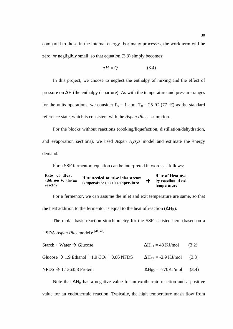
For a SSF fermentor, equation can be interpreted in words as follows:

For a fermentor, we can assume the inlet and exit temperature are same, so that

the heat addition to the fermentor is equal to the heat of reaction (∆HR).

The molar basis reaction stoichiometry for the SSF is listed here (based on a

USDA Aspen Plus model): [41, 45]

Starch + Water Glucose ∆HR1 = 43 KJ/mol (3.2)

Glucose 1.9 Ethanol + 1.9 CO2 + 0.06 NFDS ∆HR2 = -2.9 KJ/mol (3.3)

NFDS 1.136358 Protein ∆HR3 = -770KJ/mol (3.4)

Note that ∆HR has a negative value for an exothermic reaction and a positive

value for an endothermic reaction. Typically, the high temperature mash flow from

31

cooking/liquefaction section balances the energy requirement for the reaction of

starch converted to glucose. The lower temperature of the mash flowing to the SSF

reactor satisfies the required yeast conditions for a continuous fermentation. Therefore,

the energy demand in the SSF block consists of electrical energy supplied to meet

agitation and cooling water requirements.

3.3 Energy Balance Evaluation

First, for most streams, we need to specify operating temperatures and pressures

according to operating conditions. The general process temperature and pressure of

some unit operations are in Table 3-2. [20, 43]

Table 3-2 Temperature and Pressure Range of the Unit Operation [20, 43]

Block name Symbol Temperature, °C Pressure, atm

Milling A 20 1 Mashing B 40-60 2.7

SSF F 30-32 1 CO2 scrubber K 25 1

Solids Separation J 60-80 1

Distillation/dehydration, evaporation, and cooking/liquefaction sections are

simulated by Aspen Hysys and will be discussed later in this chapter. The DDGS dryer

produces DDGS and requires a significant amount of energy input. Typically, the

energy demand of the DDGS dryer depends on the overall DDGS package design and

the choice of vendor. In this project, we use the “Continuous Dryer Program” [32]

derived by Prof. Heider to calculate the energy cost of the DDGS dryer as shown in

Figure 3-2. The energy demand of the DDGS dryer is 50.1 MMBtu/hr for a 30 MMgpy

32

plant. This result is comparable to the simple estimate from the Ventilex Company

(1280 Btu / lb water evaporated as efficiency for 49.6 MMBtu/hr). [31]

Figure 3-2 Estimation Program for DDGS Dryer’s Mass and Energy Balances

Second, we need to evaluate the enthalpy contents of all of the streams to

determine heating and cooling duties for the heat exchangers of the mashing mixer. To

maintain consistency with the mass balance and reduce the need to re-work the entire

sections, the described enthalpy content estimation is based on the Microsoft ExcelTM

template.

Moreover, once heat duties are known, we are able to consider heat integration

among the process streams.

Finally, to explore the process design in greater detail, we can consider the power

requirements of all equipment in that we can get the electricity demand for the whole

plant. The results also can be used to size heat exchangers for plant design.

33

3.3.1 Cooking/Liquefaction Energy Demand[14]

Mash (around 60 ºC) from the slurry mixer is heated to 132.2 ºC (270 ºF) by 150

psig saturated steam in the cooking tube. The cooked mash is flashed to 15 psig to

produce saturated steam and a concentrated mash in the flash tank. Then the slurry is

cooled to 195 ºF for the liquefaction by flashing into a vacuum. After the liquefaction

tank, the vapor passes through a steam ejector. Steam at 150 psig is fed to the ejector

along with the uncondensed vapor, and the resulting mixture is sent to a condenser

operating at 15 psig. All condensates from these units are pumped back to the slurry

mixer for energy and water recovery and the negligible amount of gas (including air

and CO2, less than 0.001% (w.) of the slurry flow rate) is vented. The energy demand,

calculated from the 150 psig saturated steam demand converted to natural gas

demand, is 31.7 MMBtu/hr. (The boiler efficiency factor to convert natural gas Btu to

steam Btu is 0.82.)[20]

Figure 3-3 Cooking/Liquefaction Simulation in Aspen Hysys

34

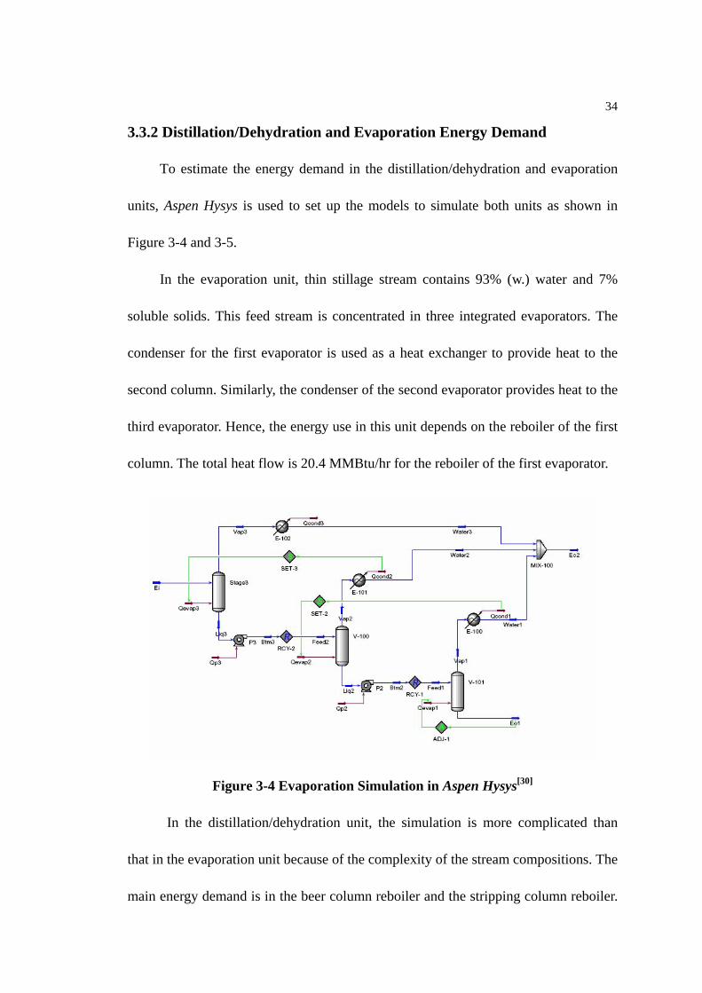
3.3.2 Distillation/Dehydration and Evaporation Energy Demand

To estimate the energy demand in the distillation/dehydration and evaporation

units, Aspen Hysys is used to set up the models to simulate both units as shown in

Figure 3-4 and 3-5.

In the evaporation unit, thin stillage stream contains 93% (w.) water and 7%

soluble solids. This feed stream is concentrated in three integrated evaporators. The

condenser for the first evaporator is used as a heat exchanger to provide heat to the

second column. Similarly, the condenser of the second evaporator provides heat to the

third evaporator. Hence, the energy use in this unit depends on the reboiler of the first

column. The total heat flow is 20.4 MMBtu/hr for the reboiler of the first evaporator.

Figure 3-4 Evaporation Simulation in Aspen Hysys[30]

In the distillation/dehydration unit, the simulation is more complicated than

that in the evaporation unit because of the complexity of the stream compositions. The

main energy demand is in the beer column reboiler and the stripping column reboiler.

35

The total heat demand is 53.5 MMBtu/hr for the reboilers.

Figure 3-5 Distillation/Dehydration Simulation in Aspen Hysys[30]

3.3.3 Water Input in the Mashing Section

The mashing unit of the dry milling fuel alcohol plant is schematically shown in

Figure 3-6. In this unit, water, from a variety of sources, is mixed with corn to form

mash. The temperature in the mashing unit is in the 40 to 60 ºC (104 to140 ºF) range,

which provides a suitable environment for the enzyme. The enzyme manufacturer will

specify optimal conditions for their product. [20]

In Figure 3-6, the total water entering the system includes the moisture in the corn

feed, well water (including the regular make-up water and the liquefaction flash steam)

and recycle water such as thin stillage, evaporator condensate and CO2 scrubber

water.[20]

36

MashingB

Evap

orat

or

cond

ensa

te

Thin

stil

lage

Water (Distillation)

Water (Grain Moisture)

CO

2sc

rubb

er

wat

er

Mak

eup

wat

erLi

quef

actio

n fla

sh s

team

Bi1

Bi5 Bi7 Bi6

Bi2

Bi3 Bi4

Figure 3-6 Water Inputs of the Mashing unit in the Dry Mill Plant

The mashing unit operating temperature is assumed to be 60 °C (or around 145

°F), a typical recommendation of the α-amylase manufacturer. [43] The hot process

streams such as thin stillage and evaporator condensate provide not only a portion of

the required liquid (nearly 45% of the total water), but also provide the energy needed

in the unit. The percentage of thin stillage that should be used for maximum efficiency

is typically in the range of 30 to 40% (solids content), but should generally not exceed

50%. Too high of a recycle component allows the accumulation of trace contaminants

in the process, which adversely affect performance of yeast and enzymes.

Water entering the mashing unit as corn moisture is relatively easy to quantify. A

typical moisture level of #2 yellow dent corn is 15% (weight). [33] After cooking, the

mash has 29-33% solids. For this study, we assume that the mash has 30% solids.

Increasing the cooker steam volume gelatinizes the starch in the slurry.

Overheating the slurry will waste energy in both the cooker steam production and

require additional cooling water. For the 30 MMgpy ethanol plant, the range of the

37

cooker steam is required from 5,000 to 40,000 pph. [20, 43] The wide range of cooker

steam requirements is determined by the energy demand which vary using different

Cooking/Liquefaction designs. Higher cooker temperature (284 ºF) and longer holding

time (10 minutes) decrease the required amount of cooking steam to nearly 5,000 pph,

but require more energy to keep the cooking tube at the higher temperature and also

need extra 17,000 pph make-up water to the mashing section.

A lower cooker temperature (220 ºF) operation increases the required amount of

cooking steam to nearly 33,000 pph, but it causes addition of extra water in the mashing

section. The lower temperature operation also dilutes the ethanol content in SSF, in

addition, increases the energy demand in the distillation and evaporation sections.

The mentioned minimum and maximum cooker steam values are estimated using

a ‘zero discharge’ assumption. That means an anaerobic biomethanator is required in

the plant.

When the plant includes a biomethanator, organic materials in recycling water

streams are not dispersed onto the field or into SSF where they have a BOD (biological

oxygen demand) or COD (chemical oxygen demand) impact on both the surrounding

environment and microbiological fermentation. [20] If biomethanator water is

discharged (assume 10% of evaporation condensate), make-up water volumes or

cooker steams value are increased nearly 6,000 pph as needed. Usually, adding more

cooker steams is preferred, because adding make-up water causes extra energy in

pumps and cooking/liquefaction section. So a maximum value of cooker steam is set as

38

40,000 pph for the 30 MMgpy plant.

In this project, we used the Cooking/Liquefaction design as described in Chapter

2, and the required steam rate is 22,000 pph. [14] The water recycling strategy is shown

as Figure 3-7. The natural gas energy demand in the mixing section is 2.4 MMBtu.

Water Percentage

Bi1-8.7%Bi2-15.6%

Bi3-9.5%Bi4-0.1%

Bi5-43.7%

Bi6-9.0%

Bi7-13.5%

Bi1-Grain moisture Bi2-Distillation (SC)

Bi3-Scrbr Water Bi4-Makeup water

Bi5-Evaporation Condensate Bi6-Liq flash steam

Bi7-Thin stillage Figure 3-7 Water Recycling Strategy of the 30 MMgpy Plant

3.4 Electricity Demand

Electricity in a modern mid-sized plant is expected to be between 0.7 and 1.2

kWh/ undenatured gallon ethanol. [20]

Table 3-3 Equipment Power Estimation Basis [32]

Items Horsepower (each) Blower 20

Vertical conveyor 15 Hammer mill 250

Molecular sieves motor 10 Centrifuge bowl motor 150 Centrifuge scroll motor 20

Agitator estimation 0.1 HP/1000 gal (SSF) 0.1 HP/1000 gal (Beer well) 0.3 HP/1000 gal (rest of vessels)

Fan 50 CIP pump 20

39

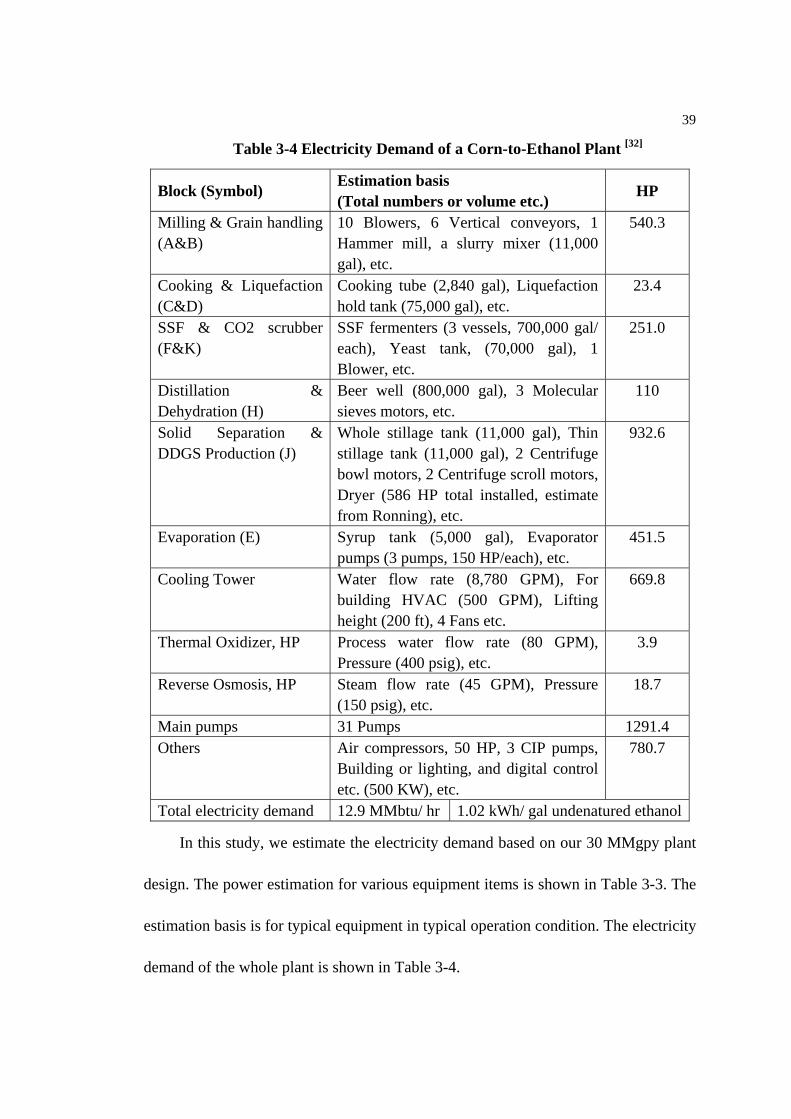
Table 3-4 Electricity Demand of a Corn-to-Ethanol Plant [32]

Block (Symbol) Estimation basis (Total numbers or volume etc.) HP

Milling & Grain handling (A&B)

10 Blowers, 6 Vertical conveyors, 1 Hammer mill, a slurry mixer (11,000 gal), etc.

540.3

Cooking & Liquefaction (C&D)

Cooking tube (2,840 gal), Liquefaction hold tank (75,000 gal), etc.

23.4

SSF & CO2 scrubber (F&K)

SSF fermenters (3 vessels, 700,000 gal/ each), Yeast tank, (70,000 gal), 1 Blower, etc.

251.0

Distillation & Dehydration (H)

Beer well (800,000 gal), 3 Molecular sieves motors, etc.

110

Solid Separation & DDGS Production (J)

Whole stillage tank (11,000 gal), Thin stillage tank (11,000 gal), 2 Centrifuge bowl motors, 2 Centrifuge scroll motors, Dryer (586 HP total installed, estimate from Ronning), etc.

932.6

Evaporation (E) Syrup tank (5,000 gal), Evaporator pumps (3 pumps, 150 HP/each), etc.

451.5

Cooling Tower Water flow rate (8,780 GPM), For building HVAC (500 GPM), Lifting height (200 ft), 4 Fans etc.

669.8

Thermal Oxidizer, HP Process water flow rate (80 GPM), Pressure (400 psig), etc.

3.9

Reverse Osmosis, HP Steam flow rate (45 GPM), Pressure (150 psig), etc.

18.7

Main pumps 31 Pumps 1291.4 Others Air compressors, 50 HP, 3 CIP pumps,

Building or lighting, and digital control etc. (500 KW), etc.

780.7

Total electricity demand 12.9 MMbtu/ hr 1.02 kWh/ gal undenatured ethanol

In this study, we estimate the electricity demand based on our 30 MMgpy plant

design. The power estimation for various equipment items is shown in Table 3-3. The

estimation basis is for typical equipment in typical operation condition. The electricity

demand of the whole plant is shown in Table 3-4.

40

3.5 Results and Discussion

A comparison of the energy demand calculated from different studies is shown in

Table 3-5. In this paper, we consider only the energy demand for ethanol manufacture.

The comparison did not include the energy demand in corn farming, storage and

fertilizer inputs. Differences among these studies are from various assumptions about

corn yields, ethanol conversion, and the data collection periods used. Our energy

estimation is based on published information of corn-to-ethanol plant designs. USDA’s

energy balance of the corn-to-ethanol process was based on published data in 1995,

2002, and 2003 in the American Society of Agricultural Engineers (ASAE). [38]

Pimentel’s analysis has a different basis. Some higher and some lower heating

values (HHV and LHV) were assumed. The energy estimate for ethanol conversion in

Pimentel’s 1991 and 2001 studies are over 30,000 Btu/gal of ethanol higher than the

Wang et al.[46] estimate, and over 20,000 Btu/gal of ethanol higher than this study. This

stems from Pimentel’s inclusion of energy expended on capital equipment and energy

for steel, cement, and other materials used to construct the ethanol plant, components

not included in most other studies. Pimentel also used a low ethanol conversion rate of

2.50 gallons of ethanol per bushel of corn.

Although John Meredith[20] mentioned that the modern fuel ethanol plant

approaches energy usage ratios of 36,000 Btu/gal and 0.7 kWh/gal[20] and those results

are close to Wang et al.[46]’s values in Table 3-5, the details of their energy balance

calculation were not mentioned. They assumed that newly built ethanol plants were

41

generally 30% more energy efficient than old plants and modified previous results to

the new energy demand rates by an efficiency parameter. [46]

Table 3-5 Summary of Total Energy Demand [10, 23, 29, 36]

Study/year Corn-to-Ethanol conversion rate,

gal/bu

Ethanol conversion process, Btu/gal

Pimentel (1991) 2.50 73,687 Pimentel (2001) 2.50 75,118

Keeney and Deluca (1992) 2.56 48,470 Marland and Turhollow

(1990) 2.50 50,105

Lorenz and Morris (1995) 2.55 53,956 Ho (1989) NR 57,000

Wang et. al. (1999) 2.55 40,850 Agri. And Agri-Food

Cannada (1999) 2.69 50,415

Shapouri et al. (1995) 2.53 53,277 Shapouri et al. (2002) 2.66 51,779

This study (2005) 2.70 46,114

3.6 Conclusions

The required utilities for this study are shown in Table 3-6.

Table 3-6 Utility Demand by Type

Utility Reacted water Electricity

Cooling water/chilled

water Natural gas

Quantity 34,500pph 1.02 kWh 20,000 Btu/gal ethanol

42,623 Btu//gal ethanol

Water used in the corn-to-ethanol plant includes two parts. One part is fresh

water. The first part of water demand (called reacted water) is in mashing section and

the CO2 scrubber. In the CO2 scrubber, fresh water absorbs ethanol and returns it to the

process for eventual recovery. Less than 4.0 % (w.) fresh water entering the CO2

42

scrubber is vented. The second part of water demand is for steam generation. Dry mills

use natural gas to provide energy demand for reboilers and 150 psig steam for cooking.

In this study, 22,000 pph of 150 psig cooking steam is injected into the process and is

counted as a part of the reacted water. Nearly 13.2 % of total reacted water will be

consumed in the SSF reactor. Note that the cooling or chilled water, which is used to

keep a suitable temperature for SSF reactors, and the heat duty for the heat exchanger

and condensers, is not included in the water demand calculation, because it is a minor

quantity compared to the overall process water demand.

The majority of the electricity is used for milling the corn, running motors,

cooling tower, and pumps, for distillation, dehydration and solid separation and

evaporation sections. According to the previous section, the 30 MMgpy corn-to-ethanol

plant will require 1.02 kWh / gal undenatured ethanol of electricity while operating.

The waste heat boiler for the thermal oxidizer or regenerative thermal oxidizer,

which is part of the dryer package, uses natural gas to oxidize the dryer offgas and

produce the steam needed by the corn to ethanol plant. Natural gas is also used to fuel

the dryer air heater.

Table 3-7 summarizes the energy flows through the major subsystems in the

process. Dryhouse operations include solid separation, evaporation and DDGS

processing. The primary thermal energy use points are distillation/dehydration and the

dry house followed by the cooking process.

43

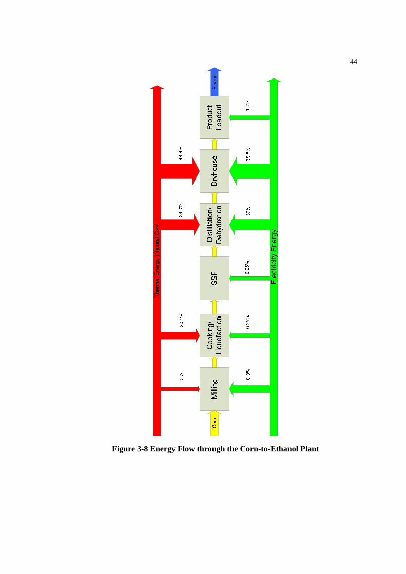
Table 3-7 Ethanol Plant Energy Use by Subsystems

Natural gas

MMBtu/hr percentage Electricity cost

percentage

Milling 2.4 1.5% 10% Cooking/Liquefaction 31.7 20.1% 6.25%

SSF Neg. 0% 6.25% Distillation/Dehydration 53.5 34.0% 37%

Dryhouse 70.0 44.4% 39.5% Product loadout 0 0% 1%

Total 157.5 100% 1.02 kWh

In this study, the energy flow through the corn-to-ethanol plant is shown in Figure

3-8. This result is comparable with the typical energy flow diagram shown in Figure

3-1. The distillation/dehydration and dryhouse units account for nearly 80% of the total

energy demand.

The estimated net energy value (NEV) of corn ethanol was 21,105 Btu/gal in

2002 USDA survey (Shapouri et al.).[36] 2002 USDA survey used higher heating values

(HHV) for measuring energy. Higher heating value, also called gross heating value, is

the standard heat of combustion referenced to water in combustion exhaust as liquid

water. Lower heating value (LHV), also called net heat of combustion, is the standard

heat of combustion referenced to water in combustion exhaust as water vapor. Keeney

and Deluca [48] used 74,680 Btu per gallon of ethanol as LHV, and Lorenz and

Morris[49] used 84,100 Btu per gallon of ethanol as HHV. Energy demand of the ethanol

conversion process in this study is about 5,000 Btu/gal lower than 2002 USDA survey

result. We can expect the net energy value in this study is higher than 2002 USDA

survey result.

44

Figure 3-8 Energy Flow through the Corn-to-Ethanol Plant

45

Chapter 4

Economic Analysis for a Corn-to-Ethanol Process

4.1 Literature Review

The total cost of producing ethanol has two main elements: capital cost and

manufacturing cost. [42] The capital cost of a corn-to-ethanol plant is determined partly

by the plant design, equipment chosen, and installation cost. Larger plants have a scale

advantage. Capital costs per gallon drop from $ 1.80 per gallon ethanol for a 15

MMgpy plant to $ 1.40 per gallon ethanol for a 50 MMgpy plant. [37] Manufacturing

costs are associated with the day-to-day operation of a corn-to-ethanol plant. Important

operating costs are from raw material (corn), natural gas, other utilities and other fixed

and variable costs. Using mass and energy balances, detailed information is provided

for the manufacturing costs in this study..

Ethanol plant manufacturing costs are often determined by tracking the cost per

gallon of ethanol (99.5% by weight) produced as a “Unit Cost”. [5] Table 4-1 shows

some typical unit operating costs for small (producing less than 30 MMgpy) and large

plants (producing up to 200 MMgpy). These unit operating costs do not include corn

costs ($2.25 per bushel of corn) or credit taken for the production of co-products. The

co-products are DDGS ($90 per ton of corn, and $0.27 per gallon of ethanol) and CO2

(be vented in this study). [25]

46

Table 4-1 Typical Operating Costs, US$ per Gallon of Ethanol Produced, 2004[5]

< 30 MMgpy Up to 200 MMgpy

Energy 0.198 0.178

Chemicals 0.134 0.088

Labor 0.090 0.060

Fixed and variable costs 0.106 0.085

Total operating costs 0.528 0.411

In Table 4-1, energy has the largest cost contribution ranging from $ 0.12 to $

0.22 per gallon of ethanol produced. [5] In the corn-to-ethanol dry mill process, energy

consumption includes electrical power and fuel, typically natural gas. The power and

fuel are consumed in the DDGS dryers and in the generation of steam which is used as

a heat source in the cooking/liquefaction, evaporation and distillation processes.

Chemical costs represent the second largest contributor to the total operating cost

and range from $ 0.06 to $ 0.14 per gallon of ethanol produced. [5] Chemical

consumption includes yeast, yeast nutrients, denaturant, α-amlyase for starch

liquefaction, gluco-amylase for the conversion of the starch to fermentable sugar.

Consumed also are a variety of antibiotics, disinfectants, water treating chemicals and

pH adjustment additives.

The cost of labor is a significant portion of the total operating costs and can range

from $ 0.04 to $ 0.11 per gallon of ethanol produced, depending on the facility type and

plant size. [5] Smaller facilities may have staffing levels of 0.3 people per MMgpy,

while at larger facilities the staffing may be as low as 0.1 people per MMgpy.

Other fixed and variable costs include repair and maintenance, water and sewage,

and fixed costs (depreciation, local taxes and insurance, and plant overhead costs) etc.

The cost of other fixed and variable costs range from $ 0.06- $0.12 per gallon of ethanol

produced. [37]

USDA contracted with Bryan and Bryan Inc. International to conduct a survey of

ethanol production costs during 1999 and early 2000. [37] Cash operating expenses

47

include electricity, fuels, waste management, water, enzymes, yeast, chemicals, repair

and maintenance, labor, management, administration, taxes, and insurance.

4.2 Manufacturing Costs Estimation

Location is the most important factor contributing to a business success. The

same holds true for an ethanol plant. An ethanol facility needs access to natural gas or

some other energy source. The facility also requires adequate electricity, water supply,

and other inputs.

The East Kansas Agri-Engery (EKAE) Steering Committee has contracted with

BBI International to complete a study to thoroughly assess the feasibility of

constructing a dry mill ethanol plant in Garnett, Kansas. [13] In this study, the economic

analysis used the price data for Garnett, Kansas.

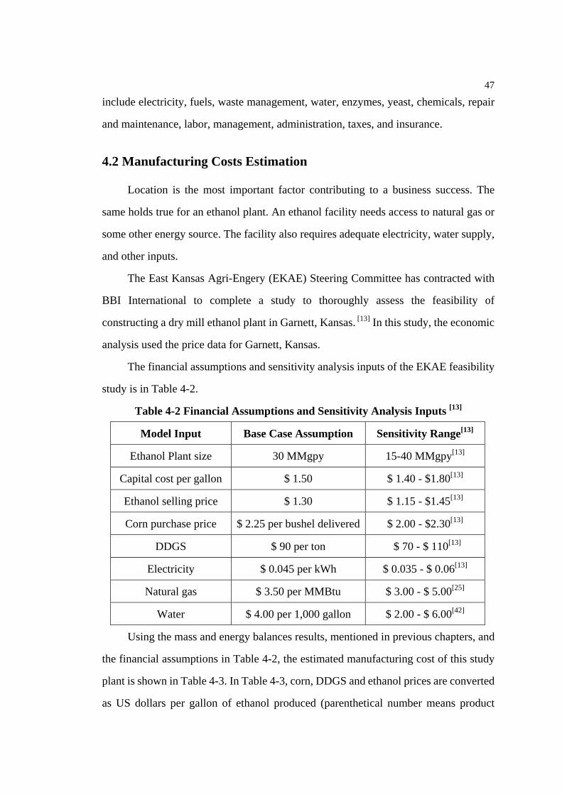
The financial assumptions and sensitivity analysis inputs of the EKAE feasibility

study is in Table 4-2.

Table 4-2 Financial Assumptions and Sensitivity Analysis Inputs [13]

Model Input Base Case Assumption Sensitivity Range[13]

Ethanol Plant size 30 MMgpy 15-40 MMgpy[13]

Capital cost per gallon $ 1.50 $ 1.40 - $1.80[13]

Ethanol selling price $ 1.30 $ 1.15 - $1.45[13]

Corn purchase price $ 2.25 per bushel delivered $ 2.00 - $2.30[13]

DDGS $ 90 per ton $ 70 - $ 110[13]

Electricity $ 0.045 per kWh $ 0.035 - $ 0.06[13]

Natural gas $ 3.50 per MMBtu $ 3.00 - $ 5.00[25]

Water $ 4.00 per 1,000 gallon $ 2.00 - $ 6.00[42]

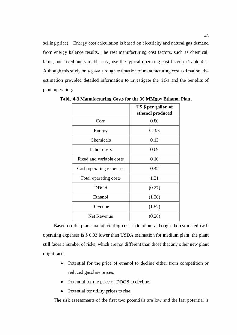
Using the mass and energy balances results, mentioned in previous chapters, and

the financial assumptions in Table 4-2, the estimated manufacturing cost of this study

plant is shown in Table 4-3. In Table 4-3, corn, DDGS and ethanol prices are converted

as US dollars per gallon of ethanol produced (parenthetical number means product

48

selling price). Energy cost calculation is based on electricity and natural gas demand

from energy balance results. The rest manufacturing cost factors, such as chemical,

labor, and fixed and variable cost, use the typical operating cost listed in Table 4-1.

Although this study only gave a rough estimation of manufacturing cost estimation, the

estimation provided detailed information to investigate the risks and the benefits of

plant operating.

Table 4-3 Manufacturing Costs for the 30 MMgpy Ethanol Plant

US $ per gallon of ethanol produced

Corn 0.80

Energy 0.195

Chemicals 0.13

Labor costs 0.09

Fixed and variable costs 0.10

Cash operating expenses 0.42

Total operating costs 1.21

DDGS (0.27)

Ethanol (1.30)

Revenue (1.57)

Net Revenue (0.26)

Based on the plant manufacturing cost estimation, although the estimated cash

operating expenses is $ 0.03 lower than USDA estimation for medium plant, the plant

still faces a number of risks, which are not different than those that any other new plant

might face.

• Potential for the price of ethanol to decline either from competition or

reduced gasoline prices.

• Potential for the price of DDGS to decline.

• Potential for utility prices to rise.

The risk assessments of the first two potentials are low and the last potential is

49

high in the near term. Relatively high utility prices, such as electricity and natural gas,

were used in this study.

4.3 Conclusions

The manufacturing costs estimation results showed a cash operating expense of

$0.42 which is comparable with USDA plant survey. That proved the economic

estimation is reasonable.

With the improvements in energy efficiency in distillation and evaporation

sections and reduction in labor due to automation and control implementation, we can

expect to see further savings in the near future.

50

Chapter 5

Conclusions

5.1 Overall Summary

Although process simulations have been heavily used in the chemical process

industries for several decades, the biofuel manufacturing industry has begun to take

advantage of this technology only during the past five to ten years. In this study, an

ExcelTM-based model was set up to simulate corn-to-ethanol processes in a simple and

straightforward manner.

This study focuses on two ways to improve ethanol production. One way is to

increase the efficiency by decreasing the energy demand and water required per gallon

of ethanol produced by optimizing water recycling. A second way improving the

efficiency and yield (gallon of ethanol produced per bushel of corn) is to use new yeast

and enzymes at SSF (simultaneous saccharification and fermentation) conditions to

increase the ethanol concentration after fermentation. The SSF (Simultaneous

Saccharification and Fermentation) conditions require less energy per gallon of ethanol

produced.

Key assumptions, such as the corn composition, were tabulated and examined.

Effects on the overall mass balance were simulated. Effects of different water recycling

strategies were investigated. Based on detailed information of mass balances, energy

51

demands and manufacturing costs were estimated.

5.2 Conclusions

An advantage of modeling the mass balance in ExcelTM is that a variety of dry

mill corn-to-ethanol processing options can be simulated according to the user’s needs.

The ExcelTM-based mass balance results were comparable with USDA model results

and The ExcelTM-based model has an advantage in analysis of water reuse strategies.

Energy evaluation using Hysys provides a reasonable value for energy demand in

each section, and can be used to calculate the energy cost of the total plant. The

distillation/dehydration and dryhouse sections require nearly 80% of the total energy

demand in a corn-to-ethanol plant. The net energy value (NEV) is positive.

This Excel-based model can provide detailed information for an economic

analysis. The cash operating expense is $ 0.42 for a 30 MMgpy plant, which is

comparable with USDA plant survey. [37]

The ExcelTM-based model is a reliable tool to study mass balance for a

corn-to-ethanol plant. The model also provides a realistic basis for energy demand

estimation and an economic analysis.

5.3 Future Work

This work can be expanded to three areas in the future.

First, The ExcelTM-based model can estimate effect of technology development

on mass balances for different corn-to-ethanol plants. For example, if genetic

52

engineering can increase the starch content to 80% (w), the maximum yield will be 3.68

gallons of ethanol produced/bushel of corn.

Second, we can examine the effects of technical development on the energy

demand. For example, if we assume that a new design, consisting of an integrated

distillation column with a fermentor, can decrease the ethanol content in the fermentor

stream (less than 5% (w)) and increase the ethanol content in beer column stream to

15% (w). The new design will reduce the ethanol inhibition to yeast growth and save

energy demand in the distillation section. The energy demand estimation can be

calculated using an Aspen Hysys simulation.

Third, we can expand the ExcelTM-based model to predict the mass balances of

corn-to-ethanol plant wet mill processes and lignocellulosic-to-ethanol plant.

53

Appendix A

Stream Properties Estimation

Physical Property Method

Physical properties are the basis of the energy balance calculations, equipment

selection and economical analysis. The literature on the physical properties of

elements and compounds is extensive, and reliable values for common materials can

usually be found, such as water, ethanol, glucose and CO2. However, for the complex

composition of corn mash during processing, the exact physical property values are

impossible to be found in the literature. The prediction of physical properties with

sufficient accuracy for use in process is required available techniques.

Aspen Properties provides one source of predicted physical properties data.

Computerized physical property data banks have been set up by Aspen Technology,

Inc. to provide a service to the design engineer. Aspen Properties can be incorporated

with Aspen Plus and Aspen Icarus, and it allows comparison between the

ExcelTM-based model result and USDA simulation result.

This project uses an ExcelTM spreadsheet to build a specialized BFD model and to

perform SSF (simultaneous saccharification and fermentation) and emission

calculations. To achieve the energy balance calculation, the model requires physical

54

properties. The Aspen Properties Excel Calculator provides rigorous physical

properties as ExcelTM built-in functions. These functions are easy-to-use, can be

integrated in spreadsheet calculations and provide full access to all the property

methods and models available in Aspen Properties.

Successfully describing the physical properties to be used in a simulation starts

with selecting the appropriate physical property methods. [8] To select the right physical

property methods, the decision trees are shown as Figure A-1 and A-2. [3]

Figure A-1 First steps for Selecting Physical Property Methods

Figure A-2 Proceeding for Polar and Nonelectrolyte Components

55

In the corn-to-ethanol plant, to create a physical property package, WILSON and

NRTL methods are used to calculate the physical properties for all streams. We chose

10 appropriate components as mentioned in Chapter 2 within the Aspen Properties GUI

(Graphical User Interface). Use the blue triangular "next" button to go through some

data verification steps, then save the file as a "Physical Property.aprbkp" file, which can

later be imported into the Excel environment.

We use the Aspen Properties Excel Calculator to calculate physical properties of

pure components and mixtures, as well as to perform liquid/vapor phase equilibrium

calculations for water, ethanol and CO2. The properties are quantitatively equivalent to

those reported in Perry's Chemical Engineer's Handbook (7th Edition, 1997), because

the Aspen Properties uses Perry’s Chemical Engineer’s Handbook as its data bank.

Physical Properties Calculation

Physical properties affect the energy consumption, the equipment design and

piping system optimization. In this project, the Aspen Properties Excel Calculator is

used to estimate the physical properties for each stream. The required physical

properties are list in Table A-1

Table A-1 Stream Properties

Unit Name Required Physical Property’s Name Mixing Enthalpy (H) Pump Viscosity (µ), Density (ρ)

Heat Exchanger Heat capacity (Cp)

56

The standard reference state for enthalpy is P0 = 1 atm, T0 = 25 °C and elemental

species. Moreover, we assume no ∆H of mixing or pressure effect on ∆H. In the heat

balance calculation, we consider that each stream has two phases: a liquid phase,

composed of H2O, CO2, Glucose, Ethanol, and NFDS, and a solid phase, composed of

Starch, C5poly, C6poly, Protein, and Oil.

Enthalpies for Liquid Mixtures

Enthalpies for liquid mixtures are evaluated directly from the ideal vapor

enthalpy and subtracting the heat of vaporization at the saturation conditions. The

diagram below describes the calculation of ∆HL starting from standard conditions. This

quantity can be defined for each component k by:

∫ ∆−+∆=∆T

T

kvappkkf

kL HdTTCHTH

0

)()( 00, (A.1)

Note that in Aspen Properties, there are four methods to calculate the liquid

mixture enthalpy (HLMX). Usually the Aspen Physical Property System automatically

fills in the ideal gas calculations (HLMX08).

The dependence on temperature can be found through the Watson correlation:

η)]/())[(()( bk

ck

cbkvap

kvap TTTTTHTH −−∆=∆ (A.2)

where Tkc is the critical temperature, Tb is the atmospheric boiling point for

component k and ∆Hkvap(Tb) is the known heat of vaporization at this temperature. In

the absence of other information the exponent, η, can be estimated at 0.38. With this

57

correlation, we have a monotonic decrease of ∆Hkvap(T) with increasing temperature,

and ∆Hkvap(Tk

c) = 0 at the critical point.

Therefore, for liquid mixtures the specific stream enthalpy is estimated by:

))((),(0

00, ∫∑ ∆−+∆=∆

T

T

kvappkkf

kkL HdCHxxTH ττ (A.3)

Enthalpy of Solid mixture

Enthalpies for solid mixtures are evaluated directly from the solid heat capacity

equations. The Aspen Physical Property System has several submodels for calculation

solid heat capacity. It uses parameter THRSWT/5 to determine which submodel is used

as Table A-2 shown. In this project, we have used the Aspen solid heat capacity

polynomial to calculate the enthalpy of solid mixture.

Table A-2 Solid Heat Capacity Methods in Aspen Properties [2]

THRSWT/5 Used equations Parameter Name 0 Aspen solid heat capacity polynomial CPSPO1

100 DIPPR CPSDIP

200 Barin CPSXP1, CPSXP2,…,CPSXP7

401 IK-CAPE heat capacity polynomial CPSPO

Procedure of Physical Properties Estimation

In To use the Aspen Properties Excel Calculator:

1. Add the Aspen Properties Excel Calculator to Excel menu:

58

A. Open Microsoft ExcelTM.

B. Go to the Tools menu and select Add-ins. The Add-ins dialog box

appears.

C. Click on the Browse button, go to the \Aspen Proerties\Engine\xeq

directory where the Aspen Properties calculation engine was installed

(e.g., C:\Program Files\AspenTech\Aspen Properties\Engine\xeq), select

the "Aspen Properties.xla" file.

A new menu item "Aspen Properties" will appear on the main menu bar of

Microsoft Excel. If you installed Aspen Properties with the Lite Client option, in step

(C), you need to locate the Aspen Properties.xla file in the \Engine\xeq directory on the

file server. You must respond No, when asked whether or not to copy the Excel Add-In

file to your local drive.

2. Run the corn-to-ethanol plant physical property estimation file. The file (with

extension aprbkp) name is “Physical Property”.

A. Copy “Physical Property.aprbkp” to a new directory C:\temp\..

B. In Excel, open the mass balance Excel file and insert a new worksheet,

place your prompt at Cell A1, go to Aspen Poperties\Select Properties

Package, select Aspen Properties. Browse to C:\temp directory and open

59

“Physical Property.aprbkp”. The path and file name will display in Cell

A1.

C. Move to Cell A2, from Aspen Properties click "Select Components".

Select H2O and click OK. H2O displays in Cell A2. Repeat C to select all

of components in your stream.

D. Move to Cell B2, from Aspen Properties click "Select Properties". Select

viscosity and click OK. Viscosity displays in Cell B2.

E. Move to Cell C2, from Aspen Properties click "Select Property Methods".

Select NRTL and click OK. NRTL displays in Cell C2. This step is

optional.

F. Move to Cell D1, click the "Paste Function" button "fx" on the menu bar.

Under Function Category click Aspen Properties, under Function Name

click viscosity. Click OK, an input window pops up. Enter A2 at

ComponentList and 25 at Temperature (water at 25 °C). Click OK. The

calculated pressure of "1" in atm displays in Cell A3.

For more information see the Aspen Properties User Guide, Chapter 21, Aspen

Properties Excel Calculator.

60

Practicability of the Estimated Physical Properties

In the corn-to-ethanol plant, the viscosity and density affect the pump and piping

design. We compare the estimated data with data from the critical table [9].

Viscosity comparison

For the corn starch hydrolyzate and solutions of dextrose viscosity data, the

estimated value is in the range of the critical table. The comparison results are shown in

Table A-3, A-4 and A-5. The critical table shows that the viscosity of corn syrup could

be in the range of 0.3-25 cp.[9] The estimated corn syrup viscosity is 0.6 cp. The

estimated value of viscosity is lower than the critical table data. All pumped flows in

the piping system are in turbulent flow. Viscosity does not significantly affect pump

factors for turbulent flow for viscosities of 0.3 to 25 cp.

Table A-3 Corn Starch Hydrolyzate Viscosity

Temperature, °F

60 80 100 120 140 160 180

Critical Table Data[9],

cp 2-7 1.5-11 1.3-11 1.3-7 1-4 0.8-3 0.5-2.5

Estimated Value, cp

2.5 1.8 1.5 1.3 1.05 0.9 0.39

(Note: In the critical table, the data presented are for a dextrose equivalent range from 15% to 100%)

61

Table A-4 Glucose Solution Viscosities at Different Temperatures

Table A-5 Comparing Glucose Solution Viscosities Data

% Wt. 25 °C 30 °C 35 °C

Estimated Critical table[9] Estimated

Critical table[9] Estimated

Critical table[9]

50 15.01 10.34 11.40 9.18 8.74 8.45

40 6.26 5.53 5.01 5.23 4.04 4.89

30 3.24 3.28 2.69 2.95 2.26 2.56

20 1.93 1.93 1.66 1.85 1.44 1.80

15 1.56 1.52 1.35 1.45 1.19 1.35

10 1.28 1.31 1.13 1.29 1.00 1.28

62 % Wt. 40 °C 45 °C 50 °C

Estimated Critical table

Estimated Critical table

Estimated Critical table

50 6.78 7.92 5.30 7.23 4.18 6.81

40 3.29 4.50 2.70 3.89 2.23 3.71

30 1.91 2.43 1.62 2.35 1.39 2.26

20 1.25 1.76 1.09 1.69 0.96 1.64

15 1.04 1.30 0.92 1.28 0.82 1.26

10 0.89 1.27 0.79 1.26 0.71 1.25

Density or Specific gravity Comparison

The typical specific gravity of feed corn is 1.26-1.50 (Corn Chemistry and

Technology, p 59). The estimated value is 1.425 g/cc which is reasonable.

Specific heat Comparison

The apparent specific heat of granular corn starch at 40 °C (104 °F) was

1.795±0.084 kJ/dry starch°C, and that gelatinized corn starch was 2.050±0.046 kJ/kg

(dry starch)-°C, when moisture content was 42.3%.[18] The estimated specific heat of

the mash slurry is around 2 kJ/kg (dry starch)-°C, when moisture content was around

70%. Although the estimated value of specific heat is rough, it can provide an

estimated range of the stream property.

The estimated data can be used to determine the stream physical property in the

corn to ethanol plants and give a reasonable assumption of equipment design. Figure

A-3 shows estimated physical properties for some streams.

63

Figure A-3 Physical Properties Estimation Example

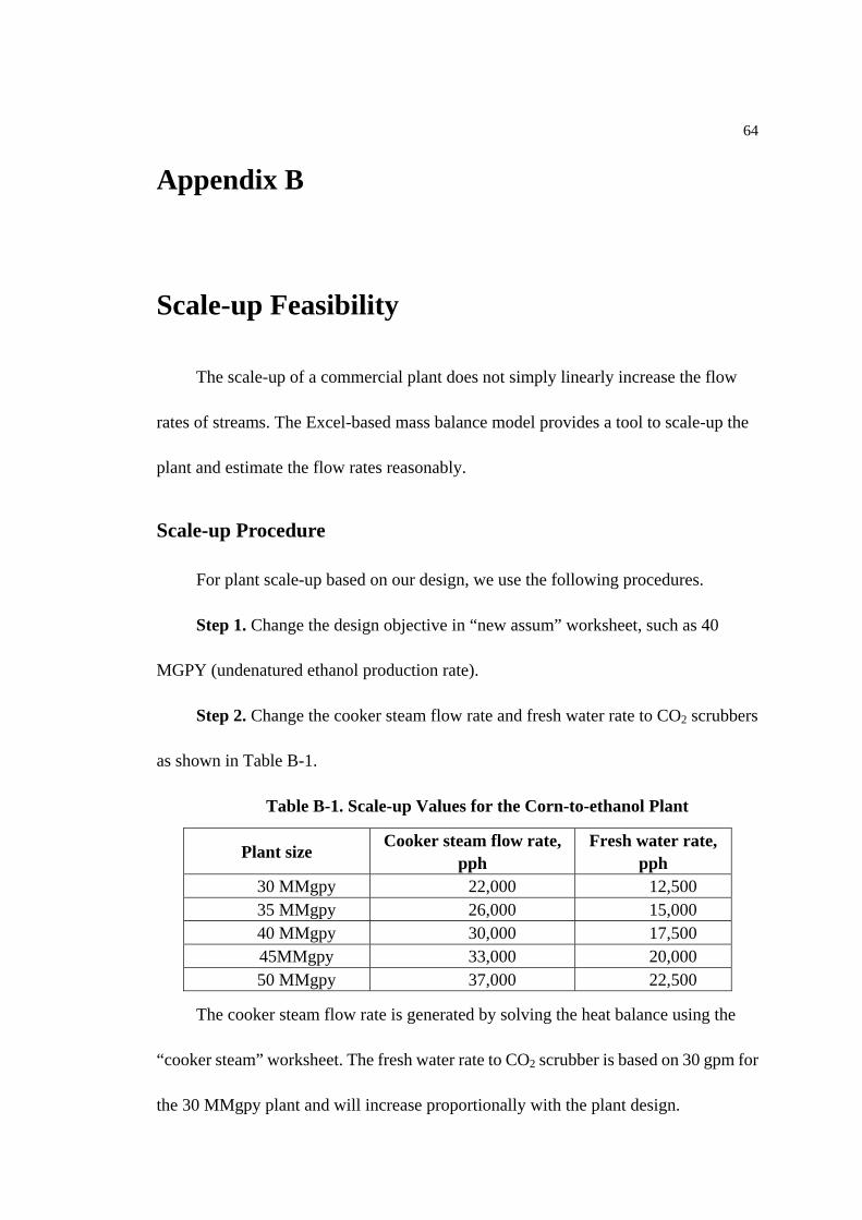
64

Appendix B

Scale-up Feasibility

The scale-up of a commercial plant does not simply linearly increase the flow

rates of streams. The Excel-based mass balance model provides a tool to scale-up the

plant and estimate the flow rates reasonably.

Scale-up Procedure

For plant scale-up based on our design, we use the following procedures.

Step 1. Change the design objective in “new assum” worksheet, such as 40

MGPY (undenatured ethanol production rate).

Step 2. Change the cooker steam flow rate and fresh water rate to CO2 scrubbers

as shown in Table B-1.

Table B-1. Scale-up Values for the Corn-to-ethanol Plant

Plant size Cooker steam flow rate, pph

Fresh water rate, pph

30 MMgpy 22,000 12,500 35 MMgpy 26,000 15,000 40 MMgpy 30,000 17,500 45MMgpy 33,000 20,000 50 MMgpy 37,000 22,500

The cooker steam flow rate is generated by solving the heat balance using the

“cooker steam” worksheet. The fresh water rate to CO2 scrubber is based on 30 gpm for

the 30 MMgpy plant and will increase proportionally with the plant design.

65

Step 3. Check the flow rate in “modified compositions” worksheet.

Energy Consumption Results

Based on our design, following this descrived scale-up procedure, we have

estimated mass balances for different plant sizes. Then, using our design mass balance

results, we have estimated energy consumptions using Aspen Hysys simulations and

enumerated the results in Table B-2. Based on this design, when scaling up from 30

MMgpy to 50 MMgpy, energy consumptions in distillation and evaporation section are

proportionally increased. However, for the DDGS dryer, the energy consumption per

gallon of ethanol produced decreased due to the energy efficiency in a larger dryer. [4]

The energy cost of a rotary dryer (usually used in larger plant) is 65% of that using fired

dryer (usually used in small plants). [27] This estimation shows, for large-scale plants,

the energy consumption should decrease.

Table B-2. Energy Consumption in Plants, MMBtu/hr[7, 19]

Plant size, MMgpy 30 35 40 45 50 Mashing 2.4 2.7 3.1 3.6 3.9 Cooking 31.7 37.0 42.2 47.4 52.6

SSF Neg. Neg. Neg. Neg. Neg. Distillation/Dehydration 53.5 62.1 70.8 79.7 87.9

DDGS Dryer 49.6 55.1 52.9 52.1 53.7 Evaporation 20.4 24.2 27.6 31.1 34.6

Subtotal 157.5 183.9 209.8 236.2 261.8 Electricity demand, kWh 1.02 0.97 0.92 0.88 0.83

Ethanol conversion process, Btu/gal 46,114 45,296 43,049 41,573 40,643Energy Cost, US $/ gallon ethanol 0.195 0.191 0.181 0.174 0.170

Note that the total energy of the corn-to-ethanol conversion process includes the

electricity demand. The electricity demand decreased with the increase of plant size.

66

The electricity demand is1.02 kWh/ gal for undenatured ethanol at 30 MMgpy. In this

study, the electricity demand scale-up uses the formula as below:

Electricity demand = 1.02 * 0.95(new plant size – 30)/5

Results and Discussion

There are the strengths and weaknesses of scale-up using the ExcelTM-based mass

and energy balances spreadsheet.

The disadvantage of this spreadsheet scale-up is that the scale-up result did not

give an exact value for manufacturing cost estimation. Because the spreadsheet used

the same process variables for different plant sizes as a 30 MMpgy plant and estimated

the energy demand for a DDGS dryer by multiplying an efficient parameter.

But this spreadsheet provided an easy-to-use tool for a user to scale-up a plant.

For a new project manager, the spreadsheet can provide a rough data in a reasonable

range and makes a project access a reliable start. For the industrial engineer with

specific process parameters, the spreadsheet can achieve specific information for a

larger plant. The spreadsheet also gives a possibility for a user to calculate the plant

operating limitation and optimize water and energy recycling. Moreover, the

spreadsheet can be combined with economic data, and provide detailed information for

economic analysis.

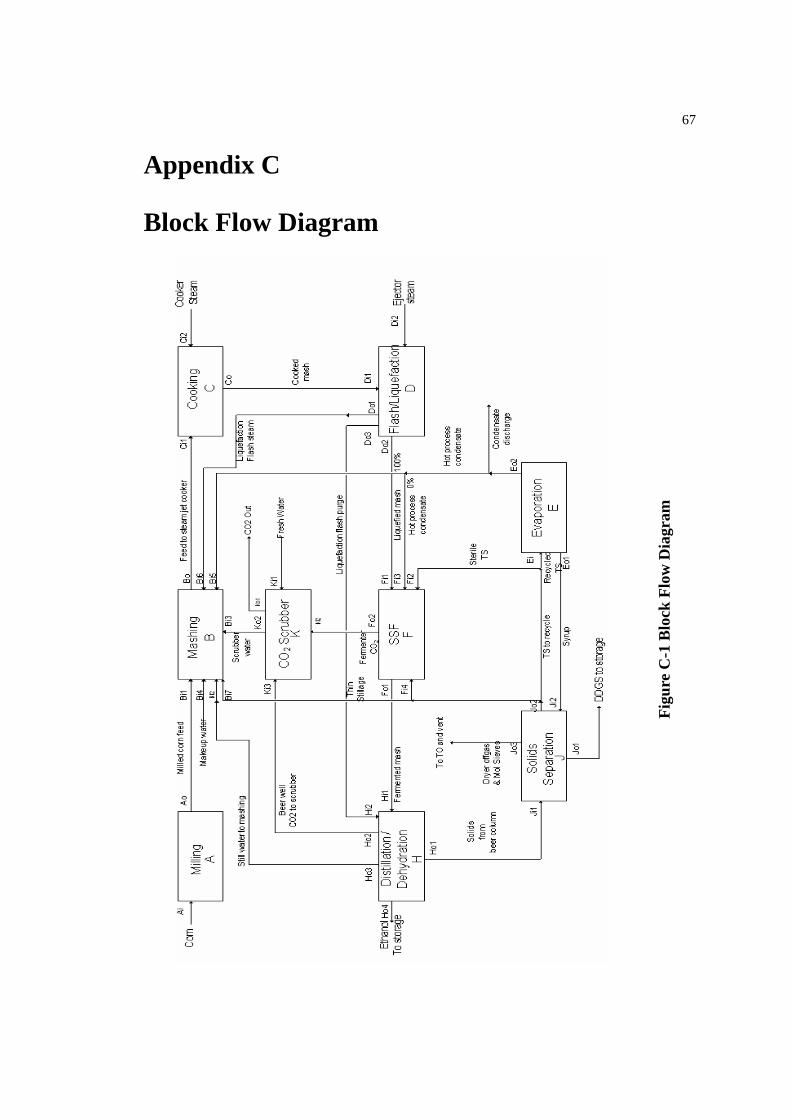
67

Appendix C

Block Flow Diagram

Figu

re C

-1 B

lock

Flo

w D

iagr

am

68

Figu

re C

-2 P

roce

ss

Flow

Dia

gram

69

Appendix D

Excel-based Material Balance Template Guide

The material balance is set up based on the BFD (Block Flow Diagram) shown as

Figure 1 (also saved as the Microsoft Visio file “Block Flow Diagram.vsd”). The material

balance for the plant is saved as “massbalance-05-16-30mgy.xls”. This template file

includes 4 worksheets: “new assum”, “modified composition”, “cooker steam”, and

“water”. The “new assum” worksheet lists design assumptions and allows them to be

modified. The “modified composition” presents the mass balance results for each stream

in the BFD (Block Flow Diagram). The “cooker steam” worksheet contains a simple

calculation for the amount of cooking steam needed to attain the design cooking

temperature of 273°F. The “water” worksheet summarizes the water recycle strategy for

the plant.

General Description 1. In the “new assum” worksheet, variable values with a green background

can be changed to see their effect on the mass balance. Those variables

affect three general design variations. One variation is the production rate

of the plant, e.g. 30 MMgpy. The second variation is the feed corn

composition contents. We specified the composition from the 30 Mmgpy

70 USDA Aspen Plus Model (2000) as a typical example. The third variation

is literature-based assumptions with the initial values typical for a 30

MMgpy plant.

2. Flow compositions entering and leaving the “Flash/Liquefaction” and

“SSF” blocks change because of the reactions in those blocks. Reaction

stoichiometric equations are specified based on the USDA Aspen Model.

3. Some streams’ mass fractions are based on equilibrium data from the

USDA Aspen Model and checked by a Aspen Hysys simulation. Those

streams include the fermenter CO2 stream to CO2 scrubber (Fo2), the beer

well CO2 stream to CO2 scrubber (Ho2), the vented CO2 stream from CO2

scrubber (Ko1), the liquefaction flash purge stream (Hi2), and the

liquefaction flash steam back to mashing (Do1). Ethanol mass fractions in

streams are specified for the thin stillage stream back to mashing section

(Bi7), the stream from the bottom of beer column (Ho1), the beer column

overhead stream (using to determine the thin stillage recycling water), and

the undenatured ethanol stream (Ho4).

4. Note: Variables with the green background can be changed based on the

user’s plant design. Whenever users respecify values with green

background, the template will recalculate the material balance

automatically. But variables influenced by stoichiometry or equilibrium, as

in 2 and 3 above, must be changed by modifying the stoichiometry or

equilibrium equation. For example, if a user wants to increase the ethanol

71 conversion rate from 2.7 gal/bu to 2.8 gal/bu, the material balance can’t

automatically get a 2.8 gal/bu ethanol yield. It is necessary to change the

reaction stoichiometric equations or to change the corn feed composition in

“modified composition”.

Scale-up Procedures by Steps For plant scale-up based on our design, we provide the following procedures.

Step 1. Change the design objective in “new assum” worksheet, such as 40

MGPY (undenatured ethanol production rate).

Step 2. Change the cooker steam flow rate and fresh water rate to CO2 scrubbers

as shown in Table B-1. The cooker steam flow rate is generated by solving heat balance

in “cooker steam” worksheet. The fresh water rate to CO2 scrubber is based on 30gpm for

the 30 MMgpy plant and proportional increasing with the plant design.

Step 3. Check the flow rate in “modified compositions” worksheet.

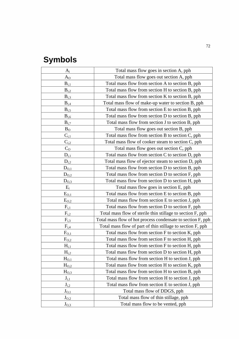
72

Symbols Ai Total mass flow goes in section A, pph AO Total mass flow goes out section A, pph Bi,1 Total mass flow from section A to section B, pph Bi,2 Total mass flow from section H to section B, pph Bi,3 Total mass flow from section K to section B, pph Bi,4 Total mass flow of make-up water to section B, pph Bi,5 Total mass flow from section E to section B, pph Bi,6 Total mass flow from section D to section B, pph Bi,7 Total mass flow from section J to section B, pph BO Total mass flow goes out section B, pph Ci,1 Total mass flow from section B to section C, pph Ci,2 Total mass flow of cooker steam to section C, pph CO Total mass flow goes out section C, pph Di,1 Total mass flow from section C to section D, pph Di,2 Total mass flow of ejector steam to section D, pph DO,1 Total mass flow from section D to section B, pph DO,2 Total mass flow from section D to section F, pph DO,3 Total mass flow from section D to section H, pph Ei Total mass flow goes in section E, pph

EO,1 Total mass flow from section E to section B, pph EO,2 Total mass flow from section E to section J, pph Fi,1 Total mass flow from section D to section F, pph Fi,2 Total mass flow of sterile thin stillage to section F, pph Fi,3 Total mass flow of hot process condensate to section F, pphFi,4 Total mass flow of part of thin stillage to section F, pph FO,1 Total mass flow from section F to section K, pph FO,2 Total mass flow from section F to section H, pph Hi,1 Total mass flow from section F to section H, pph Hi,2 Total mass flow from section D to section H, pph HO,1 Total mass flow from section H to section J, pph HO,2 Total mass flow from section H to section K, pph HO,3 Total mass flow from section H to section B, pph Ji,1 Total mass flow from section H to section J, pph Ji,2 Total mass flow from section E to section J, pph JO,1 Total mass flow of DDGS, pph JO,2 Total mass flow of thin stillage, pph JO,3 Total mass flow to be vented, pph

73

References

[1] Aspen Plus, Release 12.1, Aspen Technology, Inc., Cambridge, MA, 2000 [2] Aspen Physical Property System 12.1 Physical Property Methods and Models,

June, 2003.

[3] Aspen Plus User Guide, 2003, Aspen Technology, Inc.

[4] Barr-Rosin Powder Technology Division, 2005. Rotary Dryers, Coolers and Calciners.

[5] Beck, R. W., Inc. 2005, Renewable Energy Bulletin: Corn to Ethanol

Production Process & Operations and Maintenance Costs.

[6] Broin Company. Press release, Bulletin of Ethanol , November 4, 2004

[7] California energy Commission, 1999. Report to the Governor: Evaluation of Biomass-to-Ethanol Fuel Potential in California

[8] Carlson, Eric C., 1996. Don’t Gamble With Physical Properties For

Simulations, Chemical Engineering Progress, October.

[9] Corn Refiners Association, Inc., Critical Data Tables, (CRA), Washington D. C., 3rd Edition. 2003

[10] Chambers, R.S., Herendeen, R. A., Joyce, J. J. and Penner, P. S., 1979.

Gasohol: Does It or Doesn’t It Produce Positive Net Energy?, Science, VOl. 206, 790-795.

[11] David Andress & Associates, Inc., 2002. Ethanol Energy Balance, November.

[12] Dien, Bruce S.; Bothast, Rodney D.; Nichols, Nancy N.; and Cotts, Michael

A. 2002. Int Sugar Jnl, 1241, (104)

[13] East Kansas Agri-Energy and BBI International , 2001. Ethanol Plant Feasibility Study.

[14] Felder, Richard M. and Rousseau, Ronald W., 1986. Chapter14 Fermentation

of Grain to produce Ethyl Alcohol, Elementary Principles of Chemical

74 Processes, 2nd Edition, John Wiley & Sons.

[15] Fuel Ethanol: A Technological Evolution, Novozymes & BBI International,

June, 2004. [16] Graboski, Michael S. 2002. Fossil Energy Use in the Manufacture of Corn

Ethanol, August, National Corn Growers Association.

[17] Groce, Larry; Bratney Copanies. 2004. Personal correspondence with Prof. Marti Evans, September 24.

[18] Hwang, C. H.; Heldman D. R.; Chao R. R.; and Taylor T. A. 1999. Changes

in specific heat of corn starch due to gelatinization, Journal of food science, vol. 64, No. 1.

[19] The Iowa Department of Agriculture and Land Stewardship Office of

Renewable Fuels, 2001. The Effect of Expanding Ethanol Markets On Ethanol Production, Feed Markets, And the Iowa Economy.

[20] Jacques, K. A.; Lyons, T. P.; and Kelsall, D. R. 2003. The Alcohol Textbook,

4th Edition, Nottingham University Press, Bath, England.

[21] Lemuz, Carlos; Dien, Bruce; Tumbleson, Mike; et al. 2004. Ethanol Yield Determination for Dry Grind Corn Processing, Corn Utilization Conference Proceedings, June 9, (accepted)

[22] Lehninger, Albert L.; Nelson, David L.1993. Principles of Biochemistry,

Worth Publishers, 2nd ed., New York.

[23] McAloon, Andrew; Taylor, Frank; and Yee, Winnie; 2000. Determining the cost of producing ethanol from corn starch and lignocellulosic feedstocks, National Renewable Energy Laboratory/TP-580-28893, October.

[24] Melander, Mark; Bratney Companies; Personal conversation with Prof. Marti

Evans.

[25] Morey, Vance, 2005. Renewable Energy Research, Biosystems and Agricultural Engineering, University of Minnesota.

[26] National Corn Growers Association. The World of Corn 2004.

75 [27] Palmer, Greg, Howes, Tony, 2004. Design and Efficiency Aspenct of Rotary

Dryers, Department of Chemical Engineering, University of Queensland.

[28] Patzek, Tad W. 2004. Thermodynamics of the Corn-Ethanol Biofuel Cycle, CRPS, 23 (6).

[29] Patzek, Tad W. el., 2003. Ethanol from Corn: Clean renewable fuel for the

future, or drain on out resources and pockets, ENVI165-03N, June

[30] Personal discussion with Prof. Terry Tolliver, Washington University in St. Louis

[31] Personal communication with Tom Schroeder by Prof. Heider, Ventiflex

Company. [32] Personal communication with Prof. Robert Heider, Washington University in

St. Louis

[33] Pieper, H.J., Ponitz, H., Zur Gewinnung von Garungsalkohol sus siliertem kornermais, 1973. Chem. Microbiol. Technol. Lebensm. 2, 174-179.

[34] Pimentel, David, 1998. Energy and doller costs of ethanol production with

corn, M. King Hubbert center Newsletter #98/2 [35] Roehr, M., Editor. 2001. The Biotechnology of Ethanol: Classical and Future

Applications. WILEY-VCH, Weinheim, Federal Republic of Germany.

[36] Shapouri, Hosein; Duffield, James A.; and Wang, Michael. 2002. The Energy Balance of Corn Ethanol: An Update, U.S. Department of Agriculture, July.

[37] Shapouri, Hosein, Gallagher, Paul, and Graboski, Michael S., 2002. USDA’s

Plant Survey, USDA

[38] Shapouti, Hosein; Duffield, James; McAloon, Andrew; and Wang Michael, 2004. The 2001 Net Energy Balance of Corn-Ethanol, USDA, OCE http://www.ethanolrfa.org/net_energy_balance_2004.pdf

[39] Sinnott, R. K. 1993. Chemical Engineering Design, Coulson & Richardson’s

Chemical Engineering, Vol. 6, 2nd Edition.

76 [40] Taylor, Frank; Kurantz, Michael, Goldberg, Neil; and Craig, James C., Jr.

1998. Biotechnology Letters 20 (1). [41] Taylor, Frank. 2000. the USDA Aspen Plus model, 30 MMgpy.

[42] Turton, Richard, Richard C. Bailie, Wallace B. Whiting, and Joseph A.

Shaeiwitz, 1998. Analysis, Synthesis, and Design of Chemical Processes, Prentice Hall, Inc.

[43] United State Patent. ASTM Standard E 1344

[44] Vijay Singh, Kent D. Rausch, el. 2001. Modified Dry Grind Ethanol Process,

Publication of the Agricultural Engineering Department UILU No. 7021

[45] Wallace, Robert, Kelly Ibsen, Andrew McAloon, Winnie Yee, 2005. Feasibility Study for Co-Locating and Integrating Ethanol Production Plants fro Corn Starch and Lignocellulosic Feedstocks, National Renewable Energy Laboratory, NREL/TP-510-37092

[46] Wang, M., C. Saricks, D. Santini. 1999. Effects of Fuel Ethanol Use on

Fuel-Cycle Energy and Greenhouse Gas Emissions. U. S. Department of Energy, Argonne National Laboratory, Center for Transportation Research, Argonne, IL.

[47] Rausch, Kent D. 2002. Membrane Technology in the Starch Processing

Industry. Starch, 54: 273-284.

[48] Keeney, D. R., and T. H. Deluca. 1992. Biomass as an Energy Source for the Midwestern U. S., American Journal of Alternative Agriculture, Vol. 7, 137-143

[49] Lorenz, D., and David Morris. 1995. How Much Energy Does it Take to

Make a Gallon of Ethanol? Revised and Updated. Institute for Local Self-Reliance, Washing, DC.

77

Vita

Name: MEI Fan

Birth Date: June 27, 1977

Birth place: Tianshui, P. R. China

Honors:

1. Department Fellowship, Washington University in St. Louis, 2003- present 2. Excellent Student Fellowship, Tsinghua University, China, 2000-2002, 3. Privilege to enter Graduate School of Tsinghua University (with the honor of

being a waiver of admission tests) 4. Outstanding Student Scholarship, 1996-1999 5. Privilege to enter Undergraduate School of Tsinghua University (with the

honor of being a waiver of admission tests) (Only one student can be a waiver of admission tests among 200,000 students in China in1996)

6. First Prize in Provincial High School Chemistry Competition, 1996 7. Third Prize in Provincial High School Physical Competition, 1996

Publications:

a. Fan Mei, M. Evans, C. N. Carpenter, M. Dudukovic, Improving Profitability in the Corn-to-ethanol Plant using Simulation technology, accepted by AIChE 2005 Annual Meeting

b. Changfeng Li, Fan Mei, et.al., Influence of Chain extensibility and Relaxation Spectrum on polymer Induced Drag reduction in Channel flow: A Computational Study, presented at the AIChE 2004 Annual Meeting

c. Fan Mei, Wei Qin and Youyuan Dai, Extraction Equilibriums of Benzoic Acid with Tri-butyl Phosphate in Kerosene and 1-Octanol, J. Chem. Eng. Data, 47(4): 941-943, 2002

d. Shan Jing, Fan Mei, et.al., Fluidization of fine particles in conical beds, Powder Technology 118, 2001:271-274

e. Fan Mei, Wei Qin and Youyuan Dai, Extraction Equilibriums Characteristics of Benzoic Acid, J. Applied Chemistry, 42(5), 2002

May 2006

Short Title: Corn-to-Ethanol Plant Balance Mei, M. S. 2006